Hi-Stat
Discussion Paper Series
No.46
Effects of Human Capital on Farm and Non-Farm Productivity and Occupational Stratification in Rural Pakistan
Takashi Kurosaki and Humayun Khan
November 2004
Hitotsubashi University Research Unit for Statistical Analysis in Social Sciences
A 21st-Century COE Program
Institute of Economic Research
Hitotsubashi University Kunitachi, Tokyo, 186-8603 Japan
http://hi-stat.ier.hit-u.ac.jp/
Effects of Human Capital on Farm and NonFarm Productivityand Occupational Stratification in Rural Pakistan∗
Takashi Kurosaki † and Humayun Khan ‡
November 2004
Abstract
This paper investigates the effects of human capital on productivity using micro panel data of rural households in the NorthWest Frontier Province, Pakistan, where a substantial job stratification is observed in terms of income and education. To clarify the mechanism underlying this stratification, the human capital effects are estimated for wages (individual level) and for selfemployed activities (household level), and for farm and nonfarm sectors. Estimation results show a clear contrast between farm and nonfarm sectors — wages and productivity in nonfarm activities rise with education at an increasing rate, whereas those in agriculture respond only to the primary education.
Keywords: human capital, returns to education, nonfarm employment, selfemployment.
JEL classification codes: O12, J24, Q12.
∗The authors are grateful Christopher Udry, T. N. Srinivasan, T. Paul Schultz, Martin Ravallion, Peter Lanjouw, Xavier Gine, Mir Kalan Shah, Anwar Hussain, Yasu Sawada, Nobu Fuwa, Kei Otsuka, and Katsuhide Isa for valuable comments. We acknowledge financial support from the Ministry of Foreign Affairs, Japan, and SeimeiKai. The views reflected in this paper, however, are solely ours. This paper is a revised version of previous ones titled “Effects of Human Capital on Farm and NonFarm Productivity in Rural Pakistan” (April 2003, February 2004).
†Corresponding author. The Institute of Economic Research, Hitotsubashi University, 21 Naka, Kunitachi, Tokyo 1868603 Japan. Phone: 81425808363; Fax.: 81425808333. Email: [email protected]u.ac.jp.
‡The Institute of Development Studies, NWFP Agricultural University, Peshawar, Pakistan. Email: humayun [email protected].
1 Introduction
In rural areas in contemporary developing countries, nonfarm activities are becoming more
important in determining the welfare of households (Lanjouw and Lanjouw, 2001). As a
result, we often observe job stratification with a substantial income disparity between those
who were successful in finding nonfarm, lucrative jobs and those who were not. Underlying
this stratification is a response of rural households in labor allocation to new economic op
portunities, considering returns to human capital, which may differ from activity to activity.
When farmers decide on their children’s schooling, they are usually motivated by the desire
of finding nonfarm, lucrative jobs for their children. Therefore, investment in human capital
in rural areas is more closely related with nonfarm activities (Huffman, 1980; Yang, 1997;
Fafchamps and Quisumbing, 1999; Lanjouw, 1999; Lanjouw and Lanjouw, 2001; Yang and
An, 2002).
This paper is an empirical attempt to quantify the difference of returns to human
capital across rural activities. Namely, the effects of human capital on farm and nonfarm
productivity are investigated for different educational stages and for different economic activ
ities, using micro panel data of rural households in Pakistan’s NorthWest Frontier Province
(NWFP). The case of NWFP is particularly interesting because the weakness of economic
development in South Asia is concentrated in this region — the incidence of income poverty
is high and the deprivation in human development indicators is more serious than indicated
by income growth. Another reason for studying NWFP economy is the general paucity of
rigorous economic research on Pashtun society, which spreads over NWFP and Afghanistan.
The major contribution of this paper to the human capital literature in development
economics is that a clear contrast between sectors and between employment statuses is shown
through its comprehensive coverage of rural activities after controlling for endogenous selec
tion. This study is one of the few studies that apply the methodology of selection correction
for polychotomous choice models to datasets from developing countries.1 The rural economic
activities are broadly classified into four: nonagricultural wage/salary employment, agricul
tural wage employment, nonagricultural selfemployment, and agricultural selfemployment.
The empirical model is close to that of Yang (1997), who estimated nonlinear production
functions for farm valueadded and linear wage functions for nonfarm wage earnings. Unlike
Yang (1997), however, this paper attempts to include nonfarm enterprises and agricultural
1See Glewwe and Jacoby (1994) for such an example applied to schooling decisions in developing countries.
1
wages and to incorporate nonlinear impacts corresponding to educational stages.
To investigate the difference according to economic sectors, i.e., agriculture vs. non
agriculture, comparable models of returns to human capital are estimated for all sectors that
are relevant for rural households when they allocate labor force. In the recent literature,
Jolliffe (2002) estimated the effects of several alternative measures of household education
on household income, differentiated into farm and nonfarm income. This paper adopts more
detailed decomposition of household income sources than he did.
In characterizing returns to human capital in the rural setting of developing countries,
due attention should be paid to the importance of selfemployment (Newman and Gertler,
1994). Therefore, this paper examines carefully how the education effects on productivity dif
fer according to employment status, i.e., the wage level vs. the productivity of selfemployed
enterprises. Among recent studies, Nielsen and WestergardNielsen (2001) estimated the
effect of education on individual earnings, differentiated into wage and selfemployment in
come sources. This paper is distinguished from their work by allowing returns to labor to
be nonlinear, differentiating returns to labor from returns to assets used in selfemployed
activities, and imputing income from consumption of own farm products properly.
Another contribution of this paper is to give a clue to the controversy regarding the
effects of education on farm productivity. Since Schultz (1961) emphasized the role of educa
tion in improving farm efficiency and in modernizing agriculture, microeconometric studies
to test his hypothesis have been accumulated, showing mixed results from developing coun
tries (Lockheed et al., 1980; Jamison and Lau, 1982; Yang, 1998). In the case of rural
Pakistan, Fafchamps and Quisumbing (1999) found that private returns to education in
farming are insignificant, whereas Kurosaki and Fafchamps (2002) demonstrated that the
effects of schooling years on crop yields per acre are significantly positive. Why have some
studies found positive effects of education on farm productivity while others have not? This
paper gives one possible answer by allowing the effects of education to differ across different
levels of education and at different aggregation levels of farm activities. It is found that the
effect of education is stronger at more aggregate levels, suggesting the importance of human
capital for efficient factor allocation within a farm.
The paper is organized as follows. Section 2 describes the key features of labor allocation
and educational achievement in the study area. Section 3 proposes empirical models to
quantify the effects of education on productivity. Section 4 shows estimation results for the
four broadly classified activities. Section 5 concludes the paper.
2
2 Data and Key Features Identified in the Field
2.1 Data
This paper employs a panel dataset compiled from a sample household survey implemented in
1996 and 1999 in three villages in the Peshawar District of Pakistan’s NWFP. NWFP is one
of the four provinces of Pakistan. Compared with Punjab, which is the center of agriculture
and related industries, and Sind, where the metropolitan city of Karachi is located, NWFP
and Baluchistan could be characterized as economically backward provinces. The incidence
of income poverty (headcount index) in rural NWFP is estimated at 46.5% in 1998/99 (World
Bank, 2002), which is the highest in Pakistan.
Since NWFP is a relatively landscarce province with limited scope for agriculture
led sustained growth, human capital is expected to play a more important role in poverty
eradication. Yet, even in terms of human development, the province is behind the other two
provinces. Literacy rates in NWFP, especially of females, are much lower than in Sind and
Punjab, and NWFP is lagging behind Punjab and Sind in infant mortality rates also. This
disparity, i.e., human development poverty being more serious than income/consumption
poverty, is a notorious characteristic of South Asia as well as Pakistan, to which various
issues of UNDP’s Human Development Reports drew attention. This paper focuses on rural
NWFP because this is a region where this disparity is stark.
Details of the first survey are given by Kurosaki and Hussain (1999) and those of
the second survey are given by Kurosaki and Khan (2001). The reference period for each
survey is fiscal years 1995/96 and 1998/99 respectively. 2 In choosing sample villages in 1996,
we controlled for village size, sociohistorical background, and tenancy structure. At the
same time, to ensure that the cross section data thus generated would provide dynamic
implications, we carefully chose villages with different levels of economic development. The
first criterion was agricultural technology. One of the three sample villages was rainfed,
another semiirrigated, while the other was fullyirrigated. Another criterion was that the
selected villages be located along the ruralurban continuum so that it would be possible
to decipher the subsistence versus market orientation of farming communities in the study
area.
Table 1 summarizes characteristics of the sample villages. Village A is rainfed and
is located some distance from main roads. This village serves as an example of the least
2Pakistan’s fiscal year as well as its agricultural year is the period from July 1 to June 30.
3
developed villages. Village C is fully irrigated and is located close to a national highway,
so serves as an example of the most developed villages. Village B is in between. Sample
households in each village were selected randomly from each type of household classified by
their farm operating status: nonfarm households (with no operated land for cropping)3 and
farm households that include owner, ownercumtenant, and pure tenant farm households.
The distinction among farm households enables us to decipher the effects of land assets on
household welfare.
Out of 355 households surveyed in 1996, 304 were resurveyed in 1999. The most frequent
reason for attrition was migration. Some households have migrated out from the village and
others have sent all their adult males to work in foreign countries or in Pakistani cities.
Among those resurveyed, three had been divided into multiple households, resulting in the
total number of resurveyed households in 1999 as 309.4 In 1999, additional 43 households
were also surveyed as “replacement” samples. This paper, therefore, employs an unbalanced
panel of 398 households, of which 301 are resurveyed households without household division
and 299 are those panel households with complete and comparable information.5
Table 1 also shows characteristics of the panel households. Average household sizes are
larger in Village A than in Villages B and C, reflecting the stronger prevalence of an extended
family system. Average landholding sizes are also larger in Village A than in Villages B and
C. Since the productivity of purely rainfed land is substantially lower than that of irrigated
land, effective landholding sizes are comparable among the three villages. As is shown in
the average household income or consumption per capita, the living standard is the lowest
in Village A and the highest in Village C.6
In the sample villages, yields of wheat (staple food) are not only low on average (the
overall mean was 690 kg/ha in the unirrigated village and 1,760 kg/ha in the irrigated vil
3“Nonfarm” households are defined by the land operation status. Therefore, several households who did not operate any land but worked as farm laborers for wage or kept livestock are classified as “nonfarm” households.
4In the survey, a household is defined as a unit of coresidence and shared consumption. A typical joint family in the region, where married sons live together with the household head who owns their family land along with their wives and children, is treated as one household as long as they share a kitchen. When the household head dies or becomes aged, the land may be distributed among sons, who start to live separately on that occasion. In our survey when we encounter such cases, each family of each son is counted as one household.
5See Appendix 2 for the determinants of attrition. 6During the three years since the first survey, Pakistan’s economy suffered from macroeconomic stagnation
with rising poverty (World Bank, 2002), which hurt the NWFP economy the most severely. Reflecting these macroeconomic shocks, the general living standard declined in the study villages during the period of this study.
4
lages) but also fluctuate widely. The share of wheat consumption met from own production
was less than 30% in the rainfed village (Village A) where wheat yield is the lowest. Even
in Villages B and C where wheat yields are higher, the average percentage was low, in the
range from 20 to 47% (Kurosaki and Hussain, 1999). This situation is attributable to the
low productivity of wheat in Village A and the meager size of land holding in Villages B and
C. In the study area, however, grain markets are well developed, where wheat is available
throughout the year at stable prices thanks to public intervention (Kurosaki, 1996). There
fore, marginal farmers would be better off with higher food security by growing vegetables
on their land and by increasing nonfarm employment, rather than by growing wheat to the
limit on their marginal land.
2.2 Labor Force Allocation and Human Capital
Information on personal details was collected from every household member and every fam
ily member who remitted regularly to the household. The information includes age, sex,
educational background, regular working status, primary occupation, secondary occupation,
average monthly wages/earnings from employment, and so on.
Table 2 shows the distribution of working household members by their employment
status. From those household members whose age is 15 years and above, students, retired
people, and the unemployed are excluded, giving the total number of working members at
1,591 for the total 355 households in 1996 and 1,606 for the total 352 households in 1999.7
Based on each individual’s primary occupation, the table classifies the employment status
into five categories: household work, nonagricultural wage/salary employment, agricultural
wage employment, nonagricultural selfemployment, and agricultural selfemployment.
Agriculture is traditionally the most important source of employment in the study
region. Because there are few large scale farms that are completely dependent on hired
labor, most of those engaged in agriculture are selfemployed. Their labor is sometimes
supplemented by hired labor. Nonagricultural selfemployment activities, or nonfarm en
terprises, are diverse: traditional, castebased services in rural South Asia such as carpenters,
barbers, and blacksmiths (approximately 13% of the individuals selfemployed in nonfarm
enterprises); lowcapital, lowend jobs such as snack hawkers and shoe polishers (15%); and
7Below the age of 15, no female children were reported to have primary occupation, while 37 male children, aged 1014, or 8.4% of that age group, were associated with primary occupation. Among them, 10 worked on their parents’ farm, four on their parents’ nonagricultural enterprises, two on others’ farms, and 21 were employed in nonagricultural wage jobs, mostly in lowpaid sectors.
5
those that require relatively large initial capital such as arms trading, general shops, wheat
mills, and nursery shops (57%). Transportation service is also common (15%), which cov
ers all three types listed above. Nonagricultural wage/salary employment are also diverse,
including daily construction work, wage employment in those listed as nonagricultural self
employment activities, and office/shop work in the nearby towns. Since the size of estab
lishments is universally small for those employees, we may classify them according to their
contract duration — approximately 55% of the nonfarm employees were hired casually on
daily basis, while the rest were hired regularly.
Among males, employment in nonagriculture and selfemployment in agriculture are
more frequently found than the other two. The concentration of female workers on the
category “household work” reflects the effects of purdah, the custom of social seclusion of
women in South Asia. The custom is maintained more strictly in rural NWFP where Pashtun
codes of maintaining family honor reinforce it (Ahmed, 1980). Because of the prevalence of
purdah, male household heads in the study area prefer female family members not to work
outside; when the female members work domestically in productive activities, the heads do
not recognize their work as economically productive unless they are engaged in the marketing
stage also, which is very rare. As a result, the number of female household members who
are engaged in “household work” is abnormally high in Table 2.8 Because of this distortion,
we focus only on male labor allocation and the effects of human capital on it in the following
analysis.
Panel B of Table 2 shows the level and composition of household income corresponding
to the labor allocation in Panel A. The average household income excluding transfers and
remittances is approximately Rs. 70,500, or US$ 1,800, for the average household size of
9.4 members in 1996. The corresponding figure for 1999 is approximately Rs. 61,800, or
US$ 1,300. Consumption declined less than income did, indicating that households have
ex post measures to cope with income risk (Kurosaki, forthcoming). The majority of the
sample households are estimated to lie close to or below the poverty line (Kurosaki and
Hussain, 1999; Kurosaki and Khan, 2001). The composition shares show that the earning
from nonagricultural employment is the most important one, followed by selfemployment
in agriculture and selfemployment in nonagriculture. Therefore, the average income per
There were 15 cases of females employed by others for nonfarm work. Among them, 11 were hired casually (five in construction and six in unspecified works including domestic services) and four were hired regularly (three in lowpaid jobs and one with monthly, moderate salary).
6
8
10
worker in nonfarm selfemployment is highest, followed by that in wage employment in non
agriculture. The average income per worker in agriculture, whether it is selfemployment or
a wage job, is much lower than those in nonagriculture, suggesting a job stratification with
a substantial income disparity. Then what determines the job stratification among these
four activities?
This paper attributes the answer to a difference in returns to human capital in rural
economic activities. Information on age and educational achievement is shown in Table 3,
for the same working males described in Table 2. The average age was 36.0 in 1996 and
34.6 in 1999. The educational achievement is shown in two different forms. Schooling years
correspond to a standard variable in Mincerian models of economic returns to education.9 To
capture nonlinear effects of education associated with educational stages, a series of dummy
variables are also compiled, with no education as a reference group. Among these dummy
variables, the average of the literacy dummies that correspond to primary school education
or above is reported in Table 3. These numbers show that educational achievement of sample
households is indeed low — the average schooling was 3.7 years in 1996 and 4.0 years in 1999;
literacy rate was 43% in 1996 and 48% in 1999.10
The relationship between employment status and human capital variables is also sum
marized in Table 3. The selfemployed are older than employees and those working in agri
culture are older than those in nonagriculture. The difference in educational achievement
is more significant between agricultural vs. nonagricultural jobs than between employment
vs. selfemployment — those engaged in nonagricultural jobs are generally more educated
than those engaged in agricultural jobs.
9To reflect the fact that repetition is common in the study area and skipping is also possible for bright students (Hoodbhoy, 1998; Sawada and Lokshin, 2001), years measured in Pakistan’s standardized education system were used in converting completed grades into completed years of education. Up to the twelfth grade, the system is standardized as follows: primary education of five years beginning from the age of five or six, either by primary or mosque schools; midd le education of three years; secondary education of two years; higher secondary education of two years. After completing the twelfth grade and passing the “intermediate” FA/FSc degree examination, degree classes are taught at universities and colleges with various years of instruction depending on the specialization (Hoodbhoy, 1998).
Achievement in female education is much lower than that for males reported here. In 1996, average schooling was 0.5 years and the literacy rate was 7.6% for female counterparts (Kurosaki, 2001). As Sawada and Lokshin (2001) showed, the gender gap in education is more influenced by the gender gap in the initial enrollment into primary education. In our case also, the gender gap in the average schooling years becomes much smaller when only those who completed primary education are compared.
7
3 Empirical Specification
The descriptive analysis above suggests that rural nonagricultural activities are associated
with higher earnings per worker and higher education levels of male workers involved. To
investigate whether or not this association can be explained by a difference in returns to
human capital, this section proposes empirical models that are comparable between the
four rural activities and control for endogenous selection of the activities. Before presenting
empirical specifications, a brief discussion on the theory would help in aligning the issue of
labor allocation with that of returns to human capital.
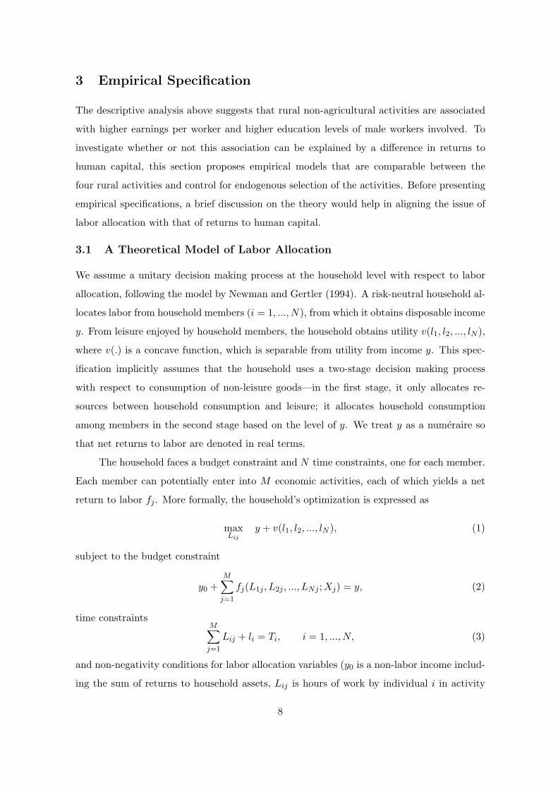
3.1 A Theoretical Model of Labor Allocation
We assume a unitary decision making process at the household level with respect to labor
allocation, following the model by Newman and Gertler (1994). A riskneutral household al
locates labor from household members (i = 1, ..., N), from which it obtains disposable income
y. From leisure enjoyed by household members, the household obtains utility v(l1, l2, ..., lN ),
where v(.) is a concave function, which is separable from utility from income y. This spec
ification implicitly assumes that the household uses a twostage decision making process
with respect to consumption of nonleisure goods—in the first stage, it only allocates re
sources between household consumption and leisure; it allocates household consumption
among members in the second stage based on the level of y. We treat y as a numeraire so
that net returns to labor are denoted in real terms.
The household faces a budget constraint and N time constraints, one for each member.
Each member can potentially enter into M economic activities, each of which yields a net
return to labor fj . More formally, the household’s optimization is expressed as
max Lij
y + v(l1, l2, ..., lN ), (1)
subject to the budget constraint
M� y0 + fj(L1j , L2j , ..., LNj ;Xj) = y, (2)
j=1
time constraints M�
Lij + li = Ti, i = 1, ..., N, (3) j=1
and nonnegativity conditions for labor allocation variables (y0 is a nonlabor income includ
ing the sum of returns to household assets, Lij is hours of work by individual i in activity
8
� �
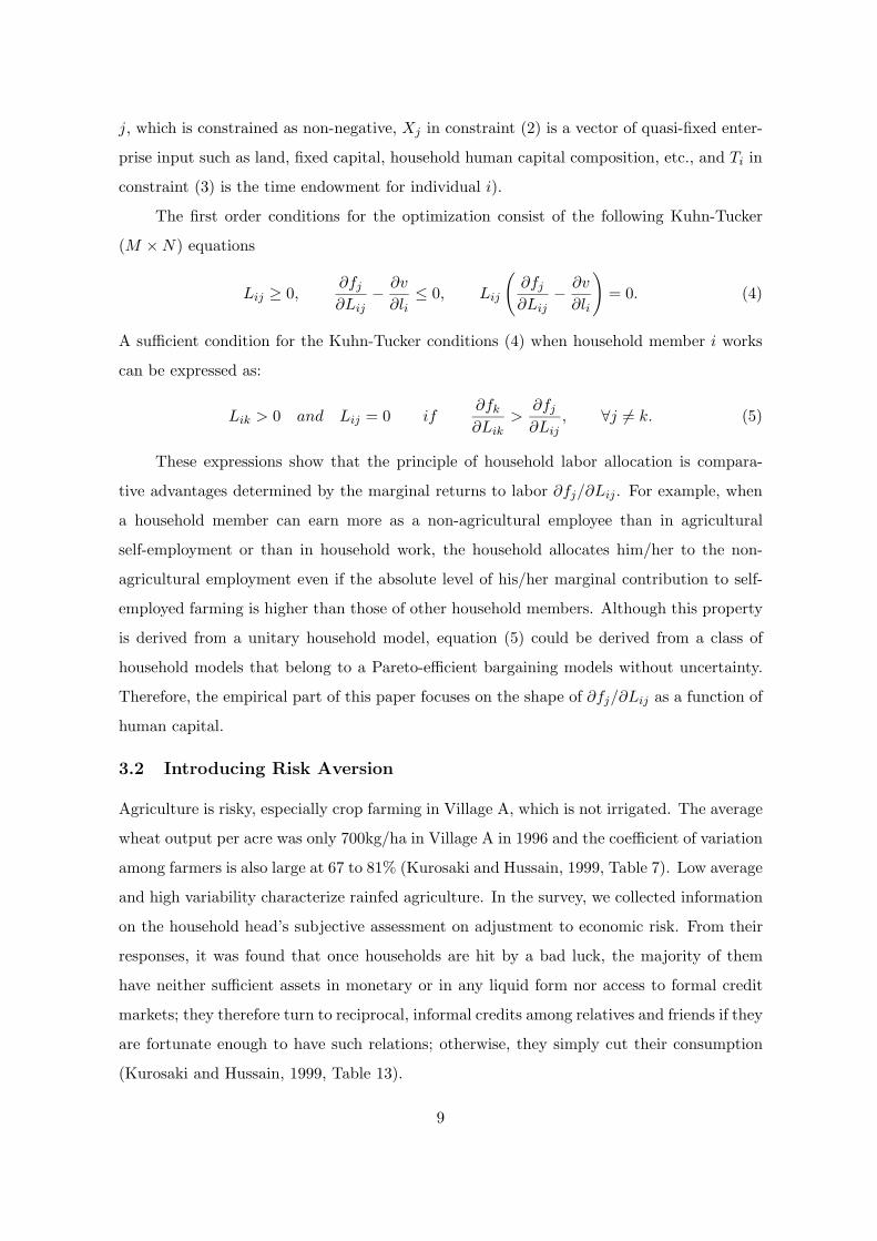
j, which is constrained as nonnegative, Xj in constraint (2) is a vector of quasifixed enter
prise input such as land, fixed capital, household human capital composition, etc., and Ti in
constraint (3) is the time endowment for individual i).
The first order conditions for the optimization consist of the following KuhnTucker
(M × N) equations
Lij ≥ 0, ∂fj ∂v ≤ 0, Lij
∂fj ∂v (4)
∂Lij −
∂li ∂Lij −
∂li = 0.
A sufficient condition for the KuhnTucker conditions (4) when household member i works
can be expressed as:
Lik > 0 and Lij = 0 if ∂fk
> ∂fj
, ∀j = k. (5)∂Lik ∂Lij
�
These expressions show that the principle of household labor allocation is compara
tive advantages determined by the marginal returns to labor ∂fj/∂Lij . For example, when
a household member can earn more as a nonagricultural employee than in agricultural
selfemployment or than in household work, the household allocates him/her to the non
agricultural employment even if the absolute level of his/her marginal contribution to self
employed farming is higher than those of other household members. Although this property
is derived from a unitary household model, equation (5) could be derived from a class of
household models that belong to a Paretoefficient bargaining models without uncertainty.
Therefore, the empirical part of this paper focuses on the shape of ∂fj/∂Lij as a function of
human capital.
3.2 Introducing Risk Aversion
Agriculture is risky, especially crop farming in Village A, which is not irrigated. The average
wheat output per acre was only 700kg/ha in Village A in 1996 and the coefficient of variation
among farmers is also large at 67 to 81% (Kurosaki and Hussain, 1999, Table 7). Low average
and high variability characterize rainfed agriculture. In the survey, we collected information
on the household head’s subjective assessment on adjustment to economic risk. From their
responses, it was found that once households are hit by a bad luck, the majority of them
have neither sufficient assets in monetary or in any liquid form nor access to formal credit
markets; they therefore turn to reciprocal, informal credits among relatives and friends if they
are fortunate enough to have such relations; otherwise, they simply cut their consumption
(Kurosaki and Hussain, 1999, Table 13).
9
� �
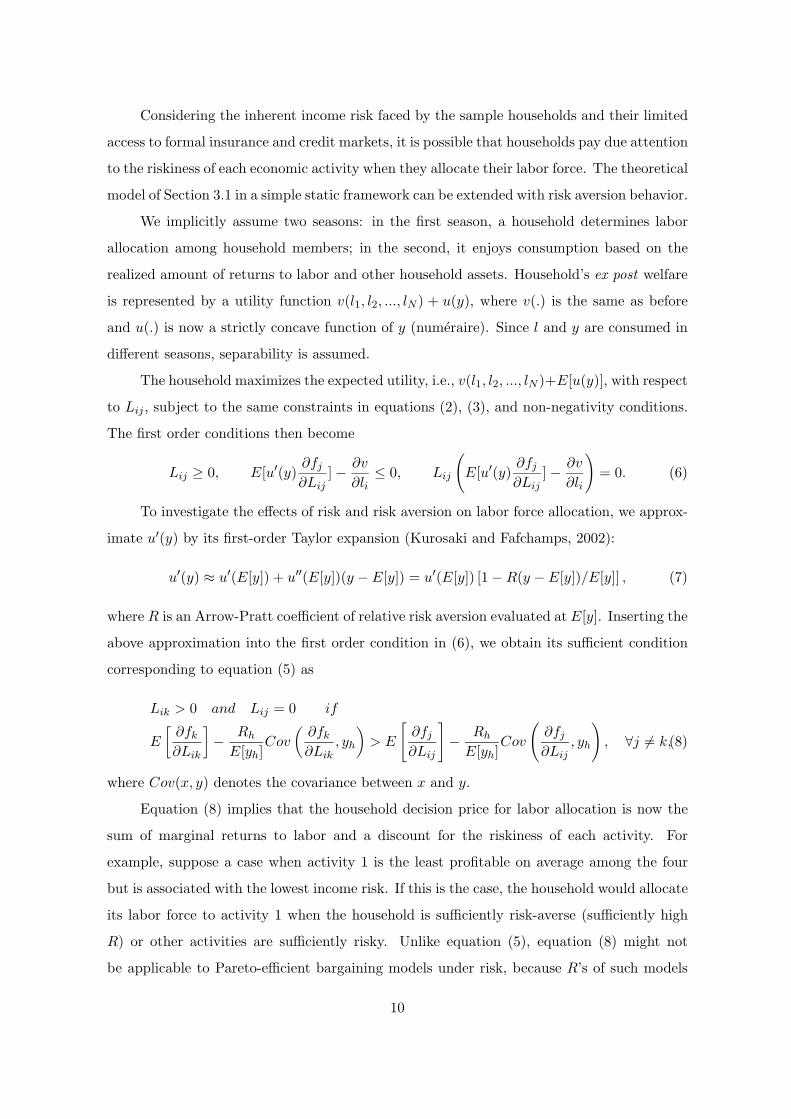
Considering the inherent income risk faced by the sample households and their limited
access to formal insurance and credit markets, it is possible that households pay due attention
to the riskiness of each economic activity when they allocate their labor force. The theoretical
model of Section 3.1 in a simple static framework can be extended with risk aversion behavior.
We implicitly assume two seasons: in the first season, a household determines labor
allocation among household members; in the second, it enjoys consumption based on the
realized amount of returns to labor and other household assets. Household’s ex post welfare
is represented by a utility function v(l1, l2, ..., lN ) + u(y), where v(.) is the same as before
and u(.) is now a strictly concave function of y (numeraire). Since l and y are consumed in
different seasons, separability is assumed.
The household maximizes the expected utility, i.e., v(l1, l2, ..., lN )+E[u(y)], with respect
to Lij , subject to the same constraints in equations (2), (3), and nonnegativity conditions.
The first order conditions then become
∂v ∂v Lij ≥ 0, E[u�(y)
∂fj ]∂Lij
− ∂li
≤ 0, Lij E[u�(y) ∂fj ] (6)∂Lij
− ∂li
= 0.
To investigate the effects of risk and risk aversion on labor force allocation, we approx
imate u�(y) by its firstorder Taylor expansion (Kurosaki and Fafchamps, 2002):
u�(y) ≈ u�(E[y]) + u��(E[y])(y − E[y]) = u�(E[y]) [1 − R(y − E[y])/E[y]] , (7)
where R is an ArrowPratt coefficient of relative risk aversion evaluated at E[y]. Inserting the
above approximation into the first order condition in (6), we obtain its sufficient condition
corresponding to equation (5) as
Lik > 0 and Lij = 0 if � � � � � � � � ∂fk Rh ∂fk ∂fj Rh ∂fj
E ∂Lik
− E[yh]
Cov ∂Lik
, yh > E Cov , yh , ∀j = k,(8)∂Lij
− E[yh] ∂Lij
�
where Cov(x, y) denotes the covariance between x and y.
Equation (8) implies that the household decision price for labor allocation is now the
sum of marginal returns to labor and a discount for the riskiness of each activity. For
example, suppose a case when activity 1 is the least profitable on average among the four
but is associated with the lowest income risk. If this is the case, the household would allocate
its labor force to activity 1 when the household is sufficiently riskaverse (sufficiently high
R) or other activities are sufficiently risky. Unlike equation (5), equation (8) might not
be applicable to Paretoefficient bargaining models under risk, because R’s of such models
10
are likely to vary for each individual, reflecting individual members’ risk preferences and
bargaining rules.
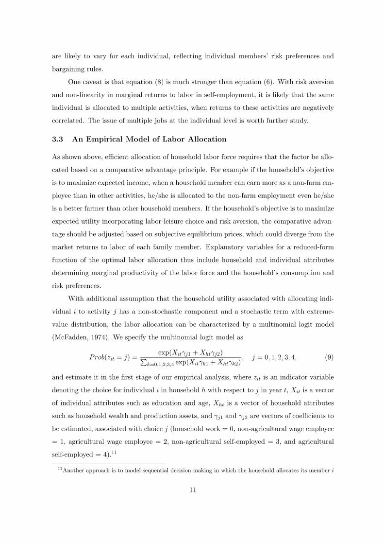
One caveat is that equation (8) is much stronger than equation (6). With risk aversion
and nonlinearity in marginal returns to labor in selfemployment, it is likely that the same
individual is allocated to multiple activities, when returns to these activities are negatively
correlated. The issue of multiple jobs at the individual level is worth further study.
3.3 An Empirical Model of Labor Allocation
As shown above, efficient allocation of household labor force requires that the factor be allo
cated based on a comparative advantage principle. For example if the household’s objective
is to maximize expected income, when a household member can earn more as a nonfarm em
ployee than in other activities, he/she is allocated to the nonfarm employment even he/she
is a better farmer than other household members. If the household’s objective is to maximize
expected utility incorporating laborleisure choice and risk aversion, the comparative advan
tage should be adjusted based on subjective equilibrium prices, which could diverge from the
market returns to labor of each family member. Explanatory variables for a reducedform
function of the optimal labor allocation thus include household and individual attributes
determining marginal productivity of the labor force and the household’s consumption and
risk preferences.
With additional assumption that the household utility associated with allocating indi
vidual i to activity j has a nonstochastic component and a stochastic term with extreme
value distribution, the labor allocation can be characterized by a multinomial logit model
(McFadden, 1974). We specify the multinomial logit model as
exp(Xitγj1 + Xhtγj2)Prob(zit = j) = �
k=0,1,2,3,4 exp(Xitγk1 + Xhtγk2), j = 0, 1, 2, 3, 4, (9)
and estimate it in the first stage of our empirical analysis, where zit is an indicator variable
denoting the choice for individual i in household h with respect to j in year t, Xit is a vector
of individual attributes such as education and age, Xht is a vector of household attributes
such as household wealth and production assets, and γj1 and γj2 are vectors of coefficients to
be estimated, associated with choice j (household work = 0, nonagricultural wage employee
= 1, agricultural wage employee = 2, nonagricultural selfemployed = 3, and agricultural
selfemployed = 4).11
11Another approach is to model sequential decision making in which the household allocates its member i
11

�
The multinomial logit model can be estimated by a maximum likelihood method. Then,
ˆthe fitted probability of individual i working in activity j, Prob(zit = j) is given by expression
(9) with γj1 and γj2 replaced by their estimates ˆ γj2. Similarly, the fitted probability γj1 and ˆ
of household h with its member(s) working in activity j is given by
ˆ �
=j exp(Xit ˆ γk2)k γk1 + Xht ˆProb(zht = j) = 1− ��
k exp(Xit ˆ γk2) . (10)
γk1 + Xht ˆi∈h
These fitted values are used to calculate selection terms in the secondstage estimation ex
plained below.
3.4 Determinants of Wage
Assuming wage labor markets to be exogenous to household decisions, the unit wage becomes
a function of the human capital of the employee, Xit. To capture this idea, a standard Mincer
equation is estimated in which ln Wijt is regressed on Xit, where Wijt is the wage level of
individual i working in activity j (=1, 2), in year t.
Two econometric issues are addressed in this paper. The first is sample selection.
Because Wijt is observed only when individual i works in j = 1 or 2, an error term to
the Mincer equation conditional on this selection has nonzero mean. To control for this,
a twostage procedure is adopted in which a correction term λijt compiled from estimation
results of equation (9) is added as an additional regressor.12 Assuming that the error term
to the wage equation is distributed normally, we adopt the correction term based on the
general transformation of error terms to normality (Lee, 1983), because it facilitates a feasible
computation of a selection term for the householdlevel regression in the next subsection.
λijt ≡ φ[Φ−1[ ˆThe correction term is defined as ˆ
ˆ Prob(zit=j)]] , where φ[.] and Φ[.] are density and
Prob(zit=j)
ˆdistribution functions for a standard normal variable and Prob(zit = j) is obtained from the
firststage multinomial logit model. If at least one variable in Xh in (9) does not affect wages
directly but affects it indirectly through the activity choice, the secondstage wage regression
is identified.
Another econometric issue is unobserved characteristics that affect wages received by
those who work in the wage sector. An example is worker’s ability that is known to the
to the wage sector versus the selfemployment sector in the first stage and then allocates him to agriculture or nonagriculture in the second stage conditional on the choice made in the first stage. The firststage choice can be modeled in a multinomial probit framework as well, in which the axiom of independence of irrelevant alternatives can be relaxed. Relaxing the assumption that the choices are exclusive is also worth exploring, since several individuals have secondary jobs as well (see note 2 of Table 2). Robustness of our results with respect to these approaches is left for a future investigation.
12This procedure enables us to obtain consistent estimates, although they are not fully efficient.
12
household but not observable to the econometrician. To minimize the bias from omitting
these unobservable variables, a household specific effect, αh, is added to the wage regression.
With household panel data, we can control for αh by either fixed or random effect specifi
cation. Since the fixed effect specification may exaggerate measurement error problems, we
adopt the random effect specification as long as Hausman test cannot reject at 1% level the
null hypothesis that Xi and αh are uncorrelated.
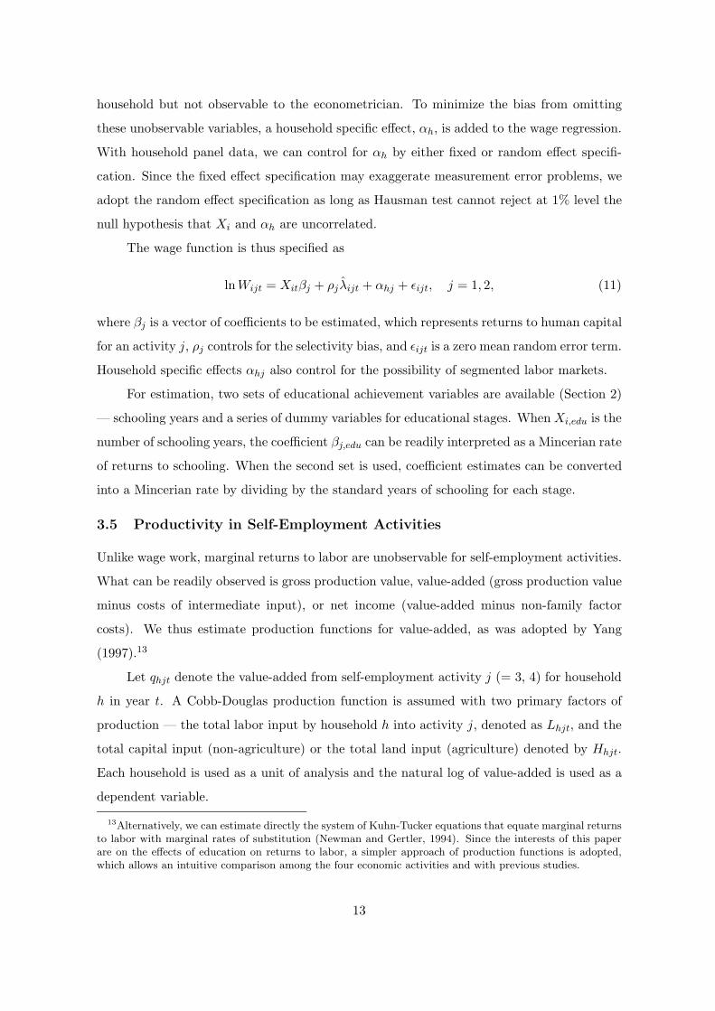
The wage function is thus specified as
ˆln Wijt = Xitβj + ρjλijt + αhj + �ijt, j = 1, 2, (11)
where βj is a vector of coefficients to be estimated, which represents returns to human capital
for an activity j, ρj controls for the selectivity bias, and �ijt is a zero mean random error term.
Household specific effects αhj also control for the possibility of segmented labor markets.
For estimation, two sets of educational achievement variables are available (Section 2)
— schooling years and a series of dummy variables for educational stages. When Xi,edu is the
number of schooling years, the coefficient βj,edu can be readily interpreted as a Mincerian rate
of returns to schooling. When the second set is used, coefficient estimates can be converted
into a Mincerian rate by dividing by the standard years of schooling for each stage.
3.5 Productivity in SelfEmployment Activities
Unlike wage work, marginal returns to labor are unobservable for selfemployment activities.
What can be readily observed is gross production value, valueadded (gross production value
minus costs of intermediate input), or net income (valueadded minus nonfamily factor
costs). We thus estimate production functions for valueadded, as was adopted by Yang
(1997).13
Let qhjt denote the valueadded from selfemployment activity j (= 3, 4) for household
h in year t. A CobbDouglas production function is assumed with two primary factors of
production — the total labor input by household h into activity j, denoted as Lhjt, and the
total capital input (nonagriculture) or the total land input (agriculture) denoted by Hhjt.
Each household is used as a unit of analysis and the natural log of valueadded is used as a
dependent variable.
13Alternatively, we can estimate directly the system of KuhnTucker equations that equate marginal returns to labor with marginal rates of substitution (Newman and Gertler, 1994). Since the interests of this paper are on the effects of education on returns to labor, a simpler approach of production functions is adopted, which allows an intuitive comparison among the four economic activities and with previous studies.
13
Three econometric issues are addressed in this paper. The first is sample selection.
Because qhjt is observed only when household h is involved in j = 3 or 4, an error term to
the valueadded equation conditional on this selection has nonzero mean. To control for this,
Lee’s (1983) general transformation of error terms to normality is adopted, as in the case of
wage functions. Under the assumption of normality of the error terms to the valueadded
λhjt ≡ φ[Φ−1[ ˆ ˆfunctions, the correction term is defined as ˆ Prob(zht =j)]] , where Prob(zht = j) is ˆProb(zht =j)
defined in equation (10).
The second econometric issue is a potential correlation between the error terms to
the dependent variables on the one hand and righthandside variables on the other hand.
The correlation could occur when the righthandside variables are endogenous to household
decisions even in the short run. Another reason for the potential correlation is measurement
errors. These two problems are likely to be serious for factor inputs, especially labor inputs.
To control for these problems, instruments are used for factor inputs and some other right
handside variables.
The third issue is unobserved characteristics that affect the productivity of enterprises.
In farm production, land quality might differ from farm to farm, about which precise infor
mation is lacking in our dataset. In both farm and nonfarm enterprises, households could
be heterogeneous with respect to managerial ability. To minimize the bias from omitting
these unobservable variables, a household specific effect, αh, is added to the valueadded
functions.
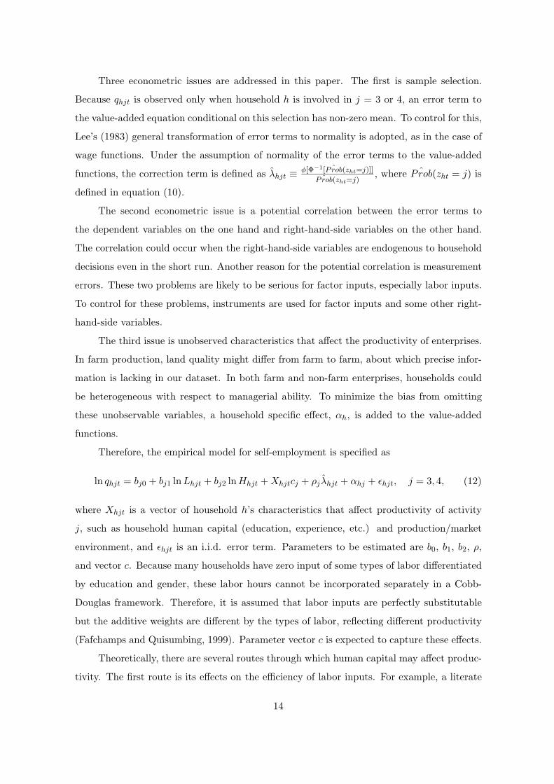
Therefore, the empirical model for selfemployment is specified as
ˆln qhjt = bj0 + bj1 ln Lhjt + bj2 ln Hhjt + Xhjtcj + ρjλhjt + αhj + �hjt, j = 3, 4, (12)
where Xhjt is a vector of household h’s characteristics that affect productivity of activity
j, such as household human capital (education, experience, etc.) and production/market
environment, and �hjt is an i.i.d. error term. Parameters to be estimated are b0, b1, b2, ρ,
and vector c. Because many households have zero input of some types of labor differentiated
by education and gender, these labor hours cannot be incorporated separately in a Cobb
Douglas framework. Therefore, it is assumed that labor inputs are perfectly substitutable
but the additive weights are different by the types of labor, reflecting different productivity
(Fafchamps and Quisumbing, 1999). Parameter vector c is expected to capture these effects.
Theoretically, there are several routes through which human capital may affect produc
tivity. The first route is its effects on the efficiency of labor inputs. For example, a literate
14
laborer will be able to follow the instruction of a labor task more precisely. In other words,
what matters to production is not the amount of hours of labor Lhjt but the amount adjusted
for its quality. Second, the accumulation of human capital might improve overall technical
efficiency in production. Third, the accumulation of human capital might improve allocative
efficiency at the household level. For example, farms with higher human capital might be
able to obtain a higher profit by allocating production factors more efficiently. This could
occur either because a farm manager with higher human capital is more able to allocate
resources in a way closer to what maximizes the expected profit, than a manager with lower
human capital, or, because a farm household with higher human capital would behave in a
less risk averse way thanks to its higher ability to cope with risk, even when both types of
farms are equally able to adopt the expected profit maximizing plan. We can investigate
whether or not the third factor is important by estimating agricultural valueadded functions
at different aggregation levels. If the effects of education on the farmlevel valueadded are
larger than those on valueadded of individual crops, the difference could be attributable to
educated farmers’ superiority in allocating factors across crops.
For estimation, several sets of educational variables are available. Possible choices
include the maximum or minimum of education among all household members, the average
(or median) of all household members, the average (or median) of those household members
who work in the household selfemployment business, the education level of the household
head, and so on (Jolliffe, 2002; Yang, 1998). Because of the small sample size and high
collinearity among these variables, simultaneous inclusion of these variables did not work
well. Therefore, each of these choices was tried in the initial runs and the one that resulted
in the best fit in terms of adjusted R2 is reported below.
4 Estimation Results
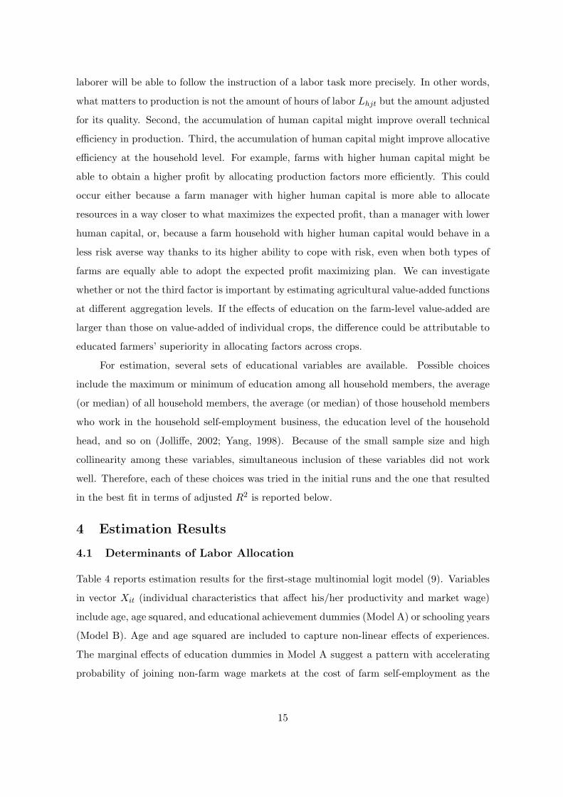
4.1 Determinants of Labor Allocation
Table 4 reports estimation results for the firststage multinomial logit model (9). Variables
in vector Xit (individual characteristics that affect his/her productivity and market wage)
include age, age squared, and educational achievement dummies (Model A) or schooling years
(Model B). Age and age squared are included to capture nonlinear effects of experiences.
The marginal effects of education dummies in Model A suggest a pattern with accelerating
probability of joining nonfarm wage markets at the cost of farm selfemployment as the
15
education level goes up. This is confirmed by negative effects of the squared term of male
schooling years on joining nonfarm wage markets in Model B. Thus the probability of
joining nonfarm wage markets out of selfemployment farming increases with education at
an increasing rate. The effects of age show an inverted U shape for farm and nonfarm wage
employment and an U shape for farm selfemployment.
The marginal effects of Xht show that households with more adult male members and
less dependent members are more likely to send their labor force to outside employment.
Households with land assets are more likely to send their labor force to their own farms.
These results imply that the necessity of family labor on family farms is an important
determinant for the choice whether or not a household sends household members to non
agricultural wage jobs.
4.2 Effects of Human Capital on NonAgricultural Wages
With the sample selection term obtained from the results above, the secondstage wage equa
tion (11) is estimated for nonagricultural wage earners.14 The dependent variable is natural
log of average monthly wage from nonagricultural employment. In estimation, an intercept
dummy for the second survey is added to control for macro shocks. Estimation results are
shown in Table 5, based on a random effect specification. Although χ2 statistics for Hausman
test is somewhat large, it is not larger than the 1% significance level. Therefore, random
effect estimation results are reported, which are likely to be more robust to measurement
errors than fixed effect results.15
Estimation results show that there are significantly positive effects of education on the
wage level. A worker with primary education is expected to be paid 17% (≈ e0.154 − 1) higher
than a nonliterate worker (reference group); with middle school education, 31% higher; and
14Xht in (9) serve as identifying variables for the selection term. We assume that household asset variables that are closely related with farming such as land holding do not directly affect wages paid by others for nonagricultural works but only indirectly through activity choices. Although it is possible that these variables may capture unobservable ability of individuals in implementing nonagricultural work so that they affect nonagricultural wages directly, our field observations suggest that this is unlikely. For example, the nutritionbased efficiency wage theory suggests that individuals from landed family are paid higher due to their superior nutrition conditions. This is unlikely among villagers in the study areas, since little difference was observed in calorie intake across land holding classes.
15The returns to schooling reported in this paper could be an overestimate for rates of return expected from education investment on a random basis, if more able children are selected by the parents or by the community to receive higher education (innate ability bias). The bias may not be large since we utilize panel information to control for householdlevel unobservables by αh. Furthermore, the consensus in the literature is that the upward ability bias may exist but is relatively small (Card, 1999), which is applicable to the case of Pakistan as well (Alderman et al., 1996; 2001).
16
with high and higher school education, 64% higher (Model A). These parameters imply the
following Mincerian rates of returns: 3.1% for education up to the primary level, 3.4% for
education up to the middle level, and 4.4% for education up to the secondary and higher
level; or 3.9% for additional middle education after primary education and 5.8% for additional
higher education after middle education. This range is consistent with the estimates in earlier
studies on the returns to schooling in rural nonfarm activities in Pakistan (Fafchamps and
Quisumbing, 1999; Alderman et al., 1996). When the schooling year and its quadratic term
are included as education variables (Model B), only the positive coefficient on the quadratic
term is statistically significant. These results suggest a possibility that return to education
increases with education at an increasing rate, which is consistent with results for labor
market participation (Table 4).
Since nonfarm wage employment is diverse, distinguishing various types with more
disaggregation, e.g., by industries or by the size of establishments, could be important. Our
samples do not have sufficient variation in the establishment size. Preliminary examination
showed that wages were not different across industries but substantially different whether
a person is hired casually or regularly. Therefore, we extended the model in (9) by distin
guishing these two types of nonagricultral wage employment and reestimated the Mincerian
model in (11) separately for the two types. Since the difference of the coefficients was not
statistically significant except for the intercept, we merged them with an employment type
dummy. Estimation results are reported as Model C in Table 5. In effect, the coefficient
on the dummy in Model C shows the treatment effect of working in regularlyhired activity
with the endogenous selection controlled for. The dummy variable is significantly positive,
indicating that wages for the regularly hired were on average 60% (≈ e0.474 − 1) higher than
those for the casually hired.16 The coefficients on education in Model C are much smaller
than those in Model A. This is because more educated individuals are more likely to work
regularly. Education thus not only increases the wage in nonagriculture but also increases
the probability of working in nonagricultural activities with higher and stable payment.
Among other human capital variables in vector Xi, age as a proxy for job experience
shows an inverted Ushape, with both coefficients on linear and quadratic terms significant.
Wage is maximized at the age range of 42 to 47 years, depending on the model. These
Some of this difference might be due to the difference in the intensity of employment in a month, although we corrected for the difference in working days by using daily earnings multiplied by the standard number of monthly working days for the casuallyhired, not the observed monthly earnings.
17
16
results suggest that productivity in nonagricultural wage work responds positively with
experience but at a diminishing rate. The selection term is significantly positive in all the
models, indicating a positive selection. Individuals whose propensity to be employed in non
agrucluture is high are expected to earn more even after controlling for the direct effects of
their individual attributes on wages.
4.3 Effects of Human Capital on Agricultural Wages
Table 6 reports estimation results for agricultural wage earners. The dependent variable is
natural log of average monthly wages from agricultural employment.
In sharp contrast to results in Table 5, only the coefficient on primary education dummy
is significant with about 3.8% Mincerian returns (Mode A). Education higher than the pri
mary level does not seem to contribute to higher agricultural wages. When both linear
and quadratic terms of schooling years are included (Model B), both are significant with
inverted U shape, implying that marginal returns to education becomes negative at more
than five years of schooling (i.e., standard years of primary schooling in Pakistan). Age
and age squared show an inverted Ushape but the coefficients are smaller than those for
nonagricultural wages.
The nonresponse of farm wages to higher education is understandable considering the
nature of the farm labor market in the study region. Most of these workers are hired for
unskilled, manual work on the farm such as weeding, harvesting, transporting, etc. It is
no wonder that job experiences or education do not contribute much to improvement in
productivity of such works. The selection term is positive but not statistically significant.
4.4 Effects of Human Capital on NonFarm Enterprise Productivity
Production function (12) is estimated for nonagricultural selfemployment. The dependent
variable is natural log of valueadded from nonfarm enterprises. Labor input is measured
by the monetary sum of wages actually paid to hired workers and imputed wages for family
workers using the same wages or village average wages imputed at daily basis. Capital input
is defined as the total capital used in production, approximated by the machinery/equipment
depreciation and land rents for the nonfarm enterprise. Since the two factors of production,
labor and capital, are determined endogenously by the household and they are also likely to
suffer from measurement errors, they are replaced by their fitted values using other right
handside variables, the acreage of agricultural land owned by the household, the number
18
of adult males, the net value of household assets (transportation and durable consumption
goods), and the value of livestock (both levels and logs) as instruments.
Two stage least squares random effect estimation results are reported in Table 7. The
coefficients on both of the production factors are statistically significant. Elasticities of pro
duction with respect to the two production factors are estimated in a reasonable range, with
their sum around 0.83, indicating slightly decreasing returns to scale in nonfarm enterprises
in the study area.
Regarding the effects of education variables, the average education among those house
hold members who are engaged in the nonfarm business performed marginally better than
other specifications in terms of adjusted R2. This could be due to the fact that the number
of those engaged in nonfarm business within a household is not large and they do not always
include the household head and the individual with the highest education. The coefficients on
educational stage dummies show significantly positive effects with higher reward for higher
education (Model A). This is similar to the results for nonfarm wages but the difference
among educational stages is larger. When educational achievement dummies are replaced
by schooling years, their coefficients are insignificant when both linear and quadratic terms
are included but a model with a quadratic term only has a significantly positive coefficient
and fits the data marginally better than a model with a linear term only (not reported).
Coefficients on the age of the household head and its quadratic term show an Ushape, but
only the quadratic term is significant in both models. This seems to suggest that experience
is associated with an increasing return in managing nonfarm enterprises. The coefficient
on the sample selection term is close to zero and not statistically significant, suggesting
that errors in labor allocation decisions and those in valueadded functions are not strongly
correlated.
Since nonfarm enterprises are diverse, distinguishing various types of nonfarm activ
ities with more disaggregation, e.g., lowend type jobs like hawkers and highend type jobs
like wheat mill owners, could be important (Lanjouw, 1999; Lanjouw and Lanjouw, 2001).
Considering the limited number of observations, a dummy variable for those selfemployed
activities that are carried out in a permanent business space (for example, shop space or
workshop space) is included in Model B. Since the dummy variable could be endogenous,
the selection term was reestimated by extending the model in (9) by distinguishing these two
types of nonagricultral selfemployment. The dummy variable has a significantly positive
coefficient, indicating that those enterprises with business spaces are likely to belong to the
19
highend type jobs. The coefficients on education in Model B are much smaller than those in
Model A. This implies that the education level of those household members working in non
farm enterprises and the type of business (lowend vs. highend) are positively correlated.
Therefore, education is associated not only with higher productivity in nonagricultural self
employment but also with higher probability of having highend type enterprises.
4.5 Effects of Human Capital on Farm Productivity
Finally, production function (12) is estimated for agricultural valueadded either from wheat
or from all crops combined. The first factor of production, labor, is calculated in a way
similar to that of nonfarm enterprises. The second factor of production is now a land input,
measured by the wheatcropp ed area or the total farm area. Wheat is the staple food in the
region, grown with homogeneous production technology, except for the extent of irrigation.
It is the crop cultivated by the majority of farmers.
The vector Xhjt in equation (12) includes those household characteristics that affect
farm productivity, such as household human capital and production/market environment.
Regarding the latter, the most important factor is irrigation. Therefore, irrigation ratio
on the farm is included. In addition, the share of land under sharecropping arrangements,
village dummies, and cross terms between them are tried. Sharecropping ratios are included
to control for the productivity impacts of agrarian contracts (Hayami and Otsuka, 1993).
Table 8 gives 2SLS random effect estimation results for wheat valueadded. In the
2SLS estimation, the two production factors and the sharecropping ratio are replaced by
their fitted values. Identifying instrumental variables are the same as those used for non
farm enterprises.
The coefficients on both of the production factors are statistically significant but that
on labor is much smaller than the case of nonfarm business, indicating the paramount
importance of land in farming. As expected, the effect of irrigation is significantly positive.
Labor productivity in wheat production in a completely irrigated farm is close to three
times the productivity in a completely rainfed farm (e1.076 ≈ 2.93). Unexpectedly, the
sharecropping ratio in wheat cropped land has a positive effect. It is significant only in
Village A, after deleting insignificant cross terms with village dummies. This seems to suggest
that sharecropping contracts are associated with superior access to capital for tenant farmers
through landlords in Village A, where financial institutions are the least developed (Kurosaki
and Hussain, 1999). Another possibility is that due to low and unstable land productivity
20
in Village A, only those plots that are inherently more productive are rented out but the
quality difference in land is unobservable to us and may not be controlled completely with
household specific effects αh. In any case, the reason for the absence of disincentive effects
of sharecropping on productivity could be attributable to low monitoring costs in the study
region with close relationships between tenants and landlords (Kurosaki and Hussain, 1999).
The coefficient on the sample selection term is not statistically significant.
Regarding the household education variables, the average education among those house17hold members who are engaged in farming performed the best in terms of adjusted R2 .
In sharp contrast to results for nonfarm enterprises, none of the coefficients on primary,
middle, and high education are significant (Model A). Replacing these education variables
by schooling years do not yield meaningful results (not reported). When the three education
levels are merged into one variable of “literacy” dummy, its coefficient is still insignificant
(Model B). Therefore, returns to schooling in wheat production are not discernible from our
data.
Table 9 gives estimation results of the same model when it is applied to valueadded
from all the crops. The effects of irrigation and the cross term of sharecropping ratio and Vil
lage A dummy are stronger, suggesting that crops competing with wheat are more irrigation
sensitive and capital intensive than wheat. Now two of the education dummies have signifi
cant coefficients with similar magnitudes (Model A). The null hypothesis that the coefficients
on the three dummies are the same was not rejected at 10% level. Therefore, acceleration
of returns to education is not observed in agricultural selfemployment. Having additional
years of education beyond the primary or middle levels does not seem to contribute to higher
farm productivity in the study area. When the three stages are merged, the impact of the
average literacy of family farm labor is statistically significant at 1% and its magnitude is
much higher than the case for wheat (Model B).
17The highest education levels among household members are not statistically significant in most of the cases (Kurosaki, 2001). Our finding is consistent with Jolliffe’s (2002) finding that, among several alternative measures of household education, the average among the household members is the best determinant of household productivity in Ghana. On the other hand, ours is in sharp contrast to Yang’s (1997, 1998) finding for Chinese farmers that the household maximum education matters the most in determining farm productivity. Yang (1997) argued that the more educated members of a Chinese farm household, even when they have nonfarm jobs, can contribute to decision making on the farms, through which their education raises farm productivity. In our case, the more educated members of the household with nonagricultural jobs are usually indifferent to farm management. This could be due to three factors in the study region: (1) a strong preference for nonmanual (i.e., nonagricultural) work, (2) a larger household size that enables educated family members to be specialized in nonfarm activities, and (3) a relatively low share of agricultural income in the total household income.
21
When valueadded functions were estimated for individual nonwheat crops, we were
not able to obtain significant effects of education, possibly due to the small size of samples.
When valueadded functions were estimated for nonwheat crops combined, coefficients on
education were similar to or smaller than those shown in Table 9. Our field observations also
suggest that gains in efficiency units of labor or in technical efficiency due to education in
each cultivation cycle are small, if any, and show little difference across crops. Therefore, we
interpret that the larger coefficients on education at the farm level suggests that educated
farmers are more able to allocate land efficiently among different crops.18
In sharp contrast to nonfarm enterprises, the additional gain from education higher
than the primary level is not large in farming. This is consistent with our findings for
agricultural wages in Table 6. However, this contradicts the findings in the existing literature
on technical efficiency in Pakistan’s agriculture (Hussain, 1989; Ahmad et al., 2002), which
argued that most of the progressive farmers adopting superior technology have education
higher than the primary or middle levels. We interpret our results as showing that the
main contribution of education to farm valueadded comes from a more efficient crop choice.
In order to be sensitive to market returns, a jump from no education to formal, primary
education may matter more than a marginal gain from schooling above the primary or
middle levels. In other words, farmers who have primary or higher education can behave in
a more marketoriented way than those who have never attended schools.
The results, therefore, shed new light on the controversy on the effects of education on
farm productivity (Lockheed et al., 1980; Jamison and Lau, 1982; Yang, 1998). First, its
effects are likely to be nonlinear. Our results suggest a possibility that in farm production,
a jump from no education to literacy matters the most. If this is the case, applying a
model that includes only a linear term of schooling years may result in the insignificance
of education. Second, its effects are likely to differ at different levels of aggregating farm
output. Our results suggest that at a higher level of aggregation, the effects of education can
be depicted more distinctly, possibly due to the superiority of educated farmers in allocating
factors efficiently.
See also results by Yang and An (2002), who found that schooling improved the efficiency in allocating quasifixed inputs across sectors within a farm household in China.
22
18
4.6 Job Stratification and Returns to Labor
An important finding from the previous subsections is the contrast between the response to
higher education of farm returns and that of nonfarm productivity — the farm returns are
the most sensitive to the literacy whereas the nonfarm labor markets remunerate higher
education with a higher wage.19 Because of this reason and the diminishing return to labor
in selfemployment on the farm, which is captured by a coefficient on the labor input signifi
cantly smaller than unity in Tables 89, we expect that more educated households have more
diversified labor force, spanning a number of nonfarm activities. Then how much can these
differences in labor returns alone explain the observed allocation of labor force? To examine
this question, this subsection simulates labor force allocation predicted by estimation results
in Tables 59 but ignoring selection terms, instead of simulating labor force allocation based
on the multinomial logit results.
In the simulation, we would like to allocate individual i in household h to sector j
where his marginal labor return is the highest. As in Subsection 3.1, let fhj(Lij) be his
netreturntolab or function. For wage sectors, we assume that ln(∂fhjt/∂Lijt) = ln Wijt.
Therefore, we calculate a fitted value or outofsample forecast value from estimation results
of equation (11) for the simulation, namely,
ln(∂fhjt/∂Lijt) ≡ Xitβj , j = 1, 2. (13)
For selfemployment, what we have estimated is ln qhjt, the valueadded from household
h’s activity j. Based on the approximation ∂fhjt/∂Lijt ≈ ∂qhjt/∂Lhjt = bj1qhjt/Lhjt, where
bj1 is a coefficient on the log of labor in equation (12), we calculate
ln(∂fhjt/∂Lijt) ≡ ln bj1+bj0+(bj1−1) ln Lhjt+bj2 ln Hhjt+Xhjtcj , j = 3, 4, ∀i ∈ h. (14)
19To examine the robustness of these results based on the selection correction formula by Lee (1983), different specifications were also attempted. For individuallevel wage equations, the selection term suggested by Dubin and McFadden (1984), which does not require the assumption of normality of the error term to the wage equation, was also available. For householdlevel valueadded equations, we estimated a householdlevel probit model in which the probability of having a (non)farm enterprise is regressed on Xh and householdlevel averages of Xi used in model (9). An inverse Mills ratio estimated from this probit model replaced λhjt in equation (12). The results based on these alternative specifications (available on request) were very close to those reported in Tables 59 in this paper. Farm production functions under different specifications yielded qualitatively the same results. For example, cross terms of education dummies and village dummies were also tried to investigate whether returns to higher education in farming are higher only in modernizing environments (Schultz, 1961), such as Village C in our data set. These cross terms were not significant. To investigate whether or not attrition seriously bias the estimation results reported in this paper, an inverse Mills ratio estimated from the probit model given in Appendix 2 was added to the householdlevel, valueadded models in this paper using the subsample of households belonging to the balanced panel. It was found that the magnitudes and significance of coefficients did not change, and the coefficient on the inverse Mills ratio was not significant either, suggesting that the attrition bias may not be serious.
23
This value is calculated only for those individuals belonging to a household, where Lhjt,
Hhjt, and Xhjt are available, i.e., a household with selfemployment activities.
We thereby obtain ln(∂fjt/∂Lijt), for each individual i in year t, where j = 1 (non
agricultural wage), 2 (agricultural wage), 3 (selfemployment in nonagriculture), and 4 (self
employment in agriculture).20 Then each individual is assigned a “predicted” job whose
ln(∂fjt/∂Lijt) is the highest among the four activities (or three or two, depending on the
household). This exercise corresponds to the theoretical model of labor allocation given in
Subsection 3.1. In other words, factors other than marginal labor productivity, such as risk
aversion (Subsection 3.2), are assumed away.
Predicted patterns of labor allocation are summarized in Table 10. Diagonal cells
show the number of correctly predicted individuals. Offdiagonal numbers correspond to
those individuals with wrong prediction. Among 1,612 males engaged in one of the four
sectors as a primary job, 896 or 55.6% are predicted correctly, which is a reasonably high
percentage as a whole, considering that a substantial part of the information included in
household attributes Xth used in estimating the multinomial logit model (9) is ignored. The
multinomial logit results in Table 4 predict labor allocation correctly for 990 or 61.4% of
the same individuals. The relativelygood performance of the simulation in Table 10 implies
that difference in individuals’ productivity due to different education levels underlies the job
stratification with a substantial income disparity.
What will happen to the static picture of job stratification in the long run? If the
schooling decision by the sample households is solely based on an investment criterion and
the credit and insurance markets are perfect, children’s schooling should be independent of
households’ wealth. Only when innate ability is transferred from parents to children, we
expect positive correlation between parents’ education and children’s education. However,
credit and insurance markets in the study region are very incomplete (Kurosaki, forthcom
ing; Kurosaki and Khan, 2001). In the study villages, very few villagers use formal financial
institutions, informal moneylenders are not available, and a tradition to borrow money with
explicit interest rates in order to run a small scale business is missing. Reciprocal lend
ing/borrowing is common but its ability to fund large investment is very limited. As a result
of these credit constraints, parents’ education and physical assets are positively correlated
In simulation, parameter estimates from Model A in Tables 57 and 9 using educational stage dummies were used. For nonfarm wages and nonfarm enterprises, the specification without employment/business type was used because we are interested in capturing the full effect of education. Simulation results were qualitatively the same when models using schooling years were chosen.
24
20
with children’s enrollment into schools.21 Thus, the stratification is likely to be reproduced
over generations under the market conditions prevailing in the study region.
Predictions regarding agricultural wage jobs are less precise though. This could be
attributable to a social stigma associated with agricultural wage employment as a primary
job. In the study region, full time farm laborers are found only among those households
belonging to the lowest social rank. Incorrect prediction for several individuals in Table 10
could also be attributable to household risk aversion. Agriculture is risky, especially crop
farming in Village A, which is not irrigated (Kurosaki, forthcoming; Kurosaki and Hussain,
1999).
5 Conclusions
This paper investigated the effects of human capital on farm and nonfarm productivity using
micro panel data of rural households in NWFP, Pakistan, where a substantial job stratifi
cation is observed in terms of income and education. To clarify the mechanism underlying
this stratification, the human capital effects are estimated both for wages (individual level)
and for selfemployed activities (household level) on the one hand and both for farm and
nonfarm sectors on the other hand.
Estimation results of returnstolab or regression models can be summarized as follows.
First, private returns to education are significantly positive in nonfarm wages for males,
which increase with education at an increasing rate. Second, the effects of human capital
are weak on agricultural wages. Third, the effects of education on nonfarm enterprise
productivity are positive with acceleration in reward as in the case for nonagricultural wages.
Fourth, the effects of primary education on crop productivity are positive but the additional
gain from higher education is small. Fifth, the effects of education on crop productivity are
more significant at more aggregate levels in farm production, possibly reflecting the efficiency
in factor allocation by educated farmers. The nonlinearity and aggregation issues regarding
the effects of education could be one of the reasons for the mixed results in the existing
literature on the effects of education on farm productivity in developing countries.
These results thus show a clear contrast between farm and nonfarm sectors — wages
and productivity in nonfarm activities rise with education at an increasing rate, whereas
21Preliminary results of regressing enrollment on household attributes revealed that an increase of owned land by the mean size increases the primary enrollment ratio at the household level by 21% (statistically significant at 5%) and an increase of household head’s education by a year increases the enrollment ratio by 2% (statistically significant at 1%). These results are available on request.
25
those in agriculture respond only to the primary education. They imply that more educated
household members have comparative advantages in nonfarming, which was confirmed by
comparing observed labor force allocation with simulated labor force allocation predicted by
the difference in labor returns. In other words, the difference in individuals’ comparative
advantages due to different education levels underlies the job stratification, which is likely
to be reproduced over generations under imperfect credit markets in the study region.
The findings of this paper could justify a policy to give high priority to primary edu
cation in rural Pakistan, because the provision of quality primary education has efficiency
enhancing effects on various rural activities. Since the private returns to higher education
are sufficiently high for males in nonfarm sectors, the priority of public intervention into
those levels might be lower than the case for primary education.
26
References
[1] Ahmad, M., G. Mustafa Chaudhry, and M. Iqbal (2002) “Wheat Productivity, Efficiency and Sustainability: A Stochastic Production Frontier Analysis,” Pakistan Development Review 41(4 Part II) Winter: 643663.
[2] Ahmed, A.S. (1980) Pukhtun Economy and Society: Traditional Structure and Economic Development in a Tribal Society, London: Routledge and Kegan Paul.
[3] Alderman, H., J.R. Behrman, D.R. Ross, and R. Sabot (1996) “The Returns to Endogenous Human Capital in Pakistan’s Rural Wage Labour Market,” Oxford Bulletin of Economics and Statistics, 58(1): 2955.
[4] Alderman, H., J.R. Behrman, V. Lavy, and R. Menon (2001) “Child Health and School Enrollment: A Longitudinal Analysis,” Journal of Human Resources, 36(1) Winter: 185205.
[5] Card, D. (1999) “The Causal Effect of Education on Earnings,” in O. Ashenfelter and D. Card (eds.), Handbook of Labor Economics, Volume 3, Elsevier: 18011863.
[6] Dubin, J.A., and D.L. McFadden (1984) “An Econometric Analysis of Residential Electric Appliance Holdings and Consumption,” Econometrica, 52(2) March: 345362.
[7] Fafchamps, M., and A.R. Quisumbing (1999) “Human Capital, Productivity, and Labor Allocation in Rural Pakistan,” Journal of Human Resources, 34(2) Spring: 369406.
[8] Glewwe, P., and H.G. Jacoby (1994) “Student Achievement and Schooling Choice in LowIncome Countries: Evidence from Ghana,” Journal of Human Resources, 29(3) Summer: 843864.
[9] Hayami, Y., and K. Otsuka (1993) The Economics of Contract Choice: An Agrarian Perspective, Oxford: Oxford University Press.
[10] Hoodbhoy, P. (ed.) (1998) Education and the State: Fifty Years of Pakistan, Karachi: Oxford University Press.
[11] Huffman, W.E. (1980) “Farm and OffFarm Work Decisions: The Role of Human Capital,” Review of Economics and Statistics, 62(1): 1423.
[12] Hussain, S. (1989) “Analysis of Economic Efficiency in Northern Pakistan: Estimation, Cases and Policy Implication,” Ph.D. Thesis, University of Illinois at UrbanaChampaign, USA.
[13] Jamison D.T. and L.J. Lau (1982) Farmer Education and Farm Efficiency, Baltimore: Johns Hopkins Univ. Press.
[14] Jolliffe, D. (2002) “Whose Education Matters in the Determination of Household Income? Evidence from a Developing Country,” Economic Development and Cultural Change, 50(2) January: 287312.
27
[15] Kurosaki, T. (1996) “Government Interventions, Market Integration, and Price Risk in Pakistan’s Punjab,” Pakistan Development Review, 35(2): 129144.
[16] —– (2001) “Effects of Education on Farm and NonFarm Productivity in Rural Pakistan,” FASID Discussion Paper Series on International Development Strategies, No.2001002, July 2001, Tokyo: Foundation for Advanced Studies on International Development.
[17] —– (forthcoming) “Consumption Vulnerability to Risk in Rural Pakistan,” forthcoming in Journal of Development Studies.
[18] —– and M. Fafchamps (2002) “Insurance Market Efficiency and Crop Choices in Pakistan,” Journal of Development Economics, 67(2), April: 419453.
[19] —– and A. Hussain (1999). “Poverty, Risk, and Human Capital in the Rural NorthWest Frontier Province, Pakistan,” IER Discussion Paper Series B No.24, Hitotsubashi University, March 1999.
[20] —– and H. Khan (2001) “Human Capital and Elimination of Rural Poverty: A Case Study of the NorthWest Frontier Province, Pakistan,” IER Discussion Paper Series B No. 25, January 2001, Hitotsubashi University.
[21] Lanjouw, P. (1999) “Rural Nonagricultural Employment and Poverty in Ecuador,” Economic Development and Cultural Change, 48(1) October: 91122.
[22] Lanjouw, J.O., and P. Lanjouw (2001) “The Rural Nonfarm Sector: Issues and Evidence from Developing Countries,” Agricultural Economics, 26(1) October: 123.
[23] Lee, LungFei (1983) “Generalized Econometric Models with Selectivity,” Econometrica, 51(2) March: 507512.
[24] Lockheed, M.E., D.T. Jamison, and L.J. Lau (1980) “Farmer Education and Farm Efficiency: A Survey,” Economic Development and Cultural Change, 29(1): 3776.
[25] McFadden, D. (1974) “Conditional Logit Analysis of Qualitative Choice Behavior,” in P. Zarembka (ed.) Frontiers in Econometrics, New York: Academic Press, pp.105142.
[26] Newman, J., and P. Gertler (1994) “Family Productivity, Labor Supply, and Welfare in a Low Income Country,” Journal of Human Resources, 29(4) Fall 1994: 9891026.
[27] Nielsen, H.S., and N. WestergardNielsen (2001) “Returns to Schooling in Less Developed Countries: New Evidence from Zambia,” Economic Development and Cultural Change, 49(2) January: 365394.
[28] Sawada, Y., and M. Lokshin (2001) “Household Schooling Decisions in Rural Pakistan,” Policy Research Working Paper, No.2541, World Bank, March 2001.
[29] Schultz, T.W. (1961) “Investment in Human Capital,” American Economic Review, 51: 117.
28
[30] Yang, D.T. (1997) “Education and OffFarm Work,” Economic Development and Cultural Change, 45(3): 613632.
[31] —– (1998) “Education in Production: Measuring Labor Quality and Management,” American Journal of Agricultural Economics, 79(3) August: 764772.
[32] —– and M.Y. An (2002) “Human Capital, Entrepreneurship, and Farm Household Earnings,” Journal of Development Economics, 68(1) June: 6588.
[33] World Bank (2002) Pakistan Poverty Assessment – Poverty in Pakistan: Vulnerability, Social Gaps, and Rural Dynamics, Report No. 24296PAK, October 2002.
29
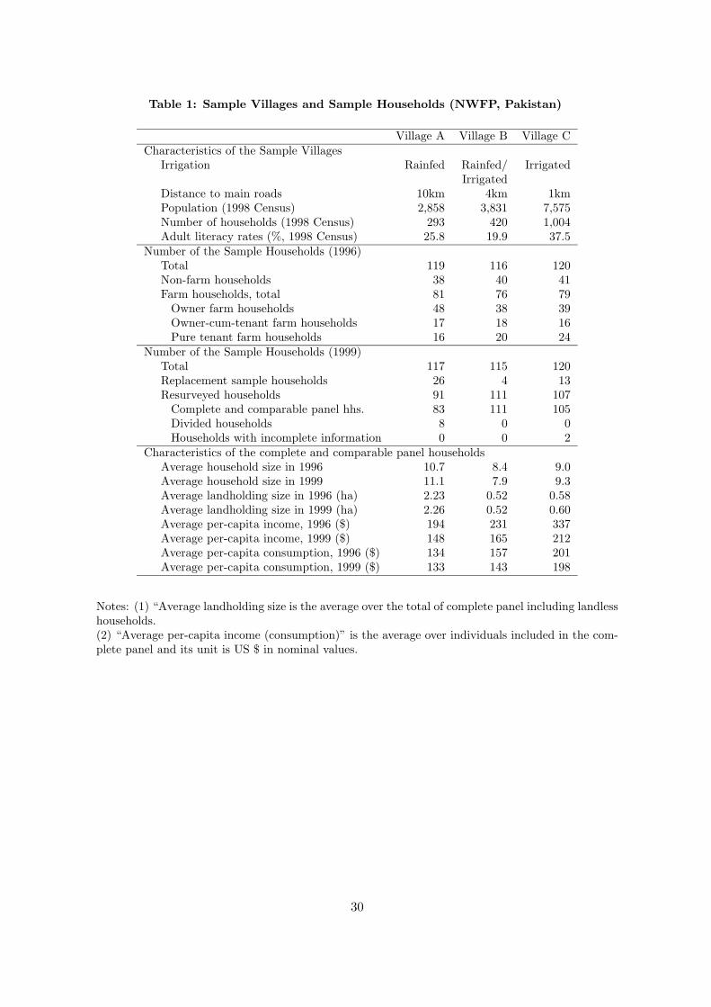
Table 1: Sample Villages and Sample Households (NWFP, Pakistan)
Village A Village B Village C Characteristics of the Sample Villages
Irrigation Rainfed Rainfed/ Irrigated Irrigated
Distance to main roads 10km 4km 1km Population (1998 Census) 2,858 3,831 7,575 Number of households (1998 Census) 293 420 1,004 Adult literacy rates (%, 1998 Census) 25.8 19.9 37.5
Number of the Sample Households (1996) Total 119 116 120 Nonfarm households 38 40 41 Farm households, total 81 76 79
Owner farm households 48 38 39 Ownercumtenant farm households 17 18 16 Pure tenant farm households 16 20 24
Number of the Sample Households (1999) Total 117 115 120 Replacement sample households 26 4 13 Resurveyed households 91 111 107
Complete and comparable panel hhs. 83 111 105 Divided households 8 0 0 Households with incomplete information 0 0 2
Characteristics of the complete and comparable panel households Average household size in 1996 10.7 8.4 9.0 Average household size in 1999 11.1 7.9 9.3 Average landholding size in 1996 (ha) 2.23 0.52 0.58 Average landholding size in 1999 (ha) 2.26 0.52 0.60 Average percapita income, 1996 ($) 194 231 337 Average percapita income, 1999 ($) 148 165 212 Average percapita consumption, 1996 ($) 134 157 201 Average percapita consumption, 1999 ($) 133 143 198
Notes: (1) “Average landholding size is the average over the total of complete panel including landless households. (2) “Average percapita income (consumption)” is the average over individuals included in the complete panel and its unit is US $ in nominal values.
30
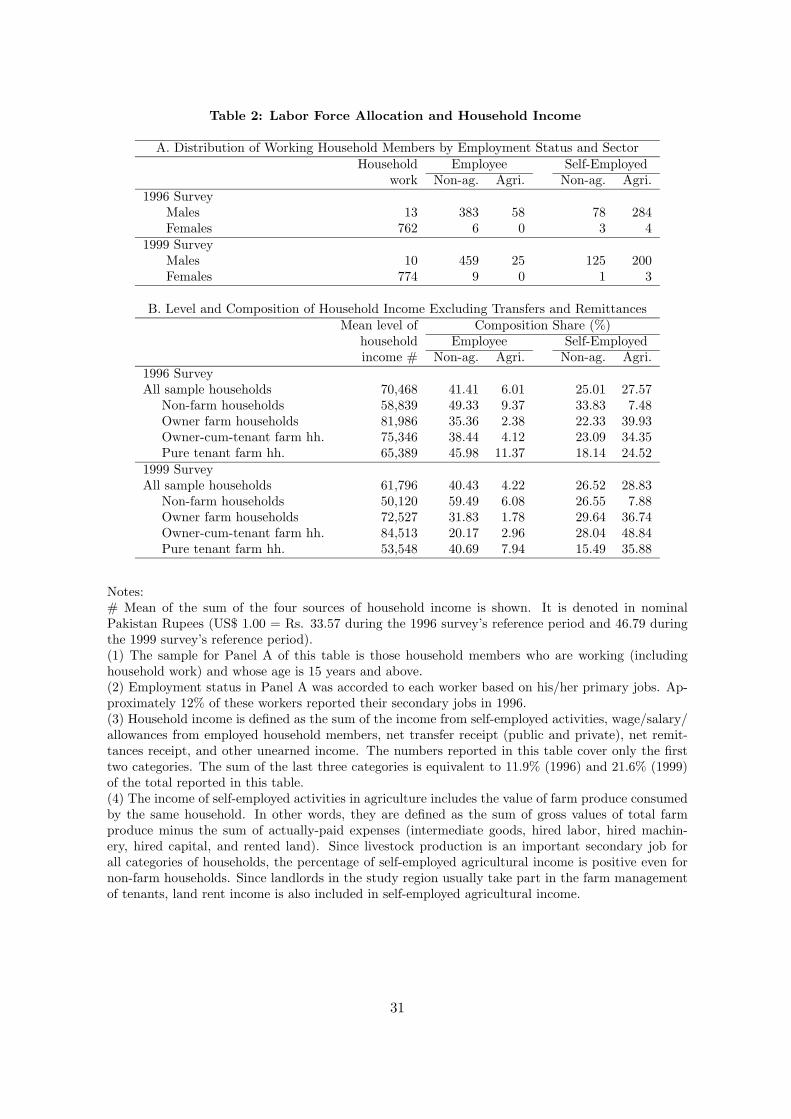
Table 2: Labor Force Allocation and Household Income
A. Distribution of Working Household Members by Employment Status and Sector Household Employee SelfEmployed
work Nonag. Agri. Nonag. Agri. 1996 Survey
Males 13 383 58 78 284 Females 762 6 0 3 4
1999 Survey Males 10 459 25 125 200 Females 774 9 0 1 3
B. Level and Composition of Household Income Excluding Transfers and Remittances Mean level of Composition Share (%)
household income #
Employee Nonag. Agri.
SelfEmNonag.
ployed Agri.
1996 Survey All sample households 70,468 41.41 6.01 25.01 27.57
Nonfarm households 58,839 49.33 9.37 33.83 7.48 Owner farm households 81,986 35.36 2.38 22.33 39.93 Ownercumtenant farm hh. 75,346 38.44 4.12 23.09 34.35 Pure tenant farm hh. 65,389 45.98 11.37 18.14 24.52
1999 Survey All sample households 61,796 40.43 4.22 26.52 28.83
Nonfarm households 50,120 59.49 6.08 26.55 7.88 Owner farm households 72,527 31.83 1.78 29.64 36.74 Ownercumtenant farm hh. 84,513 20.17 2.96 28.04 48.84 Pure tenant farm hh. 53,548 40.69 7.94 15.49 35.88
Notes: # Mean of the sum of the four sources of household income is shown. It is denoted in nominal Pakistan Rupees (US$ 1.00 = Rs. 33.57 during the 1996 survey’s reference period and 46.79 during the 1999 survey’s reference period). (1) The sample for Panel A of this table is those household members who are working (including household work) and whose age is 15 years and above. (2) Employment status in Panel A was accorded to each worker based on his/her primary jobs. Approximately 12% of these workers reported their secondary jobs in 1996. (3) Household income is defined as the sum of the income from selfemployed activities, wage/salary/ allowances from employed household members, net transfer receipt (public and private), net remittances receipt, and other unearned income. The numbers reported in this table cover only the first two categories. The sum of the last three categories is equivalent to 11.9% (1996) and 21.6% (1999) of the total reported in this table. (4) The income of selfemployed activities in agriculture includes the value of farm produce consumed by the same household. In other words, they are defined as the sum of gross values of total farm produce minus the sum of actuallypaid expenses (intermediate goods, hired labor, hired machinery, hired capital, and rented land). Since livestock production is an important secondary job for all categories of households, the percentage of selfemployed agricultural income is positive even for nonfarm households. Since landlords in the study region usually take part in the farm management of tenants, land rent income is also included in selfemployed agricultural income.
31
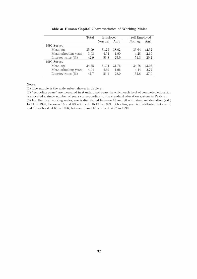
Table 3: Human Capital Characteristics of Working Males
1996 Survey
Total Employee Nonag. Agri.
SelfEmNonag.
ployed Agri.
Mean age 35.99 31.25 38.02 33.64 42.52 Mean schooling years 3.68 4.94 1.90 4.28 2.19 Literacy rates (%) 42.9 53.8 25.9 51.3 29.2
1999 Survey Mean age Mean schooling years Literacy rates (%)
34.55 4.04 47.7
31.04 4.69 53.1
31.76 1.96 28.0
34.78 4.44 52.8
43.05 2.72 37.0
Notes: (1) The sample is the male subset shown in Table 2. (2) “Schooling years” are measured in standardized years, in which each level of completed education is allocated a single number of years corresponding to the standard education system in Pakistan. (3) For the total working males, age is distributed between 15 and 80 with standard deviation (s.d.) 15.11 in 1996; between 15 and 83 with s.d. 15.12 in 1999. Schooling year is distributed between 0 and 16 with s.d. 4.63 in 1996; between 0 and 16 with s.d. 4.67 in 1999.
32
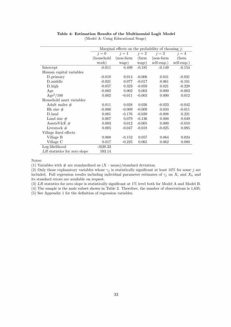
Table 4: Estimation Results of the Multinomial Logit Model (Model A: Using Educational Stage)
Marginal effects on the probability of choosing j: j = 0 j = 1 j = 2 j = 3 j = 4
(household (nonfarm (farm (nonfarm (farm work) wage) wage) selfemp.) selfemp.)
Intercept Human capital variables
D primary D middle D high Age Age2/100
Household asset variables Adult males # Hh size # D land Land size # AssetsV&E # Livestock #
Village fixed effects Village B Village C
0.011
0.018 0.021 0.057 0.002 0.002
0.011 0.006 0.001 0.007 0.003 0.005
0.008 0.017
0.499
0.014 0.077 0.323 0.002
0.011
0.028 0.009 0.176 0.079 0.012 0.047
0.152 0.225
0.185
0.006 0.017 0.059 0.003
0.003
0.026 0.009 0.039 0.136 0.005 0.018
0.057 0.065
0.149 0.154
0.041 0.031 0.061 0.101 0.021 0.228 0.000 0.003 0.000 0.012
0.023 0.042 0.034 0.011
0.008 0.221 0.000 0.049 0.000 0.010
0.025 0.085
0.064 0.024 0.062 0.080
Loglikelihood 1620.33 LR statistics for zero slope 593.14
Notes: (1) Variables with # are standardized as (X mean)/standard deviation. (2) Only those explanatory variables whose γj is statistically significant at least 10% for some j are included. Full regression results including individual parameter estimates of γj on Xi and Xh and its standard errors are available on request. (3) LR statistics for zero slope is statistically significant at 1% level both for Model A and Model B. (4) The sample is the male subset shown in Table 2. Therefore, the number of observations is 1,635. (5) See Appendix 1 for the definition of regression variables.
33
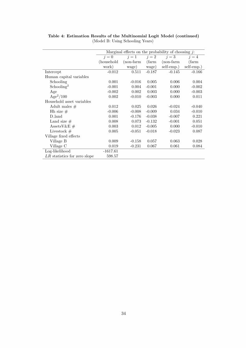
Table 4: Estimation Results of the Multinomial Logit Model (continued) (Model B: Using Schooling Years)
Marginal effects on the probability of choosing j: j = 0 j = 1 j = 2 j = 3 j = 4
(household (nonfarm (farm (nonfarm (farm work) wage) wage) selfemp.) selfemp.)
Intercept Human capital variables
Schooling Schooling2
Age Age2/100
Household asset variables Adult males # Hh size # D land Land size # AssetsV&E # Livestock #
Village fixed effects Village B Village C
0.012
0.001 0.001 0.002 0.002
0.012 0.006 0.001 0.008 0.003 0.005
0.009 0.019
0.511
0.016 0.004 0.002
0.010
0.025 0.008 0.176 0.073 0.012 0.051
0.158 0.231
0.187
0.005 0.001 0.003
0.003
0.026 0.009 0.038 0.132 0.005 0.018
0.057 0.067
0.145 0.166
0.006 0.004 0.000 0.002 0.000 0.003 0.000 0.011
0.024 0.040 0.034 0.010
0.007 0.221 0.001 0.051 0.000 0.010
0.023 0.087
0.063 0.028 0.061 0.084
Loglikelihood 1617.61 LR statistics for zero slope 598.57
34
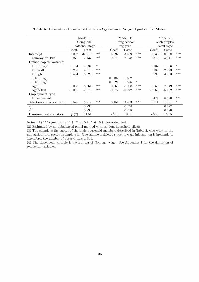
Table 5: Estimation Results of the NonAgricultural Wage Equation for Males
Model A: Model B: Model C: Using edu Using school With employ
cational stage ing year ment type Coeff. tstat Coeff. tstat Coeff. tstat
Intercept 6.002 32.510 *** 6.097 33.659 *** 6.239 30.658 *** Dummy for 1999 0.271 7.137 *** 0.273 7.178 *** 0.310 5.911 ***
Human capital variables D primary 0.154 2.334 ** 0.107 1.686 * D middle 0.268 4.018 *** 0.189 2.973 *** D high 0.494 6.629 *** 0.299 4.993 *** Schooling 0.0182 1.362 Schooling2 0.0021 1.826 * Age 0.068 8.364 *** 0.065 8.068 *** 0.059 7.649 *** Age2/100 0.081 7.276 *** 0.077 6.942 *** 0.063 6.162 ***
Employment type D permanent 0.474 8.570 ***
Selection correction term 0.528 3.919 *** 0.451 3.433 *** 0.211 1.801 * R2 0.236 0.244 0.327 ¯ R2 0.230 0.238 0.320 Hausman test statistics χ2(7) 11.51 χ2(6) 8.31 χ2(8) 13.55
Notes: (1) *** significant at 1%, ** at 5%, * at 10% (twosided test). (2) Estimated by an unbalanced panel method with random household effects. (3) The sample is the subset of the male household members described in Table 2, who work in the nonagricultural sector as employees. One sample is deleted since its wage information is incomplete. Therefore, the number of observations is 841. (4) The dependent variable is natural log of Nonag. wage. See Appendix 1 for the definition of regression variables.
35
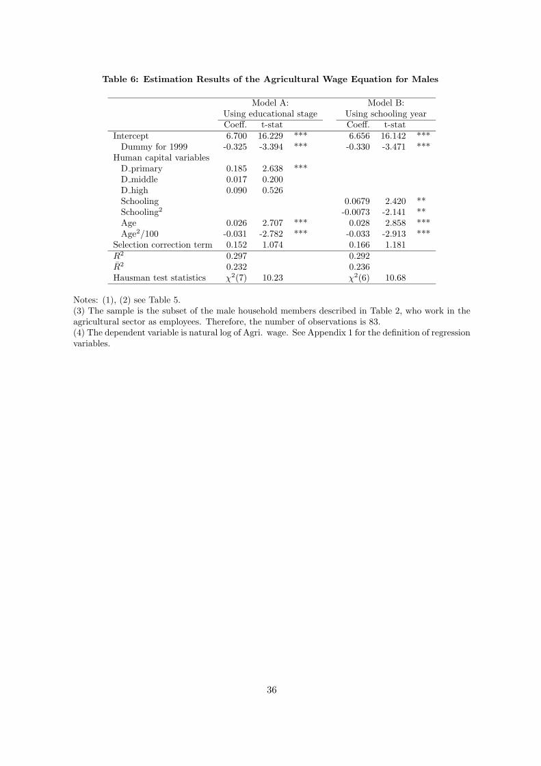
Table 6: Estimation Results of the Agricultural Wage Equation for Males
Model A: Model B: Using educational stage Using schooling year Coeff. tstat Coeff. tstat
Intercept 6.700 16.229 *** 6.656 16.142 *** Dummy for 1999 0.325 3.394 *** 0.330 3.471 ***
Human capital variables D primary 0.185 2.638 *** D middle 0.017 0.200 D high 0.090 0.526 Schooling 0.0679 2.420 ** Schooling2 0.0073 2.141 ** Age 0.026 2.707 *** 0.028 2.858 *** Age2/100 0.031 2.782 *** 0.033 2.913 ***
Selection correction term 0.152 1.074 0.166 1.181 R2 0.297 0.292 ¯ R2 0.232 0.236 Hausman test statistics χ2(7) 10.23 χ2(6) 10.68
Notes: (1), (2) see Table 5. (3) The sample is the subset of the male household members described in Table 2, who work in the agricultural sector as employees. Therefore, the number of observations is 83. (4) The dependent variable is natural log of Agri. wage. See Appendix 1 for the definition of regression variables.
36
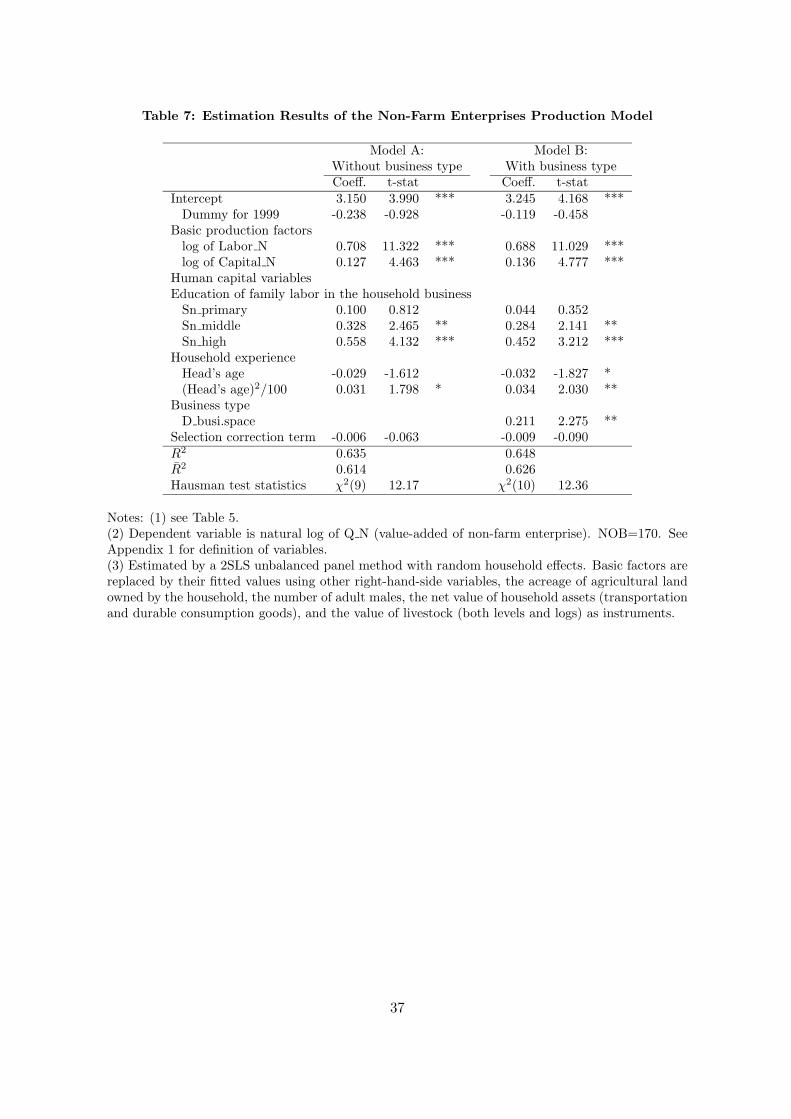
Table 7: Estimation Results of the NonFarm Enterprises Production Model
Model A: Model B: Without business type With business type Coeff. tstat Coeff. tstat
Intercept 3.150 3.990 *** 3.245 4.168 *** Dummy for 1999 0.238 0.928 0.119 0.458
Basic production factors log of Labor N 0.708 11.322 *** 0.688 11.029 *** log of Capital N 0.127 4.463 *** 0.136 4.777 ***
Human capital variables Education of family labor in the household business
Sn primary 0.100 0.812 0.044 0.352 Sn middle 0.328 2.465 ** 0.284 2.141 ** Sn high 0.558 4.132 *** 0.452 3.212 ***
Household experience Head’s age 0.029 1.612 0.032 1.827 * (Head’s age)2/100 0.031 1.798 * 0.034 2.030 **
Business type D busi.space 0.211 2.275 **
Selection correction term 0.006 0.063 0.009 0.090 R2 0.635 0.648 ¯ R2 0.614 0.626 Hausman test statistics χ2(9) 12.17 χ2(10) 12.36
Notes: (1) see Table 5. (2) Dependent variable is natural log of Q N (valueadded of nonfarm enterprise). NOB=170. See Appendix 1 for definition of variables. (3) Estimated by a 2SLS unbalanced panel method with random household effects. Basic factors are replaced by their fitted values using other righthandside variables, the acreage of agricultural land owned by the household, the number of adult males, the net value of household assets (transportation and durable consumption goods), and the value of livestock (both levels and logs) as instruments.
37
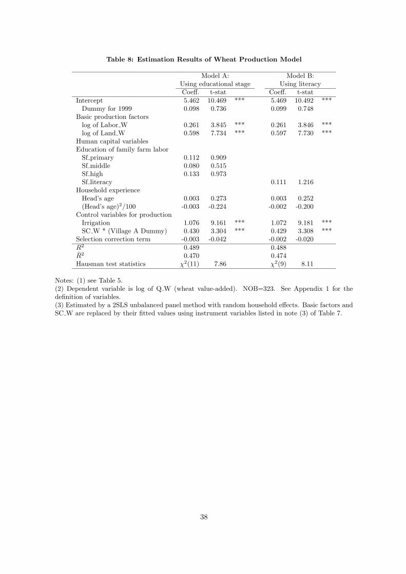
Table 8: Estimation Results of Wheat Production Model
Model A: Model B: Using educational stage Using literacy Coeff. tstat Coeff. tstat 5.462 10.469 *** 5.469 10.492 *** 0.098 0.736 0.099 0.748
0.261 3.845 *** 0.261 3.846 *** 0.598 7.734 *** 0.597 7.730 ***
0.112 0.909 0.080 0.515 0.133 0.973
0.111 1.216
0.003 0.273 0.003 0.252 0.003 0.224 0.002 0.200
1.076 9.161 *** 1.072 9.181 *** 0.430 3.304 *** 0.429 3.308 *** 0.003 0.042 0.002 0.020
Intercept Dummy for 1999
Basic production factors log of Labor W log of Land W
Human capital variables Education of family farm labor
Sf primary Sf middle Sf high Sf literacy
Household experience Head’s age (Head’s age)2/100
Control variables for production Irrigation SC W * (Village A Dummy)
Selection correction term R2 0.489 0.488 ¯ R2 0.470 0.474 Hausman test statistics χ2(11) 7.86 χ2(9) 8.11
Notes: (1) see Table 5. (2) Dependent variable is log of Q W (wheat valueadded). NOB=323. See Appendix 1 for the definition of variables. (3) Estimated by a 2SLS unbalanced panel method with random household effects. Basic factors and SC W are replaced by their fitted values using instrument variables listed in note (3) of Table 7.
38
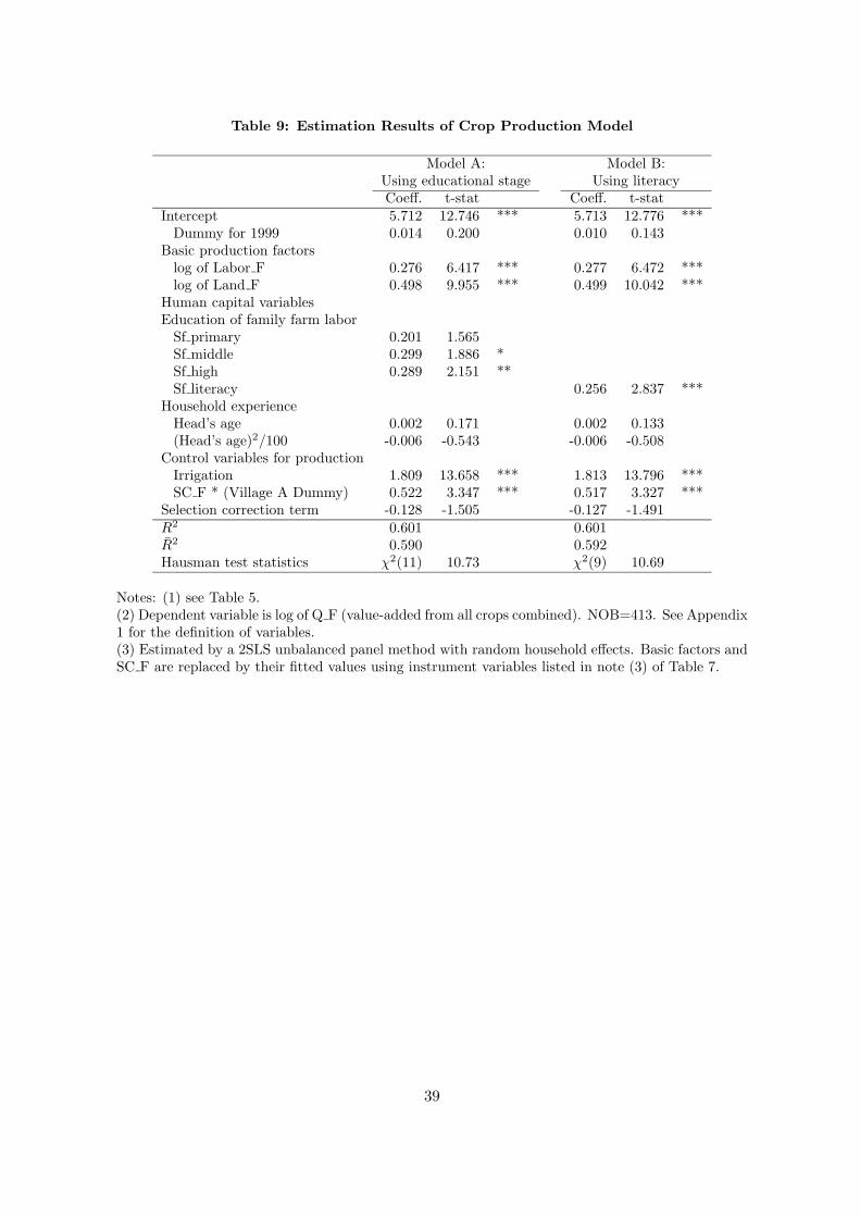
Table 9: Estimation Results of Crop Production Model
Model A: Model B: Using educational stage Using literacy Coeff. tstat Coeff. tstat 5.712 12.746 *** 5.713 12.776 *** 0.014 0.200 0.010 0.143
0.276 6.417 *** 0.277 6.472 *** 0.498 9.955 *** 0.499 10.042 ***
0.201 1.565 0.299 1.886 * 0.289 2.151 **
0.256 2.837 ***
0.002 0.171 0.002 0.133 0.006 0.543 0.006 0.508
1.809 13.658 *** 1.813 13.796 *** 0.522 3.347 *** 0.517 3.327 *** 0.128 1.505 0.127 1.491
Intercept Dummy for 1999
Basic production factors log of Labor F log of Land F
Human capital variables Education of family farm labor
Sf primary Sf middle Sf high Sf literacy
Household experience Head’s age (Head’s age)2/100
Control variables for production Irrigation SC F * (Village A Dummy)
Selection correction term R2 0.601 0.601 ¯ R2 0.590 0.592 Hausman test statistics χ2(11) 10.73 χ2(9) 10.69
Notes: (1) see Table 5. (2) Dependent variable is log of Q F (valueadded from all crops combined). NOB=413. See Appendix 1 for the definition of variables. (3) Estimated by a 2SLS unbalanced panel method with random household effects. Basic factors and SC F are replaced by their fitted values using instrument variables listed in note (3) of Table 7.
39
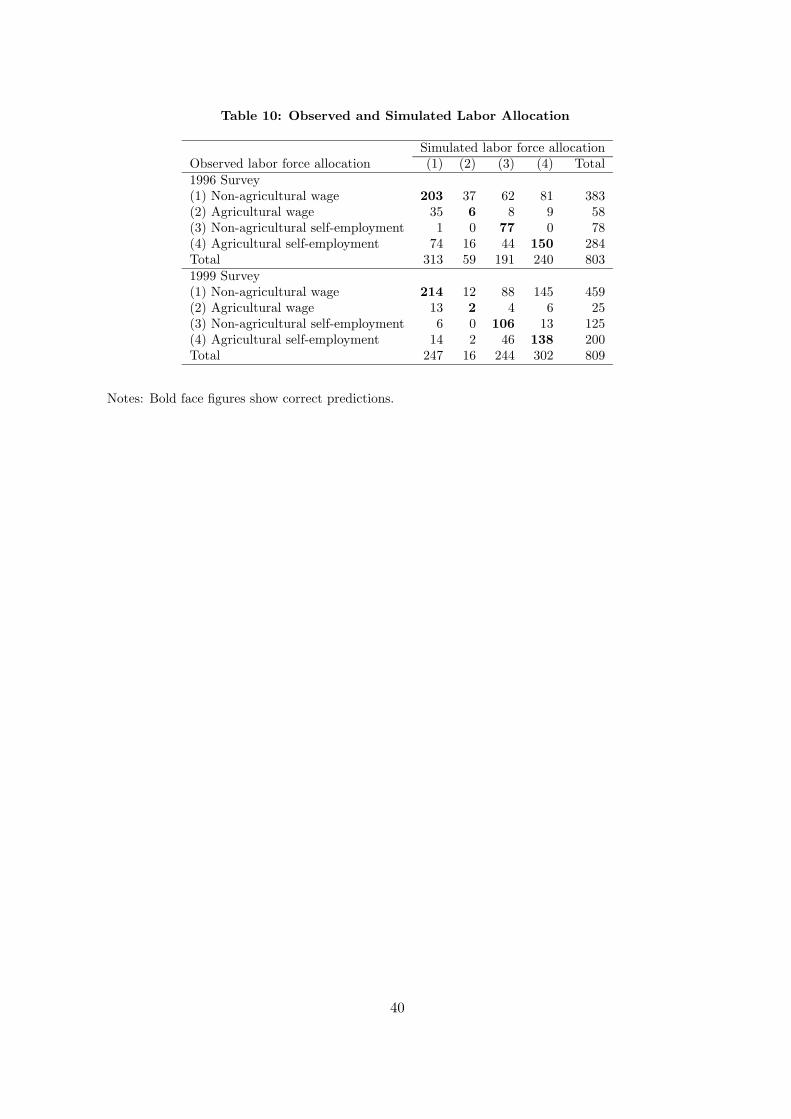
Table 10: Observed and Simulated Labor Allocation
Simulated labor force allocation Observed labor force allocation (1) (2) (3) (4) Total 1996 Survey (1) Nonagricultural wage 203 37 62 81 383 (2) Agricultural wage 35 6 8 9 58 (3) Nonagricultural selfemployment 1 0 77 0 78 (4) Agricultural selfemployment 74 16 44 150 284 Total 313 59 191 240 803 1999 Survey (1) Nonagricultural wage 214 12 88 145 459 (2) Agricultural wage 13 2 4 6 25 (3) Nonagricultural selfemployment 6 0 106 13 125 (4) Agricultural selfemployment 14 2 46 138 200 Total 247 16 244 302 809
Notes: Bold face figures show correct predictions.
40
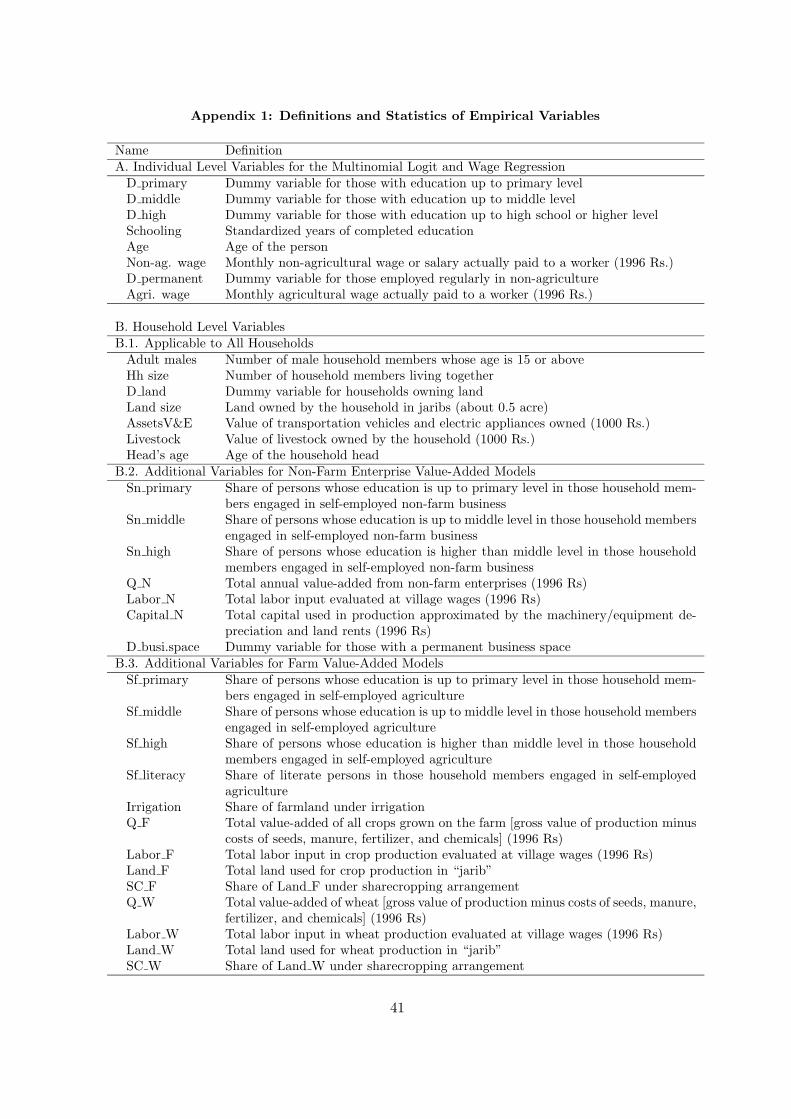
Appendix 1: Definitions and Statistics of Empirical Variables
Name Definition A. Individual Level Variables for the Multinomial Logit and Wage Regression
D primary Dummy variable for those with education up to primary level D middle Dummy variable for those with education up to middle level D high Dummy variable for those with education up to high school or higher level Schooling Standardized years of completed education Age Age of the person Nonag. wage Monthly nonagricultural wage or salary actually paid to a worker (1996 Rs.) D permanent Dummy variable for those employed regularly in nonagriculture Agri. wage Monthly agricultural wage actually paid to a worker (1996 Rs.)
B. Household Level Variables B.1. Applicable to All Households
Adult males Number of male household members whose age is 15 or aboveHh size Number of household members living togetherD land Dummy variable for households owning landLand size Land owned by the household in jaribs (about 0.5 acre)AssetsV&E Value of transportation vehicles and electric appliances owned (1000 Rs.)Livestock Value of livestock owned by the household (1000 Rs.)Head’s age Age of the household head
B.2. Additional Variables for NonFarm Enterprise ValueAdded Models Sn primary Share of persons whose education is up to primary level in those household mem
bers engaged in selfemployed nonfarm business Sn middle Share of persons whose education is up to middle level in those household members
engaged in selfemployed nonfarm business Sn high Share of persons whose education is higher than middle level in those household
members engaged in selfemployed nonfarm business Q N Total annual valueadded from nonfarm enterprises (1996 Rs) Labor N Total labor input evaluated at village wages (1996 Rs) Capital N Total capital used in production approximated by the machinery/equipment de
preciation and land rents (1996 Rs) D busi.space Dummy variable for those with a permanent business space
B.3. Additional Variables for Farm ValueAdded Models Sf primary Share of persons whose education is up to primary level in those household mem
bers engaged in selfemployed agriculture Sf middle Share of persons whose education is up to middle level in those household members
engaged in selfemployed agriculture Sf high Share of persons whose education is higher than middle level in those household
members engaged in selfemployed agriculture Sf literacy Share of literate persons in those household members engaged in selfemployed
agriculture Irrigation Share of farmland under irrigation Q F Total valueadded of all crops grown on the farm [gross value of production minus
costs of seeds, manure, fertilizer, and chemicals] (1996 Rs) Labor F Total labor input in crop production evaluated at village wages (1996 Rs) Land F Total land used for crop production in “jarib” SC F Share of Land F under sharecropping arrangement Q W Total valueadded of wheat [gross value of production minus costs of seeds, manure,
fertilizer, and chemicals] (1996 Rs) Labor W Total labor input in wheat production evaluated at village wages (1996 Rs) Land W Total land used for wheat production in “jarib” SC W Share of Land W under sharecropping arrangement
41
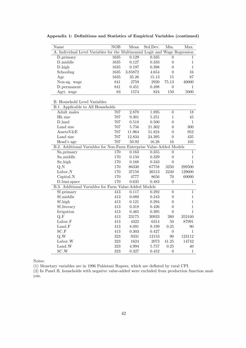
Appendix 1: Definitions and Statistics of Empirical Variables (continued)
Name NOB Mean Std.Dev. Min. Max. A. Individual Level Variables for the Multinomial Logit and Wage Regression
D primary 1635 D middle 1635 D high 1635 Schooling 1635 Age 1635 Nonag. wage 841 D permanent 841 Agri. wage 83
B. Household Level Variables
0.129 0.127 0.197
3.85872 35.26 2759 0.451 1574
0.335 0.333 0.398 4.654 15.13 2920 0.498
824
0 1 0 1 0 1 0 16
15 87 75.13 40000
0 1 150 5000
B.1. Applicable to All Households Adult males 707 2.878 1.895 0 18 Hh size 707 9.301 5.251 1 45 D land 707 0.518 0.500 0 1 Land size 707 5.756 21.302 0 300 AssetsV&E 707 11.964 51.824 0 952 Land size 707 12.834 24.395 0 435 Head’s age 707 50.92 16.28 16 105
B.2. Additional Variables for NonFarm Enterprise ValueAdded Models Sn primary 170 Sn middle 170 Sn high 170 Q N 170 Labor N 170 Capital N 170 D busi.space 170
0.163 0.150 0.168 86330 37158 4777 0.635
0.355 0.329 0.343 67758 26513 8656 0.483
0 1 0 1 0 1
3250 299500 2240 129600
70 60000 0 1
B.3. Additional Variables for Farm ValueAdded Models Sf primary 413 0.117 0.292 0 1 Sf middle 413 0.080 0.243 0 1 Sf high 413 0.121 0.294 0 1 Sf literacy 413 0.318 0.426 0 1 Irrigation 413 0.465 0.395 0 1 Q F 413 23175 30933 260 352440 Labor F 413 4322 6314 50 87991 Land F 413 8.091 9.199 0.25 90 SC F 413 0.303 0.427 0 1 Q W 323 9331 12153 90 123112 Labor W 323 1624 2073 41.25 14742 Land W 323 4.994 5.757 0.25 40 SC W 323 0.327 0.452 0 1
Notes: (1) Monetary variables are in 1996 Pakistani Rupees, which are deflated by rural CPI. (2) In Panel B, households with negative valueadded were excluded from production function analysis.
42
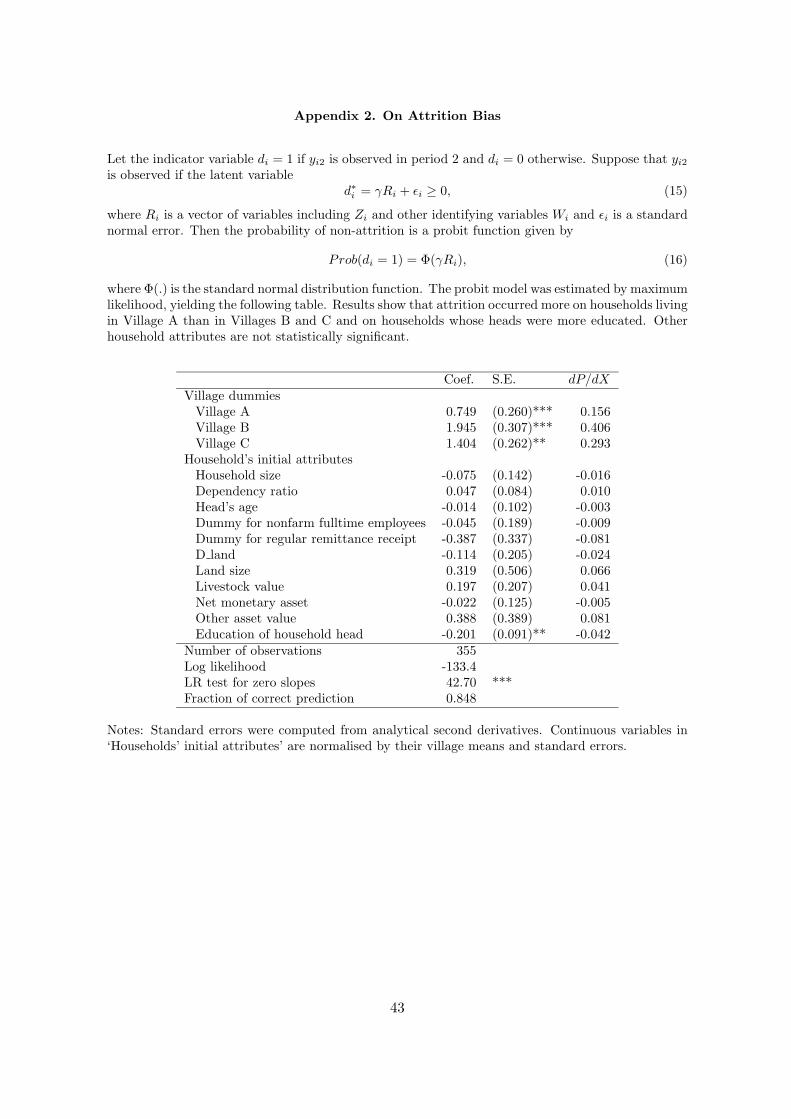
Appendix 2. On Attrition Bias
Let the indicator variable di = 1 if yi2 is observed in period 2 and di = 0 otherwise. Suppose that yi2
is observed if the latent variable d∗ = γRi + �i ≥ 0, (15)i
where Ri is a vector of variables including Zi and other identifying variables Wi and �i is a standard normal error. Then the probability of nonattrition is a probit function given by
Prob(di = 1) = Φ(γRi), (16)
where Φ(.) is the standard normal distribution function. The probit model was estimated by maximum likelihood, yielding the following table. Results show that attrition occurred more on households living in Village A than in Villages B and C and on households whose heads were more educated. Other household attributes are not statistically significant.
Coef. S.E. dP/dX Village dummies
Village A 0.749 (0.260)*** 0.156 Village B 1.945 (0.307)*** 0.406 Village C 1.404 (0.262)** 0.293
Household’s initial attributes Household size 0.075 (0.142) 0.016 Dependency ratio 0.047 (0.084) 0.010 Head’s age 0.014 (0.102) 0.003 Dummy for nonfarm fulltime employees 0.045 (0.189) 0.009 Dummy for regular remittance receipt 0.387 (0.337) 0.081 D land 0.114 (0.205) 0.024 Land size 0.319 (0.506) 0.066 Livestock value 0.197 (0.207) 0.041 Net monetary asset 0.022 (0.125) 0.005 Other asset value 0.388 (0.389) 0.081 Education of household head 0.201 (0.091)** 0.042
Number of observations 355 Log likelihood 133.4 LR test for zero slopes 42.70 *** Fraction of correct prediction 0.848
Notes: Standard errors were computed from analytical second derivatives. Continuous variables in ‘Households’ initial attributes’ are normalised by their village means and standard errors.
43
Recommended