Solving stiffODEs using imexmethods in julia
Kjetil Sonerud
Introduction
What is an imexsolver?
Time scaleanalysis
Numerical solversfor ODE systems
Model
Results
Discussion
Handling stiff ordinary differential equations(ODEs) using imex methods in julia
TKP4555 Process-System Engineering Specialization ModuleTKP11 Advanced Process Simulation
Kjetil Sonerud
Department of Chemical EngineeringNorwegian University of Science and Technology (NTNU)
December 17, 2014
Solving stiffODEs using imexmethods in julia
Kjetil Sonerud
Introduction
What is an imexsolver?
Time scaleanalysis
Numerical solversfor ODE systems
Model
Results
Discussion
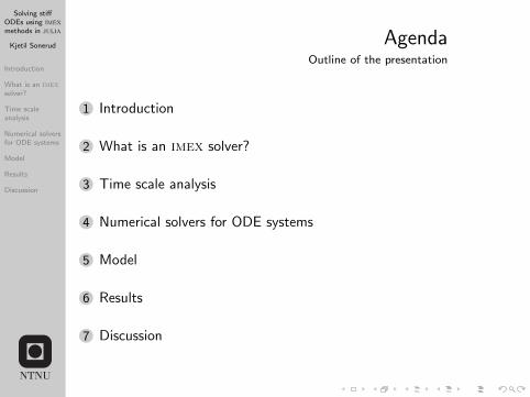
AgendaOutline of the presentation
1 Introduction
2 What is an imex solver?
3 Time scale analysis
4 Numerical solvers for ODE systems
5 Model
6 Results
7 Discussion
Solving stiffODEs using imexmethods in julia
Kjetil Sonerud
Introduction
What is an imexsolver?
Time scaleanalysis
Numerical solversfor ODE systems
Model
Results
Discussion
IntroductionThe role of differential equations
In general, many of the practical problems in science and engineeringmay be formulated as differential equations. Being able to solve these
correctly and efficiently are of great importance to the chemicalengineer.
In practise, many PDEs may be approximated – and all higher-orderODEs may be reduced – to a system of first-order ordinary
differential equations. Thus, the solution of the latter covers a widerange of applications.
We are seldom able to solve the differential equations that are ofpractical interest analytically, so approximating the solution through
the use of numerical methods are often the only viable option.
This is where the issue of stiffness arises. Handling this through theuse of so-called imex methods is the main focus of the current work,
and will be further explained.
Solving stiffODEs using imexmethods in julia
Kjetil Sonerud
Introduction
What is an imexsolver?
Time scaleanalysis
Numerical solversfor ODE systems
Model
Results
Discussion
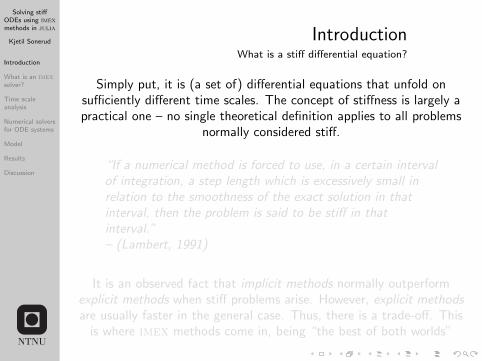
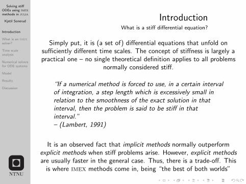
IntroductionWhat is a stiff differential equation?
Simply put, it is (a set of) differential equations that unfold onsufficiently different time scales. The concept of stiffness is largely apractical one – no single theoretical definition applies to all problems
normally considered stiff.
“If a numerical method is forced to use, in a certain intervalof integration, a step length which is excessively small inrelation to the smoothness of the exact solution in thatinterval, then the problem is said to be stiff in thatinterval.”– (Lambert, 1991)
It is an observed fact that implicit methods normally outperformexplicit methods when stiff problems arise. However, explicit methodsare usually faster in the general case. Thus, there is a trade-off. This
is where imex methods come in, being “the best of both worlds”
Solving stiffODEs using imexmethods in julia
Kjetil Sonerud
Introduction
What is an imexsolver?
Time scaleanalysis
Numerical solversfor ODE systems
Model
Results
Discussion
IntroductionWhat is a stiff differential equation?
Simply put, it is (a set of) differential equations that unfold onsufficiently different time scales. The concept of stiffness is largely apractical one – no single theoretical definition applies to all problems
normally considered stiff.
“If a numerical method is forced to use, in a certain intervalof integration, a step length which is excessively small inrelation to the smoothness of the exact solution in thatinterval, then the problem is said to be stiff in thatinterval.”– (Lambert, 1991)
It is an observed fact that implicit methods normally outperformexplicit methods when stiff problems arise. However, explicit methodsare usually faster in the general case. Thus, there is a trade-off. This
is where imex methods come in, being “the best of both worlds”

Solving stiffODEs using imexmethods in julia
Kjetil Sonerud
Introduction
What is an imexsolver?
Time scaleanalysis
Numerical solversfor ODE systems
Model
Results
Discussion
IntroductionAn illustrative example
0 2 4 6 8 10
0
0.2
0.4
0.6
0.8
1
y
Analytic solution
0 2 4 6 8 10
0
0.2
0.4
0.6
0.8
1
t [sec]
IM Euler with ∆t = 1 s
0 2 4 6 8 10
0
0.2
0.4
0.6
0.8
1·1016
EX Euler with ∆t = 1 s
Comparing IM- and EX Euler with the analytic solution
Figure: Comparison of the analytic solution to those of ex Euler and imEuler method for the ODE-system described in y ′′ + 101y ′ + 100y = 0.The time step is ∆t = 1 s. Note that the im Euler solution is quite close tothe analytical, but that the ex Euler method fails spectacularly.

Solving stiffODEs using imexmethods in julia
Kjetil Sonerud
Introduction
What is an imexsolver?
Time scaleanalysis
Numerical solversfor ODE systems
Model
Results
Discussion
IntroductionAn illustrative example
0 2 4 6 8 10
0
0.2
0.4
0.6
0.8
1
y
Analytic solution
0 2 4 6 8 10
0
0.2
0.4
0.6
0.8
1
t [sec]
IM Euler with ∆t = 1 × 10⁻³ s
0 2 4 6 8 10
0
0.2
0.4
0.6
0.8
1
EX Euler with ∆t = 1 × 10⁻³ s
Comparing IM- and EX Euler with the analytic solution
Figure: Comparison of the analytic solution to those of ex Euler and imEuler method for the ODE-system described in y ′′ + 101y ′ + 100y = 0.The time step is ∆t = 1 × 10⁻³ s. Now, both ex Euler and im Euler arevery close to the actual analytic solution.

Solving stiffODEs using imexmethods in julia
Kjetil Sonerud
Introduction
What is an imexsolver?
Time scaleanalysis
Numerical solversfor ODE systems
Model
Results
Discussion
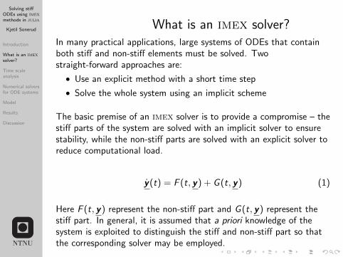
What is an imex solver?In many practical applications, large systems of ODEs that containboth stiff and non-stiff elements must be solved. Twostraight-forward approaches are:
• Use an explicit method with a short time step
• Solve the whole system using an implicit scheme
The basic premise of an imex solver is to provide a compromise – thestiff parts of the system are solved with an implicit solver to ensurestability, while the non-stiff parts are solved with an explicit solver toreduce computational load.
y(t) = F (t, y) + G (t, y) (1)
Here F (t, y) represent the non-stiff part and G (t, y) represent thestiff part. In general, it is assumed that a priori knowledge of thesystem is exploited to distinguish the stiff and non-stiff part so thatthe corresponding solver may be employed.

Solving stiffODEs using imexmethods in julia
Kjetil Sonerud
Introduction
What is an imexsolver?
Time scaleanalysis
Numerical solversfor ODE systems
Model
Results
Discussion
What is an imex solver?In many practical applications, large systems of ODEs that containboth stiff and non-stiff elements must be solved. Twostraight-forward approaches are:
• Use an explicit method with a short time step
• Solve the whole system using an implicit scheme
The basic premise of an imex solver is to provide a compromise – thestiff parts of the system are solved with an implicit solver to ensurestability, while the non-stiff parts are solved with an explicit solver toreduce computational load.
y(t) = F (t, y) + G (t, y) (1)
Here F (t, y) represent the non-stiff part and G (t, y) represent thestiff part. In general, it is assumed that a priori knowledge of thesystem is exploited to distinguish the stiff and non-stiff part so thatthe corresponding solver may be employed.

Solving stiffODEs using imexmethods in julia
Kjetil Sonerud
Introduction
What is an imexsolver?
Time scaleanalysis
Numerical solversfor ODE systems
Model
Results
Discussion
Time scale analysisAlternative strategies for solving stiff equations
Event Dynamic Constant
t
Small timescales
Large timescales
Figure: Illustration of time scales: the dynamic time scale is flanked to theleft by the small time scales, which may be considered like events. To theright, the dynamic time scale is flanked by the large time scales, which maybe considered constant.
Solving stiffODEs using imexmethods in julia
Kjetil Sonerud
Introduction
What is an imexsolver?
Time scaleanalysis
Numerical solversfor ODE systems
Model
Results
Discussion
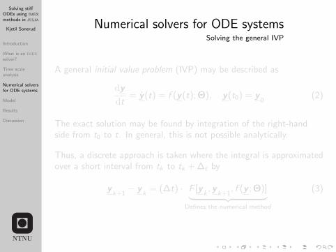
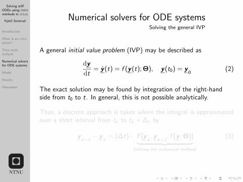
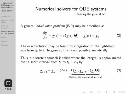
Numerical solvers for ODE systemsSolving the general IVP
A general initial value problem (IVP) may be described as
dydt
= y(t) = f (y(t); Θ), y(t0) = y0
(2)
The exact solution may be found by integration of the right-handside from t0 to t. In general, this is not possible analytically.
Thus, a discrete approach is taken where the integral is approximatedover a short interval from tk to tk + ∆t by
yk+1− y
k= (∆t) · F [y
k, y
k+1, f (y ; Θ)]︸ ︷︷ ︸
Defines the numerical method
(3)

Solving stiffODEs using imexmethods in julia
Kjetil Sonerud
Introduction
What is an imexsolver?
Time scaleanalysis
Numerical solversfor ODE systems
Model
Results
Discussion
Numerical solvers for ODE systemsSolving the general IVP
A general initial value problem (IVP) may be described as
dydt
= y(t) = f (y(t); Θ), y(t0) = y0
(2)
The exact solution may be found by integration of the right-handside from t0 to t. In general, this is not possible analytically.
Thus, a discrete approach is taken where the integral is approximatedover a short interval from tk to tk + ∆t by
yk+1− y
k= (∆t) · F [y
k, y
k+1, f (y ; Θ)]︸ ︷︷ ︸
Defines the numerical method
(3)
Solving stiffODEs using imexmethods in julia
Kjetil Sonerud
Introduction
What is an imexsolver?
Time scaleanalysis
Numerical solversfor ODE systems
Model
Results
Discussion
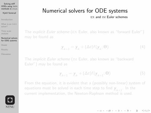
Numerical solvers for ODE systemsex and im Euler schemes
The explicit Euler scheme (ex Euler, also known as “forward Euler”)may be found as
yk+1
= yk
+ (∆t)f (yk; Θ) (4)
The implicit Euler scheme (im Euler, also known as “backwardEuler”) may be found as
yk+1
= yk
+ (∆t)f (yk+1
; Θ) (5)
From the equation, it is evident that a (possibly non-linear) system ofequations must be solved in each time step to find y
k+1. In the
current implementation, the Newton-Raphson method is used.

Solving stiffODEs using imexmethods in julia
Kjetil Sonerud
Introduction
What is an imexsolver?
Time scaleanalysis
Numerical solversfor ODE systems
Model
Results
Discussion
Numerical solvers for ODE systemsThe imex Euler scheme
With the assumption that the system of ODEs are readily split intoan implicit part and an explicit part, the imex Euler scheme followsy IM
k+1
yEXk+1
=
y IMk
yEXk
+ ∆t
f (y IMk+1
, yEXk+1
; Θ)
f (yEXk
; Θ)
(6)
Note that to solve for y IMk+1
, it is necessary to first solve for yEXk+1
, as
the latter is used in the solution of the former. Thus, in theNewton-Raphson iteration to solve for y IM
k+1, it is assumed that yEX
k+1is constant during the course of the iterations.

Solving stiffODEs using imexmethods in julia
Kjetil Sonerud
Introduction
What is an imexsolver?
Time scaleanalysis
Numerical solversfor ODE systems
Model
Results
Discussion
ModelThe original Robertson kinetic problem
“When the equations represent the behaviour of a systemcontaining a number of fast and slow reactions, a forwardintegration of these equations becomes difficult.”– (Robertson, 1966)
The original problem as stated by Robertson is one of anautocatalytic reaction
A0.04−−→ B (slow) (7a)
B + B3·107
−−−→ C + B (very fast) (7b)
B + C1·104
−−−→ A + C (fast) (7c)
Note that the reaction rate constants differ with several orders ofmagnitude, which we might suspect – correctly, as it turns out –makes the system stiff.
Solving stiffODEs using imexmethods in julia
Kjetil Sonerud
Introduction
What is an imexsolver?
Time scaleanalysis
Numerical solversfor ODE systems
Model
Results
Discussion
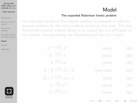
ModelThe expanded Robertson kinetic problem
An expanded version of the original problem is proposed in order topromote solution by the imex method central to this work. The ideabehind the reaction scheme shown is to expand the non-stiff parts ofthe system, thus promoting the effectiveness of the imex solver.
A?? 0.03−−→ A? (slow) (8a)
A? 0.05−−→ A (slow) (8b)
A0.04−−→ B (slow) (8c)
B + B3·107
−−−→ C + B (very fast) (8d)
B + C1·104
−−−→ A + C (fast) (8e)
C0.05−−→ C? (slow) (8f)
C? 0.04−−→ C?? (slow) (8g)

Solving stiffODEs using imexmethods in julia
Kjetil Sonerud
Introduction
What is an imexsolver?
Time scaleanalysis
Numerical solversfor ODE systems
Model
Results
Discussion
ResultsOriginal Robertson problem
0 10 20 30 40
0.7
0.8
0.9
1
Molefraction
[-]
A
0 10 20 30 40
0.0 · 100
1.0 · 10−5
2.0 · 10−5
3.0 · 10−5
t [sec]
B
0 10 20 30 40
0
0.1
0.2
0.3C
Solving the original Robertson problem with an IMEX Euler solver
Figure: Solving the Robertson kinetics problem – original version – withimex Euler. The step size in this case is ∆t = 1 s.
Solving stiffODEs using imexmethods in julia
Kjetil Sonerud
Introduction
What is an imexsolver?
Time scaleanalysis
Numerical solversfor ODE systems
Model
Results
Discussion
ResultsOriginal Robertson problem
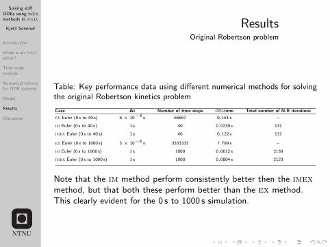
Table: Key performance data using different numerical methods for solvingthe original Robertson kinetics problem
Case ∆t Number of time steps CPU-time Total number of N-R iterations
ex Euler (0 s to 40 s) 6 × 10⁻⁴ s 66667 0.161 s –
im Euler (0 s to 40 s) 1 s 40 0.0239 s 131
imex Euler (0 s to 40 s) 1 s 40 0.122 s 131
ex Euler (0 s to 1000 s) 3 × 10⁻⁴ s 3333333 7.789 s –
im Euler (0 s to 1000 s) 1 s 1000 0.0612 s 2138
imex Euler (0 s to 1000 s) 1 s 1000 0.0804 s 2123
Note that the im method perform consistently better then the imexmethod, but that both these perform better than the ex method.This clearly evident for the 0 s to 1000 s simulation.

Solving stiffODEs using imexmethods in julia
Kjetil Sonerud
Introduction
What is an imexsolver?
Time scaleanalysis
Numerical solversfor ODE systems
Model
Results
Discussion
ResultsOriginal Robertson problem
38 38.5 39 39.5 400.71
0.71
0.72
0.72
0.72
Molefraction
[-]
A
38 38.5 39 39.5 40
−5.0 · 10−6
0.0 · 100
5.0 · 10−6
1.0 · 10−5
1.5 · 10−5
2.0 · 10−5
t [sec]
B
38 38.5 39 39.5 40
0.28
0.28
0.28
0.29
0.29C
Solving the original Robertson problem with an EX Euler solver
Figure: Solving the Robertson kinetics problem – original version – with exEuler. The emerging stability problem when calculating the B-trajectoryare evident.

Solving stiffODEs using imexmethods in julia
Kjetil Sonerud
Introduction
What is an imexsolver?
Time scaleanalysis
Numerical solversfor ODE systems
Model
Results
Discussion
ResultsExpanded Robertson problem
0 200 400 600
0
0.2
0.4
0.6
0.8
1Molefraction
[-]
A??
A?
ACC?
C??
0 200 400 600
0
0.5
1
·10−5
B
Solving the expanded Robertson problem with an IMEX Euler solver
t [sec]
Figure: Solving the Robertson kinetics problem – expanded version – withan IMEX Euler for the time interval 0 s to 600 s. The step size in this caseis ∆t = 1 s.

Solving stiffODEs using imexmethods in julia
Kjetil Sonerud
Introduction
What is an imexsolver?
Time scaleanalysis
Numerical solversfor ODE systems
Model
Results
Discussion
ResultsExpanded Robertson problem
Table: Key performance data using different numerical methods for solvingthe expanded Robertson kinetics problem
Case ∆t Number of time steps CPU-time Total number of N-R iterations
ex Euler (0 s to 600 s) 1 × 10⁻³ s 600000 2.160 s –
im Euler (0 s to 600 s) 1 s 600 0.0533 s 1471
imex Euler (0 s to 600 s) 1 s 600 0.143 s 2506
0 100 200 300 400 500 600
0
2
4
6
8
Mean number ofiterations ≈ 2.45
Number
ofiterations
IM Euler solver
0 100 200 300 400 500 600
0
2
4
6
8
Mean number ofiterations ≈ 4.18
IMEX Euler solver
Number of N-R iterations at each time step
t [sec]
Solving stiffODEs using imexmethods in julia
Kjetil Sonerud
Introduction
What is an imexsolver?
Time scaleanalysis
Numerical solversfor ODE systems
Model
Results
Discussion
Discussion
From the results, it seems evident that the current imex Eulerimplementation is less effective than the pure im Eulerimplementation on the current model system. This may be due toseveral factors:
• Sub-optimal implementation of the imex solver
• The system is not sufficiently large (more precisely, the non-stiffpart is relatively too small) to fully exploit the imex scheme
• The added benefit of solving the whole system implicitly in juliaoutweighs the added cost of solving a larger system of equations
Thus, further work should be done to investigate
• Better imex implementations, possibly with non-Euler methods
• Larger systems of ODEs, especially ones with a small stiff and alarge non-stiff part
Recommended