Ground Truth Bias in External Cluster Validity Indices
Yang Leia,∗, James C. Bezdeka, Simone Romanoa, Nguyen Xuan Vinha, JeffreyChanb, James Baileya
aDepartment of Computing and Information SystemsThe University of Melbourne, Victoria, Australia
bSchool of Science (Computer Science and Information Technology)RMIT University, Victoria, Australia
Abstract
External cluster validity indices (CVIs) are used to quantify the quality of a
clustering by comparing the similarity between the clustering and a ground
truth partition. However, some external CVIs show a biased behavior when
selecting the most similar clustering. Users may consequently be misguided
by such results. Recognizing and understanding the bias behavior of CVIs is
therefore crucial.
It has been noticed that, some external CVIs exhibit a preferential bias
towards a larger or smaller number of clusters which is monotonic (directly or
inversely) in the number of clusters in candidate partitions. This type of bias
is caused by the functional form of the CVI model. For example, the popular
Rand Index (RI) exhibits a monotone increasing (NCinc) bias, while the Jaccard
Index (JI) index suffers from a monotone decreasing (NCdec) bias. This type
of bias has been previously recognized in the literature.
In this work, we identify a new type of bias arising from the distribution
of the ground truth (reference) partition against which candidate partitions are
compared. We call this new type of bias ground truth (GT) bias. This type
of bias occurs if a change in the reference partition causes a change in the bias
∗Corresponding authorEmail addresses: [email protected] (Yang Lei), [email protected]
(James C. Bezdek), [email protected] (Simone Romano),[email protected] (Nguyen Xuan Vinh), [email protected] (JeffreyChan), [email protected] (James Bailey)
Preprint submitted to Pattern Recognition October 14, 2016
status (e.g., NCinc, NCdec) of a CVI. For example, NCinc bias in the RI can
be changed to NCdec bias by skewing the distribution of clusters in the ground
truth partition. It is important for users to be aware of this new type of biased
behavior, since it may affect the interpretations of CVI results.
The objective of this article is to study the empirical and theoretical impli-
cations of GT bias. To the best of our knowledge, this is the first extensive
study of such a property for external CVIs. Our computational experiments
show that 5 of 26 pair-counting based CVIs studied in this paper, which are
all functions of the RI, exhibit GT bias. Following the numerical examples, we
provide a theoretical analysis of GT bias based on the relationship between the
RI and quadratic entropy. Specifically, we prove that the quadratic entropy of
the ground truth partition provides a computable test which predicts the NC
bias status of the RI.
Keywords: External Cluster Validity Indices, Rand Index, Ground Truth
Bias, Quadratic Entropy
1. Introduction
Clustering is one of the fundamental techniques in data mining, which helps
users explore potentially interesting patterns in unlabeled data. Cluster anal-
ysis has been widely used in many areas, ranging from bioinformatics [1] and
market segmentation [2] to information retrieval [3] and image processing [4].5
However, depending on different factors, e.g., different clustering algorithms,
initializations, parameter settings (the number of clusters c), many alternative
candidate partitions might be discovered for a fixed dataset.
Cluster validity indices (CVIs) are used to quantify the goodness of a parti-
tion. Many CVIs have been proposed and successfully used for this task [5, 6,10
7, 8]. These measures can be generally divided into two major types: internal
and external. If the data are labeled, the ground truth partition can be used
with an external CVI to explore the match between candidate and ground truth
partitions. Since the labeled data may not correspond to clusters proposed by
2
any algorithm, we will refer groups in the ground truth as subsets, and algo-15
rithmically proposed groups as clusters. When the data are unlabeled (the real
case), an important post-clustering question is how to evaluate different candi-
date partitions. This job falls to the internal CVIs. One of the most important
uses of the external CVIs is to evaluate the comparative quality of internal CVIs
on labeled data [9], so that in the real case, some confidence can be placed in20
a chosen internal CVI to guide us towards realistic clusters found in unlabeled
data. This article is focused on external CVIs.
External CVIs (or comparison measures), are often interpreted as similarity
(or dissimilarity) measures between the ground truth and candidate partitions.
The ground truth partition, which is usually generated by an expert in the25
data domain, identifies the primary substructure of interest to the expert. This
partition provides a benchmark for comparison with candidate partitions. The
general idea of this evaluation methodology is that the more similar a candidate
is to the ground truth (a larger value for the similarity measure), the better this
partition approximates the labeled structure in the data.30
However, this evaluation methodology implicitly assumes that the similarity
measure works correctly, i.e., that a larger similarity score indicates a partition
that is really more similar to the ground truth. But this assumption may not
always hold. When this assumption is false, the evaluation results will be mis-
leading. One of the reasons that can cause the assumption to be false is that35
a measure may have bias issues. That is, some measures are biased towards
certain clusterings, even though they are not more similar to the ground truth
compared to the other candidate partitions being evaluated. This can cause
misleading results for users employing these biased measures. Thus, recogniz-
ing and understanding the bias behavior of the CVIs is crucial.40
The Rand Index (RI, similarity measure) is a very popular pair-counting
based validation measure that has been widely used in many applications [10,
11, 12, 13, 14, 15, 16] in the last five years. It has been noticed that the RI tends
to favor candidate partitions with larger numbers of clusters when the number
of subsets in the ground truth is fixed [5], i.e., it tends to increase as the number45
3
of clusters increases (we call it NCinc bias in this work, where NC = number of
clusters). NC bias means that the CVI’s preference is influenced by the number
of clusters in the candidate partitions. For example, some measures may prefer
the partition with larger (smaller) number of clusters, i.e., NCinc (NCdec) bias.
The following initial example illustrates NC bias for two popular measures, the50
Rand Index (RI) and Jaccard Index (JI) measures.
1.1. Example 1 - NC bias of RI and JI
In this example, we illustrate NC bias for RI and JI. We generate a set of
candidate partitions randomly with different numbers of clusters and a random
ground truth. We use RI and JI to choose the most similar partition from55
the candidate partitions by comparing the similarity between each of them and
the ground truth. As there is no difference in the generation methodology of
the candidate partitions, we expect them to be treated equally on average.
A measure without NC bias should treat these candidate partitions equally
without preference to any partition in terms of their different number of clusters.60
However, if a measure prefers the partition, e.g., with a larger number of clusters
(gives higher value to the partition with a larger number of clusters if it is a
similarity measure), we say it possess NC bias, more specifically, NCinc bias.
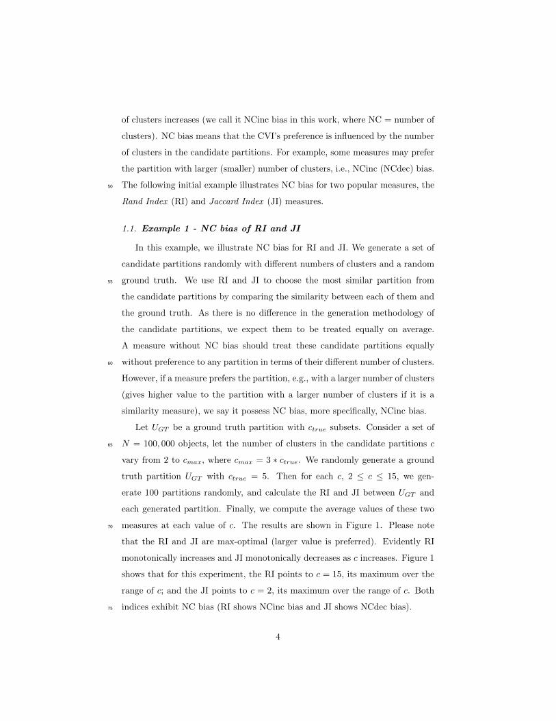
Let UGT be a ground truth partition with ctrue subsets. Consider a set of
N = 100, 000 objects, let the number of clusters in the candidate partitions c65
vary from 2 to cmax, where cmax = 3 ∗ ctrue. We randomly generate a ground
truth partition UGT with ctrue = 5. Then for each c, 2 ≤ c ≤ 15, we gen-
erate 100 partitions randomly, and calculate the RI and JI between UGT and
each generated partition. Finally, we compute the average values of these two
measures at each value of c. The results are shown in Figure 1. Please note70
that the RI and JI are max-optimal (larger value is preferred). Evidently RI
monotonically increases and JI monotonically decreases as c increases. Figure 1
shows that for this experiment, the RI points to c = 15, its maximum over the
range of c; and the JI points to c = 2, its maximum over the range of c. Both
indices exhibit NC bias (RI shows NCinc bias and JI shows NCdec bias).75
4
2 4 6 8 10 12 14
Ave
rage
Val
ues
of In
dex
0
0.1
0.2
0.3
0.4
0.5
0.6
0.7RI"
# Clusters in Candidate Partitions
(a) Average RI values with random
UGT containing 5 subsets.
2 4 6 8 10 12 14
Ave
rage
Val
ues
of In
dex
0
0.05
0.1
0.15Jaccard"
# Clusters in Candidate Partitions
(b) Averge JI values with random UGT
containing 5 subsets.
Figure 1: The average RI and JI values over 100 partitions at each c with uniformly generated
ground truth. The symbol ↑ means larger values are preferred. Vertical line indicates correct
number of clusters.
2 4 6 8 10 12 14
Ave
rage
Val
ues
of In
dex
0
0.1
0.2
0.3
0.4
0.5
RI"
# Clusters in Candidate Partitions
(a) Average RI values with skewed
ground truth.
Cluster#2 4 6 8 10 12 14
Ave
rage
Val
ues
of In
dex
0
0.05
0.1
0.15
0.2
0.25
0.3
0.35Jaccard"
(b) Averge JI values with skewed
ground truth.
Figure 2: The average RI and JI values over 100 partitions at each c with skewed ground
truth. The symbol ↑ means larger values are preferred. Vertical line indicates correct number
of clusters.
But, does the RI always exhibit NCinc bias towards clusterings with a larger
numbers of clusters? The answer is no. We have discovered that the overall bias
of some CVIs, including the RI, may change their NC bias tendencies depending
on the distribution of the subsets in the ground truth. The change in the NC
bias status of an external CVI due to the different ground truths is called GT80
bias. This kind of changeable bias behavior caused by the ground truth has not
been recognized previously in the literature. It is important to be aware of this
5
phenomenon, since it affects how a user should interpret clustering validation
results. Next, we give an example of GT bias (GT = ground truth).
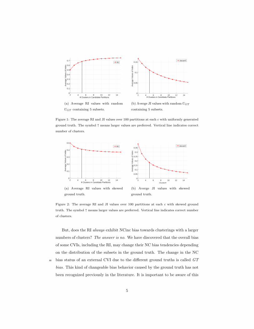
1.2. Example 2 - GT bias of RI85
We use the same protocols as in Example 1, but change the distribution of
the subsets in the ground truth by randomly assigning 80% of the objects to
the first cluster and then randomly assigning the remaining 20% of the labels
to the other four clusters for c = 2, 3, 4, 5. Thus, the distribution of the ground
truth is heavily skewed (non-uniform). The average values of RI and JI are90
shown in Figure 2. The shape of JI in Figures 1b and 2b is same: it still
decreases monotonically with c, exhibiting NCdec bias, and indicating c = 2 as
its preferred choice. Turning now to the RI, we see that trend seen in Figure 1a is
reversed. The RI in Figure 2a is maximum at c = 2, and decreases monotonically
as c increases. So the NC bias of RI has changed from NCinc bias to NCdec95
bias. Thus, RI shows GT bias. To summarize, Examples 1 and 2 show that
NC bias is possessed by some external CVIs due to monotonic tendencies of the
underlying mathematical model. But beyond this, some external CVIs can be
influenced by GT bias, which is due to the way the distribution of the ground
truth interacts with the elements of the CVI.100
The objective of this article is to study the empirical and theoretical impli-
cations of GT bias. To the best of our knowledge, this is the first extensive
study of this property for external cluster validity indices. In this work, our
contributions can be summarized as follows:
1. We identify the GT bias effect for external validation measures, and also105
explain its importance.
2. We test and discuss NC bias for 26 popular pair-counting based external
validation measures.
3. We prove that RI and related 4 indices suffer from GT bias. And also
provide theoretical explanations for understanding why GT bias happens110
and when it happens on RI and related 4 indices.
4. We present experimental results that support our analysis.
6
5. We present an empirical example to show that Adjusted Rand index (ARI)
also suffers from a modified GT bias.
The remainder of the paper is organized as follows. In Section 2 we discuss115
work related to the bias problems of some external validation measures. We
introduce relevant notations and definitions of NC bias and GT bias in Section 3.
In Section 4, we briefly introduce some background knowledge about 26 pair-
counting based external validation measures. In section 5, we test the influence
of NC bias and GT bias for these 26 measures. Theoretical analysis of GT bias120
on the RI is presented in Section 6. An experimental example, showing that
ARI has GT bias in certain scenarios, is presented in Section 7. The paper is
concluded in Section 8.
2. Related Work
Several works have discussed the bias behavior of external CVIs. As the125
conditions imposed on the discussion of the biased behavior are varied, here
we classify these conditions into three categories for convenience of discussion:
i) general bias; ii) NC bias; iii) GT bias.
General Bias. It has been noticed that the RI exhibits a monotonic trend as
both the number of subsets in the ground truth and the number of clusters in130
the candidate partitions increases [17, 18, 19]. However, in our case, we consider
the monotonic bias behavior of an external CVI as a function of the number of
clusters in the candidate partitions when the number of subsets in the ground
truth is fixed.
Wu et al. [20] observed that some external CVIs were unduly influenced135
by the well known tendency of k-means to equalize cluster sizes. They noted
that certain CVIs tended to prefer approximately balanced k-means solutions
even though the ground truth distribution was heavily skewed. The only case
considered in [20] was the special case when all of the candidate partitions
had the same number of clusters. We will develop the general case, allowing140
candidate partitions to have different numbers of clusters.
7
Wu et al. [21] studied the use of the external CVI known as the F-measure for
evaluation of clusters in the context of document retrieval. They found that the
F-measure tends to assign higher scores to partitions containing a large number
of clusters, which they called the “the incremental effect” of the F-measure.145
These authors also found that the F-measure has a “prior-probability effect”,
i.e., the F-measure tends to assign higher scores to partitions with higher prior
probabilities for the relevant documents. Wu et al. only discussed using the
F-measure for accepting or rejecting proposed documents, they did not consider
the multiclass case.150
NC Bias. The NC bias problem of some external CVIs has been noticed in
the literature [22, 5, 23]. Nguyen et al. [5] pointed out that some external
validation measures such as the mutual information (MI) (also the work [23])
and the normalized mutual information (NMI) suffered from NCinc bias. Based
this observation, they proposed adjustments to the information-theoretic based155
measures. However, they did not notice that the CVIs may show different NC
bias behavior with different ground truth partitions.
GT Bias. Milligan and Cooper [22] tested 5 external CVIs, i.e., RI, Adjusted
Rand Index (ARI, Hubert & Arabie) [24], ARI (Morey & Agresti) [25], Fowlkes
& Mallow (FM) [17] and Jaccard Index (JI), by comparing partitions with vari-160
able numbers of clusters generated by the hierarchical clustering algorithms,
against the ground truth. The empirical tests showed that the RI suffered from
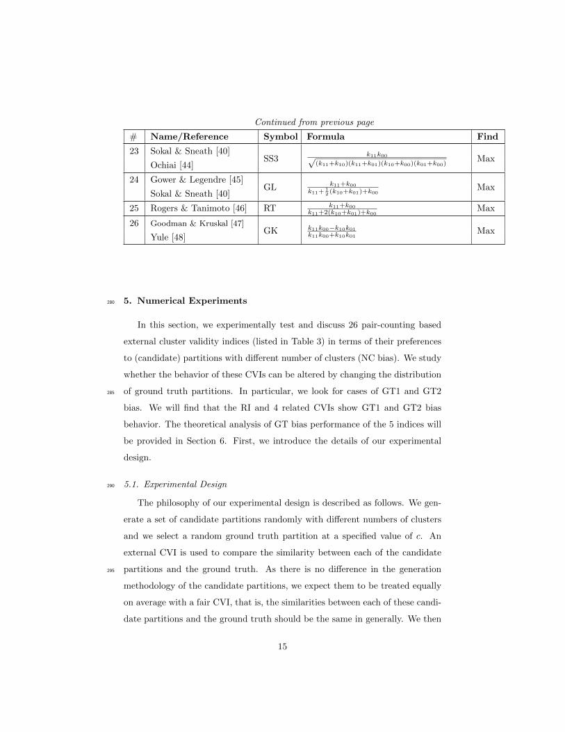
NCinc bias, and FM and JI suffered from NCdec bias. However, it was men-
tioned in this work that “... the bias with the Rand index would be to select
a solution with a larger number of clusters. The only exception occurred when165
two clusters were hypothesized to be present in the data. In this case, the bias
was reversed.” This empirical observation can be related our work. However,
there was no analysis or further discussion about this reversed bias behavior of
RI except this isolated observation. In this work, we provide a comprehensive
empirical and theoretical study of this kind of changeable bias behavior due to170
the distribution of the ground truth.
8
3. Notation and Definitions
In this section, we first introduce the notations used in this work. Then we
provide the definitions about the different bias behavior of the external CVIs,
i.e., NC bias, GT bias which further has two subtypes, i.e., GT1 bias and GT2175
bias.
3.1. Notation
Let D be a set of N objects {o1, . . . , oN}. A convenient way to represent a
crisp c − partition of D is with a set of (cN) values {uik} arrayed as a c × N
matrix U = [uik]. Element uik is the membership of ok in cluster i. We denote
the set of all possible c-partitions of D as:
MhcN = {U ∈ RcN |∀i, k, uik ∈ {0, 1};∀k,c∑i=1
uik = 1;∀i,N∑k=1
uik > 0} (1)
The cardinality (or size) of cluster i is∑Nk=1 uik = ni. When all of the ni
are equal to N/c, we say that U is balanced.
3.2. Definitions180
This section contains definitions for the types of bias exerted on external
CVIs by their functional forms (NC bias) and the distribution of the ground
truth partition (GT bias). We will call the influence of the number of clusters
in ground truth partition, UGT , Type 1 or GT1 bias, and the influence of the
size distribution of the subsets in UGT Type 2, or GT2 bias.185
Definition 1. Let UGT ∈ MhrN be any crisp ground truth partition with r
subsets, where 2 ≤ r ≤ N . Let CP = {V1, . . . , Vm}, where Vi ∈MhciN , be a set
of candidate partitions with different numbers of clusters, where 2 ≤ ci ≤ N .
We compare UGT with each Vi ∈ CP using an external Cluster Validity Index
(CVI) and choose the one that is the best match to UGT . There are two types190
of external CVIs: max-optimal (larger value is better) similarity measures such
as Rand’s index (RI); and min-optimal (smaller value is better) dissimilarity
measures such as the Mirkin metric (refer to Table 3).
9
We say an external CVI has NC bias if it shows bias behavior with respect to
the number of clusters in Vi when comparing Vi ∈ CP to the ground truth195
UGT . There are three types of NC bias status defined in this work based on our
numerical experiments 1
1. if a max-optimal (min-optimal) CVI tends to assign higher (smaller) scores
to the partition Vi ∈ CP with larger ci, then we say this CVI has NCinc
(NC increase) bias;200
2. if a max-optimal (min-optimal) CVI tends to assign smaller (higher) scores
to the partition Vi ∈ CP with larger values of ci, then we say this CVI
has NCdec (NC decrease) bias;
3. if a CVI tends to be indifferent to the values of ci for the partitions Vi ∈
CP , we say that this CVI has no NC bias. In this case, we will call the205
lack of bias NCflat.
For example, the RI shows NCinc bias in Figure 4b; JI shows NCdec bias
in Figure 4c; RI shows NCflat bias in Figure 4a and ARI shows NCflat bias
in Figure 4e. Next, we define ground truth bias (GT bias), which occurs if the
use of a different ground truth partition alters the NC bias status of an external210
CVI.
Definition 2. Let Q and Q′ denote the NC bias status of an external CVI,
with respect to two ground truth partitions, UGT and U ′GT respectively, so
Q,Q′ ∈ {NCinc,NCdec,NCflat}. If Q 6= Q′, then this external CVI has ground
truth bias (GT bias).215
For example, given two ground truth partitions UGT 6= U ′GT , if an external
CVI shows e.g., NCflat bias with UGT (e.g., Figure 4a), and shows, e.g., NCinc
bias with U ′GT (e.g., Figure 4b), then this CVI has GT bias. Definition 2
characterizes GT bias as an transition effect on the NC bias status of an external
CVI.220
1There could be other types of NC bias status, e.g., NC fluctuating, which are out of the
scope of this work and left to be discussed in the future work.
10
There are quite a few subcases of GT bias depending on the properties
of UGT and U ′GT relative to each other. In this article we have studied two
specific cases of GT bias, i.e., GT1 bias and GT2 bias. Generally speaking,
when an external CVI changes its bias status with respect to two ground truth
partitions UGT1 and UGT2, we have two cases: i) GT1 bias occurs when the225
subsets in these two ground truth partitions are uniformly distributed but with
different numbers of subsets; ii) GT2 bias occurs when these two ground truth
partitions have same number of subsets but with different distributions. The
formal definitions of GT1 bias and GT2 bias are described as follows.
Definition 3. Let UGT ∈MhrN be a balanced crisp ground truth partition with230
r subsets {u1, . . . , ur}, i.e., pi = |ui|N = 1
r , and U ′GT ∈ Mhr′N be a balanced
crisp ground truth partition with r′ subsets {u′1, . . . , u′r′}, i.e., p′i =|u′
i|N = 1
r′ ,
where r 6= r′. We say an external CVI has GT1 bias if the NC bias status for
UGT is different from that of U ′GT .
For example, given UGT with 2 balanced subsets, and U ′GT with 50 balanced235
subsets, then if an CVI shows e.g., NCflat bias with UGT , and NCinc bias with
U ′GT , then this CVI has GT1 bias (e.g., Figures 4a and 4b).
Definition 4. Let UGT ∈ MhrN be a crisp ground truth partition with r
subsets {u1, . . . , ur}, P = {p1, . . . , pr} = { |u1|N , . . . , |ur|
N } and p2 = p3 = . . . =
pr = 1−p1r−1 . Let U ′GT ∈ Mhr′N be another crisp ground truth partition with r′240
subsets {u′1, . . . , u′r′} and P ′ = {p′1, . . . , p′r′} = { |u′1|N , . . . ,
|u′r′ |N }, p
′2 = p′3 = . . . =
p′r′ =1−p′1r−1 , where r = r′ and p1 6= p′1. We say an external CVI has GT2 bias
if it exhibits different types of NC bias for UGT and U ′GT .
For example, given UGT ∈ Mh5N with p1 = 0.1 and U ′GT ∈ Mh5N with
p′1 = 0.9, if an external CVI shows, e.g., NCinc bias for UGT and shows e.g.,245
NCdec bias for U ′GT , then this CVI has GT2 bias (e.g., Figures 5a and 5b).
Figure 3 illustrates the relationship between NC bias and GT bias that is
contained in Definitions 1 - 4. In this Figure, CP denotes a set of crisp candidate
partitions with different numbers of clusters, and CV I denotes an external CVI.
11
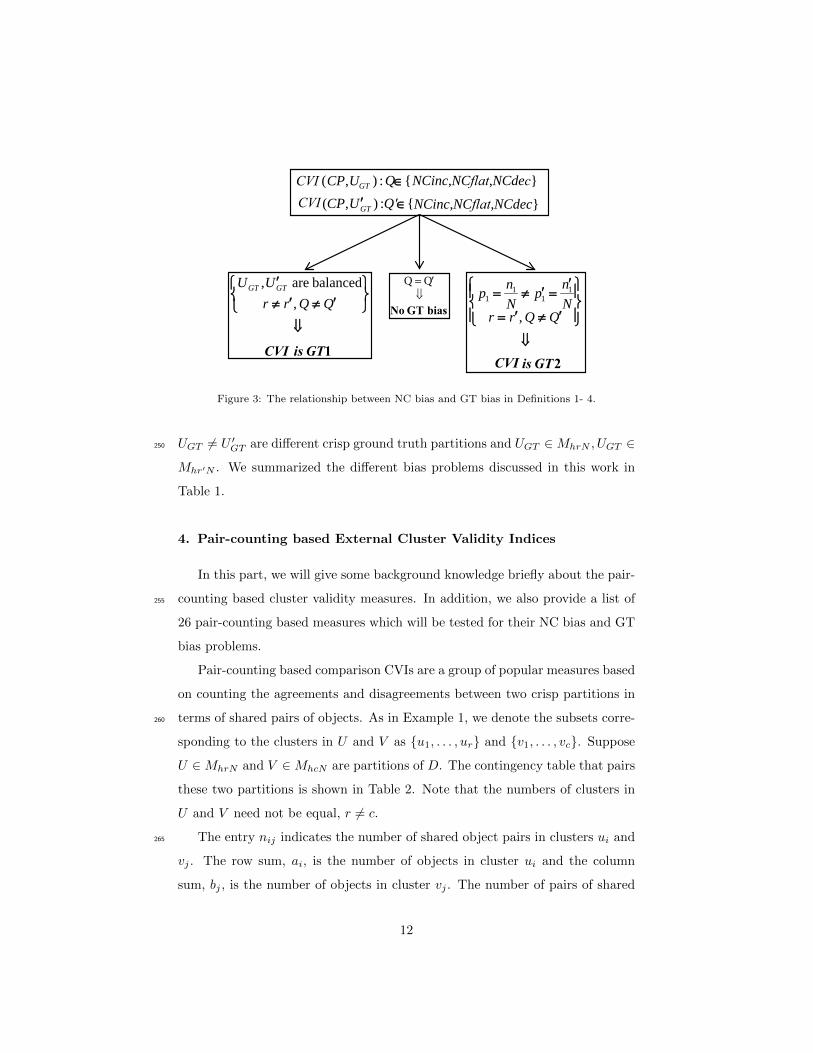
:),(,UCP
NCinc,NCflat,NCdec}UCP
GT
( ) : Q {GT
′
∈
CVICVI
Q = ′ Q ⇓
No GT bias ,balanced are ,
QQrrUU GTGT
⇓
CVI is GT1
′≠′≠
′
2
,
11
11
is GT
QQrrNnp
Nnp
CVI ⇓
′≠′=
′=′≠=
Q′∈{NCinc,NCflat,NCdec}
Figure 3: The relationship between NC bias and GT bias in Definitions 1- 4.
UGT 6= U ′GT are different crisp ground truth partitions and UGT ∈MhrN , UGT ∈250
Mhr′N . We summarized the different bias problems discussed in this work in
Table 1.
4. Pair-counting based External Cluster Validity Indices
In this part, we will give some background knowledge briefly about the pair-
counting based cluster validity measures. In addition, we also provide a list of255
26 pair-counting based measures which will be tested for their NC bias and GT
bias problems.
Pair-counting based comparison CVIs are a group of popular measures based
on counting the agreements and disagreements between two crisp partitions in
terms of shared pairs of objects. As in Example 1, we denote the subsets corre-260
sponding to the clusters in U and V as {u1, . . . , ur} and {v1, . . . , vc}. Suppose
U ∈MhrN and V ∈MhcN are partitions of D. The contingency table that pairs
these two partitions is shown in Table 2. Note that the numbers of clusters in
U and V need not be equal, r 6= c.
The entry nij indicates the number of shared object pairs in clusters ui and265
vj . The row sum, ai, is the number of objects in cluster ui and the column
sum, bj , is the number of objects in cluster vj . The number of pairs of shared
12
Table 1: Glossaries about different bias discussed in this paper.
Glossary Explanation
NC bias An external CVI shows bias behavior with respect to the
number of clusters in the compared clusterings.
NCinc bias (NC increase) One of the NC bias status. An external CVI prefers clus-
terings with larger number of clusters.
NCdec bias (NC decrease) One of the NC bias status. An external CVI prefers clus-
terings with smaller number of clusters.
NCflat bias One of the NC bias status. An external CVI has no bias
for clusterings with respect to the number of clusters.
GT bias An external CVI shows different NC bias status when vary-
ing the ground truth.
GT1 bias A subtype of GT bias. An external CVI shows different NC
bias status for two ground truths with uniform distribution
but with different numbers of subsets.
GT2 bias A subtype of GT bias. An external CVI shows different
NC bias status for two ground truths that have the same
number of subsets but with different subset distributions.
Table 2: Contingency table based on partitions U and V , nij = |ui ∩ vj |
V ∈MhcN
Cluster v1 v2 . . . vc Sums
U ∈MhrN
u1
u2
...
ur
n11 n12 . . . n1c
n21 n22 . . . n2c
......
...
nr1 nr2 . . . nrc
a1
a2...
ar
Sums b1 b2 . . . bc∑ij nij = N
objects between U and V is divided into four groups: k11, the number of pairs
that are in the same cluster in both U and V ; k00, the number of pairs that
are in different clusters in both U and V ; k10, the number of pairs that are270
in the same cluster in U but in different clusters in V ; and k01, the number
of pairs that are in different clusters in U but in the same clusters in V . And
13
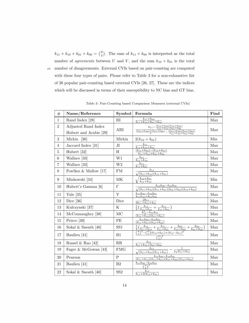
k11 + k10 + k01 + k00 =(N2
). The sum of k11 + k00 is interpreted as the total
number of agreements between U and V , and the sum k10 + k01 is the total
number of disagreements. External CVIs based on pair-counting are computed275
with these four types of pairs. Please refer to Table 3 for a non-exhaustive list
of 26 popular pair-counting based external CVIs [26, 27]. These are the indices
which will be discussed in terms of their susceptibility to NC bias and GT bias.
Table 3: Pair-Counting based Comparison Measures (external CVIs)
# Name/Reference Symbol Formula Find
1 Rand Index [28] RI k11+k00k11+k10+k01+k00
Max
2 Adjusted Rand IndexARI
k11− (k11+k10)(k11+k01)k11+k10+k01+k00
(k11+k10)+(k11+k01)2 − (k11+k10)(k11+k01)
k11+k10+k01+k00
MaxHubert and Arabie [29]
3 Mirkin [30] Mirkin 2(k10 + k01) Min
4 Jaccard Index [31] JI k11k11+k10+k01
Max
5 Hubert [32] H (k11+k00)−(k10+k01)k11+k10+k01+k00
Max
6 Wallace [33] W1 k11k11+k10
Max
7 Wallace [33] W2 k11k11+k01
Max
8 Fowlkes & Mallow [17] FM k11√(k11+k10)(k11+k01)
Max
9 Minkowski [34] MK√
k10+k01k11+k10
Min
10 Hubert’s Gamma [6] Γ k11k00−k10k01√(k11+k10)(k11+k01)(k01+k00)(k10+k00)
Max
11 Yule [35] Y k11k00−k10k01k11k10+k01k00
Max
12 Dice [36] Dice 2k112k11+k10+k01
Max
13 Kulczynski [37] K 12
(k11
k11+k10+ k11
k11+k01
)Max
14 McConnaughey [38] MCk211−k10k01
(k11+k10)(k11+k01)Max
15 Peirce [39] PE k11k00−k10k01(k11+k01)(k10+k00)
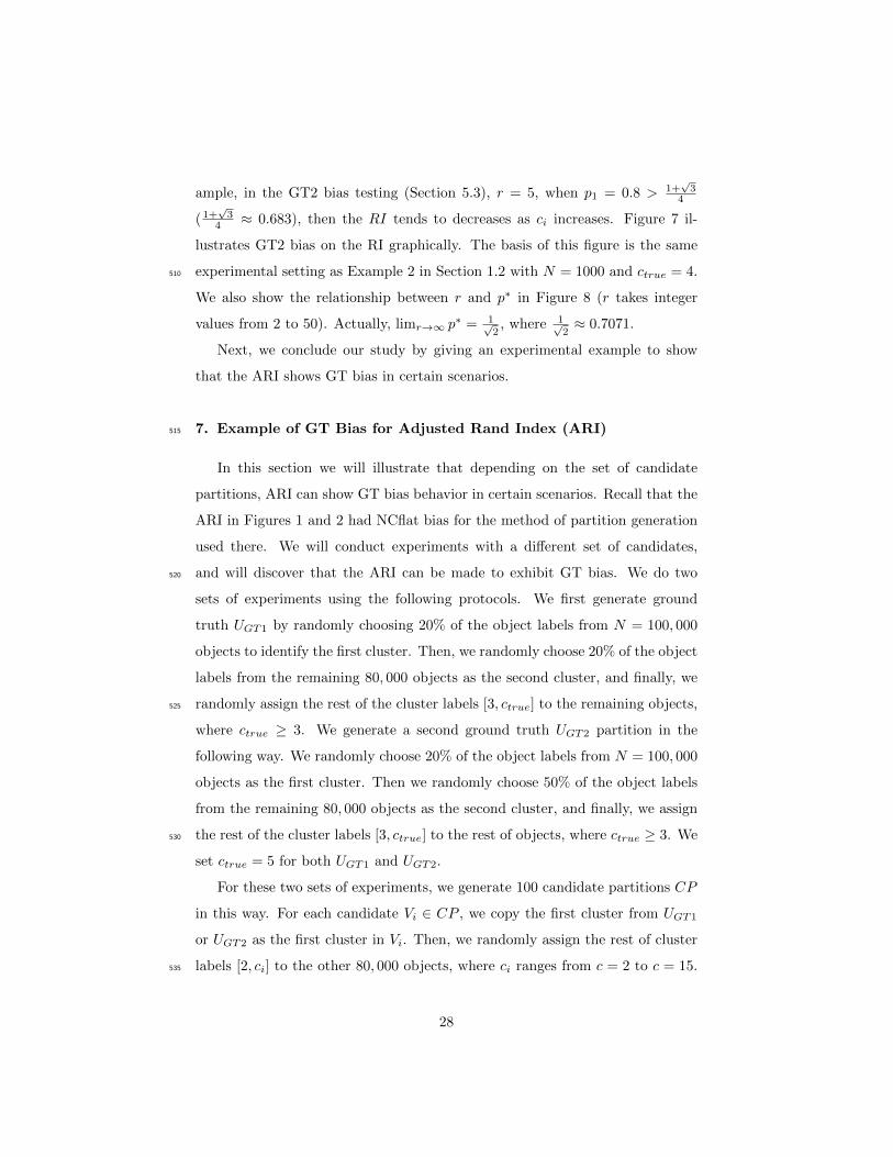
Max
16 Sokal & Sneath [40] SS1 14
(k11
k11+k10+ k11k11+k01
+ k00k10+k00
+ k00k01+k00
)Max
17 Baulieu [41] B1(N
2 )2−(N
2 )(k10+k01)+(k10−k01)2
(N2 )
2 Max
18 Russel & Rao [42] RR k11k11+k10+k01+k00
Max
19 Fager & McGowan [43] FMG k11√(k11+k10)(k11+k01)
− 12√k11+k10
Max
20 Pearson P k11k00−k10k01(k11+k10)(k11+k01)(k01+k00)(k10+k00)
Max
21 Baulieu [41] B2 k11k00−k10k01(N
2 )2 Max
22 Sokal & Sneath [40] SS2 k11k11+2(k10+k01)
Max
14
Continued from previous page
# Name/Reference Symbol Formula Find
23 Sokal & Sneath [40]SS3
k11k00√(k11+k10)(k11+k01)(k10+k00)(k01+k00)
MaxOchiai [44]
24 Gower & Legendre [45]GL k11+k00
k11+12 (k10+k01)+k00
MaxSokal & Sneath [40]
25 Rogers & Tanimoto [46] RT k11+k00k11+2(k10+k01)+k00
Max
26 Goodman & Kruskal [47]GK k11k00−k10k01
k11k00+k10k01Max
Yule [48]
5. Numerical Experiments280
In this section, we experimentally test and discuss 26 pair-counting based
external cluster validity indices (listed in Table 3) in terms of their preferences
to (candidate) partitions with different number of clusters (NC bias). We study
whether the behavior of these CVIs can be altered by changing the distribution
of ground truth partitions. In particular, we look for cases of GT1 and GT2285
bias. We will find that the RI and 4 related CVIs show GT1 and GT2 bias
behavior. The theoretical analysis of GT bias performance of the 5 indices will
be provided in Section 6. First, we introduce the details of our experimental
design.
5.1. Experimental Design290
The philosophy of our experimental design is described as follows. We gen-
erate a set of candidate partitions randomly with different numbers of clusters
and we select a random ground truth partition at a specified value of c. An
external CVI is used to compare the similarity between each of the candidate
partitions and the ground truth. As there is no difference in the generation295
methodology of the candidate partitions, we expect them to be treated equally
on average with a fair CVI, that is, the similarities between each of these candi-
date partitions and the ground truth should be the same in generally. We then
15
make a graph, taking the number of clusters of the candidate partitions as the
x axis, and the values of the external CVI between the ground truth and the300
partition with the specific number of clusters as the y axis. For a fair external
CVI, we expect this graph to be (more or less) flat.
If the line tends to go up as the number of clusters increases, then this CVI
(e.g., similarity measure) shows NCinc bias; if the line tends to go down as
the number of clusters increases, then this CVI (e.g., similarity measure) shows305
NCdec bias; if the line tends to be flat as the number of clusters increases, then
this CVI (e.g., similarity measure) shows NCflat bias, i.e., no bias.
First we test and discuss the performance of the CVIs with respect to their
NC bias. CVIs that show NCflat behavior are set aside. The remaining CVIs
are then tested to see if their NC bias behavior will be influenced or changed310
by a change in the ground truth (compared with the same set of candidate
partitions), i.e., will we see GT bias? For example, an external CVI may show
NCinc bias with one ground truth partition and show NCdec bias with another
ground truth partition; or, it may show NCflat bias with one ground truth
partition and show NCinc bias with a different ground truth partition.315
The distribution of the ground truth partition can be varied in different
ways. In this work, we consider two important factors with respect to the
ground truth: 1) the number of subsets in the ground truth (related to GT1
bias); and 2) the distribution of subsets in the ground truth (related to GT2
bias). We designed two sets of experiments for testing the GT1 and GT2 bias320
of the 26 pair-counting based external CVIs. More details are as follows.
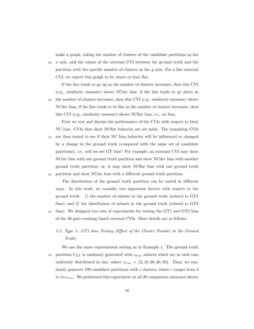
5.2. Type 1: GT1 bias Testing (Effect of the Cluster Number in the Ground
Truth)
We use the same experimental setting as in Example 1. The ground truth
partition UGT is randomly generated with ctrue subsets which are in each case325
uniformly distributed in size, where ctrue = {2, 10, 20, 30, 50}. Then, we ran-
domly generate 100 candidate partitions with c clusters, where c ranges from 2
to 3∗ctrue. We performed this experiment on all 26 comparison measures shown
16
2 3 4 5 6
Ave
rage
Val
ues
of In
dex
0
0.1
0.2
0.3
0.4
0.5
RI"
# Clusters in Candidate Partitions
NCflat
(a) RI with random UGT ∈ Mh2N , i.e.,
ctrue = 2.
20 40 60 80 100 120 140
Ave
rage
Val
ues
of In
dex
0
0.2
0.4
0.6
0.8RI"
# Clusters in Candidate Partitions
NCinc
(b) RI with random UGT ∈Mh50N , i.e.,
ctrue = 50.
⇒GT1 bias
2 3 4 5 6
Ave
rage
Val
ues
of In
dex
0
0.05
0.1
0.15
0.2
0.25
0.3 Jaccard"
# Clusters in Candidate Partitions
NCdec
(c) Jaccard with random UGT ∈Mh2N ,
i.e., ctrue = 2.
20 40 60 80 100 120 140
Ave
rage
Val
ues
of In
dex
0
0.005
0.01
0.015
Jaccard"
# Clusters in Candidate Partitions
NCdec
(d) Jaccard with random UGT ∈
Mh50N , i.e., ctrue = 50.
# Clusters Candidate Partitions2 3 4 5 6
Ave
rage
Val
ues
of In
dex
#10-3
0
2
4
6
8
10ARI"
NCflat
(e) ARI with random UGT ∈Mh2N , i.e.,
ctrue = 2.
# Clusters Candidate Partitions20 40 60 80 100 120 140
Ave
rage
Val
ues
of In
dex
#10-3
0
2
4
6
8
10ARI"
NCflat
(f) ARI with random UGT ∈ Mh50N ,
i.e., ctrue = 50.
Figure 4: 100 trial average values of the RI, JI and ARI external CVIs with variable ground
truth resulting in GT1 bias, ctrue = 2, 50.
in Table 3, but due to limited space, we focus our discussion on the results from
three representative measures, the RI, JI and ARI (indices #1,#2, and #4 in330
17
Table 3) with ctrue = 2, 50 (Figure 4). The complete results of the numeri-
cal experiments discussed in this section can be found in the supplementary
document 2.
When ctrue = 2, the RI trend is flat, that is, it has NCflat bias. But when
ctrue = 50, the RI favors solutions with larger number of clusters, i.e., it shows335
NCinc bias with ctrue = 50. Thus, the number of clusters in the random ground
truth partition UGT does influence the NC bias behavior of the RI. According to
definition 3, this indicates that RI has GT1 bias. Comparing Figures 4c and 4d
shows that the Jaccard index does not seem to suffer from GT bias due to the
number of subsets in UGT . These two figures show that the JI exhibits NCdec340
bias, decreasing monotonically as c increases from 2 to 6 (Figure 4c) or 2 to 150
(Figure 4d). Figures 4e and 4f show that the ARI is not monotonic for either
value of c, and is not affected by the number of clusters in UGT . Thus, ARI has
NCflat bias. We remark that these observed bias behavior of the tested external
CVIs are based on these experimental settings.345
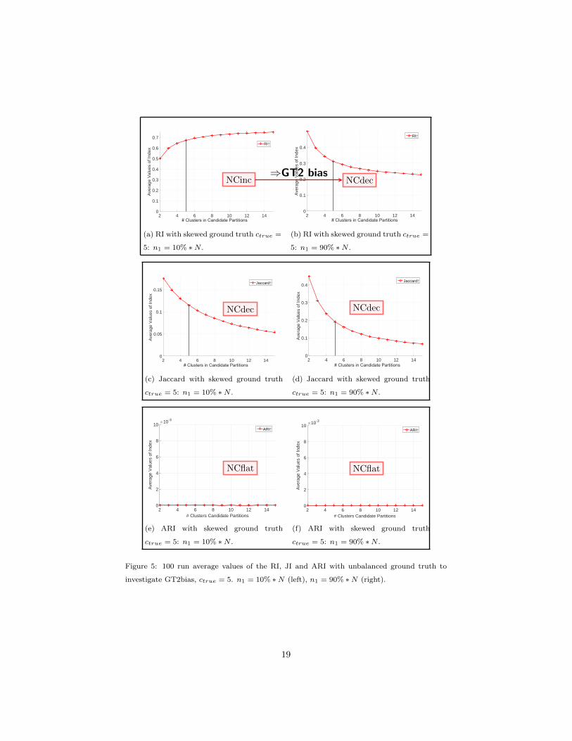
5.3. Type 2: GT2 bias Testing (Effect of the Distirbution of Clusters in Ground
Truth)
We use an experimental setup similar to that in Example 2. We generate
a ground truth by randomly assigning 10%, 20%, . . . , 90% of the objects to the
first cluster, and then randomly assigning the remaining cluster labels to the350
rest of the data objects. Here ctrue = 5 is discussed. Figure 5 shows the results
for the RI, JI and ARI with the size of the first cluster either n1 = 0.1 ∗ N or
n1 = 0.9 ∗N .
Figures 5a and 5b show that the RI suffers from GT2 bias according to
definition 4. It is monotone increasing with n1 = 10, 000 (NCinc bias), but355
monotone decreasing with n1 = 90, 000 (NCdec bias). Note that the graphs
in Figures 5a and 5b are reflections of each other about the horizontal axis at
0.5. The Jaccard index in Figures 5c and 5d exhibits the same NC bias status
2The supplementary document is available at https://sites.google.com/site/yldatascience/
18
2 4 6 8 10 12 14
Ave
rage
Val
ues
of In
dex
0
0.1
0.2
0.3
0.4
0.5
0.6
0.7RI"
# Clusters in Candidate Partitions
NCinc
(a) RI with skewed ground truth ctrue =
5: n1 = 10% ∗N .
2 4 6 8 10 12 14
Ave
rage
Val
ues
of In
dex
0
0.1
0.2
0.3
0.4
RI"
# Clusters in Candidate Partitions
NCdec
(b) RI with skewed ground truth ctrue =
5: n1 = 90% ∗N .
⇒GT2 bias
2 4 6 8 10 12 14
Ave
rage
Val
ues
of In
dex
0
0.05
0.1
0.15
Jaccard"
# Clusters in Candidate Partitions
NCdec
(c) Jaccard with skewed ground truth
ctrue = 5: n1 = 10% ∗N .
2 4 6 8 10 12 14
Ave
rage
Val
ues
of In
dex
0
0.1
0.2
0.3
0.4Jaccard"
# Clusters in Candidate Partitions
NCdec
(d) Jaccard with skewed ground truth
ctrue = 5: n1 = 90% ∗N .
# Clusters Candidate Partitions2 4 6 8 10 12 14
Ave
rage
Val
ues
of In
dex
#10-3
0
2
4
6
8
10ARI"
NCflat
(e) ARI with skewed ground truth
ctrue = 5: n1 = 10% ∗N .
# Clusters Candidate Partitions2 4 6 8 10 12 14
Ave
rage
Val
ues
of In
dex
#10-3
0
2
4
6
8
10ARI"
NCflat
(f) ARI with skewed ground truth
ctrue = 5: n1 = 90% ∗N .
Figure 5: 100 run average values of the RI, JI and ARI with unbalanced ground truth to
investigate GT2bias, ctrue = 5. n1 = 10% ∗N (left), n1 = 90% ∗N (right).
19
as it did in Figures 4c and 4d. Specifically, JI decreases monotonically with c,
so it still has NCdec bias, but it does not seem to be affected by GT2 bias.360
The ARI in Figures 5e and 5f does not show any influence due to GT2 bias.
It has NCflat bias under these two sets of experimental settings. So, from our
empirical results, ARI would appear to be preferable to the RI and the JI in this
setting. To summarize, these examples illustrate that the RI can suffer from
GT1 bias and GT2 bias; that JI can suffer from NCdec bias but not GT1 bias365
nor GT2 bias; and that ARI does not suffer from NC bias or GT bias, under
the experimental setup we have used here.
5.4. Summary for All 26 Comparison Measures
The overall results of similar experiments for all 26 indices (refer to supple-
mentary document) in Table 3 led to the conclusion that 5 of the 26 external370
CVIs suffer from GT1 bias and GT2 bias for these experimental settings. These
measures are Rand Index (RI) and
Hubert [32] : H(U, V ) = 2RI − 1 (2)
Gower and Legendre [45] : GL(U, V ) =2
1 + 1/RI(3)
Rogers and Tanimoto [46] : RT (U, V ) =1
2/RI − 1(4)
Mirkin [30] : Mirkin(U, V ) = N(N − 1)(1−RI) (5)
Please note that the external CVIs in equations 2, 3, 4 and 5 are all functions
of the RI. This observation forms the basis for our analysis in the next section.
6. Bias Due to Ground Truth for the Rand Index375
In this section, we provide a theoretical analysis for the GT bias, GT1 bias
and GT2 bias for the Rand Index. More specifically, we will analyze the under-
lying reason for the GT bias of RI, based on its relationship with the quadratic
entropy (Equation 8). Then, based on the relationship between RI and the
20
quadratic entropy, we will discuss theoretically about when RI shows GT bias,380
GT1 bias and GT2 bias, according to the distribution of the ground truth and
the number of subsets in the ground truth.
6.1. Quadratic Entropy and Rand Index
The Havrda-Charvat entropy [49] (Equation 6) is a generalization of the
Shannon entropy (Equation 7). The quadratic entropy (Equation 8) is the385
Havrda-Charvat generalized entropy with β = 2.
6.1.1. Havrda-Charvat Generalized Entropy
The Havrda-Charvat generalized entropy for a crisp partition U with r clus-
ters U = {u1, . . . , ur} is
Hβ(U) =1
1− 21−β(1−
r∑i=1
(|ui|N
)β) (6)
where β is any real number > 0 and β 6= 1. Since H is a continuous function of
β, when β = 1
H1(U) = −r∑i=1
|ui|N
log|ui|N
(7)
which is the Shannon entropy HS(U). When β = 2 we have quadratic entropy
H2(U) = 2(1−r∑i=1
(|ui|N
)2) (8)
It can be shown that in the case of statistically independent random variables
U and V
Hβ(U, V ) = Hβ(U) +Hβ(V )− (1− 21−β)Hβ(U)Hβ(V ) (9)
When β = 2, Equation 9 becomes
H2(U, V ) = H2(U) +H2(V )− 1
2H2(U)H2(V ) (10)
In [50], Meila showed that the Variation of Information (VI) is a metric by
expressing it as a function of Shannon’s entropy. Consider a crisp partition V
21
with c subsets V = {v1, . . . , vc}, then
V I(U, V ) = HS(U |V ) +HS(V |U) (11)
= 2HS(U, V )−HS(U)−HS(V )
The VI is not one of the 26 indices in Table 3, but this information-theoretic
CVI can be computed based on the contingency table, and it will help us analyze
the GT bias of the 5 external CVIs discussed in Section 5.4.390
Simovici [51] showed that replacing Shannon’s entropy in Equation 11 by
the generalized entropy at Equation 6 still yielded a metric,
V Iβ(U, V ) = Hβ(U |V ) +Hβ(V |U) (12)
= 2Hβ(U, V )−Hβ(U)−Hβ(V ) (13)
For β = 2, this becomes
V I2(U, V ) = 2H2(U, V )−H2(U)−H2(V ) (14)
Based on the above introduced concepts, we next introduce how to derive
the relationship between RI and the quadratic entropy (i.e., Havrda-Charvat
generalized entropy with β = 2). This relationship will help us explain why RI
shows GT bias.
6.1.2. Quadratic Entropy vs. Rand Index395
Let U and V be two crisp partitions of N samples with r clusters and c
clusters respectively. Then the relationship between V I2(U, V ) and RI(U, V )
can be derived as follows [51].
First, based on Equations 13 and 6, we have V Iβ(U, V ) as
V Iβ(U, V ) = 2Hβ(U, V )−Hβ(U)−Hβ(V ) (15)
=2
1− 21−β(1−
r∑i=1
c∑j=1
(|ui ∩ vj |N
)β)− 1
1− 21−β(1−
r∑i=1
|ui|N
)β − 1
1− 21−β(1−
c∑j=1
(|vj |N
)β)
=1
1− 21−β(2(1−
r∑i=1
c∑j=1
(|ui ∩ vj |N
)β)− (1−r∑i=1
(|ui|N
)β)− (1−c∑j=1
(|vj |N
)β))
=1
Nβ(1− 21−β)(
r∑i=1
(|ui|)β +
c∑j=1
(|vj |)β − 2
r∑i=1
c∑j=1
(|ui ∩ vj |)β)
22
Now setting β = 2, we get
V I2(U, V ) =2
N2(
r∑i=1
(|ui|)2 +
c∑j=1
(|vj |)2 − 2
r∑i=1
c∑j=1
(|ui ∩ vj |)2)
=2
N2(2k10 + 2k01)
=2
N(N − 1)(1−RI(U, V )) (16)
Equation 16 shows that V I2 and RI are inversely related. Thus, by analyzing400
the bias behavior of V I2, it will be easy to understand the behavior of RI. Next,
we will analyze the GT bias behavior of V I2 based on the concept of quadratic
entropy.
6.2. GT bias of RI
In this section, we will first discuss the general case of GT bias for RI by405
providing a series of theoretical statements for helping understand why RI shows
GT bias, and when RI shows GT bias. Then, we will discuss two specific cases,
i.e., GT1 bias and GT2 bias for RI and provide related theoretical statements
which will explain when RI shows GT1 bias and GT2 bias. The related proofs
are provided in Appendix A.410
6.2.1. General Case of GT bias
We introduce Lemma 1 to build the foundation for analyzing the GT bias
of V I2, then RI.
Lemma 1. Given U ∈ MhrN and V ∈ MhcN , two statistically independent
crisp partitions of N data objects, we have
V I2(U, V ) = H2(U) + (1−H2(U))H2(V ) (17)
Next, we introduce an important theorem in this paper that demonstrates
why RI shows GT bias and when it shows GT bias by judging the relationship415
between the quadratic entropy of ground truth UGT , H2(UGT ) and 1.
23
Theorem 1. Let UGT ∈MhrN be a ground truth partition with r subsets, and
let CP = {V1, . . . , Vm} be a set of candidate partitions with different numbers of
clusters, where Vi ∈MhciN contains ci clusters which are uniformly distributed
(balanced), 2 ≤ ci ≤ N . Assuming UGT and Vi ∈ CP are statistically indepen-420
dent, then RI suffers from GT bias. In addition, according to the relationship
between H2(UGT ) and 1, we have:
1. if H2(UGT ) < 1, RI suffers from NCdec bias (i.e., RI decreases as ci
increases);
2. IfH2(UGT ) = 1, RI is unbiased, i.e., NCflat bias (i.e., RI has no preferences425
as ci increases);
3. if H2(UGT ) > 1, RI suffers from NCinc bias (i.e., RI increases as ci in-
creases).
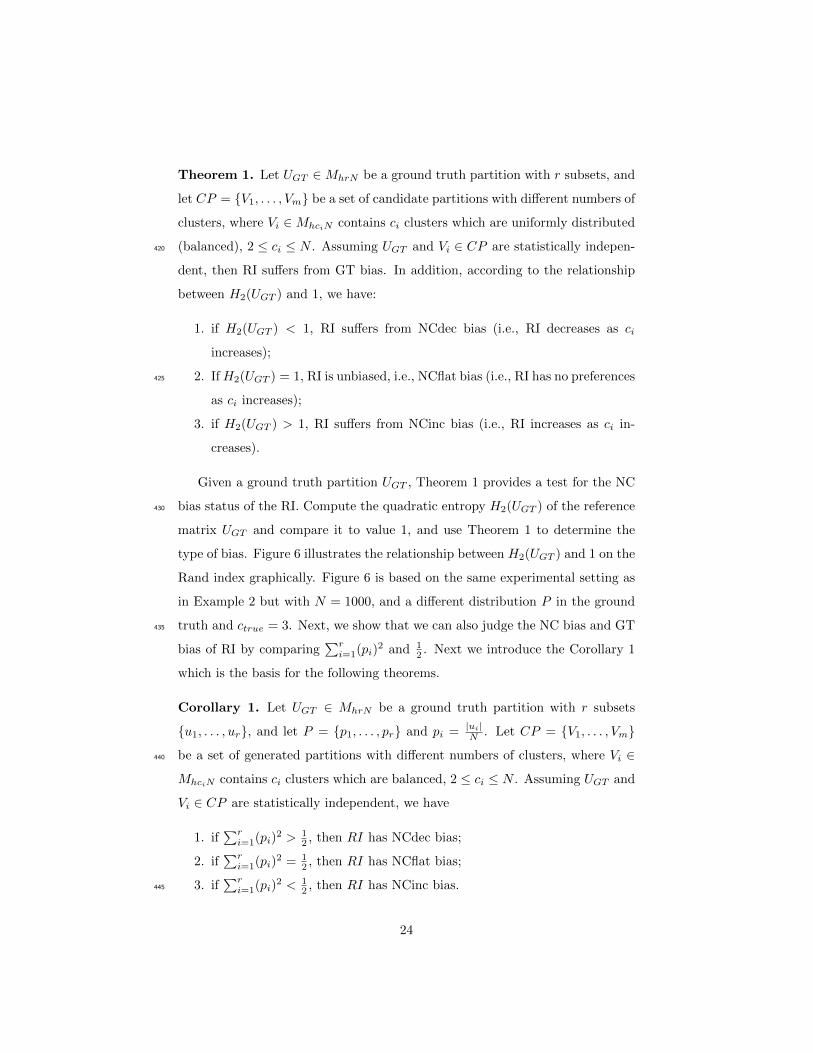
Given a ground truth partition UGT , Theorem 1 provides a test for the NC
bias status of the RI. Compute the quadratic entropy H2(UGT ) of the reference430
matrix UGT and compare it to value 1, and use Theorem 1 to determine the
type of bias. Figure 6 illustrates the relationship between H2(UGT ) and 1 on the
Rand index graphically. Figure 6 is based on the same experimental setting as
in Example 2 but with N = 1000, and a different distribution P in the ground
truth and ctrue = 3. Next, we show that we can also judge the NC bias and GT435
bias of RI by comparing∑ri=1(pi)
2 and 12 . Next we introduce the Corollary 1
which is the basis for the following theorems.
Corollary 1. Let UGT ∈ MhrN be a ground truth partition with r subsets
{u1, . . . , ur}, and let P = {p1, . . . , pr} and pi = |ui|N . Let CP = {V1, . . . , Vm}
be a set of generated partitions with different numbers of clusters, where Vi ∈440
MhciN contains ci clusters which are balanced, 2 ≤ ci ≤ N . Assuming UGT and
Vi ∈ CP are statistically independent, we have
1. if∑ri=1(pi)
2 > 12 , then RI has NCdec bias;
2. if∑ri=1(pi)
2 = 12 , then RI has NCflat bias;
3. if∑ri=1(pi)
2 < 12 , then RI has NCinc bias.445
24
2 3 4 5 6 7 8 9
# Clusters in Candidate Partitions
0
0.05
0.1
0.15
0.2
0.25
0.3
0.35
0.4
0.45
0.5
Aver
age
RI V
alue
s
600:50:350 (H 2(U
GT)=1.03, NC
inc)
600:100:300 (H2(U
GT)=1.08, NC
inc)
600:150:250 (H2(U
GT)=1.11, NC
inc)
600:200:200 (H2(U
GT)=1.12, NC
inc)
700:50:250 (H 2(U
GT)=0.89, NC
dec)
700:100:200 (H2(U
GT)=0.92, NC
dec)
700:150:150 (H2(U
GT)=0.93, NC
dec)
2000:100:20 (H2(U
GT)=0.22, NC
dec)
(ctrue)
Figure 6: 100 trial average RI values with ci ranging from 2 to 9 for ctrue = 3. n1 : n2 : n3
indicates the sizes of the three clusters and the corresponding H2(UGT ) values.
Next, we introduce another theorem which helps us understand how do the
prior probabilities {pi} and the number of subsets r in the ground truth UGT
influence the NC bias status of RI.
Theorem 2. Let UGT ∈ MhrN be a ground truth partition with r subsets
{u1, . . . , ur}, and let P = {p1, . . . , pr} and pi = |ui|N . Let P ′ = {p′1, p′2, . . . , p′r}450
denote P sorted into descending order, where p′1 ≥ p′2 . . . ≥ p′r. Let CP =
{V1, . . . , Vm} be a set of generated partitions with different numbers of clusters,
where Vi ∈MhciN contains ci clusters which are balanced, 2 ≤ ci ≤ N . Assum-
ing UGT and Vi ∈ CP are statistically independent, then RI has GT bias. In
addition, depending on P and r, we have:455
When r > 2
1. if p′1 >12 , and
if p′1(p′1 − 12 ) >
∑ri=2 p
′i(
12 − p
′i), then RI has NCdec bias;
if p′1(p′1 − 12 ) =
∑ri=2 p
′i(
12 − p
′i), then RI has NCflat bias;
if p′1(p′1 − 12 ) <
∑ri=2 p
′i(
12 − p
′i), then RI has NCinc bias.460
2. if p′1 = 12 , then RI has NCinc bias;
3. if p′1 <12 , then RI has NCinc bias.
When r = 2
25
1. if p′1 >12 , then RI has NCdec bias;
2. if p′1 = 12 , then RI has NCflat bias.465
Theorem 2 tells us how the ground truth distribution P ′ and the number
of clusters r of UGT affect the Rand index and helps us judge the NC bias
status based on P ′ and r. For example, if r > 2, p′1 >12 and p′1(p′1 − 1
2 ) >∑ri=2 p
′i(
12 − p′i), then RI has NCdec bias (e.g., r = 3, p′1 = 2
3 , p′2 = 1
4 and
p′3 = 112 ). If r = 2 and p′1 = 1
2 , then RI has NCflat bias. Thus RI has GT bias.470
The above discussion and theoretical analysis are in a more general sense.
Next, we discuss GT1 bias and GT2 bias of the RI, which are two specific types
of GT bias with certain conditions imposed on the ground truth. This will also
help explain and judge the NC bias behavior of the indices in the empirical test
shown Section 5.475
6.2.2. GT1 bias and GT2 bias
First, we start by introducing a theorem for GT1 bias of RI.
Theorem 3. Let UGT ∈ MhrN be a crisp ground truth partition with r bal-
anced subsets {u1, . . . , ur}, i.e., pi = |ui|N = 1
r . Let CP = {V1, . . . , Vm} be a set
of generated partitions with different numbers of clusters, where Vi ∈ MhciN480
contains ci clusters which are balanced, 2 ≤ ci ≤ N . Assuming UGT and
Vi ∈ CP are statistically independent, then RI suffers from GT1 bias. More
specifically,
1. if r = 2, then RI has NCflat bias;
2. if r > 2, then RI has NCinc bias.485
Theorem 3 provides an explanation of how GT1 bias influences RI. For
example, it is easier to understand the behavior of RI shown in the GT1 bias
testing in Section 5.2 (Figures 4a and 4b). Next, we introduce a theorem for
the GT2 bias of RI.
Theorem 4. Let UGT ∈ MhrN be a ground truth partition with r subsets490
{u1, . . . , ur}. Assume the first cluster u1 in the ground truth has variable sizes,
26
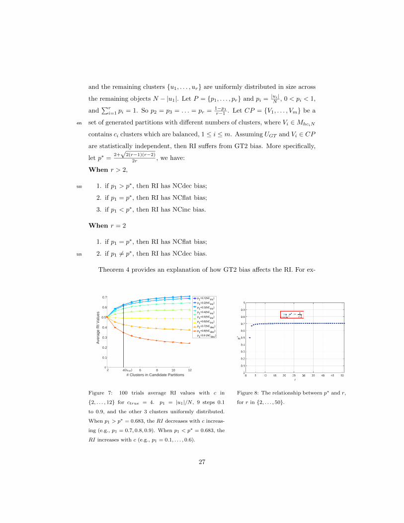
and the remaining clusters {u1, . . . , ur} are uniformly distributed in size across
the remaining objects N − |u1|. Let P = {p1, . . . , pr} and pi = |ui|N , 0 < pi < 1,
and∑ri=1 pi = 1. So p2 = p3 = . . . = pr = 1−p1
r−1 . Let CP = {V1, . . . , Vm} be a
set of generated partitions with different numbers of clusters, where Vi ∈MhciN495
contains ci clusters which are balanced, 1 ≤ i ≤ m. Assuming UGT and Vi ∈ CP
are statistically independent, then RI suffers from GT2 bias. More specifically,
let p∗ =2+√
2(r−1)(r−2)2r , we have:
When r > 2,
1. if p1 > p∗, then RI has NCdec bias;500
2. if p1 = p∗, then RI has NCflat bias;
3. if p1 < p∗, then RI has NCinc bias.
When r = 2
1. if p1 = p∗, then RI has NCflat bias;
2. if p1 6= p∗, then RI has NCdec bias.505
Theorem 4 provides an explanation of how GT2 bias affects the RI. For ex-
2 4 10 12
# Clusters in Candidate Partitions
0
0.1
0.2
0.3
0.4
0.5
0.6
0.7
Ave
rage
RI V
alue
s
p1=0.1(NCinc)
p1=0.2(NCinc)
p1=0.3(NCinc)
p1=0.4(NCinc)
p1=0.5(NCinc)
p1=0.6(NCinc)
p1=0.7(NCdec)
p1=0.8(NCdec)
p1=0.9 (NCdec)
(ctrue) 6 8
Figure 7: 100 trials average RI values with c in
{2, . . . , 12} for ctrue = 4. p1 = |u1|/N , 9 steps 0.1
to 0.9, and the other 3 clusters uniformly distributed.
When p1 > p∗ = 0.683, the RI decreases with c increas-
ing (e.g., p1 = 0.7, 0.8, 0.9). When p1 < p∗ = 0.683, the
RI increases with c (e.g., p1 = 0.1, . . . , 0.6).
Figure 8: The relationship between p∗ and r,
for r in {2, . . . , 50}.
27
ample, in the GT2 bias testing (Section 5.3), r = 5, when p1 = 0.8 > 1+√3
4
( 1+√3
4 ≈ 0.683), then the RI tends to decreases as ci increases. Figure 7 il-
lustrates GT2 bias on the RI graphically. The basis of this figure is the same
experimental setting as Example 2 in Section 1.2 with N = 1000 and ctrue = 4.510
We also show the relationship between r and p∗ in Figure 8 (r takes integer
values from 2 to 50). Actually, limr→∞ p∗ = 1√2, where 1√
2≈ 0.7071.
Next, we conclude our study by giving an experimental example to show
that the ARI shows GT bias in certain scenarios.
7. Example of GT Bias for Adjusted Rand Index (ARI)515
In this section we will illustrate that depending on the set of candidate
partitions, ARI can show GT bias behavior in certain scenarios. Recall that the
ARI in Figures 1 and 2 had NCflat bias for the method of partition generation
used there. We will conduct experiments with a different set of candidates,
and will discover that the ARI can be made to exhibit GT bias. We do two520
sets of experiments using the following protocols. We first generate ground
truth UGT1 by randomly choosing 20% of the object labels from N = 100, 000
objects to identify the first cluster. Then, we randomly choose 20% of the object
labels from the remaining 80, 000 objects as the second cluster, and finally, we
randomly assign the rest of the cluster labels [3, ctrue] to the remaining objects,525
where ctrue ≥ 3. We generate a second ground truth UGT2 partition in the
following way. We randomly choose 20% of the object labels from N = 100, 000
objects as the first cluster. Then we randomly choose 50% of the object labels
from the remaining 80, 000 objects as the second cluster, and finally, we assign
the rest of the cluster labels [3, ctrue] to the rest of objects, where ctrue ≥ 3. We530
set ctrue = 5 for both UGT1 and UGT2.
For these two sets of experiments, we generate 100 candidate partitions CP
in this way. For each candidate Vi ∈ CP , we copy the first cluster from UGT1
or UGT2 as the first cluster in Vi. Then, we randomly assign the rest of cluster
labels [2, ci] to the other 80, 000 objects, where ci ranges from c = 2 to c = 15.535
28
2 4 6 8 10 12 14
Ave
rage
Val
ues
of In
dex
0
0.05
0.1
0.15
0.2
0.25ARI"
# Clusters in Candidate Partitions
NCinc
(a) The average ARI values for UGT1
and random partitions with different
numbers of clusters.
2 4 6 8 10 12 14
Ave
rage
Val
ues
of In
dex
0
0.05
0.1
0.15
0.2
0.25ARI"
# Clusters in Candidate Partitions
NCdec
(b) The average ARI values for UGT2
and random partitions with different
numbers of clusters.
⇒GT bias
Figure 9: 100 trial average ARI values for two different ground truth and set of candidates
with different numbers of clusters.
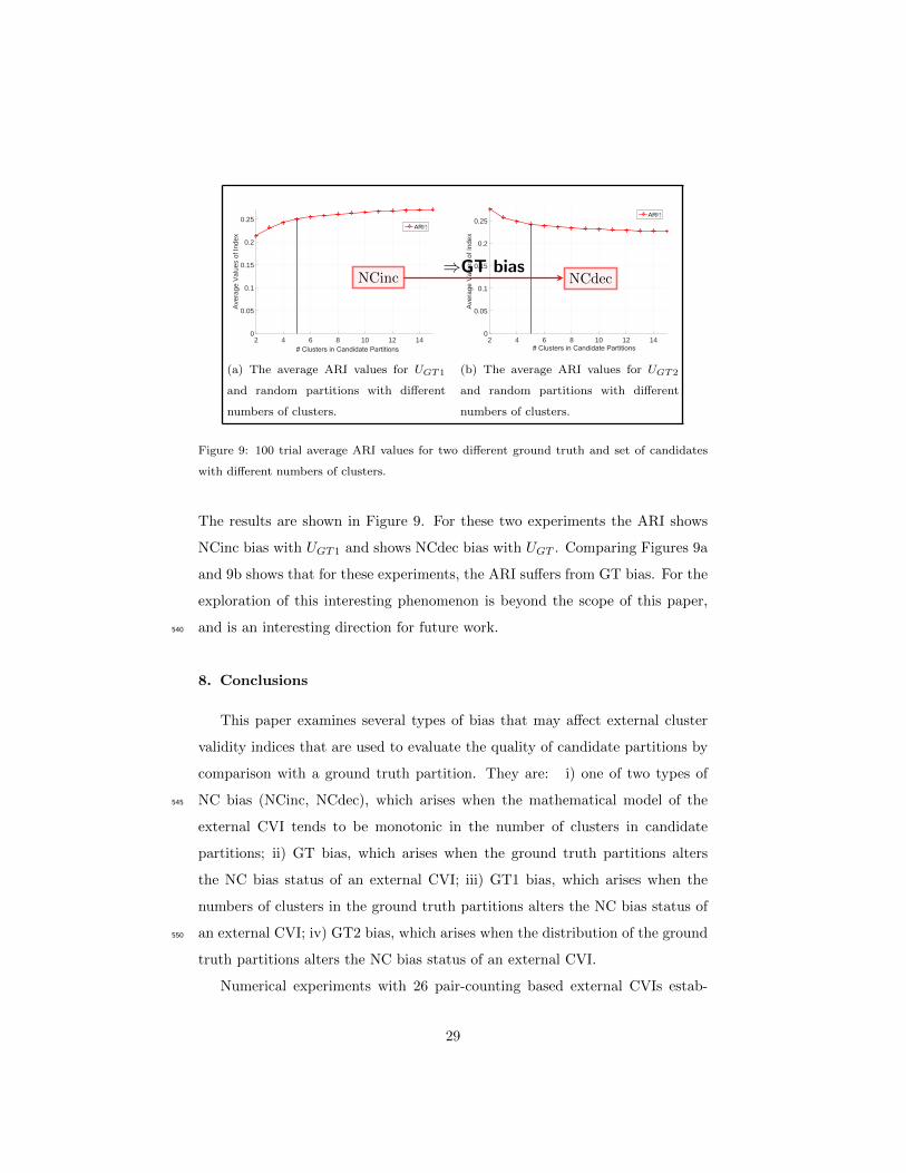
The results are shown in Figure 9. For these two experiments the ARI shows
NCinc bias with UGT1 and shows NCdec bias with UGT . Comparing Figures 9a
and 9b shows that for these experiments, the ARI suffers from GT bias. For the
exploration of this interesting phenomenon is beyond the scope of this paper,
and is an interesting direction for future work.540
8. Conclusions
This paper examines several types of bias that may affect external cluster
validity indices that are used to evaluate the quality of candidate partitions by
comparison with a ground truth partition. They are: i) one of two types of
NC bias (NCinc, NCdec), which arises when the mathematical model of the545
external CVI tends to be monotonic in the number of clusters in candidate
partitions; ii) GT bias, which arises when the ground truth partitions alters
the NC bias status of an external CVI; iii) GT1 bias, which arises when the
numbers of clusters in the ground truth partitions alters the NC bias status of
an external CVI; iv) GT2 bias, which arises when the distribution of the ground550
truth partitions alters the NC bias status of an external CVI.
Numerical experiments with 26 pair-counting based external CVIs estab-
29
lished that for the method described in the examples, 5 of the 26 suffer from
GT1bias and/or GT2bias, viz., the indices due to Rand (#1), Mirkin (#3),
Hubert (#5), Gower and Legendre (#24) and Rogers and Tanimoto (#25), the555
numbers referring to rows in Table 3. Actually, the 4 indices, Mirkin (#3),
Hubert (#5), Gower and Legendre (#24) and Rogers and Tanimoto (#25), are
all functions of RI. We point out that the observed bias behavior (NC bias, GT1
bias and GT2 bias) of the tested 26 indices was based on a particular way to
obtain candidate partitions. In our experiments the “clustering algorithm” used560
to generate the CPs was random draws from MhciN . It is entirely possible that
sets of CPs secured, for example, by running clustering clustering algorithms
on a dataset will NOT exhibit the same bias tendencies. This is just another
difficulty of external cluster validity indices, as was illustrated by the fact that
we could change the bias status of the ARI by changing the method of securing565
the candidate. The major point of this work is to draw attention to the fact
that there can be a GT bias problem for external CVIs.
We then formulated an explanation for both types of GT bias with Rand
Index based on the the Havrda-Charvat quadratic entropy. Our theory ex-
plained how RI’s NC bias behavior is influenced by the distribution of the570
ground truth partition and also the number of clusters in the ground truth.
Our major results in Theorem 1, which provides a computable test that pre-
dicts the NC bias behavior of the Rand Index, and hence, all external CVIs
related to it. Rand Index has been one of the most popular external CVIs due
to its simple, natural interpretation and has recently been applied in many re-575
search work [10, 11, 12, 14, 15, 16]. Thus, the identified GT bias behavior for
RI with correponding explaination could be helpful for users who apply RI in
their work. Finally, we gave an experimental example showing that the ARI
can suffer from GT bias in certain scenarios.
We believe this to be the first systematic study of the effects of ground580
truth on the NC bias behavior of external cluster validity indices. We have
termed this GT bias. There are many other external CVIs which have not been
tested numerically or analyzed theoretically for GT bias. Our next undertaking
30
will be to study this phenomenon in the more general setting afforded by non
pair-counting based external CVIs.585
Appendix A. Proofs
Proof of Lemma 1. As U and V are statistically independent, we can sub-
stitute Equation 10 into Equation 14, obtaining
V I2(U, V ) = 2H2(U, V )−H2(U)−H2(V )
= 2(H2(U) +H2(V )− 1
2H2(U)H2(V )
)−H2(U)−H2(V )
= H2(U) + (1−H2(U))H2(V ) (A.1)
Proof of Theorem 1. According to lemma 1,
V I2(UGT , V ) = H2(UGT ) + (1−H2(UGT ))H2(V ) = a+ bx (A.2)
where a = H2(UGT ) and b = (1−H2(UGT )) = (1− a) and x = H2(V ). As any
Vi ∈ CP is uniformly distributed (balanced), then H2(Vi) = 2(1 −∑cii=1( 1
ci)2)
(refer to equation 8) and H2(Vi) increases as ci increases. It is clear from
equation (A.2) that for fixed UGT , V I2 can be regarded as a straight line with590
y intercept a = H2(UGT ) and slope b = 1 −H2(UGT ) = (1 − a), so the rate of
growth (or decrease, or neither (flat)) of V I2 depends on b. In other words, V I2
could be increasing, decreasing or flat as ci increases. More specifically, i) if
b > 0, then H2(UGT ) < 1, thus V I2 increases as x (and ci) increases; ii) if b = 1,
then H2(UGT ) = 1, thus V I2 is constant as x (and ci) increases; iii) if b < 0,595
then H2(UGT ) > 1, thus V I2 decreases as x (and ci) increases. According
to Equation 16, we know that V I2 and RI are inversely related. Thus, it is
straightforward to prove the statements.
Proof of Corollary 1. According to Theorem 1, we know that depending on
the relationship between H2(UGT ) and 1, i.e., the slope b in Equation A.2, that600
RI shows different NC bias status. As H2(UGT ) = 2(1−∑ri=1 p
2i ) (Equation 8),
then b = 1−H2(UGT ) = 1− 2(1−∑ri=1 p
2i ) = 2(
∑ri=1 p
2i − 1
2 ). Thus, we know
31
that the slope b, i.e., the relationship between H2(UGT ) and 1, depends on the
relationship between∑ri=1 p
2i and 1
2 . So, the three assertions of the corollary
follow by noting the relationship between∑ri=1 p
2i and 1
2 .605
Proof of Theorem 2. According to Corollary 1, we know that the relationship
between∑ri=1 p
2i and 1
2 influences the NC bias status of RI. It is straightforward
to see that pi and r influence the relationship between∑ri=1 p
2i and 1
2 , thus pi
and r can potentially alter the NC bias status of RI. We have
r∑i=1
(p′i)2 − 1
2=
r∑i=1
(p′i)2 − 1
2
r∑i=1
p′i = p′1(p′1 −1
2) +
r∑i=2
p′i(p′i −
1
2) (A.3)
Please note that p′1 is the biggest cluster’s density in the ground truth,
based on which we discuss and summarize the influence of pi and r on the
NC bias status of RI. We can discuss the relationship between p′1(p′1 − 12 ) and∑r
i=2 p′i(p′i− 1
2 ), which is equivalent to the relationship between∑ri=1 p
2i and 1
2 ,
for the different NC bias status.610
When r > 2: 1) if p′1 >12 , because
∑ri=1 p
′i = 1, then p′2, . . . , p
′r <
12 . Thus,
with the help of Corollary 1, we have: i) if p′1(p′1 − 12 ) >
∑ri=2 p
′i(
12 − p
′i), then∑r
i=1(p′i)2 > 1
2 , thus RI has NCdec bias; ii) if p′1(p′1− 12 ) =
∑ri=2 p
′i(
12−p
′i), then∑r
i=1(p′i)2 = 1
2 , thus RI has NCflat bias; iii) if p′1(p′1 − 12 ) <
∑ri=2 p
′i(
12 − p
′i),
then∑ri=1(p′i)
2 < 12 , thus RI has NCinc bias.615
2) if p′1 = 12 , then p′2, . . . , p
′r <
12 and
∑ri=1(p′i)
2 < 12 , thus RI has NCinc bias;
3) if p′1 <12 , then p′2, . . . , p
′r <
12 and
∑ri=1(p′i)
2 < 12 , thus RI has NCinc bias.
When r = 2: 1) if p′1 >12 , then p′1(p′1 − 1
2 ) > p′2( 12 − p
′2) and
∑ri=1(p′i)
2 > 12 ,
thus RI has NCdec bias; 2) if p′1 = 12 , then p′2 = 1
2 and∑ri=1(p′i)
2 = 12 , thus RI
has NCflat bias. Thus, the RI suffers from GT bias according to the distribution620
of ground truth P and the number of clusters r in the ground truth.
Proof of Theorem 3. Corollary 1 shows that the NC bias of the RI depends on
the relationship between∑ri=1(pi)
2 and 12 . Since pi = 1
r , then∑ri=1(pi)
2− 12 = 1
2
Then, according to Corollary 1, we have i) if r = 2, then RI has NCflat
bias; ii) if r > 2, then RI has NCinc bias. By definition 3, different values for r625
32
in UGT , i.e., r = 2 or r > 2, result in different NC bias status for the RI, thus
RI has GT1 bias.
Proof of Theorem 4. According to Corollary 1, we know that the relationship
between∑ri=1(pi)
2 and 12 determines the NC bias status of the RI. As pi = 1−p1
r−1 ,
i = 2, . . . , r, we have:
r∑i=1
p2i −1
2= p21 +
r∑i=2
p2i −1
2
=r
r − 1p21 −
2
r − 1p1 +
3− r2(r − 1)
(A.4)
Equation A.4 is quadratic in p1, and has one real positive root p∗ =2+√
2(r−1)(r−2)2r
in our case. Then:
When r > 2: i) if p1 > p∗, then∑ri=1(pi)
2 > 12 , thus RI has NCdec bias;630
ii) if p1 = p∗, then∑ri=1(pi)
2 = 12 , thus RI has NCflat bias; iii) if p1 < p∗, then∑r
i=1(pi)2 < 1
2 , thus RI has NCinc bias.
When r = 2: i) if p1 = p∗, then∑ri=1(pi)
2 = 12 , thus RI has NCflat bias; ii) if
p1 6= p∗, then∑ri=1(pi)
2 > 12 , thus RI has NCdec bias.
References635
[1] M. Jakobsson, N. A. Rosenberg, Clumpp: a cluster matching and permuta-
tion program for dealing with label switching and multimodality in analysis
of population structure, Bioinformatics 23 (14) (2007) 1801–1806.
[2] G. Punj, D. W. Stewart, Cluster analysis in marketing research: Review
and suggestions for application, J. Marketing Res. (1983) 134–148.640
[3] W. Wu, H. Xiong, S. Shekhar, Clustering and information retrieval, Vol. 11,
Springer Science & Business Media, 2013.
[4] J. C. Bezdek, J. Keller, R. Krisnapuram, N. Pal, Fuzzy models and al-
gorithms for pattern recognition and image processing, Vol. 4, Springer
Science & Business Media, 2006.645
33
[5] N. X. Vinh, J. Epps, J. Bailey, Information theoretic measures for clus-
terings comparison: Variants, properties, normalization and correction for
chance, J. Mach. Learn. Res. 11 (2010) 2837–2854.
[6] A. K. Jain, R. C. Dubes, Algorithms for clustering data, Prentice-Hall,
Inc., 1988.650
[7] R. Shang, Z. Zhang, L. Jiao, C. Liu, Y. Li, Self-representation based dual-
graph regularized feature selection clustering, Neurocomputing 171 (2016)
1242–1253.
[8] R. Shang, Z. Zhang, L. Jiao, W. Wang, S. Yang, Global discriminative-
based nonnegative spectral clustering, Pattern Recognition 55 (2016) 172–655
182.
[9] O. Arbelaitz, I. Gurrutxaga, J. Muguerza, J. M. Perez, I. Perona, An ex-
tensive comparative study of cluster validity indices, Pattern Recog. 46 (1)
(2013) 243–256.
[10] R. A. Johnson, K. D. Wright, H. Poppleton, K. M. Mohankumar, D. Finkel-660
stein, S. B. Pounds, V. Rand, S. E. Leary, E. White, C. Eden, et al., Cross-
species genomics matches driver mutations and cell compartments to model
ependymoma, Nature 466 (7306) (2010) 632–636.
[11] M. Erisoglu, N. Calis, S. Sakallioglu, A new algorithm for initial cluster
centers in k-means algorithm, Pattern Recog. Lett. 32 (14) (2011) 1701–665
1705.
[12] J. Zakaria, A. Mueen, E. Keogh, Clustering time series using unsupervised-
shapelets, in: Proc. 12th Int. Conf. on Data Min., 2012, pp. 785–794.
[13] L. Jiao, F. Shang, F. Wang, Y. Liu, Fast semi-supervised clustering with
enhanced spectral embedding, Pattern Recognition 45 (12) (2012) 4358–670
4369.
34
[14] C. D. Wang, J. H. Lai, D. Huang, W. S. Zheng, Svstream: a support
vector-based algorithm for clustering data streams, IEEE Trans. Knowl.
Data Eng. 25 (6) (2013) 1410–1424.
[15] K. S. Xu, M. Kliger, A. O. Hero Iii, Adaptive evolutionary clustering, Data675
Min. Knowl. Disc. 28 (2) (2014) 304–336.
[16] S. Ryali, T. Chen, A. Padmanabhan, W. Cai, V. Menon, Development and
validation of consensus clustering-based framework for brain segmentation
using resting fmri, J. Neurosci. Meth. 240 (2015) 128–140.
[17] E. B. Fowlkes, C. L. Mallows, A method for comparing two hierarchical680
clusterings, J. Am. Stat. Assoc. 78 (383) (1983) 553–569.
[18] L. Vendramin, R. J. Campello, E. R. Hruschka, Relative clustering validity
criteria: A comparative overview, Stat. Anal. Data Min. 3 (4) (2010) 209–
235.
[19] A. N. Albatineh, Means and variances for a family of similarity indices used685
in cluster analysis, J. Stat. Plan. Infer. 140 (10) (2010) 2828–2838.
[20] J. Wu, H. Xiong, J. Chen, Adapting the right measures for k-means cluster-
ing, in: Proc. 15th ACM SIGKDD Int. Conf. on Knowl. Disc. Data Min.,
ACM, 2009, pp. 877–886.
[21] J. Wu, H. Yuan, H. Xiong, G. Chen, Validation of overlapping clustering: A690
random clustering perspective, Inform. Sciences 180 (22) (2010) 4353–4369.
[22] G. W. Milligan, M. C. Cooper, A study of the comparability of external
criteria for hierarchical cluster analysis, Multivar. Behav. Res. 21 (4) (1986)
441–458.
[23] S. Romano, J. Bailey, V. Nguyen, K. Verspoor, Standardized mutual in-695
formation for clustering comparisons: one step further in adjustment for
chance, in: Proc. 31st Int. Conf. on Mach. Learn., 2014, pp. 1143–1151.
35
[24] P. Arabie, S. A. Boorman, Multidimensional scaling of measures of distance
between partitions, J. Math. Psyc. 10 (2) (1973) 148–203.
[25] L. C. Morey, A. Agresti, The measurement of classification agreement: An700
adjustment to the rand statistic for chance agreement, Educ. Psychol. Meas.
44 (1) (1984) 33–37.
[26] D. T. Anderson, J. C. Bezdek, M. Popescu, J. M. Keller, Comparing fuzzy,
probabilistic, and possibilistic partitions, IEEE Trans. Fuzzy Syst. 18 (5)
(2010) 906–918.705
[27] A. N. Albatineh, M. Niewiadomska-Bugaj, D. Mihalko, On similarity in-
dices and correction for chance agreement, J. Classif. 23 (2) (2006) 301–313.
[28] W. M. Rand, Objective criteria for the evaluation of clustering methods,
J. Am. Stat. Assoc. 66 (336) (1971) 846–850.
[29] L. Hubert, P. Arabie, Comparing partitions, J. Classif. 2 (1) (1985) 193–710
218.
[30] B. Mirkin, Mathematical Classification and Clustering, Kluwer Academic
Publisher, 1996.
[31] P. Jaccard, Nouvelles recherches sur la distribution florale, 1908.
[32] L. Hubert, Nominal scale response agreement as a generalized correlation,715
Brit. J. Math. Stat. Psy. 30 (1) (1977) 98–103.
[33] D. L. Wallace, Comment, J. Am. Stat. Assoc. 78 (383) (1983) 569–576.
[34] D. Jiang, C. Tang, A. Zhang, Cluster analysis for gene expression data: A
survey, IEEE Trans. Knowl. Data Eng. 16 (11) (2004) 1370–1386.
[35] P. H. Sneath, R. R. Sokal, et al., Numerical taxonomy. The principles and720
practice of numerical classification, 1973.
[36] L. R. Dice, Measures of the amount of ecologic association between species,
Ecology 26 (3) (1945) 297–302.
36
[37] S. Kulczynski, Die pflanzenassoziationen der pieninen, Imprimerie de
l’Universite, 1928.725
[38] B. H. McConnaughey, L. P. Laut, The determination and analysis of plank-
ton communities, Lembaga Penelitian Laut, 1964.
[39] C. S. Peirce, The numerical measure of the success of predictions, Science
(1884) 453–454.
[40] R. R. Sokal, P. H. A. Sneath, Principles of numerical taxonomy, A Series730
of books in biology, San Francisco : W. H. Freeman, 1963.
[41] F. Baulieu, A classification of presence/absence based dissimilarity coeffi-
cients, J. Classif. 6 (1) (1989) 233–246.
[42] P. F. RUSSELL, T. R. Rao, et al., On habitat and association of species
of anopheline larvae in south-eastern madras., J. Malaria Institute of India735
3 (1) (1940) 153–178.
[43] E. W. Fager, J. A. McGowan, Zooplankton species groups in the north pa-
cific co-occurrences of species can be used to derive groups whose members
react similarly to water-mass types, Science 140 (3566) (1963) 453–460.
[44] A. Ochiai, Zoogeographic studies on the soleoid fishes found in japan and740
its neighbouring regions, Bull. Jpn. Soc. Sci. Fish 22 (9) (1957) 526–530.
[45] J. C. Gower, P. Legendre, Metric and euclidean properties of dissimilarity
coefficients, J. Classif. 3 (1) (1986) 5–48.
[46] D. J. Rogers, T. T. Tanimoto, A computer program for classifying plants,
Science 132 (3434) (1960) 1115–1118.745
[47] L. A. Goodman, W. H. Kruskal, Measures of association for cross classifi-
cations, J. Am. Stat. Assoc. 49 (268) (1954) 732–764.
[48] G. Yule, On the association of attributes in statistics, volume a 194, Phil.
Trans (1900) 257–319.
37
[49] J. Havrda, F. Charvat, Quantification method of classification processes.750
concept of structural a-entropy, Kybernetika 3 (1) (1967) 30–35.
[50] M. Meila, Comparing clusterings an information based distance, J. Multi-
var. Anal. 98 (5) (2007) 873–895.
[51] D. Simovici, On generalized entropy and entropic metrics, J. Mult-Valued
Log. S. 13 (4/6) (2007) 295.755
38
Recommended