Gone with the wind: valuing the
local impacts of wind turbines
through house prices 1
Stephen Gibbonsab
November 2013
Preliminary Draft
Key words: Housing prices, environment, infrastructure
JEL codes: R,Q
a London School of Economics and Spatial Economics Research Centre, London, United Kingdom. b Corresponding author: Stephen Gibbons (email: [email protected]).

- 1 -
1 Introduction
Renewable energy technology provides potential global environmental benefits in terms of
reduced CO2 emissions and slower depletion of natural energy resources. However, like most
power generation and transmission infrastructure, the plant, access services and transmission
equipment associated with renewable electricity generation may involve environmental costs. This
is particularly so in the case of wind turbine developments, where the sites that are optimal in
terms of energy efficiency are typically in rural, coastal and wilderness locations that offer many
natural environmental amenities. These natural amenities include the aesthetic appeal of
landscape, outdoor recreational opportunities and the existence values of wilderness habitats. In
addition, residents local to operational wind turbines have reported health effects related to visual
disturbance and noise (e.g. Bakker et al 2012, Farbouda et al 2013).
The UK, like other areas in Europe and parts of the US has seen a rapid expansion in the number
of these wind turbine developments since the mid-1990s. Although these ‘wind farms’ can offer
various local community benefits, including shared ownership schemes and the rents to land
owners, in the UK, and elsewhere in Europe, wind farm developments have faced significant
opposition from local residents and other stakeholders with interests in environmental
preservation. This opposition suggests that the environmental costs may be important. This is a
controversial issue, given that opinion polls and other surveys generally indicate majority support
of around 70% for green energy, including windfarms, (e.g. results from the Eurobarometer survey
in European Commission 2006). This contradiction has led to accusations of ‘nimbyism’ (not in my
backyard-ism), on the assumption that it is the same people opposing windfarm developments in
practice as supporting them in principle. There is a perhaps less of a contradiction when it is
considered that the development of windfarms in rural locations potentially represents a transfer
from residents in these communities and users of natural amenities (in the form of loss of

- 2 -
amenities) to the majority of the population who are urban residents (in the form of energy). Other
possible explanations for the tension between public support and private opposition to wind
energy developments are discussed at length in Bell et al (2007).
This paper provides quantitative evidence on the local benefits and costs of wind farm
developments. In the tradition of studies in environmental, public and urban economics, housing
costs are used to reveal local preferences for wind farm development in England and Wales. This is
feasible in England and Wales because wind farms are increasingly encroaching on rural, semi-
rural and even urban residential areas in terms of their proximity and visibility, so the context
provides a large sample of housing sales that potentially affected (at the time of writing, around
2.5% of residential postcodes are within 4 km of operational or proposed wind farm
developments). Estimation is based on quasi experimental, difference-in-difference based research
designs that compare price changes in postcodes close to wind farms when wind farms become
operational with postcodes various comparator groups. These comparator groups include: places
close to wind farms that became operational in the past, or where they will become operational in
the future; places close to wind farms sites that are in the planning process but are not yet
operational; places close to where wind farms became operational but where the turbines are
hidden by the terrain; and places where wind farm proposals have been withdrawn or refused
planning permission. The postcode fixed effects design implies that the analysis is based on repeat
sales of the same, or similar housing units within postcode groups (typically 17 houses grouped
together).
All these comparisons suggest that operational wind farm developments reduce prices in locations
where the turbines are visible, and that the effects are causal. This price reduction is around 5-6%
for housing with a visible wind farm of average size (11 turbines) within 2km, falling to 3% within

- 3 -
4km, and to 1% or less by 14km which is at the limit of likely visibility. Evidence from comparisons
with places close to wind farms, but where wind farms are less visible suggests that most if not all
of these price reductions are directly attributable to turbine visibility.
The remainder of the paper is structured as follows. Section 2 discusses background policy issues
and the existing literature on wind farm effects. Section 3 outlines the data used for the analysis.
Section 4 describes the empirical strategy and Section 5 the results. Finally, Section 6 concludes.
2 Wind farm policy and the literature on their local effects
In England and Wales, many wind farms are developed, operated and owned by one of a number
of major energy generation companies, such as RES, Scottish Power, EDF and E.ON, Ecotricity,
Peel Energy, though some are developed as one-off enterprises or agricultural farms. Currently,
wind farms are potentially attractive businesses for developers and landowners because the
electricity they generate is eligible for Renewables Obligation Certificates, which are issued by the
sector regulator (Ofgem) and guarantee a price at premium above the market rate. This premium
price is subsidised by a tariff on consumer energy bills. The owners of the land on which a wind
farms is constructed and operational will charge a rent to the wind farm operator. Media reports
suggest that this rent could amount to about £40,000 per annum per 3 MW turbine (Vidal 2012).
The details of the procedures for on-shore wind farm developments in England and Wales have
evolved over time, but the general arrangement is that applications – in common with applications
for most other types of development - have to pass through local planning procedures. These
procedures are administered by a Local Planning Authority, which is generally the administrative
Local Authority, or a National Park Authority. Very small single wind turbines (below the scale
covered by the current analysis) can sometimes be constructed at a home, farm or industrial sites
within the scope of ‘permitted development’ that does not require planning permission. The

- 4 -
planning process can take several years from the initial environmental scoping stage to operation,
and involves several stages of planning application, environmental impact assessment, community
consultation and appeals. 2 Once approved, construction typically takes 6 to 18 months. Large
wind farms (over 50 Mw) need approval by central government. Offshore wind farms are also
subject to a different process and require approval by a central government body.
Wind farms have potential local economic benefits of various types. Interesting qualitative and
descriptive quantitative evidence on the community and local economic development benefits of
wind farms in Wales is provided by Mundlay et al (2011). Potential benefits include the use of
locally manufactured inputs and local labour, discounted electricity supplies, payments into
community funds, sponsorship of local events, environmental enhancement projects, and tourism
facilities. They argue that the local economic development effects have been relatively limited,
although in many of the communities surveyed (around 21 out of 29 wind farms) payments were
made to community trusts and organisations, and these contributions can be quite substantial – at
around 500-£5000 per megawatt per annum. Based on these figures, a mid-range estimate of the
community funds paid out to affected communities in Wales would be about £21,000 per wind
farm per year.
There is an extensive literature on attitudes to wind farm developments, the social and health
aspects, and findings from impact assessments and planning appeals. Most existing evidence on
preferences is based on surveys of residents’ views, stated preference methods and contingent
valuation studies and is mixed in its findings. There have been some previous attempts to quantify
impacts on house prices in the US. Hoen et al (2011) apply cross-sectional hedonic analysis, based
2 E.g. Peel Energy http://www.peelenergy.co.uk/ provide indicative project planning timelines for their proposed wind
farm developments

- 5 -
on 24 wind farms across US states. Their study is interesting in that it makes the comparison
between price effects at places where turbines are visible compared to places where nearby
trurbines are non-visible (a technique which is applied later in the current paper) but finds no
impacts. For the UK: Sims et al (2007) also conduct a cross-sectional hedonic analysis of 900
property sales, which all postdate construction, near three windfarms in Cornwall. Again this
study finds no effects.
Few studies have carried out an analysis using difference-in-difference methods to try to establish
the causal impacts of wind farm development. However, such methods have been applied to the
valuation of other types of power infrastructure, for example Davis (2011, Restats) who finds
negative impacts from US power plants. One study to attempt this, and probably the most
comprehensive previous work on the impacts of wind farms on housing prices, is recent work by
Hoen at al (2013). Hoen et al look at the effect of 61 wind farms across nine states the US using
difference in difference style comparisons and some spatial econometric methods, on a sample of
51276 transactions. There are, however, very few transactions in the areas near the wind farms:
only 1198 transactions reported within 1 mile of current or future turbines (p20). Their regressions
do not, as far as can be deduced, exploit repeat sales within localised groups below county level
and rely on county fixed effects and sets of housing and geographical control variables. The
conclusions of the paper are that there is ‘no statistical evidence that home values near turbines
were affected’ by wind turbines, which is true in a literal sense. However, the point estimates
indicate quite sizeable negative impacts; it is the fact that the point estimates are imprecise and
have big standard errors that makes them statistically insignificant.
In contrast, the current study has 28,951 quarterly, postcode-specific housing price observations
over 12 years, each representing one or more housing transactions within 2km of wind farms

- 6 -
(about 1.25 miles). Turbines are potentially visible in 27,854 of these. There is therefore a much
greater chance than in previous work of detecting price effects if these are indeed present.
3 Data
Information on wind-farm location (latitude and longitude), characteristics and dates of events
was provided by RenewableUK, a not for profit renewable energy trade association (formerly
BWEA). This dataset records dates of operation and other events related to their planning history,
number of turbines, MW capacity, height of turbines (to tip). The dates in these data relate to the
current status of the wind farm development, namely application for planning, approval,
withdrawal or refusal, construction and operation. Unfortunately these data do not provide a
complete record of the history for a given site, because the dates of events are updated as the
planning and construction process progresses. Therefore, for operational sites, the dates of
commencement of operation are known, but not the date when planning applications were
submitted, approved or construction began. Dates are also given in the data in relation to
withdrawal or refusal of planning applications. For the remaining cases of sites which are not as
yet either operational, withdrawn or refused planning permission, the date refers to the latest
development event – either application, approval, or the start of construction. This limits the scope
of investigation of the impact of different events in the planning and operation process, other than
for cases where there is a final event recorded i.e. that the wind farm is operational, or a planning
has been withdrawn or refused.
A GIS digital elevation model (DEM)3 based was combined with this wind-farm site and height
data to generate ‘viewsheds’ on 200m grid. These viewsheds were used to differentiate residential
3 GB SRTM Digital Elevation Model 90m, based on the NASA Shuttle Radar Digital Topography Mission and available
from the EDNIA ShareGeo service http://www.sharegeo.ac.uk/handle/10672/5
- 7 -
postcodes (geographical units with approximately 17 houses) into those from which the wind farm
is visible, and those from which it is less likely they are visible, using information on the
underlying topography of the landscape. These viewsheds provide approximate visibility
indicators, both in terms of the 200m geographical resolution of the view sheds (necessary for
manageable computation times), and because they are based on wind-farm centroids, not
individual turbines. This means that in the case of large wind farms, a turbines may be visible from
locations which the procedure classifies as non-visible, given a large wind turbine array can extend
over 1km or more. However, the median wind farm development in the data contains only 6
turbines, in which case the errors introduced by basing visibility on site centroids is likely to small.
Note the error will in general result in mis-classification of sites from which the turbines are
deemed non-visible, given that if the tip of a turbine at the centroid of the site is visible, it is almost
certain that at least one turbine is visible. The viewsheds also take no account of intervening
buildings, trees and other structures, because Digital Surface Models which take account of such
features are not yet available for the whole of England and Wales. As a further refinement, to
eliminate cases where visibility was highly ambiguous, I calculated the rate of change of visibility
from one 200m grid cell to the next, and dropped postcodes in cells in the top decile of this
visibility gradient.
Given the focus of this study on the visual impacts of wind farms in rural areas, a number of
single-turbine wind farms in urban areas and industrial zones were excluded from the analysis
(around 21 operational turbines are dropped). Land cover estimates were used first to restrict the
analysis to wind farms outside zones with continuous urban land cover. Some additional turbines
were eliminated on a case-by-basis where the information available in the wind farm data, and
reference to web-based maps and information sources, suggested that turbines were on industrial
sites within or close to major urban areas. The land cover at the wind farm centroid was obtained
- 8 -
by overlaying the wind farm site data with 25m grid based land cover data (LandCoverMap 2000
from the Centre for Ecology and Hydrology). Land cover was estimated from the modal land
cover type in a 250m grid cell enclosing the wind farm centroid. In cases where no mode exists
(due to ties), the land cover in the 25 m grid cell enclosing the centroid was used.
Housing transactions data comes from the England and Wales Land Registry ‘pricepaid’ housing
transactions data, from January 2000 to the first quarter of 2012. These data include information on
sales price, basic property types – detached, semi-detached, terraced or flat/maisonette – whether
the property is new or second-hand, and whether it is sold on freehold or leasehold basis. The
housing transactions were geocoded using the address postcode and aggregated to mean values in
postcode-by-quarter cells to create an unbalanced panel of postcodes observed at quarterly
intervals (with gaps in the series for a postcode when there are no transactions in a given quarter).
For a small subset of the data, floor area and other attributes of property sales can be merged from
the Nationwide building society transactions data. Demographic characteristics at Output Area
(OA) level from the 2001 Census were merged in based on housing transaction postcodes. These
additional characteristics are used in some robustness checks which appear later in the empirical
results.
Postcode and wind farm visibility data were linked by first forming a panel of postcodes at
running quarterly (3 month) intervals over the period January 2000-March 2012. The cumulative
number of turbines in the different planning categories, within distance bands of 0-1km, 1-2km, 2-
4km, 4-8km and 8-14km of each postcode was then imputed at quarterly intervals by GIS analysis
of the information on site and postcode centroids. The 14km limit is set in part to keep the dataset
at a manageable size, but also because as the distance to the wind farm increases, the number of
other potential coincident and confounding factors increases, making any attempt to identify wind

- 9 -
farm impacts less credible. Existing literature based on field work suggests that large turbines are
potentially perceptible up to 20km or more in good visibility conditions, but 10-15km is more
typical for casual observer and details of individual turbines are lost by 8km (University of
Newcastle 2002). In the next step, the site viewsheds were used to determine whether wind-farm
sites are visible or not visible from each postcode in each quarter, again using GIS overlay
techniques. Additional GIS analysis with the Digital Elevation Model provided estimates of the
elevation, slope and aspect (North, East, South and West in 90 degree intervals) of the terrain at
each postcode. These are potentially important control variables, because places with good views
of wind farms may have good views generally, be more exposed to wind, or have more favourable
aspects, and these factors may have direct effects on housing prices.
Finally, the housing transactions and wind farm visibility data was linked by postcode and quarter
to create an end product which is an unbalanced panel of postcode-quarter cells, with information
on mean housing prices and characteristics, the cumulative number of visible and non-visible
turbines within the distance bands and in each planning category, plus additional variables on
terrain and demographics. Note, prices in quarter t are linked to the turbine data at t-1, so although
the price data extends to the first quarter of 2012, only wind farm developments up to the last
quarter of 2011 are utilised. The next section describes the methods that are applied using these
data to estimate the house price effects of wind farm developments.
4 Estimation strategies
The research design involves a number of alternative regression-based ‘difference-in-difference’
strategies. These strategies all compare the average change in housing prices in areas where wind
farms become operational and visible, with the average change in housing prices in some

- 10 -
comparator group. The starting point for these different approaches is the following basic
difference-in-difference/fixed effects regression specification:
1ln ( , , ) , it k k it it it
k
price visible j dist k operational x f i t (1)
Here itprice is the mean housing transaction price in postcode i in quarter t. The variable capturing
exposure to wind-farm developments is 1( , , )k itvisible j dist k operational . This is a dummy (1-0)
treatment variable, indicating that postcode i has at least one visible-operational turbine between jk
and k km distance in the previous quarter. This indicator is essentially an interaction between an
indicator that turbines are potentially visible from a postcode (visible), an indicator that these
turbines are within a given distance band (jk <dist<k), and a ‘post-policy’ indicator which indicates
that the turbines have been built and become operational (operational). The date of operation is
taken as the date around which the price effects are expected to bite, because there is no
information in the wind farm data on the date when construction started or finished. Since the
estimation method exploits differences in average prices between the post-operation and pre-
operation periods, the exact timing is not critical, although errors are likely to attenuate estimated
price effects. Note, it is not necessary to explicitly control for the separate components (visible, jk
<dist<k and operational) because these are going to be subsumed through the specification of
geographical and time fixed effects ,f i t described below.
The coefficient of interest k is the average effect of wind farm turbines visible within distance
band jk-k on housing prices. The sign of k is ambiguous a priori, since it depends on the net
effects of preferences for views of wind farms, the impact of noise or visual disturbance – at least
for properties very close to the turbines – and other potential local gains or losses such as shares in
profits, community grants, or employment related to turbine maintenance and services.

- 11 -
Two versions of the distance specifications in (1) are used in the empirical work. In the first case,
separate regressions are estimated for different values of k (1km, 2km, 4km, 8km, 14km) and jk = 0,
i.e k estimates the effects of visible wind farms within a radius k. The estimation sample is
restricted to postcodes within distance k. In the second case, a series of distance bands is used (0 <
distance ≤ 1km, 1km < distance ≤ 2km, 2km < distance ≤ 4km, 4km < distance ≤ 8km and 8km <
distance ≤ 14km) in a single regression, and the sample is restricted to postcodes within the
maximum 14km. These distance thresholds are chosen somewhat arbitrarily in order to give
reasonable detailed delineation of the distance decay close to wind farm sites, while allowing for
potential impacts up towards the limits of visibility.
Crucially, specification (1) allows for unobserved components which vary over time and space
,f i t , and these are inevitably correlated with the wind farm visibility indicator. This correlation
with the geographical effects occurs because wind farms are not randomly assigned across space
and postcodes close to wind farms and where turbines are visible may not be comparable to
postcodes further away in terms of the other amenities that affect housing process. The correlation
with the time effects occurs because the number of wind farms is growing over time, so there is
obviously a spurious correlation between any general trends in prices over time and the indicator
of wind farm visibility. It is therefore essential to control in a very general way for geographical
fixed effects and time trends.
This is done in part by restricting the sample to groups of postcodes that are likely to be
comparable to each other in terms of their propensity to have visible wind farm developments
close by, and in addition by controlling for postcode fixed effects. Postcode fixed effects are
eliminated in (1) using the within-groups estimator (i.e. differences in the variables from postcode-
specific means) and common time effects eliminated within the estimation sample using quarter-

- 12 -
specific dummies (i.e. for the 48 quarters spanned by the data). Where applicable, separate sets of
year dummies for each distance band, jk <dist<k, control for differences in the price trends in these
different distance bands. Additional time varying geographical effects are captured by interactions
between year dummies, and dummies for categories of postcode elevation (0-25m, 26-50m, 51-100,
>100m), slope (0-0.5%, 0.51-1%, 1.01-1.5%, 1.51-2.5%, >2.5%), and aspect (315-45 degrees, 46-135
degrees, 136-225 degrees, 226-316 degrees). These terrain variables are potentially important,
because wind farm visibility may depend on the elevation, slope and direction of the land at the
postcode location. Vector itx also includes optional, time varying observable characteristics of the
postcode mean property transactions (proportion of each property type, proportion new,
proportion freehold) to control for changes in sample composition.
Comparisons can be made with placebo interventions, or other events, using difference-in-
difference-in-difference methods, in which the effect visible operational turbines ( k ) is compared
with counterfactual effects estimated from treatment indicators corresponding to other wind farm
planning and visibility categories. These categories are: turbines that might eventually be visible
but are still in the planning process, wind farms that are operational but hidden from the postcode
location by the terrain, and turbines that were refused planning permission. These exact details are
described in Sections 4.1 to 4.3 below and in the results section.
4.1 Strategy A: Existing and future wind farms as comparator groups
The first and simplest approach applies (1) in a setting which focusses only on postcodes with
potentially visible-operational turbines within a given radius, that is postcodes which had visible
turbines within a given distance radius at the beginning of the study period, or will have visible
turbines within these radii or bands by the end of it. More precisely, a postcode is included in the
sample for estimating (1) if it has a visible wind turbine development within the specified radius

- 13 -
before January 2000 or if turbines become visible over the course of the study period from 2000 to
2011. The aim of this sample restriction to postcodes with potentially visible-operational wind
farms is to create a group of postcodes, which are similar in respect of: a) being close to sites which
are suitable for wind farm developments, and where the planning and construction process has
been completed; and b) in terms of the likelihood of turbines being visible from the postcode’s
geographical location. In this sample of postcodes the treatment indicator equals 1 for at least one
quarter over the sample period. A postcode that has, for example, a visible, operational wind farm
within 4km opening in the last quarter of 2004 will be included in the sample, but will have
1( ,0 , )itvisible dist k operational = 0 in all quarters up to t corresponding to the first quarter of 2005,
and 1( ,0 , )itvisible dist k operational = 1 in all quarters thereafter. Postcodes with at least one
visible, operational turbine from the beginning of the study period are included in the sample, but
have the indicator 1( ,0 , )itvisible dist k operational = 1 throughout.
Identification of the price effects k therefore comes from the difference between the average price
change in postcodes associated with the zero-one changes in the treatment indicator at the times
wind farms becomes operational, and the average price change in the control postcodes that
already have visible wind farms or do not yet have visible wind farms but will do so in the future.
Since the estimates control for postcode fixed effects, identification of k comes only from
postcodes that have transaction observations before and after a wind farm becomes operational,
although postcodes that had wind farms visible at the start of the study period in 2000 also form
part of the control group. Note that a within-groups estimator, which compares the post-operation
average price with the pre-operation average price over the whole sample period, is preferable in
this setting to a specification using differences between two time periods, because: a) there is
unlikely to be a step-change in prices coincident with wind farm operation, both because price

- 14 -
changes evolve slowly, and because buyers may be aware of the turbines before operation; and b)
the panel is unbalanced, with missing quarters (and even years) where there are no price
transactions in a given postcode, so working with differences over specific time intervals within
postcodes would result in a large reduction in sample size (e.g. a 4 quarter difference can only be
observed in postcodes where there happen to be sales observed 4 quarters apart).
Estimation of the distance-band specification version of (1) proceeds in a similar way, but is based
on the sample of postcodes which have a visible operational turbine within the maximum 14km
radius. Separate treatment indicators 1( , , )k itvisible j dist k operational are included in the same
regression for each distance band. To control for different time trends in the different distance
band groups, these distance band regressions include interactions between year dummies, and
dummies indicating that a postcode has a wind farm visible and operational, within a given
distance band, in at least one quarter over the study period.
4.2 Strategy B: placebo tests using wind farm developments in the planning process
It is well known that difference-in-difference based research designs suffer from the problem of
pre-existing differences in trends between the ‘treatment’ and ‘control’ groups. In Strategy A this
problem is mitigated by using the same postcodes as both treatment and control groups. Postcodes
with existing visible-operational turbines, and postcodes with potentially visible turbines that
become visible-operational in the future, provide information on the counterfactual price changes
for postcodes in which turbines have just become visible-operational. In principle, this approach
should not be sensitive to differences in trends between areas targeted for wind farm
developments and those that are not. However, this method may not completely take care of more
subtle differential trends in the affected postcodes, e.g. if areas receiving wind farms in earlier
years are on different trends from the areas receiving wind farms in later years, and where the
- 15 -
distribution of the start of wind farm operations is not equally distributed over the sample (which
it is not, as evident from Figure 1. These differential trends may be picked up by the estimates of
the average price changes between the before-operation and after-operation periods. It is infeasible
to control directly for these different trends at the postcode level. However, as a general robustness
check, I use a difference-in-difference-in-difference approach which compares the effects of visible-
operational turbines with ‘placebo’ price effects from wind farms developments where we would
not necessarily expect to find them.
To implement this test I re-estimate specifications of type (1) using additional treatment indicators,
based on wind-farms which were or are planned, but have not yet been developed. Similar ideas
have been used elsewhere in the assessment of the impacts of various spatial policies (Busso,
Gregory and Kline 2013). These specifications are of the form
1
1
ln ( , , )
( , , )
,
it k k it
k
k k it
k
it it
price visible j dist k operational
visible j dist k planning
x f i t
(2)
Here, 1( , , ) k itvisible j dist k planning is an indicator taking the value 1 if a postcode has
potentially visible wind turbines within distance k, but the wind farm is in the planning process,
and zero otherwise. The estimation sample is restricted to postcodes in which there is a potentially
visible-operational wind farm (i.e. a visible-operational turbine in at least one quarter) within
distance band k, plus postcodes in which there is a potentially visible-planned wind farm in at least
one quarter (i.e. a visible-planned turbine in at least one quarter) within distance band k. As before,
the regressions control for postcode fixed effects, quarterly dummies and (optionally) slope-by-
year dummies, elevation-by-year dummies, aspect-by-year dummies and property characteristics.
In addition, specification (2) controls for different trends (year dummies) for the groups of

- 16 -
postcodes with current or future visible-operational turbines and/or postcodes with current or
future visible-planned turbines in each distance category. The price changes in postcodes with
current or future visible-operational turbines, and the postcodes with current or future visible but
non-operational turbines thus form the counterfactual for the changes occurring as turbines are
built and become operational, as in Strategy A. The price changes in postcodes from which
planned wind farms are potentially visible provide an additional counterfactual control group,
with which the price changes in postcodes with visible operational turbines can be compared in a
difference-in-difference-in-difference estimate. 4
As before, the multiple distance band specification is estimated on all the postcodes with
potentially visible-operational and potentially visible-planned wind farms within 14km, with
additional controls for differential trends (separate sets of year dummies) for groups of postcodes
with potentially visible-operational and potentially visible-planned wind farms in each distance
band.
The purpose of these exercises is to test for the threat from potential pre-existing trends in wind
farm-targeted areas, rather than for price effects from wind farms that have entered the planning
process. In fact, estimation of the price effects from planning would not be very easy, since
operational sites in the data would have been in planning at an earlier stage in the study period,
and yet the timing of this is not recorded. The dates recorded in the data are predominantly
towards the end of the series. Therefore, given that the date assigned to the start of the wind farm
planning stage is not critical for current purposes, I randomly re-allocate the timing of the onset of
4 The only difference between this set up, and running separate regressions for the group of potentially visible-
operational turbines and the group of potentially visible-planned turbines is that the quarterly time trend and the
coefficients on property characteristics are constrained to be the same in both groups. The combined regression makes it
easier to test for differences in between k and k

- 17 -
planning status to quarters over the whole study period, within their original postcodes. This helps
put the pattern of planning applications more closely in line with the pattern of the timing of
operational turbines, and minimises the risks of detecting causal price effects from entry into the
planning process in the estimates of k .5
Tests of k = 0 in equations (3) and (4) provide a placebo test, in that the event of entering planning
will not trigger large price effects given that the events have been randomly assigned to quarters.
Estimates of k k also provide difference-in-difference-in-difference estimates which net out
any spurious effects associated with non-random targeting of planned wind farm developments.
4.3 Strategy C: effects of visibility from comparison of effects of visible and invisible turbines
A drawback of Strategy B is that the places where wind farms are planned are not usually the
same places as those with operational wind farms, so the comparison of k and k is based on
only partially overlapping geographical areas. A much better alternative is to compare the effects
of visible operational wind farms with the effects from wind farm operation on postcodes where
the wind farms are hidden from view. The postcodes with non-visible-operational turbines within
a given radius of the turbines are likely to be much better comparators to the postcodes within the
same radius with visible-operational turbines.
The structure of the regression specifications for these visible-non-visible comparisons is identical
to (1) and (2), but the sample now includes the sample of postcodes with potentially visible-
operational turbines plus the sample of postcodes which are close to the same set of turbines, but
where these are non-visible. Accordingly, specification (3) uses a treatment indicator that is an
5 There are, in any case, unlikely to be big price impacts from the instigation of a planning application, because the
planning process can be lengthy, and the extent of visibility and impact of turbines is unlikely to be fully evident, either
to residents or potential home buyers for some time.

- 18 -
interaction of an indicator that there are no visible wind farms (non-visible) at the postcode, that the
postcode is within a given radius or distance band ( kj dist k ) and the indicator that the
turbines are operational (operational):
1
1
ln ( , , )
( , , )
,
it k k it
k
k k it
k
it it
price visible j dist k operational
non visible j dist k operational
x f i t
(3)
In this setup, the postcodes with non-visible neighbouring operational turbines are potentially
exposed to direct effects from the turbine developments. These sign of these effects is theoretically
ambiguous, for the same reasons discussed in Section 4.1 for visible operational turbines.
However, the difference-in-difference-in-difference estimate of k k can be interpreted as the
specific impact of wind farm visibility and thus provides an explicit estimate of the amenity or dis-
amenity value of turbine visibility.
4.4 Additional specifications including wind farm size, further robustness tests and other planning events
The set up described above is based around a treatment effect design with a simple 1-0 indicator of
turbine visibility and operation, and thus implicitly estimates the effect of wind farms of average
size. Clearly, the impacts are likely to differ by wind farm size (number of turbines) and there are
likely to be interactions of size with distance, especially if visibility turns out to be an important
influence on prices. I therefore estimate additional specifications that look at the interactions
between wind farm size and distance, using a similar set up to (1), but with separate indicators for
the number of turbines visible and operational at each distance and the number of turbines.
Other planning events in the data such as the refusal and withdrawal of planning applications,
approval or the start of construction could be interesting and useful. However, estimation of their

- 19 -
direct effects is limited by the fact there are few such events and/or that 80-100% of these events are
stacked in the last 4 years of the data set. More importantly, the full history of planning process is
never recorded, so interpretation of the effects of intermediate stages of development would not be
straightforward. Estimation of the effects of refusal of planning permission is feasible, given that
there is a reasonable spread of these events over the study period, and the potential effects are
interesting in their own right. This analysis uses the same set up as equations (3) and (4), but with
planning refusal as the key event rather, than the entry into the planning process, and with
treatment assigned to the actual date of approval rather than a randomly assigned date.
A number of other robustness checks are carried out to assess sensitivity to local price trends,
changing composition of housing sales, and assumptions about the clustering of standard errors.
These are described where they arise in the Results section below.
5 Results
Figure 1 shows the historical development of non-urban wind turbines in England and Wales from
the mid 1990s to 2011. By the end of 2011, these turbines could provide up to 3200mw of
generating capacity, which amounts to sufficient power for about 1.8 million homes (or around
7.7% of the 23.4 million households in England and Wales)6. Figure 2 illustrates the evolution of
the spatial distribution of these turbine sites between 2000 and 2011. These sites are predominantly
in coastal and upland areas in the north, west and east, although are increasingly seen in inland
6 This figure is estimated from DECC 2013a and DECC 2013b as follows. Total UK electricity output from onshore and
offshore wind was 15.5TWh in 2011 (DECC 2013a Table 6.4) from 6500MW total capacity. Scaling down to the capacity of
3200MW in England and Wales, suggests an output of 7.6 TWh from wind farms in England and Wales. Average UK
domestic household electricity consumption is 4.2x10⁻⁶TWh, based on total domestic electricity consumption of
111.6TWh (DECC2013b, Table 5.1.2), and a figure of 26.4 million households in the UK (2011 Census). Therefore, wind
farms in England and Wales could power approximately 7.6/4.2x10-6 = 1.8 million households.

- 20 -
areas in the midland areas of central England. There are very few sites in the south and east of
England.
Some basic summary statistics for the operational, non-urban wind farms in the dataset are shown
in Table 1. There are 148 wind farms recorded in operation in England and Wales over this period.
The mean operational wind farm has 11 turbines (6 median) with a capacity of 18.6 MW, but the
distribution is highly skewed, with a maximum number of turbines of 103 and capacity of 150MW.
These largest wind farms are off-shore. The average height to the tip of the turbine blades of just
over 90m, though the tallest turbines (mainly offshore) reach to 150m. The distribution of wind
farms across land cover types shows that most wind farms are in farmland locations, followed by
mountain and moorland locations (wild). Offshore sites are also included in the analysis, where
these are potentially visible from residential areas on shore. Urban and most industrial locations
(except where these impact on rural areas) are excluded from the analysis. The table also shows the
numbers of wind farms in the planning process and in other stages of development. Only the
operational, planning and refused categories are used in the empirical analysis described below.
Table 2 summarises the main postcode-by-quarter aggregated panel data set, with information on
property prices and characteristics, and the distribution of visible and non-visible operational
turbines. This sample is the sample of postcodes with visible-operational turbines within 14km in
2000, or appearing within 14km at some time over the sample period up to the end of 2011. Price
data is merged to the windfarm data with a one-quarter lag, so the price data runs from the first
quarter of 2000 to the first quarter of 2012.
5.1 Strategy A results
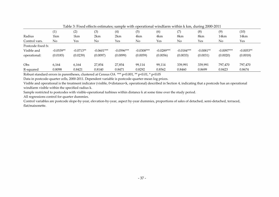
Table 3 reports the results from the postcode fixed effects approach of Strategy A, described in
Section 4.1. This restricts the sample to postcodes which have or will have an operational wind

- 21 -
farm within the specified distance band. Identification comes purely from comparing the change in
postcode prices between the periods before and after the site, with the changes occurring in
postcodes that have already got visible-operational wind farms or which will do so in the future.
Results are reported for 6 radiuses from 1km-14km. The table reports coefficients and standard
errors from the regressions. Standard errors are clustered at Census Output Area level (10 or so
postcodes) to allow for serial correlation in the errors over time and some degree of spatial
correlation in the price changes across neighbouring postcodes. Alternative clustering assumptions
are explored in Table 10 in the Appendix, where the conclusion is that OA level clustering gives
similar results to more general double clustering that allows for serial correlation within postcodes
and cross sectional correlation within quarters. All specifications include a full set of quarterly
dummy variables. There are two columns for each distance category, one in which the
specification includes no other control variables, and the second controlling for the array of
property characteristics and trends described in the methods section. Evidently, controlling for
these property and terrain characteristics makes little difference to the results.
The key finding from this table is that prices in places where wind farms are close and visible are
reduced substantially after a wind farm becomes operational. The price impact is around 7%
within 1km, falling to 6% within 2km, 3% within 4km. Within the 8km or 14km radius, the effect is
less than 1%. These results do not inform us specifically about the visibility impacts of wind farms,
as distinct from other costs and benefits associated with their visibility and operation. These
estimates should be interpreted as the net impact on prices resulting from all channels, including
the potential costs linked to visual impact and noise, and potential benefits of wind farm
proximity. Disentangling visibility from other impacts is left until Section 5.3.

- 22 -
Clearly, interpretation of the estimates in Table 3 as estimates of the causal impact of wind farms
assumes that there are no changes in unobserved housing characteristics coinciding with wind
farms. The results may also be sensitive to pre-existing area specific price trends, that are not
controlled using the various groups of time dummies. Table 4 and Table 5 present some
assessment of these identifying assumptions, based on the sample with the 4km distance threshold
– this being the maximal distance at which there appear to be substantial price effects in Table 3.
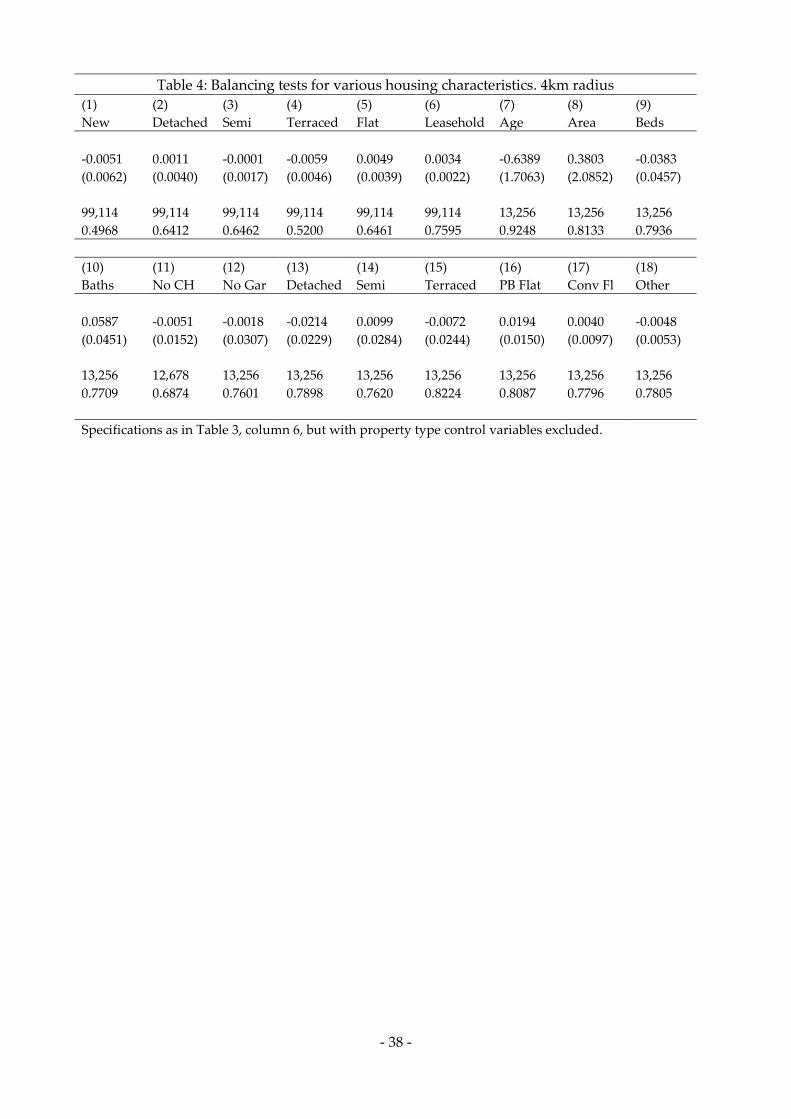
Table 4 presents a series of ‘balancing’ tests in which the dependent variable in the regressions of
Table 3, column 6, is replaced by housing characteristics, and the housing characteristics are
excluded from the set of regressors. The aim here is to see if there are within-postcode changes in
the composition of the sample, in terms of housing characteristics, that coincide with the start of
wind farm operations. Columns (1)-(6) use the few characteristics that are available in the Land
Registry data set. In the remaining columns, mean postcode-by-year characteristics taken from an
auxiliary dataset of transactions from the Nationwide building society are merged to the dataset.
This dataset has far more information on housing characteristics, but is only a sub-set of
transactions, and hence postcodes, in the Land Registry data, therefore the sample size is much
reduced. Looking across Table 4 it is evident that there are no statistically significant changes in
the composition of housing transactions associated with wind farm operation, and there is no
systematic pattern in the point estimates that would suggest that the price changes in Table 3 could
be related to the sale of lower quality houses. The floor area of the property, a potentially
important omitted variable in the land Registry data is in fact positively associated with the wind
farm treatment, though the point estimate (in metres squared) is not large.
Table 5 carries out further robustness tests on the 4km sample, firstly adding in the Nationwide
data set characteristics as control variables (column 2), and replacing the Land Registry prices with
prices from the Nationwide data (column 3) The coefficient estimates from the Nationwide sample

- 23 -
are slightly larger than those from the Land Registry data, although not by much relative to the
standard errors, and changing the source of the price information does not make any difference.
Column (4) adds in additional demographic characteristics from the 2001 Census (proportion not
qualified, proportion tertiary qualified, proportion born in UK, proportion white ethnicity,
proportion employed, proportion in social rented accommodation) interacted with linear time
trend, but again this has no bearing on the results.
Columns (5) shows a specification which controls for region-specific quarterly changes. It is not
feasible to do this simply by including region-by-quarter dummies in the regressions, because
there are too few wind farms becoming operational in any region-quarter period. Instead, the
region-quarter price effects are recovered from a first stage postcode-fixed effects regression of log
prices on region-quarter dummies in the Land Registry dataset, using postcodes beyond the 14km
wind-farm distance limit. The estimated region-quarter effects are then used as controls in the
second stage estimation. Again this has no impact on the key result, even though the region-
quarter effects are strongly correlated with the prices close to the wind farms (the coefficient on the
region-quarter effects is 0.456, with a coefficient of 0.021).
Column (6) does something similar, but controlling for predicted pre-operational linear price
trends in the area defined by the set of postcodes that share the same nearest operational wind
farm within 4km. Again it is not practical to simply include nearest-wind-farm specific trend
variables, since the price changes in response to wind-farm operation are not sharp enough to
successfully identify separately from wind-farm specific price trends over the whole period.
Instead, similarly to the region-quarter trends, the pre-operation wind farm price trends are
estimated in a first stage regression of prices wind farm-specific time trends using observations for
the pre-operation period only. The first stage regression predictions of the wind farms specific

- 24 -
price trends from the pre-operation period are then extrapolated over the whole sample period
and included as controls in the second stage regression. Nothing much changes as a result of this
exercise, although the point estimate is reduced slightly (by around 1 standard error).
Overall, there is no evidence from Table 4 and Table 5 that the finding of negative impacts from
wind farms on prices arises from omitted variables or unobserved price trends.
More detail on distance-decay of the wind farm price effects within the 14km limit is provided in
Table 6. Here the sample is postcodes with transactions within 14km of a site, and the treatment
indicators for the different distance bands are included in the same regression. The coefficients
indicate the effects at each distance band within this 14km radius. As before Column (1) includes
just quarterly dummies, whereas Column (2) includes the full set of control variables, including
distance-band-by-year dummies. The results are broadly in line with the alternative presentation
in Table 3. The price effect within 1km, and at 1-2km is around 5.5-6%. This falls quite sharply in
the 2-4km distance band, to 1.9%. Beyond this there are price effects right out as far as 14km,
although these are small at around 1%.
5.2 Strategy B placebo results
Section 4.2 described extensions to the analysis that compares the price effects of operational
turbines with the price effects of planned, but undeveloped wind farms that are not yet
constructed. The distribution of these planned wind farms is shown in Figure 3. The regression
results relating to planned and refused wind farm developments are shown in Table 7. The sample
includes postcodes within the specified distance of sites that are operational by the end of the
study period (same samples as Table 3) plus postcodes within the specified distance of sites that
are in planning by the end of the study period. The purpose of these results is to assess whether
the patterns in Table 3 could arise from endogenous spatial targeting of wind farms.

- 25 -
Looking across Table 7, the same pattern of results for visible-operational wind farms emerges as
in Table 3 (which is the case by construction – the coefficients are basically identified from the
same variation as in Table 3). By contrast the coefficients on the placebo ‘planning ‘treatment are
statistically insignificant and small in magnitude relative to the operational effects, in the distance
bands close to the wind farm sites. There are, however, small positive, significant effects in the
larger samples corresponding to the bigger distances. There is no clear causal explanation for these
patterns, given that the planning events are randomly allocated across time within postcodes. A
potential explanation is that the before-after planning treatment indicator is picking up
interactions between non-linear postcode-specific unobserved price trends and the postcode fixed
effects, which may not successfully be controlled for by postcode fixed effects and the time trend
dummies included in the regressions. Whatever the explanation, the effects are opposite in sign to
those for operational turbines, so do not appear to be a cause of the patterns seen for the effects of
operational turbines.
The distance decay of the price effects for operational, as compared to planned wind farms is
illustrated in Figure 4. The figure plots the coefficients from regressions of the type shown in Table
6 for visible operational wind farms, but with the addition of the ‘placebo’ treatment effects for the
planned wind farms. The sample includes postcodes which have visible-operational wind farms or
visible-planned wind farms within 14km by the end of the period. In this distance-band set up
there is no evidence of statistically significant effects of any magnitude from the placebo
treatments. The final row presents a difference-in-difference-in-difference comparison between the
visible-operational and visible-planned treatment effects, which are virtually identical to the
results in Table 6.

- 26 -
5.3 Strategy C results
The methods described in 4.3 proposed comparing the price effects in postcodes with visible-
operational turbines to the price effects in postcodes with non-visible operational turbines. To
illustrate the basis for Strategy C, Figure 5 shows the viewshed for a wind farm in north east
England. This is the Haswell Moor wind farm in County Durham, which has 5 turbines, a total
capacity of 10MW and the height to the tip of the turbines is 110m. This is a fairly typical wind
farm development in the sample. The dark shaded areas are residential postcodes and the light
grey shading indicates the land where at least the tips of the turbine blades are visible (technically,
these are computed as the land surface that is visible to an observer at the tip of the turbine).
Strategy C is compares prices changes occurring with the start of wind farm operation in postcodes
where the turbines are visible, with those occurring where they are not-visible.
The results for different distance radii are shown in Table 8. This is presented in the same way as
Table 7, but allowing for effects from non-visible operational wind farms rather than planned wind
farms. The sample includes postcodes with visible-operational turbines and non-visible
operational turbines within each distance band by the end of the period. All regressions include
the usual controls for trends and differences in topography, and allow for differences in general
time patterns between postcodes where operational turbines will become visible and postcodes
where they do not. Note that it is infeasible to compare visible and non-visible wind-farms within
the 1km distance band as there almost no cases where turbines are not visible at this distance, so
the 1km results are missing. Otherwise, the usual pattern is seen in the coefficients for visible-
operational turbines, but the effects in areas close to operational turbines where these are not
visible is quite different. The point estimates within the 2km band are similar to those for visible-
operational turbines, but statistically insignificant. Again, an issue here is that there are relatively
few cases where turbines are not visible at a postcode if they are this close, and the classification

- 27 -
into visible and non-visible cases is potentially very noisy, given the 200m resolution of the
viewshed (and the fact that a person probably does not have to move far from there house to
observe turbines at this distance, even if they are obscured from view at the house itself). Further
out, a more interesting pattern emerges: within 4km there is no effect on prices from operational
turbines that are not visible, which begins to suggest that the effects from visible-operational
turbines are largely attributable to visibility. Within 8km, and at bigger radii around the wind farm
site, small significant positive price effects start to emerge, whilst the effects in postcodes with
wind turbine visibility remain negative. Again, the results for distance bands are presented
graphically in Figure 6, to show the distance decay pattern, and the offsetting effects of visibility
and non-visibility are clearly evident (except within the 1km band where the estimates for non-
visibility are too imprecise).
One potential explanation for these contrasting effects is that wind farms provide some general
benefits in the local area, due to community donations, shares in profits, other local area
enhancement schemes and rents to land owners. There may also be wage and employment
benefits. In this case, the basic price effects estimated from the visible-operational treatment
dummies under-estimate the marginal willingness to pay to avoid the visual dis-amenity, because
these are in part already compensated by higher wages or other benefits (as in the classic wage-
price-amenity trade off in the Roback model of compensating wage and land price disparities,
(Roback 1982). An alternative interpretation is that housing market frictions create very localised
housing markets, and construction of turbines therefore restricts the availability of housing
without views of the turbines, thus raising the price of postcodes without visibility relative to
those where the turbines are visible. Unfortunately, it is not possible to distinguish between these
two hypotheses in the current set up. Either way, the willingness to pay to avoid visibility should
be estimated by the difference between the coefficients on the visible-operational treatment

- 28 -
dummies and the non-visible operational treatment dummies. These difference-in-difference-in-
difference estimates are shown at the bottom of Figure 6, and indicate a visibility impact of around
2.6% from 2km out to 8km. Beyond 8km there is no effect from the average wind farm, and below
2km no effect is detectable due the lack of clear distinction in visibility at this distance.
5.4 Further results on numbers of turbines.
The results so far have looked simply at turbine development as a binary treatment effect, and
have ignored the scale of the wind farm. Table 9 investigates the whether there is a greater cost
associated with larger developments with more turbines, and over what distance. The setup is
basically the same as in Table 6, but with interactions between dummies for wind farm size and
distance. The results are in line with what would be expected if the price impacts are related to the
dis-amenity of wind farm visibility. Bigger wind farms have a bigger impact on prices at all
distances. A wind farm with 20+ turbines within 2km reduces prices by some 11% on average.
Note though that a postcode within 2km of the centroid of a 20+ turbine windfarm could be almost
at the turbine field, so this price effect could relate to noise and visual flicker problems, and is quite
clearly an extreme case. However, even at 8-14km there is a 3.7% reduction in prices associated
with large visible operational wind farms. Medium size wind farms above average size also have
strong effects throughout the distance range, falling from 5.7% within 2km to just over 1% by
14km. The effect of smaller wind farms with less than 1-10 turbines is, as might be expected,
concentrated in the first 2km where there is a 5% reduction in prices, falling to just over 1% at 4km
and becoming smaller and/or insignificant beyond that.
The possibility of using other planning events was discussed in Section 4.4. Figure 7 shows
findings related to the impacts of wind farm planning refusal, using the same distance band set up
of Figure 4 , but with postcodes with potentially visible wind farms that were refused planning

- 29 -
permission, alongside the usual visible-operational cases. The results are quite surprising. Refusal
events seem to be associated with positive price effects, and these are very large close to the
proposed wind farm locations. One potential explanation for these positive impacts is that refusal
of planning permission may trigger price effects, if it signals to home owners and buyers that the
local planning authority will be unwilling to proceed with future wind farm developments in the
local area.
It is also possible that places where wind farms were refused permission were the subject of
vigorous local campaigning, and these campaigns may have lowered prices prior to refusal – e.g.
because local residents tried to sell quickly, or because the campaigns raised awareness amongst
potential buyers. The positive effects from refusal of permission may therefore represent some
bounce back of prices to pre-planning levels. Of course if similar effects were observed during the
planning and pre- approval periods for operational wind farms, the results presented so far could
underestimate of the impact of visible operational wind farms, because there is a pre-operation dip
in prices in response to the planning process, and this will reduce the estimated pre-post operation
price differential. In this case the refusal effects are, in effect, the mirror image of the effect of wind
farm planning on local prices (which it is not possible to estimate directly, for reasons discussed in
4.2).
Under either of these assumptions, the difference-in-difference-in-difference estimates implicit in
the graph in Figure 7 might provide better estimates of the effects of wind farm operation relative
to the re-planning stage. These estimates are shown at the bottom of the figure, and are
substantially bigger than the baseline estimates of visible operational turbines in Table 6 and
elsewhere in this paper. Given the uncertainties in interpretation, these estimates are best treated
as an upper bound to the potential impacts.

- 30 -
6 Conclusions
The paper has estimated the effects of visible wind farm turbines on housing prices in England and
Wales. The study used a micro-aggregated postcode-by-quarter panel of housing transactions
spanning 12 years, and estimated difference-in-difference effects using a postcode fixed effects
based methodology. Comparisons were made between postcodes in which turbines became
operational and visible with various control groups. All the results point in the same direction,
regardless of the specific research design. Wind farms reduce house prices in postcodes where the
turbines are visible. This price reduction is around 5-6% for housing with a visible wind farm of
average size (11 turbines) within 2km, falling to 3% within 4km, and to 1% or less by 14km which
is at the limit of likely visibility.
Evidence from comparisons with places close to wind farms, but where wind farms are less visible
suggests that most if not all of these price reductions are directly attributable to turbine visibility.
The effects of wind farms on the prices of locations with limited visibility are statistically
insignificant or even positive – providing some indication that wind farms generate some local
benefits, though these are more than offset by the dis-amenity associated with visibility. This may
be why previous studies that have failed to distinguish between places where nearby turbines are
visible and places where they are not, have failed to find effects. As might be expected, the effects
are bigger and have greater geographical spread for larger wind farms. Wind farms with 20 or
more turbines reduce prices by 3% at distances between 8-14km, and by up to 12% within 2km.
The paper presents a number of robustness tests, but even so the findings should be interpreted
with some ‘health warnings’. The information on wind farm location and visibility is limited by
lack of data on the precise location of individual turbines, so the classification of postcodes in
terms of visibility is subject to measurement error. This is most likely to result in some attenuation

- 31 -
of the estimated effects. Steps were taken to minimise this problem by eliminating postcodes
where visibility is ambiguous. More importantly, the data lacks historical information on the
timing of events leading up to wind farm operation (announcement, approval, construction etc.) so
the price effects reported here relate to the difference between the post-operation and pre-
operation periods, for the periods spanned by the data. However, the wind farm development
cycle can last a number of years, and price changes evolve fairly slowly over time in response to
events. Again the most likely consequence of this is that the results underestimate the full impact
between the pre-announcement and post-construction phase. Results based on comparison of
operational sites and those refused planning permission suggest that these full impacts could be
much bigger – the upper-bound estimate is about 15% within 2km of the average wind farm.
Further data collection effort is required to fully address these issues.
Well established theories (Rosen 1974) suggest that these price effects can be interpreted as
marginal willingness to pay to avoid the dis-amenity associated with wind farm proximity and
visibility, net of any benefits provided by the wind farms in terms of economic opportunities,
community payments or other financial compensation. If we take the figures in the current paper
seriously as estimates of the mean willingness to pay to avoid wind farms in communities exposed
to their development, the implied costs are quite substantial. For example, a household would be
willing to pay around £600 per year to avoid having a wind farm of average size visible within
2km, or would be willing to pay around £200 per year to avoid having a large wind farm visible
within 8-14km.7 The implied amounts required per wind farm to compensate households for their
loss of visual amenities is therefore fairly large: about £12 million for a typical 11 turbine wind
7 This is based on an average house price of £140,000, a 3% price reduction and a 5% interest rate

- 32 -
farm, based on the average numbers of households with turbines currently visible within 4km.8
The corresponding values for large wind farms will be much higher than this, as their impact is
larger and spreads out over much greater distances.
These per-household figures are comparable to the highest estimates from the stated preference
literature. The figures cited in Bassi, Bowen and Fankhauser (2012) are typically much less than
£100 per year, though this is per individual, so household willingness to pay could be higher. It is
worth noting, however, that the revealed preference method based on housing markets elicits the
preferences of marginal home owners in the areas close to wind farms, which may differ from the
mean willingness to pay amongst all households in the population.
8 Based on: around 1.8% of postcodes within 4km of a visible turbine; the number of households in England and Wales is
23.4 million; the capitalised effect of visibility within 4km is 3%; the average house price is £140000; and the number of
operational turbines is 148.

- 33 -
References
Bell, Derek, Tim Gray & Claire Haggett (2005), The ‘Social Gap’ in Wind Farm Siting
Decisions: Explanations and Policy Responses Environmental Politics, 14 (4) 460 – 477
Busso, Matias, Jesse Gregory & Patrick Kline (2013) Assessing the Incidence and Efficiency of
a Prominent Place Based Policy, American Economic Review, American Economic
Association 103(2) 897-947
DECC (2013a) Digest of United Kingdom Energy Statistics, Chapter 6: Renewable sources of
energy, Department of Energy & Climate Change, London
DECC (2013b) Digest of United Kingdom Energy Statistics, Internet Booklet,
https://www.gov.uk/government/uploads/system/uploads/attachment_data/file/225056/
DUKES_2013_internet_booklet.pdf, accessed November 2013
European Commission (2006) Energy Technologies: Knowledge – Perception – Measures,
European Union Community Research Report, Luxembourg: Office for Official
Publications of the European Communities
Hoen, Ben, Jason P. Brown, Thomas Jackson, Ryan Wiser, Mark Thayer and Peter Cappers
(2013) A Spatial Hedonic Analysis of the Effects of Wind Energy Facilities on
Surrounding Property Values in the United States, Environmental Energy Technologies
Division, Ernest Orlando Lawrence Berkeley National Laboratory, LBNL-6362E
Hoen, Ben, Ryan Wiser, Peter Cappers, Mark Thayer, and Gautam Sethi (2011), Wind Energy

- 34 -
Facilities and Residential Properties: The Effect of Proximity and View on Sales Prices,
Journal of Real Estate Research
Moulton, Brett (1990) An Illustration of a Pitfall in Estimating the Effects of Aggregate
Variables on Micro Units, The Review of Economics and Statistics Vol. 72, No. 2, May,
1990
Munday, Max, Gill Bristow, Richard Cowell, Wind farms in rural areas: How far do
community benefits from wind farms represent a local economic development
opportunity? Journal of Rural Studies 27 1-12
Roback , Jennifer (1982), Wages, Rents, and the Quality of Life, The Journal of Political
Economy, 90 (6) 1257-1278.
Rosen, Sherwin (1974) Hedonic Prices and Implicit Markets: Product Differentiation in Pure
Competition, The Journal of Political Economy, 82 (1) 34-55
Samuela Bassi, Alex Bowen and Sam Fankhauser (2012) The case for and against onshore
wind energy in the UK, Grantham Research Institute on Climate Change and
Environment Policy Brief, London
Thompson, Samuel (2011) Simple Formulas for Standard Errors that Cluster by Both Firm and
Time, Journal of Financial Economics, 99 1–10
University of Newcastle (2002) Visual Assessment of Windfarms Best Practice. Scottish
Natural Heritage Commissioned Report F01AA303A.
Vidal, John (2012) Wind turbines bring in 'risk-free' millions for rich landowners, Guardian

- 35 -
28th February online http://www.theguardian.com/environment/2012/feb/28/windfarms-
risk-free-millions-for-landowners, accessed November 2013
Bakker, R.H., E. Pedersen, G.P. van den Berg, R.E. Stewart, W. Lok, J. Bouma (2012) Effects of
wind turbine sound on health and psychological distress, Science of the Total
Environment, 425 42–51.
Farbouda, A., R. Crunkhorna and A Trinidadea (2013), ‘Wind turbine syndrome’: fact or
fiction? The Journal of Laryngology & Otology, 127 (03) 222-226

- 36 -
Table 1: Windfarm summary data, 1992-2011 England and Wales
Mean s.d. Min Max
Operational
Turbines mean 11.2 15.4 1 103
Turbines median 6
MW capacity 18.6 39.2 .22 300
Height to tip 90.9 29.2 42 150
Offshore 14
Forest 8
Farm 82
Wild 39
Coast 5
Status
Operational 148
Approved 61
Construction 10
Planning 160
Refused 57
Withdrawn 34
Table 2: Main estimation sample summary data, 2000-2011 England and Wales
Visible-operational turbines within 14km
Mean s.d.
Log price 11.542 0.654
New build 0.043 0.197
Detached house 0.261 0.428
Semi-detached house 0.065 0.24
Terraced house 0.332 0.455
Flat/Maisonette 0.342 0.462
Freehold 0.859 0.34
Proportion with visible turbines within 1km 0.004 0.062
Proportion with visible turbines within 1-2km 0.014 0.119
Proportion with visible turbines within 2-4km 0.046 0.210
Proportion with visible turbines within 4-8km 0.158 0.365
Proportion with visible turbines within 8-14km 0.306 0.461
Obs 797470
- 37 -
Table 3: Fixed effects estimates; sample with operational windfarm within k km, during 2000-2011
(1) (2) (3) (4) (5) (6) (7) (8) (9) (10)
Radius 1km 1km 2km 2km 4km 4km 8km 8km 14km 14km
Control vars. No Yes No Yes No Yes No Yes No Yes
Postcode fixed fx
Visible and -0.0539** -0.0713** -0.0601*** -0.0596*** -0.0308*** -0.0289*** -0.0184*** -0.0081** -0.0097*** -0.0053**
operational: (0.0185) (0.0239) (0.0097) (0.0099) (0.0059) (0.0056) (0.0033) (0.0031) (0.0020) (0.0018)
Obs 6,164 6,164 27,854 27,854 99,114 99,114 339,991 339,991 797,470 797,470
R-squared 0.8098 0.8421 0.8140 0.8471 0.8292 0.8562 0.8460 0.8699 0.8423 0.8674
Robust standard errors in parentheses, clustered at Census OA *** p<0.001, ** p<0.01, * p<0.05
Data in postcode-quarter cells, 2000-2011. Dependent variable is postcode-quarter-mean log prices.
Visible and operational is the treatment indicator (visible, 0<distance<k, operational) described in Section 4, indicating that a postcode has an operational
windfarm visible within the specified radius k.
Sample restricted to postcodes with visible-operational turbines within distance k at some time over the study period.
All regressions control for quarter dummies.
Control variables are postcode slope-by-year, elevation-by-year, aspect by-year dummies, proportions of sales of detached, semi-detached, terraced,
flat/maisonette.
- 38 -
Table 4: Balancing tests for various housing characteristics. 4km radius
(1) (2) (3) (4) (5) (6) (7) (8) (9)
New Detached Semi Terraced Flat Leasehold Age Area Beds
-0.0051 0.0011 -0.0001 -0.0059 0.0049 0.0034 -0.6389 0.3803 -0.0383
(0.0062) (0.0040) (0.0017) (0.0046) (0.0039) (0.0022) (1.7063) (2.0852) (0.0457)
99,114 99,114 99,114 99,114 99,114 99,114 13,256 13,256 13,256
0.4968 0.6412 0.6462 0.5200 0.6461 0.7595 0.9248 0.8133 0.7936
(10) (11) (12) (13) (14) (15) (16) (17) (18)
Baths No CH No Gar Detached Semi Terraced PB Flat Conv Fl Other
0.0587 -0.0051 -0.0018 -0.0214 0.0099 -0.0072 0.0194 0.0040 -0.0048
(0.0451) (0.0152) (0.0307) (0.0229) (0.0284) (0.0244) (0.0150) (0.0097) (0.0053)
13,256 12,678 13,256 13,256 13,256 13,256 13,256 13,256 13,256
0.7709 0.6874 0.7601 0.7898 0.7620 0.8224 0.8087 0.7796 0.7805
Specifications as in Table 3, column 6, but with property type control variables excluded.

- 39 -
Table 5: Robustness to additional control variables and trends. 4km radius
(1) (2) (3) (4) (5)
Baseline
estimate
from Table
3
Sub-sample
with
additional
Nationwide
property Xs
Nationwide
prices and
Xs
Census
output area
Xs x trends
Control for
regional
trends from
from full
dataset
Control for
pre-
operational
nearest
wind farm
trends
Visible operational -0.0289*** -0.0463** -0.0405*** -0.0275*** -0.0272*** -0.0219***
turine within 4km (0.0056) (0.0145) (0.0120) (0.0057) (0.0052) (0.006)
Observations 99,114 12,678 12,678 93,510 99,114 99114
R-squared 0.8562 0.8913 0.9768 0.8383 0.8582 0.857
Robust standard errors in parentheses, clustered at Census OA *** p<0.001, ** p<0.01, * p<0.05
Column 2 controls for floor size, number of bedrooms, bathrooms, central heating type, garage type, and
detailed property type for postcodes represented in Nationwide data. Column 3 similar, using price reported
in Nationwide data. Column 3 adds linear trends interacted with census 2001 variables at output area (OA)
level (OA land area, proportion with no qualifications, proportion with tertiary qualifications, proportion
born UK, proportion white ethnicity, proportion employed, proportion in social rented housing).
Column 5 controls for piecewise constant quarterly price trends predicted from transactions beyond 14km
from any windfarm, operational, planned or refused (coefficient on predicted prices 0.456 (0.021).
Column 6 controls for nearest operational windfarm linear time trends estimated from pre-operational
period (coefficient on predicted prices 0.103 (0.014).
Specifications otherwise as Table 3, column 6,
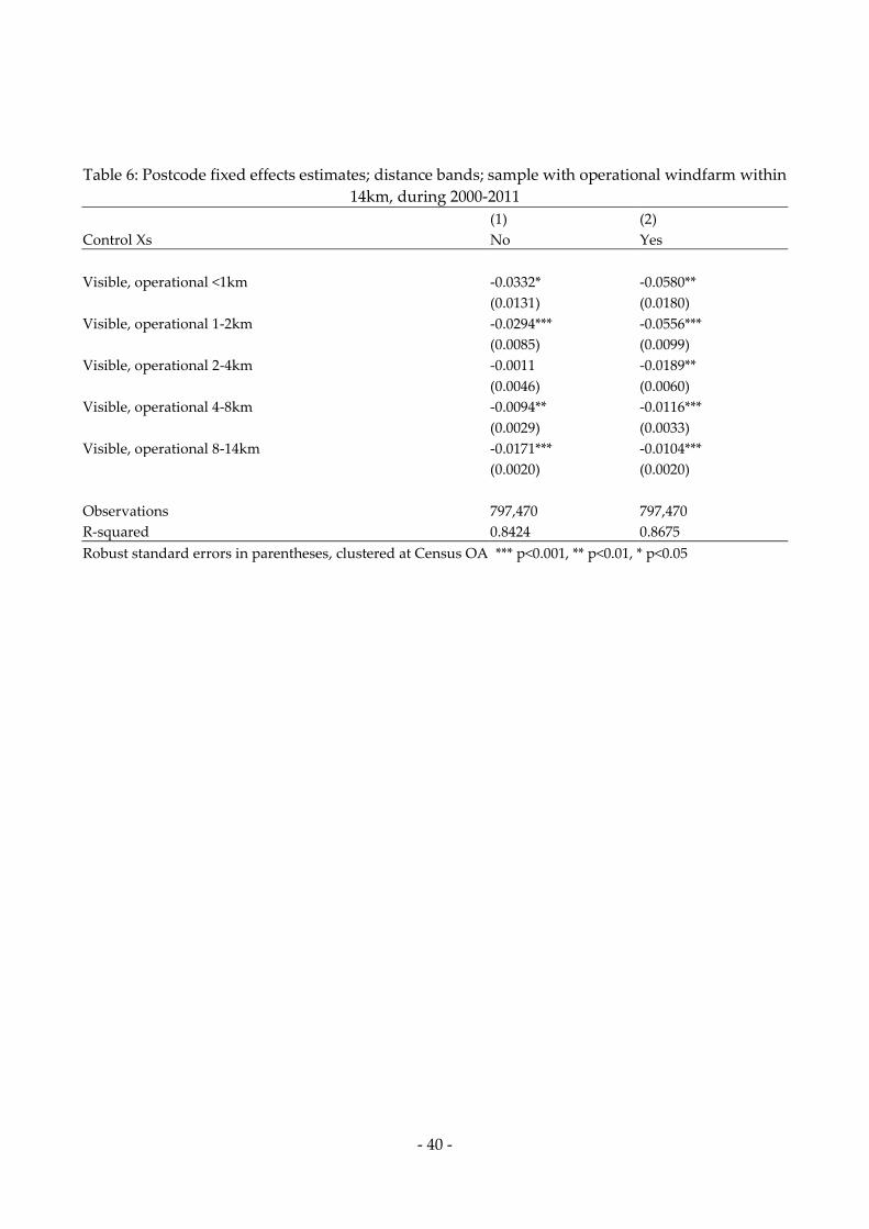
- 40 -
Table 6: Postcode fixed effects estimates; distance bands; sample with operational windfarm within
14km, during 2000-2011
(1) (2)
Control Xs No Yes
Visible, operational <1km -0.0332* -0.0580**
(0.0131) (0.0180)
Visible, operational 1-2km -0.0294*** -0.0556***
(0.0085) (0.0099)
Visible, operational 2-4km -0.0011 -0.0189**
(0.0046) (0.0060)
Visible, operational 4-8km -0.0094** -0.0116***
(0.0029) (0.0033)
Visible, operational 8-14km -0.0171*** -0.0104***
(0.0020) (0.0020)
Observations 797,470 797,470
R-squared 0.8424 0.8675
Robust standard errors in parentheses, clustered at Census OA *** p<0.001, ** p<0.01, * p<0.05

- 41 -
Table 7: Postcode fixed effects estimates; comparisons of operational windfarms with planned
windfarms within k km, during 2000-2011
(1) (2) (3) (4) (5)
Radius 1km 2km 4km 8km 14km
Control Xs Yes Yes Yes Yes Yes
Operational -0.0770*** -0.0595*** -0.0183** -0.0095** -0.0054**
(0.0218) (0.0103) (0.0060) (0.0032) (0.0020)
Planned -0.0153 0.0042 0.0049 0.0117*** 0.0109***
(0.0165) (0.0078) (0.0043) (0.0028) (0.0018)
Obs. 11,117 50,754 169,237 506,208 1,085,839
R-squared 0.8480 0.8585 0.8656 0.8706 0.8684
Robust standard errors in parentheses, clustered at Census OA *** p<0.001, ** p<0.01, * p<0.05
Table 8: Postcode fixed effects estimates; comparisons of visible operational windfarms with non-
visible operational windfarms within k km, during 2000-2011
(1) (2) (3) (4) (5)
Radius 1km 2km 4km 8km 14km
Control Xs
Yes Yes Yes Yes
Operational visible - -0.0596*** -0.0274*** -0.0074* -0.0059***
(0.0099) (0.0056) (0.0030) (0.0018)
Operational - -0.0688 0.0059 0.0162*** -0.0117***
not visible (0.0630) (0.0133) (0.0042) (0.0021)
Obs. - 28,951 116,595 508,147 1,391,879
R-squared - 0.8498 0.8578 0.8712 0.8685
Robust standard errors in parentheses, clustered at Census OA *** p<0.001, ** p<0.01, * p<0.05

- 42 -
Table 9: Effects by windfarm size and distance bands
(1) (2) (3) (4)
<2km 2-4km 4-8km 8-14km
1-10 turbines -0.0531*** -0.0153* -0.0031 -0.0057**
(0.0091) (0.0061) (0.0035) (0.0022)
11-20 turbines -0.0565** -0.0321*** -0.0483*** -0.0117***
(0.0189) (0.0097) (0.0059) (0.0035)
20+ turbines -0.1163*** -0.0568*** -0.0593*** -0.0276***
(0.0284) (0.0171) (0.0063) (0.0030)
Obs. 797469. R-squared 0.8676
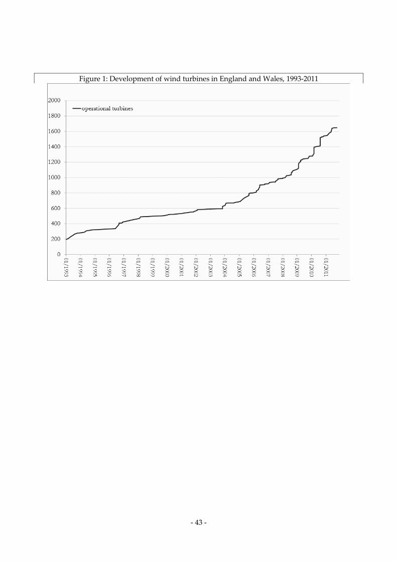
- 43 -
Figure 1: Development of wind turbines in England and Wales, 1993-2011
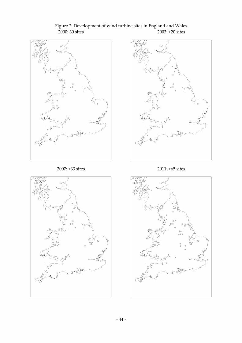
- 44 -
Figure 2: Development of wind turbine sites in England and Wales
2000: 30 sites 2003: +20 sites
2007: +33 sites 2011: +65 sites
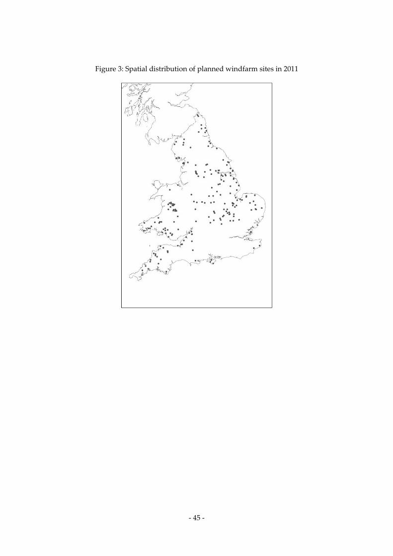
- 45 -
Figure 3: Spatial distribution of planned windfarm sites in 2011
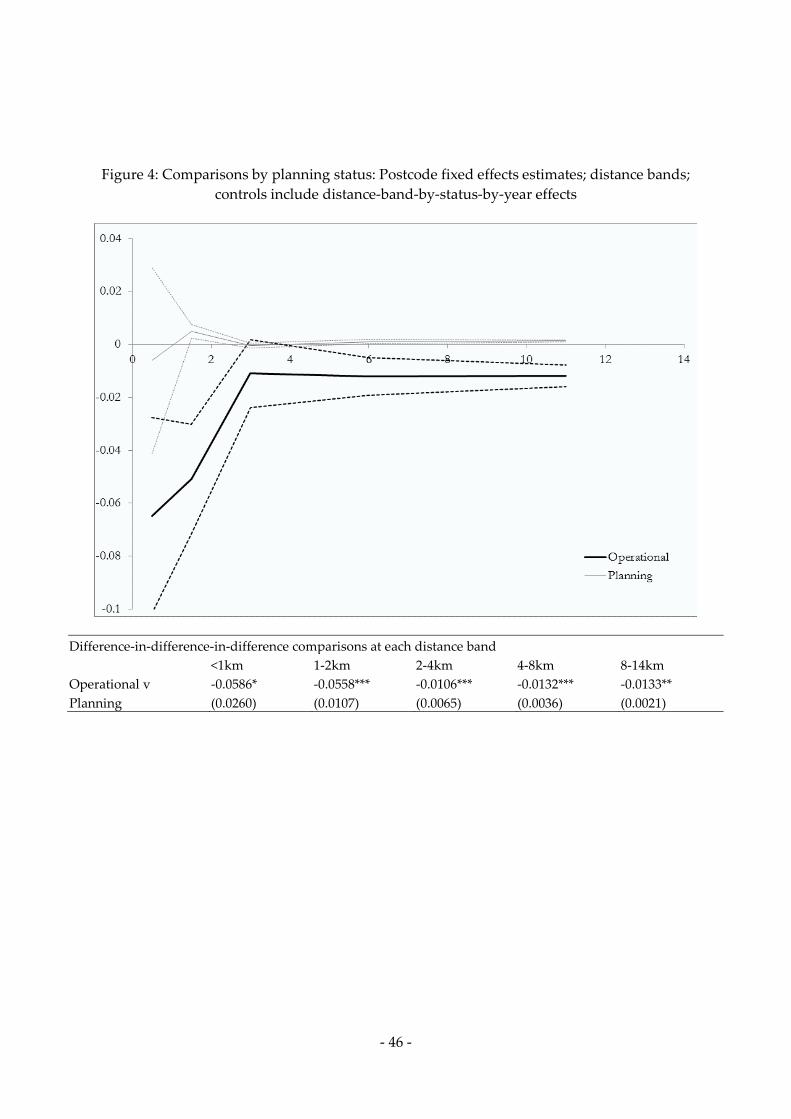
- 46 -
Figure 4: Comparisons by planning status: Postcode fixed effects estimates; distance bands;
controls include distance-band-by-status-by-year effects
Difference-in-difference-in-difference comparisons at each distance band
<1km 1-2km 2-4km 4-8km 8-14km
Operational v -0.0586* -0.0558*** -0.0106*** -0.0132*** -0.0133**
Planning (0.0260) (0.0107) (0.0065) (0.0036) (0.0021)
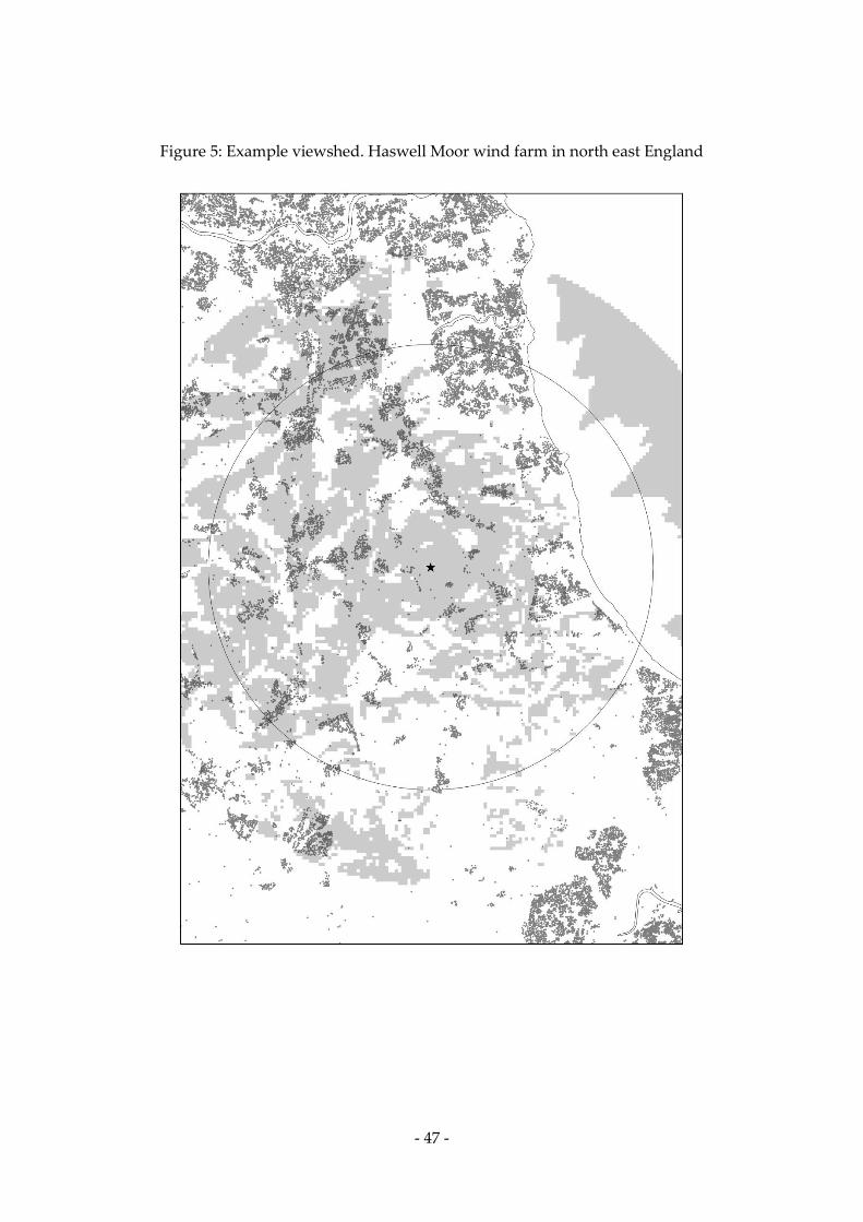
- 47 -
Figure 5: Example viewshed. Haswell Moor wind farm in north east England
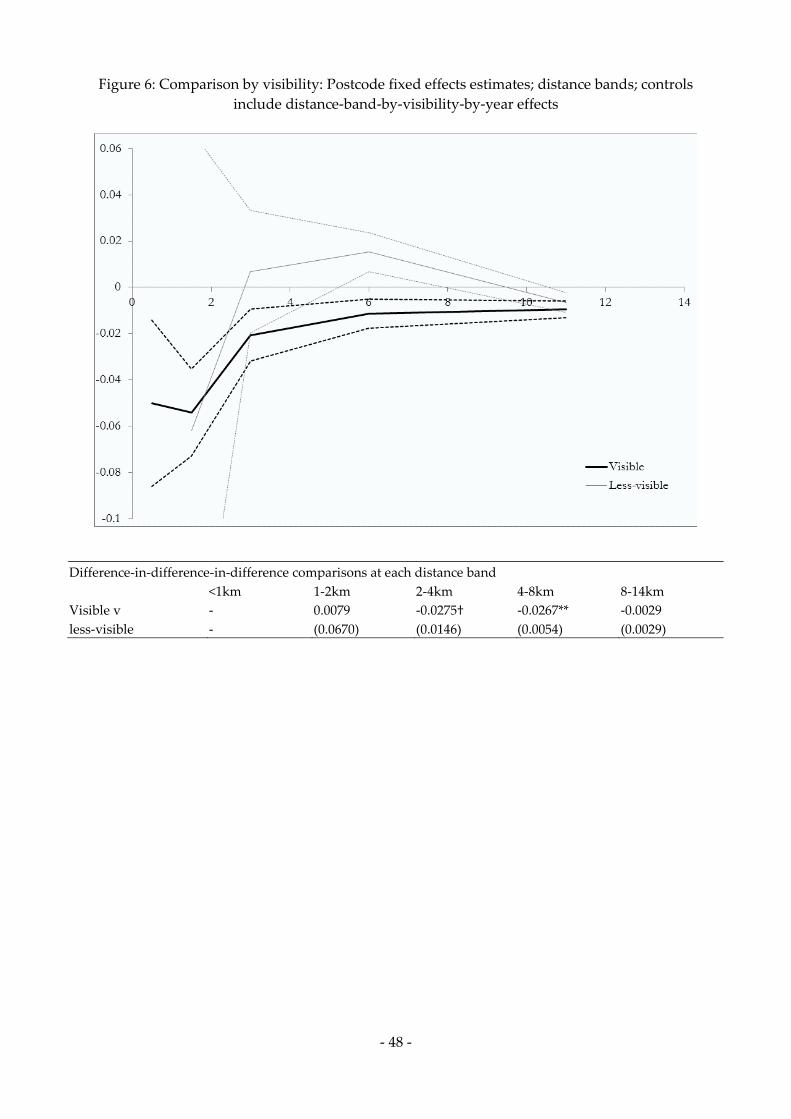
- 48 -
Figure 6: Comparison by visibility: Postcode fixed effects estimates; distance bands; controls
include distance-band-by-visibility-by-year effects
Difference-in-difference-in-difference comparisons at each distance band
<1km 1-2km 2-4km 4-8km 8-14km
Visible v - 0.0079 -0.0275† -0.0267** -0.0029
less-visible - (0.0670) (0.0146) (0.0054) (0.0029)

- 49 -
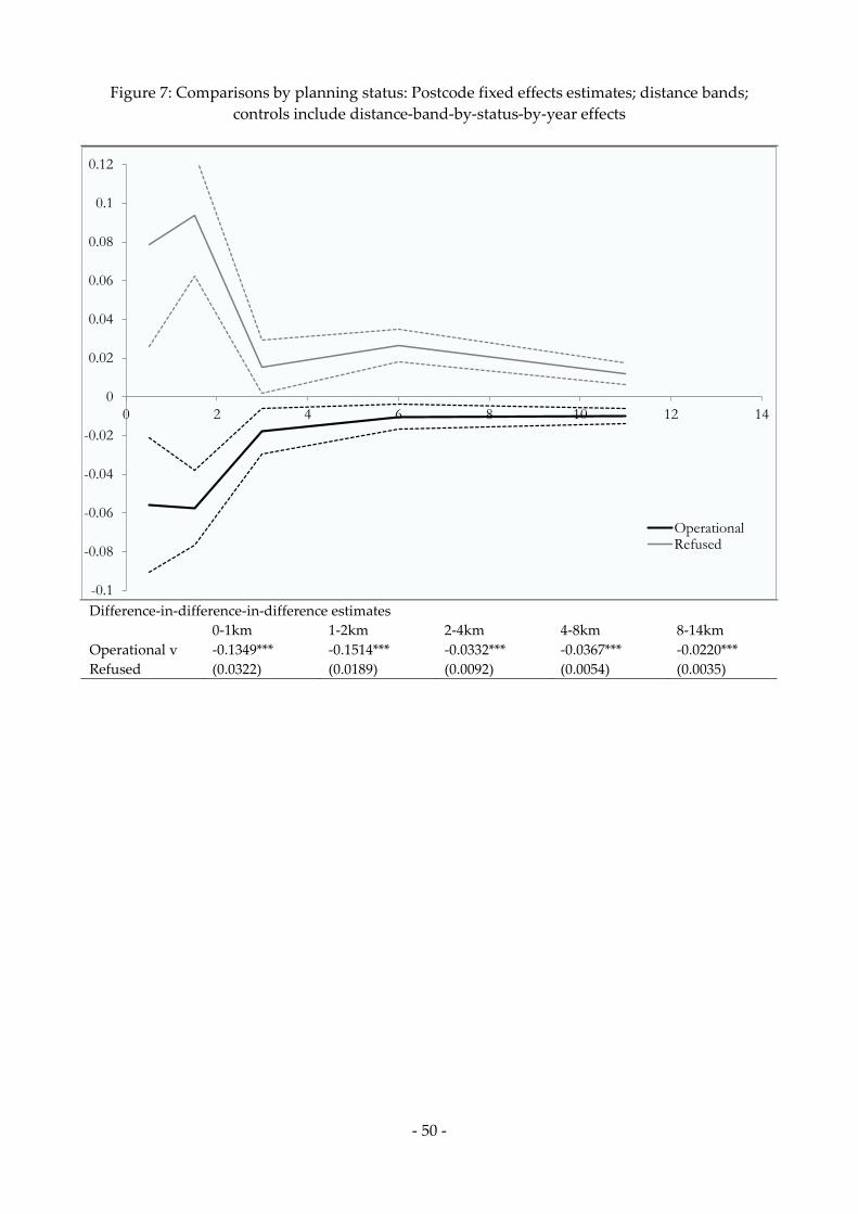
- 50 -
Figure 7: Comparisons by planning status: Postcode fixed effects estimates; distance bands;
controls include distance-band-by-status-by-year effects
Difference-in-difference-in-difference estimates
0-1km 1-2km 2-4km 4-8km 8-14km
Operational v -0.1349*** -0.1514*** -0.0332*** -0.0367*** -0.0220***
Refused (0.0322) (0.0189) (0.0092) (0.0054) (0.0035)
-0.1
-0.08
-0.06
-0.04
-0.02
0
0.02
0.04
0.06
0.08
0.1
0.12
0 2 4 6 8 10 12 14
OperationalRefused

- 51 -
7 Appendix
There are potential concerns over the standard errors of the estimates presented in the main
results, because the regression unobservables are potentially correlated over space in unknown
ways, and are undoubtedly serially correlated within postcodes. As is well known (Moulton 1990),
the standard errors on aggregated treatment variables can be downward biased when there is
serial and/or spatial correlation in the regression error terms, although in the current application
the treatment is by its nature aggregated. In the current analysis the treatment is constructed at
postcode level, although the effect is aggregated across postcodes within the distance bands in
Table 6 for each wind farm, since when a windfarm is built it affects visibility in all postcodes
within that distance band. Of course this is a genuine effect due to the geographical level of the
treatment, not an arbitrary geographical aggregation of micro level interventions, so the Moulton
example does not necessarily apply exactly.
The usual adjustment for this kind of problem is to use ‘clustered’ standard errors at the level of
the treatment - i.e. distance band-by-windfarm clusters in the current example - though in this case
this would be an extremely conservative assumption, since it assumes, in effect that the errors are
perfectly correlated both within a distance band, both in the cross section and over time. An
equivalent evaluation of a national policy would dictate a single cluster, which is clearly a silly
assumption. On the other hand, when researchers use fixed effect estimators, they generally cluster
at the level of the fixed effects – i.e. postcodes in this case - to allow for serial correlation within the
erros within panel units. The standard errors reported in the main results cluster at Census output
area (OA) level, but given the uncertainty over the appropriate level, Table 10 in the Appendix
explores a range of clustering options, using the specification of Table 6.
The first column reports the standard errors with OA level clusters. The second column clusters at
groups define by the distance-band, the identifier of the nearest windfarm and the time period
(quarter) allowing for cross sectional spatial error autocorrelation or heteroscedasticity across these
groups. The standard errors are smaller in this case. The next column allows for clusters both at
postcode level (to allow for serial correlation within panel units) and for each quarter (allowing for
correlation across all panel units within each period).9 These standard errors are close to those
estimated using OA clusters, and seem likely to account for most plausible sources of bias in the
standard errors.
The remaining columns adopt other more conservative assumptions. Column 4 expands to Census
ward clusters, allowing for cross sectional and serial correlation within census wards, which
doubles the standard errors, although the coefficients remain significant witn the 0-1 and 1-2 km
bands. Finally, the last column adopts the most conservative clustering assumption and allows for
arbitrary correlation over time and in the cross section within wind-farm-by-distance-band-
groups. The estimates in the 0-1km and 1-2km bands are still significant, if only at the 10% level.
9 Using the method of Thompson (2011).
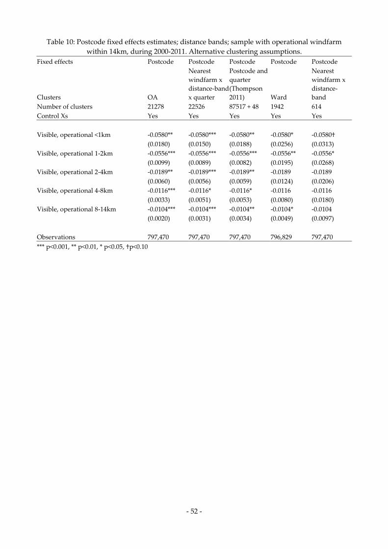
- 52 -
Table 10: Postcode fixed effects estimates; distance bands; sample with operational windfarm
within 14km, during 2000-2011. Alternative clustering assumptions.
Fixed effects Postcode Postcode Postcode Postcode Postcode
Clusters OA
Nearest
windfarm x
distance-band
x quarter
Postcode and
quarter
(Thompson
2011) Ward
Nearest
windfarm x
distance-
band
Number of clusters 21278 22526 87517 + 48 1942 614
Control Xs Yes Yes Yes Yes Yes
Visible, operational <1km -0.0580** -0.0580*** -0.0580** -0.0580* -0.0580†
(0.0180) (0.0150) (0.0188) (0.0256) (0.0313)
Visible, operational 1-2km -0.0556*** -0.0556*** -0.0556*** -0.0556** -0.0556*
(0.0099) (0.0089) (0.0082) (0.0195) (0.0268)
Visible, operational 2-4km -0.0189** -0.0189*** -0.0189** -0.0189 -0.0189
(0.0060) (0.0056) (0.0059) (0.0124) (0.0206)
Visible, operational 4-8km -0.0116*** -0.0116* -0.0116* -0.0116 -0.0116
(0.0033) (0.0051) (0.0053) (0.0080) (0.0180)
Visible, operational 8-14km -0.0104*** -0.0104*** -0.0104** -0.0104* -0.0104
(0.0020) (0.0031) (0.0034) (0.0049) (0.0097)
Observations 797,470 797,470 797,470 796,829 797,470
*** p<0.001, ** p<0.01, * p<0.05, †p<0.10
Recommended