GMS Equations From Irreversible
ThermodynamicsChEn 6603
References• E. N. Lightfoot, Transport Phenomena and Living Systems, McGraw-Hill, New York 1978.
• R. B. Bird, W. E. Stewart and E. N. Lightfoot, Transport Phenomena 2nd ed., Chapter 24 McGraw-Hill, New York 2007.
• D. Jou, J. Casas-Vazquez, Extended Irreversible Thermodynamics, Springer-Verlag, Berlin 1996.
• R. Taylor, R. Krishna Multicomponent Mass Transfer, John Wiley & Sons, 1993.
• R. Haase, Thermodynamics of Irreversible Processes, Addison-Wesley, London, 1969.
1Monday, February 27, 12

Outline
Entropy, Entropy transportEntropy production: “forces” & “fluxes”• Species diffusive fluxes & the Generalized Maxwell-Stefan Equations
• Heat flux
• Thermodynamic nonidealities & the “Thermodynamic Factor”
Example: the ultracentrifugeFick’s law (the full version)Review
2Monday, February 27, 12

A PerspectiveReference velocities• Allows us to separate a species
flux into convective and diffusive components.
Governing equations• Describe conservation of mass,
momentum, energy at the continuum scale.
GMS equations• Provide a general relationship
between species diffusion fluxes and diffusion driving force(s).
• So far, we’ve assumed:‣ Ideal mixtures (inelastic collisions)
‣ “small” pressure gradients
Goal: obtain a more general form of the GMS equations that represents more physics• Body forces acting differently
on different species (e.g. electromagnetic fields)
• Nonideal mixtures
• Large pressure gradients (centrifugal separations)
3Monday, February 27, 12

EntropyEntropy differential:
Total (substantial/material) derivative:Specific volumev
� = 1/v
D�
Dt= ��⇤ · v �
D⇤i
Dt= �⇤ · ji + ⇥i
DDt⇥ �
�t+ v ·⇤
Chemical potentialper unit massµ̃i = µi/MiTds = de + pdv �
nX
i=1
µ̃id!i
Internal energye
T⇢Ds
Dt= ⇢
De
Dt+ p⇢
Dv
Dt�
nX
i=1
µ̃i⇢D!i
Dt
T⇢Ds
Dt= ⇢
De
Dt� p
⇢
D⇢
Dt�
nX
i=1
µ̃i⇢D!i
Dt
⇢De
Dt= �r · q� ⌧ : rv � pr · v +
nX
i=1
fi · ji
4Monday, February 27, 12

Entropy Transport
chain rule...
�(�⇥) = ��⇥ + ⇥��
T⇥Ds
Dt= �⇤ · q� ⌅ : ⇤v � p⇤ · v +
n�
i=1
fi · ji +p
⇥⇥⇤ · v �
n�
i=1
µ̃i (�⇤ · ji + ⇤i) ,
= �⇤ · q� ⌅ : ⇤v +n�
i=1
fi · ji +n�
i=1
µ̃i⇤ · ji �n�
i=1
µ̃i⇤i,
⇥Ds
Dt= �⇤ ·
⇧1T
⇤q�
n⌥
i=1
µ̃iji
⌅⌃
⌦ � ↵Transport of s
+q ·⇤�
1T
⇥�
n⌥
i=1
ji ·⇤�
µ̃i
T
⇥� 1
T⌅ : ⇤v +
1T
n⌥
i=1
fi · ji �1T
n⌥
i=1
µ̃i⇤i
⌦ � ↵Production of s
5Monday, February 27, 12

�Ds
Dt= �⇤ · js + ⇥sNow let’s write this in the form:
Look at this term(entropy production due to species diffusion)
⇥Ds
Dt= �⇤ ·
⇧1T
⇤q�
n⌥
i=1
µ̃iji
⌅⌃
⌦ � ↵Transport of s
+q ·⇤�
1T
⇥�
n⌥
i=1
ji ·⇤�
µ̃i
T
⇥� 1
T⌅ : ⇤v +
1T
n⌥
i=1
fi · ji �1T
n⌥
i=1
µ̃i⇤i
⌦ � ↵Production of s
js =1T
�q�
n⇤
i=1
µ̃iji
⇥
⇥s = q ·⇤�
1T
⇥�
n⇧
i=1
ji ·⇤�
µ̃i
T
⇥� 1
T� : ⇤v +
1T
n⇧
i=1
fi · ji �1T
n⇧
i=1
µ̃i⇥i,
= �qT
·⇤ lnT �n⇧
i=1
ji ·⇤⇤
�µ̃i
T
⇥� 1
Tfi
⌅� 1
T� : ⇤v � 1
T
n⇧
i=1
µ̃i⇥i
T⇥s = �q ·⇤ lnT �n⇤
i=1
ji ·�⇤T,pµ̃i +
V̄i
Mi⇤p� fi
⇥
⌃ ⇧⌅ ⌥�i
�� : ⇤v �n⇤
i=1
µ̃i⇥i
diffusive transport of entropy
production of entropy
��
µ̃i
T
⇥=
�µ̃i
�T�
�T
T
⇥+
1T
�µ̃i
�p�p +
1T�T,pµ̃i,
=1T
�1
Mi
�µi
�p�p +�T,pµ̃i
⇥,
=1T
�V̄i
Mi�p +�T,pµ̃i
⇥
Note that we haven’t “completed” the chain rule here. We will apply it to
species later...
6Monday, February 27, 12

Part of the Entropy Source Term…Why can we add this “arbitrary” term?What does this term represent?
From physical reasoning (recall di represents force per unit volume driving diffusion) or the Gibbs-Duhem equation,
n�
i=1
di = 0
�i
Mi=
xi
M
�i = ciV̄i
µ̃i =µi
Mi
ji = �⇥i (ui � v)
V̄i Partial molar volume.
cRTdi = ci⇥T,pµi + (⇤i � ⌅i)⇥p� ⌅i⇥
�fi �
n⇤
k=1
⌅kfk
⇥
n⇧
i=1
ji ·�⇥T,pµ̃i +
V̄i
Mi⇥p� fi
⇥
� ⌥⌃ �i
=n⇧
i=1
ji ·⇤
�i �1�⇥p +
n⇧
k=1
⇥kfk
⌅
nX
i=1
ji · �i =nX
i=1
�⇤i(ui � v) ·
"⇥T,pµ̃i +
✓V̄i
Mi� 1
�
◆⇥p� fi +
nX
k=1
⇤kfk
#!,
=nX
i=1
0
BBBB@(ui � v) ·
2
66664ci⇥T,pµi + (⇥i � ⇤i)⇥p� �⇤i
fi �
nX
k=1
⇤kfk
!
| {z }cRTdi
3
77775
1
CCCCA,
= cRTnX
i=1
di · (ui � v),
= cRTnX
i=1
1�⇤i
di · ji
7Monday, February 27, 12

The Entropy Source Term - Summary
Interpretation of each term???
�Ds
Dt= �⇤ · js + ⇥s
From the previous slide:n�
i=1
ji · �i = cRTn�
i=1
di · ji�i
js =1T
�q�
n⇤
i=1
µ̃iji
⇥
cRTdi = ci⇥T,pµi + (⇤i � ⌅i)⇥p� ⌅i⇥
�fi �
n⇤
k=1
⌅kfk
⇥
T⇤s = �q ·⇤ lnT �n⇤
i=1
ji ·�⇤T,pµ̃i +
V̄i
Mi⇤p� fi
⇥
⌃ ⇧⌅ ⌥�i
�⌅ : ⇤v �n⇤
i=1
µ̃i⇤i
= �q ·⇤ lnT⌃ ⇧⌅ ⌥1
�n⇤
i=1
cRT
⇥idi · ji
⌃ ⇧⌅ ⌥2
� ⌅ : ⇤v⌃ ⇧⌅ ⌥3
�n⇤
i=1
µ̃i⇤i
⌃ ⇧⌅ ⌥4
8Monday, February 27, 12

σs ∼ Forces ⋅ Fluxes
Fundamental principle of irreversible
thermodynamics:
�s =�
�
J�F�
T⇤s = �q ·⇤ lnT �n�
i=1
cRT
⇥idi · ji � ⌅ : ⇤v �
n�
i=1
µ̃i⇤i
Flux, J� Force, F�
q �⇥ lnTji � cRT
⇥idi
� �⇥v
Lαβ - Onsager (phenomenological) coefficients
J� = J�(F1, F2, . . . , F⇥ ; T, p, �i)
L�⇥ ��J�
�F⇥
J� =⇤
⇥
��J�
�F⇥
⇥F⇥ +O (F⇥F⇤)
�⇤
⇥
L�⇥F⇥
Fluxes are functions of:• Thermodynamic state variables:
T, p, ωi.
• Forces of same tensorial order (Curie’s postulate)‣What does this mean?
‣More soon…
L�⇥ = L⇥�
9Monday, February 27, 12

Species Diffusive FluxesTensorial order of “1” ⇒ any vector force may contribute.
From irreversible thermo:
Fick’s Law:
Generalized Maxwell-Stefan Equations:
Index form: n-1 dimensional matrix form
DTi - Thermal Diffusivity
Flux: J� q ji �Force: F� �⇥ lnT � cRT
⇥idi �⇥v
⇢(d) = �[Bon](j)�r lnT [⌥](DT )di = �nX
j 6=i
xixj
⇥Ðij
✓ji⇤i� jj
⇤j
◆�r lnT
nX
j 6=i
xixj�Tij
�Tij =
1Ðij
✓DT
i
⇥i� DT
i
⇥j
◆
Dij - Fickian diffusivity
(j) = �⇥ [L] (d) +⇥ lnT (�q)ji = �n�1X
j=1
LijcRT
⇢jdj � Liqr lnT
ji = �⇢n�1X
j=1
D�ijdj �DT
i r lnT (j) = �⇢ [D�] (d)��DT
�r lnT
10Monday, February 27, 12

Constitutive Law: Heat Flux
Choose Lqq=λT to obtain “Fourier’s Law”
“Dufuor” effect - mass driving force can cause heat flux!
Usually neglected.
Tensorial order of “1” ⇒ any vector force may contribute.
Flux: J� q ji �Force: F� �⇥ lnT � cRT
⇥idi �⇥v
q = �Lqq⇥ lnT �n�
i=1
LqicRT
�idi
The “Species” term is typically included here, even though it does not come from irreversible thermodynamics. Occasionally radiative terms are also included here...
here we have substituted the RHS of the GMS
equations for di.q = ��rT| {z }
Fourier
+nX
i=1
hiji| {z }Species
+nX
i=1
nX
j 6=i
cRTDT xixj
⇥iÐij
✓ji⇥i� jj
⇥j
◆
| {z }Dufour Note: the Dufour effect
is usually neglected.
11Monday, February 27, 12

Observations on the GMS Equations
What have we gained?• Thermal diffusion (Soret/Dufuor)
& its origins.‣ Typically neglected.
• “Full” diffusion driving force‣Chemical potential gradient (rather than
mole fraction). More later.‣ Pressure driving force.‣ When will φi ≠ ωi? More later.
‣ Body force term.‣ Does gravity enter here?
Onsager coefficients themselves not too important from a “practical” point of view.Still don’t know how to get the binary diffusivities.
cRTdi = ci⇥T,pµi + (⇤i � ⌅i)⇥p� ⌅i⇥
�fi �
n⇤
k=1
⌅kfk
⇥
di =n�
j=1
xiJj � xjJi
cDij�⇥ lnT
n�
j=1
xixj�Tij
12Monday, February 27, 12

The Thermodynamic Factor, Γ
xi
RT�T,pµi =
xi
RT
n�1⌅
j=1
⇧µi
⇧xj
����T,p,�
�xj ,
=xi
RT
n�1⌅
j=1
RT⇧ ln �ixi
⇧xj
����T,p,�
�xj ,
= xi
n�1⌅
j=1
⇥⇧ lnxi
⇧xj+
⇧ ln �i
⇧xj
����T,P,�
⇤�xj ,
=n�1⌅
j=1
⇥⇥ij + xi
⇧ ln �i
⇧xj
����T,p,�
⇤�xj ,
=n�1⌅
j=1
�ij�xj
γ - Activity coefficientMany models available(see T&K Appendix D)
�ij � ⇥ij + xi⇤ ln �i
⇤xj
����T,p,�
T&K §2.2
µi(T, p) = µ�i + RT ln �ixi
µi = µi(T, p, xj)
�T,pµi =n�1⇥
j=1
�µi
�xj
����T,p,
P�xj
di =xi
RT⇥T,pµi +
1ctRT
(⇥i � ⇤i)⇥p� �i
ctRT
�fi �
n⇤
k=1
⇤kfk
⇥
di =n�1⇤
j=1
�ij⇥xj +1
ctRT(⇥i � ⇤i)⇥p� �i
ctRT
�fi �
n⇤
k=1
⇤kfk
⇥Note: for ideal gas,
p = ctRT
13Monday, February 27, 12

Example: The UltracentrifugeUsed for separating mixtures based on components’ molecular weight.
f = fi = �2r
T&K §2.3.3
�⌦
depleted in dense species
For a closed centrifuge (no flow) with a known initial charge, what is the equilibrium species profile?
Consider a closed system...
14Monday, February 27, 12
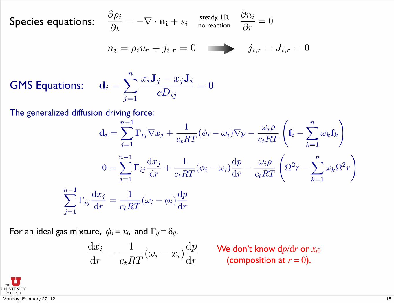
⇥�i
⇥t= �⇥ · ni + si
�ni
�r= 0
ni = �ivr + ji,r = 0 ji,r = Ji,r = 0
Species equations:
GMS Equations:
The generalized diffusion driving force:
di =n�1X
j=1
�ijrxj +1
ctRT(⇥i � ⇤i)rp� ⇤i�
ctRT
fi �
nX
k=1
⇤kfk
!
di =nX
j=1
xiJj � xjJi
cDij= 0
steady, 1D, no reaction
For an ideal gas mixture, φi = xi, and Γij = δij.
We don’t know dp/dr or xi0 (composition at r = 0).
0 =n�1X
j=1
�ijdxj
dr+
1
ctRT(⇥i � ⇤i)
dp
dr� ⇤i�
ctRT
⇥2r �
nX
k=1
⇤k⇥2r
!
n�1X
j=1
�ijdxj
dr=
1
ctRT(⇤i � ⇥i)
dp
dr
dxi
dr=
1
ctRT(�i � xi)
dp
dr
15Monday, February 27, 12

For species i,
Species mole balance:
Z rL
0p xi r dr = p
⇤x
⇤ir
2L
2Must know p(r) and
xi(r) to integrate this.
Momentum:
at steady state (no flow):
dp
dr= �
nX
i=1
⇥ifr,i = ��2r
⇤�v⇤t
= �⇥ · (�vv)�⇥ · ⌧ �⇥p + �nX
i=1
⇥ifi
We don’t know p0(pressure at r = 0).
Species mole balance constrains the species profile solution(dictates the species boundary condition)
The momentum equation gives the pressure profile,
but is coupled to the species equations through M.dp
dr= ��2r =
pM
RT�2r
Z rL
0cxi2�r dr =
Z rL
0c⇤x⇤
i 2�r dr
dxi
dr=
1
ctRT(�i � xi)
dp
dr
* indicates the initial condition (pure stream).
16Monday, February 27, 12

* indicates the initial condition (pure stream).
c =p
RT
Total mole balance (at equilibrium):
Substitute p(r) and solve this for p0...
Z
VcdV =
Z
Vc⇤ dV
Z rL
0cr dr = c⇤
r2L
2Z rL
0pr dr = p⇤
r2L
2
dV = L2�rdr
Total mole balance constrains the pressure solution(dictates the pressure boundary condition)
dxi
dr=
M
RT(�i � xi)�2rSolve these
equations:
With these constraints:
Z rL
0pr dr = p⇤
r2L
2
Z rL
0p xi r dr = p
⇤x
⇤ir
2L
2
Option A:1. Guess xi0, p0.2. Numerically solve the ODEs for xi, p.3. Are the constraints met? If not,
return to step 1.
Option B:Try to simplify the problem by making approximations.
dp
dr= ��2r =
pM
RT�2r Note: M couples all of the
equations together and makes them nonlinear.
Note: for tips on solving ODEs numerically in Matlab, see my wiki page.17Monday, February 27, 12

Approximation Level 1• Approximate M as constant, (MO2+MN2)/2, for
the pressure equation only. This decouples the pressure solution from the species and gives an easy analytic solution for pressure profile.
• Solve species equations numerically, given the analytic pressure profile.
Example: separation of Air into N2, O2.
Approximation Level 2• Approximate M as constant,
(MO2+MN2)/2, for the species and pressure equations.
• Obtain a fully analytic solution for both species and pressure.
• Centrifuge diameter: 20 cm • Air initially at STP
0 0.02 0.04 0.06 0.08 0.10
0.05
0.1
0.15
0.2
0.25
r (m)
O2 M
ole
Frac
tion
numericapproximate 1approximate 2
1,000 RPM
50,000 RPM
100,000 RPM
500,000 RPM
0 0.02 0.04 0.06 0.08 0.1
1e−4
1e−2
1
1e1
r (m)
p (a
tm)
fully numericconstant M
50,000 RPM
1000 RPM
100,000 RPM
150,000 RPM
18Monday, February 27, 12

Fick’s Law (revisited)
Ignoring thermal diffusion,
How do we interpret each term?When is each term important?
Notes: [D]=[B]-1[Γ]
In the binary case: D11=Γ11Ð12
For ideal mixtures: [Γ]=[I]
di = �n⇤
j=1
xixj
⇥Dij
�ji⇤i� jj
⇤j
⇥�⇥ lnT
n⇤
j=1
xixj�Tij
= �n⇤
j=1
xjJi � xiJj
cDij�⇥ lnT
n⇤
j=1
xixj�Tij J = �c[B]�1(d)�⇥ lnT (DT )
This is the same [B] matrix as before (T&K eq. 2.1.21-2.1.22)
di =n�1⇤
j=1
�ij⇥xj +1
ctRT(⇥i � ⇤i)⇥p� �i
ctRT
�fi �
n⇤
k=1
⇤kfk
⇥
(J) = �c[B]�1[�](⇥x)⇤ ⇥� ⌅1
� ⇥p
RT[B]�1 ((⇥)� (⇤))
⇤ ⇥� ⌅2
� �
RT[B]�1[⇤] ((f)� [⇤](f + fn))
⇤ ⇥� ⌅3
19Monday, February 27, 12

Review:Where we are, where we’re going…Accomplishments• Defined “reference velocities” and
“diffusion fluxes”
• Governing equations for multicomponent, reacting flow.‣mass-averaged velocity…
• Established a rigorous way to compute the diffusive fluxes from first principles.‣Can handle diffusion in systems of
arbitrary complexity, including:‣ nonideal mixtures, EM fields, large pressure
& temperature gradients, multiple species, chemical reaction, etc.
• Simplifications for ideal mixtures, negligible pressure gradients, etc.
• Solutions for “simple” problems.
Still Missing:• Models for binary diffusivities.‣Given a model, we are good to go!
Roadmap:• Models for binary diffusivities.
(T&K Chapter 4) - we won’t cover this...
• Simplified models for multicomponent diffusion
• Interphase mass transfer (surface discontinuities)
• Turbulence - models for diffusion in turbulent flow.
• Combined heat, mass, momentum transfer.
20Monday, February 27, 12
Recommended