GMM ESTIMATION OF ASSET PRICINGMODELS
Patrick GAGLIARDINIUniversity of Lugano and Swiss Finance Institute
Patrick Gagliardini (USI and SFI) GMM Estimation of asset pricing models 1 / 40

Outline
1 Rational expectations and no-arbitrage pricing models
2 Empirical analysis with GMM
3 Weak identification
4 Inference robust to weak identification
5 GMM with optimal instruments
6 Information-theoretic GMM
7 Lack of identification in asset pricing models
8 XMM and efficient derivative pricing
Patrick Gagliardini (USI and SFI) GMM Estimation of asset pricing models 2 / 40
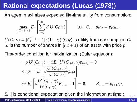
Rational expectations (Lucas (1978))An agent maximizes expected life-time utility from consumption:
max{Ct},{αt}
E0
[ ∞∑t=0
βtU(Ct; γ)
]s.t. Ct + ptαt = ptαt−1
U(Ct; γ) = [C1−γt − 1]/(1 − γ) (say) is utility from consumption Ct
αt is the number of shares in [t, t + 1) of an asset with price pt
First-order condition for maximization (Euler equation):
−ptU′(Ct; γ) + βEt [U
′(Ct+1; γ)pt+1] = 0
⇔ pt = Et
[β
U′(Ct+1; γ)
U′(Ct; γ)pt+1
]⇔ Et
[β
U′(Ct+1; γ)
U′(Ct; γ)Rt+1 − 1
]= 0, Rt+1 = pt+1/pt
Et[.] is conditional expectation given the information at time tPatrick Gagliardini (USI and SFI) GMM Estimation of asset pricing models 3 / 40
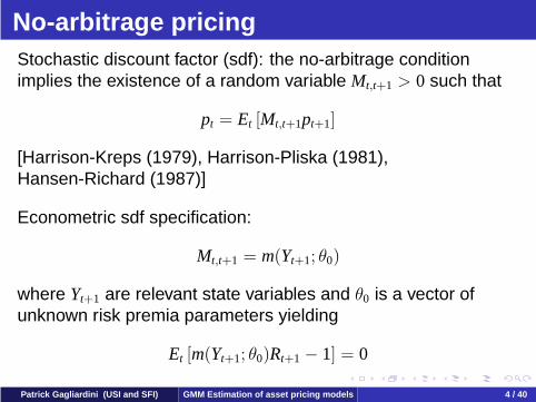
No-arbitrage pricingStochastic discount factor (sdf): the no-arbitrage conditionimplies the existence of a random variable Mt,t+1 > 0 such that
pt = Et [Mt,t+1pt+1]
[Harrison-Kreps (1979), Harrison-Pliska (1981),Hansen-Richard (1987)]
Econometric sdf specification:
Mt,t+1 = m(Yt+1; θ0)
where Yt+1 are relevant state variables and θ0 is a vector ofunknown risk premia parameters yielding
Et [m(Yt+1; θ0)Rt+1 − 1] = 0
Patrick Gagliardini (USI and SFI) GMM Estimation of asset pricing models 4 / 40
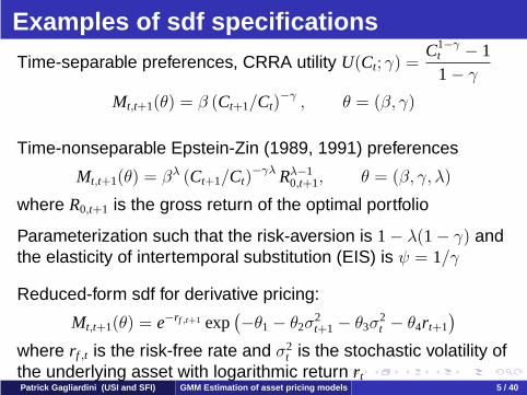
Examples of sdf specifications
Time-separable preferences, CRRA utility U(Ct; γ) =C1−γ
t − 11 − γ
Mt,t+1(θ) = β (Ct+1/Ct)−γ , θ = (β, γ)
Time-nonseparable Epstein-Zin (1989, 1991) preferences
Mt,t+1(θ) = βλ (Ct+1/Ct)−γλ Rλ−1
0,t+1, θ = (β, γ, λ)
where R0,t+1 is the gross return of the optimal portfolio
Parameterization such that the risk-aversion is 1 − λ(1 − γ) andthe elasticity of intertemporal substitution (EIS) is ψ = 1/γ
Reduced-form sdf for derivative pricing:
Mt,t+1(θ) = e−rf ,t+1 exp(−θ1 − θ2σ
2t+1 − θ3σ
2t − θ4rt+1
)where rf ,t is the risk-free rate and σ2
t is the stochastic volatility ofthe underlying asset with logarithmic return rtPatrick Gagliardini (USI and SFI) GMM Estimation of asset pricing models 5 / 40

Conditional moment restrictions
Let the information at date t be contained in the stochastic vectorWt following a Markov process, e.g. Wt = (Yt,Yt−1, · · · ,Yt−q)
Euler conditions/no-arbitrage conditions yield restrictions ondata and parameters in the form of a ...
Conditional Moment Restriction (CMR):
E [h(Yt+1; θ0)|Wt] = 0
where
h(Yt+1; θ) = m(Yt+1; θ)Rt+1 − 1
Patrick Gagliardini (USI and SFI) GMM Estimation of asset pricing models 6 / 40

From conditional to unconditional MR
Let Zt = ϕ(Wt) be an instrument
By the iterated expectation theorem:
E [Zth(Yt+1; θ0)] = E [E [Zth(Yt+1; θ0)|Wt]]
= E [ZtE [h(Yt+1; θ0)|Wt]]
= 0
which yields an ...
Unconditional Moment Restriction (UMR):
E [g(Xt; θ0)] = 0
where g(Xt; θ0) = Zth(Yt+1θ0)
Patrick Gagliardini (USI and SFI) GMM Estimation of asset pricing models 7 / 40
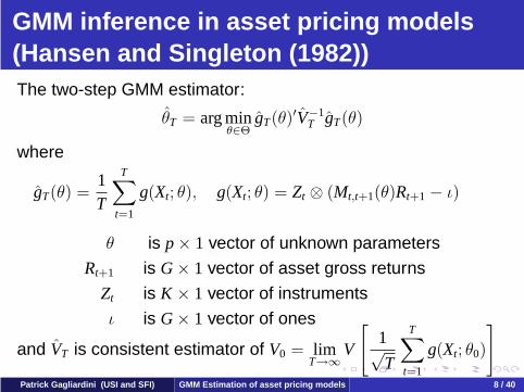
GMM inference in asset pricing models(Hansen and Singleton (1982))The two-step GMM estimator:
θT = arg minθ∈Θ
gT(θ)′V−1T gT(θ)
where
gT(θ) =1T
T∑t=1
g(Xt; θ), g(Xt; θ) = Zt ⊗ (Mt,t+1(θ)Rt+1 − ι)
θ is p × 1 vector of unknown parameters
Rt+1 is G × 1 vector of asset gross returns
Zt is K × 1 vector of instruments
ι is G × 1 vector of ones
and VT is consistent estimator of V0 = limT→∞
V
[1√T
T∑t=1
g(Xt; θ0)
]Patrick Gagliardini (USI and SFI) GMM Estimation of asset pricing models 8 / 40
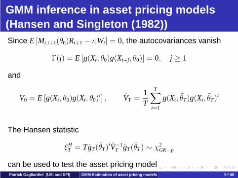
GMM inference in asset pricing models(Hansen and Singleton (1982))Since E [Mt,t+1(θ0)Rt+1 − ι|Wt] = 0, the autocovariances vanish
Γ(j) = E [g(Xt, θ0)g(Xt+j, θ0)] = 0, j ≥ 1
and
V0 = E [g(Xt, θ0)g(Xt, θ0)′] , VT =
1T
T∑t=1
g(Xt, θT)g(Xt, θT)′
The Hansen statistic
ξHT = TgT(θT)′V−1
T gT(θT) ∼ χ2GK−p
can be used to test the asset pricing modelPatrick Gagliardini (USI and SFI) GMM Estimation of asset pricing models 9 / 40
Empirical results:Hansen and Singleton (1982)Monthly data from 1959:2 to 1977:12
Returns of equally-weighted and value-weighted portfolios ofNYSE stocks
Instruments include current and lagged values of asset returnand consumption growth
Time-separable preferences, CRRA utility U(C; γ) =C1−γ − 1
1 − γ
Estimates of risk-aversion γ range between 0.5 and 1 withstandard errors of about 0.20
Hansen overidentification test rejects the modelPatrick Gagliardini (USI and SFI) GMM Estimation of asset pricing models 10 / 40
Empirical results: Stock and Wright (2000)
Monthly data on stock and bond portfolios from 1959:1 to1990:12
Instruments include additionally current and lagged values ofbond term spread and dividend yield
CRRA utility: estimated risk-aversion between 0 and 1
Epstein-Zin preferences: estimated risk-aversion is oftennegative!
Patrick Gagliardini (USI and SFI) GMM Estimation of asset pricing models 11 / 40
Empirical results: Yogo (2004)Yogo (2004) estimates the EIS ψ by GMM from the regression
Δct+1 = α+ ψrf ,t+1 + εt+1
where Δct+1 = log(Ct+1/Ct) is log consumption growth
For time-separable preferences and CRRA utility ψ = 1/γ
The CMR E [Δct+1 − α− ψrf ,t+1|Wt] = 0 corresponds to thelinearized Euler condition with CRRA utility written for theriskfree asset and divided by γ
GMM estimates of EIS ψ are in general small (and sometimesnegative!), in accordance with Hall (1988)
Results suggest that risk-aversion γ =1ψ
is (much) larger than 1
Patrick Gagliardini (USI and SFI) GMM Estimation of asset pricing models 12 / 40
Empirical results: Hall (2005)
Monthly stock returns data as in Hansen and Singleton (1982)but on the period 1959:1-1997:12
Instruments include current and past values of asset return andconsumption growth only
Time-separable preferences with CRRA utility
Estimated risk-aversion ranges between 0.7 and 1.3
Confidence intervals for γ are large, e.g. (−4, 4)
Patrick Gagliardini (USI and SFI) GMM Estimation of asset pricing models 13 / 40

Summary on empirical analysisAdvantage of GMM:
allows to estimate general nonlinear rational expectations andno-arbitrage asset pricing models “when only a subset of theeconomic environment is explicitly specified a-priori”
Drawbacks of GMM:
Instability of estimates when changing basic asset returnsand/or instruments and/or parameterization
Large confidence intervals for some preference parameterssuch as risk-aversion coefficient
Confidence intervals and hypothesis tests based on standardasymptotic approximations are often unreliable in finite sample[see e.g. Hansen, Heaton, Yaron (1996)]Patrick Gagliardini (USI and SFI) GMM Estimation of asset pricing models 14 / 40

Weak identification
Drawbacks of GMM are likely related to weak identification
A parameter θ is weakly identified when the UMR is not veryinformative to estimate the true value θ0
Figures 3.1 and 3.2 in Hall (2005), pp. 62 and 64, show that theGMM criterion is very flat over a wide range of values of therisk-aversion parameter!
Locally, weak identification means that the Jacobian matrix
J0 = E0
[∂g(Xt; θ0)
∂θ′
]= E0
[Zt∂Mt,t+1(θ0)
∂θ′
]is near reduced-rank, i.e., the instrument Zt is only weaklycorrelated with (some function of) the future state variables
Patrick Gagliardini (USI and SFI) GMM Estimation of asset pricing models 15 / 40
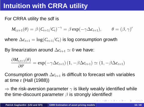
Intuition with CRRA utility
For CRRA utility the sdf is
Mt,t+1(θ) = β (Ct+1/Ct)−γ = β exp(−γΔct+1), θ = (β, γ)′
where Δct+1 = log(Ct+1/Ct) is log consumption growth
By linearization around Δct+1 � 0 we have:
∂Mt,t+1(θ)
∂θ′= exp(−γΔct+1) (1,−βΔct+1) � (1,−βΔct+1)
Consumption growth Δct+1 is difficult to forecast with variablesat time t (Hall (1988))
⇒ the risk-aversion parameter γ is likely weakly identified whilethe time-discount parameter β is strongly identified!
Patrick Gagliardini (USI and SFI) GMM Estimation of asset pricing models 16 / 40
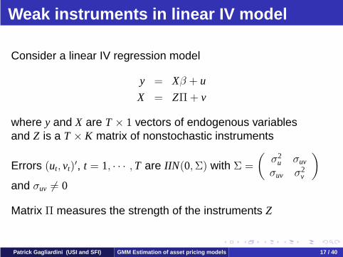
Weak instruments in linear IV model
Consider a linear IV regression model
y = Xβ + u
X = ZΠ + v
where y and X are T × 1 vectors of endogenous variablesand Z is a T × K matrix of nonstochastic instruments
Errors (ut, vt)′, t = 1, · · · ,T are IIN(0,Σ) with Σ =
(σ2
u σuv
σuv σ2v
)and σuv = 0
Matrix Π measures the strength of the instruments Z
Patrick Gagliardini (USI and SFI) GMM Estimation of asset pricing models 17 / 40
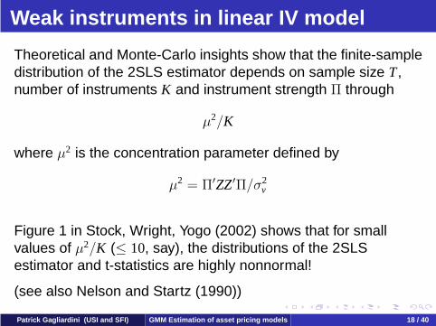
Weak instruments in linear IV model
Theoretical and Monte-Carlo insights show that the finite-sampledistribution of the 2SLS estimator depends on sample size T,number of instruments K and instrument strength Π through
μ2/K
where μ2 is the concentration parameter defined by
μ2 = Π′ZZ′Π/σ2v
Figure 1 in Stock, Wright, Yogo (2002) shows that for smallvalues of μ2/K (≤ 10, say), the distributions of the 2SLSestimator and t-statistics are highly nonnormal!
(see also Nelson and Startz (1990))
Patrick Gagliardini (USI and SFI) GMM Estimation of asset pricing models 18 / 40
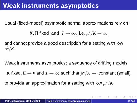
Weak instruments asymptotics
Usual (fixed-model) asymptotic normal approximations rely on
K,Π fixed and T → ∞, i.e. μ2/K → ∞
and cannot provide a good description for a setting with lowμ2/K !
Weak instruments asymptotics: a sequence of drifting models
K fixed,Π → 0 and T → ∞ such that μ2/K → constant (small)
to provide an approximation for a setting with low μ2/K
Patrick Gagliardini (USI and SFI) GMM Estimation of asset pricing models 19 / 40
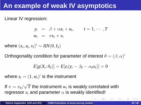
An example of weak IV asymptotics
Linear IV regression:
yt = β + αxt + ut, t = 1, · · · ,Twt = πxt + vt
where (xt, ut, vt)′ ∼ IIN(0, I3)
Orthogonality condition for parameter of interest θ = (β, α)′
E[g(Xt; θ0)] = E[zt(yt − β0 − α0xt)] = 0
where zt = (1,wt)′ is the instrument
If π = π0/√
T the instrument wt is weakly correlated withregressor xt and parameter α is weakly identified!
Patrick Gagliardini (USI and SFI) GMM Estimation of asset pricing models 20 / 40

An example of weak IV asymptoticsWrite the GMM=2SLS estimator as:
αT =
(T∑
t=1
(wt − w)(xt − x)
)−1 T∑t=1
(wt − w)yt, βT = y − xαT
Then:
αT − α0 =
(1√T
T∑t=1
(wt − w)(xt − x)
)−11√T
T∑t=1
(wt − w)utd→ Z1
π0 + Z2
√T(βT − β0
)=
√Tu −
√Tx (αT − α0)
d→ Z3 − Z1Z4
π0 + Z2
where (Z1,Z2,Z3,Z4)′ ∼ N(0, I4)
The estimator of the weakly identified parameter α isinconsistent while the estimator of the strongly identifiedparameter β is root-T consistent but asymptotically nonnormal!Patrick Gagliardini (USI and SFI) GMM Estimation of asset pricing models 21 / 40
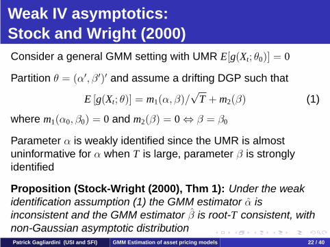
Weak IV asymptotics:Stock and Wright (2000)Consider a general GMM setting with UMR E[g(Xt; θ0)] = 0
Partition θ = (α′, β′)′ and assume a drifting DGP such that
E [g(Xt; θ)] = m1(α, β)/√
T + m2(β) (1)
where m1(α0, β0) = 0 and m2(β) = 0 ⇔ β = β0
Parameter α is weakly identified since the UMR is almostuninformative for α when T is large, parameter β is stronglyidentified
Proposition (Stock-Wright (2000), Thm 1): Under the weakidentification assumption (1) the GMM estimator α isinconsistent and the GMM estimator β is root-T consistent, withnon-Gaussian asymptotic distributionPatrick Gagliardini (USI and SFI) GMM Estimation of asset pricing models 22 / 40
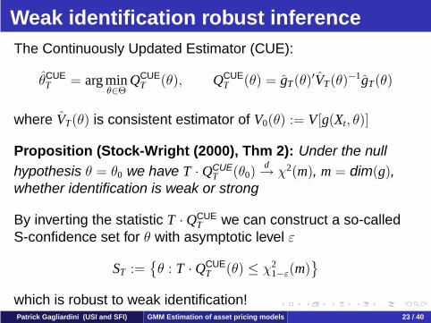
Weak identification robust inferenceThe Continuously Updated Estimator (CUE):
θCUET = arg min
θ∈ΘQCUE
T (θ), QCUET (θ) = gT(θ)′VT(θ)−1gT(θ)
where VT(θ) is consistent estimator of V0(θ) := V[g(Xt, θ)]
Proposition (Stock-Wright (2000), Thm 2): Under the nullhypothesis θ = θ0 we have T · QCUE
T (θ0)d→ χ2(m), m = dim(g),
whether identification is weak or strong
By inverting the statistic T · QCUET we can construct a so-called
S-confidence set for θ with asymptotic level ε
ST :={θ : T · QCUE
T (θ) ≤ χ21−ε(m)
}which is robust to weak identification!Patrick Gagliardini (USI and SFI) GMM Estimation of asset pricing models 23 / 40
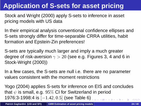
Application of S-sets for asset pricingStock and Wright (2000) apply S-sets to inference in assetpricing models with US data
In their empirical analysis conventional confidence ellipses andS-sets strongly differ for time-separable CRRA utilities, habitformation and Epstein-Zin preferences!
S-sets are typically much larger and imply a much greaterdegree of risk-aversion γ > 20 (see e.g. Figures 3, 4 and 6 inStock-Wright (2000))
In a few cases, the S-sets are null i.e. there are no parametervalues consistent with the moment restrictions
Yogo (2004) applies S-sets for inference on EIS and concludesthat ψ is small, e.g. 95% CI for Switzerland in period1976:3-1998:4 is [−1.42, 0.5] (see Table 6)Patrick Gagliardini (USI and SFI) GMM Estimation of asset pricing models 24 / 40
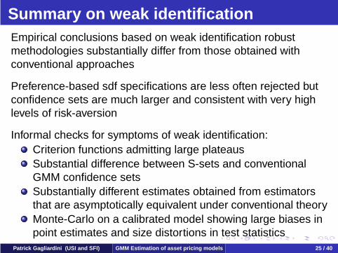
Summary on weak identificationEmpirical conclusions based on weak identification robustmethodologies substantially differ from those obtained withconventional approaches
Preference-based sdf specifications are less often rejected butconfidence sets are much larger and consistent with very highlevels of risk-aversion
Informal checks for symptoms of weak identification:Criterion functions admitting large plateausSubstantial difference between S-sets and conventionalGMM confidence setsSubstantially different estimates obtained from estimatorsthat are asymptotically equivalent under conventional theoryMonte-Carlo on a calibrated model showing large biases inpoint estimates and size distortions in test statistics
Patrick Gagliardini (USI and SFI) GMM Estimation of asset pricing models 25 / 40
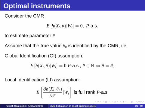
Optimal instrumentsConsider the CMR
E [h(Xt, θ)|Wt] = 0, P-a.s.
to estimate parameter θ
Assume that the true value θ0 is identified by the CMR, i.e.
Global Identification (GI) assumption:
E [h(Xt, θ)|Wt] = 0 P-a.s., θ ∈ Θ ⇔ θ = θ0
Local Identification (LI) assumption:
E
[∂h(Xt, θ0)
∂θ′|Wt
]is full rank P-a.s.
Patrick Gagliardini (USI and SFI) GMM Estimation of asset pricing models 26 / 40
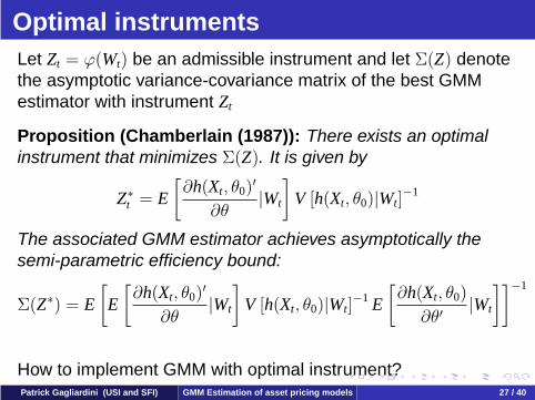
Optimal instrumentsLet Zt = ϕ(Wt) be an admissible instrument and let Σ(Z) denotethe asymptotic variance-covariance matrix of the best GMMestimator with instrument Zt
Proposition (Chamberlain (1987)): There exists an optimalinstrument that minimizes Σ(Z). It is given by
Z∗t = E
[∂h(Xt, θ0)
′
∂θ|Wt
]V [h(Xt, θ0)|Wt]
−1
The associated GMM estimator achieves asymptotically thesemi-parametric efficiency bound:
Σ(Z∗) = E
[E
[∂h(Xt, θ0)
′
∂θ|Wt
]V [h(Xt, θ0)|Wt]
−1 E
[∂h(Xt, θ0)
∂θ′|Wt
]]−1
How to implement GMM with optimal instrument?Patrick Gagliardini (USI and SFI) GMM Estimation of asset pricing models 27 / 40
Information-theoretic GMM
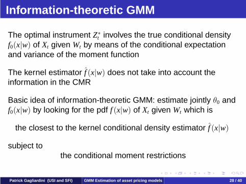
The optimal instrument Z∗t involves the true conditional density
f0(x|w) of Xt given Wt by means of the conditional expectationand variance of the moment function
The kernel estimator f (x|w) does not take into account theinformation in the CMR
Basic idea of information-theoretic GMM: estimate jointly θ0 andf0(x|w) by looking for the pdf f (x|w) of Xt given Wt which is
the closest to the kernel conditional density estimator f (x|w)
subject tothe conditional moment restrictions
Patrick Gagliardini (USI and SFI) GMM Estimation of asset pricing models 28 / 40
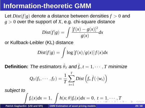
Information-theoretic GMMLet Dist(f |g) denote a distance between densities f > 0 andg > 0 over the support of X, e.g. chi-square distance
Dist(f |g) =
∫[f (x) − g(x)]2
g(x)dx
or Kullback-Leibler (KL) distance
Dist(f |g) =
∫log [f (x)/g(x)] f (x)dx
Definition: The estimators θT and ft, t = 1, · · · ,T minimize
QT(f1, · · · , fT) =1T
T∑t=1
Dist(
ft, f (·|wt))
subject to∫ft(x)dx = 1,
∫h(x; θ)ft(x)dx = 0, t = 1, · · · ,T
Patrick Gagliardini (USI and SFI) GMM Estimation of asset pricing models 29 / 40
Euclidean likelihood: Chi-square distance
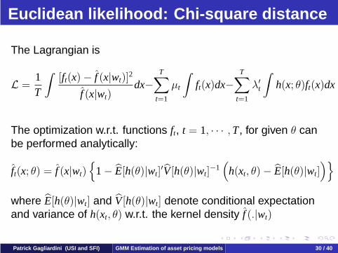
The Lagrangian is
L =1T
∫[ft(x) − f (x|wt)]
2
f (x|wt)dx−
T∑t=1
μt
∫ft(x)dx−
T∑t=1
λ′t
∫h(x; θ)ft(x)dx
The optimization w.r.t. functions ft, t = 1, · · · ,T, for given θ canbe performed analytically:
ft(x; θ) = f (x|wt){
1 − E[h(θ)|wt]′V[h(θ)|wt]
−1(
h(xt, θ) − E[h(θ)|wt])}
where E[h(θ)|wt] and V[h(θ)|wt] denote conditional expectationand variance of h(xt, θ) w.r.t. the kernel density f (.|wt)
Patrick Gagliardini (USI and SFI) GMM Estimation of asset pricing models 30 / 40
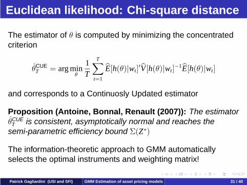
Euclidean likelihood: Chi-square distance
The estimator of θ is computed by minimizing the concentratedcriterion
θCUET = arg min
θ
1T
T∑t=1
E[h(θ)|wt]′V[h(θ)|wt]
−1E[h(θ)|wt]
and corresponds to a Continuosly Updated estimator
Proposition (Antoine, Bonnal, Renault (2007)): The estimatorθCUE
T is consistent, asymptotically normal and reaches thesemi-parametric efficiency bound Σ(Z∗)
The information-theoretic approach to GMM automaticallyselects the optimal instruments and weighting matrix!
Patrick Gagliardini (USI and SFI) GMM Estimation of asset pricing models 31 / 40

Exponential tilting: KL distanceThe estimates of ft, t = 1, · · · ,T, for given θ are
ft(x; θ) = f (x|wt) exp (λt(θ)′h(xt, θ)) /E [exp (λt(θ)
′h(xt, θ)) |wt]
where the Lagrange multiplier vector λt(θ) is such that the tilteddensity ft(x; θ) satisfies
∫h(x, θ)ft(x, θ)dx = 0
The exponential tilting (ET) estimator is
θETT = arg min
θ− 1
T
T∑t=1
log E [exp (λt(θ)′h(xt, θ)) |wt]
Proposition (Kitamura, Tripathi, Ahn (2004)): The ETestimator is asymptotically equivalent to CUE, in particularsemi-parametrically efficient
Computation of ET estimator is more cumbersome than CUEbut ensures positive estimated densities!Patrick Gagliardini (USI and SFI) GMM Estimation of asset pricing models 32 / 40
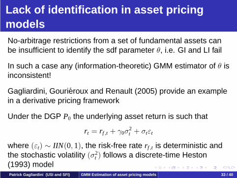
Lack of identification in asset pricingmodelsNo-arbitrage restrictions from a set of fundamental assets canbe insufficient to identify the sdf parameter θ, i.e. GI and LI fail
In such a case any (information-theoretic) GMM estimator of θ isinconsistent!
Gagliardini, Gourieroux and Renault (2005) provide an examplein a derivative pricing framework
Under the DGP P0 the underlying asset return is such that
rt = rf ,t + γ0σ2t + σtεt
where (εt) ∼ IIN(0, 1), the risk-free rate rf ,t is deterministic andthe stochastic volatility (σ2
t ) follows a discrete-time Heston(1993) modelPatrick Gagliardini (USI and SFI) GMM Estimation of asset pricing models 33 / 40
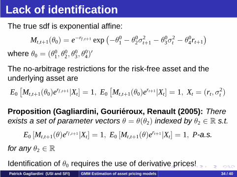
Lack of identificationThe true sdf is exponential affine:
Mt,t+1(θ0) = e−rf ,t+1 exp(−θ0
1 − θ02σ
2t+1 − θ0
3σ2t − θ0
4rt+1
)where θ0 = (θ0
1, θ02, θ
03, θ
04)
′
The no-arbitrage restrictions for the risk-free asset and theunderlying asset are
E0
[Mt,t+1(θ0)e
rf ,t+1|Xt] = 1, E0
[Mt,t+1(θ0)e
rt+1 |Xt] = 1, Xt = (rt, σ2t )
Proposition (Gagliardini, Gourieroux, Renault (2005): Thereexists a set of parameter vectors θ = θ(θ2) indexed by θ2 ∈ R s.t.
E0 [Mt,t+1(θ)erf ,t+1 |Xt] = 1, E0 [Mt,t+1(θ)e
rt+1 |Xt] = 1, P-a.s.
for any θ2 ∈ R
Identification of θ0 requires the use of derivative prices!Patrick Gagliardini (USI and SFI) GMM Estimation of asset pricing models 34 / 40
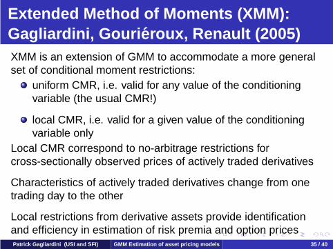
Extended Method of Moments (XMM):Gagliardini, Gourieroux, Renault (2005)XMM is an extension of GMM to accommodate a more generalset of conditional moment restrictions:
uniform CMR, i.e. valid for any value of the conditioningvariable (the usual CMR!)
local CMR, i.e. valid for a given value of the conditioningvariable only
Local CMR correspond to no-arbitrage restrictions forcross-sectionally observed prices of actively traded derivatives
Characteristics of actively traded derivatives change from onetrading day to the other
Local restrictions from derivative assets provide identificationand efficiency in estimation of risk premia and option pricesPatrick Gagliardini (USI and SFI) GMM Estimation of asset pricing models 35 / 40
ReferencesAntoine, B., Bonnal, H. and E. Renault (2007): “On the EfficientUse of the Informational Content of Estimating Equations:Implied Probabilities and Euclidean Empirical Likelihood”,Journal of Econometrics, 138, 461-487
Chamberlain, G. (1987): ”Asymptotic Efficiency in Estimationwith Conditional Moment Restrictions”’, Journal ofEconometrics, 34, 305-334
Epstein, L. and S. Zin (1989): “Substitution, Risk-Aversion, andthe Temporal Behaviour of Consumption and Asset Returns: ATheoretical Framework”, Econometrica, 57, 937-969
Epstein, L. and S. Zin (1991): “Substitution, Risk-Aversion, andthe Temporal Behaviour of Consumption and Asset Returns: AnEmpirical Analysis”, Journal of Political Economy, 99, 263-286Patrick Gagliardini (USI and SFI) GMM Estimation of asset pricing models 36 / 40
ReferencesGagliardini, P., Gourieroux, C. and E. Renault (2005): “EfficientDerivative Pricing by the Extended Method of Moments“,Working Paper.
Hall, A. (2005): Generalized Method of Moments, OxfordUniversity Press
Hall, R. (1988): “Intertemporal Substitution in Consumption”,Journal of Political Economy, 96, 339-357
Hansen, L., Heaton, J. and A. Yaron (1996): “Finite SampleProperties of Some Alternative GMM Estimators”, Journal ofBusiness and Economic Statistics, 14, 262-280
Hansen, L. and K. Singleton (1982): “Generalized InstrumentalVariable Estimation of Nonlinear Rational Expectations Models”,Econometrica, 50, 1269-1286Patrick Gagliardini (USI and SFI) GMM Estimation of asset pricing models 37 / 40
References
Hansen, L. and S. Richard (1987): ”The Role of ConditioningInformation in Deducing Testable Restrictions Implied byDynamic Asset Pricing Models”, Econometrica, 55, 587-613
Harrison, J. and D. Kreps (1979): ”Martingales and Arbitrage inMultiperiod Securities Markets”, Journal of Economic Theory,20, 381-408
Harrison, M. and S. Pliska (1981): ”Martingales and StochasticIntegrals in the Theory of Continuous Trading”’, StochasticProcesses and Their Applications, 11, 215-260
Heston, S. (1993): ”A Closed Form Solution for Options withStochastic Volatility with Applications to Bond and CurrencyOptions”, Review of Financial Studies, 6, 327-343
Patrick Gagliardini (USI and SFI) GMM Estimation of asset pricing models 38 / 40

ReferencesKitamura, Y. (2007): ”Empirical Likelihood Methods inEconometrics: Theory and Practice” in Advances in Economicsand Econometrics, Theory and Applications: Ninth WorldCongress of the Econometric Society, Vol. 3, eds. Blundell, R.,Newey, W., and T., Persson, Cambridge University Press,174-237
Kitamura, Y. and M. Stutzer (1997): “An Information TheoreticAlternative to Generalized Method of Moments Estimation”,Econometrica, 65, 861-874
Kitamura, Y., Tripathi, G. and H. Ahn (2004): “EmpiricalLikelihood Based Inference in Conditional Moment RestrictionModels”, Econometrica, 72, 1667-1714
Lucas, R. (1978): ”Asset Prices in an Exchange Economy”,Econometrica, 46, 1429-1446Patrick Gagliardini (USI and SFI) GMM Estimation of asset pricing models 39 / 40
References
Nelson, C. and R. Startz (1990): “Some Further Results on theExact Small Sample Properties of the Instrumental VariableEstimator”, Econometrica, 58, 967-976
Stock, J. and J. Wright (2000): “GMM with Weak Identification”,Econometrica, 68, 1055-1096
Stock, J., Wright, J. and M. Yogo (2002): “A Survey of WeakInstruments and Weak Identification in Generalized Method ofMoments”, Journal of Business and Economic Statistics, 20,518-529
Yogo, M. (2004): “Estimating the Elasticity of IntertemporalSubstitution When Instruments are Weak”, Review ofEconomics and Statistics, 86, 797-810
Patrick Gagliardini (USI and SFI) GMM Estimation of asset pricing models 40 / 40
Recommended