HAL Id: hal-00575576https://hal.archives-ouvertes.fr/hal-00575576
Submitted on 10 Mar 2011
HAL is a multi-disciplinary open accessarchive for the deposit and dissemination of sci-entific research documents, whether they are pub-lished or not. The documents may come fromteaching and research institutions in France orabroad, or from public or private research centers.
L’archive ouverte pluridisciplinaire HAL, estdestinée au dépôt et à la diffusion de documentsscientifiques de niveau recherche, publiés ou non,émanant des établissements d’enseignement et derecherche français ou étrangers, des laboratoirespublics ou privés.
Geometrical tools for the description and control offunctional specifications at the conceptual design phase.
Guillaume Mandil, Philippe Serré, Moinet Mireille, Alain Desrochers
To cite this version:Guillaume Mandil, Philippe Serré, Moinet Mireille, Alain Desrochers. Geometrical tools for the de-scription and control of functional specifications at the conceptual design phase.. IJODIR, 2011, 5(1). <hal-00575576>
1
Geometrical tools for the description and control of functional specifications at the conceptual design phase.
Guillaume MANDIL1,2, Philippe SERRÉ2, Mireille MOINET2, Alain DESROCHERS1 1 Université de Sherbrooke, Département de génie mécanique, 2500 boulevard de l’université, Sherbrooke Québec, Canadα J1K 2R1 2 LISMMA – Supméca Paris 3 rue Fernand Hainaut F-93407 Saint-Ouen Cedex, France [email protected] RÉSUMÉ. Cet article présente un modèle géométrique à base de points et de segments de droites utilisé pour représenter des mécanismes dans les phases de préconception. Ce modèle est traduit sous forme mathématique par une matrice d’incidence qui représente la topologie et une matrice de Gram qui représente les informations métriques de l’objet. Il est ensuite indiqué comment assembler deux objets représentés par ce modèle. Enfin, un exemple permet de montrer l’intérêt de ce modèle pour réaliser le suivi d’une exigence géométrique au cours du cycle de vie du produit.
ABSTRACT. This paper presents a geometrical model that uses points and line segments to describe mechanisms at the early phases of the product design process. This model allows the description of an object with a topological matrix and another matrix that contains the metric information about the object. The paper also indicates how to associate two objects represented using this model. Finally, the interest of this model for the mapping of a geometrical requirement along the product life-cycle is shown on a case study.
MOTS-CLÉS : Exigence géométrique, Cycle de vie, Tenseur métrique, Matrices de Gram, Géométrie non Cartésiennes.
KEYWORDS: Geometrical requirement; Life Cycle; Metric tensor; Gram matrices; coordinate free geometry.
2
1. Introduction
During the design process of a mechanical product, functional requirements are translated into geometrical requirements. For instance the functional requirement saying that: “part A must follow a given face of part B along the movement” can be translated as: “The clearance between the two surfaces of part A and B must remain inferior to x mm”. This translation could also be applied to the definition of kinematic joints. The technique developed by M’Henni [M'henni, 2010] allows the accurate calculation of the geometrical parameters of the joint. Moreover, a mechanical product is subjected to dimensional variations along its life cycle due to mechanical strains. These variations affect the dimensions of parts that in turn influence the value of the geometrical requirements. Generally there exist several useful values of a requirement depending on the use-‐case or the user. For instance, the manufacturer is interested in the value of the geometrical requirements at the assembly stage of the life-‐cycle to perform the assembly of the parts and components. From another point of view, the final user is interested in the values of the same requirement but under operating conditions.
As a matter of fact, considering the designer’s point of view, it becomes necessary to link (or to compare) the values of a geometrical requirement at several stages of the product life-‐cycle. In particular, for the designer, several problems appear: “Does the chosen dimension for manufacturing (or assembly) allow the geometrical requirements under operating conditions to be met?” or “Which dimensions must be specified on the drawing to ensure a given value of the geometrical requirement in operation?”
In order to compare the geometric configuration of an object (or product) at two distinct stages of its life-‐cycle, this paper proposes a technique to combine the two mathematical representations of the same object under different use-‐cases in a unique and common representation.
Authors noticed that there exist various tools to manage the detailed design of a product. For instance the Computer Aided Design (CAD) tools help designers define the detailed and nominal 3D geometry of a product. From this nominal geometrical model it becomes possible to use a Finite Element Analysis (FEA) to calculate the dimension variations due to mechanical strains [Pierre et al., 2009] and to rebuild a geometrical model [Louhichi, 2008]. Form the nominal model, there also exists several methods [Ghie, 2004], [Anselmetti, 2006], to deal with the tolerancing problem. This addresses the issue of the real versus nominal dimensions of the parts. These methods help the mechanical designer in the specification of tolerances zones and the management and control of dimensional uncertainties due to manufacturing.
On the other hand, there are few tools available for geometry management at the early design phases. Consequently this work proposes a geometrical model dedicated to preliminary design that allows the calculation of the evolution of geometrical parameters or requirements along the product life-‐cycle. In consequence, this work includes the proposition of a simplified coordinate free representation to represent objects. Coordinate free approaches allow the direct specification of intrinsic properties of geometrical objects that avoid the artificial dependence with a reference frame induced by the coordinates.
3
The first part of this paper will detail the topological and vectorial model used for representing the object. Then the second part will detail how to associate two topological models. Finally, the third part of the paper will explicit the association of two vectorial models.
2. Notations
This paper will use the following conventions:
Matrices will be noted with capital bold letters: M ;
Vectors will be noted with bold letters: u ;
Scalar number will be noted with italic letters: x.
Scalar product of vectors u and v is noted <u,v>
⊗ represent the product of two matrices.
3. Models
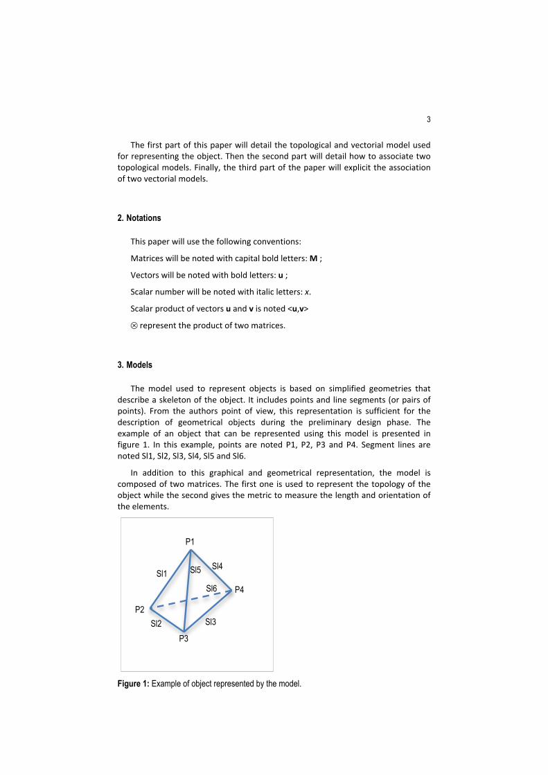
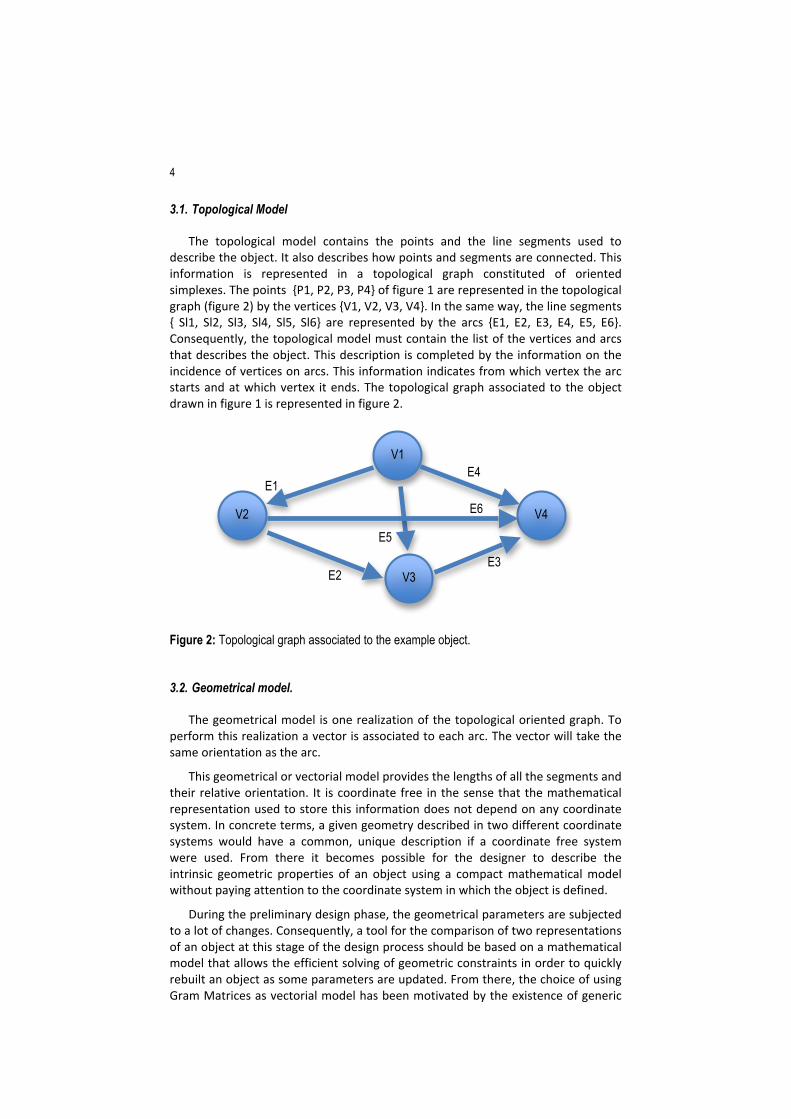
The model used to represent objects is based on simplified geometries that describe a skeleton of the object. It includes points and line segments (or pairs of points). From the authors point of view, this representation is sufficient for the description of geometrical objects during the preliminary design phase. The example of an object that can be represented using this model is presented in figure 1. In this example, points are noted P1, P2, P3 and P4. Segment lines are noted Sl1, Sl2, Sl3, Sl4, Sl5 and Sl6.
In addition to this graphical and geometrical representation, the model is composed of two matrices. The first one is used to represent the topology of the object while the second gives the metric to measure the length and orientation of the elements.
Figure 1: Example of object represented by the model.
P1
P2
P3
P4
Sl1
Sl2 Sl3
Sl4 Sl5
Sl6
4
3.1. Topological Model
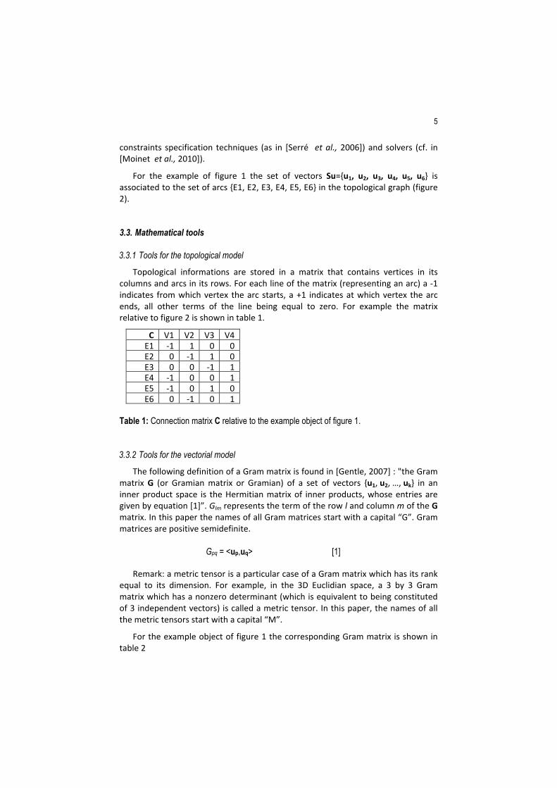
The topological model contains the points and the line segments used to describe the object. It also describes how points and segments are connected. This information is represented in a topological graph constituted of oriented simplexes. The points {P1, P2, P3, P4} of figure 1 are represented in the topological graph (figure 2) by the vertices {V1, V2, V3, V4}. In the same way, the line segments { Sl1, Sl2, Sl3, Sl4, Sl5, Sl6} are represented by the arcs {E1, E2, E3, E4, E5, E6}. Consequently, the topological model must contain the list of the vertices and arcs that describes the object. This description is completed by the information on the incidence of vertices on arcs. This information indicates from which vertex the arc starts and at which vertex it ends. The topological graph associated to the object drawn in figure 1 is represented in figure 2.
Figure 2: Topological graph associated to the example object.
3.2. Geometrical model.
The geometrical model is one realization of the topological oriented graph. To perform this realization a vector is associated to each arc. The vector will take the same orientation as the arc.
This geometrical or vectorial model provides the lengths of all the segments and their relative orientation. It is coordinate free in the sense that the mathematical representation used to store this information does not depend on any coordinate system. In concrete terms, a given geometry described in two different coordinate systems would have a common, unique description if a coordinate free system were used. From there it becomes possible for the designer to describe the intrinsic geometric properties of an object using a compact mathematical model without paying attention to the coordinate system in which the object is defined.
During the preliminary design phase, the geometrical parameters are subjected to a lot of changes. Consequently, a tool for the comparison of two representations of an object at this stage of the design process should be based on a mathematical model that allows the efficient solving of geometric constraints in order to quickly rebuilt an object as some parameters are updated. From there, the choice of using Gram Matrices as vectorial model has been motivated by the existence of generic
E4 E1
E2 E3
E5
E6
V3
V1
V2 V4
5 constraints specification techniques (as in [Serré et al., 2006]) and solvers (cf. in [Moinet et al., 2010]).
For the example of figure 1 the set of vectors Su={u1, u2, u3, u4, u5, u6} is associated to the set of arcs {E1, E2, E3, E4, E5, E6} in the topological graph (figure 2).
3.3. Mathematical tools
3.3.1 Tools for the topological model
Topological informations are stored in a matrix that contains vertices in its columns and arcs in its rows. For each line of the matrix (representing an arc) a -‐1 indicates from which vertex the arc starts, a +1 indicates at which vertex the arc ends, all other terms of the line being equal to zero. For example the matrix relative to figure 2 is shown in table 1.
C V1 V2 V3 V4 E1 -‐1 1 0 0 E2 0 -‐1 1 0 E3 0 0 -‐1 1 E4 -‐1 0 0 1 E5 -‐1 0 1 0 E6 0 -‐1 0 1
Table 1: Connection matrix C relative to the example object of figure 1.
3.3.2 Tools for the vectorial model
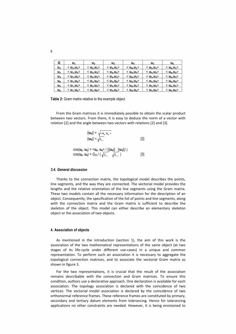
The following definition of a Gram matrix is found in [Gentle, 2007] : "the Gram matrix G (or Gramian matrix or Gramian) of a set of vectors {u1, u2, …, uk} in an inner product space is the Hermitian matrix of inner products, whose entries are given by equation [1]”. Glm represents the term of the row l and column m of the G matrix. In this paper the names of all Gram matrices start with a capital “G”. Gram matrices are positive semidefinite.
1 Gpq = <up,uq> [1]
Remark: a metric tensor is a particular case of a Gram matrix which has its rank equal to its dimension. For example, in the 3D Euclidian space, a 3 by 3 Gram matrix which has a nonzero determinant (which is equivalent to being constituted of 3 independent vectors) is called a metric tensor. In this paper, the names of all the metric tensors start with a capital “M”.
For the example object of figure 1 the corresponding Gram matrix is shown in table 2
6
G u1 u2 u3 u4 u5 u6 u1 < u1,u1> < u2,u1> < u3,u1> < u4,u1> < u5,u1> < u6,u1> u2 < u1,u2> < u2,u2> < u3,u2> < u4,u2> < u5,u2> < u6,u2> u3 < u1,u3> < u2,u3> < u3,u3> < u4,u3> < u5,u3> < u6,u3> u4 < u1,u4> < u2,u4> < u3,u4> < u4,u4> < u5,u4> < u6,u4> u5 < u1,u5> < u2,u5> < u3,u5> < u4,u5> < u5,u5> < u6,u5> u6 < u1,u6> < u2,u6> < u3,u6> < u4,u6> < u5,u6> < u6,u6>
Table 2: Gram matrix relative to the example object.
From the Gram matrices it is immediately possible to obtain the scalar product between two vectors. From there, it is easy to deduce the norm of a vector with relation [2] and the angle between two vectors with relations [2] and [3].
2 ||up|| =
||up|| = [2]
3 cos(up, uq) = <up, uq> / (||up|| ||uq||) ) cos(up, uq) = Gpq / ( ) [3]
3.4. General discussion
Thanks to the connection matrix, the topological model describes the points, line segments, and the way they are connected. The vectorial model provides the lengths and the relative orientation of the line segments using the Gram matrix. These two models contain all the necessary information for the description of an object. Consequently, the specification of the list of points and line segments, along with the connection matrix and the Gram matrix is sufficient to describe the skeleton of the object. This model can either describe an elementary skeleton object or the association of two objects.
4. Association of objects
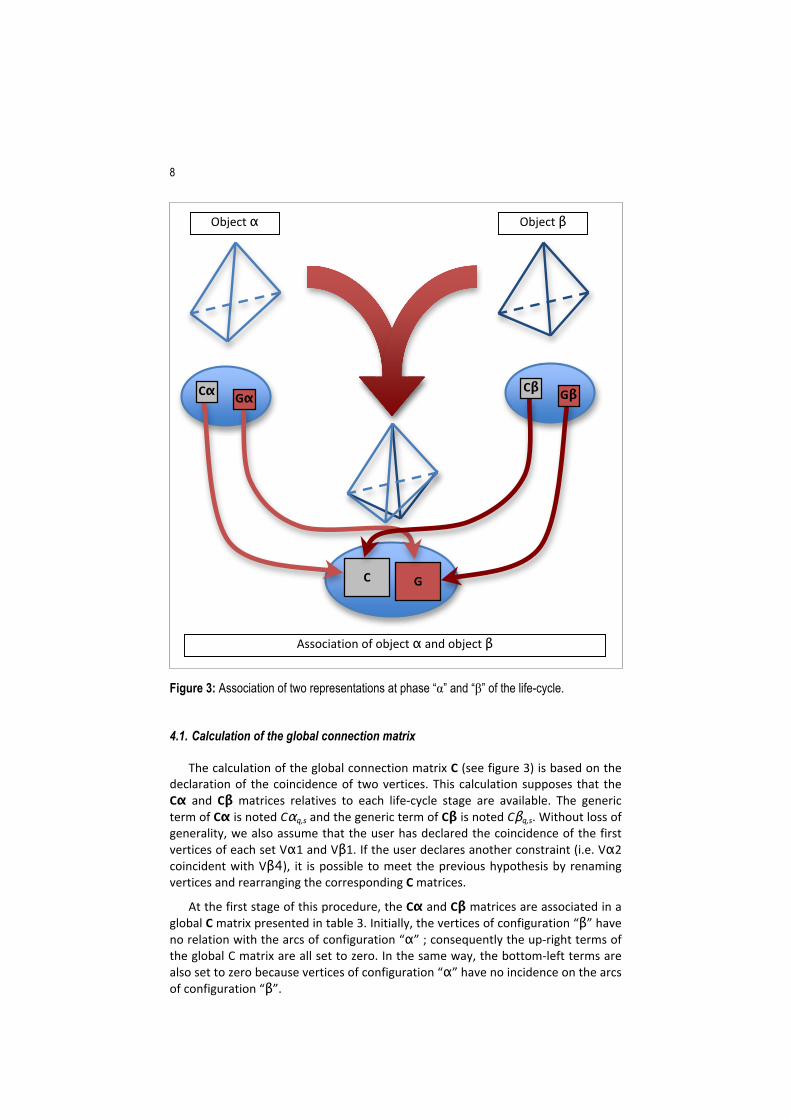
As mentioned in the introduction (section 1), the aim of this work is the association of the two mathematical representations of the same object (at two stages of its life-‐cycle under different use-‐cases) in a unique and common representation. To perform such an association it is necessary to aggregate the topological connection matrices, and to associate the vectorial Gram matrix as shown in figure 3.
For the two representations, it is crucial that the result of the association remains describable with the connection and Gram matrices. To ensure this condition, authors use a declarative approach. One declaration is available for each association. The topology association is declared with the coincidence of two vertices. The vectorial model association is declared by the coincidence of two orthonormal reference frames. These reference frames are constituted by primary, secondary and tertiary datum elements from tolerancing. Hence for tolerancing applications no other constraints are needed. However, it is being envisioned to
7 add other constraints for the declaration of the association of two objects to extend this approach to other fields of product design.
In any case, this paper considers that a complete representation of the elementary objects to be associated already exists, thanks to a connection matrix and a Gram matrix. For this application it is assumed that a model of the object exists. This model is instanced at two distinct stages “α” and “β” of the life-‐cycle. The reader is advised that the letters α and β always refer to the life cycle stages in all the following variable names. For the stage “α” of the life cycle two matrices are available : Gα and Cα. The elements of the Gα Gram matrix are scalar products between vectors from the set Suα = {uα1, uα2, …, uαq}. The Cα connection matrix indicates the relations between the arcs {Eα1, Eα2, … , Eαq} and the vertices {Vα1, Vα2, … , Vαs}. The index q is used to count arcs and vectors and the index s is used to count vertices. For the stage “β” of the life cycle, the matrix Gβ represents the set Suβ = {uβ1, uβ2, …, uβq} and the matrix Cβ indicates the connection between the arcs {Eβ1, Eβ2, … , Eβq} and the vertices {Vβ1, Vβ2, … , Vβs}.
In our case, there are no changes in the topology of the object; consequently Cα = Cβ. Moreover, at the stage “α” of the life cycle, the Cα and Gα matrices can be obtained with the technique developed by Moinet [Moinet, 2008]. The Cβ and Gβ matrices are calculated using the same approach.
8
Figure 3: Association of two representations at phase “α” and “β” of the life-cycle.
4.1. Calculation of the global connection matrix
The calculation of the global connection matrix C (see figure 3) is based on the declaration of the coincidence of two vertices. This calculation supposes that the Cα and Cβ matrices relatives to each life-‐cycle stage are available. The generic term of Cα is noted Cαq,s and the generic term of Cβ is noted Cβq,s. Without loss of generality, we also assume that the user has declared the coincidence of the first vertices of each set Vα1 and Vβ1. If the user declares another constraint (i.e. Vα2 coincident with Vβ4), it is possible to meet the previous hypothesis by renaming vertices and rearranging the corresponding C matrices.
At the first stage of this procedure, the Cα and Cβ matrices are associated in a global C matrix presented in table 3. Initially, the vertices of configuration “β” have no relation with the arcs of configuration “α” ; consequently the up-‐right terms of the global C matrix are all set to zero. In the same way, the bottom-‐left terms are also set to zero because vertices of configuration “α” have no incidence on the arcs of configuration “β”.
Object α
C G
Association of object α and object β
Object β
Cα Gα Cβ Gβ
9
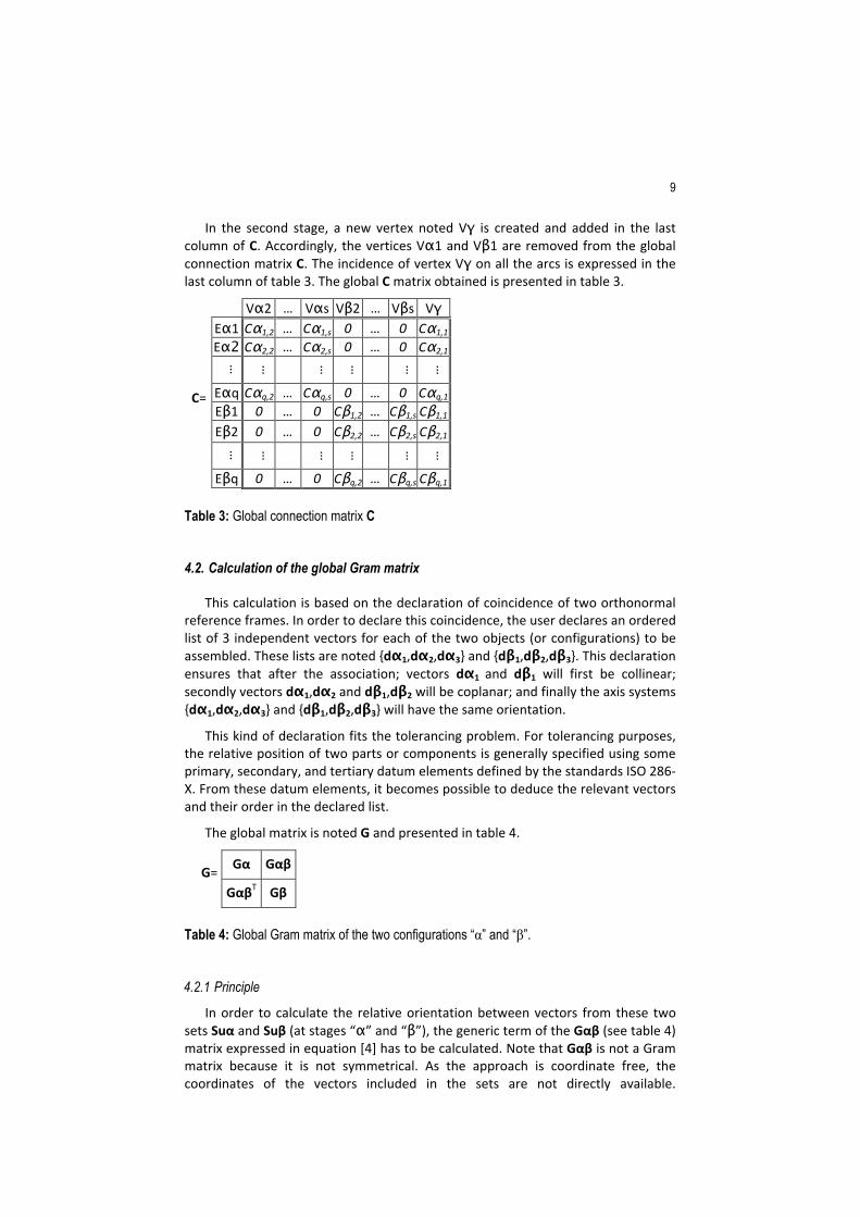
In the second stage, a new vertex noted Vγ is created and added in the last column of C. Accordingly, the vertices Vα1 and Vβ1 are removed from the global connection matrix C. The incidence of vertex Vγ on all the arcs is expressed in the last column of table 3. The global C matrix obtained is presented in table 3.
Vα2 … Vαs Vβ2 … Vβs Vγ Eα1 Cα1,2 … Cα1,s 0 … 0 Cα1,1 Eα2 Cα2,2 … Cα2,s 0 … 0 Cα2,1
…
… …
… …
…
Eαq Cαq,2 … Cαq,s 0 … 0 Cαq,1 Eβ1 0 … 0 Cβ1,2 … Cβ1,s Cβ1,1 Eβ2 0 … 0 Cβ2,2 … Cβ2,s Cβ2,1
…
… …
… …
…
C=
Eβq 0 … 0 Cβq,2 … Cβq,s Cβq,1
Table 3: Global connection matrix C
4.2. Calculation of the global Gram matrix
This calculation is based on the declaration of coincidence of two orthonormal reference frames. In order to declare this coincidence, the user declares an ordered list of 3 independent vectors for each of the two objects (or configurations) to be assembled. These lists are noted {dα1,dα2,dα3} and {dβ1,dβ2,dβ3}. This declaration ensures that after the association; vectors dα1 and dβ1 will first be collinear; secondly vectors dα1,dα2 and dβ1,dβ2 will be coplanar; and finally the axis systems {dα1,dα2,dα3} and {dβ1,dβ2,dβ3} will have the same orientation.
This kind of declaration fits the tolerancing problem. For tolerancing purposes, the relative position of two parts or components is generally specified using some primary, secondary, and tertiary datum elements defined by the standards ISO 286-‐X. From these datum elements, it becomes possible to deduce the relevant vectors and their order in the declared list.
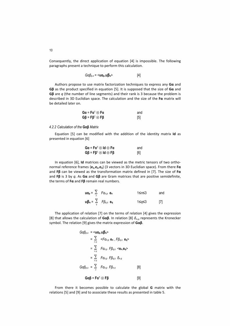
The global matrix is noted G and presented in table 4.
Gα Gαβ G=
GαβT Gβ
Table 4: Global Gram matrix of the two configurations “α” and “β”.
4.2.1 Principle
In order to calculate the relative orientation between vectors from these two sets Suα and Suβ (at stages “α” and “β”), the generic term of the Gαβ (see table 4) matrix expressed in equation [4] has to be calculated. Note that Gαβ is not a Gram matrix because it is not symmetrical. As the approach is coordinate free, the coordinates of the vectors included in the sets are not directly available.
10
Consequently, the direct application of equation [4] is impossible. The following paragraphs present a technique to perform this calculation.
4 Gαβp,s = <uαp,uβs> [4]
Authors propose to use matrix factorization techniques to express any Gα and Gβ as the product specified in equation [5]. It is supposed that the size of Gα and Gβ are q (the number of line segments) and their rank is 3 because the problem is described in 3D Euclidian space. The calculation and the size of the Fα matrix will be detailed later on.
5 Gα = FαT ⊗ Fα and Gβ = FβT ⊗ Fβ [5]
4.2.2 Calculation of the Gαβ Matrix
Equation [5] can be modified with the addition of the identity matrix Id as presented in equation [6]
6 Gα = FαT ⊗ Id ⊗ Fα and Gβ = FβT ⊗ Id ⊗ Fβ [6]
In equation [6], Id matrices can be viewed as the metric tensors of two ortho-‐normal reference frames {e1,e2,e3} (3 vectors in 3D Euclidian space). From there Fα and Fβ can be viewed as the transformation matrix defined in [7]. The size of Fα and Fβ is 3 by q. As Gα and Gβ are Gram matrices that are positive semidefinite, the terms of Fα and Fβ remain real numbers.
7 uαp =
€
n∑ Fαn,p en 1≤n≤3 and
uβs =
€
q∑ Fβq,s eq 1≤q≤3 [7]
The application of relation [7] on the terms of relation [4] gives the expression [8] that allows the calculation of Gαβ. In relation [8] δn,q represents the Kronecker symbol. The relation [9] gives the matrix expression of Gαβ.
8 Gαβp,s = <uαp,uβs>
=
€
n, q∑ <Fαn,p en , Fβq,s eq>
=
€
n, q∑ Fαn,p Fβq,s <en,eq>
=
€
n, q∑ Fαn,p Fβq,s δn,q
Gαβp,s =
€
n∑ Fαn,p Fβn,s [8]
9 Gαβ = FαT ⊗ Fβ [9]
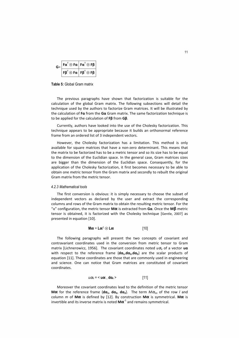
From there it becomes possible to calculate the global G matrix with the relations [5] and [9] and to associate these results as presented in table 5.
11
FαT ⊗ Fα FαT ⊗ Fβ G=
FβT ⊗ Fα FβT ⊗ Fβ
Table 5: Global Gram matrix
The previous paragraphs have shown that factorization is suitable for the calculation of the global Gram matrix. The following subsections will detail the technique used by the authors to factorize Gram matrices. It will be illustrated by the calculation of Fα from the Gα Gram matrix. The same factorization technique is to be applied for the calculation of Fβ from Gβ.
Currently, authors have looked into the use of the Cholesky factorization. This technique appears to be appropriate because it builds an orthonormal reference frame from an ordered list of 3 independent vectors.
However, the Cholesky factorization has a limitation. This method is only available for square matrices that have a non-‐zero determinant. This means that the matrix to be factorized has to be a metric tensor and so its size has to be equal to the dimension of the Euclidian space. In the general case, Gram matrices sizes are bigger than the dimension of the Euclidian space. Consequently, for the application of the Cholesky factorization, it first becomes necessary to be able to obtain one metric tensor from the Gram matrix and secondly to rebuilt the original Gram matrix from the metric tensor.
4.2.3 Mathematical tools
The first conversion is obvious: it is simply necessary to choose the subset of independent vectors as declared by the user and extract the corresponding columns and rows of the Gram matrix to obtain the resulting metric tensor. For the “α” configuration, the metric tensor Mα is extracted from Gα. Once the Mβ metric tensor is obtained, it is factorized with the Cholesky technique [Gentle, 2007] as presented in equation [10].
10 Mα = LαT ⊗ Lα [10]
The following paragraphs will present the two concepts of covariant and contravariant coordinates used in the conversion from metric tensor to Gram matrix [Lichnerowicz, 1956]. The covariant coordinates noted uαk of a vector uα with respect to the reference frame {dα1,dα2,dα3} are the scalar products of equation [11]. These coordinates are those that are commonly used in engineering and science. One can notice that Gram matrices are constituted of covariant coordinates.
11 uαk = < uα , dαk > [11]
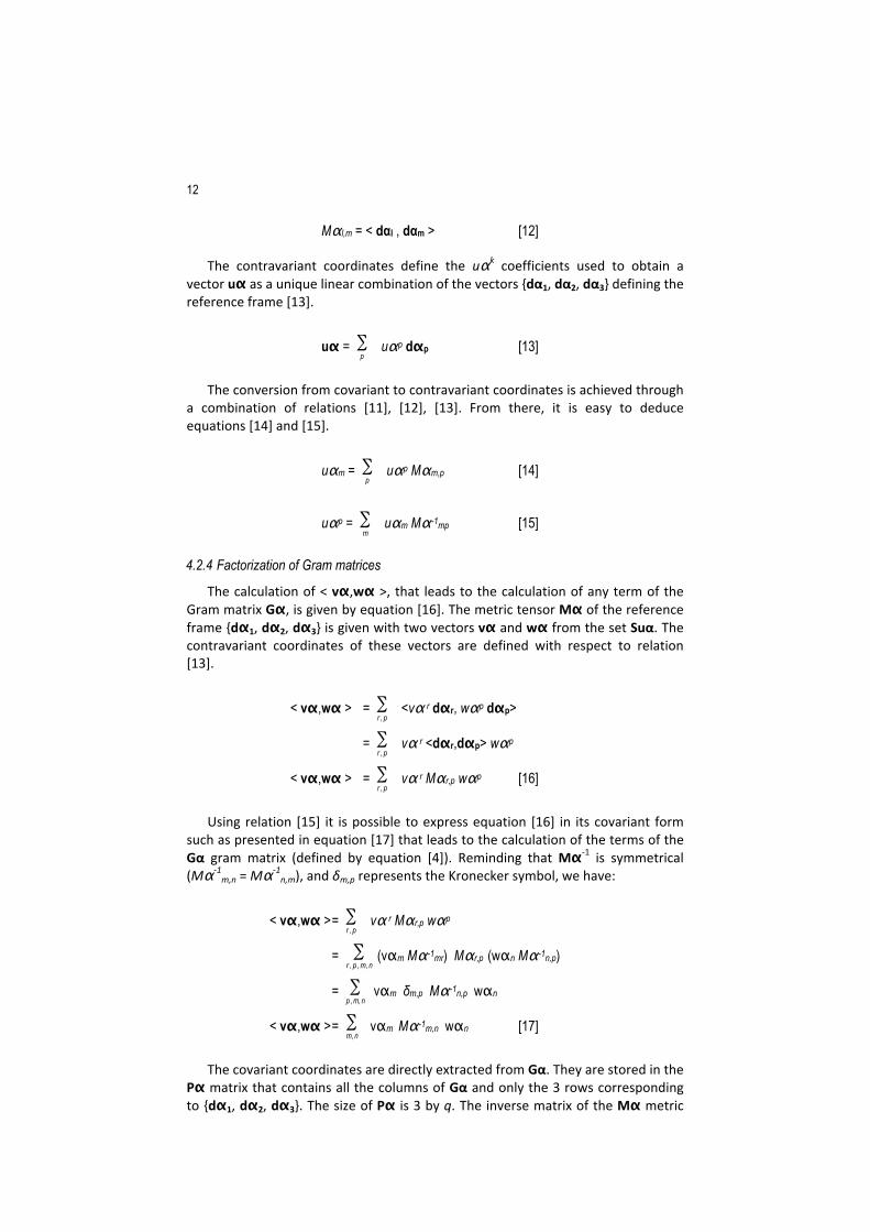
Moreover the covariant coordinates lead to the definition of the metric tensor Mα for the reference frame {dα1, dα2, dα3}. The term Mαlm of the row l and column m of Mα is defined by [12]. By construction Mα is symmetrical. Mα is invertible and its inverse matrix is noted Mα-‐1 and remains symmetrical.
12
12 Mαl,m = < dαl , dαm > [12]
The contravariant coordinates define the uαk coefficients used to obtain a vector uα as a unique linear combination of the vectors {dα1, dα2, dα3} defining the reference frame [13].
13 uα =
€
p∑ uαp dαp [13]
The conversion from covariant to contravariant coordinates is achieved through a combination of relations [11], [12], [13]. From there, it is easy to deduce equations [14] and [15].
14 uαm =
€
p∑ uαp Mαm,p [14]
15 uαp =
€
m∑ uαm Mα-1mp [15]
4.2.4 Factorization of Gram matrices
The calculation of < vα,wα >, that leads to the calculation of any term of the Gram matrix Gα, is given by equation [16]. The metric tensor Mα of the reference frame {dα1, dα2, dα3} is given with two vectors vα and wα from the set Suα. The contravariant coordinates of these vectors are defined with respect to relation [13].
16 < vα,wα > =
€
r , p∑ <vα r dαr, wαp dαp>
=
€
r , p∑ vα r <dαr,dαp> wαp
< vα,wα > =
€
r , p∑ vα r Mαr,p wαp [16]
Using relation [15] it is possible to express equation [16] in its covariant form such as presented in equation [17] that leads to the calculation of the terms of the Gα gram matrix (defined by equation [4]). Reminding that Mα-‐1 is symmetrical (Mα-‐1
m,n = Mα-‐1n,m), and δm,p represents the Kronecker symbol, we have:
17 < vα,wα > =
€
r , p∑ vα r Mαr,p wαp
=
€
r , p , m, n∑ (vαm Mα-1mr) Mαr,p (wαn Mα-1n,p)
=
€
p , m, n∑ vαm δm,p Mα-1n,p wαn
< vα,wα > =
€
m, n∑ vαm Mα-1m,n wαn [17]
The covariant coordinates are directly extracted from Gα. They are stored in the Pα matrix that contains all the columns of Gα and only the 3 rows corresponding to {dα1, dα2, dα3}. The size of Pα is 3 by q. The inverse matrix of the Mα metric
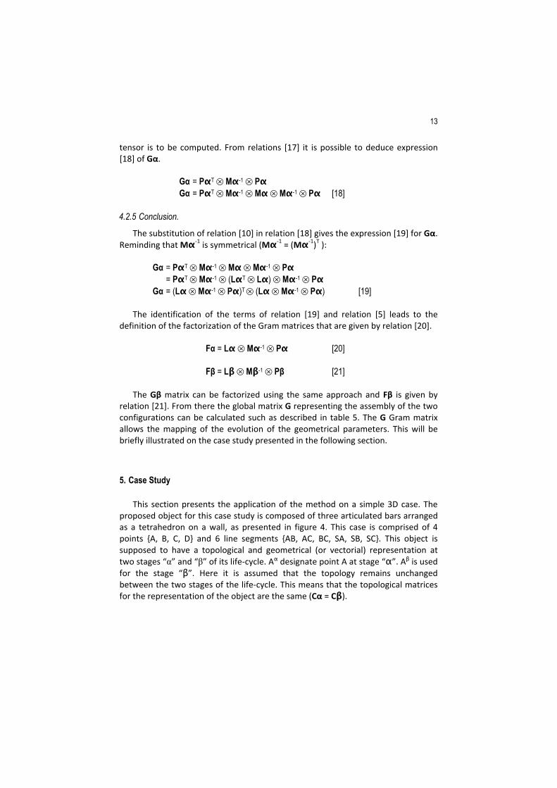
13 tensor is to be computed. From relations [17] it is possible to deduce expression [18] of Gα.
18 Gα = PαT ⊗ Mα-1 ⊗ Pα Gα = PαT ⊗ Mα-1 ⊗ Mα ⊗ Mα-1 ⊗ Pα [18]
4.2.5 Conclusion.
The substitution of relation [10] in relation [18] gives the expression [19] for Gα. Reminding that Mα-‐1 is symmetrical (Mα-‐1 = (Mα-‐1)T ):
19 Gα = PαT ⊗ Mα-1 ⊗ Mα ⊗ Mα-1 ⊗ Pα = PαT ⊗ Mα-1 ⊗ (LαT ⊗ Lα) ⊗ Mα-1 ⊗ Pα Gα = (Lα ⊗ Mα-1 ⊗ Pα)T ⊗ (Lα ⊗ Mα-1 ⊗ Pα) [19]
The identification of the terms of relation [19] and relation [5] leads to the definition of the factorization of the Gram matrices that are given by relation [20].
20 Fα = Lα ⊗ Mα-1 ⊗ Pα [20]
21 Fβ = Lβ ⊗ Mβ-1 ⊗ Pβ [21]
The Gβ matrix can be factorized using the same approach and Fβ is given by relation [21]. From there the global matrix G representing the assembly of the two configurations can be calculated such as described in table 5. The G Gram matrix allows the mapping of the evolution of the geometrical parameters. This will be briefly illustrated on the case study presented in the following section.
5. Case Study
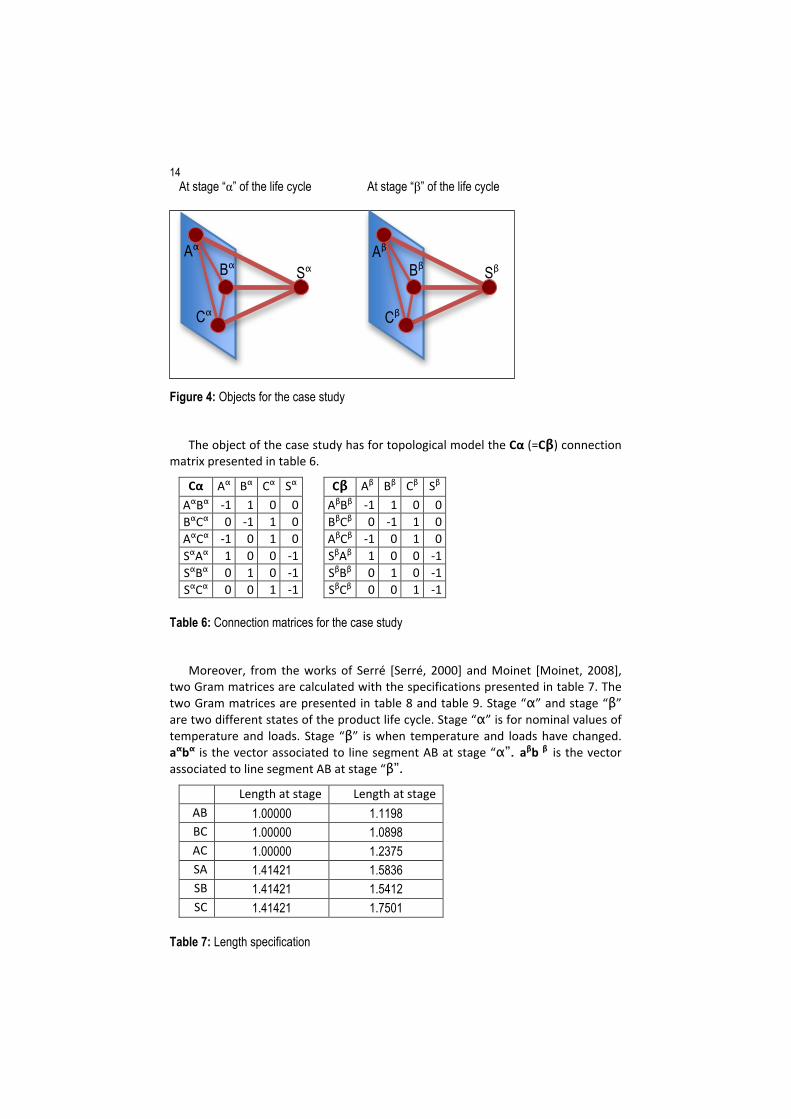
This section presents the application of the method on a simple 3D case. The proposed object for this case study is composed of three articulated bars arranged as a tetrahedron on a wall, as presented in figure 4. This case is comprised of 4 points {A, B, C, D} and 6 line segments {AB, AC, BC, SA, SB, SC}. This object is supposed to have a topological and geometrical (or vectorial) representation at two stages “α” and “β” of its life-‐cycle. Aα designate point A at stage “α”. Aβ is used for the stage “β”. Here it is assumed that the topology remains unchanged between the two stages of the life-‐cycle. This means that the topological matrices for the representation of the object are the same (Cα = Cβ).
14
Figure 4: Objects for the case study
The object of the case study has for topological model the Cα (=Cβ) connection matrix presented in table 6.
Cα Aα Bα Cα Sα Cβ Aβ Bβ Cβ Sβ
AαBα -‐1 1 0 0 AβBβ -‐1 1 0 0 BαCα 0 -‐1 1 0 BβCβ 0 -‐1 1 0 AαCα -‐1 0 1 0 AβCβ -‐1 0 1 0 SαAα 1 0 0 -‐1 SβAβ 1 0 0 -‐1 SαBα 0 1 0 -‐1 SβBβ 0 1 0 -‐1 SαCα 0 0 1 -‐1 SβCβ 0 0 1 -‐1
Table 6: Connection matrices for the case study
Moreover, from the works of Serré [Serré, 2000] and Moinet [Moinet, 2008], two Gram matrices are calculated with the specifications presented in table 7. The two Gram matrices are presented in table 8 and table 9. Stage “α” and stage “β” are two different states of the product life cycle. Stage “α” is for nominal values of temperature and loads. Stage “β” is when temperature and loads have changed. aαbα is the vector associated to line segment AB at stage “α”. aβb β is the vector associated to line segment AB at stage “β”.
Length at stage “α”
Length at stage “β” AB 1.00000 1.1198
BC 1.00000 1.0898 AC 1.00000 1.2375 SA 1.41421 1.5836 SB 1.41421 1.5412 SC 1.41421 1.7501
Table 7: Length specification
Bβ
Cβ
Sβ Bα
Cα
Sα
At stage “α” of the life cycle At stage “β” of the life cycle
Aα Aβ
15
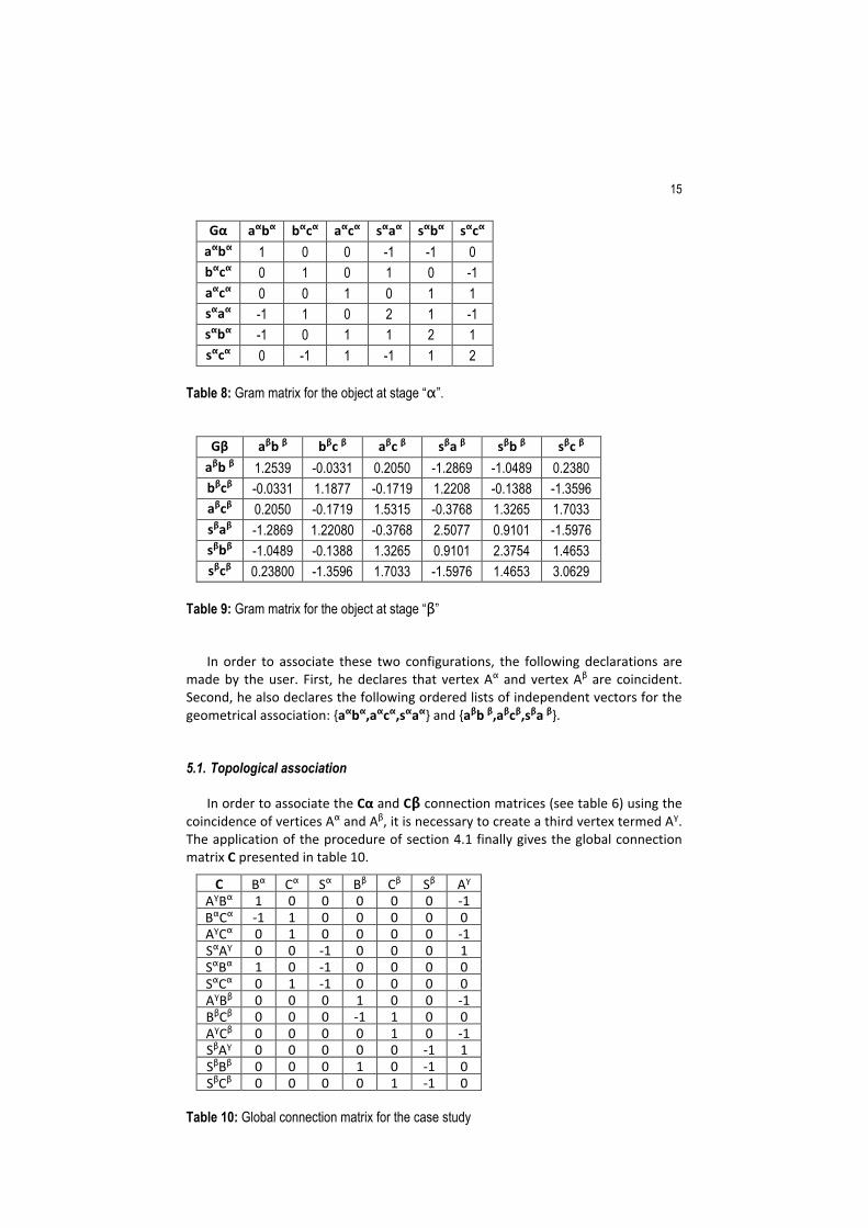
Gα aαbα bαcα aαcα sαaα sαbα sαcα aαbα 1 0 0 -1 -1 0 bαcα 0 1 0 1 0 -1 aαcα 0 0 1 0 1 1 sαaα -1 1 0 2 1 -1 sαbα -1 0 1 1 2 1 sαcα 0 -1 1 -1 1 2
Table 8: Gram matrix for the object at stage “α”.
Gβ aβb β bβc β aβc β sβa β sβb β sβc β
aβb β 1.2539 -0.0331 0.2050 -1.2869 -1.0489 0.2380 bβcβ -0.0331 1.1877 -0.1719 1.2208 -0.1388 -1.3596 aβcβ 0.2050 -0.1719 1.5315 -0.3768 1.3265 1.7033 sβaβ -1.2869 1.22080 -0.3768 2.5077 0.9101 -1.5976 sβbβ -1.0489 -0.1388 1.3265 0.9101 2.3754 1.4653 sβcβ 0.23800 -1.3596 1.7033 -1.5976 1.4653 3.0629
Table 9: Gram matrix for the object at stage “β”
In order to associate these two configurations, the following declarations are made by the user. First, he declares that vertex Aα and vertex Aβ are coincident. Second, he also declares the following ordered lists of independent vectors for the geometrical association: {aαbα,aαcα,sαaα} and {aβb β,aβcβ,sβa β}.
5.1. Topological association
In order to associate the Cα and Cβ connection matrices (see table 6) using the coincidence of vertices Aα and Aβ, it is necessary to create a third vertex termed Aγ. The application of the procedure of section 4.1 finally gives the global connection matrix C presented in table 10.
C Bα Cα Sα Bβ Cβ Sβ Aγ AγBα 1 0 0 0 0 0 -‐1 BαCα -‐1 1 0 0 0 0 0 AγCα 0 1 0 0 0 0 -‐1 SαAγ 0 0 -‐1 0 0 0 1 SαBα 1 0 -‐1 0 0 0 0 SαCα 0 1 -‐1 0 0 0 0 AγBβ 0 0 0 1 0 0 -‐1 BβCβ 0 0 0 -‐1 1 0 0 AγCβ 0 0 0 0 1 0 -‐1 SβAγ 0 0 0 0 0 -‐1 1 SβBβ 0 0 0 1 0 -‐1 0 SβCβ 0 0 0 0 1 -‐1 0
Table 10: Global connection matrix for the case study
16
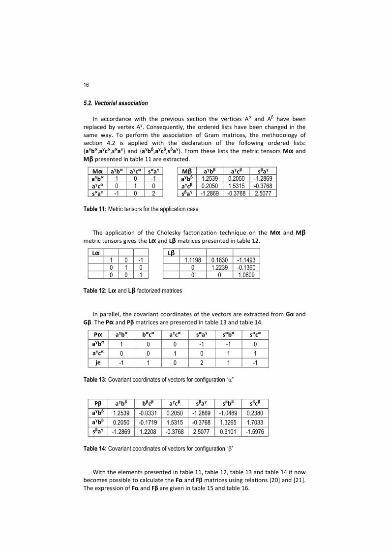
5.2. Vectorial association
In accordance with the previous section the vertices Aα and Aβ have been replaced by vertex Aγ. Consequently, the ordered lists have been changed in the same way. To perform the association of Gram matrices, the methodology of section 4.2 is applied with the declaration of the following ordered lists: {aγbα,aγcα,sαaγ} and {aγbβ,aγcβ,sβaγ}. From these lists the metric tensors Mα and Mβ presented in table 11 are extracted.
Mα aγbα aγcα sαaγ Mβ aγbβ aγcβ sβaγ aγbα 1 0 -1 aγbβ 1.2539 0.2050 -1.2869 aγcα 0 1 0 aγcβ 0.2050 1.5315 -0.3768 sαaγ -1 0 2 sβaγ -1.2869 -0.3768 2.5077
Table 11: Metric tensors for the application case
The application of the Cholesky factorization technique on the Mα and Mβ metric tensors gives the Lα and Lβ matrices presented in table 12.
Lα Lβ 1 0 -1 1.1198 0.1830 -1.1493 0 1 0 0 1.2239 -0.1360 0 0 1 0 0 1.0809
Table 12: Lα and Lβ factorized matrices
In parallel, the covariant coordinates of the vectors are extracted from Gα and Gβ. The Pα and Pβ matrices are presented in table 13 and table 14.
Pα aγbα bαcα aγcα sαaγ sαbα sαcα aγbα 1 0 0 -1 -1 0 aγcα 0 0 1 0 1 1 je -1 1 0 2 1 -1
Table 13: Covariant coordinates of vectors for configuration “α”
Pβ aγbβ bβcβ aγcβ sβaγ sβbβ sβcβ aγbβ 1.2539 -0.0331 0.2050 -1.2869 -1.0489 0.2380 aγbβ 0.2050 -0.1719 1.5315 -0.3768 1.3265 1.7033 sβaγ -1.2869 1.2208 -0.3768 2.5077 0.9101 -1.5976
Table 14: Covariant coordinates of vectors for configuration “β”
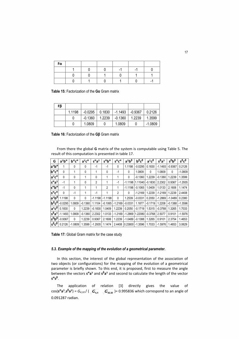
With the elements presented in table 11, table 12, table 13 and table 14 it now becomes possible to calculate the Fα and Fβ matrices using relations [20] and [21]. The expression of Fα and Fβ are given in table 15 and table 16.
17
Fα 1 0 0 -1 -1 0 0 0 1 0 1 1 0 1 0 1 0 -1
Table 15: Factorization of the Gα Gram matrix
Fβ
1.1198 -0.0295 0.1830 -1.1493 -0.9367 0.2126
0 -0.1360 1.2239 -0.1360 1.2239 1.3599
0 1.0809 0 1.0809 0 -1.0809
Table 16: Factorization of the Gβ Gram matrix
From there the global G matrix of the system is computable using Table 5. The result of this computation is presented in table 17.
G aγbα bαcα aγcα sαaγ sαbα sαcα aγbβ bβcβ aγcβ sβaγ sβbβ sβcβ aγbα 1 0 0 -1 -1 0 1.1198 -0.0295 0.1830 -1.1493 -0.9367 0.2126
bαcα 0 1 0 1 0 -1 0 1.0809 0 1.0809 0 -1.0809
aγcα 0 0 1 0 1 1 0 -0.1360 1.2239 -0.1360 1.2239 1.3599
sαaγ -1 1 0 2 1 -1 -1.1198 1.11040 -0.1830 2.2302 0.9367 -1.2935
sαbα -1 0 1 1 2 1 -1.1198 -0.1065 1.0409 1.0133 2.1606 1.1474
sαcα 0 -1 1 -1 1 2 0 -1.2169 1.2239 -1.2169 1.2239 2.4408
aγbβ 1.1198 0 0 -1.1198 -1.1198 0 1.2539 -0.0331 0.2050 -1.2869 -1.0489 0.2380
bβcβ -0.0295 1.0809 -0.1360 1.1104 -0.1065 -1.2169 -0.0331 1.1877 -0.1719 1.2208 -0.1388 -1.3596
aγcβ 0.1830 0 1.2239 -0.1830 1.0409 1.2239 0.2050 -0.1719 1.5315 -0.3768 1.3265 1.7033
sβaγ -1.1493 1.0809 -0.1360 2.2302 1.0133 -1.2169 -1.2869 1.22080 -0.3768 2.5077 0.9101 -1.5976
sβbβ -0.9367 0 1.2239 0.9367 2.1606 1.2239 -1.0489 -0.1388 1.3265 0.9101 2.3754 1.4653
sβcβ 0.2126 -1.0809 1.3599 -1.2935 1.1474 2.4408 0.23800 -1.3596 1.7033 -1.5976 1.4653 3.0629
Table 17: Global Gram matrix for the case study
5.3. Example of the mapping of the evolution of a geometrical parameter.
In this section, the interest of the global representation of the association of two objects (or configurations) for the mapping of the evolution of a geometrical parameter is briefly shown. To this end, it is proposed, first to measure the angle between the vectors sαaγ and sβaγ and second to calculate the length of the vector sαsβ.
The application of relation [3] directly gives the value of cos(sαaγ,sβaγ) = G4,10 / ( )= 0.995836 which correspond to an angle of
0.091287 radian.
18
From matrix C (see table 10),a possible path to go from vertex Sα to vertex Sβ is deduced as going through vertex Aγ. Consequently the scalar product <sαsβ,sαsβ> is expressed by relation [22].
22 <sαsβ,sαsβ> = <sαaγ,sαaγ> + 2 <sαaγ,aγsβ> + <aγsβ,aγsβ> <sαsβ,sαsβ> = <sαaγ, sαaγ> - 2 < sαaγ,sβaγ> + <sβaγ,sβaγ> <sαsβ,sαsβ> = G4,4 - 2 G4,10 + G10,10 [22]
The combination of relations [2] and [22] allows the calculation of ||sαsβ|| from the elements available in the global Gram matrix G presented in table 17. After calculation, the result obtained is ||sαsβ|| = 0.217565 length unit.
6. Conclusion and perspectives
This paper has first presented a generic model for representing objects using points and line segments exclusively. That description proved to be suitable for the representation of the skeleton of a mechanical product at the early stages of the design process. Secondly a means for representing objects, thanks to two matrices, was introduced. A connection matrix was used to indicate how points and line segments were connected and a Gram matrix is used to provide the user with lengths and orientation information about the line segments. In the third part, the paper showed how to perform an assembly with two objects represented with these two matrices. Finally, the interest of this model for the mapping of the evolution of a geometrical parameter has been exhibited on a case study.
In terms of future work, the authors propose first to consider the addition of surface elements such as triangles to enhance the possibilities for modelling complex objects. Secondly, it is also envisaged to implement additional constraints, such as topological coincidence between two lines segments, for the declaration of the assembly of the two objects.
7. Bibliography
Anselmetti B., Generation of functional tolerancing based on positioning features. Computer-‐Aided Design, 38(8):902–919, Aug 2006.
Gentle J. E., Matrix Algebra: Theory, Computations, and Applications in Statistics. Springer, 2007.
Ghie W., Modèle unifié jacobien-‐torseur pour le tolérancement assisté par ordinateur, 2004.
Lichnerowicz A., Algèbre et analyse linéaires. Masson Paris, second edition, 1956.
Louhichi B., Intégration CAO/Calcul par reconstruction du modèle CAO à partir des résultats éléments finis. PhD thesis, 2008.
M'henni F., Effet des tolérances géométriques qualitatives et quantitatives sur le comportement d’un mécanisme : critères d’évaluation. PhD thesis, Tunisie, 2010.
19 Moinet M., Serré P., Rivière A., Clément A., A new approach to transform a constrained
geometric object. In Proceedings of the 20th CIRP Design Conference, Nantes, France, April 19–21, 2010. Best paper award.
Moinet M., Descriptions non cartésiennes et résolution de problèmes géométriques sous contraintes. PhD thesis, École Centrale Paris, December 2008.
Pierre L., Teissandier D., Nadeau J.-‐P., Integration of multiple physical behaviours into a geometric tolerancing approach. 2009.
Serré P., Ortuzar A., Rivière A., Non-‐cartesian modelling for analysis of the consistency of a geometric specification for conceptual design. International Journal of Computational Geometry & Applications, 16(5/6):549–565, 2006.
Serré P., Cohérence de la spécification d'un objet de l'espace euclidien à n dimensions. PhD thesis, École Centrale Paris, April 2000.
Recommended