C.A. Torres March, 2008
Geometric Characterisation of Rock Mass Discontinuities Using Terrestrial Laser Scanner
and Ground Penetrating Radar
Disco
Thesis ObservatioGeo-inform
The Dr. Dr.iDr. Dr. Drs
INTERNATI
Geomeontinuit
submitted toon in partial mation Scien
esis Assessm
F.D. van der. E.C. Slob,H.R.G.K. HaM. van der M. T.M. Loran
IONAL INSTI
etric Chies UsinGroun
o the Internafulfilment of
nce and Ear
ment Board
r Meer, Cha, External Exack, First SuMeijde, Secon, Course Di
TUTE FOR GENSC
aractering Terred Penet
by
C.A. T
ational Instituf the requiremrth Observat
airman xaminer upervisor ond Supervirector AES
GEO-INFORMCHEDE, THE
isation oestrial Ltrating R
y
Torres
ute for Geo-iments for thion, Special
sor
MATION SCIENETHERLAN
of RockLaser ScRadar
nformation Se degree of isation: (Ear
ENCE AND ENDS
k Mass canner
Science andMaster of S
rth Applied S
EARTH OBSE
and
d Earth cience in
Sciences)
ERVATION

Disclaimer
This document describes work undertaken as part of a programme of study at the International Institute for Geo-information Science and Earth Observation. All views and
opinions expressed therein remain the sole responsibility of the author, and do not necessarily represent those of the institute.

i
Abstract
A main objective of the geometric characterization of rock mass discontinuities is to establish a three dimensional model that permits to define the fabric of this discontinuous medium. Because of the existing limitations in field surveys and data processing methods it is necessary to extract as much information as possible in an integrated and objective way in order to create a more consistent model of the rock mass fabric while decreasing the degree of uncertainty. The use of Terrestrial Laser Scanner (TLS) has shown to be an attractive and consistent alternative to digitally reconstruct the exposed surface of a rock mass outcrop and acquire geometric information through a semi-automated extraction of the geometric properties (orientation and spacing). On the other hand, Ground Penetrating Radar (GPR) based methods have allowed to detect and map internal discontinuities and derive a interpretation of a rock mass internal discontinuities network. The objective of the research is to determine whether the geometric information derived from TLS and GPR can be integrated and used in a geometric characterization of a rock mass and how this can improve traditional survey methods. Traditional, TLS and GPR surveys were performed over a rock slope at a porphyry stone quarry (Trento, North Italy). Traditional, TLS and GPR derived data were processed separately in order to obtain geometric information; this information was integrated while following geometric characterization. The individual results and the integrated analysis of the geometrical information derived from Terrestrial Laser Scanner and Ground Penetrating Radar showed a reasonable degree of correlation with the results of the traditional approach and demonstrated to be an attractive way of complement such information in order to reduce the degree of uncertainty about the geometrical characteristics of the discontinuity network of a rock mass.

ii
Acknowledgements
I would like to express my gratitude to my supervisors Dr. Robert Hack and Dr. Mark van der Meijde. I also grateful to all the ITC and Nuffic Organization. I wish to acknowledge to Dr. Antonio Galgaro, Dr. Giordano Teza and Geol. Annapaola Gradizzi from the Department of Geology, Palaeontology and Geophysics of the University of Padova (Padova, Italy) who provided the equipment and offer technical expertise along the field campaign. Andrei Torres Enschede, 2008
iii
Table of contents
1. Introduction ....................................................................................................................... 9
1.1. Scope ........................................................................................................................ 9 1.2. Problem definition .................................................................................................... 10 1.3. Research question .................................................................................................. 10 1.4. Research objective .................................................................................................. 11 1.5. Specific objectives ................................................................................................... 11 1.6. General Methodology .............................................................................................. 11
2. Modelling the geometry of a discontinuity network in a rock mass ................................. 12 2.1. Discontinuity definition ............................................................................................. 12 2.2. Geometric properties of discontinuities ................................................................... 13 2.3. Traditional methods to collecting discontinuity data ................................................ 14
2.3.1. Surface methods .............................................................................................. 14 2.3.2. Subsurface methods - borehole explorations ................................................... 15
2.4. Terrestrial Laser Scanner as a recent technique to derive geometric information .. 15 2.4.1. TLS fundamentals ............................................................................................ 15 2.4.2. Data processing ............................................................................................... 15
2.5. Ground Penetrating Radar based methodologies for detect internal discontinuities 18 2.5.1. Ground Penetrating Radar fundamentals ........................................................ 18 2.5.2. Ground Penetrating Radar as a technique to detect internal discontinuities.... 19 2.5.3. GPR data processing methodology ................................................................. 20
2.6. Discontinuity network modelling .............................................................................. 20 2.6.1. Discontinuity sets and homogeneous regions .................................................. 21 2.6.2. Discontinuity orientation ................................................................................... 22 2.6.3. Discontinuity spacing ....................................................................................... 24 2.6.4. Trace length and persistence ........................................................................... 25
2.7. Discontinuity network modelling and validation ....................................................... 26 3. Methodology ................................................................................................................... 27
3.1. Study site ................................................................................................................. 28 3.2. Weather, seepage groundwater conditions ............................................................. 29 3.3. Geometric characterization, traditional approach .................................................... 30
3.3.1. Slope Stability Probability Classification (SSPC) ............................................. 30 3.3.2. Scanline Survey ............................................................................................... 31 3.3.3. Validation and integration of the derived information ....................................... 33
4. Geometric characterization, TLS based methods .......................................................... 35 4.1. Data acquisition ....................................................................................................... 35 4.2. Dataset reorientation ............................................................................................... 36 4.3. Data analysis to derive orientation information ....................................................... 36
4.3.1. Surface reconstruction with 2D gridding and Delaunay triangulation ............... 36 4.3.2. Direct segmentation with 3D Hough transformation and least squares ........... 41
iv
4.4. Validation of Terrestrial Laser Scanner Mehtods against Traditional Approaches .. 47 4.5. Deriving spacing information ................................................................................... 52
5. Detecting and mapping internal discontinuity network, Ground Penetrating Radar based method ................................................................................................................................... 53
5.1. Methodology ............................................................................................................ 53 5.2. Establishing GPR viability and GPR survey requirements ...................................... 54
5.2.1. GPR survey objective ....................................................................................... 54 5.2.2. Rock mass characteristics ................................................................................ 54 5.2.3. GPR performance for detecting discontinuities ................................................ 55 5.2.4. Survey requirements ........................................................................................ 56
5.3. Data adqusition ........................................................................................................ 57 5.4. GPR data processing .............................................................................................. 58
5.4.1. GPR raw data characteristics ........................................................................... 58 5.4.2. GPR data processing ....................................................................................... 59
5.5. Results interpretation ............................................................................................... 60 5.6. Results validation .................................................................................................... 64
6. Integration of the geometric information derived from TLS and GPR and validation against the traditional approach ............................................................................................. 65
6.1. TLS and GPR derived information integration ......................................................... 65 6.2. Validation against the traditional approach .............................................................. 65
6.2.1. Discontinuity set J1 .......................................................................................... 66 6.2.2. Discontinuity set J2 .......................................................................................... 66 6.2.3. Discontinuity set J3 .......................................................................................... 67 6.2.4. Discontinuity set J4 .......................................................................................... 67 6.2.5. Discontinuity set J5 .......................................................................................... 67 6.2.6. Discontinuity set J6 .......................................................................................... 67
6.3. General observations .............................................................................................. 68 6.3.1. Number of discontinuity sets ............................................................................ 68 6.3.2. Discontinuity sets orientation ............................................................................ 68 6.3.3. Normal discontinuity set spacing ...................................................................... 68 6.3.4. Discontinuity sets persistence .......................................................................... 69
7. Conclusions .................................................................................................................... 69 7.1. Terrestrial Laser Scanner method ........................................................................... 69 7.2. Ground penetrating radar ........................................................................................ 70
References ............................................................................................................................. 71
v
List of figures
Figure 1. General Methodology flowchart Figure 2. Geometric properties in a discontinuous rock mass (after (Hudson, 1989)) Figure 3. a) Rock mass scanned surface, b) Polygonal surface reconstruction Figure 4. a) Rock mass scanned surface, b) Segmented TLS point cloud data Figure 5. a) Rock mass scanned surface, b) Surface reconstruction and c) Equal area hemispherical projection of all facet poles grouped using fuzzy k-means clustering (see section 2.6.2), (Slob and van Knapen, 2006) Figure 6. Illustration of the processing applied to GPR data a) Raw data, b) Processed data using i) a DC removal ,ii) a zero-phase band-pass filter and iii) an AGC time equalization. (c) Static corrections for topography and time to depth conversion were applied, d) Interpretation of the discontinuity network (Deparis et al., 2007) Figure 7. Stereographic projection of the pole of a plane: (a) Reference sphere, b) Hemispherical projection, c) Stereonet representation (after (Brady and Brown, 2004)). Figure 8. Some examples of orientation models Figure 9. General methodology flowchart Figure 10. Study site at Albiano (Province of Trento, North Italy) a) Porphyry quarry (Permian Rhyolite), b) Location, c) geological map Figure 11. Rock mass exposure at Albiano quarry (Permian Rhyolite), height ≈ 20m. Figure 12. Scanline survey Figure 13. Low hemisphere, equal angle stereo-plot and density of orientation data (poles) obtained from SSPC (in red) and scanline survey (orientation data in black and kernel density in grey scale) Figure 14. a) Laser scanner campaign. b) Cropped TLS dataset: 1.993.314 points (displayed by intensity value) Figure 15. TLS data process for deriving geometric information through surface reconstruction using 2D gridding and Delaunay triangulation Figure 16. Original point cloud data and surface reconstruction through 2D gridding and Delaunay triangulation (Software: Split-FX® Ver.1.0) Figure 17.Surface reconstruction through 2D gridding and Delaunay triangulation and result of planes patterns recognition. Isolated plane patterns are displayed in blue, and excluded areas in red. (Software: Split-FX® Ver.1.0). Figure 18. Lower hemisphere, equal area stereo-plot and density of orientation data (poles). a) Traditional methods: SSPC (red squares), Scanline (black signs). b) Surface reconstruction method (blue points).(Software: Dips Ver. 5.106 ®, Split-FX® Ver.1.0). Figure 19. TLS data process for deriving geometric information direct segmentation and least squares estimation Figure 20. Original point cloud data and direct segmentation results through Figure 21. Low hemisphere, equal area stereo-plot and density of orientation data (poles). a) Traditional methods: SSPC (red squares), Scanline (black signs). b) Direct segmentation (black signs). (Software: Dips Ver. 5.106 ®)

vi
Figure 22. Low hemisphere, equal area stereo-plot and density of orientation data (poles). a) Traditional methods: SSPC (red squares), Scanline (black signs), b) Surface reconstruction and c) Direct segmentation (black signs). (Software: Dips Ver. 5.106 ®, Split FX ® Ver.1.0) Figure 23. GPR methodology for detect and map internal discontinuity network Figure 24. GPR survey setting Figure 25. GPR raw data (profile H3). Data is dominated by direct air wave (A), ground wave (B), system ringing (C), multiples (D) and diffraction hyperbolas (E). Figure 26. GPR raw data processing scheme Figure 27. Progressive results of applying processing scheme to a typical horizontal section (profile H3). a) Raw data, b) Geometry specification, static correction, and background removal, c) amplitude compensation, d) band-pass filtering, e) Running average and d) Time to depth conversion and migration. Blues/greens and reds/violets define negative and positive pulses and colour intensity is a function of amplitude.
vii
List of tables
Table 1. SSPC rock mass geometric description ( > denotes greater than the exposure size, see SSPC filed form details in appendix 1) Table 2. Descriptive statistics of the scanline surveys results (* Fisher k constant is not valid if the sample size N is smaller than 10) Table 3. Summary of geometric parameters derived from each method for each set Table 4. Parameter values used for surface reconstruction through 2D gridding and Delaunay triangulation (Software: Split-FX® Ver.1.0) Table 5. Parameter values used for surface reconstruction through 2D gridding and Delaunay triangulation Table 6. Summary of the orientation results: Traditional methods (SSPC and Scanline) versus surface reconstruction method. (* Fisher k constant is not valid if the sample size N is smaller than 10) Table 7. Kd-tree structure parameters (* Refers to the average number of points that each kd-tree cell contain) Table 8. Parameter values used for direct segmentation Table 9. Summary of the orientation results: Traditional methods (SSPC and Scanline) versus direct segmentation method. (* Fisher k constant is not valid if the sample size N is smaller than 10) Table 10. Summary orientation statistics. a) Traditional methods: SSPC, Scanline, b) Surface reconstruction and c) Direct segmentation Table 11. Summary of normal set spacing results, comparison between traditional and TLS (direct segmentation) method Table 12. Summary of the geometrical and condition characteristics of the Table 13. Properties of the acquired GPR profiles Table 14. Comparison between geometrical information derived from the interpretation of GPR profiles and SSPC characterization (the symbol > denotes that the persistence is lager than the characterized exposure or larger the GPR profile length) Table 15. Integration of geometric information derived from the remote sensing approach (the symbol > denotes that the persistence is lager than the characterized exposure or larger the GPR profile length). Table 16. Integration of geometric information derived from the remote sensing approach

9
1. Introduction
1.1. Scope
When dealing with discontinuous rock masses, the properties of the discontinuities in the rock becomes of prime importance, since they will determine, to a large extent, the mechanical behaviour of the rock mass (Bieniawski, 1989). These properties are classified into geometric and non-geometric. The non-geometric properties are related to mechanical behaviour of the infill material and the shear strength of the intact rock adjacent to the discontinuity while the geometric properties define the fabric of the discontinuous rock mass (Hack, 1998). The main objective of the geometric characterization of the discontinuities within a rock mass is to establish a model that permits to define the fabric of this discontinuous medium. Discontinuities are just partially accessible at their intersection with outcrops, boreholes and drifts from which analysis methods make assumptions about such discontinuity network. Variation in the performed field measurements and hence the model that is derived are constrained by the sampling technique is used, the degree of exposure the rock mass outcrop has and the number of observations that can be done (Priest and Hudson, 1981). Traditional techniques for geometric characterization of rock masses include scan line survey, cell mapping, and rapid face mapping to systematically direct the mapping of a rock face (Hack, 1998). These surface interpretation methods can be complemented by borehole surveys in order to achieve a better knowledge of the discontinuity network (Wines and Lilly, 2002). However these traditional methods are time consuming and often present some degree of error. New techniques for geometric characterization of discontinuities based on the interpretation of the visible surface of a rock mass outcrop include image analysis, digital photogrammetry and total station (Kemeny, 2003; Lemy and Hadjigeorgiou, 2003; Roncella and Forlani, 2005; Zhang et al., 2004). Among these new methods, Terrestrial Laser Scanner is a remote sensing technique which has shown a great potential to obtain a large quantity of accurate geometric data (Slob et al., 2004). A remarkable aspect is the possibility of reconstructing rock mass face and extracting geometrical information of such surface by analytical methods (Rotonda et al., 2007; Slob et al., 2004; Slob and van Knapen, 2006). On the other hand, Ground Penetrating Radar has been used to detect and map internal discontinuities in rock masses as an alternative to borehole exploration. After processing and interpreting the Ground Penetrating Radar data, a representation of the geometry of the internal discontinuities can be obtained. Comparison between discontinuities observed on surface and those mapped using Ground Penetrating Radar have shown reasonable correlation (Deparis and Garambois, 2006; Grandjean and Gourry, 1996; Porsani et al., 2006).

10
1.2. Problem definition
In order to perform a geometric characterization, traditional survey techniques have shown large disadvantages since they are time consuming, involve human bias, and present safety, access and economic constraints (Slob et al., 2004), however for most engineering problems the use of these techniques with a proper engineering judgement are considered to be enough and useful (Hack, 1998). Although comparison between Terrestrial Laser Scanner based and traditional methods have shown coherent results, difficulties have been reported associated with some unfavourable geometric configurations (i.e. angle of incidence of the laser beam and the identification of horizontal surfaces) (Roncella and Forlani, 2005; Rotonda et al., 2007). Hence, there is still a need for engineering criteria to provide manual intervention, spot checks and results interpretation (Coggan et al., 2007). On the other hand, Ground Penetrating Radar based methods to detect and map internal discontinuities have shown a good degree of correlation with surface observations when characterizing rock masses at quarry scale ((Grandjean and Gourry, 1996), but they are limited to the interpretation of 2D profiles in order to obtain a representation of the internal discontinuities and they require to be validated by gathering additional information (i.e. the results of the interpretation of GPR profiles must be validated with structural maps of the rock mass). Because of the existing limitations in field surveys and data processing methods it is necessary to extract as much information as possible in an integrated and objective way in order to create a more consistent model of the rock mass fabric while decreasing its degree of uncertainty.
1.3. Research question
The assumption behind the Terrestrial Laser Scanner technique is that the geometry of the discontinuities in the visible rock mass surface has a relation with the geometry of the discontinuities within the rock mass. As it has been discussed before, the geometric information is derived through an analytic process and comparisons between these results and those derived from the traditional approach have shown coherent results, but difficulties have been reported associated with some unfavourable geometric configurations. On the other hand, Ground Penetrating Radar technique has allowed detecting and mapping internal discontinuities based on the interpretation of the heterogeneities that can appear in two-dimensional profiles. However, while interpreting internal discontinuities, it is often necessary to use additional information to correlate such features and validated the final results. The research question that comes out when considering these facts is: Is it possible to analyse in an integrated way the geometric information resulting from Terrestrial Laser Scanner and Ground Penetrating Radar surveys in order to complement such information and to obtain a more consistent model of the fabric of a discontinuous rock mass?
11
1.4. Research objective
The research objective of the research is to determine whether the geometric information derived from Terrestrial Laser Scanner and Ground Penetrating Radar can be integrated and used in a geometric characterization of a rock mass, how this can improve traditional survey methods and how satisfactory is the output with comparing with a traditional engineering method.
1.5. Specific objectives
To derive geometric information from a Terrestrial Laser Scanner survey
To derive geometric information from a Ground Penetrating Radar survey
To analyze in an integrated way Terrestrial Laser Scanner and Ground Penetrating Radar geometric derived parameters in order to perform a geometric characterization of a rock slope.
To determine the consistency of the results of the proposed methodology when comparing with traditional ones such as SSPC (Hack, 1998) and scanline.
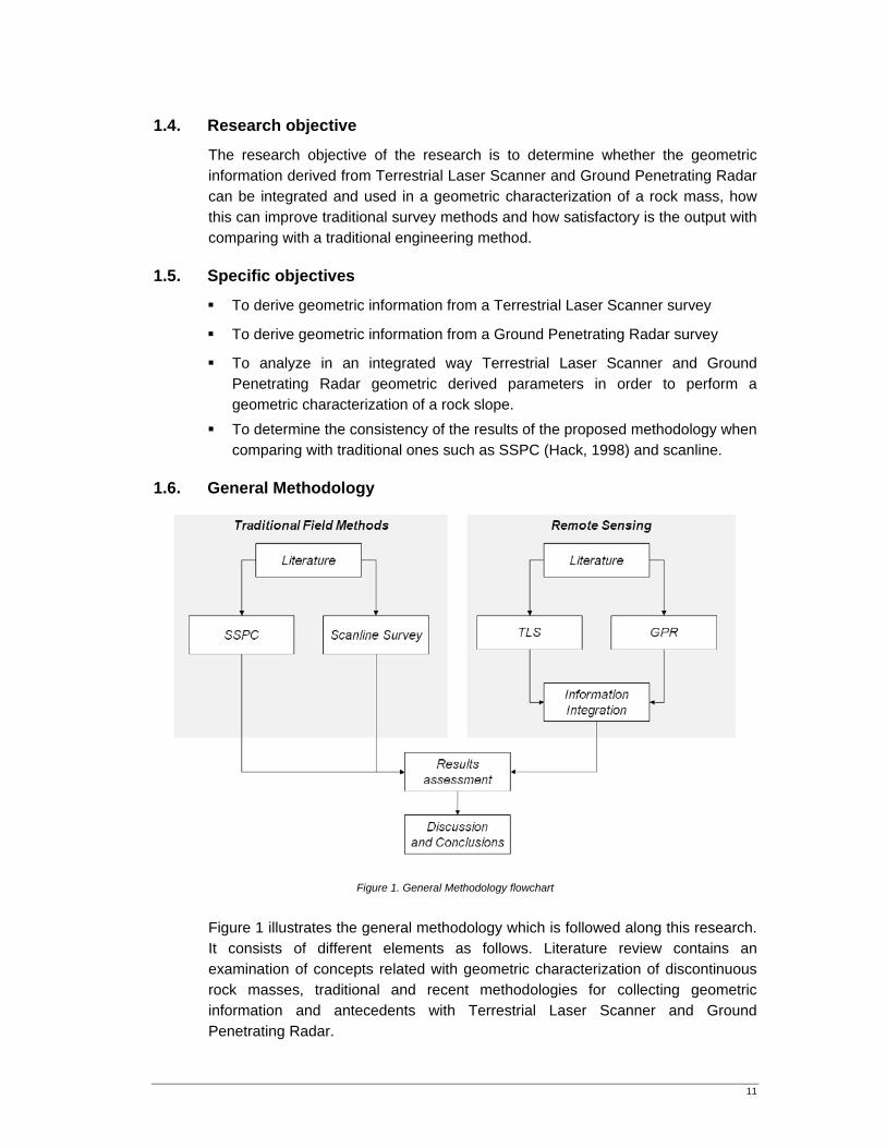
1.6. General Methodology
Figure 1. General Methodology flowchart Figure 1 illustrates the general methodology which is followed along this research. It consists of different elements as follows. Literature review contains an examination of concepts related with geometric characterization of discontinuous rock masses, traditional and recent methodologies for collecting geometric information and antecedents with Terrestrial Laser Scanner and Ground Penetrating Radar.
12
The dataset that is used through the research was acquired at rock slope in a porphyry stone quarry located at Albiano (South Italy). Traditional approaches (SSPC and scan-line) to characterize the rock mass exposure and remote sensing surveys (Ground Penetrating Radar and Terrestrial Laser Scanner) were performed all together in single field campaign. Remote sensing equipment was provided by the Department of Geology, Palaeontology and Geophysics of the University of Padova (Padova, Italy). In order to derive geometric parameters that are required in a geometric modelling schema, the data process is performed attending the methodologies and results of previous experiences as is established along the literature review. Terrestrial Laser Scanner and Ground Penetrating Radar derived information is finally integrated while following a geometric modelling schema, through the process traditional engineering criteria and statistical tools are used to determine whether the integrated analysis of this complemented information can improve the knowledge about the geometric characteristics of the rock mass and if this is consistent with traditional approach. Discussion and conclusions provides a summary of the research in terms of advantages, disadvantages, learned lessons, conclusions and recommendations for further research.
2. Modelling the geometry of a discontinuity network in a rock mass
2.1. Discontinuity definition
A discontinuity is a plane or surface that marks a change in physical or chemical characteristics in rock material (Hack, 1998). Discontinuities can be classified into mechanicals or integrals. A mechanical discontinuity denote a plane of physical weakness, this means that the tensile strength perpendicular to this surface or the shear strength along it are lower than those of the surrounding material (ISRM, 1981). Contrarily, an integral discontinuity is as strong as the surrounding material. Integral discontinuities can become mechanical due to weathering or chemical reactions that develop a change in mechanical properties (Hack, 1998). According to the geological process by which are discontinuities formed they can be classified as follows: Bedding planes: Typical of sedimentary rocks as a result of different
sedimentation cycles.
Joints: Produced by changes in stress condition due to geological processes. By definition, no movement has taken place in geological time along a joint.
Foliation: Formed by the tendency that some minerals have to grow in a specific orientation under the influence of stress and temperature. This occurs in metamorphic and igneous rocks.
13
Shears: Rocks deformed by folding often contain shears due to minor fault generation. These kinds of discontinuities are more spaced than joints (from few millimetres to as much as a meter) and are filled with soft or friable soil or rock.
Manmade discontinuities: Caused by blasting or mechanical excavation. They occur in a random manner due to breakage of intact rock blocks and generally are not persistent.
Faults: Present relative movement on either side of the fault and often all other discontinuities through. Faults occur mostly as an individual phenomenon.
Discontinuities show development patterns that are the result from the geological (and sometimes man-induced) processes through which they were formed. They can exist as single feature or as discontinuity sets. In theory, orientations and spacing of the planes discontinuities gather around a certain number of discontinuity sets with a distinctive orientation, spacing value and mechanical behaviour as result of a common geological origin (Goodman, 1989; Hack 1998).
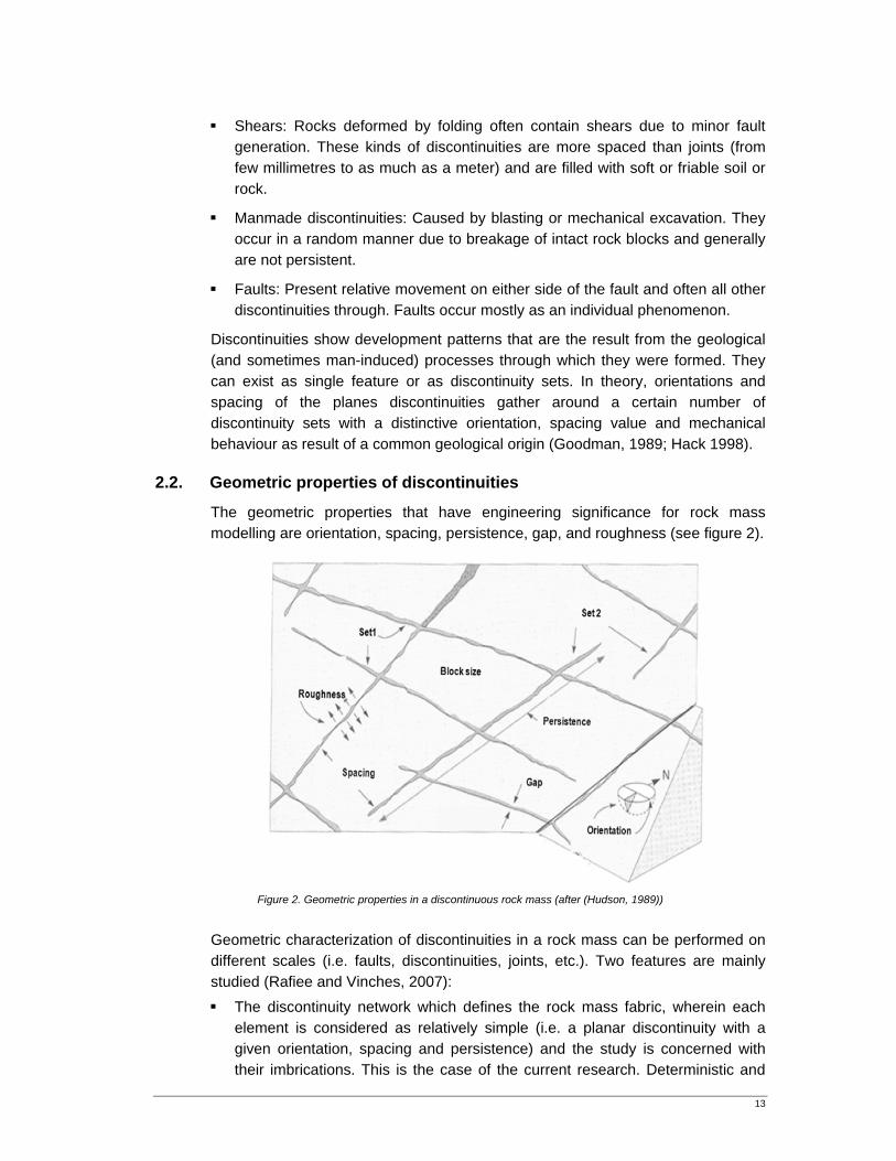
2.2. Geometric properties of discontinuities
The geometric properties that have engineering significance for rock mass modelling are orientation, spacing, persistence, gap, and roughness (see figure 2).
Figure 2. Geometric properties in a discontinuous rock mass (after (Hudson, 1989))
Geometric characterization of discontinuities in a rock mass can be performed on different scales (i.e. faults, discontinuities, joints, etc.). Two features are mainly studied (Rafiee and Vinches, 2007): The discontinuity network which defines the rock mass fabric, wherein each
element is considered as relatively simple (i.e. a planar discontinuity with a given orientation, spacing and persistence) and the study is concerned with their imbrications. This is the case of the current research. Deterministic and
14
statistical methodologies have been used in order to study and model the characteristics of such networks (Billaux et al., 1989a; Chiles, 1989; Ayalew et al., 2002; Kulatilake et al., 2003).
The single discontinuity, which generally does not consist of a pair of simple parallel surfaces. Its study considers roughness characterization on small and large scale, gap, contact areas properties and infill material (Huang et al., 1992; Ehlen, 2000; Yang and Di, 2001; Zillur Rahman, 2005).
The final objective of a geometric characterization is to analyze information provided by field survey data in order to deduce geometric parameters and construct a model of the discontinuity network.
2.3. Traditional methods to collecting discontinuity data
Traditional methods to collecting discontinuity data include scan-line survey, sampling window and rapid face mapping (ISRM, 1981; Kulatilake et al., 1993; La Pointe and Hudson, 1985; Priest, 1993; Priest and Hudson, 1981). Along the present research, scan-line survey and Slope Stability Probability Classification (SSPC) system (Hack, 1998), which is based on a rapid face mapping approach, are used to perform the geometric characterization of the rock mass.
2.3.1. Surface methods
2.3.1.1. Scanline survey
Scanline is a one dimensional discontinuity sampling technique. A line is located on the rock face and discontinuity planes that intersect the scan line are registered with their properties (i.e. location, orientation, trace or semi trace length, persistency, roughness, and infill). A scan-line survey provides statistical information for engineering design purposes; however scan-line is not a standardized method. Additionally, the method can introduce sampling bias in each measured parameter and corrections have to be used to compensate it as is discussed in section 2.6 (ISRM, 1981; Kulatilake et al., 1993; La Pointe and Hudson, 1985; Priest, 1993; Priest and Hudson, 1981).
2.3.1.2. Slope Stability Probability Classification (SSPC) system (Hack, 1998)
In most cases, it is enough to distinguish the principal discontinuity sets and then measure their representative properties (Hack, 1998). First is necessary to identify the most important homogeneous rock mass units and then to carry out the discontinuity sets description for each unit separately. This method has shown to be fast and practical and provides adequate information for most engineering applications. Bias caused by sampling area size and relative orientation as well as under or over-sampling of discontinuities is also avoided. However it does not provide statistical information to determine the variability of the estimated properties. It requires field experience to recognise engineering units and to accurately identify discontinuity sets, hence also human bias may be involved. However, the
15
Slope Stability Probability Classification system provides a systematic approach to perform the rock mass exposure characterization in order to minimize such bias.
2.3.2. Subsurface methods - borehole explorations
Although discussions usually refers to scanline and sampling window data, borehole core logging also provides similar information to that gleaned from a scanline survey (i.e. location, spacing, orientation, roughness and infill) and in fact has shown good correlation (Wines and Lilly, 2002). However, the bias effect due to borehole orientation and the correct identification of actual discontinuities reduce its accurateness. On the other hand it is expensive and an invasive technique.
2.4. Terrestrial Laser Scanner as a recent technique to derive geometric information
As has been stated in the introductory chapter, among other new methodologies such as image analysis and total station, Terrestrial Laser Scanner (hereafter TLS) is a remote sensing technique which has shown a great potential to obtain a large quantity and highly accurate discontinuity geometric information (Slob et al., 2004).
2.4.1. TLS fundamentals
During a TLS survey, a laser beam emits repeated pulses that are reflected by the rock face. These measurements can be translated into xyz-coordinates, using either the two way time of flight for each received pulse or the amplitude modulated continuous wave principle (Fröhlich, 2004). This results in the acquisition of a dense 3D point cloud of the rock surface with a high spatial resolution (5 – 10 mm), which represents the surface shape at a very high detail (see figure 3). The xyz data can be complemented with the intensity value of each returned pulse and color information extracted from digital imagery (Slob and van Knapen, 2006). There are a number of 3D laser scanning devices on the market that use the ranging principle, (i.e. Leica-Cyrax, Riegl, Trimble-Mensi). Their principles are the same, but the quality attributes of the data (i.e. resolution, accuracy, precision, scanning speed, and laser beam divergence) may vary between manufacturers and models. Further details can be found in (Fröhlich, 2004).
2.4.2. Data processing
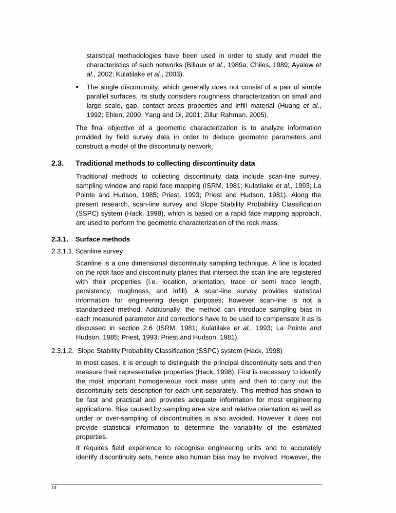
Prior to realize the geometric analysis, TLS data must be reoriented with respect to the true north. This can be achieved a) using control points on the rock face with known x, y and z coordinates, b) knowing the true orientation (respect to the north) of at least two control surfaces on the rock face (usually control boards) or c) knowing the true orientation of the laser scanner (Slob et al., 2005). TLS data provide a very good visual impression of the scanned object (see figure 3). However, further analysis is required to construct a true 3D surface model; this can be followed through two methodologies as follows:
2.4.2.1. Proc
ThisdataPolypolyspaby aTheparaFunWhof tpresmovrecoorierecoroun
2.4.2.2. Dire
ThisfacerecobeloTheneigvericlasseleto tpoin
cessing thro
s methodoloa. Reconstrygonal technygonal patch
ace (Kemenya number ofe continuouametric tec
nctions (Carrile creating tthe laser sesence of forvement) whonstruction i
entations of tonstruction nded edges
Figure 3.
ect segmenta
s approach we and henceognised andong to a parte method stghboring pofied that mo
ssified with ected and it he same plants are found
ough surface
ogy is baseduction algorniques (i.e. Dhes based oy and Donovf parametric us surface chniques arer et al., 2003the surface,ettings, its rreign objectsich affect this influencedthe trianglesmethods cathat are act
. a) Rock mass s (
ation (Slob e
works undere also in the d defined andticular planearts with the
oints are chost of the nei
a label. Frois again detane that wad, which dem
e reconstruct
d on the crerithms can bDelaunay anon simple linvan, 2005). P
surface patis then cr
e Non-Unifo3; Carr et al., sparse reg
relative ories (i.e. vegethe correctned by the nos can be affean produce bually sharp.
scanned surface,(Slob and van Kn
et al., 2006)
r the assumpoint cloud d the point c
e (see figure e selection osen withinighboring poom these laermined whe
as found befmarcates the
tion (Slob et
eation of a be divided nd Voronoi tenear interpoParametric tetches descrireated by jorm Ration, 2001). Seeions in the pntation withation) or dy
ess of the reise present
ected as welblobby shap
, b) Polygonal sunapen, 2006)
ption that fladata. Througcloud is clas4). of a seed p a specified
oints lie closeabeled pointether most ofore. This pre end of the
t al., 2005).
3D structurinto Polygonetrahedrisatlation betweechniques rebed by mathjoining patc
nal B-Splinee figure 3. point cloud ch respect tonamic distu
econstructedin the data,l. On the oth
pes in such
urface reconstruc
at planes aregh the proce
ssified into s
point aroundd search dise to the samts, their neiof these poinrocess is reconstruction
e in the ponal and Partion) create ieen the poinepresent thehematical eqches. Exames or Radia
can appear o the rock frbances (i.ed surface. P, then the coher hand, pasparse regi
ction
e present in ess these plaubsets of po
d which thestance. If it
me plane, theghboring ponts are locatpeated untiln of a plane.
int cloud rametric. irregular, nts in 3D e surface quations. mples of al Basis
because face, the e. ground Polygonal omputed arametric ions and
the rock anes are oints that
e nearest t can be ey are all oints are ted close l no new . Then, a
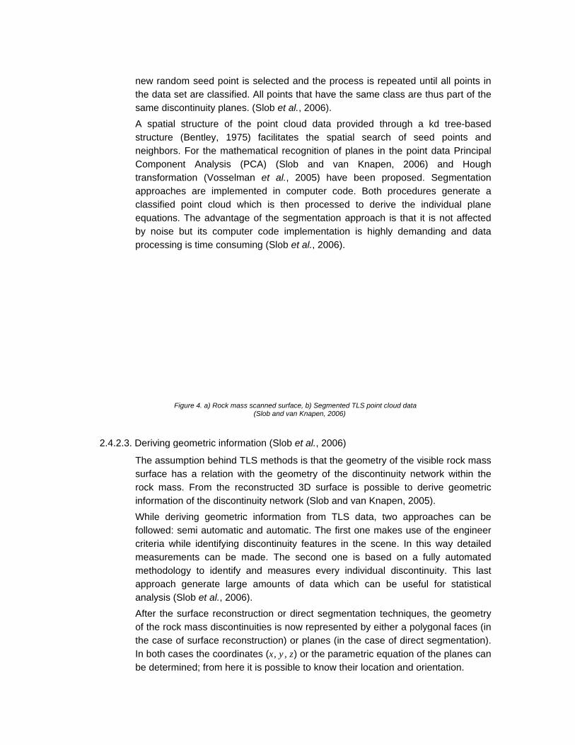
2.4.2.3
new randthe data ssame discA spatial structure neighborsComponetransformapproachclassified equationsby noise processin
F
3. Deriving g
The assumsurface hrock masinformatioWhile defollowed: criteria wmeasuremmethodoloapproach analysis (After the of the rocthe case oIn both cabe determ
om seed poset are classcontinuity pla
structure o(Bentley,
s. For the ment Analysisation (Vosses are imppoint cloud
s. The advanbut its com
ng is time co
Figure 4. a) Rock
geometric inf
mption behinhas a relatioss. From theon of the discriving geomsemi automhile identifyments can bogy to iden
generate lSlob et al., 2surface reco
ck mass discof surface re
ases the coomined; from h
oint is selectsified. All poanes. (Slobof the point1975) facili
mathematicals (PCA) (selman et alemented ind which is ntage of the
mputer codensuming (Sl
k mass scanned (Slob an
formation (S
nd TLS methon with the ge reconstruccontinuity ne
metric informmatic and au
ing discontinbe made. Tntify and melarge amou2006). onstruction
continuities iseconstructioordinates (x, here it is pos
ted and the ints that havet al., 2006)t cloud datatates the sl recognition(Slob and al., 2005) hn computer then proce
e segmentate implementob et al., 20
surface, b) Segmnd van Knapen,
Slob et al., 20
hods is that geometry ofcted 3D suretwork (Slob
mation from tomatic. Thenuity feature
The second easures events of data
or direct ses now repre
on) or planes y, z) or the ssible to kno
process is rve the same). a provided spatial searn of planes i
van Knaphave been
code. Bothessed to detion approactation is hig06).
mented TLS poin2006)
006)
the geometf the disconrface is posb and van Kn
TLS data,e first one mes in the scone is bas
ery individuaa which can
gmentation sented by es (in the casparametric e
ow their loca
repeated une class are th
through a rch of seein the point pen, 2006)
proposed. h procedureerive the indch is that it ghly demand
nt cloud data
ry of the visntinuity netwssible to dernapen, 2005
two approamakes use ocene. In thissed on a fual discontin
n be useful
techniques,either a polygse of direct sequation of ttion and orie
ntil all pointshus part of t
kd tree-basd points adata Princip
and HouSegmentati
es generatedividual plais not affectding and da
ible rock mawork within trive geomet
5). aches can
of the engines way detailully automatuity. This lafor statistic
the geomegonal faces segmentatiothe planes centation.
in the
sed and pal
ugh on
e a ane ted ata
ass the tric
be eer ed
ted ast cal
etry (in n).
can
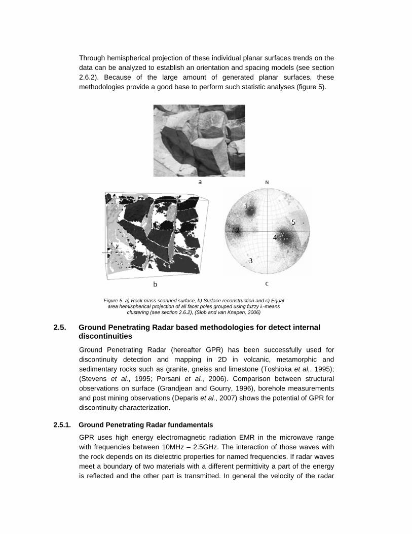
Throdata2.6.met
2.5. Grodisc
Grodiscsed(Steobsanddisc
2.5.1. Gro
GPRwiththe meeis re
ough hemisa can be an.2). Becausthodologies
Figure 5. aarea hem
ound Penecontinuitie
ound Penetrcontinuity dimentary roc
evens et alservations ond post miningcontinuity ch
ound Penetr
R uses highh frequencierock depend
et a boundaeflected and
pherical projalyzed to es
se of the provide a go
a) Rock mass scmispherical projeclustering (see s
trating Rades
rating Radadetection ancks such asl., 1995; Pon surface (Gg observatioharacterizatio
rating Rada
h energy elees between ds on its die
ary of two mad the other p
jection of thstablish an olarge amouood base to
canned surface, bection of all facet section 2.6.2), (S
dar based
ar (hereaftend mappings granite, gnorsani et aGrandjean ans (Deparison.
ar fundamen
ectromagne10MHz – 2.
electric propeaterials withpart is trans
ese individuorientation aunt of geneperform suc
b) Surface recont poles grouped uSlob and van Kna
methodolo
r GPR) hag in 2D inneiss and liml., 2006). C
and Gourry, et al., 2007
ntals
tic radiation5GHz. The erties for namh a different smitted. In g
ual planar sund spacing erated planch statistic a
struction and c) using fuzzy k-meapen, 2006)
ogies for d
as been sun volcanic,
mestone (ToComparison 1996), bore) shows the
n EMR in thinteraction med frequenpermittivity
general the v
urfaces trendmodels (see
nar surfacesnalyses (figu
Equal eans
detect inter
ccessfully umetamorp
oshioka et albetween s
ehole measupotential of
he microwavof those wancies. If radaa part of thevelocity of t
ds on the e section s, these ure 5).
rnal
used for phic and l., 1995); structural urements GPR for
ve range aves with ar waves e energy he radar
19
wave in a material varies with its dielectric permittivity and attenuation increase with increasing frequencies (therefore with increasing wavelength as well). GPR equipment consists principally of a control unit, a transmitter and a receiver. A computer is used for data collection. The transmitters and the antennas of transmitter and receiver can be changed to operate the GPR at different frequencies. The transmitter generates a single and short high voltage pulse and transmits it into the antenna, which emits EMR of a specific frequency into the surrounding area. The receiver collects incoming signals in samples which are a digital representation of the amplitude and phase of the signac3ar6l in a certain unit of time. To improve ratio between signal and noise, several samples are recorded simultaneously and are put together to a so called stack by calculating their mean value. Transmitter and receiver can be placed in fixed configurations such as monostatic, bistatic, mobile or common middle point. The selection of the configuration depends on the specific conditions of the survey. A full theoretical basis of GPR can be found in (Davis and Annan, 1989; Parasnis, 1997; Reynolds, 1997).
2.5.2. Ground Penetrating Radar as a technique to detect internal discontinuities
When compared with other traditional subsurface exploration methods such as borehole (see section 2.3.2), GPR has demonstrated to be a suitable geophysical method to detect internals discontinuities in a rock mass. Depending on the survey requirements, it can reach the required vertical and horizontal resolution and depth penetration. Additionally it is a non destructive method and GPR surveys are usually fast and economical (Deparis et al., 2007; Grandjean and Gourry, 1996) Literature shows that the feasibility of GPR technique is limited by a) the degree of discontinuity detection, b) the penetration versus resolution radio and c) the complexity of the discontinuity network as follows (Grandjean and Gourry, 1996): Degree of discontinuity detection
There is a minimal aperture for a discontinuity to be detected by GPR, according to the filling material in the discontinuity, the propagating medium and the frequency acquisition (Deparis and Garambois, 2006). Depending on the electrical properties of the rock and the infill material (electric conductivity and dielectric permittivity) the amount of returned energy can be high. In such way different resolutions and penetration depths can be reached (Grandjean and Gourry, 1996). Penetration versus resolution
It is important to note that GPR is unable to distinguish discontinuities separated by a distance lower than a half-wavelength (Reynolds, 1997). The main difficulty in discontinuity detection is the ambiguous relation between penetration depth and resolution. The higher the signal frequency the better the resolution is. In the other hand the higher the frequency, the higher the attenuation is. This is because of the increasing attenuation of the propagating GPR wave at higher frequencies. However, depending on the electrical properties of the rock, attenuation can be low.
20
Complexity of the discontinuity network
Discontinuities can be correctly detected and located on condition that they are sufficiently opened and separated from each other; otherwise they can create a complex reflectivity pattern and cannot be distinguished anymore. Multi-reflections and 3D geometric effects can be also possible in discontinuities with a roughness of strong amplitude. Ideally, a complete determination of the discontinuities would require a set of close parallel and perpendicular GPR profiles as well as compound processing and interpretation methodology (Deparis et al., 2007). Finally a representation of the discontinuity network can be obtained through the correlation of discontinuity signatures of each profile with those from the nearest one (Grandjean and Gourry, 1996).
2.5.3. GPR data processing methodology
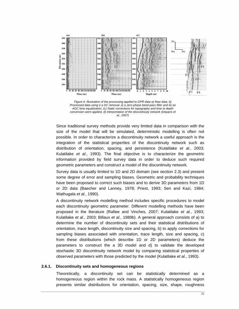
The objective of the processing is to enhance the reflected and diffracted signal returned from the discontinuities. A standard processing methodology includes amplitude compensation, filtering, migration, static correction, display and interpretation (Reynolds, 1997). In this way the diffractors and reflectors can be located accurately and the signal profile becomes clearer. The processed intensity values are converted and displayed as signal voltage versus two-way time. In one type of display the intensity is plotted as wiggle curve with the positive area in each wiggle blacked. Other case is the variable-area display where successive scans at points along the profile are plotted side by side. (Reynolds, 1997). Interpretation of the obtained profiles is based on the assumption that reflection horizons and refraction bright spots correspond to discontinuities and cavities in the rock. Interpretation must be performed and validated by gathering of available information (see figure 6).
2.6. Discontinuity network modelling
As was stated before in section 2.2, the discontinuity network modelling is concerned with the imbrications of the different discontinuities wherein each one of these elements is considered as relatively simple: a planar surface with a given orientation, spacing and persistence. Discontinuity network modelling must be tailored to end use requirements (i.e. kinematics analysis of mechanical stability, discrete analysis of a blocky rock mass, or statistic characterization of geometric parameters). In general, the discontinuity network can be treated either by a deterministic model where discontinuities are considered separately as single features (which geometric properties are all known) or by a stochastic model (where geometric properties of the discontinuities are statistically inferred) (Kulatilake et al., 1993).
21
Figure 6. Illustration of the processing applied to GPR data a) Raw data, b)
Processed data using i) a DC removal ,ii) a zero-phase band-pass filter and iii) an AGC time equalization. (c) Static corrections for topography and time to depth
conversion were applied, d) Interpretation of the discontinuity network (Deparis et al., 2007)
Since traditional survey methods provide very limited data in comparison with the size of the model that will be simulated, deterministic modelling is often not possible. In order to characterize a discontinuity network a useful approach is the integration of the statistical properties of the discontinuity network such as distribution of orientation, spacing, and persistence (Kulatilake et al., 2003; Kulatilake et al., 1993). The final objective is to characterize the geometric information provided by field survey data in order to deduce such required geometric parameters and construct a model of the discontinuity network. Survey data is usually limited to 1D and 2D domain (see section 2.3) and present some degree of error and sampling biases. Geometric and probability techniques have been proposed to correct such biases and to derive 3D parameters from 1D or 2D data (Baecher and Lanney, 1978; Priest, 1993; Sen and Kazi, 1984; Wathugala et al., 1990). A discontinuity network modelling method includes specific procedures to model each discontinuity geometric parameter. Different modelling methods have been proposed in the literature (Rafiee and Vinches, 2007; Kulatilake et al., 1993; Kulatilake et al., 2003; Billaux et al., 1989b). A general approach consists of a) to determine the number of discontinuity sets and their statistical distributions of orientation, trace length, discontinuity size and spacing, b) to apply corrections for sampling biases associated with orientation, trace length, size and spacing, c) from these distributions (which describe 1D or 2D parameters) deduce the parameters to construct the a 3D model and d) to validate the developed stochastic 3D discontinuity network model by comparing statistical properties of observed parameters with those predicted by the model (Kulatilake et al., 1993).
2.6.1. Discontinuity sets and homogeneous regions
Theoretically, a discontinuity set can be statistically determined as a homogeneous region within the rock mass. A statistically homogeneous region presents similar distributions for orientation, spacing, size, shape, roughness
22
intensity and constitutive properties; however as is discussed in section 2.6.2. However, in practice only the number of discontinuity sets and its orientation distribution are considered in determining statistically homogeneous regions (Kulatilake et al., 2003; Kulatilake et al., 1993).
2.6.2. Discontinuity orientation
2.6.2.1. Data acquisition
Orientation data acquisition routines are part of traditional techniques for geometric characterization of discontinuities based on the interpretation of the visible surface of a rock mass outcrop include one dimensional scan line survey, two dimensional mapping, borehole exploration and rapid face mapping using a field form to systematically direct the mapping of a rock face (see section 2.5). Recent remote sensing based techniques include digital image analysis (Kemeny, 2003), digital photogrammetry (Roncella and Forlani, 2005) and photo total station (Zhang et al., 2004). As was discussed in section 2.4 terrestrial laser scanner has shown a great potential to obtain a large quantity and highly accurate discontinuity geometric information (Slob et al., 2004).
2.6.2.2. Discontinuity orientation representation
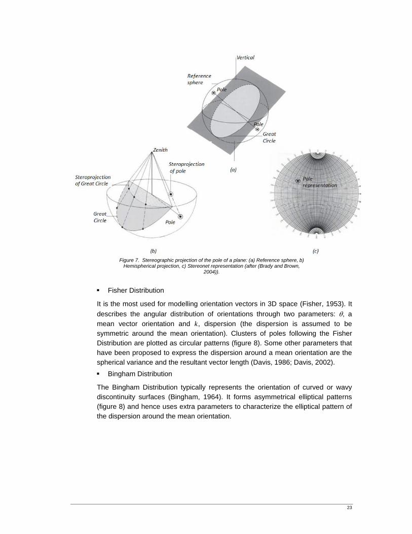
The graphic representation of discontinuity orientation and the recognition of statistical homogeneous regions (discontinuity sets) are usually performed using techniques of hemispherical projection of discontinuity poles (Priest, 1985; Priest, 1993). The hemispherical projection is a method of representing and analyzing the three-dimensional relations between planes on a two dimensional projection plane using a reference sphere (see figure 7). Details about the steps required to construct a hemispherical projection using a stereonet can be found in (Brady and Brown, 2004). Engineering applications are described in detail by (Goodman, 1989; Goodman and Shi, 1985), (Hoek and Bray, 1981), (Priest, 1985; Priest, 1993). It becomes useful to use the representation of the planes in the form of poles when dealing with large volumes of orientation data. This is also helpful in identifying statistically homogeneous regions. Poles to discontinuity planes that have a similar orientation (parallel planes) will plot as distinct clusters.
2.6.2.3. Orientation homogeneity modelling
Several techniques have been proposed in order to identify clusters of similar discontinuity orientations using graphical analysis of the poles in a hemispherical projection (Hoek and Bray, 1981; Priest, 1993). These clusters exhibit specific distribution characters called orientation models. The most commonly used are:
23
Figure 7. Stereographic projection of the pole of a plane: (a) Reference sphere, b)
Hemispherical projection, c) Stereonet representation (after (Brady and Brown, 2004)).
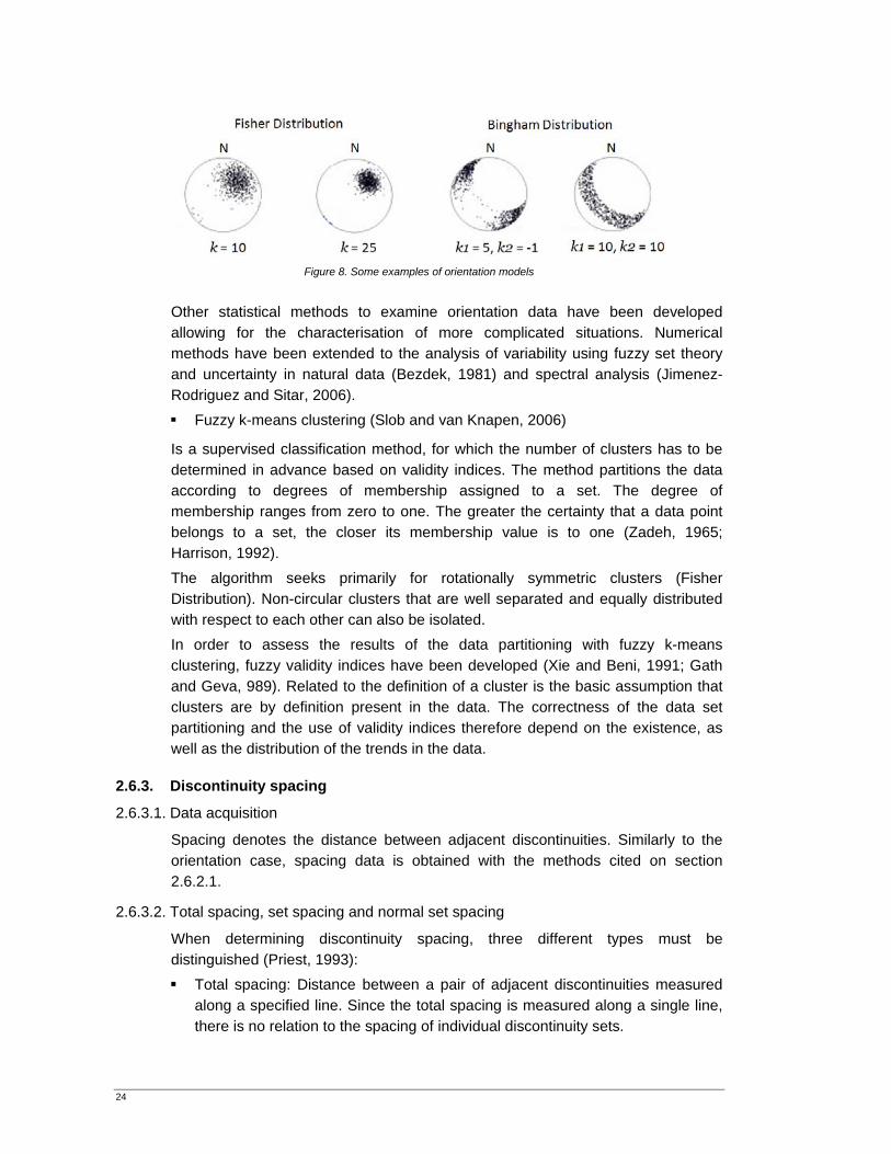
Fisher Distribution
It is the most used for modelling orientation vectors in 3D space (Fisher, 1953). It describes the angular distribution of orientations through two parameters: θ, a mean vector orientation and k, dispersion (the dispersion is assumed to be symmetric around the mean orientation). Clusters of poles following the Fisher Distribution are plotted as circular patterns (figure 8). Some other parameters that have been proposed to express the dispersion around a mean orientation are the spherical variance and the resultant vector length (Davis, 1986; Davis, 2002). Bingham Distribution
The Bingham Distribution typically represents the orientation of curved or wavy discontinuity surfaces (Bingham, 1964). It forms asymmetrical elliptical patterns (figure 8) and hence uses extra parameters to characterize the elliptical pattern of the dispersion around the mean orientation.
24
Figure 8. Some examples of orientation models
Other statistical methods to examine orientation data have been developed allowing for the characterisation of more complicated situations. Numerical methods have been extended to the analysis of variability using fuzzy set theory and uncertainty in natural data (Bezdek, 1981) and spectral analysis (Jimenez-Rodriguez and Sitar, 2006). Fuzzy k-means clustering (Slob and van Knapen, 2006)
Is a supervised classification method, for which the number of clusters has to be determined in advance based on validity indices. The method partitions the data according to degrees of membership assigned to a set. The degree of membership ranges from zero to one. The greater the certainty that a data point belongs to a set, the closer its membership value is to one (Zadeh, 1965; Harrison, 1992). The algorithm seeks primarily for rotationally symmetric clusters (Fisher Distribution). Non-circular clusters that are well separated and equally distributed with respect to each other can also be isolated. In order to assess the results of the data partitioning with fuzzy k-means clustering, fuzzy validity indices have been developed (Xie and Beni, 1991; Gath and Geva, 989). Related to the definition of a cluster is the basic assumption that clusters are by definition present in the data. The correctness of the data set partitioning and the use of validity indices therefore depend on the existence, as well as the distribution of the trends in the data.
2.6.3. Discontinuity spacing
2.6.3.1. Data acquisition
Spacing denotes the distance between adjacent discontinuities. Similarly to the orientation case, spacing data is obtained with the methods cited on section 2.6.2.1.
2.6.3.2. Total spacing, set spacing and normal set spacing
When determining discontinuity spacing, three different types must be distinguished (Priest, 1993): Total spacing: Distance between a pair of adjacent discontinuities measured
along a specified line. Since the total spacing is measured along a single line, there is no relation to the spacing of individual discontinuity sets.
25
Set spacing: Distance between a pair of adjacent discontinuities belonging to the same set, along a specified line. The average of all set spacings is the mean set spacing. There is no correction for the orientation of the scanline. In consequence, the spacing for a set that is oriented almost parallel to the scanline is greatly over estimated.
Normal set spacing: Distance between a pair of adjacent discontinuities, from the same set, perpendicular to the average orientation in that set. The average of all normal set spacings is the mean normal set spacing. Normal set spacing and mean normal set spacing are good indicators of the block shape and size distribution in the rock mass.
2.6.3.3. Sampling bias correction
The estimation of mean spacing and frequency (1/spacing) is based on the measurements carried out on finite length scan-lines in single and different orientations; hence an orientation correction must be performed in order to derive correct values for normal set spacing. Methods proposed to compensate such biases are proposed in (Kulatilake et al., 1993; La Pointe and Hudson, 1985).
2.6.3.4. Discontinuity spacing and frequency modelling
Discontinuity spacing behaviour is usually treated using statistical methods based on the central limit theorem (Priest and Hudson, 1981). The inverse of the mean spacing is the mean frequency of intersections along the scanline and the frequency of occurrence of the discontinuity spacing varies within a series of spacing ranges and can be represented by some probability distribution (either for individual discontinuity sets or for all discontinuity data). (Priest, 1985) described and illustrated the difference between Negative exponential, Uniform and Normal distributions of spacing. However, it has been shown that discontinuity sets can follow a Lognormal or Fractal distribution (Hobbs, 1993). Weibull or Negative exponential distributions can be also applicable. (Kulatilake et al., 1993) also mentioned the Gamma distribution to describe the distribution of discontinuity spacing. Goodness of fit tests must to be performed to find a suitable probability distribution as well as the best probability distribution to represent the statistical distribution of spacing for each discontinuity set obtained from data (Kulatilake et al., 2003).
2.6.4. Trace length and persistence
2.6.4.1. Trace length sampling
Trace length describes the prolongation of a discontinuity in a given orientation (Priest and Hudson, 1981). Since predominantly only a single trace or a part of the discontinuity is exposed in a rock face, to determine actual trace length of the discontinuities in a rock mass is difficult. A fair approach is to measure or estimate the trace length of the discontinuity along dip and along strike, in this way two dimensional persistence can be derived (Hack, 1998). Information about trace length is derived from traditional survey methods (section 2.3).
26
For each discontinuity set, the semi-trace length data can be analyzed under three categories: (a) data above (in the case of a horizontal scanline) or to the right of scanline (in the case of a vertical scanline); (b) data below (in the case of a horizontal scanline) or to the left of scanline (in the case of a vertical scanline); and (c) data on both sides of the scanline (Kulatilake et al., 2003).
2.6.4.2. Sampling bias correction
Observed trace lengths sampled on finite size exposures are subject to size censoring and truncation biases. Effect of censoring and truncation bias causes that the estimated trace length and its statistical distribution differs from the actual one. Bias correction must be also performed for this reason (Kulatilake, 1985; Priest and Hudson, 1981). Once the corrected mean trace length is estimated from censored semi-trace lengths through this procedure, it is then possible to establish the trace length distribution with the estimated corrected mean trace length.
2.6.4.3. Trace length modelling
Similarly to spacing statistics, trace length is also usually treated using statistical methods based on the central limit theorem. Goodness of fit tests to check the suitability of exponential, gamma, lognormal and normal distributions have been discussed by (Ang and Tang, 1975) and (Benjamin and Cornell, 1970). According to literature usually either the lognormal or the exponential distribution are the most suitable to describe the trace length statistical distribution. (Robertson, 1970) concluded that the strike and dip trace lengths have about the same distribution (implying discontinuities are equidimensional), however some studies have shown that this is not necessarily always true (Bridges, 1975).
2.6.4.4. Persistence
In statistical terms, persistence (prolongation of the trace length of a discontinuity in a given direction) can be defined as the probability that any discontinuity cuts a block that lies in its path (Kalenchuk et al., 2006; Einstein, 1993). This parameter can be seen as an alternative parameter for trace length. Persistence can have a value between 0 and 1. For a value near to 1, there would be more discontinuities that go through other discontinuities. For values near to 0, a given discontinuity end when intersecting other ones. In practice the persistence value for each discontinuity set is determined comparing the discontinuity length distribution obtained from the field survey with the distribution resulting from the generated model.
2.7. Discontinuity network modelling and validation
To describe the discontinuity network geometry in 3D for a homogeneous rock mass model, it is necessary to specify the distributions that are obtained for orientation; spacing, trace length and persistence (see section 2.6). From those parameters, further analyses (which are out of the scope of this research) would permit to generate a virtual discontinuity network in 3D which is used to make predictions from a virtual scanline or a virtual sampling window. A comparison
27
between the distributions of the geometric parameters derived from such virtual scanline with those observed in the rock mass permit to validate the model. Further details can be found on (Billaux et al., 1989b; Kulatilake et al., 2003).
3. Methodology
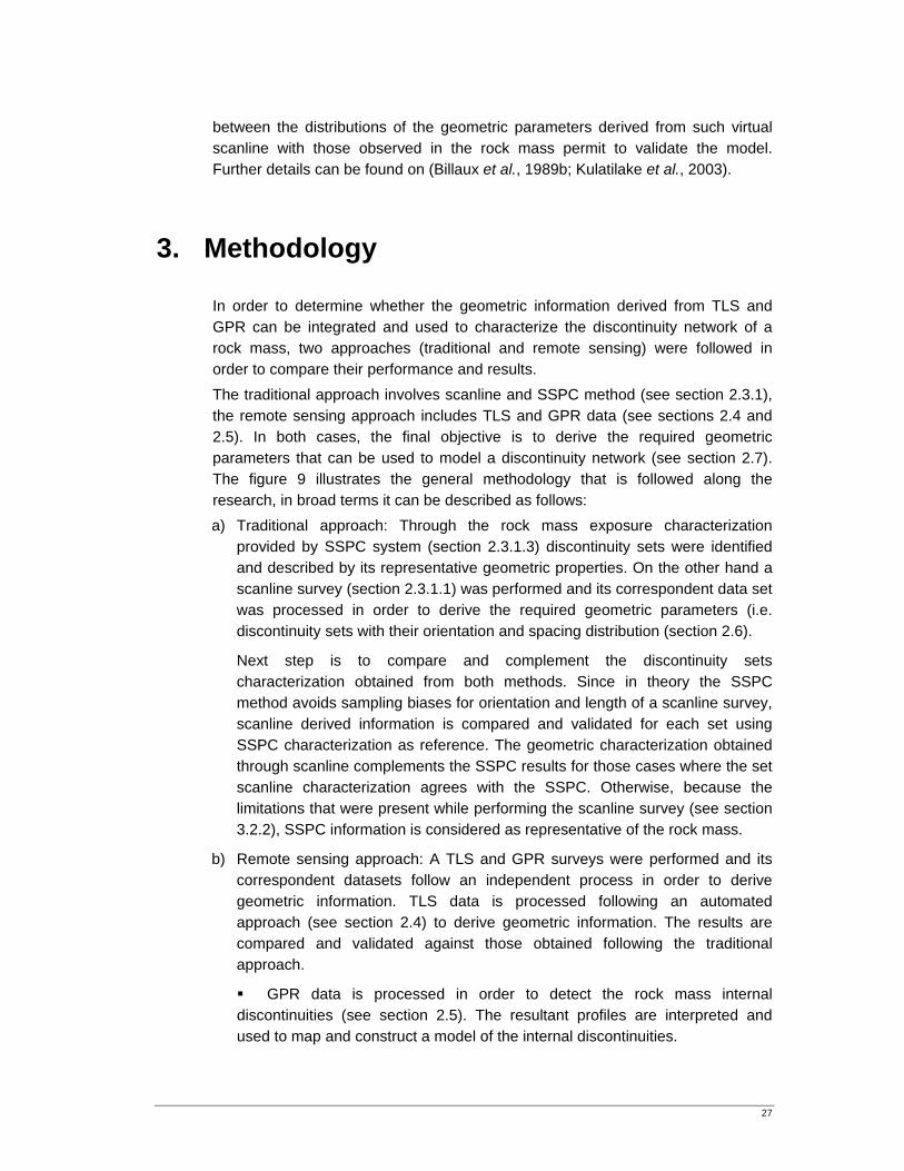
In order to determine whether the geometric information derived from TLS and GPR can be integrated and used to characterize the discontinuity network of a rock mass, two approaches (traditional and remote sensing) were followed in order to compare their performance and results. The traditional approach involves scanline and SSPC method (see section 2.3.1), the remote sensing approach includes TLS and GPR data (see sections 2.4 and 2.5). In both cases, the final objective is to derive the required geometric parameters that can be used to model a discontinuity network (see section 2.7). The figure 9 illustrates the general methodology that is followed along the research, in broad terms it can be described as follows: a) Traditional approach: Through the rock mass exposure characterization
provided by SSPC system (section 2.3.1.3) discontinuity sets were identified and described by its representative geometric properties. On the other hand a scanline survey (section 2.3.1.1) was performed and its correspondent data set was processed in order to derive the required geometric parameters (i.e. discontinuity sets with their orientation and spacing distribution (section 2.6).
Next step is to compare and complement the discontinuity sets characterization obtained from both methods. Since in theory the SSPC method avoids sampling biases for orientation and length of a scanline survey, scanline derived information is compared and validated for each set using SSPC characterization as reference. The geometric characterization obtained through scanline complements the SSPC results for those cases where the set scanline characterization agrees with the SSPC. Otherwise, because the limitations that were present while performing the scanline survey (see section 3.2.2), SSPC information is considered as representative of the rock mass.
b) Remote sensing approach: A TLS and GPR surveys were performed and its correspondent datasets follow an independent process in order to derive geometric information. TLS data is processed following an automated approach (see section 2.4) to derive geometric information. The results are compared and validated against those obtained following the traditional approach.
GPR data is processed in order to detect the rock mass internal discontinuities (see section 2.5). The resultant profiles are interpreted and used to map and construct a model of the internal discontinuities.
28
After validating geometric characterization provided by TLS method with SSPC characterization as reference, both TLS and GPR derived geometric information is complemented to generate a final model. This model is validated again against the results of the traditional approach.
In all the cases validation is performed for each discontinuity set by comparison of the derived geometric parameters and their statistical characteristics (when possible).
Figure 9. General methodology flowchart
3.1. Study site
A single rock mass exposure located in a porphyry quarry at Albiano (Province of Trento, North Italy) was chosen to perform the field data acquisition. Porphyry stone has become one of the most important materials for paving and facing in Europe and it is intensively mined in several quarries at the area. The porphyry stone correspond to a Permian rhyolite present on the so called “Atesine Porphyric Platform”, a result of alternate eruptive and stable phases started 260 million years ago. Figure 10 shows both location and geological setting of the study site. Data acquisition was performed on 13 September, 2007.
3.2.
Figu
Weather
At the molevel at thare well aand no wain the nigprobably discontinu
ure 10. Study sit(Pe
r, seepage
oment of the he sites was above quarryater seepag
ght water main intact ro
uity infill mat
te at Albiano (Proermian Rhyolite),
groundwa
field campabelow the q
y bottom. It he has been ay have conock. Henceterial is dam
Tr
ovince of Trento, b) Location, c) g
ater conditi
aign the rockquarry bottomhas not beennoticed on t
ndensed ande, it cannotp or wet dur
Stud
Stud
Trento
Trento
North Italy) a) Pgeological map
ions
k mass was m whereas tn raining durthe investigad seeped int be excludring the inves
dy Site
dy Site
Alb
Albia
Porphyry quarry
dry. The pehe investigaring the perioated exposunto the discoded that intstigations.
biano
no
rmanent waated exposurod of fieldwo
ures. Howevontinuities atact rock a
ter res ork er,
and and
30
3.3. Geometric characterization, traditional approach
3.3.1. Slope Stability Probability Classification (SSPC)
The objective of the SSPC system (Hack, 1998) is to get generalised geometric information for the rock mass exposure (number of sets with their orientation, normal set spacing and persistence).
3.3.1.1. Field method
The characterization of the discontinuity sets and the measurement of the discontinuity parameters in the SSPC method are based on the rapid face mapping approach (section 2.3.1.3), it includes the description of the rock mass according to Code of Practice for Site Investigations (British Standard Institution, 1999).
3.3.1.2. Limitations
Rapid face mapping based methods present human bias when determining representative parameters (see section 2.3.1.3). On the other hand instrument errors can be also involved.
3.3.1.3. Results
According to the BS classification system (BS 5930; 1999) the rock can be described as: Grey, Coarse crystalline size, Foliated large tabular, Fresh - slightly weathered RHYOLITE. Field form and its details are presented in appendix 1.
Figure 11. Rock mass exposure at Albiano quarry (Permian Rhyolite), height ≈ 20m.
Six discontinuity sets were identified while using the SSPC system (see table 1). The geometric characterization of such sets is based on the rapid face mapping approach (see section 2.3.1.3).
31
Set / Parameter J1 J2 J3 J4 J5 J6
Dip direction (°) 170 248 268 250 280 080
Dip angle (°) 86 80 82 52 05 55
Normal set spacing (m) 0.07 1.00 1.00 4.00 2.00 5.00
Persistence (Along Strike) > > 0.07 0.50 > 10.00
Persistence (Along Dip) > > 3.00 0.50 > 0.20
Table 1. SSPC rock mass geometric description ( > denotes greater than the exposure size, see SSPC filed form details in appendix 1)
3.3.2. Scanline Survey
Since the SSPC system gives a generalised characterization of the rock exposure, the objective of the scanline survey is to acquire geometric data in a systematic way in order to complement the information derived from SSPC.
3.3.2.1. Field Methods
The scanline survey was performed according to the method suggested by (Windsor and Robertson, 1994)). Three horizontal scanline surveys were preformed on the rock exposure (see appendix 2). A total of 19.80 m of scanline were mapped for a total of 35 discontinuity measurements and the orientation of the scanline relative to the orientation of the main discontinuity sets was chosen in order to minimize sampling bias (see figure 12).
Figure 12. Scanline survey
3.3.2.2. Limitations
Similarly to the SSPC method, scanline surveys involve both human bias and error in measurements when determining representative geometric parameters. Additional to these facts the following drawbacks in the survey were noted in the context of this study:
32
Since SSPC method determined the presence of a sub-horizontal discontinuity set (see table 1), it would have been necessary to perform a vertical mapping, however, due to time constraints it was not possible to perform it.
Even though pre-splitting is used along most quarry walls, the exposure exhibits some degree of local damage (see appendix 1). Special care had to be taken in order to avoid recording such cracks as discontinuities, but this fact also implies human bias while doing the survey.
According to the SSPC characterization, some of the discontinuity sets exhibit a representative set spacing up to five meters (see table 1). (Priest and Hudson, 1981) suggested a scanline length of at least 50 times the mean discontinuity set spacing in order to provide an ideal representation of the properties of each set. This condition can not be achieved for all discontinuity sets.
Bias produced by scanline length and orientation limited the usefulness of the scanline method. In general it was found that the sample size for each set is too small to statistically state conclusions. Despite of this, fuzzy k-means clustering was applied to orientation data (see section 2.6.2.4) in order to split the data into clusters. This permitted to reach some agreement with the SSPC observations and estimate the geometric parameters.
3.3.2.3. Results
Table 2 presents the results of the scanline survey method after orientation correction (see computation details in appendix 2). Through hemispherical projection of orientation data (see section 2.6.2.3) and fuzzy k-means clustering, five discontinuity sets can be recognised (see figure 13). According to section 2.6.2 and 2.6.3, for each identified set the mean orientation, resultant vector R, Fisher k constant, spherical variance s, and normal mean spacing were calculated. Regardless of the described limitations, the scanline and the SSPC results correlate reasonably well. This is discussed in detail in the next section.
Cluster / Parameter 1 2 3 4 5 6
Mean dip direction (°) 175 254 266 255 - 81
Mean dip angle (°) 85 89 81 57 - 64
Sample Size N 6 10 5 10 - 4
Resultant vector R 6.00 6.01 4.99 9.87 - 4.97
Fisher k constant 9436* 184.0 338.4* 436.1 - 179.2*
Spherical variance s 0 0.399 0.002 0.013 - 0.005
Mean normal set spacing (m) 0.06 0.83 0.77 1.52 - 0.48
Std. deviation normal set spacing (m) 0.01 0.80 0.61 1.18 - 0.35
Max. normal set spacing (m) 0.08 2.48 1.80 2.81 - 0.73
Min. normal set spacing (m) 0.06 0.20 0.20 0.51 - 0.24
Table 2. Descriptive statistics of the scanline surveys results (* Fisher k constant is not valid if the sample size N is smaller than 10)
3.3.3.
Set / Cluster
1
2
3
4
5
6
Considlimitat
Validation
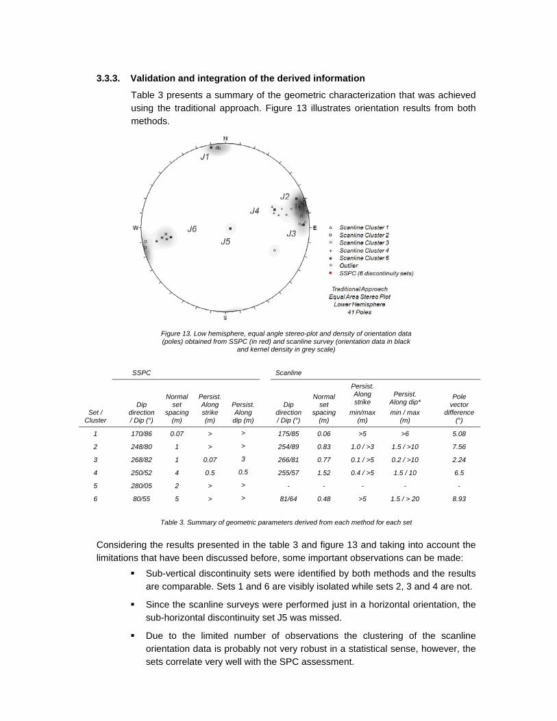
Table 3 pusing themethods.
Fig(po
SSPC
Dip direction / Dip (°)
N
sp
170/86
248/80
268/82
250/52
280/05
80/55
Tab
dering the reions that hav
Sub-vare co
Since sub-ho
Due torientasets c
n and integ
presents a s traditional
ure 13. Low hemoles) obtained fro
Normal set
pacing (m)
PersistAlong strike (m)
0.07 >
1 >
1 0.07
4 0.5
2 >
5 >
ble 3. Summary o
esults preseve been discertical disco
omparable. S
the scanlineorizontal dis
to the limiteation data isorrelate very
ration of th
ummary of tapproach. F
misphere, equal aom SSPC (in red)
and kernel
t. Persist. Along
dip (m)
>
>
3
0.5
>
>
of geometric para
ented in the cussed befoontinuity setsSets 1 and 6
e surveys wcontinuity se
ed number s probably ny well with th
e derived in
the geometrFigure 13 ill
angle stereo-plot d) and scanline sul density in grey s
Scanline
Dip direction / Dip (°)
N
sp
175/85
254/89
266/81
255/57
-
81/64
ameters derived
table 3 and re, some ims were ident6 are visibly i
were performet J5 was m
of observaot very robuhe SPC asse
nformation
ric characterustrates orie
t and density of ourvey (orientationscale)
Normal set
pacing (m)
PersiAlonstrik
min/m(m)
0.06 >5
0.83 1.0 / >
0.77 0.1 / >
1.52 0.4 / >
- -
0.48 >5
from each meth
figure 13 anportant obsetified by bothisolated whil
med just in a issed.
ations the cust in a statisessment.
rization that entation res
orientation data n data in black
ist. ng ke max )
Persist.Along dipmin / ma
(m)
>6
>3 1.5 / >10
>5 0.2 / >10
>5 1.5 / 10
-
1.5 / > 2
od for each set
nd taking intervations cah methods ale sets 2, 3 a
horizontal o
clustering ofstical sense
was achievults from bo
. p* ax
Polevecto
differen(°)
5.08
0 7.56
0 2.24
0 6.5
-
0 8.93
to account tan be made:and the resuand 4 are no
orientation, t
f the scanli, however, t
ved oth
e or nce
8
6
4
3
the
ults ot.
the
ne the
34
Equally, by the moment is not possible to verify if the discontinuity observed at 285/55 correspond to an outlier or is part of an unnoticed discontinuity set.
As final conclusion, a discussion for each discontinuity set is now presented as follows:
3.3.3.1. SSPC discontinuity set J1 / Scanline cluster 1
This sub-vertical set (SSPC: 170/86, Scanline: 175/85) was identified as a clearly isolated set which is persistent in both strike and deep directions (persistence is equal or greater than the mapped exposure). Its mean normal set spacing is around 0.07 m.
3.3.3.2. SSPC discontinuity set J2 / Scanline cluster 2
This sub-vertical set (SSPC: 248/80, Scanline: 254/89) belongs to a group of sub-vertical discontinuities that were sampled between 250-270 and 70-90 (wrapping the stereo-plot, see figure 13). It is a persistent set in both strike and deep directions (persistence is equal or greater than the mapped exposure, although some scanline observations showed smaller values). Its representative normal set spacing was defined as 1.00 m by the SSPC system and 0.83 by the scanline method.
3.3.3.3. SSPC discontinuity set J3 / Scanline cluster 3
This sub-vertical set (SSPC: 268/82, Scanline: 266/81) also belongs to the group of sub-vertical discontinuities that were sampled between 250 and 270 degrees (dip direction) and 70-90 degrees (dip) (see figure 13). The derived geometric parameters from SSPC and scanline are not consistent with each other. Taking into account the limitations of the scanline survey SSPC parameters are considered as representative.
3.3.3.4. SSPC discontinuity set J4 / Scanline cluster 4
This sub-vertical set (SSPC: 250/52, Scanline: 255/57) also belongs to the group of sub-vertical discontinuities that were sampled between 250-270 and 70-90 (see figure 13). The derived geometric parameters from SSPC and scanline are not consistent with each other. Taking into account the limitations of the scanline survey SSPC parameters are considered as representatives.
3.3.3.5. SSPC discontinuity set J5
This was the only sub-horizontal set (280/05) that was identified along the SSPC characterization. Since scanline missed it, SSPC parameters are considered as representative for it.
3.3.3.6. SSPC discontinuity set J6 / Scanline cluster 6
This sub-vertical set (SSPC: 80/55, Scanline: 81/64 - see figure 13), appears as isolated set. It is a persistent set in both strike and deep directions (persistence is equal or greater than the mapped exposure, although some scanline observations showed smaller values). Mean normal set spacing derived from SSPC and scanline are not consistent with each other. Taking into account the limitations of the scanline survey SSPC mean normal spacing is considered as representative.
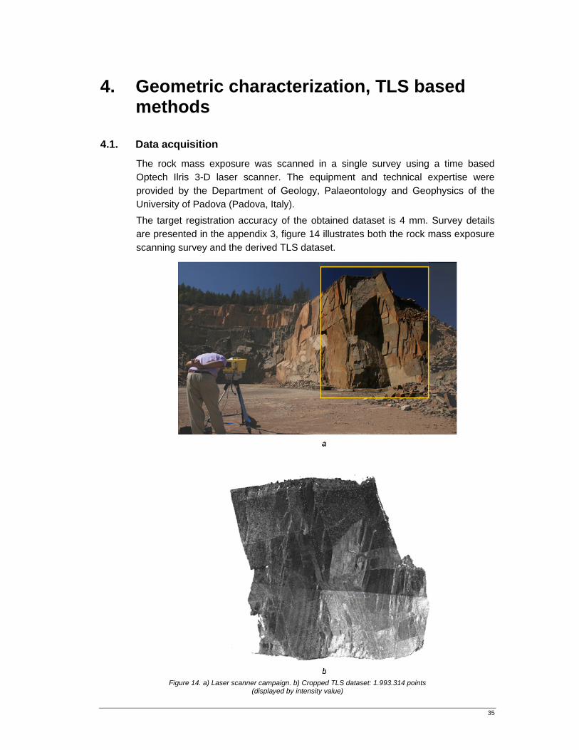
35
4. Geometric characterization, TLS based methods
4.1. Data acquisition
The rock mass exposure was scanned in a single survey using a time based Optech Ilris 3-D laser scanner. The equipment and technical expertise were provided by the Department of Geology, Palaeontology and Geophysics of the University of Padova (Padova, Italy). The target registration accuracy of the obtained dataset is 4 mm. Survey details are presented in the appendix 3, figure 14 illustrates both the rock mass exposure scanning survey and the derived TLS dataset.
Figure 14. a) Laser scanner campaign. b) Cropped TLS dataset: 1.993.314 points
(displayed by intensity value)
36
4.2. Dataset reorientation
Prior to realize the analysis, the TLS dataset was moved to its real orientation as measured in the field with the NS axis aligned with the y axis and the EW axis aligned with the x axis. Since there were not a precise georeference system in the study site, the reorientation of the dataset was achieved using two control surfaces on the rock face which their orientation was measured while performing the scan line mapping. This task was accomplished through a reorientation algorithm wrote by Van Knapen (2004), where the needed input are the measured (in field) orientations of the two control surfaces as well as their orientation in the scan. On these orientations, the algorithm calculates the orientation of one surface with the rotation matrix generated by the other. Rotation parameters and the deviation from the measured surface orientation with the orientation rotated with aid of the other are calculated. The parameters which introduce the smallest error are used to reorient all the dataset.
4.3. Data analysis to derive orientation information
Once the TLS dataset has been reoriented, it provides a detailed and accurate representation of rock mass exposure surface (see figure 15), but in order to derive geometric information parameters further analysis is required. As stated in section 2.4.2 two main approaches can be used to derive such information. In the present research, two of them have been used in order to compare its results. The first one is based on surface reconstruction and the second one on direct segmentation technique.
4.3.1. Surface reconstruction with 2D gridding and Delaunay triangulation
This method creates a regular 2D mesh on a virtual plane (parallel to the general trend of the scanned surface) and interpolates the distance between each node of such mesh and the scanned surface using the distances of its surrounding points through a linear interpolation algorithm. The resultant array of mesh nodes whit their z values is the structured forming a 3D surface using Delaunay triangulation. The nodes of such surface are then a spaced array of z values that overlay the original point cloud. The processing routine was accomplished using a trial version of the Split-FX® Software Ver.1.0 (Split Engineering LLC, 2007). Further details concerning this process are discussed by (Kemeny and Donovan, 2005).
4.3.1.1. Data edition
After reorienting the dataset (see section 4.2), and prior to perform the surface reconstruction it was necessary to remove all the data corresponding to those objects that not correspond to the rock surface to analyze (i.e. loose blocks on the ground and some erratic points that were present along the trajectory of the laser beam that were possibly originated by dust presence). This was important in order to avoid the generation of an erratic triangulated surface on the areas where such unrelated points appears.
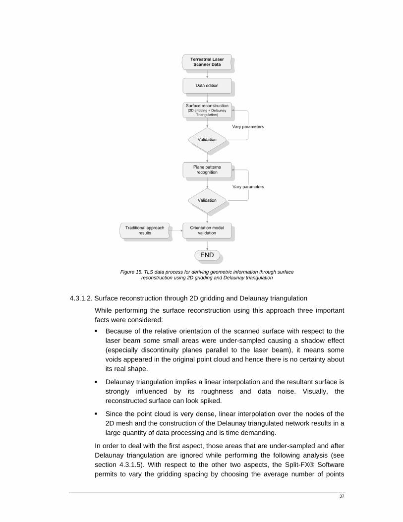
37
Figure 15. TLS data process for deriving geometric information through surface
reconstruction using 2D gridding and Delaunay triangulation
4.3.1.2. Surface reconstruction through 2D gridding and Delaunay triangulation
While performing the surface reconstruction using this approach three important facts were considered: Because of the relative orientation of the scanned surface with respect to the
laser beam some small areas were under-sampled causing a shadow effect (especially discontinuity planes parallel to the laser beam), it means some voids appeared in the original point cloud and hence there is no certainty about its real shape.
Delaunay triangulation implies a linear interpolation and the resultant surface is strongly influenced by its roughness and data noise. Visually, the reconstructed surface can look spiked.
Since the point cloud is very dense, linear interpolation over the nodes of the 2D mesh and the construction of the Delaunay triangulated network results in a large quantity of data processing and is time demanding.
In order to deal with the first aspect, those areas that are under-sampled and after Delaunay triangulation are ignored while performing the following analysis (see section 4.3.1.5). With respect to the other two aspects, the Split-FX® Software permits to vary the gridding spacing by choosing the average number of points
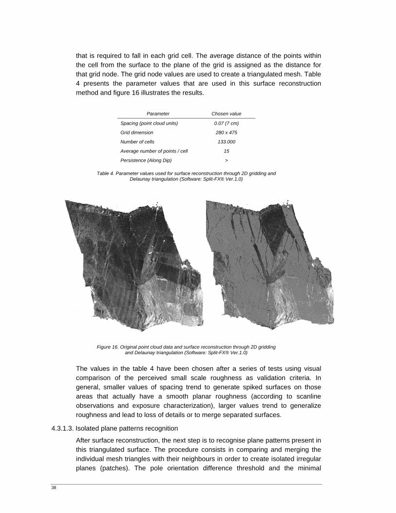
38
that is required to fall in each grid cell. The average distance of the points within the cell from the surface to the plane of the grid is assigned as the distance for that grid node. The grid node values are used to create a triangulated mesh. Table 4 presents the parameter values that are used in this surface reconstruction method and figure 16 illustrates the results.
Parameter Chosen value
Spacing (point cloud units) 0.07 (7 cm)
Grid dimension 280 x 475
Number of cells 133.000
Average number of points / cell 15
Persistence (Along Dip) >
Table 4. Parameter values used for surface reconstruction through 2D gridding and Delaunay triangulation (Software: Split-FX® Ver.1.0)
Figure 16. Original point cloud data and surface reconstruction through 2D gridding and Delaunay triangulation (Software: Split-FX® Ver.1.0)
The values in the table 4 have been chosen after a series of tests using visual comparison of the perceived small scale roughness as validation criteria. In general, smaller values of spacing trend to generate spiked surfaces on those areas that actually have a smooth planar roughness (according to scanline observations and exposure characterization), larger values trend to generalize roughness and lead to loss of details or to merge separated surfaces.
4.3.1.3. Isolated plane patterns recognition
After surface reconstruction, the next step is to recognise plane patterns present in this triangulated surface. The procedure consists in comparing and merging the individual mesh triangles with their neighbours in order to create isolated irregular planes (patches). The pole orientation difference threshold and the minimal
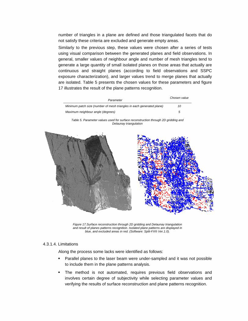
4.3.1.4
number onot satisfySimilarly using visugeneral, sgenerate continuouexposure are isolate17 illustra
Minimum
Maximu
Tab
Figan
4. Limitation
Along the Paralle
to incl
The minvolveverifyi
of triangles iy these criteto the previual comparissmaller valua large qua
us and stracharacteriz
ed. Table 5 ates the resu
m patch size (num
um neighbour ang
ble 5. Parameter
gure 17.Surface nd result of plane
blue, and
s
process soel planes to ude them in
method is es certain dng the resul
n a plane aria are excluious step, thson betweenes of neighbntity of sma
aight planesation), and presents th
ult of the plan
Paramet
mber of mesh tri
gle (degrees)
values used for Delau
reconstruction thes patterns recog
excluded areas
me lacks wethe laser be
the plane p
not automadegree of suts of surface
are defined auded and gehese valuesn the generabour angle all isolated pls (accordinglarger valuee chosen vane patterns r
ter
iangles in each g
surface reconstr
unay triangulation
hrough 2D griddignition. Isolated p
in red. (Software
ere identifiedeam were u
patterns anal
ated, requirubjectivity we reconstruc
and those tenerate empts were chosated planes and number lanes on thog to field
es trend to malues for therecognition.
generated plane)
ruction through 2n
ing and Delaunayplane patterns are: Split-FX® Ver.
d as follows:nder-samplelysis.
es previouswhile selectition and pla
riangulated ty areas.
sen after a sand field obof mesh tria
ose areas thobservation
merge planeese paramet
Chosen val
10
5
2D gridding and
y triangulation re displayed in .1.0).
ed and it wa
s field obseng parametne patterns
facets that
series of tesbservations. angles tend at actually as and SSP
es that actuaters and figu
lue
as not possib
ervations aer values arecognition.
do
sts In to
are PC ally ure
ble
and and
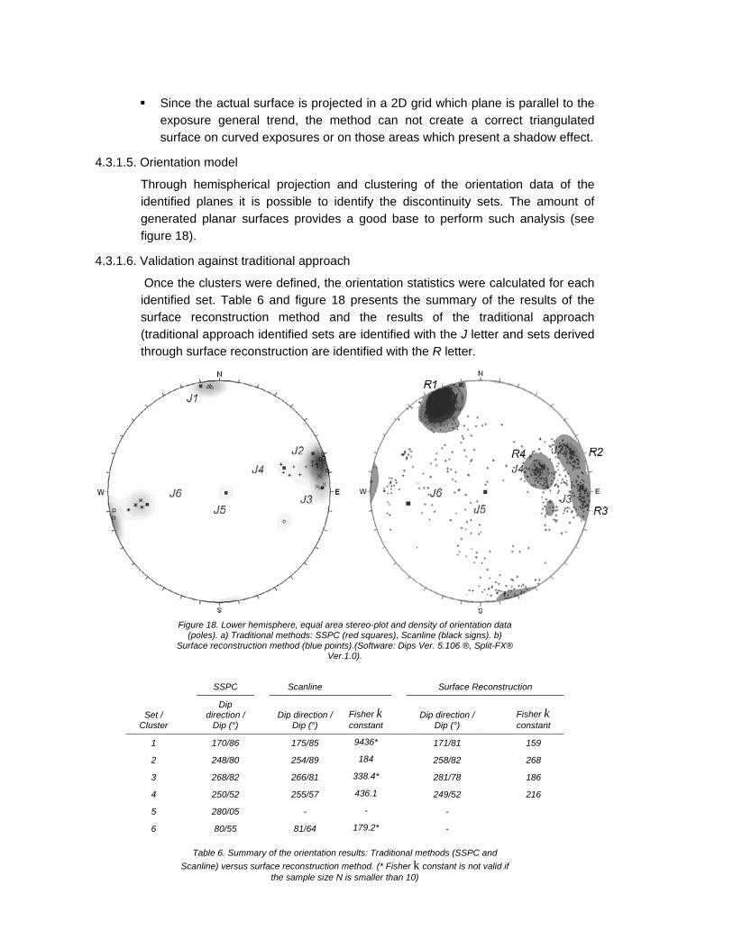
4
4
4.3.1.5. Orie
Throidengenfigu
4.3.1.6. Vali
Onidensurf(tradthro
Set /Clust
1
2
3
4
5
6
Since the acexposure gsurface on c
entation mod
ough hemisntified planenerated planre 18).
dation again
ce the clustntified set. Tface reconsditional appr
ough surface
Figure 18. L(poles). a
Surface reco
SS
/ ter
Ddirec
Dip
170
248
268
250
280
80/
Table 6.Scanline) v
ctual surfaceeneral trend
curved expo
del
spherical proes it is possar surfaces
nst traditiona
ers were deTable 6 andstruction mroach identife reconstruct
Lower hemisphera) Traditional metonstruction meth
SPC S
Dip ction / p (°)
Dip
0/86
8/80
8/82
0/52
0/05
/55
Summary of theversus surface re
the s
e is projected, the methsures or on
ojection andsible to iden
provides a
al approach
efined, the or figure 18 pethod and fied sets aretion are iden
re, equal area stethods: SSPC (re
hod (blue points).Ver.1.0
Scanline
p direction / Dip (°)
Fc
175/85
254/89
266/81 3
255/57
-
81/64
e orientation resueconstruction mesample size N is
ed in a 2D ghod can nothose areas
d clustering ntify the dis good base
rientation stapresents the
the resultse identified wntified with th
ereo-plot and ded squares), Scan(Software: Dips
0).
Fisher k onstant
9436*
184
338.4*
436.1
-
179.2*
ults: Traditional method. (* Fisher k
smaller than 10)
rid which plaot create a s which pres
of the oriescontinuity se to perform
atistics weree summary os of the twith the J lethe R letter.
nsity of orientationline (black signsVer. 5.106 ®, Sp
Surface Re
Dip direction / Dip (°)
171/81
258/82
281/78
249/52
-
-
methods (SSPC ak constant is not )
ane is paralcorrect triaent a shado
entation datsets. The am such analy
e calculated of the resultraditional atter and sets
on data s). b) plit-FX®
econstruction
Fisher kconstan
159
268
186
216
and valid if
lel to the ngulated w effect.
a of the mount of ysis (see
for each ts of the
approach s derived
k nt

41
In view of the results (see table 6 and figure 18) next observations can be made:
The sub-vertical discontinuity sets J1, J2, J3 and J4 (and correspondent R1, R2, R3 and R4) were identified by both approaches and their results are comparable. According to the density plot, the discontinuity set was the most sampled, while the sub-vertical set J6 and sub-horizontal J5 were not identified by the present method.
The reason for this is that sets J1, J2, J3 and J4 are well exposed on the surface of the current cuts. On the other hand, the orientation sets J5 and J6 presents two problems a) their discontinuity planes are perpendicular to the trend of the surface where they are exposed, hence just its trace appears on such surface and b) they were under-sampled due their relative orientation respect to the laser beam.
When comparing with the traditional approach (scanline), the larger quantity of orientation data permit to verify the presence of discontinuity sets J2, J3 and J4 that were identified by SSPC system. Also is possible have a better impression of the orientation variability of each of these clusters.
Although that there is correspondence between the identified sets, there is a difference in orientation values. This may be due to the method which was used to reorient the point cloud (see section 4.2) and to human bias and instrument error while measuring orientations on the field.
Even though there is additional data, is not possible to verify if the poles around 280/55 correspond to outliers or are part of an under-sampled discontinuity set.
4.3.2. Direct segmentation with 3D Hough transformation and least squares
As discussed in section 2.4.2.2 through direct segmentation process, flat planes are recognised within the point cloud, and the point cloud data is classified into subsets of points that belong to a particular plane. The segmented point cloud is then processed to derive the individual plane equations and determine their geometrical properties. The process was mainly accomplished according to the methodology proposed by(Bezdek, 1981; Slob et al., 2006; Slob and van Knapen, 2006) which includes the following steps (see figure 19): Creation of a spatial structure within the point cloud data and plane patterns
recognition through Hough transformation and least squares estimation. This task was implemented in PCM2 (Point Cloud Mapper) software (Vosselman et al., 2005).
Planes parameterization and computation of planes orientation. This was implemented through Matlab ® codes by Slob (2006).
Discontinuity set identification through the fuzzy k-means clustering algorithm using Matlab ® code by van Knapen (2006).
Set orientation statistics computation using Matlab ® code by Slob (2006)

42
Figure 19. TLS data process for deriving geometric information direct segmentation and least squares estimation
4.3.2.1. Creation of a spatial structure
The creation of a spatial structure within the point cloud permits to establish an internal network that accelerates the searching process while performing the segmentation. Kd-tree structure (Bentley, 1975) is a commonly used alternative to create such a searching structure (see section 2.6). PCM2 include an algorithm to build this Kd-tree structure, the parameters where used are shown in the table 7.
Parameter Chosen value
Storage model Kd-tree
Distance metric 3D
Number of neighbours in kd-tree* 20
Table 7. Kd-tree structure parameters (* Refers to the average number of points that each kd-tree cell contain)
43
4.3.2.2. Point cloud segmentation through Hough transformation and least squares
The use of Hough transformation to recognize linear patterns in 2D images can be extended to a 3D space to recognize plane patterns in a point cloud data. This idea is also implemented in the PCM2 software (Vosselman et al., 2005). Once its spatial structure has been constructed, the point cloud is systematically analyzed in order to determine if neighbouring points belongs to the same plane. Hough transformation permits to identify an initial seed point that potentially belongs to a plane, after this, a determined number of its nearest neighbours are tested using a least square estimation algorithm to verify if they belong to the same plane. If this is the case, all these points are labelled with a code that identifies also the plane they belong to, otherwise new seed points are found and the process is repeated up to all the points are labelled. The executed process in PCM2 is accomplished in a number of stages where various parameters are used to define searching and distance thresholds as follows: Definition of the connected component parameters: Here two parameters have
to be defined: a) maximum distance between points (which defines a neighbourhood area around a given point) and b) minimum number of points (which defines a number of neighbours around a given point). If these conditions are not satisfied by two given points, then they are considered as not connected.
Seed selection parameters: This specifies how the seed points are going to be chosen from among all the potential points present in the Hough space. The parameters are: a) Seed neighbourhood definition (either a number of direct neighbours or a search radius around the selected random point must be specified), b) Maximum slope angle (permits to ignore seed points which are present in stepped planes), c) Bin size slope angle (indicates the size in which the angle parameters in Hough space is discretized and hence the threshold which defines if seed points are or not coplanar), d) Bin size distance (indicates the size in which distance parameters in Hough space is discretized and hence the threshold with defines if seed points about the surface of the current plane should be classified as belonging to that plane), e) Minimum number of seed points (permits to abandon the process if few seed points are found to belong to a specific plane), f) Maximum distance to the plane (defines an orthogonal distance to the current plane, all points below this distance can be used as new seed points).
Surface growing parameters: This specifies how the plane is going to grow around the found seed points. The parameters are: a) Surface model (either a planar or smooth model can be used), b) Surface growing neighbourhood definition (either a number of direct neighbours or a search radius around the seed points must be specified), c) Surface growing radius (defines the search radius around the seed points), d) Maximum distance to surface (all points below this distance are assigned to the current plane), e) Competing surfaces (this optional parameter permits to determine if previously labelled points match in a better way with the current growing plane).
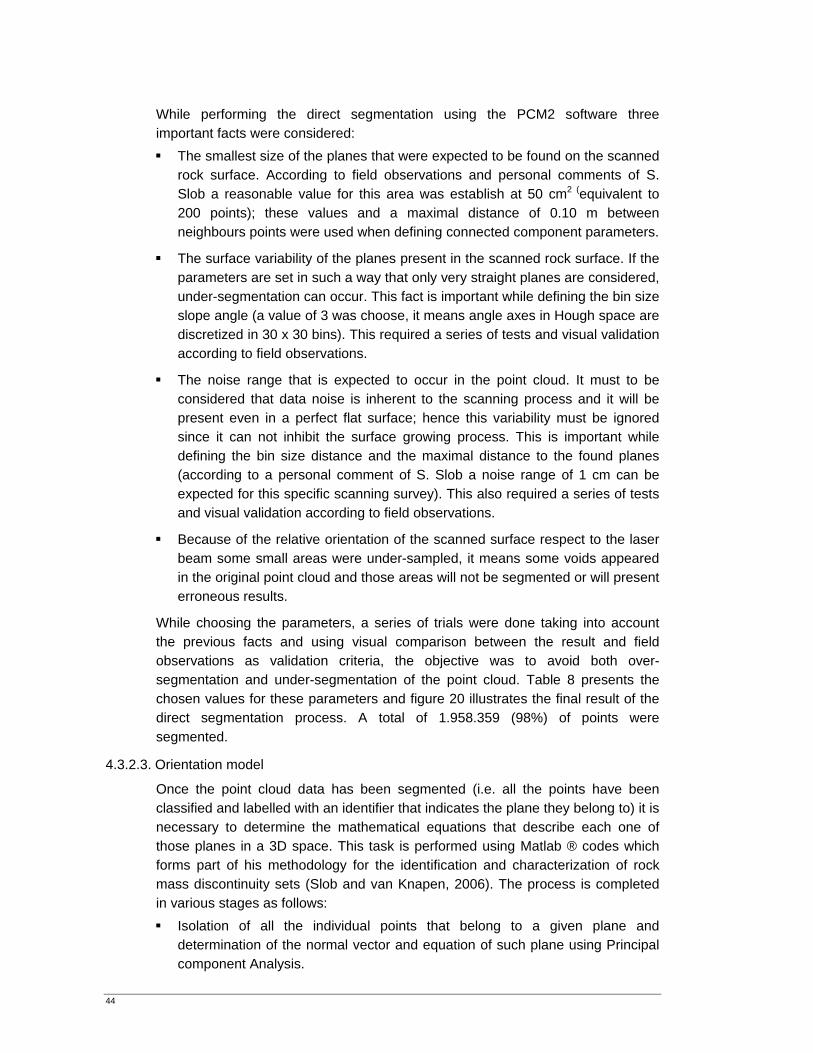
44
While performing the direct segmentation using the PCM2 software three important facts were considered: The smallest size of the planes that were expected to be found on the scanned
rock surface. According to field observations and personal comments of S. Slob a reasonable value for this area was establish at 50 cm2 (equivalent to 200 points); these values and a maximal distance of 0.10 m between neighbours points were used when defining connected component parameters.
The surface variability of the planes present in the scanned rock surface. If the parameters are set in such a way that only very straight planes are considered, under-segmentation can occur. This fact is important while defining the bin size slope angle (a value of 3 was choose, it means angle axes in Hough space are discretized in 30 x 30 bins). This required a series of tests and visual validation according to field observations.
The noise range that is expected to occur in the point cloud. It must to be considered that data noise is inherent to the scanning process and it will be present even in a perfect flat surface; hence this variability must be ignored since it can not inhibit the surface growing process. This is important while defining the bin size distance and the maximal distance to the found planes (according to a personal comment of S. Slob a noise range of 1 cm can be expected for this specific scanning survey). This also required a series of tests and visual validation according to field observations.
Because of the relative orientation of the scanned surface respect to the laser beam some small areas were under-sampled, it means some voids appeared in the original point cloud and those areas will not be segmented or will present erroneous results.
While choosing the parameters, a series of trials were done taking into account the previous facts and using visual comparison between the result and field observations as validation criteria, the objective was to avoid both over-segmentation and under-segmentation of the point cloud. Table 8 presents the chosen values for these parameters and figure 20 illustrates the final result of the direct segmentation process. A total of 1.958.359 (98%) of points were segmented.
4.3.2.3. Orientation model
Once the point cloud data has been segmented (i.e. all the points have been classified and labelled with an identifier that indicates the plane they belong to) it is necessary to determine the mathematical equations that describe each one of those planes in a 3D space. This task is performed using Matlab ® codes which forms part of his methodology for the identification and characterization of rock mass discontinuity sets (Slob and van Knapen, 2006). The process is completed in various stages as follows: Isolation of all the individual points that belong to a given plane and
determination of the normal vector and equation of such plane using Principal component Analysis.
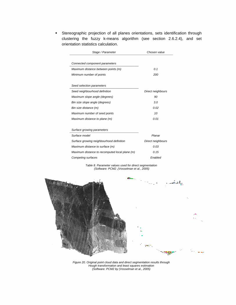
Stereoclusteorienta
C
M
M
S
S
M
B
B
M
M
S
S
S
M
M
C
ographic proring the fuation statistic
S
Connected comp
Maximum distanc
Minimum number
Seed selection p
Seed neighbourh
Maximum slope a
Bin size slope an
Bin size distance
Maximum numbe
Maximum distanc
Surface growing
Surface model
Surface growing
Maximum distanc
Maximum distanc
Competing surfac
Table
Figure 20. OriginHou
(
ojection of auzzy k-meacs calculatio
Stage / Paramete
ponent paramete
ce between poin
r of points
arameters
hood definition
angle (degrees)
ngle (degrees)
e (m)
er of seed points
ce to plane (m)
parameters
neighbourhood d
ce to surface (m)
ce to recomputed
ces
8. Parameter va (Software: PCM
nal point cloud dugh transformatio(Software: PCM2
all planes orans algorithon.
er
rs
ts (m)
definition
)
d local plane (m)
alues used for dirM2 ,(Vosselman e
data and direct seon and least squa2 by (Vosselman
rientations, shm (see se
Chosen
0
20
Direct ne
9
3
0.
1
0.
Pla
Direct ne
0.
) 0.
Ena
rect segmentatioet al., 2005)
egmentation resuares estimationet al., 2005)
sets identificection 2.6.2
n value
.1
00
eighbours
90
.0
02
10
01
anar
eighbours
03
15
abled
n
ults through
cation throu2.4), and s
gh set
4
Althappthe algoindediscsubprevfourapppres
4.3.2.4. Vali
Tabsegappcurr
In view of thmade:
hough fuzzyproach to de
number of orithm basedexes did notcontinuity seb-horizontalsvious experir. Below thi
pear; insteadsented in the
dation again
ble 9 and mentation m
proach deriverent method
Figure 21. (poles). a
Di
he results pre
The sub-veD2, D3 andcomparablemethod (thismost samplewere not ide
y k-means climit discontexpected se
d on validity match with
ets was spec sets were iiences the ns value, isod already de figure 21.
nst traditiona
figure 21 pmethod anded sets are are identifie
Low hemispherea) Traditional metirect segmentatio
esented in th
rtical discond D4) were. However s is discusseed (322 planentified by th
clustering ainuity sets oets must to
y indexes (sethe expecte
cified accorddentified usnumber of tolated clustedefined sets
al approach
presents thd the resulidentified w
ed with the D
e, equal area stethods: SSPC (reon (black signs).
he table 9 an
ntinuity sets e identified
the angulared in sectionnes), while the present m
algorithm is on the base o
be definedee section 2
ed results; thding to previing the preshe remaininers are mers are cluste
e summaryts of the tith the J lett
D letter.
reo-plot and dend squares), Scan(Software: Dips
nd figure 21
J1, J2, J3 aby both apr differencesn 4.3.2.5). The sub-verti
method.
supposed of their orien prior to ex2.6.2.4). In therefore the ous observa
sent method,ng (sub-vertirged and abered again.
y of the retraditional ater and sets
nsity of orientationline (black signsVer. 5.106 ®)
next observ
and J4 (andproaches as are large
The discontincal set J6 a
to be an ontation homoxecute the cthis case thenumber of e
ations. In ge, so accordincal) sets wa
bove it no nThe final
esults of thapproach (tr
derived thro
n data s). b)
vations can b
d correspondnd their resr than the nuity set D1 nd sub-horiz
objective ogeneity, clustering e validity expected eneral no ng to the as set at new sets result is
he direct raditional ough the
be
dent D1, sults are previous was the
zontal J5
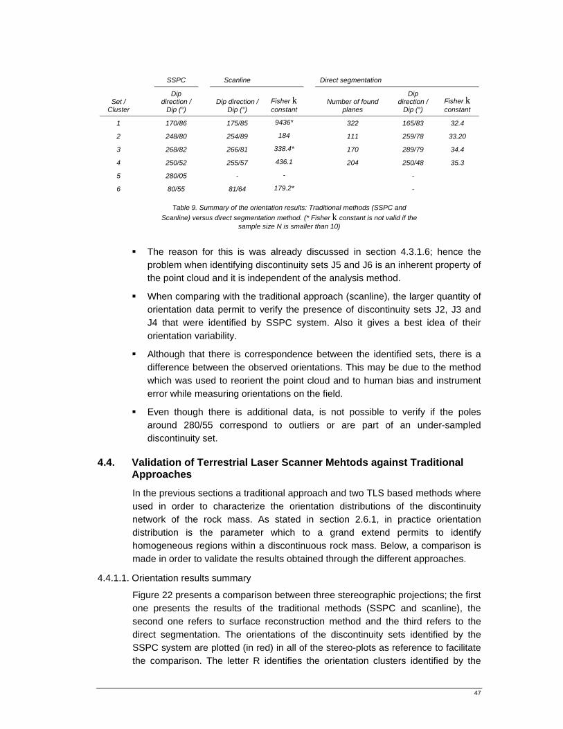
47
SSPC Scanline Direct segmentation
Set / Cluster
Dip direction /
Dip (°) Dip direction /
Dip (°) Fisher k constant
Number of found planes
Dip direction /
Dip (°) Fisher k constant
1 170/86 175/85 9436* 322 165/83 32.4
2 248/80 254/89 184 111 259/78 33.20
3 268/82 266/81 338.4* 170 289/79 34.4
4 250/52 255/57 436.1 204 250/48 35.3
5 280/05 - - -
6 80/55 81/64 179.2* -
Table 9. Summary of the orientation results: Traditional methods (SSPC and Scanline) versus direct segmentation method. (* Fisher k constant is not valid if the
sample size N is smaller than 10)
The reason for this is was already discussed in section 4.3.1.6; hence the problem when identifying discontinuity sets J5 and J6 is an inherent property of the point cloud and it is independent of the analysis method.
When comparing with the traditional approach (scanline), the larger quantity of orientation data permit to verify the presence of discontinuity sets J2, J3 and J4 that were identified by SSPC system. Also it gives a best idea of their orientation variability.
Although that there is correspondence between the identified sets, there is a difference between the observed orientations. This may be due to the method which was used to reorient the point cloud and to human bias and instrument error while measuring orientations on the field.
Even though there is additional data, is not possible to verify if the poles around 280/55 correspond to outliers or are part of an under-sampled discontinuity set.
4.4. Validation of Terrestrial Laser Scanner Mehtods against Traditional Approaches
In the previous sections a traditional approach and two TLS based methods where used in order to characterize the orientation distributions of the discontinuity network of the rock mass. As stated in section 2.6.1, in practice orientation distribution is the parameter which to a grand extend permits to identify homogeneous regions within a discontinuous rock mass. Below, a comparison is made in order to validate the results obtained through the different approaches.
4.4.1.1. Orientation results summary
Figure 22 presents a comparison between three stereographic projections; the first one presents the results of the traditional methods (SSPC and scanline), the second one refers to surface reconstruction method and the third refers to the direct segmentation. The orientations of the discontinuity sets identified by the SSPC system are plotted (in red) in all of the stereo-plots as reference to facilitate the comparison. The letter R identifies the orientation clusters identified by the
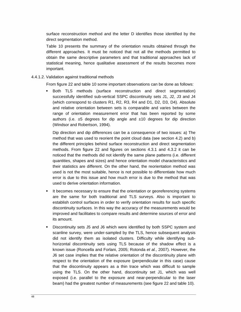
48
surface reconstruction method and the letter D identifies those identified by the direct segmentation method. Table 10 presents the summary of the orientation results obtained through the different approaches. It must be noticed that not all the methods permitted to obtain the same descriptive parameters and that traditional approaches lack of statistical meaning, hence qualitative assessment of the results becomes more important.
4.4.1.2. Validation against traditional methods
From figure 22 and table 10 some important observations can be done as follows: Both TLS methods (surface reconstruction and direct segmentation)
successfully identified sub-vertical SSPC discontinuity sets J1, J2, J3 and J4 (which correspond to clusters R1, R2, R3, R4 and D1, D2, D3, D4). Absolute and relative orientation between sets is comparable and varies between the range of orientation measurement error that has been reported by some authors (i.e. ±5 degrees for dip angle and ±10 degrees for dip direction (Windsor and Robertson, 1994).
Dip direction and dip differences can be a consequence of two issues: a) The method that was used to reorient the point cloud data (see section 4.2) and b) the different principles behind surface reconstruction and direct segmentation methods. From figure 22 and figures on sections 4.3.1 and 4.3.2 it can be noticed that the methods did not identify the same plane patterns (i.e. different quantities, shapes and sizes) and hence orientation model characteristics and their statistics are different. On the other hand, the reorientation method was used is not the most suitable, hence is not possible to differentiate how much error is due to this issue and how much error is due to the method that was used to derive orientation information.
It becomes necessary to ensure that the orientation or georeferencing systems are the same for both traditional and TLS surveys. Also is important to establish control surfaces in order to verify orientation results for such specific discontinuity surfaces. In this way the accuracy of the measurements would be improved and facilitates to compare results and determine sources of error and its amount.
Discontinuity sets J5 and J6 which were identified by both SSPC system and scanline survey, were under-sampled by the TLS, hence subsequent analysis did not identify them as isolated clusters. Difficulty while identifying sub-horizontal discontinuity sets using TLS because of the shadow effect is a known issue (Roncella and Forlani, 2005; Rotonda et al., 2007). However, the J6 set case implies that the relative orientation of the discontinuity plane with respect to the orientation of the exposure (perpendicular in this case) cause that the discontinuity appears as a thin trace which was difficult to sample using the TLS. On the other hand, discontinuity set J1, which was well exposed (i.e. parallel to the exposure and near-perpendicular to the laser beam) had the greatest number of measurements (see figure 22 and table 10).
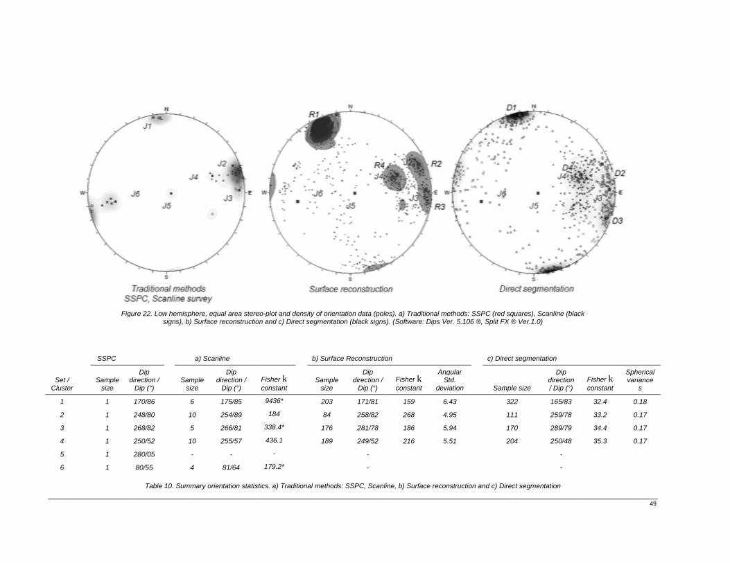
SetClus
1
2
3
4
5
6
Fig
SSPC
t / ster
Sample size
1
1
1
1
1
1
gure 22. Low hemisphsigns), b)
Dip direction /
Dip (°) Sam
siz
170/86 6
248/80 1
268/82 5
250/52 1
280/05 -
80/55 4
Table 10. Summ
here, equal area stereSurface reconstructio
a) Scanline
mple ze
Dip direction /
Dip (°)
6 175/85
0 254/89
5 266/81
0 255/57
- -
4 81/64
mary orientation statis
eo-plot and density ofon and c) Direct segm
b) S
Fisher k constant
Sa
9436*
184
338.4*
436.1
-
179.2*
stics. a) Traditional me
f orientation data (polmentation (black signs
Surface Reconstructio
ample size
Dip direction /
Dip (°)
203 171/81
84 258/82
176 281/78
189 249/52
-
-
ethods: SSPC, Scanl
les). a) Traditional mes). (Software: Dips Ve
on
Fisher k constant
AngSt
devia
159 6.4
268 4.
186 5.
216 5.
line, b) Surface recon
ethods: SSPC (red sqer. 5.106 ®, Split FX ®
c) Direct
gular td. ation Sample
43 32
95 11
94 17
51 20
nstruction and c) Direc
quares), Scanline (bla® Ver.1.0)
t segmentation
e size
Dip direction / Dip (°)
22 165/83
11 259/78
70 289/79
04 250/48
-
-
ct segmentation
ck
Fisher k constant
Sphevaria
s
32.4 0.1
33.2 0.1
34.4 0.1
35.3 0.1
49
rical ance s
18
17
17
17

51
Scanline identified a single isolated discontinuity at 280/55. TLS results present some degree of clustering around this value (see figure 22), hence it is possible that a seventh discontinuity set is present in the rock mass. Although fuzzy k-means clustering algorithm did not identify more clusters in this region, further analysis would be required in order to establish if it is a non well exposed set (hence under-sampled) or if sets 2, 3 or 4 have such an orientation variability.
Even SSPC system permitted to avoid scanline biases (i.e. because of its orientation and limited length) its information should be considered as “representative” since it is not possible to verify its accuracy. In theory scanline can complement such information and provide statistical support in order to validate SSPC measurements and analyse sets variability, however in the present case, the scanline data did not provide such statistical support due to the small number of measurements that were done.
On the other hand, TLS methods gave a better impression of the isolation, mean orientation and variability of each one of the identified sets. Orientation distribution (and hence variability analysis) is an important issue when modelling a discontinuity network (see section 2.6.2). Further analysis is required in order to establish the suitability of TLS derived orientation data when modelling orientation distribution.
Semi-automated approach (it means to manually digitize discontinuity planes over the point cloud according to the engineering criteria) becomes an alternative when analysing TLS data. However it is time consuming and would also involve human bias, for these reasons was not used along this research.
As a final remark, attending the results presented in the table 10 and taking SSPC results as reference a set by set comparison is presented as follows: SSPC discontinuity set J1: This sub-vertical set was unequivocally identified as a
single and isolated discontinuity set by all the methods (traditional and TLS), nonetheless the value of its mean orientation (dip direction / dip) varies in each method. It was the most sampled by the TLS.
SSPC discontinuity set J2: This sub-vertical set was identified by all the methods (traditional and TLS), just as set J1, the J2 derived mean orientation (dip direction / dip) is different in each method.
SSPC discontinuity set J3: This sub-vertical set was identified by all the methods (traditional and TLS). Its derived mean orientation (dip direction / dip) is also different in each method.
SSPC discontinuity set J4: This oblique set was identified by all the methods (traditional and TLS). Its derived mean orientation (dip direction / dip) is also different in each method.
SSPC discontinuity set J5: This sub-horizontal set was not identified by the TLS methods. Its relative orientation respect to the laser beam produced a shadow effect and hence it was under-sampled.
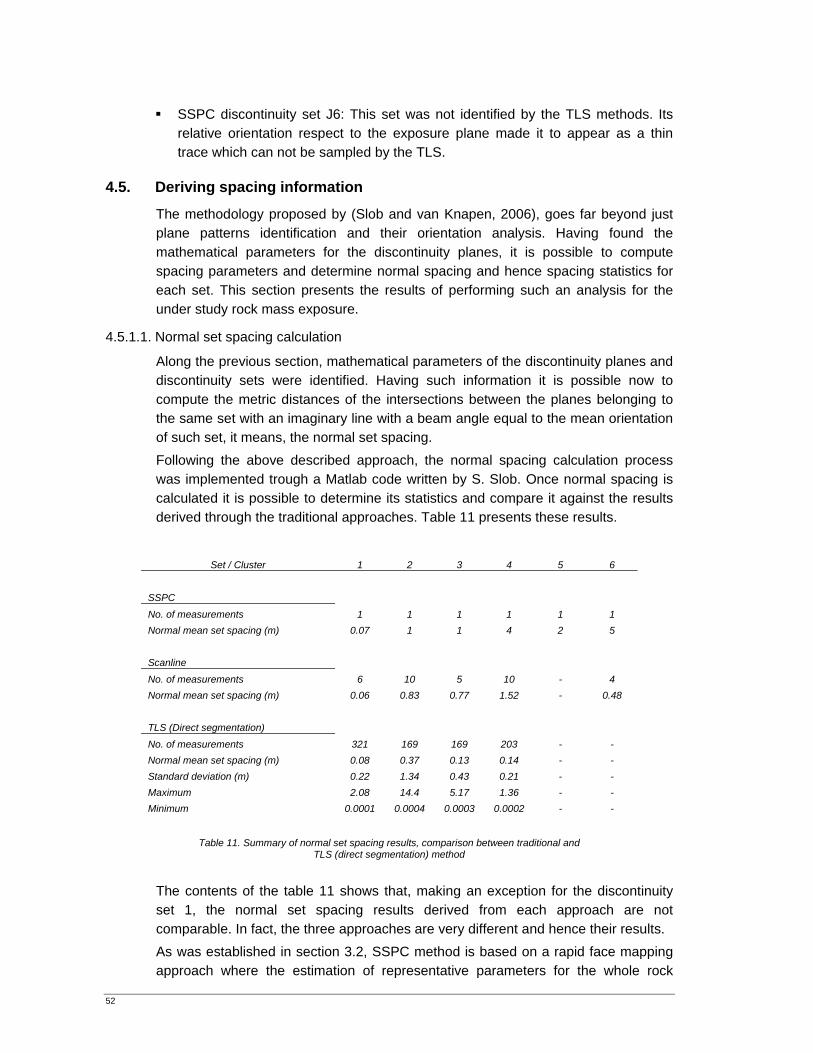
52
SSPC discontinuity set J6: This set was not identified by the TLS methods. Its relative orientation respect to the exposure plane made it to appear as a thin trace which can not be sampled by the TLS.
4.5. Deriving spacing information
The methodology proposed by (Slob and van Knapen, 2006), goes far beyond just plane patterns identification and their orientation analysis. Having found the mathematical parameters for the discontinuity planes, it is possible to compute spacing parameters and determine normal spacing and hence spacing statistics for each set. This section presents the results of performing such an analysis for the under study rock mass exposure.
4.5.1.1. Normal set spacing calculation
Along the previous section, mathematical parameters of the discontinuity planes and discontinuity sets were identified. Having such information it is possible now to compute the metric distances of the intersections between the planes belonging to the same set with an imaginary line with a beam angle equal to the mean orientation of such set, it means, the normal set spacing. Following the above described approach, the normal spacing calculation process was implemented trough a Matlab code written by S. Slob. Once normal spacing is calculated it is possible to determine its statistics and compare it against the results derived through the traditional approaches. Table 11 presents these results.
Set / Cluster 1 2 3 4 5 6
SSPC
No. of measurements 1 1 1 1 1 1 Normal mean set spacing (m) 0.07 1 1 4 2 5 Scanline No. of measurements 6 10 5 10 - 4 Normal mean set spacing (m) 0.06 0.83 0.77 1.52 - 0.48 TLS (Direct segmentation)
No. of measurements 321 169 169 203 - - Normal mean set spacing (m) 0.08 0.37 0.13 0.14 - - Standard deviation (m) 0.22 1.34 0.43 0.21 - - Maximum 2.08 14.4 5.17 1.36 - - Minimum 0.0001 0.0004 0.0003 0.0002 - -
Table 11. Summary of normal set spacing results, comparison between traditional and
TLS (direct segmentation) method The contents of the table 11 shows that, making an exception for the discontinuity set 1, the normal set spacing results derived from each approach are not comparable. In fact, the three approaches are very different and hence their results. As was established in section 3.2, SSPC method is based on a rapid face mapping approach where the estimation of representative parameters for the whole rock
53
mass exposure was performed according to engineering criteria and experience. On the other hand, scanline survey concentrates in acquiring discontinuity information over a 2D surface along a single direction with a limited length. These two methods differ a lot from the TLS method, where in fact an imaginary scanline beams into a larger 3D model of the discontinuity set which present orientation variability and can generate erratic intersections with such planes along its trajectory. On the other hand, because of local variations, a single discontinuity surface can be over segmented and generate several small planes. The normal set spacing between this large quantities of close planes is very small and hence the normal set spacing is underestimated by this method. Further analysis is required in order to find the way to determine the normal set spacing in such a model or to establish the relation between the set spacing distribution derived from traditional methods and the spacing distribution derived from such a 3D model.
5. Detecting and mapping internal discontinuity network, Ground Penetrating Radar based method
Ground Penetrating Radar (GPR) has been used for discontinuity detection and mapping in 2D in volcanic, metamorphic and sedimentary rocks such as granite, gneiss and limestone (Toshioka et al., 1995); (Stevens et al., 1995; Porsani et al., 2006) and the comparison between structural observations on surface (Grandjean and Gourry, 1996), borehole measurements and post mining observations (Deparis et al., 2007) have shown the potential of GPR for discontinuity characterization (section 2.5).This section presents the principles and methodology that was followed in order to detect and characterize the internal discontinuity network of the rock mass exposures.
5.1. Methodology
Four steps were executed to evaluate GPR as methodology to detect and map internal discontinuities within the rock mass, a) establishing the viability of the GPR method and GPR survey requirements taking into account the research objective, the rock mass characteristics, and its discontinuity network, b) data acquisition, c) processing the GPR data in order to detect the features of interest and d) interpretation, presentation and validation of the results (figure 23 shows the proposed methodology).
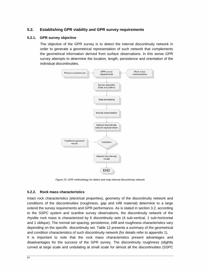
54
5.2. Establishing GPR viability and GPR survey requirements
5.2.1. GPR survey objective
The objective of the GPR survey is to detect the internal discontinuity network in order to generate a geometrical representation of such network that complements the geometrical information derived from surface observations. In this sense GPR survey attempts to determine the location, length, persistence and orientation of the individual discontinuities.
Figure 23. GPR methodology for detect and map internal discontinuity network
5.2.2. Rock mass characteristics
Intact rock characteristics (electrical properties), geometry of the discontinuity network and conditions of the discontinuities (roughness, gap and infill material) determine to a large extend the survey requirements and GPR performance. As is stated in section 3.2, according to the SSPC system and scanline survey observations, the discontinuity network of the rhyolite rock mass is characterized by 6 discontinuity sets (4 sub-vertical, 1 sub-horizontal and 1 oblique). The normal set spacing, persistence, infill and roughness characteristics vary depending on the specific discontinuity set. Table 12 presents a summary of the geometrical and condition characteristics of such discontinuity network (for details refer to appendix 1). It is important to note that the rock mass characteristics present advantages and disadvantages for the success of the GPR survey. The discontinuity roughness (slightly curved at large scale and undulating at small scale for almost all the discontinuities (SSPC
55
characterization, Hack et al., 2003) facilitates normal incidence of the GPR signal, Normal incidence increases change that a decent signal is reflected. The difference between electrical properties of intact rock and infill material is favorable for GPR signal reflection. On the other hand, small openness of discontinuities with many contact points between discontinuity walls and the relative complexity of the discontinuity network may negatively affect GPR performance, and may make the interpretation of the results more difficult. This issue is further dealt with and discussed in section 5.1.1.3.
Set
Dip direction /
Dip (°)
Normal set
spacing (m)
Persist. Along strike (m)
Persist. Along dip (m)
Rough. Large scale
Rough. Small scale
Infill material
Gap (cm)
1 170/86 0.07 > > straight smooth planar
soft sheared fine
(washed clay)
< 1 cm
2 248/80 1 > > curved smooth undulating
non softening &
sheared (fine)
< 1 cm
3 268/82 1 0.07 3 curved smooth undulating no infill < 1 cm
4 250/52 4 0.5 0.5 - smooth undulating no infill < 1 cm
5 280/05 2 > > straight smooth undulating
non softening &
sheared (fine)
< 1 cm
6 80/55 5 > > wavy rough stepped
non softening &
sheared (fine)
< 1 cm
Table 12. Summary of the geometrical and condition characteristics of the
discontinuity network. SSPC system, (Hack, 1998, Hack et. al, 2003)
5.2.3. GPR performance for detecting discontinuities
As was stated in section 2.5.2, GPR has been used to detect and map internal discontinuities in volcanic, metamorphic and sedimentary rocks (Toshioka et al., 1995); (Stevens et al., 1995; Porsani et al., 2006). Experience has shown that the feasibility of GPR technique is conditioned by (Grandjean and Gourry, 1996): a) The difference of dielectric impedance between intact rock and infill material
within the discontinuities. If such difference is large enough, reflection of the transmitted energy by the GPR can be recorded (Parasnis, 1997).
b) The penetration versus resolution. The higher the GPR signal frequency the better the resolution is, but on the other hand the higher the frequency, the higher the attenuation is.
c) The complexity of the discontinuity network. Discontinuities must be sufficiently opened and separated from each other; otherwise they can create a complex reflectivity pattern and increase attenuation. Multiple-reflections and 3D
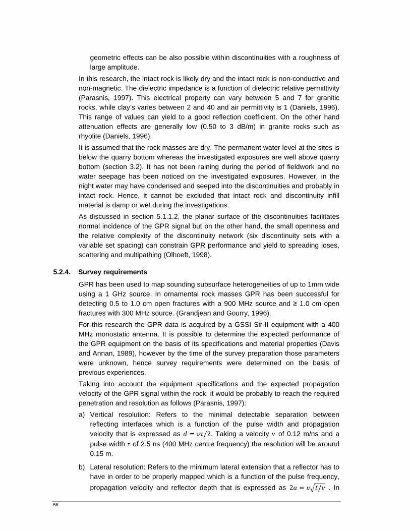
56
geometric effects can be also possible within discontinuities with a roughness of large amplitude.
In this research, the intact rock is likely dry and the intact rock is non-conductive and non-magnetic. The dielectric impedance is a function of dielectric relative permittivity (Parasnis, 1997). This electrical property can vary between 5 and 7 for granitic rocks, while clay’s varies between 2 and 40 and air permittivity is 1 (Daniels, 1996). This range of values can yield to a good reflection coefficient. On the other hand attenuation effects are generally low (0.50 to 3 dB/m) in granite rocks such as rhyolite (Daniels, 1996). It is assumed that the rock masses are dry. The permanent water level at the sites is below the quarry bottom whereas the investigated exposures are well above quarry bottom (section 3.2). It has not been raining during the period of fieldwork and no water seepage has been noticed on the investigated exposures. However, in the night water may have condensed and seeped into the discontinuities and probably in intact rock. Hence, it cannot be excluded that intact rock and discontinuity infill material is damp or wet during the investigations. As discussed in section 5.1.1.2, the planar surface of the discontinuities facilitates normal incidence of the GPR signal but on the other hand, the small openness and the relative complexity of the discontinuity network (six discontinuity sets with a variable set spacing) can constrain GPR performance and yield to spreading loses, scattering and multipathing (Olhoeft, 1998).
5.2.4. Survey requirements
GPR has been used to map sounding subsurface heterogeneities of up to 1mm wide using a 1 GHz source. In ornamental rock masses GPR has been successful for detecting 0.5 to 1.0 cm open fractures with a 900 MHz source and ≥ 1.0 cm open fractures with 300 MHz source. (Grandjean and Gourry, 1996). For this research the GPR data is acquired by a GSSI Sir-II equipment with a 400 MHz monostatic antenna. It is possible to determine the expected performance of the GPR equipment on the basis of its specifications and material properties (Davis and Annan, 1989), however by the time of the survey preparation those parameters were unknown, hence survey requirements were determined on the basis of previous experiences. Taking into account the equipment specifications and the expected propagation velocity of the GPR signal within the rock, it would be probably to reach the required penetration and resolution as follows (Parasnis, 1997): a) Vertical resolution: Refers to the minimal detectable separation between
reflecting interfaces which is a function of the pulse width and propagation velocity that is expressed as /2. Taking a velocity v of 0.12 m/ns and a pulse width τ of 2.5 ns (400 MHz centre frequency) the resolution will be around 0.15 m.
b) Lateral resolution: Refers to the minimum lateral extension that a reflector has to have in order to be properly mapped which is a function of the pulse frequency, propagation velocity and reflector depth that is expressed as 2 / . In
57
such case a reflecting surface at 10 m depth must be larger than 0.70 m in sideways extend to be correctly mapped and a reflecting surface at 5 m depth must be larger than 0.50 m.
5.3. Data adqusition
The equipment and technical expertise were provided by the Department of Geology, Palaeontology and Geophysics of the University of Padova (Padova, Italy). Data acquisition was performed along three scanlines (horizontal profiling) which was complemented by six vertical profiles (2 in each scanline). The monostatic antenna (zero off-set) was slid directly on the rock surface with a constant speed of approximately 1 m/s and a mark was plotted each 1 m while recording the signal in order to correlate scanline and profiles abscises. Figure 24 illustrates GPR survey setting and table 13 present the characteristics of the acquired profiles. A pulse velocity of 0.12 m/ns within the rock mass ( 2 / ) was determined through a profile which was taken over a flat rock block on the ground (d= 0.60m). This velocity was supposed to be constant within the whole rock mass.
Figure 24. GPR survey setting
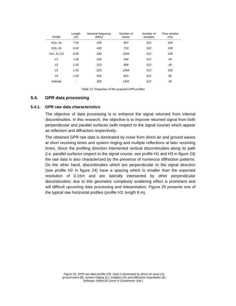
H
H
H1
5.4. GP
5.4.1. GPR
Thediscperpas rTheat stime(i.e.the On (seeresodiscwill the
Profile L
H1a, 2a
H1b, 2b
1c, 2c,3,4
V1
V2
V3
V4
Velocity
R data pro
R raw data
e objective ocontinuities. pendicular areflectors ane obtained Gshort receivines. Since th. parallel surraw data is the other h
e profile H2olution of continuities; difficult upctypical raw h
Figure ground
Length (m)
Nom
7.50
6.50
8.00
1.50
1.50
1.50
1.50
-
Table 13.
ocessing
characteris
of data procIn this resea
and parallel nd diffractorsGPR raw datng times ande profiling d
rfaces respealso charac
hand, discon2 in figure 2
0.15m andue to this
coming data horizontal pr
25. GPR raw dawave (B), system
Softwar
inal frequency (MHz)
430
430
430
265
313
525
420
300
. Properties of th
stics
cessing is tarch, the objsurfaces (w
s respectivelya is dominatd system rindirection inteect to the sigcterized by tntinuities wh24) have a d are lategeometric cprocessing
rofiles (profil
ata (profile H3). Dm ringing (C), mure: Reflex2D Quic
Number of traces
907
719
1094
546
804
1094
803
1451
he acquired GPR
to enhance jective is to ith respect ty. ted by noise
nging and mersected vernal course, sthe presencehich are perspacing wh
erally interscomplexity sand interpre
le H3, length
Data is dominateultiples (D) and dck ® (Sandmeier
Number ofsamples
512
512
512
512
512
512
512
512
profiles
the signal improve ret
to the signal
e from directultiple reflecrtical disconsee profile He of numerorpendicular hich is smalsected by scattering eetation. Figuh 8 m).
d by direct air wadiffraction hyperbr Soft.)
f Time windo(ns)
100
100
100
40
40
100
80
40
returned frourned signa course) wh
t air and groctions at latetinuities alo
H1 and H3 inous diffractioto the signaler than the
other perffect is prom
ure 25 prese
ave (A),
bolas (E).
ow
om internal l from both
hich appear
und waves er receiving ng its path n figure 24) n patterns. al direction e expected rpendicular minent and ents one of
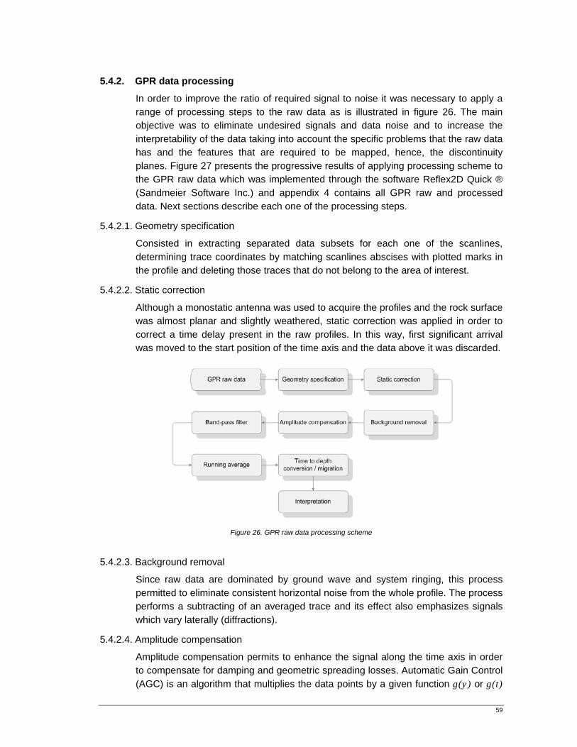
59
5.4.2. GPR data processing
In order to improve the ratio of required signal to noise it was necessary to apply a range of processing steps to the raw data as is illustrated in figure 26. The main objective was to eliminate undesired signals and data noise and to increase the interpretability of the data taking into account the specific problems that the raw data has and the features that are required to be mapped, hence, the discontinuity planes. Figure 27 presents the progressive results of applying processing scheme to the GPR raw data which was implemented through the software Reflex2D Quick ® (Sandmeier Software Inc.) and appendix 4 contains all GPR raw and processed data. Next sections describe each one of the processing steps.
5.4.2.1. Geometry specification
Consisted in extracting separated data subsets for each one of the scanlines, determining trace coordinates by matching scanlines abscises with plotted marks in the profile and deleting those traces that do not belong to the area of interest.
5.4.2.2. Static correction
Although a monostatic antenna was used to acquire the profiles and the rock surface was almost planar and slightly weathered, static correction was applied in order to correct a time delay present in the raw profiles. In this way, first significant arrival was moved to the start position of the time axis and the data above it was discarded.
Figure 26. GPR raw data processing scheme
5.4.2.3. Background removal
Since raw data are dominated by ground wave and system ringing, this process permitted to eliminate consistent horizontal noise from the whole profile. The process performs a subtracting of an averaged trace and its effect also emphasizes signals which vary laterally (diffractions).
5.4.2.4. Amplitude compensation
Amplitude compensation permits to enhance the signal along the time axis in order to compensate for damping and geometric spreading losses. Automatic Gain Control (AGC) is an algorithm that multiplies the data points by a given function g(y) or g(t)
60
respectively. g(t) function is expressed as: g(t)=exp(b*t) with b=b'*v/8.69. A propagation velocity v=0.12 m/ns and an attenuation b'= 3 dB/m (Daniels, 1996) were assumed to be constant along the signal path.
5.4.2.5. Band-pass filtering
A band-pass Butterworth (low pass and high pass filtering) was used in order to filtrate low and high frequency noise in time domain. The lower and higher cut-off frequencies for the 400 MHz centre frequency were set at 100 MHz and 600 MHz respectively (Davis and Annan, 1989).
5.4.2.6. Running average
This algorithm suppresses trace dependent noise; hence, its effect is to emphasize horizontally coherent energy corresponding to reflectors. The running average was preformed over a chosen value of 10 traces for each time step. Above this value, diffractors become unclear and lower values did not improve the data.
5.4.2.7. Time to depth conversion and migration
The objective of time to depth conversion and migration process is to trace back the reflection and diffraction energy to their source location (since zero offset sections often does not represent their true location). Time to depth conversion and migration was performed based on a propagation velocity v = 0.12 m/ns (see section 5.3) which was assumed to be constant within the rock mass. A 2D fk-migration was performed. Within the fk-range (frequency-wave number range) a variable transform is done based on a constant propagation velocity (frequency is transformed onto the vertical wave number). The x-t data is transformed into the f-k-range. After having done the transformation the migration process will be done and after that, the back transformation into the x-t-range is performed.
5.5. Results interpretation
Once each horizontal and each vertical profile were processed, the next step is to interpret them in order to map the features of interest, hence, the discontinuity surfaces. While performing interpretation it is important to consider the GPR survey conditions, field observations, and raw data characteristics. The following processing schema was applied: Geometrical parameters which are required to be mapped. The objective is to
determine location, orientation, spacing and persistence of different discontinuity sets present within the rock mass (see section 5.2.2)
Maximal resolution: As was stated in section 5.2.4, the maximal expected resolution is around 0.15 m (in depth) and 0.50 m (lateral resolution at 5 m depth). Is important to note that reflectors closer than 0.15 m can not be correctly determined. This is the case of discontinuity set J1 (set spacing = 0.07 m) and J3 (persistence along strike = 0.07 cm), see section 5.5.2.

Figs
baave
d
Relativdirectisub-hovariessomet
Next secpresent in
gure 27. Progressection (profile H3ackground removrage and d) Time
define negative an
ve orientatioon of propaorizontal an and hence,times they a
tions presen each one o
ssive results of ap3). a) Raw data, val, c) amplitude e to depth convend positive pulse
on of reflectiagation of thnd 1 oblique, depending ppear as ref
nt a discusof the proces
pplying processib) Geometry specompensation, d
ersion and migrates and colour inte
ing and refrae GPR signe discontinuon the GPR
flectors and
ssion about ssed profiles
ing scheme to a ecification, staticd) band-pass filtetion. Blues/greenensity is a functio
acting discoal. The rock
uity sets, thR profiling orsometimes
the differes.
typical horizontac correction, and ering, e) Runningns and reds/violeon of amplitude.
ntinuities wik mass has e dip directrientation it as diffractor
ent heteroge
al
g ets
th respect to4 sub-vertiction of this is supposed
rs.
eneities that
o the cal, 1
sets d that
t are
62
5.5.1.1. Horizontal profile H2a
This profile was acquired along the scanline 1 (see figure 28). Its length is 7.5 m; maximal penetration depth is around 5 m, maximal depth resolution 0.15 m and maximal lateral resolution 0.50 (at 5 m depth). It presents a series of persistent and repetitive series of closely spaced parallel heterogeneities along the profile direction that can be due either to a remaining ringing effect that could not be eliminated after the applied processing schema, or to a reflection from discontinuity set J1 (orientation 170/86) which is very dense (normal set spacing = 0.07 m), has a small gap (less than 1cm) and has washed clay as infill. Based on scanline observations, it can be noticed that refractors a1 and a2 correspond to those discontinuities located at the abscise 0.14m (orientation 252/89) and 1.48 m (orientation 081/65). Refractor b correspond to the discontinuity located at abscise 3.69 m (orientation 254/70), and refractor c correspond to the discontinuity located at abscise 6.17m (orientation 268/80). The strike direction observed in the profile is consistent with such orientations and the persistence (along strike direction) of these discontinuities in appearance is greater than the penetration depth of the GPR signal. Refractor d corresponds to side effects (this refraction pattern is caused by the corner at the end of the scan-line 1, see figure 28). Other refractors are difficult to be interpreted as persistent discontinuities since they do not keep a constant pattern along depth.
5.5.1.2. Horizontal profile H2b
This profile was acquired along the scanline 2 (see figure 28). Its length is 6.5 m; maximal penetration depth is around 5 m, maximal depth resolution 0.15 m and maximal lateral resolution 0.50 (at 5 m depth). It presents a series of persistent and repetitive series of closely spaced parallel heterogeneities along the profile direction that indeed are due to a remaining ringing effect that could not be eliminated after the applied processing schema. This last since discontinuity sets J2, J3, J4 and J6 (which would act as reflectors in this case) have not such small spacing as that observed the profile along its depth. Refractors f and i correspond to side effects (caused by the corners at the beginning and at the end of the scan-line 2, see figure 28) and reflectors g and h correspond to superficial voids. Neither, discontinuity location, spacing, orientation nor persistence can be clearly defined from this profile.
5.5.1.3. Horizontal profile H3
This profile was acquired along the scanline 3 (see figure 29). Its length is 8.0 m; maximal penetration depth is around 6 m, maximal depth resolution 0.15 m and maximal lateral resolution 0.50 (at 5 m depth). It also presents a series of persistent and repetitive series of closely spaced parallel heterogeneities along the profile direction that can be due either to a remaining ringing effect that could not be eliminated after the applied processing schema, or to a reflection from discontinuity set J1.
63
Based on scanline observations, it can be noticed that refractor j corresponds to side effects (caused by the corner at the beginning of the scan-line 3, see figure 29). Refractors k and l correspond to those discontinuities located at abscises 14.68 m (orientation 252/88) and 16.42 m (orientation 250/89) and refractor m corresponds to the discontinuity at 18.47 m (orientation 79/72). The strike direction observed in the profile is consistent with such orientations and the persistence (along strike direction) of these discontinuities in appearance is greater than the penetration depth of the GPR signal.
5.5.1.4. Horizontal profile H4
This profile was acquired along the scanline 3 (see figure 29). Its length is 8.0 m; maximal penetration depth is around 2 m, and maximal depth resolution 0.15 m. Its objective was to corroborate the observations of profile H3. It also presents a series of persistent and repetitive series of closely spaced parallel heterogeneities along the profile direction that can be due either to a remaining ringing effect that could not be eliminated after the applied processing schema, or to a reflection from discontinuity set J1 which is very dense (set spacing = 0.07 m). This profile permits to determine more accurately the location of the refractors observed in the profile H4 and to observe in a better way the reflection patterns of discontinuity set J1, hence it is possible to verify its persistence and orientation of discontinuity set J1. Set spacing could not be accurately determined because of the limited resolution of the GPR survey.
5.5.1.5. Vertical profile V1
This profile was acquired in a perpendicular direction respect to the scanline 1, at abscise 3.5 m (see figure 28). Its height is 1.5 m; penetration depth is around 2 m, maximal depth resolution 0.15 m. It also present a series of persistent and repetitive series of closely spaced parallel heterogeneities along the profile direction that can be due either to a remaining ringing effect that could not be eliminated after the applied processing schema, or to a reflection from discontinuity set J1 which is very dense (set spacing = 0.07 m). No refractors are observed. From the reflection pattern is possible to verify the persistence and orientation of discontinuity set J1. Its persistence along strike and dip its grater than the profiled section and its orientation follows that observed on surface. Set spacing could not be accurately determined because of the limited resolution of the GPR survey.
5.5.1.6. Vertical profile V2, V3 and V4
These profiles were acquired in a perpendicular direction respect to the scanline 3 at abscises 14.5, 16.0 and 18.0 m (see figure 29). Their height is 1.5 m; penetration depth is around 2 m, maximal depth resolution 0.15 m. They also present a series of persistent and repetitive series of closely spaced parallel heterogeneities along the profile direction that can be due either to a remaining ringing effect that could not be eliminated after the applied processing schema, or to a reflection from discontinuity set J1 which is very dense (set spacing = 0.07 m).
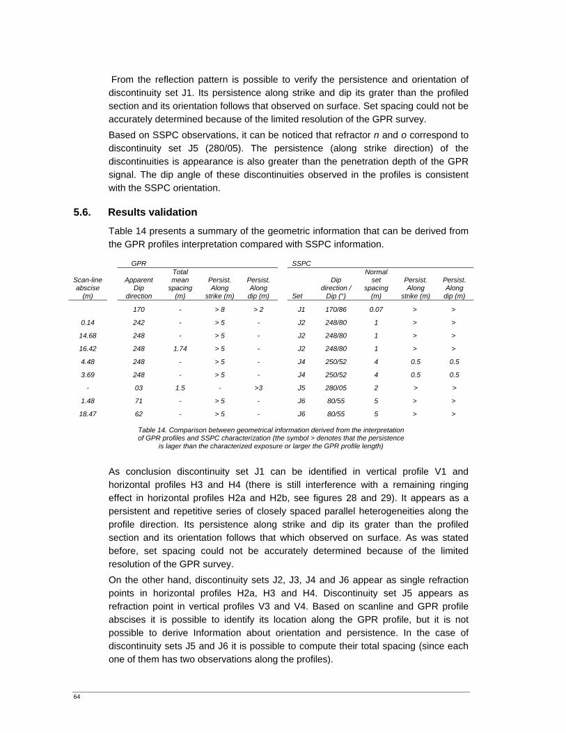
64
From the reflection pattern is possible to verify the persistence and orientation of discontinuity set J1. Its persistence along strike and dip its grater than the profiled section and its orientation follows that observed on surface. Set spacing could not be accurately determined because of the limited resolution of the GPR survey. Based on SSPC observations, it can be noticed that refractor n and o correspond to discontinuity set J5 (280/05). The persistence (along strike direction) of the discontinuities is appearance is also greater than the penetration depth of the GPR signal. The dip angle of these discontinuities observed in the profiles is consistent with the SSPC orientation.
5.6. Results validation
Table 14 presents a summary of the geometric information that can be derived from the GPR profiles interpretation compared with SSPC information.
GPR SSPC
Scan-line abscise
(m)
Apparent
Dip direction
Total mean
spacing (m)
Persist. Along
strike (m)
Persist. Along
dip (m) Set
Dip direction /
Dip (°)
Normal set
spacing (m)
Persist. Along
strike (m)
Persist. Along
dip (m)
170 - > 8 > 2 J1 170/86 0.07 > >
0.14
242 - > 5 - J2 248/80 1 > >
14.68
248 - > 5 - J2 248/80 1 > >
16.42
248 1.74 > 5 - J2 248/80 1 > >
4.48
248 - > 5 - J4 250/52 4 0.5 0.5
3.69
248 - > 5 - J4 250/52 4 0.5 0.5
-
03 1.5 - >3 J5 280/05 2 > >
1.48
71 - > 5 - J6 80/55 5 > >
18.47
62 - > 5 - J6 80/55 5 > >
Table 14. Comparison between geometrical information derived from the interpretation of GPR profiles and SSPC characterization (the symbol > denotes that the persistence
is lager than the characterized exposure or larger the GPR profile length) As conclusion discontinuity set J1 can be identified in vertical profile V1 and horizontal profiles H3 and H4 (there is still interference with a remaining ringing effect in horizontal profiles H2a and H2b, see figures 28 and 29). It appears as a persistent and repetitive series of closely spaced parallel heterogeneities along the profile direction. Its persistence along strike and dip its grater than the profiled section and its orientation follows that which observed on surface. As was stated before, set spacing could not be accurately determined because of the limited resolution of the GPR survey. On the other hand, discontinuity sets J2, J3, J4 and J6 appear as single refraction points in horizontal profiles H2a, H3 and H4. Discontinuity set J5 appears as refraction point in vertical profiles V3 and V4. Based on scanline and GPR profile abscises it is possible to identify its location along the GPR profile, but it is not possible to derive Information about orientation and persistence. In the case of discontinuity sets J5 and J6 it is possible to compute their total spacing (since each one of them has two observations along the profiles).
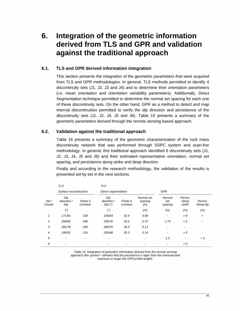
65
6. Integration of the geometric information derived from TLS and GPR and validation against the traditional approach
6.1. TLS and GPR derived information integration
This section presents the integration of the geometric parameters that were acquired from TLS and GPR methodologies. In general, TLS methods permitted to identify 4 discontinuity sets (J1, J2, J3 and J4) and to determine their orientation parameters (i.e. mean orientation and orientation variability parameters). Additionally, Direct Segmentation technique permitted to determine the normal set spacing for each one of these discontinuity sets. On the other hand, GPR as a method to detect and map internal discontinuities permitted to verify the dip direction and persistence of the discontinuity sets (J1, J2, J4, J5 and J6). Table 15 presents a summary of the geometric parameters derived through the remote sensing based approach.
6.2. Validation against the traditional approach
Table 16 presents a summary of the geometric characterization of the rock mass discontinuity network that was performed through SSPC system and scan-line methodology. In general, this traditional approach identified 6 discontinuity sets (J1, J2, J3, J4, J5 and J6) and their estimated representative orientation, normal set spacing, and persistence along strike and deep direction. Finally and according to the research methodology, the validation of the results is presented set by set in the next sections.
TLS TLS
Surface reconstruction Direct segmentation GPR
Set / Cluster
Dip direction /
Dip Fisher k constant
Dip direction /
Dip (°) Fisher k constant
Normal set spacing
(m)
Normal set
spacing
Persist. Along strike
Persist. Along dip
(°) (°) (m) (m) (m) (m)
1 171/81 159 165/83 32.4 0.08 - > 8 >
2 258/82 268 259/78 33.2 0.37 1.74 > 5 -
3 281/78 186 289/79 34.4 0.13 - - -
4 249/52 216 250/48 35.3 0.14 - > 5 -
5 - - - - - 1.5 - > 3
6 - - - - - - > 5 -
Table 15. Integration of geometric information derived from the remote sensing approach (the symbol > denotes that the persistence is lager than the characterized
exposure or larger the GPR profile length).
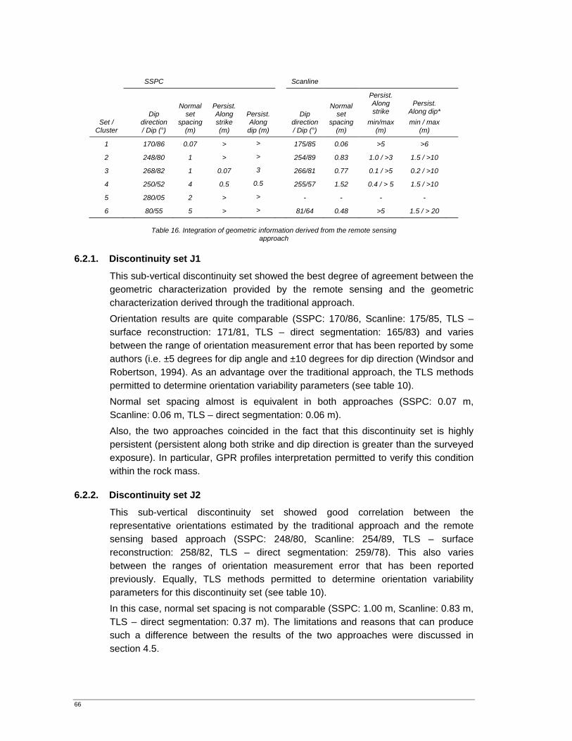
66
SSPC Scanline
Set / Cluster
Dip direction / Dip (°)
Normal set
spacing (m)
Persist. Along strike (m)
Persist. Along
dip (m)
Dip direction / Dip (°)
Normal set
spacing (m)
Persist. Along strike
min/max (m)
Persist. Along dip* min / max
(m)
1 170/86 0.07 > > 175/85 0.06 >5 >6
2 248/80 1 > > 254/89 0.83 1.0 / >3 1.5 / >10
3 268/82 1 0.07 3 266/81 0.77 0.1 / >5 0.2 / >10
4 250/52 4 0.5 0.5 255/57 1.52 0.4 / > 5 1.5 / >10
5 280/05 2 > > - - - -
6 80/55 5 > > 81/64 0.48 >5 1.5 / > 20
Table 16. Integration of geometric information derived from the remote sensing approach
6.2.1. Discontinuity set J1
This sub-vertical discontinuity set showed the best degree of agreement between the geometric characterization provided by the remote sensing and the geometric characterization derived through the traditional approach. Orientation results are quite comparable (SSPC: 170/86, Scanline: 175/85, TLS – surface reconstruction: 171/81, TLS – direct segmentation: 165/83) and varies between the range of orientation measurement error that has been reported by some authors (i.e. ±5 degrees for dip angle and ±10 degrees for dip direction (Windsor and Robertson, 1994). As an advantage over the traditional approach, the TLS methods permitted to determine orientation variability parameters (see table 10). Normal set spacing almost is equivalent in both approaches (SSPC: 0.07 m, Scanline: 0.06 m, TLS – direct segmentation: 0.06 m). Also, the two approaches coincided in the fact that this discontinuity set is highly persistent (persistent along both strike and dip direction is greater than the surveyed exposure). In particular, GPR profiles interpretation permitted to verify this condition within the rock mass.
6.2.2. Discontinuity set J2
This sub-vertical discontinuity set showed good correlation between the representative orientations estimated by the traditional approach and the remote sensing based approach (SSPC: 248/80, Scanline: 254/89, TLS – surface reconstruction: 258/82, TLS – direct segmentation: 259/78). This also varies between the ranges of orientation measurement error that has been reported previously. Equally, TLS methods permitted to determine orientation variability parameters for this discontinuity set (see table 10). In this case, normal set spacing is not comparable (SSPC: 1.00 m, Scanline: 0.83 m, TLS – direct segmentation: 0.37 m). The limitations and reasons that can produce such a difference between the results of the two approaches were discussed in section 4.5.
67
On the other hand, GPR survey permitted to verify its persistence within the rock mass. Also, the two approaches coincided in the fact that this discontinuity set is persistent along strike direction (persistence is larger than the surveyed exposure).
6.2.3. Discontinuity set J3
This sub-vertical discontinuity set showed good correlation between the representative orientations estimated by the traditional approach and the remote sensing based approach (SSPC: 268/82 and Scanline: 266/81, TLS – surface reconstruction: 281/78, TLS – direct segmentation: 289/79). This also varies between the ranges of orientation measurement error that has been reported previously. Equally, TLS methods permitted to determine orientation variability parameters for this discontinuity set (see details on table 10). In this case, normal set spacing is not comparable (SSPC: 1.00 m, Scanline: 0.77 m, TLS – direct segmentation: 0.13 m). The limitations and reasons that can produce such a difference between the results of the two approaches were discussed in section 4.5. In this case, remote sensing approach did not permit to determine the persistence of this discontinuity set.
6.2.4. Discontinuity set J4
This oblique discontinuity set showed good correlation between the representative orientations estimated by the traditional approach and the remote sensing based approach (SSPC: 250/52, Scan-line: 255/57, TLS – surface reconstruction: 249/52, TLS – direct segmentation: 250/48). This also varies between the ranges of orientation measurement error that has been reported previously. Equally, TLS methods permitted to determine orientation variability parameters for this discontinuity set (see details on table 10). Also, normal set spacing is not comparable (SSPC: 4.00 m, Scan-line: 1.52, TLS – direct segmentation: 0.14 m). The limitations and reasons that can produce such a difference between the results of the two approaches were discussed in section 4.5. On the other hand, GPR survey permitted to verify its persistence within the rock mass. Also, the two approaches coincided in the fact that this discontinuity set is persistent along strike direction (persistence is larger than the surveyed exposure).
6.2.5. Discontinuity set J5
This sub-horizontal discontinuity set was not recognized by the remote sensing approach. The limitations of the TLS methods which impeded its identification were discussed on section 4.4.1.2. On the other hand, through interpretation of the GPR profiles and taking into account the previous SSPC observations, it was possible to identify some of the horizontal discontinuities which belong to this discontinuity set and to determine a set spacing of 1.5 m and its persistence along dip direction.
6.2.6. Discontinuity set J6
This oblique discontinuity set was not recognized by the remote sensing approach. The limitations of the TLS methods which impeded its identification were also
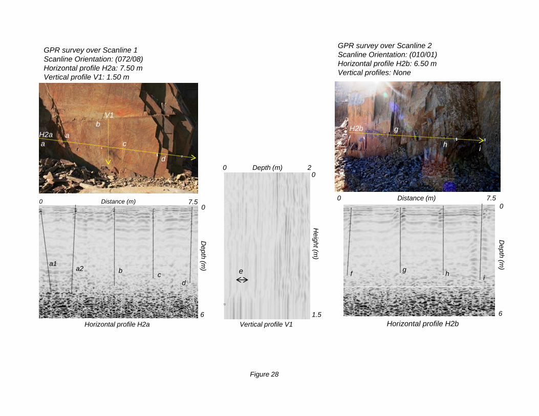
GPR survey over Scanline 1Scanline Orientation: (072/08)Horizontal profile H2a: 7.50 mVertical profile V1: 1 50 m
GPR survey over Scanline 2 Scanline Orientation: (010/01)Horizontal profile H2b: 6.50 mVertical profiles: NoneVertical profile V1: 1.50 m
bg
V1
H2ba
c
d0 2Depth (m)
0
fg
h i
H2aH2b
a
0 7.50
Distance (m)
He
0 7.50
Distance (m)
a2 b cd
Depth (m
)
eight (m)
e f g h i
Depth (m
)a1
6 1.5Horizontal profile H2a Vertical profile V1
6Horizontal profile H2b
Figure 28
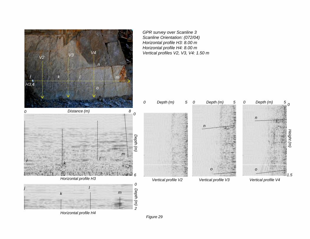
GPR survey over Scanline 3Scanline Orientation: (072/04)Horizontal profile H3: 8.00 mpHorizontal profile H4: 8.00 mVertical profiles V2, V3, V4: 1.50 m
nV2 V3 V4
0
j k l m
o
0 5Depth (m) 00 5Depth (m) 0 5Depth (m)
H3,4
0
80 Distance (m)
D
0
n
n
0
HeiD
epth (m)
jk
lm
ight (m)
6Horizontal profile H3
0
Dep
o o
jk
lm
1.5Vertical profile V2 Vertical profile V3 Vertical profile V4
Horizontal profile H42
pth (m)
Figure 29
68
discussed on section 4.4.1.2. Similarly to discontinuity set J5, through interpretation of the GPR profiles and taking into account the previous SSPC observations, it was possible to identify some of the discontinuities which belong to this discontinuity set and to determine its persistence along strike.
6.3. General observations
6.3.1. Number of discontinuity sets
SSPC method which (theoretically) avoids sampling biases for orientation and limited length of scanline surveys (see section 2.3.1) determined six discontinuity sets within the rock mass. Due to orientation bias and its limited length (see section 3.2.2.2); the scanline method determined five discontinuity sets (J1, J2, J3, J4 and J6). TLS methods (both surface reconstruction and direct segmentation techniques) were able to determine four sets (J1, J2, J3 and J4). Discontinuity sets J5 and J6 were not identified because of their relative orientation respect to the slope surface and respect to the laser beam (see section 4.4.1.2)
6.3.2. Discontinuity sets orientation
SSPC and line-scan survey methods could involve both human bias and instrument error when determining the orientation of the discontinuity sets. On the other hand, due to the large quantity of orientation data derived from TLS methods, the identification of such individual sets, as well as their mean orientation and orientation variability could be performed objectively based on their statistical orientation distributions.
6.3.3. Normal discontinuity set spacing
Making an exception for the discontinuity set 1; the normal set spacing results derived from each approach are not comparable. This is due to the fact that the three approaches are very different and hence their results. The SSPC system (which is based on the rapid face mapping methodology) trended to overestimate this parameter. The scanline survey, which was concentrated on acquiring discontinuity information over a 2D surface along a single direction with a limited length trends to underestimate the normal set spacing. TLS – direct segmentation technique, represents the discontinuity network as a collection of parameterized planes in a 3D space. As was discussed in section 4.5, because of local variations, a single discontinuity surface can be over-segmented and generate several smaller planes. The normal set spacing between these close planes is very small and hence the normal set spacing is underestimated by this method. GPR survey has some limitations than scanline. GPR profiles were acquired along single orientations and along limited lengths. In addition, the GPR limited resolution and the relative orientation of the profiling direction respect to discontinuities reduced its effectiveness while determining discontinuities location and spacing.
69
6.3.4. Discontinuity sets persistence
For the case of the discontinuity set J1, the GPR method showed good correlation with the persistence determined by SSPC system and scanline survey. For the other discontinuity sets, it was not possible to verify their persistence within the rock mass. This was due to the limited number of discontinuities that could be objectively identified while interpreting the GPR profiles.
7. Conclusions
The individual results and the integrated analysis of the geometrical information derived from Terrestrial Laser Scanner and Ground Penetrating Radar showed a reasonable degree of correlation with the results of the traditional approach and demonstrated to be an attractive way of complement such information in order to reduce the degree of uncertainty about the geometrical characteristics of the discontinuity network of a rock mass. Along this research, the specific added value of the remote sensing methods is that they permitted: a) To identify in an objective way four of the six discontinuity sets present within the rock mass and to derive its mean orientation and variability parameters based on the orientation statistics of the large quantity of orientation data derived from the TLS survey, b) To determine the persistence of the discontinuities within the rock mass, and c) The acquisition and integrated analysis of geometric data through both, traditional (SSPC and scan-line) and remote sensing approaches (Terrestrial Laser Scanner and Ground Penetrating Radar) showed to be a convenient way to characterize a rock mass. The geometric parameters derived from the two approaches permitted to gather information, contrast observations and validate results. The principles, assumptions and data process methods involved in both Terrestrial Laser Scanner and Ground Penetrating Radar techniques determines the degree of consistency of their results. Along this research, it has been recognized that it is important to consider the following issues.
7.1. Terrestrial Laser Scanner method
The assumption behind TLS methods is that the geometry of the visible rock mass surface has a relation with the geometry of the discontinuity network within the rock mass. This is not necessary true in all rock mass exposures.
In discontinuity network modeling approaches, each discontinuity is considered as relatively simple feature (i.e. a plane with a given orientation, spacing and persistence). Surface Reconstruction and Direct Segmentation methods to derive geometric information showed to be influenced by local variations (i.e. large scale roughness) within the discontinuity plane (see sections 4.4 and 4.5).
The identification of discontinuity sets is based on the orientation distribution of the discontinuities within the rock mass assuming a Fisher distribution. As it has
70
been discussed in section 2.6.2.3, other situations may also be present in a rock mass; however the analysis of those situations has not be integrated in these methods.
As it has been discussed in section 2.6, discontinuity spacing, discontinuity density, trace length and persistence behaviour is usually treated using statistical methods based on the central limit theorem. Such approaches has been developed to analyse discontinuity data that is acquired over 2D exposures using sampling window or scan-line techniques. On the other hand TLS methods are capable to provide a discontinuity network model represented by finite planes in a 3D space, the inconsistencies that were found while characterizing discontinuity spacing in such a model suggest that appropriate methodologies must to be developed to derive geometrical parameters of such 3D models.
7.2. Ground penetrating radar
The assumption behind GPR method is that the heterogeneities present in the subsurface profiles represent internal discontinuities. As was discussed along section 5.5 the interpretation of such heterogeneities becomes difficult when undesired signals appear in the profiles (i.e. multiples and ringing effect).
A limitation of the present research is the limited number of acquired profiles. Hence, every single profile had to be correlated with a surface observation (through scanline). Ideally, a complete determination of the discontinuities would require a set of close parallel and perpendicular GPR profiles as well as compound processing and interpretation methodology. In this way a representation of the 3D discontinuity network can be obtained through the correlation of discontinuity signatures of each profile with those from the nearest one.
On the other hand, as is discussed in section 5.2.4, the survey conditions (limited vertical and horizontal resolution) and the the relative complexity of the discontinuity network constrained GPR performance (reduced depth penetration, scattering and multi-path effects). This effects has been also confirmed by other authors (see Grandjean and Gourry, 1996). The use of higher frequencies would permit to obtain a better resolution (but with an inferior penetration depth).
71
References
Ang, A. H. S. and Tang, W. (1975) Probability Concepts in Engineering Planning and Design, New York.
Ayalew, L., Reik, G. and Busch, W. (2002) Characterizing weathered rock masses--a geostatistical approach. International Journal of Rock Mechanics and Mining Sciences, 39, 105-114.
Baecher, G. B. and Lanney, N. A. (1978) Trace lenghts biases in joint surveys. In 19 U.S. Symp. on Rock Mechanics, Vol. 1 U.S., pp. 56-65.
Benjamin, J. R. and Cornell, C. A. (1970) Probability, Statistics, and Desicion for Civil Engineers, New York.
Bentley, J. L. (1975) Multidimensional binary search trees used for associative searching. Communications of the ACM, 18, 509 - 517.
Bezdek, J. C. (1981) Pattern recognition with fuzzy objective function algorithms, New York. Bieniawski, Z. T. (1989) Engineering Rock Mass Classification, New York. Billaux, D., Chiles, J. P., Hestir, K. and Long, J. (1989a) Three-dimensional statistical
modelling of a fractured rock mass--an example from the Fanay-Augeres mine. International Journal of Rock Mechanics and Mining Science & Geomechanics Abstracts, 26, 281-299.
Billaux, D., Chiles, J. P., Hestir, K. and Long, J. (1989b) Three-dimensional statistical modelling of a fractured rock mass, an example from the Fanay-Augeres mine. International Journal of Rock Mechanics and Mining Science & Geomechanics Abstracts, 26, 281-299.
Bingham, C. (1964) Distributions on the sphere and on the projective plane. Yale University, New Haven, Conetticut. .
Brady, B. H. G. and Brown, E. T. (2004) Rock Mechanics: For Underground Mining, Springer.
Bridges, M. C. (1975) Presentation of fracture data for rock mchanics. In 2nd Australia - New Zealand conference on GeomechanicsBrisbane, pp. 144 - 148.
British Standard Institution, B. (1999) 5930:1999 Code of practice for site investigations, BSI, London.
Carr, J. C., Beatson, R. K., Cherrie, J. B., Mitchell, T. J., Fright, W. R., McCallum, B. C. and Evans, T. R. (2001) Reconstruction and Representation of 3-D Objects with Radial Basis Functions. In ACM SIGGRAPHLos Angeles, CA, pp. 67-76.
Carr, J. C., Beatson, R. K., Cherrie, J. B., Mitchell, T. J., Fright, W. R., McCallum, B. C. and Evans, T. R. (2003) Smooth surface reconstruction from noisy range data. In ACM GRAPHITE 2003Melbourne, Australia, pp. 119 -126.
Chiles, J. P. (1989) Fractal and geostatistical methods for modeling of a fracture network : Chiles, J P Math Geol V20, N6, Aug 1988, P631-654. International Journal of Rock Mechanics and Mining Science & Geomechanics Abstracts, 26, A134.
Coggan, J. S., Wetherelt, A., Gwynn, X. P. and Flynn, Z. N. (2007) Comparison of hand-mapping with remote data capture systems for effective rock mass characterisation. In Congress of the International Society for Rock Mechanics - the second half century of rock mechanics, Vol. 1 (Ed, Francis, T. a.) Lisbon, Portugal, pp. 201 - 205.
Davis, J. C. (1986) Statistics and Data Analysis in Geology, John Wiley & Sons, Singapore. Davis, J. C. (2002) Statistics and Data Analysis in Geology, John Wiley & Sons, Singapore. Davis, J. L. and Annan, A. P. (1989) Ground penetrating radar for high resolution mapping of
soil and rock stratigraphy. Geophysical Prospecting, 37, 531-551. Deparis, J. and Garambois, S. (2006) Fracture imaging and characterization from apvo gpr
data. In 11th Int. Conf. on Ground Penetrating RadarColumbus, Ohio, USA. Deparis, J., Garambois, S. and Hantz, D. (2007) On the potential of Ground Penetrating
Radar to help rock fall hazard assessment: A case study of a limestone slab, Gorges de la Bourne (French Alps). Engineering Geology, 94, 89-102.
72
Ehlen, J. (2000) Fractal analysis of joint patterns in granite. International Journal of Rock Mechanics and Mining Sciences, 37, 909-922.
Einstein, H. H. (1993) Modern developments in discontinuity analysis the persistence discontinuity problem. In Comprehensive rock engineering, Vol. 3 (Ed, Pergamon) Oxford, pp. 215 - 239.
Fisher, R. (1953) Dispersion on a sphere. . In Royal Society London, Vol. A217, pp. 295-305. Fröhlich, C. (2004) Terrestrial laser scanning, New perspectives in 3D surveying.
International Archives of Photogrammetry, Remote Sensing and Spatial Information Sciences, 36.
Gath, I. and Geva, A. B. (989) Unsupervised optimal fuzzy clustering. IEEE Trans. Pattern Anal. Machine Intell., 11, 773-781.
Goodman, R. E. (1989) Introduction to rock mechanics, Wiley & Sons, New York. Goodman, R. E. and Shi, G. (1985) Block Theory and Its Application to Rock Engineering,
Prentice-Hall, New Jersey. Grandjean, G. and Gourry, J. C. (1996) GPR data processing for 3D fracture mapping in a
marble quarry (Thassos, Greece). Journal of Applied Geophysics, 36, 19-30. Hack, H. R. G. K. (1998) Slope stability probability classification. International Institute for
Aerospace Survey and Earth Sciences (ITC), Enschede, pp. 258. Harrison, J. P. (1992) Fuzzy objective functions applied to the analysis of discontinuity
orientation data. In Eurock 92, pp. 25-30. Hobbs, B. E. (1993) The Significance of Structural Geology in Rock Mechanics. Hoek, E. and Bray, J. W. (1981) Rock slope engineering, The Institution of Mining and
Metallurgy, London. Huang, S. L., Oelfke, S. M. and Speck, R. C. (1992) Applicability of fractal characterization
and modelling to rock joint profiles. International Journal of Rock Mechanics and Mining Science & Geomechanics Abstracts, 29, 89-98.
Hudson, H. (1989) Engineering Rock Mechanics, London. ISRM (1981) Rock characterization, testing and monitoring, ISRM suggested methods,
Oxford. Jimenez-Rodriguez, R. and Sitar, N. (2006) A spectral method for clustering of rock
discontinuity sets. International Journal of Rock Mechanics and Mining Sciences, 43, 1052-1061.
Kalenchuk, K. S., Diederichs, M. S. and McKinnon, S. (2006) Characterizing block geometry in jointed rockmasses. International Journal of Rock Mechanics and Mining Sciences, 43, 1212-1225.
Kemeny, J. (2003) Estimating three-dimensional rockdiscontinuity orientation from digital images of fracture traces. Computers & Geosciences, 29.
Kemeny, J. and Donovan, J. (2005) Rock mass characterization using LIDAR and automated point cloud processing. Ground Engineering, 26.
Kulatilake, A. E. (1985) Estimation of mean trace length of discontinuities : Kulatilake, P H S W; Wu, T H Rock Mech V17, N4, Oct-Dec 1984, P215-232. International Journal of Rock Mechanics and Mining Science & Geomechanics Abstracts, 22, A105.
Kulatilake, P. H. S. W., Um, J.-g., Wang, M., Escandon, R. F. and Narvaiz, J. (2003) Stochastic fracture geometry modeling in 3-D including validations for a part of Arrowhead East Tunnel, California, USA. Engineering Geology, 70, 131-155.
Kulatilake, P. H. S. W., Wathugala, D. N. and Stephansson, O. (1993) Joint network modelling with a validation exercise in Stripa mine, Sweden. International Journal of Rock Mechanics and Mining Science & Geomechanics Abstracts, 30, 503-526.
La Pointe, P. R. and Hudson, J. A. (1985) Characterization and interpretation of rock mass joint patterns. Geol. Soc. of America, 199.
Lemy, F. and Hadjigeorgiou, J. (2003) Discontinuity trace map construction using photographs of rock exposures. International Journal of Rock Mechanics and Mining Sciences, 40, 903-917.
Parasnis, D. S. (1997) Principles of applied geophysics, Chapman & Hall, London etc.
73
Porsani, J. L., Sauck, W. A. and Junior, A. O. S. (2006) GPR for mapping fractures and as a guide for the extraction of ornamental granite from a quarry: A case study from southern Brazil. Journal of Applied Geophysics, 58, 177-187.
Priest, S. (1985) Hemispherical projection methods in rock mechanics, Allen & Unwin, London; Boston.
Priest, S. D. (1993) Discontinuity analysis for rock engineering, Chapman & Hall, London, New York.
Priest, S. D. and Hudson, J. A. (1981) Estimation of discontinuity spacing and trace length using scanline surveys. International Journal of Rock Mechanics and Mining Science & Geomechanics Abstracts, 18, 183-197.
Rafiee, A. and Vinches, M. (2007) Application of geostatistical characteristics of rock mass fracture systems in 3D model generation. International Journal of Rock Mechanics and Mining Sciences, In Press, Corrected Proof.
Reynolds, J. M. (1997) introduction to applied and environmental geophysics, Wiley & Sons, Chichester etc.
Robertson, A. (1970) The interpretation of geologic factors for use in slope theory. In Proc. Symp. on the Theoretical Background to the Planning of Open Pit Mines with Special Reference to Slope StabilityJohannesburg, South Africa, pp. 55-71.
Roncella, R. and Forlani, G. (2005) Extraction of planar patches from point clouds to retrieve dip and dip direction of rock discontinuities. In ISPRS WG III/4, V/3 Workshop “Laser scanning 2005”Enschede, The Netherlands.
Rotonda, T., Marsella, M., Lizzadro, L. and Ricca, A. (2007) Analysis of laser scanner data collected during a survey of faces in a rock quarry. In Int. Congr. on Rock MechanicsLisbon.
Sen, Z. and Kazi, A. (1984) Discontinuity spacing and RQD estimates from finite length scanlines. International Journal of Rock Mechanics and Mining Science & Geomechanics Abstracts, 21, 203-212.
Slob, S., Hack, H. R. G. K., Feng, Q., Roshoff, K. and Turner, K. (2006) Fracture mapping using 3D laser scanning techniques.
Slob, S., Hack, H. R. G. K., van Knapen, B. and Kemey, J. (2004) Automated identification and characterisation of discontinuity sets in outcropping rock masses using 3D terrestrial laser scan survey techniques. In: Proceedings of the ISRM regional symposium EUROCK 2004 and 53rd Geomechanics colloquy : Rock engineering and practice, October 7-9, 2004 Salzburg, Austria. / ed. by W. Schubert. Essen; Verlag Glückauf, 2004. ISBN 3-77-395995-8 pp. 439-443.
Slob, S., Hack, H. R. G. K., van Knapen, B., Turner, K. and Kemeny, J. (2005) Method for Automated Discontinuity Analysis of Rock Slopes with 3D laser scanner. Journal of the Transportation Research Board, 1913.
Slob, S. and van Knapen, B. (2005) Rock mass characterization with 3D laser scanner. Ingeokring Newsletter, 12.
Slob, S. and van Knapen, B. (2006) Identification and characterisation of rock mass discontinuity sets using 3D laser scanning. IAEG, The Geological Society of London.
Stevens, K. M., Lodha, G. S., Holloway, A. L. and Soonawala, N. M. (1995) The application of ground penetrating radar for mapping fractures in plutonic rocks within the Whiteshell Research Area, Pinawa, Manitoba, Canada. Journal of Applied Geophysics, 33, 125-141.
Toshioka, T., Tsuchida, T. and Sasahara, K. (1995) Application of GPR to detecting and mapping cracks in rock slopes. Journal of Applied Geophysics, 33, 119-124.
Vosselman, G., Gorte, B. G. H., Sithole, G. and Rabbani, T. (2005) Recognising structure in laser scanner point clouds. In International Archives of the Photogrammetry, Remote Sensing and Spatial Information Sciences. ISPRS WG III/4, V/3 Workshop “Laser scanning 2005”.Enschede, The Netherlands.
Wathugala, D. N., Kulatilake, P. H. S. W., Wathugala, G. W. and Stephansson, O. (1990) A general procedure to correct sampling bias on joint orientation using a vector approach. Computers and Geotechnics, 10, 1-31.

74
Windsor, C. R. and Robertson, W. V. (1994) Rock Mass Formulation. Wines, D. R. and Lilly, P. A. (2002) Measurement and analysis of rock mass discontinuity
spacing and frequency in part of the Fimiston Open Pit operation in Kalgoorlie, Western Australia: a case study. International Journal of Rock Mechanics and Mining Sciences, 39, 589-602.
Xie, X. L. and Beni, G. A. (1991) A validity measure for fuzzy clustering. IEEE Trans. Pattern Anal. Machine Intell., 13, 841-847.
Yang, Z. Y. and Di, C. C. (2001) A directional method for directly calculating the fractal parameters of joint surface roughness. International Journal of Rock Mechanics and Mining Sciences, 38, 1201-1210.
Zadeh, L. A. (1965) Fuzzy sets. Information Control, 8, 338 – 353. Zhang, Z., Zhenga, S. and Zhana. (2004) Digital terrestrial photogrammetry with photo total
station. International Archives of the Photogrammetry, Remote Sensing and Spatial Information Sciences, 35.
Zillur Rahman, M. (2005) Deriving roughness characteristics of rock mass discontinuities from terrestrial laser scan data. ITC, Enschede, pp. 100.

Appendix 1


Appendix 2
International Institute for Geo‐Information Science and Earth Observation Exposure characterizationApplied Earth Sciences Department Scan line logging sheetGeo‐engineering specialization
LOGGED BY: Mark DATE: 13/09/2007 TIME: 13:30 h EXPOSURE No: 2 Accessibility: poor/fair/good SCANLINE
WEATHER CONDITIONS LOCATION: Montegaggio (Albiano, Italy) SLOPE FACE : 1 Dip direction 166 Scan line no. 1 Length 7.15
Sun: Coordinates: Northing: Size total exposure (m) l: 25.30 h: 20 d: 1 Dip 87 Dip direction O72
Rain: Easting: Mapped on this form (m) l:7.15 h: 20 d: 1 Height 20 Dip O8
DIS SPA (t/s/n) DDN (000‐360) DIP (00‐90) LEN (t/s) (m) TTN (o/r/j) BTN (o/r/j) LEN (t/s) (m) TTN (o/r/j) BTN (o/r/j) wavy
slightly wavy
curved
slightly curved
straight
rough step
ped
smoo
th stepp
ed
polishe
d step
ped
rough un
dulatin
g
smoo
th und
ulating
polishe
d un
dulatin
g
rough plan
ar
smoo
th plana
r
polishe
d plan
ar
coarse
med
ium
fine
coarse
med
ium
fine *
1 0.14 252 89 >3 j o >10 j O X X X
2 0.26 258 63 0.1 j o 1.3 j O X X X
3 0.87 256 80 0.1 j o 0.58 j O X X X
4 0.93 256 80 0.1 j o 0.58 j O X X X
5 1.03 256 80 0.1 j o 0.4 j X X X
6 1.08 256 80 0.1 j o 0.15 j O X X X
7 1.18 256 80 0.1 j o 0.2 j O X X X X
8 (m) 1.48 81 65 >5 (i) j o >20 j O X X
9 2.4 84 60 >5 (i) j o 1.5 j O X X X
10 2.67 80 85 2 (i) j o 1.5 j O X X X
11 2 (e) 261 80 >5 (i) j o 10 j O X X X
12 3 254 80 >5 (i) j o 10 j O X X X
13 2.7 79 60 >5 (i) j o 1.5 j O X X X
14 3.27 267 77 0.50 (i) j o 1.5 j O X X X
15 3.49 254 76 0.50 (i) j o 2 j O X X X
16 3.69 254 70 0.50 (i) j o 3 j O X X X
17 4.34 76 87 1.00 (i) j o 2 j O X X X
18 (m) 4.48 252 77 >5 (i) j o >10 j O X X X
19 (m) 4.95 295 54 >5 (i) j o 10 j O X X
20 6.17 268 80 0.4 j o 2 j O X X X
21 6.7 266 84 0.5 (i) j o 3 j o X X X
22
23
24
25
NOTES* FINE MATERIAL CORRESPONDS TO WASHED CLAY(i): infered(j): discontinuity ends against a joint(r): discontinuity ends vanishes in the rock mass(o): discontinuity is obscured by the exposure boundary(t): total spacing(s):set spacing(n): normal spacing
INFILL MATERIAL
NUM
DISCO
NTINUITY SET
cemen
ted / cemen
ted infill
no infill / surf. Staining
gouge > irregularitie
s
gouge < irregularitie
s
flowing material
non softening / sheared material softening / sheared material
cloudy/fair/bright
dry/drizzle/slight/heavy
LARGE SCALE SMALL SCALEROUGHNESS
SPACING (m) ORIENTATION PERSISTENCE ALONG STRIKE PERSISTENCE ALONG DIP
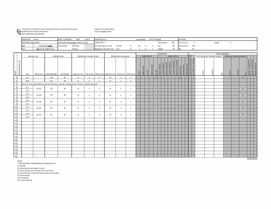
International Institute for Geo‐Information Science and Earth Observation Exposure characterizationApplied Earth Sciences Department Scan line logging sheetGeo‐engineering specialization
LOGGED BY: Andrei DATE: 13/09/2007 TIME: 13:30 h EXPOSURE No: 2 Accessibility: poor/fair/good SCANLINE
WEATHER CONDITIONS LOCATION: Montegaggio (Albiano, Italy) SLOPE FACE : 1 Dip direction 262 Scan line no. 2 Length 6
Sun: Coordinates: Northing: Size total exposure (m) l: 20.40 h: 20 d: 4 Dip 80 Dip direction O10
Rain: Easting: Mapped on this form (m) l:6.0 h: 2 d: 1 Height 20 Dip O1
DIS SPA (t/s/n) DDN (000‐360) DIP (00‐90) LEN (t/s) (m) TTN (o/r/j) BTN (o/r/j) LEN (t/s) (m) TTN (o/r/j) BTN (o/r/j) wavy
slightly wavy
curved
slightly curved
straight
rough step
ped
smoo
th stepp
ed
polishe
d step
ped
rough un
dulatin
g
smoo
th und
ulating
polishe
d un
dulatin
g
rough plan
ar
smoo
th plana
r
polishe
d plan
ar
coarse
med
ium
fine
coarse
med
ium
fine *
1 8.6 174 85 >5 o o >6 o o X X X*
2 8.86 176 84 >5 o o >6 o o
3 Becouse of the high frequency of discontinuities, spacing is obtained from (1m/no. of discontinuities)
4 8.5
5 9.5
6 9.5
7 10.5
8 10.5
9 11.5
10 11.5
11 12.7
12 12.5
13 13.4
14
15
16
17
18
19
20
21
22
23
24
25
NOTES* FINE MATERIAL CORRESPONDS TO WASHED CLAY(i): infered(j): discontinuity ends against a joint(r): discontinuity ends vanishes in the rock mass(o): discontinuity is obscured by the exposure boundary(t): total spacing(s):set spacing(n): normal spacing
cloudy/fair/bright
dry/drizzle/slight/heavy
LARGE SCALE SMALL SCALEROUGHNESS
SPACING (m) ORIENTATION PERSISTENCE ALONG STRIKE PERSISTENCE ALONG DIP
1m/16
1m/15
INFILL MATERIAL
>5
>5
>5
>5
>6 o o
>6 o
>6 o
gouge < irregularitie
s
flowing material
NUM
DISCO
NTINUITY SET
cemen
ted / cemen
ted infill
no infill / surf. Staining
gouge > irregularitie
s
non softening / sheared material softening / sheared material
>6 o o
1m/14
85
85
85
85
85
175
175
175
175
175
1m/12
1m/16
o
o
o
o
o
o
o
o
X
X
>5
o
o oo
o
>6 o X*
X*
X*
X*
X*
X
X
X
X
X
X
X
X

International Institute for Geo‐Information Science and Earth Observation Exposure characterizationApplied Earth Sciences Department Scan line logging sheetGeo‐engineering specialization
LOGGED BY: Andrei DATE: 13/09/2007 TIME: 13:30 h EXPOSURE No: 2 Accessibility: poor/fair/good SCANLINE
WEATHER CONDITIONS LOCATION: Montegaggio (Albiano, Italy) SLOPE FACE : 1 Dip direction 169 Scan line no. 3 Length 7
Sun: Coordinates: Northing: Size total exposure (m) l: 21.40 h: 20 d: 5 Dip 85 Dip direction O72
Rain: Easting: Mapped on this form (m) l:7.00 h: 2 d: 1 Height 25 Dip O4
DIS SPA (t/s/n) DDN (000‐360) DIP (00‐90) LEN (t/s) (m) TTN (o/r/j) BTN (o/r/j) LEN (t/s) (m) TTN (o/r/j) BTN (o/r/j) wavy
slightly wavy
curved
slightly curved
straight
rough step
ped
smoo
th stepp
ed
polishe
d step
ped
rough un
dulatin
g
smoo
th und
ulating
polishe
d un
dulatin
g
rough plan
ar
smoo
th plana
r
polishe
d plan
ar
coarse
med
ium
fine
coarse
med
ium
fine *
1 14.24 259 89 >5 o o >6 o o X X X*
2 14.68 252 88 >5 o o >6 o o X X X*
3 15.22 252 88 >5 o o >6 o o X X X*
4 15.94 252 85 >5 o o >6 o o X X X*
5 16.42 250 89 ‐ j o 1 j o X X X*
6 17.73 254 87 ‐ o o >6 o o X X X**
7 18.47 79 72 >3 o o >6 o o X X X*
8 19.8 254 87 >3 o o >6 o o X X X*
9
10
11
12
13
14
15
16
17
18
19
20
21
22
23
24
25
NOTES* FINE MATERIAL CORRESPONDS TO WASHED CLAY** COARSE MATERIAL CORRESPONDS TO SHEARED MATERIAL(i): infered(j): discontinuity ends against a joint(r): discontinuity ends vanishes in the rock mass(o): discontinuity is obscured by the exposure boundary(t): total spacing(s):set spacing(n): normal spacing
INFILL MATERIAL
NUM
DISCO
NTINUITY SET
cemen
ted / cemen
ted infill
no infill / surf. Staining
gouge > irregularitie
s
gouge < irregularitie
s
flowing material
non softening / sheared material softening / sheared material
cloudy/fair/bright
dry/drizzle/slight/heavy
LARGE SCALE SMALL SCALEROUGHNESS
SPACING (m) ORIENTATION PERSISTENCE ALONG STRIKE PERSISTENCE ALONG DIP
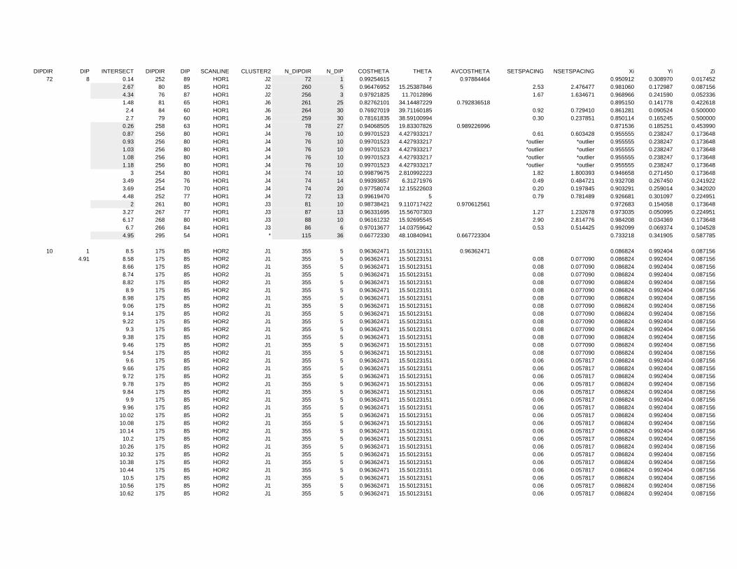
DIPDIR DIP INTERSECT DIPDIR DIP SCANLINE CLUSTER2 N_DIPDIR N_DIP COSTHETA THETA AVCOSTHETA SETSPACING NSETSPACING Xi Yi Zi72 8 0.14 252 89 HOR1 J2 72 1 0.99254615 7 0.97884464 0.950912 0.308970 0.017452
2.67 80 85 HOR1 J2 260 5 0.96476952 15.25387846 2.53 2.476477 0.981060 0.172987 0.0871564.34 76 87 HOR1 J2 256 3 0.97921825 11.7012896 1.67 1.634671 0.968966 0.241590 0.0523361.48 81 65 HOR1 J6 261 25 0.82762101 34.14487229 0.792836518 0.895150 0.141778 0.4226182.4 84 60 HOR1 J6 264 30 0.76927019 39.71160185 0.92 0.729410 0.861281 0.090524 0.5000002.7 79 60 HOR1 J6 259 30 0.78161835 38.59100994 0.30 0.237851 0.850114 0.165245 0.500000
0.26 258 63 HOR1 J4 78 27 0.94068505 19.83307826 0.989226996 0.871536 0.185251 0.4539900.87 256 80 HOR1 J4 76 10 0.99701523 4.427933217 0.61 0.603428 0.955555 0.238247 0.1736480.93 256 80 HOR1 J4 76 10 0.99701523 4.427933217 *outlier *outlier 0.955555 0.238247 0.1736481.03 256 80 HOR1 J4 76 10 0.99701523 4.427933217 *outlier *outlier 0.955555 0.238247 0.1736481.08 256 80 HOR1 J4 76 10 0.99701523 4.427933217 *outlier *outlier 0.955555 0.238247 0.1736481.18 256 80 HOR1 J4 76 10 0.99701523 4.427933217 *outlier *outlier 0.955555 0.238247 0.173648
3 254 80 HOR1 J4 74 10 0.99879675 2.810992223 1.82 1.800393 0.946658 0.271450 0.1736483.49 254 76 HOR1 J4 74 14 0.99393657 6.31271976 0.49 0.484721 0.932708 0.267450 0.2419223.69 254 70 HOR1 J4 74 20 0.97758074 12.15522603 0.20 0.197845 0.903291 0.259014 0.3420204.48 252 77 HOR1 J4 72 13 0.99619470 5 0.79 0.781489 0.926681 0.301097 0.224951
2 261 80 HOR1 J3 81 10 0.98738421 9.110717422 0.970612561 0.972683 0.154058 0.1736483.27 267 77 HOR1 J3 87 13 0.96331695 15.56707303 1.27 1.232678 0.973035 0.050995 0.2249516.17 268 80 HOR1 J3 88 10 0.96161232 15.92695545 2.90 2.814776 0.984208 0.034369 0.1736486.7 266 84 HOR1 J3 86 6 0.97013677 14.03759642 0.53 0.514425 0.992099 0.069374 0.104528
4.95 295 54 HOR1 * 115 36 0.66772330 48.10840941 0.667723304 0.733218 0.341905 0.587785
10 1 8.5 175 85 HOR2 J1 355 5 0.96362471 15.50123151 0.96362471 0.086824 0.992404 0.0871564.91 8.58 175 85 HOR2 J1 355 5 0.96362471 15.50123151 0.08 0.077090 0.086824 0.992404 0.087156
8.66 175 85 HOR2 J1 355 5 0.96362471 15.50123151 0.08 0.077090 0.086824 0.992404 0.0871568.74 175 85 HOR2 J1 355 5 0.96362471 15.50123151 0.08 0.077090 0.086824 0.992404 0.0871568.82 175 85 HOR2 J1 355 5 0.96362471 15.50123151 0.08 0.077090 0.086824 0.992404 0.0871568.9 175 85 HOR2 J1 355 5 0.96362471 15.50123151 0.08 0.077090 0.086824 0.992404 0.087156
8.98 175 85 HOR2 J1 355 5 0.96362471 15.50123151 0.08 0.077090 0.086824 0.992404 0.0871569.06 175 85 HOR2 J1 355 5 0.96362471 15.50123151 0.08 0.077090 0.086824 0.992404 0.0871569.14 175 85 HOR2 J1 355 5 0.96362471 15.50123151 0.08 0.077090 0.086824 0.992404 0.0871569.22 175 85 HOR2 J1 355 5 0.96362471 15.50123151 0.08 0.077090 0.086824 0.992404 0.0871569.3 175 85 HOR2 J1 355 5 0.96362471 15.50123151 0.08 0.077090 0.086824 0.992404 0.087156
9.38 175 85 HOR2 J1 355 5 0.96362471 15.50123151 0.08 0.077090 0.086824 0.992404 0.0871569.46 175 85 HOR2 J1 355 5 0.96362471 15.50123151 0.08 0.077090 0.086824 0.992404 0.0871569.54 175 85 HOR2 J1 355 5 0.96362471 15.50123151 0.08 0.077090 0.086824 0.992404 0.0871569.6 175 85 HOR2 J1 355 5 0.96362471 15.50123151 0.06 0.057817 0.086824 0.992404 0.087156
9.66 175 85 HOR2 J1 355 5 0.96362471 15.50123151 0.06 0.057817 0.086824 0.992404 0.0871569.72 175 85 HOR2 J1 355 5 0.96362471 15.50123151 0.06 0.057817 0.086824 0.992404 0.0871569.78 175 85 HOR2 J1 355 5 0.96362471 15.50123151 0.06 0.057817 0.086824 0.992404 0.0871569.84 175 85 HOR2 J1 355 5 0.96362471 15.50123151 0.06 0.057817 0.086824 0.992404 0.0871569.9 175 85 HOR2 J1 355 5 0.96362471 15.50123151 0.06 0.057817 0.086824 0.992404 0.087156
9.96 175 85 HOR2 J1 355 5 0.96362471 15.50123151 0.06 0.057817 0.086824 0.992404 0.08715610.02 175 85 HOR2 J1 355 5 0.96362471 15.50123151 0.06 0.057817 0.086824 0.992404 0.08715610.08 175 85 HOR2 J1 355 5 0.96362471 15.50123151 0.06 0.057817 0.086824 0.992404 0.08715610.14 175 85 HOR2 J1 355 5 0.96362471 15.50123151 0.06 0.057817 0.086824 0.992404 0.08715610.2 175 85 HOR2 J1 355 5 0.96362471 15.50123151 0.06 0.057817 0.086824 0.992404 0.087156
10.26 175 85 HOR2 J1 355 5 0.96362471 15.50123151 0.06 0.057817 0.086824 0.992404 0.08715610.32 175 85 HOR2 J1 355 5 0.96362471 15.50123151 0.06 0.057817 0.086824 0.992404 0.08715610.38 175 85 HOR2 J1 355 5 0.96362471 15.50123151 0.06 0.057817 0.086824 0.992404 0.08715610.44 175 85 HOR2 J1 355 5 0.96362471 15.50123151 0.06 0.057817 0.086824 0.992404 0.08715610.5 175 85 HOR2 J1 355 5 0.96362471 15.50123151 0.06 0.057817 0.086824 0.992404 0.087156
10.56 175 85 HOR2 J1 355 5 0.96362471 15.50123151 0.06 0.057817 0.086824 0.992404 0.08715610.62 175 85 HOR2 J1 355 5 0.96362471 15.50123151 0.06 0.057817 0.086824 0.992404 0.087156
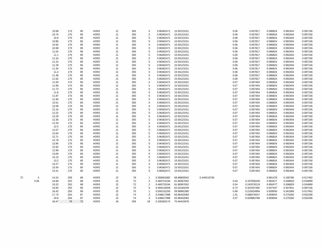
10.68 175 85 HOR2 J1 355 5 0.96362471 15.50123151 0.06 0.057817 0.086824 0.992404 0.08715610.74 175 85 HOR2 J1 355 5 0.96362471 15.50123151 0.06 0.057817 0.086824 0.992404 0.08715610.8 175 85 HOR2 J1 355 5 0.96362471 15.50123151 0.06 0.057817 0.086824 0.992404 0.087156
10.86 175 85 HOR2 J1 355 5 0.96362471 15.50123151 0.06 0.057817 0.086824 0.992404 0.08715610.92 175 85 HOR2 J1 355 5 0.96362471 15.50123151 0.06 0.057817 0.086824 0.992404 0.08715610.98 175 85 HOR2 J1 355 5 0.96362471 15.50123151 0.06 0.057817 0.086824 0.992404 0.08715611.04 175 85 HOR2 J1 355 5 0.96362471 15.50123151 0.06 0.057817 0.086824 0.992404 0.08715611.1 175 85 HOR2 J1 355 5 0.96362471 15.50123151 0.06 0.057817 0.086824 0.992404 0.087156
11.16 175 85 HOR2 J1 355 5 0.96362471 15.50123151 0.06 0.057817 0.086824 0.992404 0.08715611.22 175 85 HOR2 J1 355 5 0.96362471 15.50123151 0.06 0.057817 0.086824 0.992404 0.08715611.28 175 85 HOR2 J1 355 5 0.96362471 15.50123151 0.06 0.057817 0.086824 0.992404 0.08715611.34 175 85 HOR2 J1 355 5 0.96362471 15.50123151 0.06 0.057817 0.086824 0.992404 0.08715611.4 175 85 HOR2 J1 355 5 0.96362471 15.50123151 0.06 0.057817 0.086824 0.992404 0.087156
11.46 175 85 HOR2 J1 355 5 0.96362471 15.50123151 0.06 0.057817 0.086824 0.992404 0.08715611.52 175 85 HOR2 J1 355 5 0.96362471 15.50123151 0.06 0.057817 0.086824 0.992404 0.08715611.59 175 85 HOR2 J1 355 5 0.96362471 15.50123151 0.07 0.067454 0.086824 0.992404 0.08715611.66 175 85 HOR2 J1 355 5 0.96362471 15.50123151 0.07 0.067454 0.086824 0.992404 0.08715611.73 175 85 HOR2 J1 355 5 0.96362471 15.50123151 0.07 0.067454 0.086824 0.992404 0.08715611.8 175 85 HOR2 J1 355 5 0.96362471 15.50123151 0.07 0.067454 0.086824 0.992404 0.087156
11.87 175 85 HOR2 J1 355 5 0.96362471 15.50123151 0.07 0.067454 0.086824 0.992404 0.08715611.94 175 85 HOR2 J1 355 5 0.96362471 15.50123151 0.07 0.067454 0.086824 0.992404 0.08715612.01 175 85 HOR2 J1 355 5 0.96362471 15.50123151 0.07 0.067454 0.086824 0.992404 0.08715612.08 175 85 HOR2 J1 355 5 0.96362471 15.50123151 0.07 0.067454 0.086824 0.992404 0.08715612.15 175 85 HOR2 J1 355 5 0.96362471 15.50123151 0.07 0.067454 0.086824 0.992404 0.08715612.22 175 85 HOR2 J1 355 5 0.96362471 15.50123151 0.07 0.067454 0.086824 0.992404 0.08715612.29 175 85 HOR2 J1 355 5 0.96362471 15.50123151 0.07 0.067454 0.086824 0.992404 0.08715612.36 175 85 HOR2 J1 355 5 0.96362471 15.50123151 0.07 0.067454 0.086824 0.992404 0.08715612.43 175 85 HOR2 J1 355 5 0.96362471 15.50123151 0.07 0.067454 0.086824 0.992404 0.08715612.5 175 85 HOR2 J1 355 5 0.96362471 15.50123151 0.07 0.067454 0.086824 0.992404 0.087156
12.57 175 85 HOR2 J1 355 5 0.96362471 15.50123151 0.07 0.067454 0.086824 0.992404 0.08715612.64 175 85 HOR2 J1 355 5 0.96362471 15.50123151 0.07 0.067454 0.086824 0.992404 0.08715612.71 175 85 HOR2 J1 355 5 0.96362471 15.50123151 0.07 0.067454 0.086824 0.992404 0.08715612.78 175 85 HOR2 J1 355 5 0.96362471 15.50123151 0.07 0.067454 0.086824 0.992404 0.08715612.85 175 85 HOR2 J1 355 5 0.96362471 15.50123151 0.07 0.067454 0.086824 0.992404 0.08715612.92 175 85 HOR2 J1 355 5 0.96362471 15.50123151 0.07 0.067454 0.086824 0.992404 0.08715612.99 175 85 HOR2 J1 355 5 0.96362471 15.50123151 0.07 0.067454 0.086824 0.992404 0.08715613.06 175 85 HOR2 J1 355 5 0.96362471 15.50123151 0.07 0.067454 0.086824 0.992404 0.08715613.13 175 85 HOR2 J1 355 5 0.96362471 15.50123151 0.07 0.067454 0.086824 0.992404 0.08715613.2 175 85 HOR2 J1 355 5 0.96362471 15.50123151 0.07 0.067454 0.086824 0.992404 0.087156
13.27 175 85 HOR2 J1 355 5 0.96362471 15.50123151 0.07 0.067454 0.086824 0.992404 0.08715613.34 175 85 HOR2 J1 355 5 0.96362471 15.50123151 0.07 0.067454 0.086824 0.992404 0.08715613.41 175 85 HOR2 J1 355 5 0.96362471 15.50123151 0.07 0.067454 0.086824 0.992404 0.087156
72 4 14.24 259 89 HOR3 J2 79 1 0.358563382 68.98800542 0.449218738 0.981478 0.190780 0.0174525.56 14.68 252 88 HOR3 J2 72 2 0.469723194 61.98367002 0.44 0.197656245 0.950477 0.308829 0.034899
15.22 252 88 HOR3 J2 72 2 0.469723194 61.98367002 0.54 0.242578119 0.950477 0.308829 0.03489915.94 252 85 HOR3 J2 72 5 0.469134928 62.02184249 0.72 0.323437492 0.947437 0.307841 0.08715616.42 250 89 HOR3 J2 70 1 0.500152293 59.98992385 0.48 0.215624994 0.939550 0.341968 0.01745217.73 254 87 HOR3 J2 74 3 0.438617088 63.98432083 1.31 0.588476547 0.959944 0.275260 0.05233619.8 254 87 HOR3 J2 74 3 0.438617088 63.98432083 2.07 0.929882789 0.959944 0.275260 0.052336
18.47 79 72 HOR3 J6 259 18 0.335383174 70.40415978

Appendix 3
Appendix 3.txtParser version: 4.2.7.2Name of scan project: F:\Laser_Scan\Albiano\abiano1\Time stamp: 1189670623Time stamp: Thu Sep 13 08:03:43 2007 (UTC,1189670623)Horizontal angle: 50Vertical angle: 50Meta header version: 1Unit title: ILRIS-3DUnit serial number: SN010199Unit software version: 4.2.5Controller ID: scanner
Number of shots: 5708912Number of scan lines: 2189Number of points per line: 2608Scan task mode: scanScan task id: 0Pulse mode: Last PulseScan pattern: Step StareCalibration configuration: 0x01Shot type: Shot I3DScan start position: Lower LeftScan orientation: HorizontalScan average range(m): 46.11X spot spacing(counts/mm): 10/12.3Y spot spacing(counts/mm): 10/12.3Roi id: 32768Roi param: 0x00000030Roi start point: (-20.000000,-13.814434)Roi stop point: (19.793816,19.587627)
Applies asc correction: YesTrims shot Data: YesApplies ric correction: YesSmoothes polar shot data: NoReduces shot data: NoModel-transforms shots: YesApplies pan-tilt correction: NoRemoves outliers: NoSmoothes Cartesian shot points: NoMoves Cartesian origin: YesRange-dynamically scales intensity: Yes
Page 1

Appendix 4
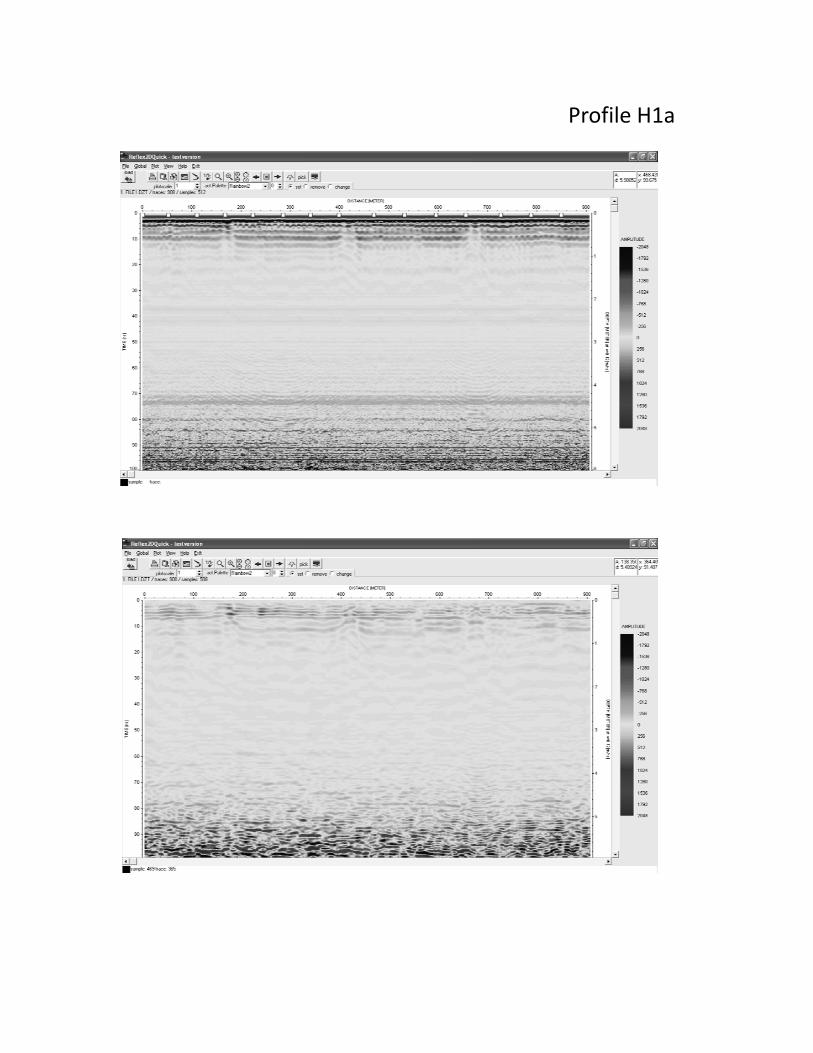
Profile H1a
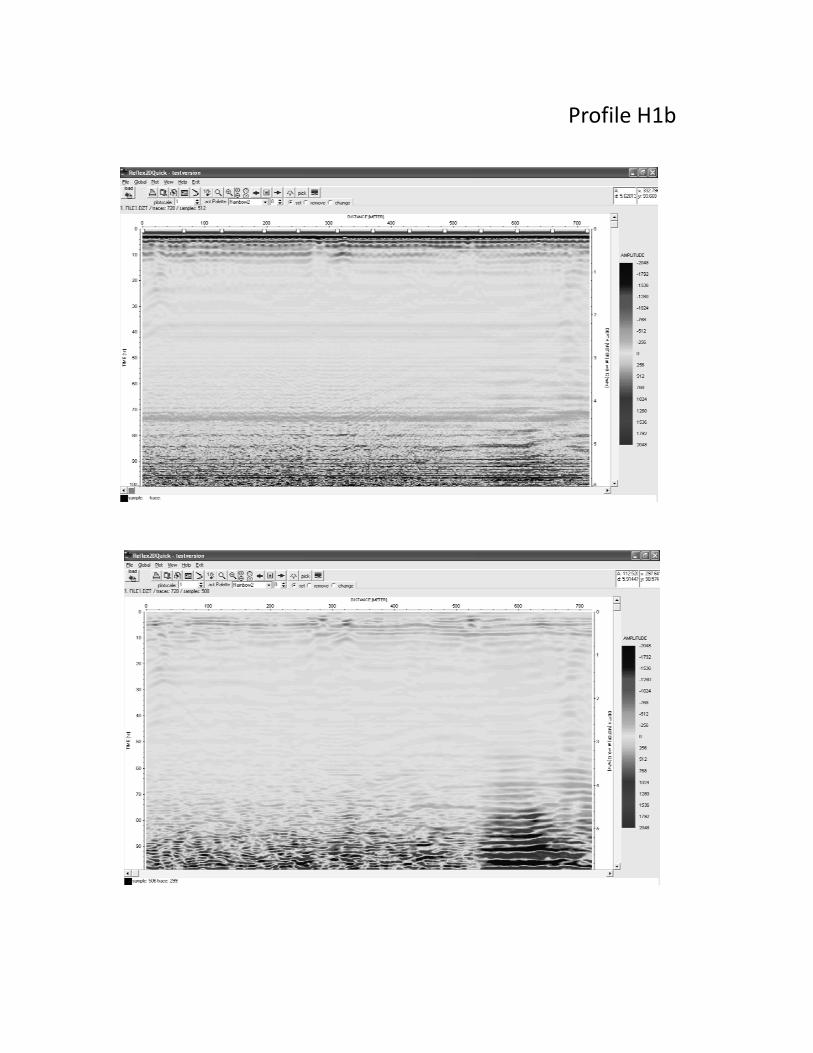
Profile H1b
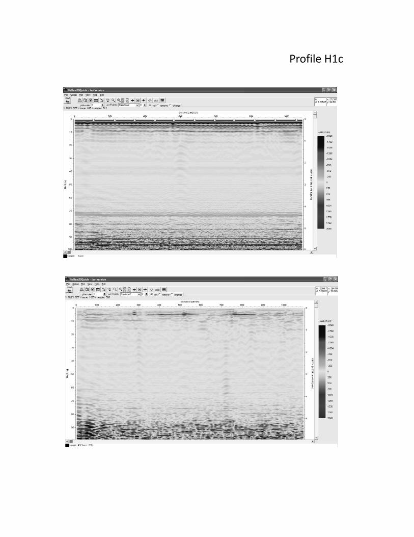
Profile H1c
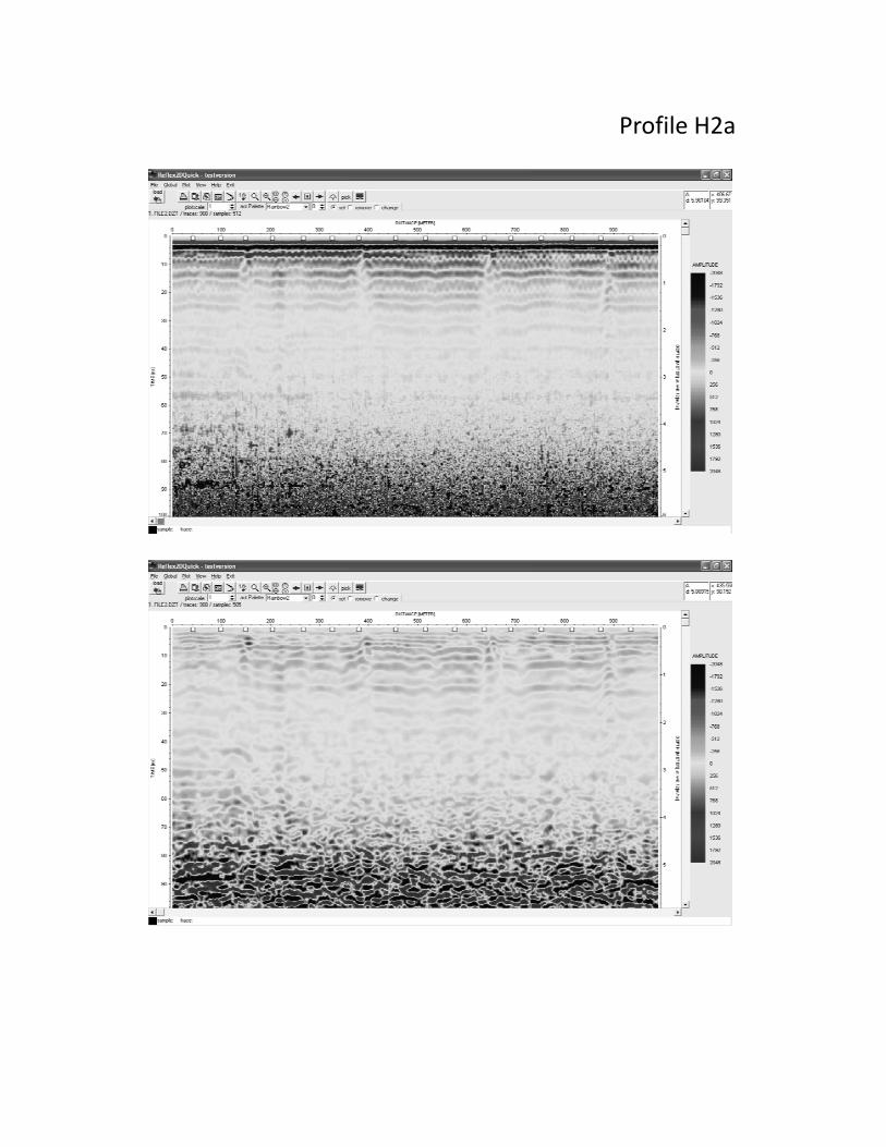
Profile H2a
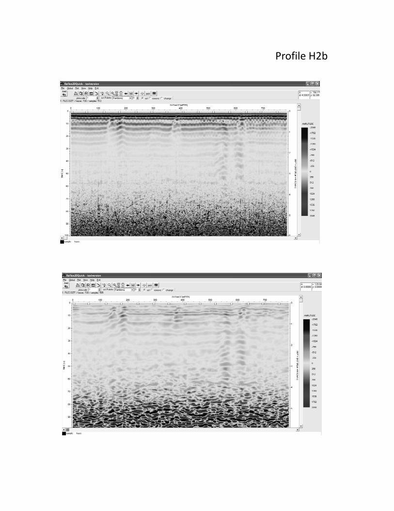
Profile H2b
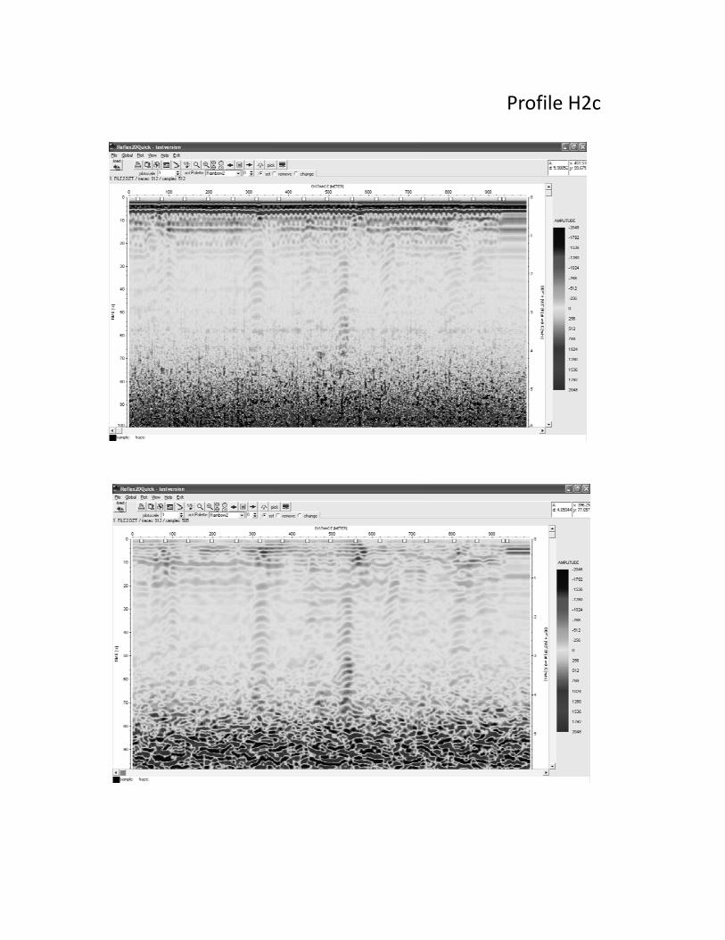
Profile H2c
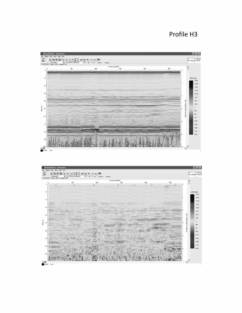
Profile H3
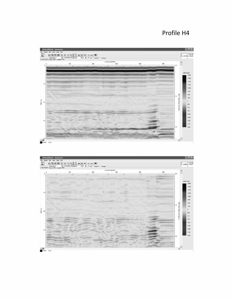
Profile H4
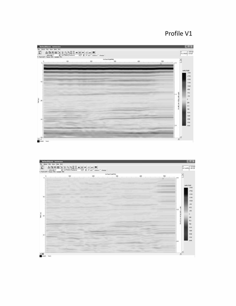
Profile V1
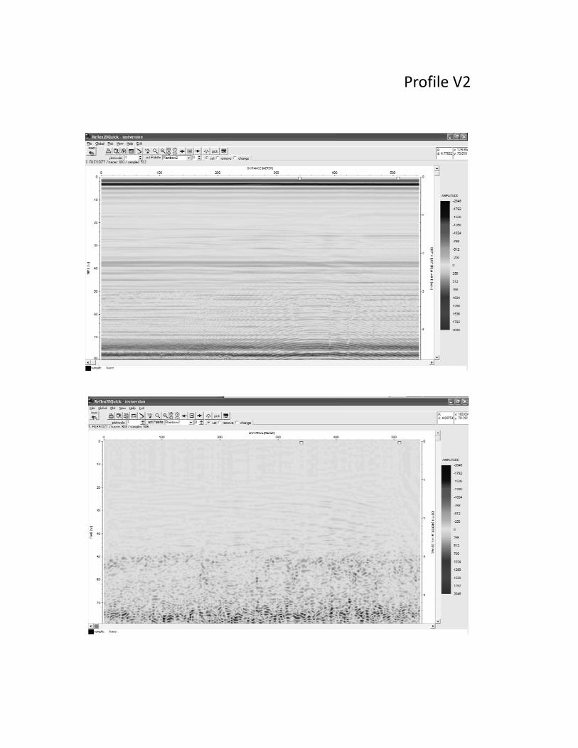
Profile V2
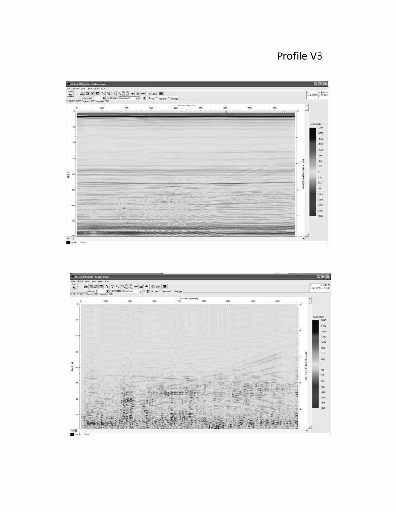
Profile V3
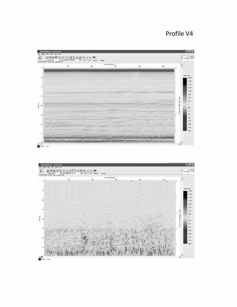
Profile V4
Recommended