Media Technology
Fachhochschule St. Pölten GmbH, Matthias Corvinus-Straße 15, 3100 St. Pölten, T: +43 (2742) 313 228, F: +43 (2742) 313 228-339, E: [email protected], I: www.fhstp.ac.at
Generative 3D computer-graphics with
POV-Ray
First Bachelor Thesis
Completed by
(Benjamin Grabner) (MT091033)
From the St. Pölten University of Applied Sciences Media Technology degree course Under the supervision of (FH-Prof. Dipl.-Ing. Markus Seidl) St. Pölten, on
June 27th, 2011 (Signature Author) (Signature Advisor)

Media Technology
2
Declaration
n I declare, that the attached research paper is my own, original work undertaken in partial fulfillment of my degree.
n I have made no use of sources, materials or assistance other than those which have been
openly and fully acknowledged in the text.
n If any part of another person’s work has been quoted, this either appears in inverted
commas or (if beyond a few lines) is indented.
n Any direct quotation or source of ideas has been identified in the text by author, date, and page number(s) immediately after such an item, and full details are provided in a reference list at the end of the text.
n I understand that any breach of the fair practice regulations may result in a mark of zero for this research paper and that it could also involve other repercussions. I understand also that too great a reliance on the work of others may lead to a low mark.
St. Pölten, on June 27th,2011 (Signature Author)

Media Technology
3
Abstract
Generative computer-graphics is a field rich in variation. It often shows complex figures with high optical
requirements. These are neither comprehensible for the viewer nor is the process of creation obvious.
Regarding this problem, the thesis aims at presenting interesting chapters of generative computer-graphics
and at outlining their backgrounds. For implementation we make use of a rendering engine named POV-Ray,
which provides a Scene Description Language to create images. This allows to completely build a 3D scene
according to own conceptions. For optimal usage and comprehension of POV-Ray, we also give an in-depth
look into the algorithm “ray tracing”, which it is based on. As the first approach to this field of knowledge we did
research on the theoretical and practical principles. Simultaneously, we develop the theoretical basics to
implement the current problem in POV-Ray. Finally, the acquired knowledge is used to create a series of
pictures. After working through this report, the reader shall be capable of realizing the introduced chapters of
generative three-dimensional computer-graphics with POV-Ray. Furthermore, it can be used as a source of
inspiration to acquire knowledge on additional generative forms and to implement such with the introduced
program.

Media Technology
4
Table of contents 1. INTRODUCTION ........................................................................................................................................................ 5 2. PRACTICAL AND THEORETICAL PRINCIPLES ............................................................................................................... 6
2.1. “GENERATIVE 3D COMPUTER-‐GRAPHICS WITH POV-‐RAY” – EXPLANATION AND BASICS ............................................................ 6 2.2. RAY-‐TRACING ............................................................................................................................................................ 10
3. GENERATIVE COMPUTER GRAPHICS ........................................................................................................................ 13 3.1 LISSAJOUS-‐FIGURES .................................................................................................................................................... 13 3.2 FRACTALS ................................................................................................................................................................. 18 3.3 THE WADA PROPERTY ................................................................................................................................................. 20
4. OWN CREATION OF GENERATIVE THREE-‐DIMENSIONAL COMPUTER-‐GRAPHICS ...................................................... 22 5. CONCLUSION .......................................................................................................................................................... 29 REFERENCES ............................................................................................................................................................... 30 APPENDIX ................................................................................................................................................................... 33

Media Technology
5
1. Introduction
The aim of this thesis is to introduce generative computer-graphics created with POV-Ray. POV-Ray is a
rendering engine that reads in text-fields containing source-code describing the scene. Then, POV-Ray uses
these statements to render a three-dimensional image. Even though we had a basic overview on the
possibilities to generate images with the Scene Description Language of POV-Ray, we had never programmed
generative graphics before. The decision of using POV-Ray is based on its feasibility to create photo-realistic
images. Thus, the algorithm this rendering engine is based on needs to be quite good and capable of
rendering beautiful images- and therefore meeting our demands concerning design. For this reason, we
managed to know how it works and how we can use its capabilities to improve the images we produce. There
is also an in-depth look on this algorithm named “ray tracing” given.
The reader isn’t required to have any previous knowledge, but it may be helpful to have written a few lines in
the source-code of this Scene Description language already. Nevertheless, the basics of POV-Ray are
described below and the range of its functions can be assumed by reading the descriptions of the practical
implementations.
At the time of this thesis’s creation in 2011, the best-selling design book on amazon.com is about generative
design, which demonstrates the current importance of the field. This is one of the main reasons for us to write
about generative three-dimensional computer-graphics. Another crucial point for choosing this topic is the
interdisciplinarity of the subject: this discipline is where programming and design meet. Another interesting
point is that ray tracing is not only used for the creation of computer graphics, but also appears in the
rendering of computer games and animated movies.
So, the research question of this thesis is:
How is it possible to implement algorithms of specific generative design chapters in a creative way?
As a first approach to this topic we used literature research to gain a basic overview of the whole range of
generative design. Then, we gradually picked out specific sections of generative design that might be
interesting and tried to implement theses algorithms with POV-Ray. The result is an extract of specific chapters
of generative art.
Section 2 contains a general introduction to the basics of POV-Ray and an in-depth look into ray-tracing, the
main algorithm which POV-Ray is based on. In Section 3 we describe the compiled parts of generative design
and give practical examples to implement them with POV-Ray. There are no significant optical requirements
needed in the realization of these sample images. Section 4 includes the practical realization of the acquired
theoretical knowledge in a creative way. A series of pictures is generated and described in this Section.
Furthermore, we focus on the graphic conversion and a common theme of these images.

Media Technology
6
2. Practical and theoretical principles
In the introductory chapter, a basic overview describes the title of this thesis and the program POV-Ray will
briefly be introduced. Furthermore, we give an in-depth examination of ray tracing, the main algorithm which is
used by POV-Ray to render images. We additionally utilize several code-snippets and images to illustrate the
given theory.
2.1. “Generative 3D computer-graphics with POV-Ray” – Explanation and Basics
Generative computer-graphics are computer graphics that base on algorithms. 3D Computer graphics - and
graphics in general - are always viewed on 2D media like displays and paper etc. Why then is it called 3D?
The answer is that the creation process of three-dimensional computer-graphics is done in a virtual three-
dimensional space. (Lauter et al. 2007, p.49) During the whole thesis we made use of a program called
Persistence of Vision Ray-Tracer (POV-Ray). POV-Ray offers possibilities to create three-dimensional, photo-
realistic images using ray-tracing. (Persistence of Vision Raytracer Pty. Ltd. 2004, p.2) Even though a lot of
experience is needed to create photo-realistic images, ray-tracing is based on the law of optics, so it
automatically allows the creation of images with tremendous light effects. (Lauter et al. 2007, p.50) A three-
dimensional scene is described in the Scene Description Language of POV-Ray and saved as a simple text-
file. POV-Ray reads in this file and generates the images from a camera, which represents the viewer.
(Persistence of Vision Raytracer Pty. Ltd. 2004, S.2) The three-dimensional scene in POV-Ray is set up in a
left-handed coordinate system, as seen in Figure 1. (Persistence of Vision Raytracer Pty. Ltd. 2008,
http://www.povray.org/documentation/view/3.6.0/15/)
figure 1: Coordinate system of POV-Ray (Persistence of Raytracer Pty. Ltd. 2008, http://www.povray.org/documentation/view/3.6.0/15)
While the positive x-axis points to the right, the positive y-axis points up and the positive z-axis into the screen.
(Persistence of Vision Raytracer Pty. Ltd. 2008, http://www.povray.org/documentation/view/3.6.0/15/) To make
it possible for POV-Ray to create a visible image, a scene’s source-code has to contain not less than one light-
source and an object as well as the description of the camera. (Lauter et al. 2007, p.49)
The source-code of the camera in the Scene Description Language of POV-Ray is: camera {
location <5,4,0>
look_at <0,0,0>
}

Media Technology
7
There are several parameters of which at least two have to be use (main parameters). The parameter
“location” refers to the position of the camera with coordinates <x,y,z>. “look_at”, as the name implies,
represents the point the camera is focusing on. (Persistence of Vision Raytracer Pty. Ltd. 2008,
http://www.povray.org/documentation/view/3.6.1/246/)
figure 2: Positioning the camera in a POV-Ray scene (Persistence of Raytracer Pty. Ltd, 2008, http://www.povray.org/documentation/view/3.6.1/246/)
As seen in Figure 2, there are a few more parameters that can be used to describe the projection on the
screen. At this point of examination, they are not necessarily needed and as a consequence, they are not
being dealt with. (Persistence of Vision Raytracer Pty. Ltd. 2008,
http://www.povray.org/documentation/view/3.6.1/246/)
After having positioned the camera, a light source is required. Otherwise, the virtual scene would be obscure
and the positioned objects invisible for the viewers. Just adding one line to the source-code does this: light_source { <0, 400, -5> color White}
The vector defines the location of the light, which is just a small point without any physical shape. (Persistence
of Vision Raytracer Pty. Ltd. 2008, http://www.povray.org/documentation/view/3.6.1/20/)
To complete a basic scene in POV-Ray, an object needs to be set up, so a simple sphere can be created by
adding these lines: sphere {
<0, 0, 0>, 1
texture {pigment {color Red}}
}
The vector defines the position of the sphere in the scene and the number after that stands fort he radius of it.
Between the „texture-command“ we colourize the sphere with „pigment { colour Red}“. (Persistence of Vision
Raytracer Pty. Ltd. 2008, http://www.povray.org/documentation/view/3.6.1/18/)
In order to use the colour-variables, it is needed to include a file in which colours are predefined at the top of
the source-code: #include "colors.inc"

Media Technology
8
(Persistence of Vision Raytracer Pty. Ltd. 2008, http://www.povray.org/documentation/view/3.6.0/16/)
There are a lot of predefined elements, especially textures allocated by POV-Ray, which are included in the
source-code the same way. Putting the source-code samples together creates the image shown in Figure 3.
The entire source-code of figure 3 and every following programmed image can be found in the appendix.
figure 3: Example of the basic functionality of POV-Ray (own rendering)
While the example in Figure 3 is fairly simple, the further scenes are more complex. Another feature of POV-
Ray is the support of combination of many simple shapes using Constructive Solid Geometry (Boolean
operations) in order to create complex objects. (Persistence of Raytracer Pty. Ltd. 2008,
http://www.povray.org/documentation/view/3.6.1/302/)
POV-Ray has four types of Constructive Solid Geometry operations:
n union (glues two objects together without removing the surface inside the union)
n intersection (builds the intersection of two objects)
n difference (builds the difference of two objects)
n merge (has the same manner as union, but eliminates the inner surface)
(Persistence of Raytracer Pty. Ltd. 2008, http://www.povray.org/documentation/view/3.6.1/303/ and
http://www.povray.org/documentation/view/3.6.1/304/ and http://www.povray.org/documentation/view/3.6.1/305/ and
http://www.povray.org/documentation/view/3.6.1/306/ and http://www.povray.org/documentation/view/3.6.1/307/)

Media Technology
9
figure 4: Example for CSG (own rendering)
Figure 4 shows an image that uses CSG, as well as a pre-defined, highly reflective chrome-textured surface,
spotlights and the default global configuration of POV-Ray. We used the texture “Chrome_Metal” for the
planes and the “egb-object”. It is located in the file “metals.inc”, included at the top of the source-code with:
#include “metals.inc”. The “egb-object” is created by using the CSG-operators “merge”, “intersection” and
“difference” and only consists of boxes and cylinders. Using additional parameters of the light source creates
the spotlights. To be more exact the parameters “spotlight”, “radius”, “point_at” and “falloff” (radius of the
umbra cone) are added. These parameters are illustrated in Figure 5. (Persistence of Raytracer Pty. Ltd. 2008,
http://www.povray.org/documentation/view/3.6.1/310/)
figure 5: Parameters of a spotlight light source (Persistence of Raytracer Pty. Ltd. 2008, http://www.povray.org/documentation/view/3.6.1/310/)

Media Technology
10
2.2. Ray-tracing
Ray tracing is a popular rendering algorithm, which is used to render three-dimensional images. The algorithm
is based on biological optics. While in reality light rays go directly or indirectly into the human’s eye, ray
tracing, as the name implies, traces the rays backwards from the ray’s origin towards the light source. In this
case, the used program POV-Ray traces back the rays from the camera positioned in the scene. So the
software has the capability to trace back all rays coming from a light source. In fact most of the rays are not
traced back, because they have no effect on the computed image. The process of rendering of the basic ray
tracing algorithm consists of two main calculations per pixel:
1. The first node is calculated. This indicates that the first point of interception from the ray with a surface
in the scene is found out.
2. To determine the colour of a point, the optical and geometric attributes of the object are used as well
as rays are sent back to each light source and previous reflections in nodes to determine the
brightness at this point.
Computing of shadow: The ray is traced back from a point to the light source. If there is an intersection the
point is in shadow. Figure 6 illustrates the basic ray-tracing algorithm. Just the colour and brightness of the first
node is calculated. There are no reflections and refractions visible.
figure 6: Basic ray-tracing algorithm illustrated with the object we created with CSG (own rendering)

Media Technology
11
3. To take reflections and transparent material in consideration, after the two main calculations are done,
ray-tracing uses the optical and geometric attributes of the object to calculate the further direction and
the intensity of colour of the computed ray. So, if the ray hits a transparent object it may splits and a
reflected and transmitted ray is generated.
For every reflected ray the steps from one to three are done again, until it reaches the maximum level of
nodes. Theoretically, an unlimited number of reflections are possible. As a consequence POV-ray uses the
maximum level of nodes is configured in the general settings and has the default value five. When the last
node is reached, the ray automatically goes back to the light source. As you can see ray-tracing is a recursive
algorithm. The brightness and colour value of the first node are used for the display pixel. So the resolution
has an effect on the number of rays that are traced back. An image with a size of 800 x 600 needs to have at
least 480000 rays to be traced back. If Anti-Aliasing is activated in POV-Ray more rays are sent out to avoid it.
(Lauter et al. 2007, p.50f; Persistence of Raytracer Pty. Ltd. 2004,
http://www.povray.org/documentation/view/3.6.1/4/ and http://povray.org/documentation/view/3.6.1/223;
Jensen und Christensen 2007, p.13ff and p.24f)
Limits of ray-tracing
Rays of light are taken in consideration only in POV-Ray, if they hit the user’s eye or like in this case the
camera. As a consequence POV-Ray cannot render two optical effects with ray-tracing only: caustics and
inter-diffuse reflections. Caustics are concentrations of lights, which occur from refracted rays from lenses and
transparent objects, displayed on other objects near the lenses for example. If a red objects is positioned in a
white room, the white room seems to have a red touch around the red object. This effect is called inter-diffuse
reflection. We can activate both effects by adding photon mapping and the radiosity algorithm to ray-tracing to
be able to show caustics and inter-diffuse reflections. (Lauter et al. 2007, p.55) To activate the possibility to
show inter-diffuse reflections in a POV-Ray scene, we have to include the file #include "rad_def.inc" and
activate the radiosity in the global settings of POV-Ray with the following lines: global_settings { radiosity { Rad_Settings(Radiosity_Normal,off,off) } max_trace_level 256 ambient_light rgb <1,1,1> }
Radiosity is not only used for inter-diffuse reflections, we can use it whenever we want to achieve a realistic
look of indirect light and as a consequence always when we want that rays of light reflected from objects have
an effect on the colour of other objects. (Persistence of Raytracer Pty. Ltd. 2004, p.2; n.a. 2010
http://wiki.povray.org/content/HowTo:Use_radiosity)
To create an optimal image, the depth of traced rays is set to the maximum with “max_trace_level”. Using
radiosity and the high depth of traced rays generates the image, showing the CSG-operations, in Figure 7. If
we add the parameter “ambient” to objects in the SDL of POV-Ray, it is also possible to create inter-diffuse
reflections, but they don’t seem very realistic, so we use the method described above. (Persistence of
Raytracer Pty. Ltd. 2008, http://www.povray.org/documentation/view/3.6.1/268/)

Media Technology
12
figure 7: CSG example rendered with maximum depth of traced rays and radiance (own rendering)
The improvement of quality in Figure 7 compared to Figure 4 is easily visible.
Rendering the image shown in Figure 7 on a dual-core AMD processor with 2.4GHz and 2GB of RAM took 1
minute and 44 seconds, which points out the enormous computing power needed by ray-tracing and the
radiosity feature.
There is also the possibility to add caustics – concentration of light - in a POV-Ray scene by activating the so-
called Photon Mapping algorithm. While this is not relevant for this thesis, we only want to point out this
possibility and don’t show the exact way to implement it.
Relevance of ray tracing
POV-Ray uses ray tracing to render images, which is one of the main reasons for it being used in the thesis.
As mentioned above, it requires great computing power to render images - and even greater computing power
to render images in real-time.
Nevertheless, it supposedly will be more often implemented in computer games in future. During CeBIT 2011,
Daniel Pohl, an Intel scientist, introduced the game “Wolfenstein” rendered in real-time, using a client-server-
setup. The game’s graphics have been rendered on four servers with integrated Knight-Ferry-Cards (32 x86-
Cores with 1.2 GHz and 4-time hyper-threading) and then sent to a client over network. Because of the
computing power needed, ray tracing’s use in computer games is expected in three to five years at the
earliest. Hybrid computer games using both ray tracing and rasterizing are likely to be published first. (Hegel
2011, http://www.hardware-infos.com/news.php?news=3867)
Media Technology
13
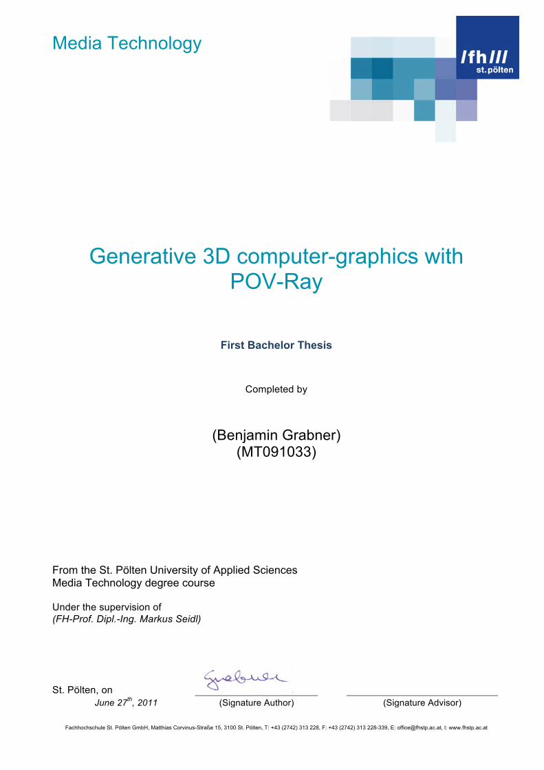
Furthermore, ray tracing is also applied in animated movies. Initially used by Pixar in the movie “A bug’s life” in
1998 to add reflections and refractions in glass bottles, ray tracing can also be found in current movies like
2007’s “Ratatouille”. For instance, Figure 8 shows ray-traced wine glassed in the movie “Ratatouille”. (Jensen
und Christensen 2007, p.46 and p.47)
figure 8: B Ray-traced glasses in the movie “Ratatouille” (Jensen und Christensen 2007, p.48 - © 2007 ®Disney/™Pixar)
3. Generative computer graphics
The following chapter includes an overview of possibilities to create generative computer graphics. A definition
and an example of fractals will be given, as well as Lissajous-figures will be described. The Pythagoreans
didn't regard mathematics as a tool. Because of the mystique quality and the immateriality of numbers, they
consider them as a manifestation of god in our world. (Bohnacker et al. 2010, p.40). In the further
considerations about generative design, this thought will be considered by using specific mathematic
algorithms to render 3D images.
3.1 Lissajous-figures
A class of variable, formed curves result from an overlay of various sine waves. These types of forms are
named after their inventor Jules Antoine Lissajous – the Lissajous-Figures. In the following paragraphs there
will be an in-depth look into the basics of harmonic waves to more complex 3D Lissajous-figures. (Bohnacker
et al. 2010, p.348) Every Lissajous-figure is based on a harmonic wave. The mathematical approach to a
harmonic wave is easy. It is characterized by sinusoids. (Bohnacker et al. 2010, p.349) First of all, a specific
point on a circular path is assumed. Then, the vertical distance from that point to the horizontal axis is
measured. Now drawing the length – the sine of the angle - of that distance in a coordinate system based on
the horizontal axis creates the sinusoid by doing that for every angle.

Media Technology
14
figure 9: Description of the construction of a sinusoid (c.f. Bohnacker et al. 2010, p.350)
The horizontal moving of the sinusoid is called phase shift. In general, the dissent angle is called phi.
(Bohnacker et al. 2010, p.349) The following lines define the source-code of Figure 10 of the sinusoid,
programmed in POV-Ray:
#declare freq=1; #declare r=0; #while (r<=2) sphere{<r,sin(r*freq*pi),0>,.01 pigment{color Black}} #declare r=r+0.001; #end
figure 10: Sinusoid rendered in POV-Ray (own rendering)
The variable “freq” defines the frequency. The angular position in radians result from the variable “R” multiplied
with “pi”. For every point on the sinusoid, a little sphere is rendered in the three-dimensional space of POV-
Ray. Switching from harmonic waves to Lissajous-figures is trivial. Just a calculation of two harmonic waves is
needed. One of them defines the x-coordinate, the other defines the y-coordinate of one point one a wave.
(Bohnacker et al. 2010, p.350) Like in the example above, we implemented these points by spheres in POV-
Ray. Figure 11 shows different Lissajous-figures rendered in POV-Ray. The frequency of the waves defining
the x-coordinate and y-coordinate, as well as the phase shift are written below the images.

Media Technology
15
figure 11: Series of Lissajous-figures (c.f. Bohnacker et al. 2010, p.352)
The following lines of source-code define the form in the right bottom corner of Figure XIII. #declare freqX=13; #declare freqY=23; #declare r=0; #while (r<=2) #declare sinx=sin(r*pi*freqX+radians(75)); #declare siny=sin(r*freqY*pi); sphere{<sinx,siny,0>,.01 pigment{color Black}} #declare r=r+0.0001; #end As written above the source-code does not differ fundamentally according to the source-code of the sinusoid.
The variables “sinx” and “siny” define the waves, which determine the current point visualized by the sphere.
Above, the frequencies for these waves are defined by the variables “freqX” and “freqY”. To add more complexity and variation to Lissajous-figures, we add modulated waves to determine the point of
a calculated wave. To implement this feature in a program, two curves need to be multiplied. Modulation is used in telecommunications to transmit pieces of information through waves in signals. For
example, radio programs transmit music and speech. These information need to be combined with a carrier
signal. As a result, the amplitude of the carrier signal gets modulated, and therefore it is also called amplitude
modulation. (Bohnacker et al. 2010, p.353) Figure 12 shows a modulated signal (blue), its carrier signal (red)
and the information signal (black) rendered in POV-Ray.

Media Technology
16
figure 12: Modulated signal (c.f. Bohnacker et al. 2010, p.353)
Now building Lissajous-figures with modulated waves has a result as shown in Figure 13.
figure 13: Lissajous-figure with modulated waves (own rendering)
Figure 13 consists of two modulated waves, created by four signals with the frequencies 4,6,8 and 10. One
wave has a phase shift of 90°. In the middle of Figure 13 one can suppose to see an abstract guy sitting cross-
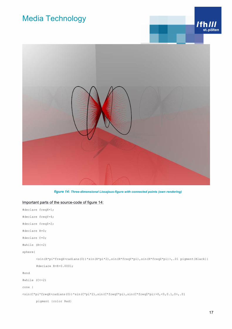
legged. Three-dimensional Lissajous-figures To set up three-dimensional Lissajous-figures, an additional sine wave is needed describing the displacement
of the spheres on the z-axis. This method offers new possibilities like connecting the original coordinates with
the following computed points in the wave with geometric forms to generate complex objects. (Bohnacker et al.
2010, p.354) These types of figures are illustrated below in Figure 14.
Media Technology
17
figure 14: Three-dimensional Lissajous-figure with connected points (own rendering)
Important parts of the source-code of figure 14: #declare freqX=1; #declare freqY=4; #declare freqZ=2; #declare R=0; #declare C=0; #while (R<=2)
sphere{
<sin(R*pi*freqX+radians(0))*sin(R*pi*2),sin(R*freqY*pi),sin(R*freqZ*pi)>,.01 pigment{Black}} #declare R=R+0.0001; #end #while (C<=2) cone { <sin(C*pi*freqX+radians(0))*sin(C*pi*2),sin(C*freqY*pi),sin(C*freqZ*pi)>0,<0,0.1,0>,.01 pigment {color Red}

Media Technology
18
} #declare C=C+0.01; #end The first while-loop generates the waves by drawing connected spheres in the three-dimensional space. An
additional sine wave is added to compute the waves in the 3D room. The frequencies used for the x-, y- and z-
axis of the waves are 1,4 and 2. The second while-loop draws cones from the centre of the Lissajous-figure to
the calculated points of the wave. It is not as often iterated as the while-loop generating the spheres, because
there is no need for a connection between the cones. In fact, we endeavour the contrary: too many cones
would reduce the aesthetic quality of this image. 3.2 Fractals
The term "fractal" is based on the Latin word "fractus", which means "scattered" and was initially defined by
Benoit Mandelbrot. (Mandelbrot 1991, p.16) The self-similarity of parts of fractals according to the whole
object, which is a main characteristic of fractals, influenced the naming. This correlation is called scale
invariance, which means that the object seems to have the shape of the whole object at a specific scale factor.
(Steidelmüller 2005, p.5) The term "dimension" is not clearly determined. There are many mathematical
approaches, that go hand in hand, but they are not identical. Mandelbrot defines it as a number of expansions.
(Mandelbrot 1991, p.26)
Consider a line, if we subdivide the line in half then it takes two bits to recreate the original line. If we
subdivide the line into 4 pieces it takes 4 of them to cover the line. We can write this generally, if we
have a line segment of length "s' then the number of segments that will cover the original line is given
by N(s) = (1/s)1. (Bourke 2003, http://paulbourke.net/fractals/fracdim/)
If a square is divided into smaller squares each with a half of the original side length, it takes four pieces to
create the original square. Repeating this step using the four originated squares, it takes sixteen squares –
now having a quarter of the original side length - to form the original square. As written above this algorithm
can be described by the formula: N(s) = (1/s) 2. The formula for the same process dividing a cube is: N(s) =
(1/s)3. (Bourke 2003, http://paulbourke.net/fractals/fracdim/)
Example:
A square has a side length of 1cm. It is divided two times, so the current length of a square is 0.25cm.
Substituting this number into this formula (1/0.25) results 16 – the number of parts, that are needed to recreate
the length of the original object. "The exponents 1, 2, and 3 in the above examples are fundamental to our
concept of the dimension involved." The formula can be generalised to N(s) = (1/s)D where D is the dimension.
To calculate the dimension, a transformation of the formula by taking logarithms of both sides is needed -

Media Technology
19
log(N(s)) = D*log(1/s). If the result of calculating D is not an integer, then this is a fractal dimension. (Bourke.
2003, http://paulbourke.net/fractals/fracdim/)
So, another main definition point of fractals is the fractal dimension, which is not an integer dimension
(Hausdorff-Besicovitch-dimensions). As a consequence they go beyond the topological dimensions. (
Mandelbrot 1991, p.27) Topological dimensions (DT) are integer dimensions, that go hand in hand with human
intuition of the real world. (Steidelmüller 2005, S.8) For most of the fractals D>DT is applied, while DT is an
integer value and D is not an integer value. (Mandelbrot 1991, p.27)
Sierpinski gasket
The dimension of the Sierpinski gasket is log(3)/log(2). The rounded result of this calculation is 1.5849625. So
its dimension lies between a line and a plane. The geometric construction of this object starts with a triangle.
For the first iteration step a horizontally mirrored triangle with half of the height of the original triangle is cut out
in the middle of the form. Like shown bellow in Figure 15, The same thing is done with the recently generated
triangles, resulting from the cut-off of the mirrored half-height triangle. Theoretically the iterations last until
infinity. The speciality about the Sierpinski gasket is the perfect self-similarity. (Bourke 1993,
http://paulbourke.net/fractals/gasket/)
figure 15: First iteration step of the Sierpinski gasket (Kost 2006, http://povray.tashcorp.net/tutorials/qd_sierpinski/)
Three-dimensional Sierpinski gasket
The original form is displaced by a four-sided pyramid to build a 3D Sierpinski gasket. The dimension D of this
fractal is the result of log(5) / log(2) = 2.321928095. (Bourke 1993, http://paulbourke.net/fractals/gasket/) For
every iteration step, the original form is displaced by 5 scaled versions, leaving a gap in the middle. (Kost
2006, http://povray.tashcorp.net/tutorials/qd_sierpinski/) There are no pre-defined forms of pyramids available
in POV-Ray. Thus, it is needed to construct a pyramid by using Constructive Solid Geometry. The source-code
of a pyramid written in den Scene Description Language of POV-Ray, looks as follows:

Media Technology
20
difference{
box {< 1,1,1>, <-1,0,-1>}
plane { x-y, -sqrt(2)/2 }
plane { -x-y, -sqrt(2)/2 }
plane { z-y, -sqrt(2)/2 }
plane { -z-y, -sqrt(2)/2 }
}
(Kost 2006, http://povray.tashcorp.net/tutorials/qd_sierpinski/)
Recursive programming is needed to build the iteration steps of the three-dimensional Sierpinski gasket. POV-
Ray provides the #macro-command to enable recursions in its Scene Description Language. (Persistence of
Vision Raytracer Pty. Lpt. 2008, http://www.povray.org/documentation/view/3.6.1/243/) In POV-Ray, the
keywords x, y and z represent the vectors <1,0,0>, <0,1,0>, <0,0,1>. (Lohmüller 2011, http://www.f-
lohmueller.de/pov_tut/calc/math_600d.htm) As parameters of the macro, we use the recursion depth, the edge
length and the vectors of the pyramid base. For every step, the current pyramid is split into five smaller
pyramids with half the edge length of the previous pyramid. This is for us aiming at leaving out the gap in the
middle. So, we place four pyramids and then one on top of them. (Kost 2006,
http://povray.tashcorp.net/tutorials/qd_sierpinski/) The splitting is done until the recursion ends. Then, the
pyramids get rendered, which is done for every 5 pyramids in the first iteration, and so on. So, the macro calls
itself for five times. The source-code for the recursion is shown below:
union {
sierpinski(s/2, center + s/2*y, recStep- 1)
sierpinski(s/2, center - s/2*(x+z), recStep - 1)
sierpinski (s/2, center - s/2*(x-z), recStep - 1)
sierpinski (s/2, center - s/2*(-x+z), recStep - 1)
sierpinski (s/2, center - s/2*(-x-z), recStep - 1)
}
(Kost 2006, http://povray.tashcorp.net/tutorials/qd_sierpinski/)
When the recursion comes to an end, the pyramid gets rendered as written above and scaled with the current
edge length and positioned to the current base centre. (Kost 2006,
http://povray.tashcorp.net/tutorials/qd_sierpinski/)
3.3 The Wada property
Wada was a Japanese mathematician. One of his students named that property in his honour. When three
basins of attractions are convoluted in a way that every point of a basin is also on the boundary of all other
basins, this state is called Wada property. On these boundaries, fractal structures do appear. (Bourke 1998,
http://paulbourke.net/fractals/wada/) Basins of attractions is a method defined by Newton used to find the roots
of a complex equitation, but it also implies the consideration about which initial guesses lead to which roots.
(Frame et al. 2011,

Media Technology
21
http://classes.yale.edu/Fractals/Mandelset/ComplexNewton/NewtonBasins/NewtonBasins.html) For a given
root, the collection of all such guesses is called the basin of attraction of that root. “ (Frame et al. 2011,
“http://classes.yale.edu/Fractals/Mandelset/ComplexNewton/ComplexNewton.html) The optical realization of
the Wada property is possible by positioning four highly reflective spheres with identical radius in a pyramid
formation. The crucial thing is that each sphere has to touch each other sphere. As a consequence, multiple
reflections of each sphere appear on every sphere and fractals do occur. (Bourke 1998,
http://paulbourke.net/fractals/wada/)
So as the first step we position three spheres in the x-z-layer of POV-Ray. The centres of the spheres are
positioned in the surrounding of a virtual circle in the same space. To simplify matters, the first sphere is
positioned on the z-axis, so the coordinate-number of z is the radius of the virtual circle and x is 0. In all further
considerations, y is assumed 0 because the three spheres are positioned in a plane. So, the centre of the first
sphere is C1<0,0,4>, if the virtual sphere is positioned in <0,0,0> and its radius is 4. Figure 16 below helps to
visualize the further considerations. Now, deriving the centre of the two other spheres from these assumptions
implies the following calculations.
figure 16: Construction of an optical Wada basing (c.f. Asti 2009, http://asti.vistecprivat.de/mathematik/frakt_pro_wada.html)
The centres of the spheres are situated on the circumference of the virtual sphere with the radius s. So, the
Pythagorean theorem can be used to calculate the two missing centres. In this case, the variables of
Pythagorean theorem are s2 = x12+y12. However, first we calculate the line z1 by applying the sine on the
angle between x1 and s. The angle has 30° because the three points around the circle are equally spaced
around it. As a consequence, there is a gap of 120° between them. Between the distance from 0 to M3 and x1,
the angle contains 90°. Subtracting this angle from the gap’s angle of 120° results in an angle of 30° between
x1 and z1. The sine of 30 is 0.5.
Media Technology
22
Now putting the assumed length of s, which is 4, and the calculated distance of z1 in the Pythagorean theorem
results in the following formula for x1 = SQRT(42-0.52). “x1” is the radius of the circle. In order to finish this
calculation, we proceeded with the assumption of s=4, making it fairly easy. Programming the optical Wada
lakes might include a distinction of s or an opportunity to declare “s” in an input-field. So the conditional
equation is needed.
1. x1 = r
2. s2 = r2 + z12
3. sin(30) = 1/2 = z1/s => z1=s/2
3. in 2.: s2 = r2 + (s/2)2 => r2=3/4*s2 => r = s* SQRT(3/4)
The resulting centre points are M1 <s*SQRT(3/4) , 0, s/2> and M2 <-s*SQRT(3/4),0,s/2). M3 stays the same
as mentioned above <0,0,-s>. With the acquired knowledge we can easily program the position of the three
spheres in the horizontal plane of POV-Ray either by using the macro-operation and using the conditional
equation or just by pre-defining the length of s.
If the camera is positioned on the y-axis and looks at the positive direction, the fourth sphere has to be
positioned on <0,2*r*SQRT(2/3),0>.
If we now position these spheres with the described vectors in a POV-Ray-scene and apply highly reflective
textures to them, the multitude reflections of each of the spheres will create fractals. (c.f. Asti 2008,
http://asti.vistecprivat.de/mathematik/frakt_pro_wada.html)
4. Own creation of generative three-dimensional computer-graphics
In the final chapter, we apply the acquired knowledge by creating high-resolution computer-graphics. The aim
is to use the given theory above in a creative way and to create three-dimensional computer-graphics with high
optical requirements. To be more detailed, we will create a three-dimensional Lissajous-figure, a three-
dimensional Sierpinski-gasket and optical basin boundaries packed in an optically attractive environment.
Lissajous-figures
In this picture we used the three-dimensional Lissajous-figure programmed in Section 3 and placed it in a
hollow box with highly reflective interior surfaces. This condition theoretically creates infinity because two
mirrors directly positioned vis-à-vis create this effect. So, in actuality there is just one Lissajous-figure placed in
this box. The infinity exists only theoretically because the number of reflections is limited by POV-Ray. The
maximum count of reflections available in POV-Ray is 256. We configured 50 reflections in the source-code of
this image, leading to a rendering-time of about fifteen minutes on a computer with dual-core processor and
two gigabyte of RAM. The main reason for us to utilize the infinity-effect in this calculated image is the fact that
fractals with we deal with in this thesis also theoretically generate infinity. We wanted to use this fact as the
common theme in our series of pictures. To make the objects visible, we had to place the camera and the
light-source, which is white, in the box mentioned above. In the appendix, the reader can find the whole
source-code of this image.

Media Technology
23
figure 17: 3D Lissajous-figure in mirrored box (own rendering)
Sierpinski-gasket
Creating this image, we also utilized the approaches of Section 3 about the creation of the three-dimensional
Sierpinski gasket. So CSG and a recursive macro were made use of. The Sierpinsk-gasket was created by
using five iterations and is now placed on a plane with a chrome-metal texture causing the reflections. As a
background we put a starry sky in this picture, available in POV-Ray 3.7beta as a source-code sample.
The result is a scene, which reminds of a Star Wars spaceship. As already mentioned next to the first picture
in Section 4, the source-code of this scene is also available in the appendix.

Media Technology
24
figure 18: 3D Sierpinski-gasket in a starry night (own rendering)
Basins of Wada
Just as above, we used the theory of Section 3 to create the following images. In the creation process, special
attention was dedicated to the background, the colours of the objects, the light-sources or the parameters of
the camera. The four spheres were positioned in the scene exactly as described above and a highly reflective
texture was applied to them. As a consequence, the reader can see fractals occur in the surfaces of these
spheres created by the multitude reflections.
In the first image below we set the colours for the spheres as blue, red, green and yellow and applied a black
background to the scene. The background shines through the gaps between the spheres. Thus, fractals in
rainbow colours appear on the finishes of the spheres.

Media Technology
25
figure 19: Optical basins of Wada in rainbow colours (own rendering)
For the next images, we rotated the camera, set a sky-sphere, which is available in POV-Ray 3.7beta for
integration into the scene and which also has an effect on the displayed colour of the reflections. Furthermore,
we activated the radiosity in the global settings of the POV-Ray scene in the second image following to cause
the colours of the objects to have an impact on each other.

Media Technology
26
figure 20: Optical basins of Wada with rotated camera and a sky sphere background (own rendering)
Media Technology
27
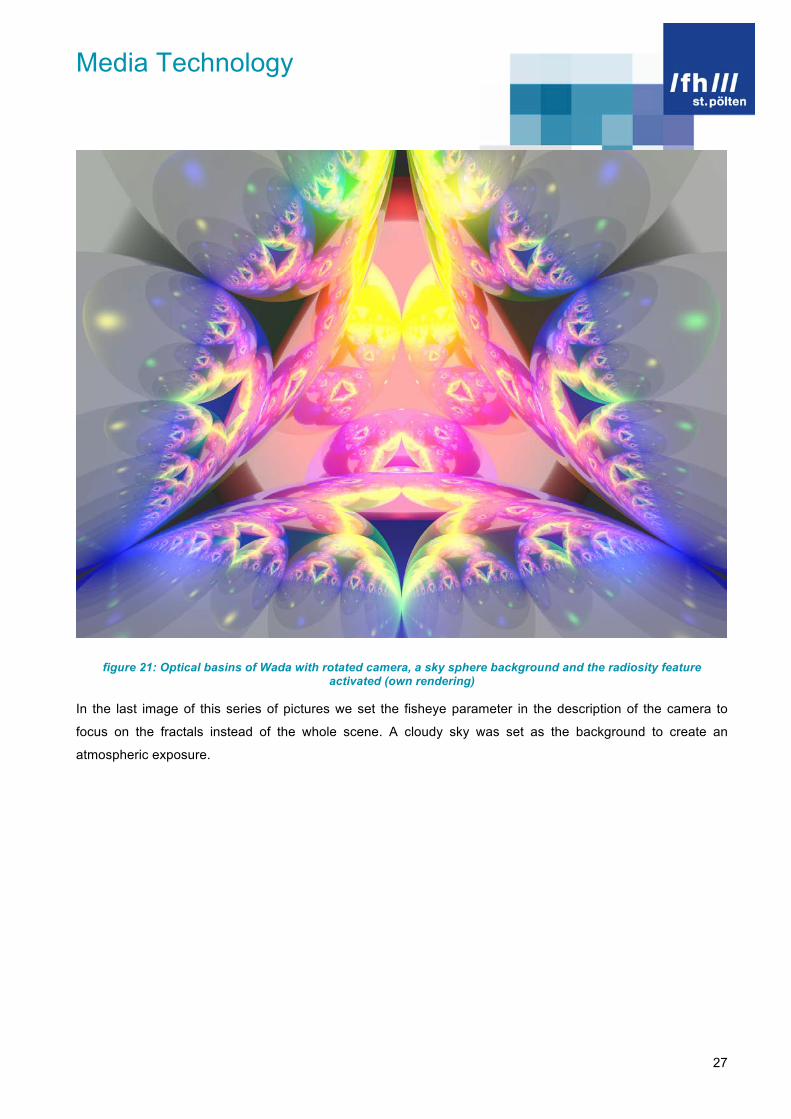
figure 21: Optical basins of Wada with rotated camera, a sky sphere background and the radiosity feature activated (own rendering)
In the last image of this series of pictures we set the fisheye parameter in the description of the camera to
focus on the fractals instead of the whole scene. A cloudy sky was set as the background to create an
atmospheric exposure.

Media Technology
28
figure 22: Optical basins of Wada viewed through a fisheye camera (own rendering)
To finish this chapter, we want to present a special picture. It contains the optical basin boundaries visible
through a camera with a bumpy lens. The following line of source-code is an example of the parameter, which
is applied to the camera-command of POV-Ray and which we made use of to render the image in Figure 23: normal {bumps 0.5 scale 0.1 translate <-50,40,0>}
(Persistence of Vision Raytracer Pty. Ltd. 2008, http://www.povray.org/documentation/view/3.6.1/249/)
Even if this image deviates from the common theme of this series of pictures, we wanted to integrate it,
because it was our desire to point out this interesting effects created by the parameter of the camera.

Media Technology
29
figure 23: Distorted basins of Wada (own rendering)
5. Conclusion
How is it possible to implement algorithms of specific generative design chapters in a creative way? This
research question is finally answered in Section 4 above. We used the theory of specific chapters of
generative design worked out in Section 3 and created new images with POV-Ray. Although our computers
were not fast and we consequently had to accept long rendering times, we created a couple of interesting
images. So, we recommend to the reader to use fast computers to generate complex images with POV-Ray.
Nevertheless, POV-Ray is ideal to create generative images and especially experimenting with specific
commands can lead to interesting pictures.

Media Technology
30
References
Asti (2009). Programmierung von Wada-Fraktalen [http://asti.vistecprivat.de/mathematik/frakt_pro_wada.html] (access on 17 May 2011) Bohnacker, H. / Groß, B. / Laub, J. / Lazzeroni, C. (Hg.) (2010). Generative Gestaltung. Entwerfen Programmieren Visualisieren.2.Auflage. Mainz: Hermann Schmidt Bourke, P. (2003). Fractal Dimension Calculator [http://paulbourke.net/fractals/fracdim/] (accessed on 26 May 2011) Bourke, P. (1993). Sierpinski Gasket [http://paulbourke.net/fractals/gasket/] (accessed on 04 May 2011) Bourke, P. (1998). Wada basins or Rendering chaotic scattering [http://paulbourke.net/fractals/wada/] (accessed on 04 May 2011) Frame, M. / Mandelbrot, B. / Neger, N. (2011). Newton’s Method Basins of Attraction [http://classes.yale.edu/Fractals/Mandelset/ComplexNewton/NewtonBasins/NewtonBasins.html] (accessed on 02 June 2011) Frame, M. / Mandelbrot, B. / Neger, N. (2011). Complex Newton’s Method [http://classes.yale.edu/Fractals/Mandelset/ComplexNewton/ComplexNewton.html] (accessed on 02 June 2011) Hegel, W. (2011) CeBIT: Spiele in Zukunft mit Raytracing? [http://www.hardware-infos.com/news.php?news=3867] (accessed on 23 March 2011) Jensen, H. W./ Christensen, P. (2007). High quality rendering using ray tracing and photon mapping. Paper at ACM SIGGRAPH New York [https://acm.fhstp.ac.at/ft_gateway.cfm?id=1281593&type=pdf&coll=DL&dl=ACM&CFID=28860461&CFTOKEN=24316124 ] (accessed on 26 April 2011) Kost, M. (2006). Quick and Dirty: Rendering Sierpinski’s Pyramid [http://povray.tashcorp.net/tutorials/qd_sierpinski/] (access on 30 May 2011) Lauter, M. (Hg.) / Institut für Mathematik der Universität Würzburg (Hg.) / Museum im Kulturspeicher Würzburg (Hg.) (2008). Ausgerechnet… Mathematik und Konkrete Kunst. 2.Auflage. Baunauch: Sparbuchverlage Mandelbrot, B.B.(1991). Die fraktale Geometrie der Natur. Einmalige Sonderausgabe. Basel: Birkhäuser Persistence of Vision Raytracer Pty. Ltd (2004). Introduction to POV-Ray. Williamstown [http://www.povray.org/redirect/www.povray.org/ftp/pub/povray/Official/Documentation/povdoc-3.6.1-a4-pdf.zip] (accessed on 11 April 2011) Persistence of Vision Raytracer Pty. Ltd (2010) HowTo: use radiosity
[http://wiki.povray.org/content/HowTo:Use_radiosity] (accessed on 20 May 2011)
Persistence of Vision Raytracer Pty. Ltd (2008). POV-Ray: Documentation: 1.2.11 Understanding POV-Ray’s Coordinate System [http://www.povray.org/documentation/view/3.6.0/15/] (accessed on 11 April 2011)

Media Technology
31
Persistence of Vision Raytracer Pty. Ltd (2008). POV-Ray: Documentation: 2.3.1.1 Placing the camera [http://www.povray.org/documentation/view/3.6.1/246/] (accessed on 11 April 2011) Persistence of Vision Raytracer Pty. Ltd (2008). POV-Ray: Documentation: 1.2.1.6 Defining a Light Source [http://www.povray.org/documentation/view/3.6.1/20/] (accessed on 11 April 2011) Persistence of Vision Raytracer Pty. Ltd (2008). POV-Ray: Documentation: 1.2.1.4 Describing an Object [http://www.povray.org/documentation/view/3.6.1/18/] (accessed on 11 April 2011) Persistence of Vision Raytracer Pty. Ltd (2008). POV-Ray: Documentation: 1.2.1.2 Adding Standard Include Files [http://www.povray.org/documentation/view/3.6.0/16/] (accessed on 11 April 2011) Persistence of Vision Raytracer Pty. Ltd (2008). POV-Ray: Documentation: 2.4.6 Constructive Solid Geometry [http://www.povray.org/documentation/view/3.6.1/302/] (accessed on 11 April 2011) Persistence of Vision Raytracer Pty. Ltd (2008). POV-Ray: Documentation: 2.3.3.11 Radiosity Basics [http://www.povray.org/documentation/view/3.6.1/268/] (accessed on 11 April 2011) Persistence of Vision Raytracer Pty. Ltd (2008). POV-Ray: Documentation: 1.1.2 What is Ray-Tracing? [http://www.povray.org/documentation/view/3.6.1/4/] (accessed on 11 April 2011) Persistence of Vision Raytracer Pty. Ltd (2008). POV-Ray: Documentation: 2.1.2.8 Tracing Options [http://povray.org/documentation/view/3.6.1/223] (accessed on 11 April 2011) Persistence of Vision Raytracer Pty. Ltd (2008). POV-Ray: Documentation: 2.4.7.2 Spotlights [http://www.povray.org/documentation/view/3.6.1/310/] (accessed on 11 April 2011) Persistence of Vision Raytracer Pty. Ltd (2008). POV-Ray: Documentation: 2.4.6.1 inside and Outside [http://www.povray.org/documentation/view/3.6.1/303/] (accessed on 11 April 2011) Persistence of Vision Raytracer Pty. Ltd (2008). POV-Ray: Documentation: 2.4.6.2 Union [http://www.povray.org/documentation/view/3.6.1/304/] (accessed on 11 April 2011) Persistence of Vision Raytracer Pty. Ltd (2008). POV-Ray: Documentation: 2.4.6.3 Intersection [http://www.povray.org/documentation/view/3.6.1/305/] (accessed on 11 April 2011) Persistence of Vision Raytracer Pty. Ltd (2008). POV-Ray: Documentation: 2.4.6.4 Difference [http://www.povray.org/documentation/view/3.6.1/306/] (accessed on 11 April 2011) Persistence of Vision Raytracer Pty. Ltd (2008). POV-Ray: Documentation: 2.4.6.5 Merge [http://www.povray.org/documentation/view/3.6.1/307/] (accessed on 11 April 2011) Persistence of Vision Raytracer Pty. Ltd (2008). POV-Ray: Documentation: 2.2.2.8 User defined macros [http://www.povray.org/documentation/view/3.6.1/243/| (accessed on 15 May 2011) Steidelmüller, H. (2005). Fraktale, Dimensionen und Brownsche Bewegung. [http://www-gs.informatik.tu-cottbus.de/projektstudium/vortraege/Fraktale_Dimensionen_BrownscheBewegung.pdf] (accessed on 23 May 2011)
Media Technology
32
List of figures
figure 1: Coordinate system of POV-Ray (Persistence of Raytracer Pty. Ltd. 2008, http://www.povray.org/documentation/view/3.6.0/15) ........................................................................................... 6 figure 2: Positioning the camera in a POV-Ray scene (Persistence of Raytracer Pty. Ltd, 2008, http://www.povray.org/documentation/view/3.6.1/246/) ........................................................................................ 7 figure 3: Example of the basic functionality of POV-Ray ...................................................................................... 8 figure 4: Example for CSG ................................................................................................................................... 9 figure 5: Parameters of a spotlight light source (Persistence of Raytracer Pty. Ltd. 2008, http://www.povray.org/documentation/view/3.6.1/310/) ........................................................................................ 9 figure 6: Basic ray-tracing algorithm illustrated with the object we created with CSG ........................................ 10 figure 7: CSG example rendered with maximum depth of traced rays and radiance ......................................... 12 figure 8: B Ray-traced glasses in the movie “Ratatouille” (Jensen und Christensen 2007, p.48 - © 2007 ®Disney/™Pixar) ................................................................................................................................................ 13 figure 9: Description of the construction of a sinusoid (c.f. Bohnacker et al. 2010, p.350) ................................. 14 figure 10: Sinusoid rendered in POV-Ray .......................................................................................................... 14 figure 11: Series of Lissajous-figures (c.f. Bohnacker et al. 2010, p.352) .......................................................... 15 figure 12: Modulated signal (c.f. Bohnacker et al. 2010, p.353) ......................................................................... 16 figure 13: Lissajous-figure with modulated waves .............................................................................................. 16 figure 14: Three-dimensional Lissajous-figure with connected points ................................................................ 17 figure 15: First iteration step of the Sierpinski gasket (Kost 2006, http://povray.tashcorp.net/tutorials/qd_sierpinski/) ............................................................................................. 19 figure 16: Construction of an optical Wada basing (c.f. Asti 2009, http://asti.vistecprivat.de/mathematik/frakt_pro_wada.html) .............................................................................. 21 figure 17: 3D Lissajous-figure in mirrored box .................................................................................................... 23 figure 18: 3D Sierpinski-gasket in a starry night ................................................................................................. 24 figure 19: Optical basins of Wada in rainbow colours ........................................................................................ 25 figure 20: Optical basins of Wada with rotated camera and a sky sphere background ...................................... 26 figure 21: Optical basins of Wada with rotated camera, a sky sphere background and the radiosity feature activated ............................................................................................................................................................. 27 figure 22: Optical basins of Wada viewed through a fisheye camera ................................................................. 28 figure 23: Distorted basins of Wada ................................................................................................................... 29

Media Technology
33
Appendix
Section 1 Figure 3: #include "colors.inc" camera { location <5,4,0> look_at <0,0,0> } light_source { <0,400,-5> color White } sphere { <0,0,0>, 1 texture { pigment {color Red} } } Figure 4: #include "colors.inc" #include "metals.inc" #include "textures.inc" camera { location <40, 40,-70> look_at <0,0,0> } light_source { <5, 4000, -3000> color White } light_source { <100, 15, -15> color Cyan spotlight radius 4 falloff 7 point_at <20,15,-15> } light_source { <15,100,-15> color Magenta spotlight radius 4 falloff 7 point_at <15,20,-15>

Media Technology
34
} light_source { <15,15,-100> color White spotlight radius 4 falloff 7 point_at <15,15,-20> } plane { <1,0,0>,0 texture { Chrome_Metal } } plane { <0,1,0>,0 texture{Chrome_Metal } } plane { <0,0,1>,0 texture{ Chrome_Metal } } #declare basicObject = box { <20,20,-10>, <10,10,-20> } #declare createB = merge { object {basicObject} cylinder { <19.5,20,-12.5>, <19.5,10,-12.5>,2.5 } cylinder { <19.5,20,-12.5>, <19.5,10,-12.5>,2.5 translate <0,0,-5> } } #declare neu = intersection { object{createB} cylinder { <8,15,-15>, <22,15,-15>, 6 open }

Media Technology
35
} #declare fertig = difference { object {neu} box { <22,-20,-10>, <8,10.5,-20> } box { <22,19.5,-10>, <8,30.5,-20> } box { <22,13,-8>, <12,12,-22> } box { <22,21,-22>, <9,9,-19.5> } box { <22,21,-10.5>, <9,9,-9.5> } box { <23,18,-12>, <9,16,-18> } box { <23,18,-12>, <9,16,-18> translate <0,-4,0> } box { <23,18,-18>, <9,16,-15> translate <0,-2,0> } box { <23,18,-9>, <9,16,-18> translate <0,-0.5,0> } box { <23,18,-9>, <12,16,-21> } box { <23,18,-9>, <12,16,-21> translate <0,-3.9,0>

Media Technology
36
} box { <23,18,-9>, <18,16,-21> translate <0,-2,0> } union { box { <19,21,-12>, <12,9,-14> } cylinder { <19,21,-13>, <19,9,-13>,1 } translate <0,0,0.5> } union { box { <19,21,-12>, <12,9,-14> } cylinder { <19,21,-13>, <19,9,-13>,1 } translate <0,0,-4.5> } } object { fertig texture{Chrome_Metal } } Figure 5: #include "colors.inc" #include "metals.inc" #include "textures.inc" global_settings { max_trace_level 1 } camera { location <40, 40,-60> look_at <0,0,0> } light_source { <5, 4000, -3000> color White

Media Technology
37
} light_source { <100, 15, -15> color Cyan spotlight radius 4 falloff 7 point_at <20,15,-15> } light_source { <15,100,-15> color Magenta spotlight radius 4 falloff 7 point_at <15,20,-15> } light_source { <15,15,-100> color White spotlight radius 4 falloff 7 point_at <15,15,-20> } plane {
<1,0,0>,0
texture { Chrome_Metal
}
}
plane { <0,1,0>,0 texture{Chrome_Metal } } plane { <0,0,1>,0 texture{ Chrome_Metal } } #declare basicObject = box {

Media Technology
38
<20,20,-10>, <10,10,-20> } #declare createB = merge { object {basicObject} cylinder { <19.5,20,-12.5>, <19.5,10,-12.5>,2.5 } cylinder { <19.5,20,-12.5>, <19.5,10,-12.5>,2.5 translate <0,0,-5> } } #declare neu = intersection { object{createB} cylinder { <8,15,-15>, <22,15,-15>, 6 open } } #declare fertig = difference { object {neu} box { <22,-20,-10>, <8,10.5,-20> } box { <22,19.5,-10>, <8,30.5,-20> } box { <22,13,-8>, <12,12,-22> } box { <22,21,-22>, <9,9,-19.5> } box { <22,21,-10.5>, <9,9,-9.5> } box { <23,18,-12>, <9,16,-18>

Media Technology
39
} box { <23,18,-12>, <9,16,-18> translate <0,-4,0> } box { <23,18,-18>, <9,16,-15> translate <0,-2,0> } box { <23,18,-9>, <9,16,-18> translate <0,-0.5,0> } box { <23,18,-9>, <12,16,-21> } box { <23,18,-9>, <12,16,-21> translate <0,-3.9,0> } box { <23,18,-9>, <18,16,-21> translate <0,-2,0> } union { box { <19,21,-12>, <12,9,-14> } cylinder { <19,21,-13>, <19,9,-13>,1 } translate <0,0,0.5> } union { box { <19,21,-12>, <12,9,-14> } cylinder { <19,21,-13>, <19,9,-13>,1 } translate <0,0,-4.5>

Media Technology
40
} } object { fertig texture{Chrome_Metal } } Figure 7: #include "colors.inc" #include "metals.inc" #include "textures.inc" #include "rad_def.inc" global_settings { radiosity { Rad_Settings(Radiosity_Normal,off,off) } max_trace_level 256 ambient_light rgb <1,1,1> } #default {finish{ambient 0}} camera { location <40, 40,-70> look_at <0,0,0> } light_source { <5, 4000, -3000> color White } light_source { <100, 15, -15> color Cyan spotlight radius 4 falloff 7 point_at <20,15,-15> } light_source { <15,100,-15> color Magenta spotlight radius 4 falloff 7 point_at <15,20,-15> }

Media Technology
41
light_source { <15,15,-100> color White spotlight radius 4 falloff 7 point_at <15,15,-20> } plane { <1,0,0>,0 texture { Chrome_Metal } } plane { <0,1,0>,0 texture{Chrome_Metal } } plane { <0,0,1>,0 texture{ Chrome_Metal } } #declare basicObject = box { <20,20,-10>, <10,10,-20> } #declare createB = merge { object {basicObject} cylinder { <19.5,20,-12.5>, <19.5,10,-12.5>,2.5 } cylinder { <19.5,20,-12.5>, <19.5,10,-12.5>,2.5 translate <0,0,-5> } } #declare neu = intersection { object{createB} cylinder { <8,15,-15>, <22,15,-15>, 6 open } }

Media Technology
42
#declare fertig = difference { object {neu} box { <22,-20,-10>, <8,10.5,-20> } box { <22,19.5,-10>, <8,30.5,-20> } box { <22,13,-8>, <12,12,-22> } box { <22,21,-22>, <9,9,-19.5> } box { <22,21,-10.5>, <9,9,-9.5> } box { <23,18,-12>, <9,16,-18> } box { <23,18,-12>, <9,16,-18> translate <0,-4,0> } box { <23,18,-18>, <9,16,-15> translate <0,-2,0> } box { <23,18,-9>, <9,16,-18> translate <0,-0.5,0> } box { <23,18,-9>, <12,16,-21> } box { <23,18,-9>, <12,16,-21> translate <0,-3.9,0> }

Media Technology
43
box { <23,18,-9>, <18,16,-21> translate <0,-2,0> } union { box { <19,21,-12>, <12,9,-14> } cylinder { <19,21,-13>, <19,9,-13>,1 } translate <0,0,0.5> } union { box { <19,21,-12>, <12,9,-14> } cylinder { <19,21,-13>, <19,9,-13>,1 } translate <0,0,-4.5> } } object { fertig texture{Chrome_Metal } } Section 2 Figure 10 #include "colors.inc" background{color White} light_source{<25,50,-100> color White} camera{ location <1,0,-3> look_at <1,0,0> } plane { <0,1,0>,-1.1 pigment {color Red} }

Media Technology
44
#declare Freq=1; #declare R=0; #declare Sinusoid = #while (R<=2) sphere{ <R,sin(R*Freq*pi),0>, .01 pigment{color Black} } #declare R=R+0.001; #end object { Sinusoid translate <1,0,-2> } Figure 11 1 #include "colors.inc" background{color White} light_source{<25,50,-100> color White} camera{ location <0,0,-3> look_at <0,0,0> } plane { <0,1,0>,-1.1 pigment {color Red} } #declare FreqX=1; #declare FreqY=4; #declare R=0; #while (R<=2) sphere{ <sin(R*pi*FreqX+radians(150)),sin(R*FreqY*pi),0>, .01 pigment{color Black} } #declare R=R+0.0001; #end 2 #include "colors.inc"

Media Technology
45
background{color White} light_source{<25,50,-100> color White} camera{ location <0,0,-3> look_at <0,0,0> } plane { <0,1,0>,-1.1 pigment {color Red} } #declare FreqX=6; #declare FreqY=8; #declare R=0; #while (R<=2) sphere{ <sin(R*pi*FreqX+radians(90)),sin(R*FreqY*pi),0>, .01 pigment{color Black} } #declare R=R+0.0001; #end 3 #include "colors.inc" background{color White} light_source{<25,50,-100> color White} camera{ location <0,0,-3> look_at <0,0,0> } plane { <0,1,0>,-1.1 pigment {color Red} } #declare FreqX=4; #declare FreqY=9; #declare R=0; #while (R<=2) sphere{

Media Technology
46
<sin(R*pi*FreqX+radians(195)),sin(R*FreqY*pi),0>, .01 pigment{color Black} } #declare R=R+0.0001; #end 4 #include "colors.inc" background{color White} light_source{<25,50,-100> color White} camera{ location <0,0,-3> look_at <0,0,0> } plane { <0,1,0>,-1.1 pigment {color Red} } #declare FreqX=19; #declare FreqY=9; #declare R=0; #while (R<=2) sphere{ <sin(R*pi*FreqX+radians(75)),sin(R*FreqY*pi),0>, .01 pigment{Black} } #declare R=R+0.0001; #end 5 #include "colors.inc" background{color White} light_source{<25,50,-100> color White} camera{ location <0,0,-3> look_at <0,0,0> }
Media Technology
47
plane { <0,1,0>,-1.1 pigment {color Red} } #declare FreqX=11; #declare FreqY=13; #declare R=0; #while (R<=2) sphere{ <sin(R*pi*FreqX+radians(90)),sin(R*FreqY*pi),0>, .01 pigment{color Black} } #declare R=R+0.0001; #end 6 #include "colors.inc" background{color White} light_source{<25,50,-100> color White} camera { location <0,0,-3> look_at <0,0,0> } plane { <0,1,0>,-1.1 pigment {color Red} } #declare FreqX=13; #declare FreqY=23; #declare R=0; #while (R<=2) sphere{ <sin(R*pi*FreqX+radians(75)),sin(R*FreqY*pi),0>, .01 pigment{color Black} } #declare R=R+0.0001; #end Figure 12 #include "colors.inc" background {color White} light_source{<25,50,-100> color White}

Media Technology
48
camera{ location <2,0,-4> look_at <2,0,0> } plane { <0,1,0>,-1.1 pigment {color Red} } #declare Freq=1; #declare FreqMod=5; #declare R=0; #declare T=0; #declare C=0; #while (R<=4) sphere{ <R,sin(R*Freq*pi+radians(120)),0>, .01 pigment{color Black} } #declare R=R+0.001; #end #while (T<=4) sphere{ <T,cos(T*FreqMod*pi),0>,.01 pigment{color Red} } #declare T=T+0.001; #end #while (C<=4) sphere{ <C,cos(C*FreqMod*pi)*sin(C*Freq*pi+radians(120)),0>,.01 pigment{color Blue} } #declare C=C+0.001; #end Figure 13 #include "colors.inc" background {color White} light_source{<25,50,-100> color White} camera{ location <0,0,-3> look_at <0,0,0> }

Media Technology
49
plane { <0,1,0>,-1.1 pigment {color Red} } #declare Freq=6; #declare FreqMod=8; #declare Freq2=10; #declare FreqMod2=12; #declare C=0; #while (C<=4) sphere{ <cos(C*FreqMod2*pi)*sin(C*Freq2*pi),cos(C*FreqMod*pi)*sin(C*Freq*pi+radians(90)),0>,.01 pigment{color Blue} } #declare C=C+0.0001; #end Figure 14 #include "colors.inc" #include "metals.inc" #include "textures.inc" background {color White} light_source {<5,10,-5> color White} global_settings { max_trace_level 20 } camera { location <5,1,-3> look_at <1,0,0> } plane { <1,0,0>,-4 texture {Chrome_Metal} } plane { <0,1,0>,-2 texture{Chrome_Metal pigment {color Red}} } plane { <0,0,1>,2 texture{ Chrome_Metal } }

Media Technology
50
#declare lissajousfigure = union { #declare FreqX=1; #declare FreqY=4; #declare FreqZ=2; #declare R=0; #declare C=0; #while (R<=2) sphere{ <sin(R*pi*FreqX+radians(0))*sin(R*pi*2),sin(R*FreqY*pi),sin(R*FreqZ*pi)>,.01 pigment{color Black} } #declare R=R+0.0001; #end #while (C<=2) cone { <sin(C*pi*FreqX+radians(0))*sin(C*pi*2),sin(C*FreqY*pi),sin(C*FreqZ*pi)> 0, <0,0.1,0>, .01 pigment {color Red} } #declare C=C+0.01; #end } object {lissajousfigure} Figure 17 #include "colors.inc" #include "metals.inc" #include "textures.inc" light_source{ <3,1,-2> color White shadowless } global_settings { max_trace_level 50 } camera{ location <3,1,-3> look_at <1,0,0> rotate z*20 } #declare lissajousfigure = union { #declare FreqX=1; #declare FreqY=4; #declare FreqZ=2; #declare R=0; #declare C=0; #while (R<=2) sphere{ <sin(R*pi*FreqX+radians(0))*sin(R*pi*2),sin(R*FreqY*pi),sin(R*FreqZ*pi)>,.01 } #declare R=R+0.0001;

Media Technology
51
#end #while (C<=2) cone { <sin(C*pi*FreqX+radians(0))*sin(C*pi*2),sin(C*FreqY*pi),sin(C*FreqZ*pi)> 0, <0,0.1,0>, .01 pigment {color White} } #declare C=C+0.01; #end } union { object {lissajousfigure } box { <0,-2,-4>, <4,2,0> texture {finish {reflection 1 ambient 0}} hollow } texture{Chrome_Metal pigment {color Red}} }
Figure 18 #include "functions.inc" #include "colors.inc" #include "metals.inc" #include "stars.inc" global_settings { max_trace_level 25 } camera { location <-7, 2, 6> look_at <0, 2, 0> } light_source {<0, 1, 0> color Pink} light_source {<-20, 20, 0> color White} light_source {<0, 10, 5> color Pink} sphere { <0,0,0>, 950 texture{ Starfield1 } } #macro sierpinski(s, base_center, recursion_depth) #if (recursion_depth > 0) union { sierpinski(s / 2, base_center + s/2*y, recursion_depth - 1) sierpinski(s / 2, base_center - s/2*(x+z), recursion_depth - 1) sierpinski(s / 2, base_center - s/2*(x-z), recursion_depth - 1) sierpinski(s / 2, base_center - s/2*(-x+z), recursion_depth - 1) sierpinski(s / 2, base_center - s/2*(-x-z), recursion_depth - 1) } #else difference{ box { <1,1,1>, <-1,0,-1> } plane{ x-y, -sqrt(2)/2} plane{ -x-y, -sqrt(2)/2} plane{ z-y, -sqrt(2)/2} plane{ -z-y, -sqrt(2)/2} scale s*1.5 translate base_center } #end #end object { sierpinski(4, <0, 0.5, 0>, 6) scale <0.8, 1, 0.8>

Media Technology
52
texture { T_Chrome_5E } } plane { <0,1,0>,0.5 texture { T_Chrome_5E } }
Figure 19: #include "colors.inc" #include "metals.inc" global_settings { max_trace_level 256 } camera { location <0,-1.5,0> look_at <0,0,-0.1> rotate y*180 } #declare S=2; #declare R=S*sqrt(3/4); light_source {<0, -10, 0> color White*0.6 } light_source {<0, -100, 0> color Yellow*0.6 } light_source {<0, 2*R, 10> color Pink } light_source {<-2*R, 2*R, 1> color Green} light_source {<2*R, 2*R, 1> color Red} #default{finish{F_MetalE}} union { sphere {<S*sqrt(3/4),0,S/2> R pigment{MediumForestGreen}} sphere {<-S*sqrt(3/4),0,S/2> R pigment{Yellow}} sphere {<0,0,-S> R pigment{Blue}} sphere {<0,2*R*sqrt(2/3),0> R pigment{Red}} no_shadow }
Figure 20: #include "colors.inc" #include "metals.inc" global_settings { max_trace_level 256 } camera { location <0,-1.5,0> look_at <0,0,-0.01> } plane{<0,1,0>,1 hollow texture{ pigment{ bozo turbulence 0.92 color_map { [0.00 rgb <0.25, 0.35, 1.0>*0.7] [0.50 rgb <0.25, 0.35, 1.0>*0.7] [0.70 rgb <1,1,1>] [0.85 rgb <0.25,0.25,0.25>] [1.0 rgb <0.5,0.5,0.5>]} scale<1,1,1.5>*2.5 translate< 0,0,0> } finish {ambient 1 diffuse 0} } scale 10000} fog { fog_type 2 distance 100 color White*0.5 fog_offset 0.1 fog_alt 2.0

Media Technology
53
turbulence 1.8 } #declare S=2; #declare R=S*sqrt(3/4); light_source {<0, -10, 0> color White*0.6 } light_source {<0, -100, 0> color White*0.6 } light_source {<0, 2*R, 10> color Pink } light_source {<-2*R, 2*R, 1> color Cyan} light_source {<2*R, 2*R, 1> color White} #default{finish{F_MetalE}} union { sphere {<S*sqrt(3/4),0,S/2> R pigment{Green}} sphere {<-S*sqrt(3/4),0,S/2> R pigment{Yellow}} sphere {<0,0,-S> R pigment{Blue}} sphere {<0,2*R*sqrt(2/3),0> R pigment{Red}} no_shadow }
Figure 21: #include "colors.inc" #include "metals.inc" #include "rad_def.inc" global_settings { max_trace_level 256 radiosity { Rad_Settings(Radiosity_Normal,off,off) } } camera { location <0,-1.5,0> look_at <0,0,-0.01> } plane{<0,1,0>,1 hollow texture{ pigment{ bozo turbulence 0.92 color_map { [0.00 rgb <0.25, 0.35, 1.0>*0.7] [0.50 rgb <0.25, 0.35, 1.0>*0.7] [0.70 rgb <1,1,1>] [0.85 rgb <0.25,0.25,0.25>] [1.0 rgb <0.5,0.5,0.5>]} scale<1,1,1.5>*2.5 translate< 0,0,0> } finish {ambient 1 diffuse 0} } scale 10000} fog { fog_type 2 distance 100 color White*0.5 fog_offset 0.1 fog_alt 2.0 turbulence 1.8 } #declare S=2; #declare R=S*sqrt(3/4); light_source {<0, -10, 0> color White*0.6 } light_source {<0, -100, 0> color White*0.6 } light_source {<0, 2*R, 10> color Pink } light_source {<-2*R, 2*R, 1> color Cyan} light_source {<2*R, 2*R, 1> color White} #default{finish{F_MetalE}}

Media Technology
54
union { sphere {<S*sqrt(3/4),0,S/2> R pigment{Green}} sphere {<-S*sqrt(3/4),0,S/2> R pigment{Yellow}} sphere {<0,0,-S> R pigment{Blue}} sphere {<0,2*R*sqrt(2/3),0> R pigment{Red}} no_shadow }
Figure 22: #include "colors.inc" #include "metals.inc" global_settings { max_trace_level 256 } camera { fisheye location <0,-1,0> look_at <0,0,-0.01> rotate y*60 angle 60 } plane{<0,1,0>,10 hollow texture{ pigment{ bozo turbulence 0.92 color_map { [0.00 rgb <0.25, 0.35, 1.0>*0.7] [0.50 rgb <0.25, 0.35, 1.0>*0.7] [0.70 rgb <1,1,1>] [0.85 rgb <0.25,0.25,0.25>] [1.0 rgb <0.5,0.5,0.5>]} scale<1,1,1.5>*2.5 translate< 0,0,0> } finish {ambient 1 diffuse 0} } scale 100} #declare S=2; #declare R=S*sqrt(3/4); light_source {<0, -10, 0> color White*0.6 } light_source {<0, -100, 0> color White*0.6 } light_source {<0, 2*R, 10> color Pink } light_source {<-2*R, 2*R, 1> color Cyan} light_source {<2*R, 2*R, 1> color White} #default{finish{F_MetalE}} union { sphere {<S*sqrt(3/4),0,S/2> R pigment{Green}} sphere {<-S*sqrt(3/4),0,S/2> R pigment{Yellow}} sphere {<0,0,-S> R pigment{Blue}} sphere {<0,2*R*sqrt(2/3),0> R pigment{Red}} no_shadow }
Figure 23: #include "colors.inc" #include "metals.inc" global_settings { max_trace_level 256 } camera { location <0,-1.5,0> look_at <0,0,-0.1> rotate y*180 normal { bumps 0.5 scale 0.1 translate <-50,40,0>

Media Technology
55
} } #declare S=2; #declare R=S*sqrt(3/4); light_source {<0, -10, 0> color White*0.6 } light_source {<0, -100, 0> color Yellow*0.6 } light_source {<0, 2*R, 10> color Pink } light_source {<-2*R, 2*R, 1> color Cyan} light_source {<2*R, 2*R, 1> color Red} #default{finish{F_MetalE}} union { sphere {<S*sqrt(3/4),0,S/2> R pigment{SpringGreen}} sphere {<-S*sqrt(3/4),0,S/2> R pigment{Yellow}} sphere {<0,0,-S> R pigment{Blue}} sphere {<0,2*R*sqrt(2/3),0> R pigment{Red}} no_shadow }
Recommended
![Generative Fluid Profiles for Interactive Media Arts Projects · Generative Fluid Profiles for Interactive Media Arts Projects ... I.3.7 [Computer Graphics]: Methodology and](https://img.pdfslide.us/doc/110x75/5b5d28297f8b9ad21d8d9358/generative-fluid-profiles-for-interactive-media-arts-projects-generative-fluid.jpg)