University of Texas at El PasoDigitalCommons@UTEP
Open Access Theses & Dissertations
2011-01-01
Gamma and Generalized Gamma DistributionsVictor Hugo Jiménez NavaUniversity of Texas at El Paso, [email protected]
Follow this and additional works at: https://digitalcommons.utep.edu/open_etdPart of the Statistics and Probability Commons
This is brought to you for free and open access by DigitalCommons@UTEP. It has been accepted for inclusion in Open Access Theses & Dissertationsby an authorized administrator of DigitalCommons@UTEP. For more information, please contact [email protected].
Recommended CitationJiménez Nava, Victor Hugo, "Gamma and Generalized Gamma Distributions" (2011). Open Access Theses & Dissertations. 2321.https://digitalcommons.utep.edu/open_etd/2321
GAMMA AND GENERALIZED GAMMA DISTRIBUTIONS
VICTOR HUGO JIMENEZ NAVA
Department of Mathematical Science
APPROVED:
Panagis Moschopoulos, Ph.D., Chair
Ori Rosen, Ph.D.
Naijun Sha, Ph.D.
Dr. Max Shpak, Ph.D
Benjamın C. Flores, Ph.D.Acting Dean of the Graduate School

to my
MOTHER and FATHER
with love
GAMMA AND GENERALIZED GAMMA DISTRIBUTIONS
by
VICTOR HUGO JIMENEZ NAVA
THESIS
Presented to the Faculty of the Graduate School of
The University of Texas at El Paso
in Partial Fulfillment
of the Requirements
for the Degree of
MASTER OF SCIENCE
Department of Mathematical Science
THE UNIVERSITY OF TEXAS AT EL PASO
December 2011

Acknowledgements
I would like to express my deep-felt gratitude to my advisor, Dr. Panagis Moschopoulos of
the Mathematical Science Department at The University of Texas at El Paso, for his advice,
encouragement, guidance and constant support. I believe he has been more than patient.
He has always tried to lead me in the right direction and all this time working with him I
have learned a lot. He has always tried of providing clear explanations when I was confused
and lost. But he was there every time dealing with my impertinences when working and
giving me his time, in spite of anything else that was going on. I really appreciate all he
did. I do not find words to thank him for all his patience.
I also wish to thank the other members of my committee, Dr. Naijun Sha, Dr. Ori
Rosen, both of the Mathematical Science Department at The University of Texas at El
Paso and Dr. Max Shpak of the Biological Science Department of the University of Texas
at el Paso too. Their suggestions, comments and additional guidance were a big support to
the completion of this work. I would like to thank as well to the Government of the State
of Chihuahua Mexico for providing me with the financial support to study in this great
university. They supported me with no complaints and always trying to make me a better
citizen not only for the Chihuhua State but for all Mexico.
I would like to thank as well to my parents for all his support in order to complete
this master degree successfully. During all this time they have given to me their help,
cooperation and motivating me to continue in this task of my life. I really thank them for
all what they have done.
Additionally, I want to thank The University of Texas at El Paso Mathematical Science
Department professors and staff for all their hard work and dedication, providing me the
means to complete my degree and prepare for a career as a statistician.
NOTE: This thesis was submitted to my Supervising Committee on the November 30, 2011.
iv
Contents
Page
Acknowledgements . . . . . . . . . . . . . . . . . . . . . . . . . . . . . . . . . . . . iv
Table of Contents . . . . . . . . . . . . . . . . . . . . . . . . . . . . . . . . . . . . . v
List of Tables . . . . . . . . . . . . . . . . . . . . . . . . . . . . . . . . . . . . . . . vii
List of Figures . . . . . . . . . . . . . . . . . . . . . . . . . . . . . . . . . . . . . . x
Chapter
1 Introduction . . . . . . . . . . . . . . . . . . . . . . . . . . . . . . . . . . . . . . 1
2 The Gamma Distribution and its Basic Properties . . . . . . . . . . . . . . . . . 3
2.1 History and Motivation . . . . . . . . . . . . . . . . . . . . . . . . . . . . . 3
2.2 The Gamma Function . . . . . . . . . . . . . . . . . . . . . . . . . . . . . 3
2.3 Getting the Gamma Density . . . . . . . . . . . . . . . . . . . . . . . . . . 5
2.4 Mean, Variance and Moment Generating Function . . . . . . . . . . . . . . 5
2.5 Particular Cases and Shapes . . . . . . . . . . . . . . . . . . . . . . . . . . 7
2.5.1 Standard Gamma . . . . . . . . . . . . . . . . . . . . . . . . . . . . 7
2.5.2 The Exponential . . . . . . . . . . . . . . . . . . . . . . . . . . . . 8
2.5.3 The Chi square distribution . . . . . . . . . . . . . . . . . . . . . . 9
2.5.4 Linear Combinations of Independent Chi-Square . . . . . . . . . . . 10
3 Estimation of Parameters . . . . . . . . . . . . . . . . . . . . . . . . . . . . . . 12
3.1 Method of Moments . . . . . . . . . . . . . . . . . . . . . . . . . . . . . . 12
3.2 Maximum Likelihood Estimation . . . . . . . . . . . . . . . . . . . . . . . 13
3.3 Applications . . . . . . . . . . . . . . . . . . . . . . . . . . . . . . . . . . . 15
4 Distributions Related to the Gamma Distributions . . . . . . . . . . . . . . . . 19
4.1 Log Gamma Distribution . . . . . . . . . . . . . . . . . . . . . . . . . . . . 19
4.2 The Quotient of Two Independent Gamma . . . . . . . . . . . . . . . . . 20
4.3 The QuotientX1
X1 +X2
. . . . . . . . . . . . . . . . . . . . . . . . . . . . . 20
v
4.4 Sum of k Independent Gamma . . . . . . . . . . . . . . . . . . . . . . . . . 21
4.4.1 Aprroximation for the Exact Distribution of the sum of k Indepen-
dent Gamma . . . . . . . . . . . . . . . . . . . . . . . . . . . . . . 23
Approximation with Two Moments . . . . . . . . . . . . . . . . . . 23
Normal Approximation . . . . . . . . . . . . . . . . . . . . . . . . . 23
5 Generalized Gamma Distributions . . . . . . . . . . . . . . . . . . . . . . . . . . 37
5.1 History . . . . . . . . . . . . . . . . . . . . . . . . . . . . . . . . . . . . . . 37
5.2 Motivation and Getting the Generalized Gamma Density . . . . . . . . . . 37
5.3 Basic Properties for the Generalized Gamma Distribution . . . . . . . . . . 38
5.4 Particular Cases and Shapes . . . . . . . . . . . . . . . . . . . . . . . . . . 39
6 Estimation of parameters . . . . . . . . . . . . . . . . . . . . . . . . . . . . . . . 44
6.1 Method of moments . . . . . . . . . . . . . . . . . . . . . . . . . . . . . . . 44
6.2 Maximum likelihood estimation . . . . . . . . . . . . . . . . . . . . . . . . 46
7 Product and Ratio of two Generalized Gamma . . . . . . . . . . . . . . . . . . . 48
8 Hierarchical Models . . . . . . . . . . . . . . . . . . . . . . . . . . . . . . . . . . 51
9 Random Numbers Generation for a Generalized Gamma Distribution . . . . . . 55
9.1 Estimation of the sum of n Generalized Gamma Distributions . . . . . . . 57
References . . . . . . . . . . . . . . . . . . . . . . . . . . . . . . . . . . . . . . . . . 62
10 Appendix . . . . . . . . . . . . . . . . . . . . . . . . . . . . . . . . . . . . . . . 64
10.1 Code to Approximate the sum of k Independent Gamma Random Variables 64
10.2 Code to Approximate the Sum of k Independent Generalized Gamma Ran-
dom Variables . . . . . . . . . . . . . . . . . . . . . . . . . . . . . . . . . . 75
10.3 Bedfordshire Rainfall Statistics Table . . . . . . . . . . . . . . . . . . . . . 80
Curriculum Vitae . . . . . . . . . . . . . . . . . . . . . . . . . . . . . . . . . . . . . 83
vi
List of Tables
3.1 Table of Observed and Expected Frequency . . . . . . . . . . . . . . . . . 18
4.1 Approximation with two moments for the sum of the exact distribution of 2
gamma variables. α1 = 2, α2 = 1.5, β1 = 3, β2 = 2, E(Y ) = 9, V ar(Y ) = 24. 27
4.2 Approximation with two moments for the sum of the exact distribution of 2
gamma variables. α1 = .7, α2 = .5, β1 = 3, β2 = 2, E(Y ) = 3.1, V ar(Y ) = 8.3 28
4.3 Approximation with two moments for the sum of the exact distribution of
5 gamma variables. α1 = 1, α2 = 2, α3 = 3, α4 = 2.5, α5 = 1.2β1 = 2, β2 =
2.5, β3 = 3, β4 = 3.5, β5 = 4, E(Y ) = 29.55, V ar(Y ) = 93.32 . . . . . . . . . 29
4.4 Approximation with two moments for the sum of the exact distribution of
5 gamma variables. α1 = .7, α2 = .3, α3 = .9, α4 = .5, α5 = 1.2β1 = 2, β2 =
2.5, β3 = 3, β4 = 3.5, β5 = 4, E(Y ) = 11.4, V ar(Y ) = 38.1 . . . . . . . . . . 30
4.5 Approximation with two moments for the sum of the exact distribution of 10
gamma variables. α1 = 2, α2 = 2.5, α3 = 3, α4 = 3.5, α5 = 4, α6 = 4.5, α7 =
5, α8 = 5.5, α9 = 6, α10 = 6.5β1 = 2, β2 = 2.5, β3 = 3, β4 = 3.5, β5 = 4, β6 =
4.5, β7 = 5β8 = 5.5, β9 = 6, β10 = 6.5, E(Y ) = 201.25, V ar(Y ) = 1030.625.
Both graphs are overlapping one to each other due to the good approximation 31
4.6 Normal approximation for the sum of the exact distribution of 2 gamma
variables. α1 = 2, α2 = 1.5, β1 = 3, β2 = 2, E(Y ) = 9, V ar(Y ) = 24. . . . . 32
4.7 Normal approximation for the sum of the exact distribution of 2 gamma
variables. α1 = .7, α2 = .5, β1 = 3, β2 = 2, E(Y ) = 3.1, V ar(Y ) = 8.3 . . . . 33
4.8 Normal approximation for the sum of the exact distribution of 5 gamma
variables. α1 = 1, α2 = 2, α3 = 3, α4 = 2.5, α5 = 1.2β1 = 2, β2 = 2.5, β3 =
3, β4 = 3.5, β5 = 4, E(Y ) = 29.55, V ar(Y ) = 93.32 . . . . . . . . . . . . . . 34
vii
4.9 Normal approximation for the sum of the exact distribution of 5 gamma
variables. α1 = .7, α2 = .3, α3 = .9, α4 = .5, α5 = 1.2β1 = 2, β2 = 2.5, β3 =
3, β4 = 3.5, β5 = 4, E(Y ) = 11.4, V ar(Y ) = 38.1 Both graphs are overlap-
ping one to each other due to the good approximation . . . . . . . . . . . . 35
4.10 Normal approximation for the sum of the exact distribution of 10 gamma
variables. α1 = 2, α2 = 2.5, α3 = 3, α4 = 3.5, α5 = 4, α6 = 4.5, α7 = 5, α8 =
5.5, α9 = 6, α10 = 6.5β1 = 2, β2 = 2.5, β3 = 3, β4 = 3.5, β5 = 4, β6 =
4.5, β7 = 5β8 = 5.5, β9 = 6, β10 = 6.5, E(Y ) = 201.25, V ar(Y ) = 1030.625
Both graphs are overlapping one to each other due to the good approximation 36
9.1 Empirical distribtuion for a generalized gamma random variable. α = 2, β =
4, δ = 2, E(X) = 5.31, V ar(X) = 3.725 . . . . . . . . . . . . . . . . . . . . 56
9.2 Normal approximation for the sum of the exact distribution of 2 generalized
gamma variables. α1 = 2, α2 = 5, β1 = 4, β2 = 3, δ1 = 2, δ2 = 3, E(Y ) =
10.33, V ar(Y ) = 4.3 . . . . . . . . . . . . . . . . . . . . . . . . . . . . . . 58
9.3 Normal approximation for the sum of the exact distribution of 2 generalized
gamma variables. α1 = 2, α2 = 5, β1 = 4, β2 = 3, δ1 = .7, δ2 = .8, E(Y ) =
35.40, V ar(Y ) = 326.92 . . . . . . . . . . . . . . . . . . . . . . . . . . . . 59
9.4 Normal approximation for the sum of the exact distribution of 5 generalized
gamma variables. α1 = 2, α2 = 5, α3 = 10, α4 = 3, α5 = 78, β1 = 4, β2 =
3, β3 = 81, β4 = 37, β5 = 125, δ1 = 2, δ2 = 3, δ3 = 4, δ4 = 5, δ5 = 6, E(Y ) =
456.012, V ar(Y ) = 188.68 . . . . . . . . . . . . . . . . . . . . . . . . . . . 60
9.5 Normal approximation for the sum of the exact distribution of 10 generalized
gamma variables. α1 = 2, α2 = 5, α3 = 10, α4 = 3, α5 = 7, α6 = .20, α7 =
.9, α8 = 2.5, α9 = .3, α10 = .05β1 = 4, β2 = 3, β3 = 5, β4 = 6, β5 = 2, β6 =
500, β7 = 18β8 = 25, β9 = 20, β10 = 100.5, δ1 = 2, δ2 = 3, δ3 = 4, δ4 = 5, δ5 =
6, δ7 = 8, δ8 = 9, δ9 = 10, δ10 = 11, E(Y ) = 405.1474, V ar(Y ) = 19932.65. . 61
10.1 Rainfall Statistics in mm . . . . . . . . . . . . . . . . . . . . . . . . . . . . 80
viii

10.2 Rainfall Statistics in mm (continuation) . . . . . . . . . . . . . . . . . . . 81
10.3 Rainfall Statistics in mm (continuation) . . . . . . . . . . . . . . . . . . . 82
ix
List of Figures
2.1 Example of a standard gamma . . . . . . . . . . . . . . . . . . . . . . . . . 8
2.2 Example of an exponential distribution . . . . . . . . . . . . . . . . . . . . 9
2.3 Example of a chi-square distribution, ν = 5 . . . . . . . . . . . . . . . . . . 10
3.1 Relative Frequency Histogram of Bedfordshire Rainfall . . . . . . . . . . . 16
3.2 f(x) = 1Γ(2.619)·(20.99)(2.619)
· x2.617−1e−x/20.9016 . . . . . . . . . . . . . . . . . . 17
5.1 Weibull, h(x, 2, 2) . . . . . . . . . . . . . . . . . . . . . . . . . . . . . . . . 40
5.2 Half Normal, g(x, 1) . . . . . . . . . . . . . . . . . . . . . . . . . . . . . . 41
5.3 Analyzing when δ increases . . . . . . . . . . . . . . . . . . . . . . . . . . 42
5.4 Analyzing when δ decreases . . . . . . . . . . . . . . . . . . . . . . . . . . 43
9.1 Empirical distribution for a Generalized Gamma . . . . . . . . . . . . . . . 57
x
Chapter 1
Introduction
The purpose of this thesis is to review forms following the generalized gamma distribution.
Such forms include the exponential, the standard gamma, the weibull and other distribu-
tions. These distributions are used in many fields, in particular life studies and they are
very common in application of statistics. The generalized gamma distribution is given in
a form that has been studied in the literature. We examine the estimation of parameters
by the method of maximum likelihood and method of moments. Chapters from two to
four concern to the gamma distribution. In chapter two the gamma distribution is briefly
studied. How to obtain the density starting from the gamma function and obtaining its
mean, variance and moment generating function. Particular cases and shapes are shown,
those of the standard gamma, exponential and chi square distribution. For the chi square
distribution we give the distribution for a linear combination of random variables each with
chi-square distribution (Moschopoulos 1985). In chapter 3 we estimate the parameters for
the gamma distribution by using the method of moments and the maximum likelihood es-
timation. We applied this estimation to show how data from real world can be used to fit a
gamma distribution. In chapter four some distributions related to the gamma distribution
are presented. We define the log gamma distribution as a random variable X that satis-
fies that log(X) follows a gamma distribution. The quotient for two independent gamma
distributions is analyzed. The distribution for the sum of k independent gamma when the
scale parameters are different is shown (Moschopoulos 1985). We also state two ways to
approximate the exact distribution of this sum. One of them is with two moments and the
other one is by means of a third moment normal approximation motivated with the ideas
of (Jensen and Solomon 1972).
1
Chapters five to nine talk about the generalized gamma distribution. In chapter five the
generalized gamma distribution is introduced. We obtain the density for the generalized
gamma in the same way as we did for the gamma distribution, by means of a simple change
of variable. Some basic properties for the generalized gamma distribution are stated. We
obtain the gamma, weibull and half normal distribution as particular cases of the gen-
eralized gamma distribution. The shape of the generalized gamma when the parameter
δ increases or decreases is obtained and analyzed and this leads to see that δ is a shape
parameter. In chapter six we obtain the maximum likelihood estimators for the general-
ized gamma distribution. Chapter seven talks about the product and ratio of generalized
gamma random variables. We start developing the density for the ratio of two random
variables having a generalized gamma density. Then we give the distribution for the prod-
uct of this kind of ratio (Coelho and Joao 2007). Chapter eight gives a new approach for
generalized gamma distributions, those of the hierarchical models. We obtain a hierarchi-
cal model when Y |Λ follows a Poisson distribution and Λ is a generalized gamma random
variable. In chapter nine we obtain a way to generate random numbers for a generalized
gamma distribution. We take a look at the empirical distribution of these kind of random
variables. And finally we use the same normal approximation as in chapter 4 to estimate
the distribution of the sum of k independent generalized gamma random variables.
2
Chapter 2
The Gamma Distribution and its
Basic Properties
2.1 History and Motivation
The gamma distribution is known since the Laplace age is mentioned. The gamma distri-
bution appears naturally in theory associated with normally distributed random variables,
as the distribution of the sum of squares of independent standard normal variables. In
applied work, gamma distributions give useful representations of many physical situations.
They have been used to make realistic adjustments to exponential distributions in life-
times problems. The model has an application in the theory of random processes in time,
in particular in meteorological precipitation processes. Gamma distributions play a very
important role when studying the formal theory of mathematical statistics.
2.2 The Gamma Function
The function
Γ(α) =
∫∞
0
yα−1e−ydy, α > 0, (2.1)
is known as the gamma function. The gamma function satisfies the following properties:
1. Γ(α+ 1) = αΓ(α)
2. Γ(n) = (n− 1)!, where n is a positive integer.
3. Γ(1/2) =√π.
3
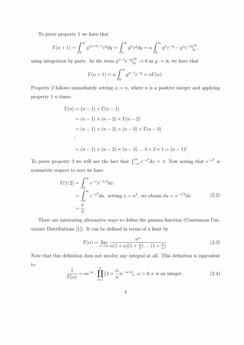
To prove property 1 we have that
Γ(α+ 1) =
∫∞
0
y(α+1)−1eydy =
∫∞
0
yαeydy = α
∫∞
0
yαe−y − yαe−y∣∣∞0,
using integration by parts. As the term yα−1e−y∣∣∞0
→ 0 as y → ∞ we have that
Γ(α+ 1) = α
∫∞
0
yα−1e−y = αΓ(α).
Property 2 follows immediately setting α = n, where n is a positive integer and applying
property 1 n times:
Γ(n) = (n− 1)× Γ(n− 1)
= (n− 1)× (n− 2)× Γ(n− 2)
= (n− 1)× (n− 2)× (n− 3)× Γ(n− 3)
...
= (n− 1)× (n− 2)× (n− 3) . . . 3× 2× 1 = (n− 1)!
To prove property 3 we will use the fact that∫∞
−∞e−x2
dx = π. Now noting that e−x2is
symmetric respect to zero we have
Γ(1/2) =
∫∞
0
e−xx−1/2dx.
=
∫∞
0
e−u2
du, setting x = u2, we obtain du = x−1/2dx
=π
2.
(2.2)
There are interesting alternative ways to define the gamma function (Continuous Uni-
variate Distributions [1]). It can be defined in terms of a limit by
Γ(α) = limn→∞
nα
α(1 + α)(1 + α2) . . . (1 + α
n). (2.3)
Note that this definition does not involve any integral at all. This definition is equivalent
to1
Γ(α)= αeγα ·
n∏
i=1
[(1 +α
n)e−α/n], α > 0, n is an integer , (2.4)
4
where γ is the Euler-Mascheroni constant given by
γ = limm→∞
[m∑
n=1
1
n− logm] ≈ 0.5772156649 . . . . (2.5)
The gamma function is studied in text of advanced calculus and arises often in applications.
2.3 Getting the Gamma Density
A function of the form
f(x) = cxα−1e−x/β, α, β > 0, (2.6)
defines a very special probability density. To find c we set∫
∞
0
cxα−1e−x/βdx = 1
Letting y = x/β the integral above becomes∫
∞
0
cxα−1e−x/βdx = cβα
∫∞
0
yα−1e−ydy = cβαΓ(α) = 1,
from where we get
c =1
βαΓ(α).
Now with this value for c the gamma density in (2.6) becomes
f(x, α, β) =1
βαΓ(α)xα−1e−x/β, α, β > 0. (2.7)
2.4 Mean, Variance and Moment Generating Func-
tion
We will use the notation X ∼ G(α, β) to denote that a random variable X with density
given by (2.7), follows a gamma distribution with parameters α, β.
The rth moment for the gamma distribution is given by
µ′
r = E(Xr) =βrΓ(α+ r)
Γ(α), α, β > 0, r a positive integer. (2.8)
5
The derivation for the rth moment comes from the definition
E(Xr) =1
βαΓ(α)
∫∞
0
xα−1 · xre−x/βdx
=1
βαΓ(α)
∫∞
0
xα+r−1e−x/βdx
=1
βαΓ(α)Γ(α+ r)βα+r =
βrΓ(α+ r)
Γ(α).
Thus we have that the mean is equal to
µ′
1 = E(X) =βΓ(α+ 1)
Γ(α)=βαγ(α)
γ(α)= αβ. (2.9)
The variance is given by
V ar(X) = µ′
2 − (µ′
1)2 =
β2Γ(α + 2)
Γ(α)−(βΓ(α+ 1)
Γ(α)
)2= αβ2. (2.10)
The moment generating function for the gamma is given by
MX(t) = E(etX) =
∫∞
0
etx · 1
βαΓ(α)xα−1e−x/βdx, −∞ < t <∞. (2.11)
In order to get this moment generating function we will try to express the right side above
as a gamma density. We do the change of variable y = x(1− βt) then:
E(etX) =
∫∞
0
1
βαΓ(α)xα−1e−x(1−βt)/βdx
=
∫∞
0
1
βαΓ(α)
yα−1
(1− βt)α−1· 1
1− βte−ydy
=1
(1− βt)α−1· 1
1− βt· 1
βαΓ(α)
∫∞
0
yα−1e−ydy =1
(1− βt)α.
One application for the moment generating function of a gamma distribution is that
of the reprodcutive property. If X1 ∼ G(α1, β) and X2 ∼ G(α2, β) are independent with
respective densities
f1(x, α1, β) =1
βα1Γ(α1)xα1−1e−x/β, α1, β > 0 (2.12)
and
f2(x, α2, β) =1
βα2Γ(α2)xα2−1e−x/β, α1, β > 0, (2.13)
6
then X1 + X2 ∼ G(α1 + α2, β). That is, the density for the sum of the random variables
X1 +X2 is
fX1+X2(x, α1 + α2, β) =1
βα1+α2Γ(α1 + α2)xα1+α2−1e−x/β. (2.14)
This easily seen using the properties for the moment generating function. Note that
MX1+X2(t) =MX1(t) ·MX2(t) because X1 and X2 are independent. So we have
MX1+X2(t) =MX1(t) ·MX2(t) = (1− βt)−α1 · (1− βt)−α2 = (1− βt)−(α1+α2).
Here we use the fact that there exists a unique correspondence between moment gener-
ating function and distribution. This means that as MX1+X2(t) has the form of a moment
generating function for a gamma with parameters β, α1 + α2 then X1 +X2 has a gamma
distribution with parameters β and α1 + α2. We can even generalize this to k independent
gamma’s. Let Xi, . . . Xk be k independent random variables each one following a gamma
distribution with parameters (αi, β), i = 1, 2, . . . k. Then the moment generating function
for these k independent gamma is
MX1·...·Xk(t) =MX1(t) · . . .MXk
(t) = (1− βt)−α1 · . . . · (1− βt)−αk = (1− βt)−∑k
i=1 αi .
This is the moment generating function for a gamma with parameters∑k
i=1 αi and β. So
by the same reasoning as in the two parameters case we conclude that the random variable
X1 + . . . Xn has a gamma distribution with parameters (∑k
i=1 αi, β).
2.5 Particular Cases and Shapes
2.5.1 Standard Gamma
Several forms of the gamma density can be obtained by changing the parameters in (2.7).
We will analyze these forms and study them for some values. One of them is obtained by
setting β = 1 in (2.7). That is
f(x, α, 1) =1
Γ(α)xα−1 · e−x, x > 0, α > 0, (2.15)
7
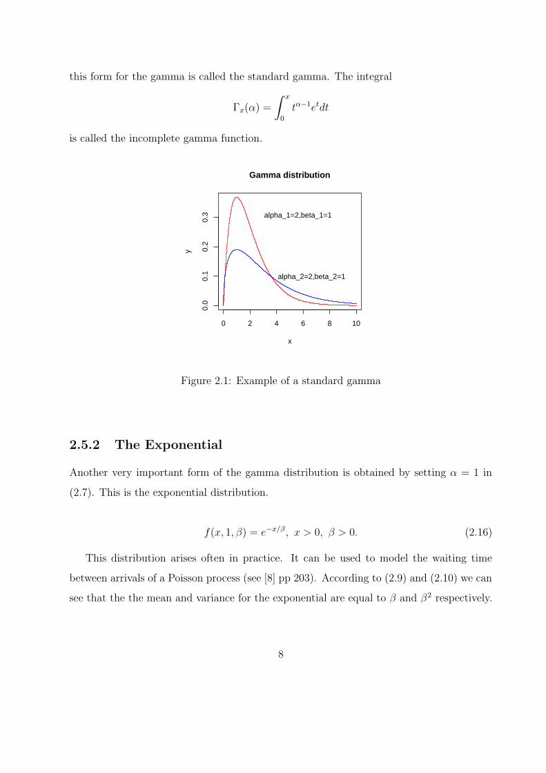
this form for the gamma is called the standard gamma. The integral
Γx(α) =
∫ x
0
tα−1etdt
is called the incomplete gamma function.
0 2 4 6 8 10
0.0
0.1
0.2
0.3
Gamma distribution
x
y
alpha_1=2,beta_1=1
alpha_2=2,beta_2=1
Figure 2.1: Example of a standard gamma
2.5.2 The Exponential
Another very important form of the gamma distribution is obtained by setting α = 1 in
(2.7). This is the exponential distribution.
f(x, 1, β) = e−x/β, x > 0, β > 0. (2.16)
This distribution arises often in practice. It can be used to model the waiting time
between arrivals of a Poisson process (see [8] pp 203). According to (2.9) and (2.10) we can
see that the the mean and variance for the exponential are equal to β and β2 respectively.
8
2 4 6 8 10 12
0.00
0.05
0.10
0.15
0.20
Gamma distribution
x
y
red.−alpha_1=1,beta_1=1
blue.−alpha_2=1,beta_2=2
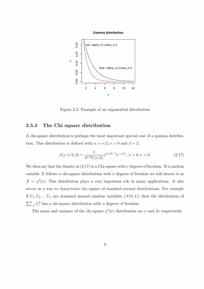
Figure 2.2: Example of an exponential distribution
2.5.3 The Chi square distribution
A chi-square distribution is perhaps the most important special case of a gamma distribu-
tion. This distribution is defined with α = ν/2, ν > 0 and β = 2.
f(x, ν/2, 2) =1
2ν/2Γ(ν/2)x(ν/2)−1e−x/2 , x > 0, ν > 0. (2.17)
We then say that the density in (2.17) is a Chi-square with ν degrees of freedom. If a random
variable X follows a chi-square distribution with ν degrees of freedom we will denote it as
X ∼ χ2(ν). This distribution plays a very important role in many applications. It also
serves as a way to characterize the square of standard normal distributions. For example
if U1, U2 . . . Un are standard normal random variables (N(0, 1)) then the distribution of∑n
i=1 U2i has a chi-square distribution with n degrees of freedom.
The mean and variance of the chi square χ2(ν) distribution are ν and 2ν respectively.
9
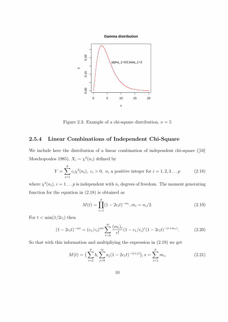
0 5 10 15 20
0.00
0.10
0.20
Gamma distribution
x
y
alpha_1=5/2,beta_1=2
Figure 2.3: Example of a chi-square distribution, ν = 5
2.5.4 Linear Combinations of Independent Chi-Square
We include here the distribution of a linear combination of independent chi-square ([10]
Moschopoulos 1985), Xi ∼ χ2(ni) defined by
Y =
p∑
i=1
ciχ2(ni), ci > 0, ni a positive integer for i = 1, 2, 3 . . . p (2.18)
where χ2(ni), i = 1 . . . p is independent with ni degrees of freedom. The moment generating
function for the equation in (2.18) is obtained as
M(t) =
p∏
i=1
(1− 2cit)−mi ,mi = ni/2. (2.19)
For t < min(1/2ci) then
(1− 2cit)−mi = (c1/ci)
mi
∞∑
r=0
(mi)rr!
(1− c1/ci)r(1− 2cit)
−(r+mr). (2.20)
So that with this information and multipliying the expression in (2.19) we get
M(t) =( p∑
i=2
bi
∞∑
j=0
aj(1− 2c1t)−(s+j)
), s =
p∑
i=1
mi, (2.21)
10
with
bi = (c1/ci)mi and A(i, r) = (mi)r(1− c1/ci)
r/r!,
besides the ajs satisfy the relation
p∏
i=2
[∞∑
r=0
A(ci, r)x−r] =
∞∑
j=0
ajx−j.
From this we can get the ajs recursively that is
aj = A(p)j , A
(i)j =
j∑
k=0
Ai−1k A(ci, j − k) (2.22)
where i = 3, 4, . . . , p j = 0, 1, 2 . . . and for r = 0, 1, 2, . . .
A(2)r = A(C2, r).
And now we invert (2.21) term by term. Since the density corresponding to the factor
(1− 2c1t)−(s+j) is the gamma density gj(y) where
gj(y) = ys+j−1e−y/2c1/(2c1)s+jΓ(s+ j)
the density function F (w) = P (Y ≤ w) (the probability that the random variable Y is less
or equal than w) is
F (w) =( p∏
i=2
bi) ∞∑
j=0
aj
∫∞
0
gj(y)dy. (2.23)
([10] Moschopoulos 1985).
11
Chapter 3
Estimation of Parameters
3.1 Method of Moments
We know from (2.8) that the r-th moment for X ∼ G(α, β) is given by
µ′
r =βrΓ(α + r)
Γ(α),
these are the population moments for r = 1, 2, 3 . . ..
If we consider random variables X1, X2, . . . Xn ∼ G(α, β), and if we observe a particular
value from each, x1, x2, . . . xn, then the sample moments are given by
∑ni=1 x
ri
n. The method
of moments consists on setting those population moments equal to the sample moments.
Considering the cases r = 1, 2, we must solve the equations
βΓ(α+ 1)
Γ(α)=
∑ni=1 xin
(3.1)
andβ2Γ(α+ 2)
Γ(α)=
∑ni=1 x
2i
n(3.2)
for β and α.
By using the properties for the gamma function (3.1) and (3.2) become
αβ =
∑ni=1 xin
, (3.3)
β2(α+ 1)α =
∑ni=1 x
2i
n. (3.4)
Solving (3.3) for β we obtain β =x
α, where x =
∑ni=1 xin
. Now if we substitute in (3.4) for
12
α we have
β2(α + 1)α =
∑ni=1 x
2i
n
⇔ x2
α2(α + 1)α =
∑ni=1 x
2i
n( substituing β =
x
α)
⇔ x2(α + 1)
α=
∑ni=1 x
2i
n
⇔ (α + 1)
α=
∑ni=1 x
2i
x2n
⇔ 1 +1
α=
∑ni=1 x
2i
x2n
⇔ 1
α=
∑x2i
xn− 1 =
∑x2i − x2n
x2n,
from where finally we get
α =x2n∑x2i − x2n
and
β =x
α
3.2 Maximum Likelihood Estimation
Let X1, X2, . . . Xn ∼ G(α, β) for i = 1, 2 . . . n. The likelihood function is given by
L(x1, . . . xn, α, β) =n∏
i=1
f(xi, α, β) =1
Γ(α)n · βnα(x1, . . . xn)
α−1e−∑n
i=1(xi/β). (3.5)
The maximum likelihood estimation method consists on finding the values for α and β such
that (3.5) is a minimum.
Taking natural log at both sides of (3.5) and using the properties for logarithms we
have
ln(L(x1 . . . xn, α, β)) = −n ln(Γ(α))− nα ln(β) + (α− 1) ln(x1, . . . xn)−Σni=1(xi/β). (3.6)
The derivative respect to α in (3.6) set it equal to zero give the corresponding equation
∂L
∂α= −nΓ
′(α)
Γ(α)− n ln(β) +
n∑
i=1
ln(xi) = 0.
13
This can be expressed as
∂L
∂α= −nΓ
′(α)
Γ(α)+
n∑
i=1
(ln(xi)− ln(β)
)= 0
= −nΓ′(α)
Γ(α)+
n∑
i=1
ln(xi/β) = 0.
(3.7)
Differentiating with respect to β
∂L
∂β= −−nα
β+
∑ni=1 xiβ2
. (3.8)
Setting (3.8) equal to zero the equation is
− −nαβ
+
∑ni=1 xiβ2
= 0
⇔ −nα +
∑ni=1 xiβ
= 0
⇔∑n
i=1 xiβ
= nα.
From where we obtain
β =
∑ni=1 xinα
=x
α. (3.9)
Where we have used the notation β to denote the maximum likelihood estimator for β.
Try to solve for α the equation (3.7) is quite complicated because of the function Γ(α).
There is no closed way to solve for α in this equation. By adding the value for β in terms
of α obtained in (3.9) to (3.7) we get
− nΓ′(α)
Γ(α)+
n∑
i=1
ln(xi/β) = −nΓ′(α)
Γ(α)+
n∑
i=1
ln(xiα/x)
= −nnΓ′(α)
Γ(α)+
n∑
i=1
(ln(xi) + ln(α)− ln(x)
)
= −nψ(α) +n∑
i=1
ln(xi) + n ln(α)− n ln(x)
= −ψ(α) +∑n
i=1 ln(xi)
n+ ln(α)− ln(x) = 0
⇔ ln(α)− ψ(α) = ln(x)−∑n
i=1 ln(xi)
n,
(3.10)
14
where ψ(α) is the digamma function defined as ψ(α) = Γ′(α)Γ(α)
. One approximation for the
left side of (3.10) is
ln(α)− ψ(α) ≈ 1
α
(12+
1
12α + 2
).
So (3.10) becomes1
α
(12+
1
12α + 2
)≈ ln(x)−
∑ni=1 ln(xi)
n.
Finally solving this equation for α we obtain the approximate maximum likelihood estima-
tion for α
α ≈ 3− s+√(s− 3)2 + 24s
12s(3.11)
where s = ln(x)− 1n
∑ni=1 ln(xi) ([5] S. C. Choi and R. Wette. (1969)).
3.3 Applications
Now we will use the previous estimators to fit a gamma density to a set of data.
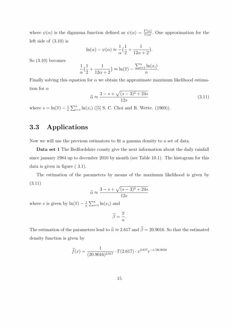
Data set 1 The Bedfordshire county give the next information about the daily rainfall
since january 1984 up to december 2010 by month (see Table 10.1). The histogram for this
data is given in figure ( 3.1).
The estimation of the parameters by means of the maximum likelihood is given by
(3.11)
α ≈ 3− s+√(s− 3)2 + 24s
12s
where s is given by ln(x)− 1n
∑ni=1 ln(xi) and
β =x
α.
The estimation of the parameters lead to α ≈ 2.617 and β = 20.9016. So that the estimated
density function is given by
f(x) =1
(20.9016)2.617· Γ(2.617) · x2.617e−x/20.9016
15
Bedfordshire Rainfall
data
Den
sity
0 50 100 150
0.00
00.
004
0.00
80.
012
Figure 3.1: Relative Frequency Histogram of Bedfordshire Rainfall
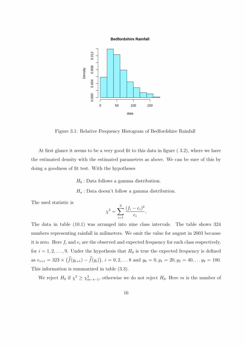
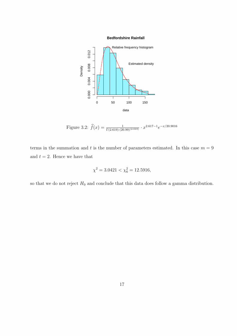
At first glance it seems to be a very good fit to this data in figure ( 3.2), where we have
the estimated density with the estimated parameters as above. We can be sure of this by
doing a goodness of fit test. With the hypotheses
H0 : Data follows a gamma distribution.
Ha : Data doesn’t follow a gamma distribution.
The used statistic is
χ2 =9∑
i=1
(fi − ei)2
ei,
The data in table (10.1) was arranged into nine class intervals. The table shows 324
numbers representing rainfall in milimeters. We omit the value for august in 2003 because
it is zero. Here fi and ei are the observed and expected frequency for each class respectively,
for i = 1, 2, . . . , 9. Under the hypothesis that H0 is true the expected frequency is defined
as ei+1 = 323 ×(f(yi+1) − f(yi)
), i = 0, 2, . . . 8 and y0 = 0, y1 = 20, y2 = 40, . . . y9 = 180.
This information is summarized in table (3.3).
We reject H0 if χ2 ≥ χ2m−t−1, otherwise we do not reject H0. Here m is the number of
16
Bedfordshire Rainfall
data
Den
sity
0 50 100 150
0.00
00.
004
0.00
80.
012
Estimated density
Relative frequency histogram
Figure 3.2: f(x) = 1Γ(2.619)·(20.99)(2.619)
· x2.617−1e−x/20.9016
terms in the summation and t is the number of parameters estimated. In this case m = 9
and t = 2. Hence we have that
χ2 = 3.0421 < χ26 = 12.5916,
so that we do not reject H0 and conclude that this data does follow a gamma distribution.
17
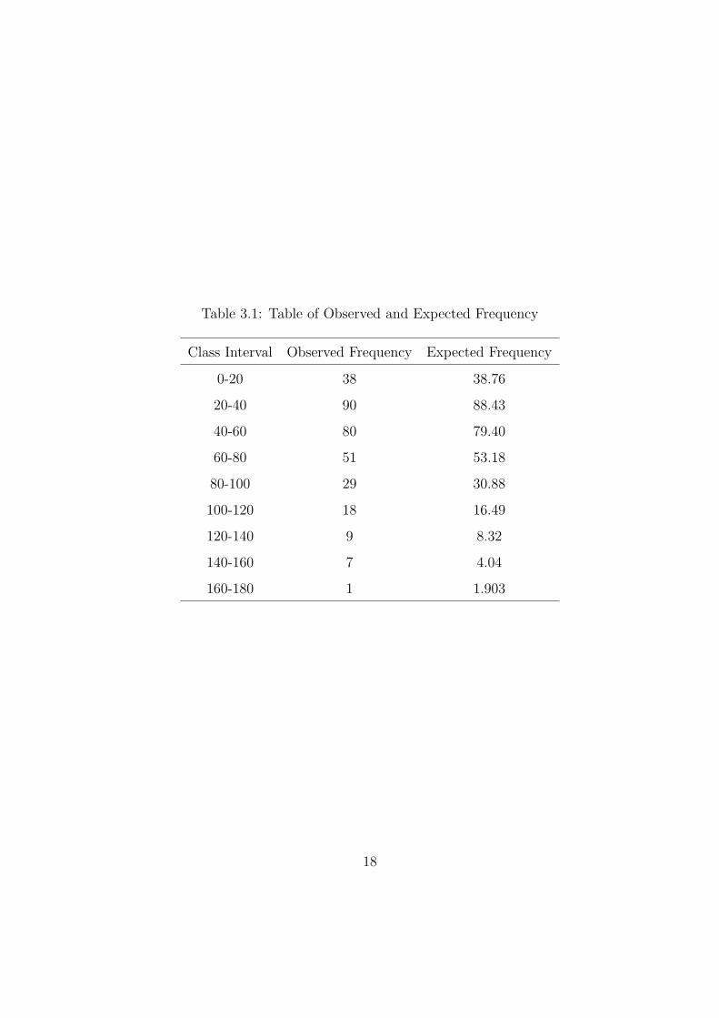
Table 3.1: Table of Observed and Expected Frequency
Class Interval Observed Frequency Expected Frequency
0-20 38 38.76
20-40 90 88.43
40-60 80 79.40
60-80 51 53.18
80-100 29 30.88
100-120 18 16.49
120-140 9 8.32
140-160 7 4.04
160-180 1 1.903
18
Chapter 4
Distributions Related to the Gamma
Distributions
4.1 Log Gamma Distribution
We say that a random variable X is log gamma distributed if ln(X) is gamma distributed.
This means that if Y = ln(X) then the density for Y denoted by f(y, α, β) is given by
fY (y, α, β) =1
βα · Γ(α)yα−1e−y/β, β, α, y > 0. (4.1)
We will get the density for X. Noting that Y is a transformation for X the density for X is
given by f(x, α, β) = fY (ln(x)) ·∣∣dydx
∣∣. As we know that ln(x) = y and∣∣dydx
∣∣ = 1
xwe obtain
f(x, α, β) =(ln(x))α−1
xβαΓ(α)· e− ln(x)/β
=(ln(x))α−1
xβαΓ(α)· x−1/β =
(ln(x))α−1
βαΓ(α)· x−(β+1)/β, x > 1.
Some properties ([6] P.C Consul and G. C. Jain) for the log gamma distribution are:
1. If Y is a log gamma with density f(x, α, β) then Y n is also a log gamma distribution
with density f(x, α/n, β).
2. If Y1, Y2, . . . Yn are independent log gamma variables with densities f(xi, α, βi) for
i = 1, 2 . . . , then U = Πni=1Yi is also a log gamma density with density f(u, α,
∑ni=1 βi).
3. If Y1, Y2, . . . Yn is a sequence of independent log gamma variables, where Yi has density
f(xi, α, βi) for all i = 1, 2 . . . , then the product U = Πni=1Y
ni is also a log gamma
variable with density f(u, α/n,∑n
i=1 βi).
19
4.2 The Quotient of Two Independent Gamma
Now if we consider the ratio X/Y , where X ∼ G(α1, β1) and Y ∼ G(α2, β2) and they are
independent. Setting
u = X + Y, v =X
Y,
then the jacobian becomes |J | = −(1−v)2
u. So
fU,V (u, v) =1
Γ(α1)Γ(α2)e−u
( uv
1 + v
)α1−1( u
1 + v
)α2−1 u
1 + v
2
=1
Γ(α1)Γ(α2)e−uuα1+α2−1vα2−1(1 + v)−(α1+α2).
If we integrate this with respect to u we obtain
fV (v) =1
Γ(α1)Γ(α2)
∫∞
0
e−uuα1+α2−1vα2−1(1 + v)−(α1+α2)du
=1
Γ(α1)Γ(α2)vα2−1(1 + v)−(α1+α2)
∫∞
0
e−uuα1+α2−1du
=1
Γ(α1)Γ(α2)vα2−1(1 + v)−(α1+α2)Γ(α1 + α2),
because
∫∞
0
e−uuα1+α2−1du = Γ(α1 + α2).
4.3 The QuotientX1
X1 +X2
If X1 and X2 are independent random gamma variables with parameters (α1, β) and (α2, β)
respectiveley, then X1/(X1 +X2) has a beta distribution with parameters α1, α2. We can
deduce this from
f(x1) =1
βα11 · Γ(α1)
xα1−11 e−x/β,
f(x2) =1
βα22 · Γ(α2)
xα2−11 e−x/β,
then as the random variables are independent we have
f(x1, x2) =1
Γ(α1) · Γ(α2)
1
βα1· 1
βα2e
−(x1+x2)β xα1−1
1 xα2−12 . (4.2)
20
Now we set
u = X1 +X2, v = X1/(X1 +X2),
then
X1 = uv, X2 = u(1− v).
With this the jacobian becomes |J | = u. So
fU.V (u, v) =u
Γ(α1)Γ(α2)e−u/β · (uv)α1−1uα2−1(1− v)α2−1
=u
Γ(α1)Γ(α2)e−u/βuα1+α2−1vα1−1(1− v)α2−1.
(4.3)
Therefore, integrating (4.3) respect to v the sum has distribution
f(u) =e−u/βuα1+α2−1
Γ(α1 + α2),
which is a gamma distribution with parameters α1 + α2 and β. Now using (4.3) and
integrating respect to u the ratio v = X1/(X1 +X2) has distribution
fV (v) =Γ(α1 + α2)
Γ(α1) · Γ(α2)vα1−1 · (1− v)α2−1,
which is a beta function with parameters α1, α2.
4.4 Sum of k Independent Gamma
We can say even more about the random variable Y =∑k
i=1Xi where each variable has
gamma distribution, that is Xi ∼ (αi, βi), i = 1, 2 . . . n and they are independent ([9],
Moschopoulos 1985) . We can obtain the exact distribution for Y. We know that each Xi
has moment generating function given by
M(t) = (1− βit)−αi ,
then Y has moment generating function given by
M(t) =k∏
i=1
(1− βit)−αi .
21
The idea is to express M(t) as
M(t) = C(1− βit)−ρ · exp(
∞∑
k=1
γk(1− βit)−k),
where exp(a) = ea and
C =∏
(β1/βi)αi ,
with β1 = min(β1, β2 . . . βn) (the minimum among all β ′s),
γk =n∑
i=1
αi(1− β1/βi)k/k,
ρ =n∑
i=1
αi > 0.
And now if we let
exp(∞∑
k=1
γk(1− βit)−k) =
∞∑
k=0
δk(1− β1t)−k.
By differentiating with respect to (1− βt)−1, the coefficients δk can be obtained by means
of the formula
δk+1 =1
k + 1
k+1∑
i=1
iγiδk+1−i.
This leads to the next theorem which gives an expression for Y ([9] Moschopoulos 1985).
Theorem 1. If Xi ∼ (α1, βi) and independently distributed for i = 1, 2, . . . n. Then the
density for Y can be expressed as
g(y) = C∞∑
k=0
δkyρ+k−1e−y/β1/[Γ(ρ+ k)βρ+k
1 ], y > 0 (4.4)
and 0 elsewhere.
22
4.4.1 Aprroximation for the Exact Distribution of the sum of k
Independent Gamma
Approximation with Two Moments
If Xi ∼ G(αi, βi) for i = 1 . . . n, and Y = X1 + . . .+Xn. Then we know that the density is
given by (4.4)
g(y) = C∞∑
k=0
δkyρ+k−1e−y/β1/[Γ(ρ+ k)βρ+k
1 ], y > 0. (4.5)
If we want to compute G(y), the distribution for this sum, we need to evaluate this
inifinite sum. But we can approximate it assuming that Y ∼ G(α, β) and knowing two
moments of this assumed distribution. If Y ∼ G(α, β) then EY = αβ and V ar(Y ) = αβ2,
from where we obtain
β =V ar(Y )
E(Y ),
and
α =E(Y )2
V ar(Y ),
but E(Y ) = α1β1 + α2β2 + . . . αnβn and V ar(Y ) = α1β21 + . . . + αnβ
2n. So that with these
values we obtain assuming that Y ∼ G(α, β)
β =α1β
21 + . . .+ αnβ
2n
α1β1 + α2β2 + . . . αnβn
and
α =(α1β1 + α2β2 + . . . αnβn)
2
(α1β21 + . . .+ αnβ2
n).
If we use this values for α and β we can approximate (4.5) with G(α, β), where α and
β are given as above.
Normal Approximation
If Xi, i = 1 . . . n are independent standard normal variables and considering the following
linear combination ([18] Solomon and Jensen 1972)
Qk(c, a) =k∑
j=1
cj(x2j + aj), cj > 0, 1 ≥ j ≤ k, (4.6)
23
then the sth cumulant of Qk(c, a) is
κs = 2s−1(s− 1)!k∑
j=1
csj(1 + sa2j).
Under the condition that the parameters cj, aj are bounded, it can be shown that the dis-
tribution of Qk tends to a gaussian distribution as θ1 → ∞ where θ1 = E(Qk(c, a)). So
following this idea (Solomon and Jensen 1972) used the transformation (Qk/θ1)h to accel-
erate the rate of convergence and thus to provide a Gaussian approximation for moderate
values of θ1. The moments of (Qk/θ1)h expanded in powers of (θ1)
−1 were obtained. In
particular the third central moment is
µ3(h) =4h2
θ21
(2φ3 + 3(h− 1)φ2
2
)
h2(h− 1)
θ31
(72φ4 + 24(7h− 10)φ2φ3
)
+ 4(17h2 − 55h+ 44)φ22 + 0(θ−4
1 ),
(4.7)
where φr = θr/θ1, r = 2, 3. A similar expression for γ1, the skewness of (Qk/θ1)h is
γ1(h) =4(2φ3 + 3(h− 1)φ2
2
)
θ1/21 (2φ
3/22 )
· (h− 1)(72φ4 + 24(7h− 10)φ2φ3 +
4(17h2 − 55h+ 44)φ32
)
θ5/21
+ 0(θ−5/21 ).
(4.8)
Now h is chosen so that the leading term in γ1 and µ3 vanishes. This is
2θ3θ1
+ 3(h− 1)(θ2θ1
)2= 0. (4.9)
This yields to
h = 1− 2θ1θ33θ22
. (4.10)
Now the distribution of the random variable (Qk/θ1)h can be approximated by a Gaussian
distribution with mean
µ′
1(h) = 1 + θ2h(h− 1)/θ21, (4.11)
24
and variance
V ar(Qk/θ1)h(h) = 2θ2h2/θ1. (4.12)
In summary the variable z = θ1((Qk/θ1)
h − 1− θ2h(h− 1)/θ21)/(2θ2h
2) is approximately a
standard normal variable.
Now, motivated with this ideas, we will consider another approximation for the distri-
bution of Y = X1+X2+ . . . Xn, with Xi ∼ G(αi, βi), i = 1, 2 . . . n.We propose that (Y/θ1)h
with h given as in (4.10) and E(Y ) = θ1, can be approximated with a standard normal
distribution with mean µh and variance σ2h given as follows. We introduce the cumulant κn
of the random variable Y defined as
κn = g(n)(t) =dn
dtg(t),
where
g(t) = ln(E(etY )
)= −
∞∑
n=1
1
n
(1− E(etY )
)n
=∞∑
n=1
1
n
(−
∞∑
m=1
µ′
m
tm
m!
)n
= µ′
1t+(µ′
2 − µ′
1
)t22!
+(µ′
3 − 3µ′
2µ′
1 + 2(µ′
1)3)t33!
+ . . . .
We have used the fact that ln(x) = −∑
∞
n=1(1−x)n
n
Hence we have that
κ1 = g′(0) = µ′,
κ2 = g′′(0) = µ′
2 + (µ′
1)2,
κ3 = g(3)(0) = µ′
3 − 3µ′
2µ′
1 + 2(µ′
1)3.
In general κn = g(n)(0). Now if we define
h = 1− κ1κ3/(3 · κ21),
µh = 1 +h(h− 1) · φ2
2 · κ1+h · (h− 1) · (h− 2) · (4 · φ3 + 3 · (h− 3) · φ2
2)
24 · κ21
25
and
σ2h =
φ2h2
κ1+
(h− 1) · h2(2φ3 + (3h− 5)φ2
2
)
2κ21,
with
φ2 =κ2κ1,
φ3 =κ3κ1,
then we take
Z =((Y/θ1)h − µh
σh
)(4.13)
to be approximately a standardized Gaussian variable. So that we can use this information
to approximate the distribution of Y. This kind of approximation has been used in literature
with other applications. Moschopoulos in 1983 ([11]) and Moschopoulos and Mudholkar in
1983 ([12]) used and actually improved the efficiency of these approximations. In the next
pages tables with the normal and two moments approximation are shown. We consider
here the distribution P (Y ≤ t) where Y = X1 + . . .+Xn.
26
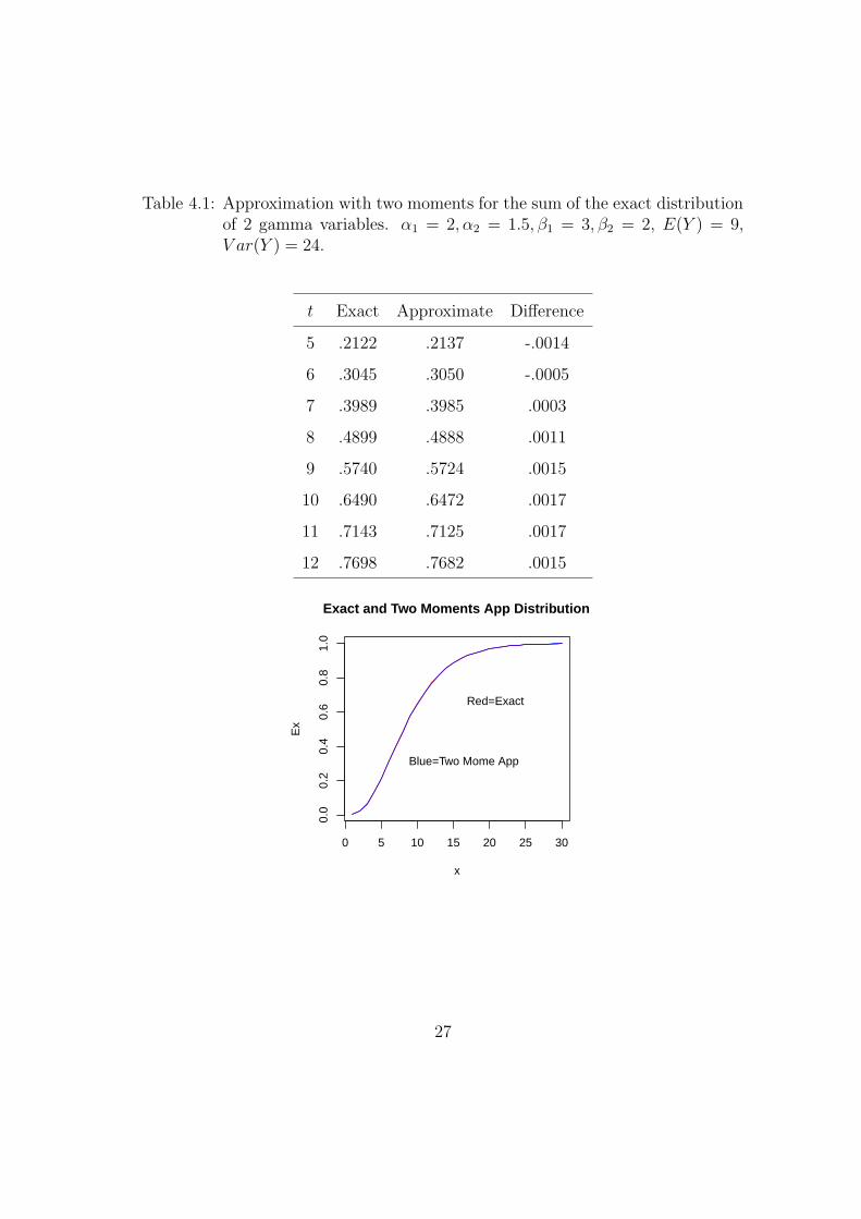
Table 4.1: Approximation with two moments for the sum of the exact distributionof 2 gamma variables. α1 = 2, α2 = 1.5, β1 = 3, β2 = 2, E(Y ) = 9,V ar(Y ) = 24.
t Exact Approximate Difference
5 .2122 .2137 -.0014
6 .3045 .3050 -.0005
7 .3989 .3985 .0003
8 .4899 .4888 .0011
9 .5740 .5724 .0015
10 .6490 .6472 .0017
11 .7143 .7125 .0017
12 .7698 .7682 .0015
0 5 10 15 20 25 30
0.0
0.2
0.4
0.6
0.8
1.0
Exact and Two Moments App Distribution
x
Ex
Red=Exact
Blue=Two Mome App
27
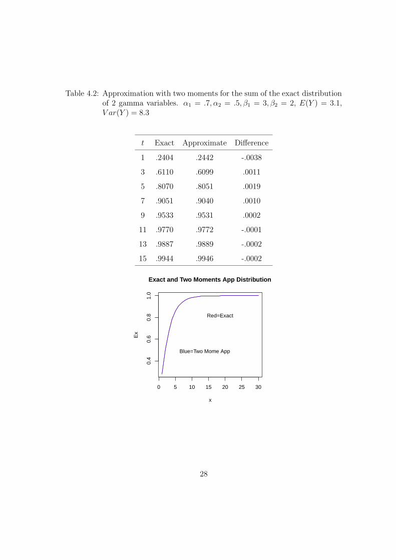
Table 4.2: Approximation with two moments for the sum of the exact distributionof 2 gamma variables. α1 = .7, α2 = .5, β1 = 3, β2 = 2, E(Y ) = 3.1,V ar(Y ) = 8.3
t Exact Approximate Difference
1 .2404 .2442 -.0038
3 .6110 .6099 .0011
5 .8070 .8051 .0019
7 .9051 .9040 .0010
9 .9533 .9531 .0002
11 .9770 .9772 -.0001
13 .9887 .9889 -.0002
15 .9944 .9946 -.0002
0 5 10 15 20 25 30
0.4
0.6
0.8
1.0
Exact and Two Moments App Distribution
x
Ex
Red=Exact
Blue=Two Mome App
28
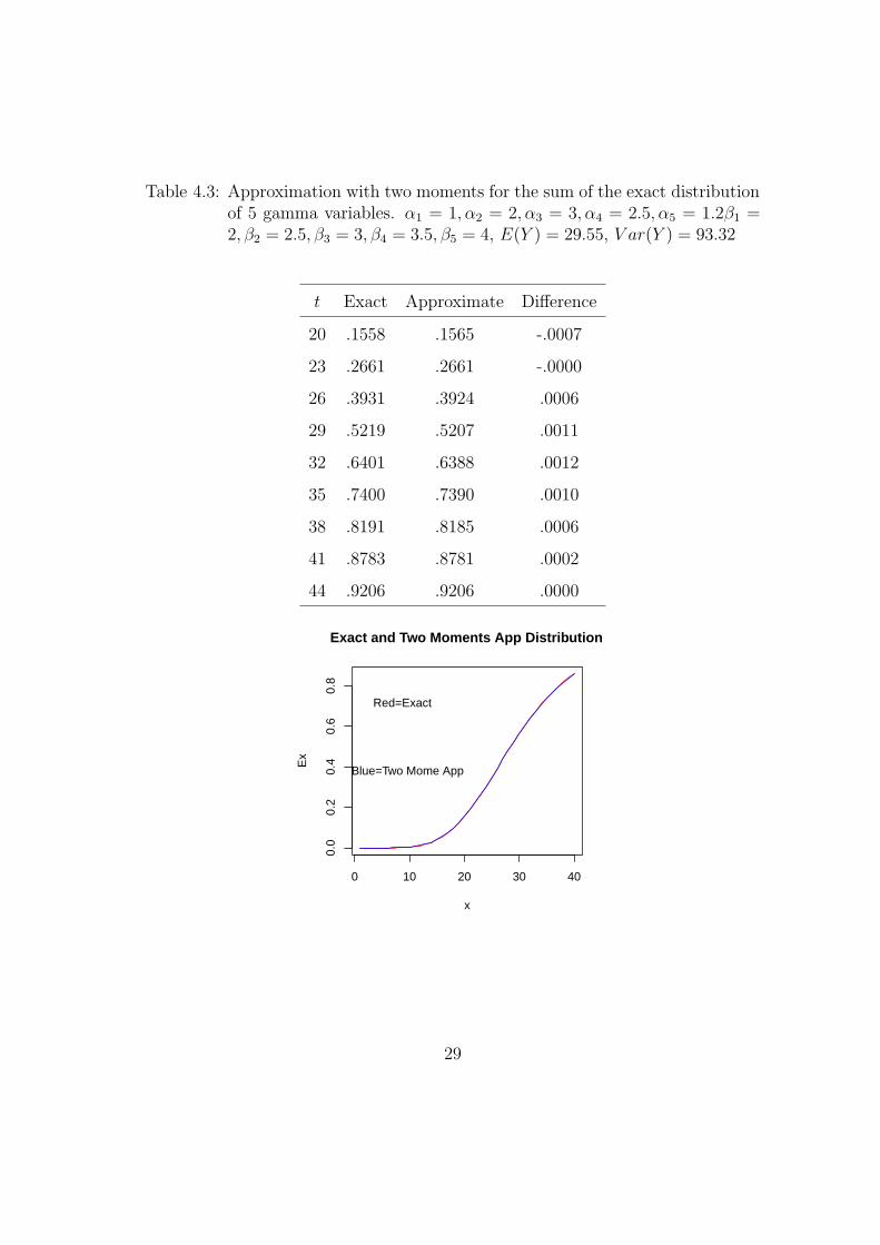
Table 4.3: Approximation with two moments for the sum of the exact distributionof 5 gamma variables. α1 = 1, α2 = 2, α3 = 3, α4 = 2.5, α5 = 1.2β1 =2, β2 = 2.5, β3 = 3, β4 = 3.5, β5 = 4, E(Y ) = 29.55, V ar(Y ) = 93.32
t Exact Approximate Difference
20 .1558 .1565 -.0007
23 .2661 .2661 -.0000
26 .3931 .3924 .0006
29 .5219 .5207 .0011
32 .6401 .6388 .0012
35 .7400 .7390 .0010
38 .8191 .8185 .0006
41 .8783 .8781 .0002
44 .9206 .9206 .0000
0 10 20 30 40
0.0
0.2
0.4
0.6
0.8
Exact and Two Moments App Distribution
x
Ex
Red=Exact
Blue=Two Mome App
29
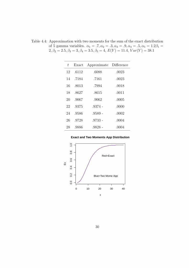
Table 4.4: Approximation with two moments for the sum of the exact distributionof 5 gamma variables. α1 = .7, α2 = .3, α3 = .9, α4 = .5, α5 = 1.2β1 =2, β2 = 2.5, β3 = 3, β4 = 3.5, β5 = 4, E(Y ) = 11.4, V ar(Y ) = 38.1
t Exact Approximate Difference
12 .6112 .6088 .0023
14 .7184 .7161 .0023
16 .8013 .7994 .0018
18 .8627 .8615 .0011
20 .9067 .9062 .0005
22 .9375 .9374 - .0000
24 .9586 .9589 - .0002
26 .9728 .9733 - .0004
28 .9886 .9828 - .0004
0 10 20 30 40
0.0
0.2
0.4
0.6
0.8
1.0
Exact and Two Moments App Distribution
x
Ex
Red=Exact
Blue=Two Mome App
30
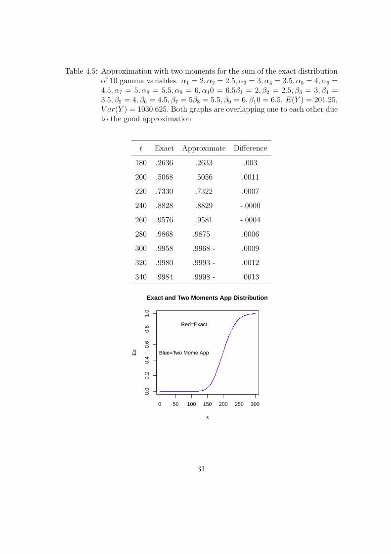
Table 4.5: Approximation with two moments for the sum of the exact distributionof 10 gamma variables. α1 = 2, α2 = 2.5, α3 = 3, α4 = 3.5, α5 = 4, α6 =4.5, α7 = 5, α8 = 5.5, α9 = 6, α10 = 6.5β1 = 2, β2 = 2.5, β3 = 3, β4 =3.5, β5 = 4, β6 = 4.5, β7 = 5β8 = 5.5, β9 = 6, β10 = 6.5, E(Y ) = 201.25,V ar(Y ) = 1030.625. Both graphs are overlapping one to each other dueto the good approximation
t Exact Approximate Difference
180 .2636 .2633 .003
200 .5068 .5056 .0011
220 .7330 .7322 .0007
240 .8828 .8829 -.0000
260 .9576 .9581 -.0004
280 .9868 .9875 - .0006
300 .9958 .9968 - .0009
320 .9980 .9993 - .0012
340 .9984 .9998 - .0013
0 50 100 150 200 250 300
0.0
0.2
0.4
0.6
0.8
1.0
Exact and Two Moments App Distribution
x
Ex
Red=Exact
Blue=Two Mome App
31
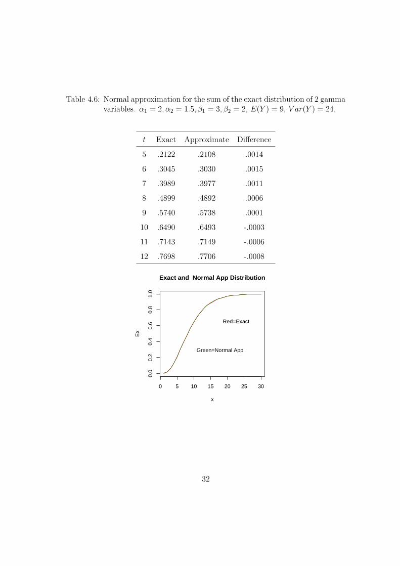
Table 4.6: Normal approximation for the sum of the exact distribution of 2 gammavariables. α1 = 2, α2 = 1.5, β1 = 3, β2 = 2, E(Y ) = 9, V ar(Y ) = 24.
t Exact Approximate Difference
5 .2122 .2108 .0014
6 .3045 .3030 .0015
7 .3989 .3977 .0011
8 .4899 .4892 .0006
9 .5740 .5738 .0001
10 .6490 .6493 -.0003
11 .7143 .7149 -.0006
12 .7698 .7706 -.0008
0 5 10 15 20 25 30
0.0
0.2
0.4
0.6
0.8
1.0
Exact and Normal App Distribution
x
Ex
Red=Exact
Green=Normal App
32
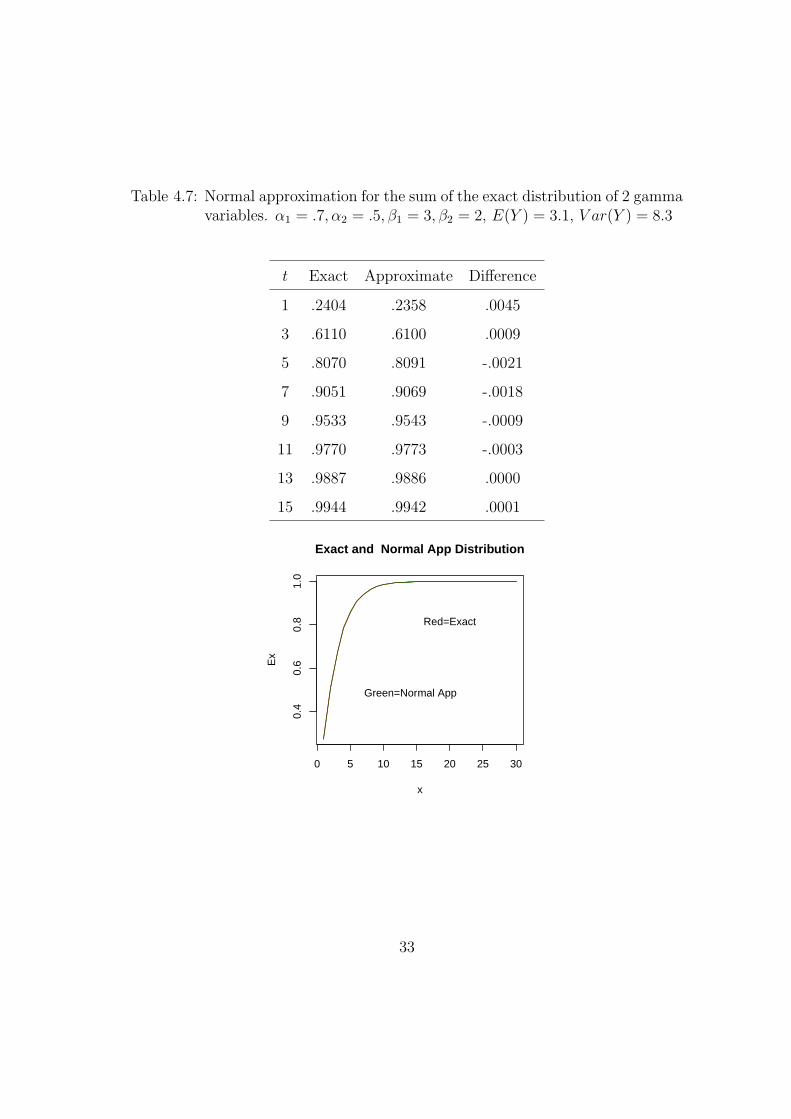
Table 4.7: Normal approximation for the sum of the exact distribution of 2 gammavariables. α1 = .7, α2 = .5, β1 = 3, β2 = 2, E(Y ) = 3.1, V ar(Y ) = 8.3
t Exact Approximate Difference
1 .2404 .2358 .0045
3 .6110 .6100 .0009
5 .8070 .8091 -.0021
7 .9051 .9069 -.0018
9 .9533 .9543 -.0009
11 .9770 .9773 -.0003
13 .9887 .9886 .0000
15 .9944 .9942 .0001
0 5 10 15 20 25 30
0.4
0.6
0.8
1.0
Exact and Normal App Distribution
x
Ex
Red=Exact
Green=Normal App
33
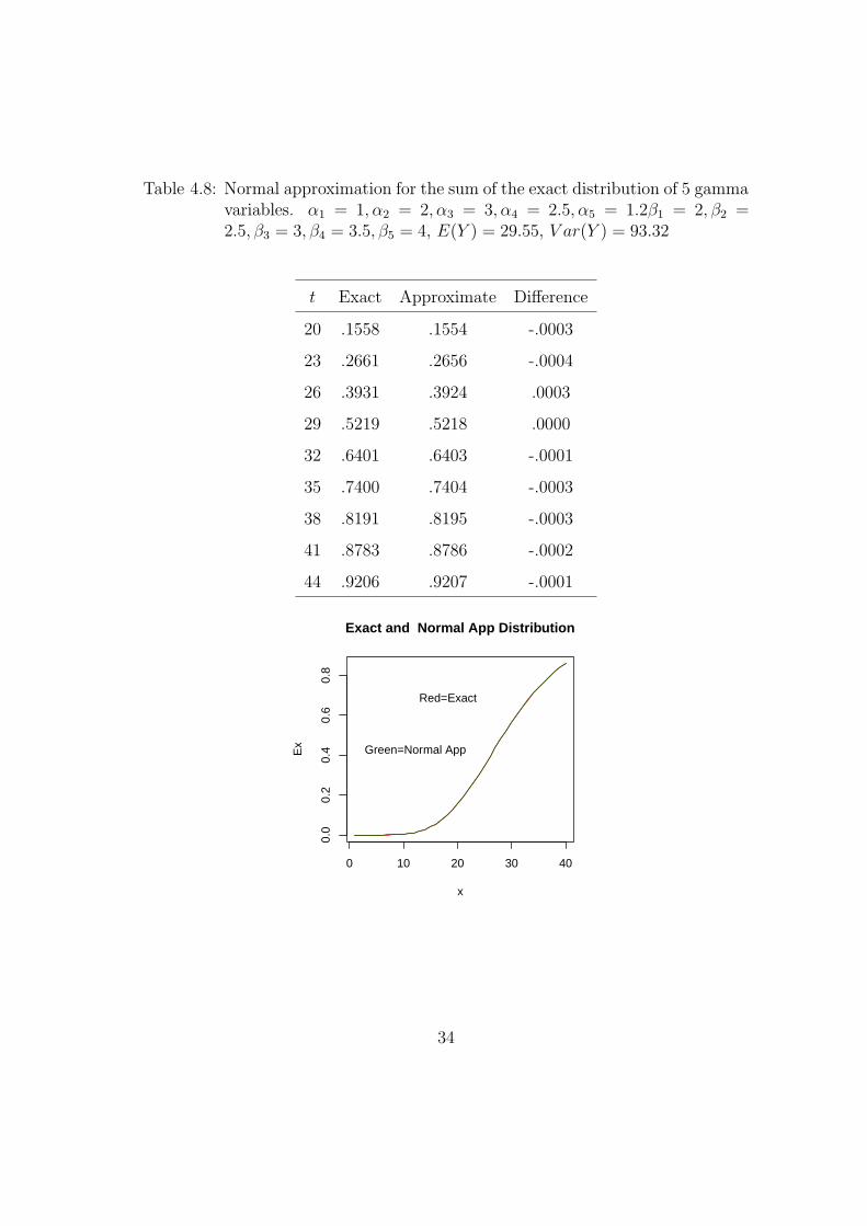
Table 4.8: Normal approximation for the sum of the exact distribution of 5 gammavariables. α1 = 1, α2 = 2, α3 = 3, α4 = 2.5, α5 = 1.2β1 = 2, β2 =2.5, β3 = 3, β4 = 3.5, β5 = 4, E(Y ) = 29.55, V ar(Y ) = 93.32
t Exact Approximate Difference
20 .1558 .1554 -.0003
23 .2661 .2656 -.0004
26 .3931 .3924 .0003
29 .5219 .5218 .0000
32 .6401 .6403 -.0001
35 .7400 .7404 -.0003
38 .8191 .8195 -.0003
41 .8783 .8786 -.0002
44 .9206 .9207 -.0001
0 10 20 30 40
0.0
0.2
0.4
0.6
0.8
Exact and Normal App Distribution
x
Ex
Red=Exact
Green=Normal App
34
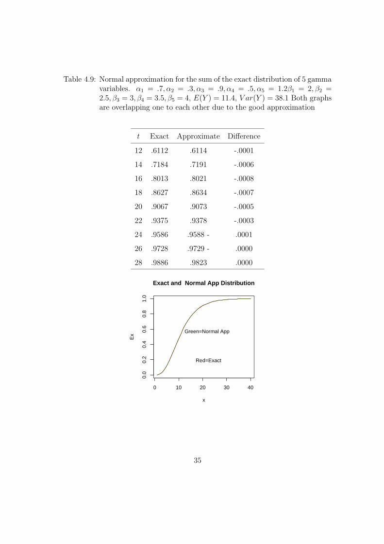
Table 4.9: Normal approximation for the sum of the exact distribution of 5 gammavariables. α1 = .7, α2 = .3, α3 = .9, α4 = .5, α5 = 1.2β1 = 2, β2 =2.5, β3 = 3, β4 = 3.5, β5 = 4, E(Y ) = 11.4, V ar(Y ) = 38.1 Both graphsare overlapping one to each other due to the good approximation
t Exact Approximate Difference
12 .6112 .6114 -.0001
14 .7184 .7191 -.0006
16 .8013 .8021 -.0008
18 .8627 .8634 -.0007
20 .9067 .9073 -.0005
22 .9375 .9378 -.0003
24 .9586 .9588 - .0001
26 .9728 .9729 - .0000
28 .9886 .9823 .0000
0 10 20 30 40
0.0
0.2
0.4
0.6
0.8
1.0
Exact and Normal App Distribution
x
Ex
Red=Exact
Green=Normal App
35
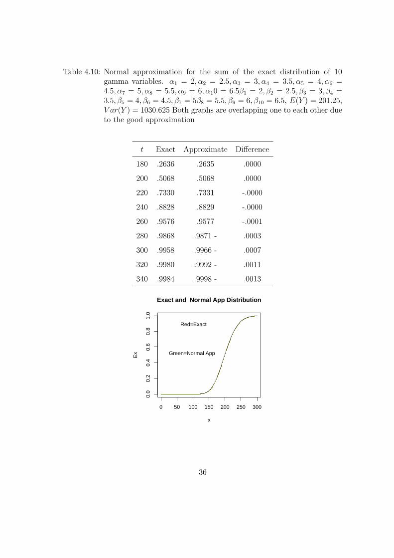
Table 4.10: Normal approximation for the sum of the exact distribution of 10gamma variables. α1 = 2, α2 = 2.5, α3 = 3, α4 = 3.5, α5 = 4, α6 =4.5, α7 = 5, α8 = 5.5, α9 = 6, α10 = 6.5β1 = 2, β2 = 2.5, β3 = 3, β4 =3.5, β5 = 4, β6 = 4.5, β7 = 5β8 = 5.5, β9 = 6, β10 = 6.5, E(Y ) = 201.25,V ar(Y ) = 1030.625 Both graphs are overlapping one to each other dueto the good approximation
t Exact Approximate Difference
180 .2636 .2635 .0000
200 .5068 .5068 .0000
220 .7330 .7331 -.0000
240 .8828 .8829 -.0000
260 .9576 .9577 -.0001
280 .9868 .9871 - .0003
300 .9958 .9966 - .0007
320 .9980 .9992 - .0011
340 .9984 .9998 - .0013
0 50 100 150 200 250 300
0.0
0.2
0.4
0.6
0.8
1.0
Exact and Normal App Distribution
x
Ex
Red=Exact
Green=Normal App
36
Chapter 5
Generalized Gamma Distributions
5.1 History
Generalized gamma distributions were discussed since the beginning of the 20th century. It
appeared when fitting such distribution to an observed distribution of income rates. There
was not a good interest in this kind of distribution up to the middle of the 20th century.
From that time on, the interest in the generalized gamma was increasing. Properties,
applications, distributions which were related to a generalized gamma were showing up.
Stacy (see [15] 1963) published a paper which developed the idea of a generalized gamma
introducing basic properties. It was the first paper talking entirely about this generalized
distribution.
5.2 Motivation and Getting the Generalized Gamma
Density
So far we have seen several properties for the gamma distribution. We will focus our
attention on investigating the properties of the generalized gamma functions. If X is a
random variable we say X has generalized gamma density if its pdf is given by
f(x) = cxδα−1e−( xβ)δ , x, α, β, δ > 0. (5.1)
This distribution contains all previous densities we have just seen, such as gamma
density and its densities derived from it. This is one form of the generalized gamma
37
that appears often in literature (see [1]), but there exist others forms that depend on the
parameters. This is form is convenient for our purposes.
The constant c in (5.1) is the reciprocal of the integral∫
∞
0
xδα−1e−( xβ)δdx.
If we let y = (x/β)δ we get xδα−1 = yα−1δ · βδα−1. And the differential dx is given by
dx = (β/δ) · y 1−δδ .
And then we get∫
∞
0
cxδα−1e−( xβ)δdx = βδα · 1
δ
∫∞
0
cyα−1δ+ 1
δ−1e−ydy = βδα · 1
δ
∫∞
0
cyα−1e−ydy = 1.
But as ∫∞
0
yα−1e−ydy
has the form of a standard gamma we obtain∫
∞
0
yα−1e−ydy = Γ(α).
Finally have
βδα · 1δ
∫∞
0
cyα−1e−ydy = βδα · 1δcΓ(α) = 1.
From where we get
c =δ
βδαΓ(α).
And thus the generalized gamma density becomes
f(x, α, β, δ) =δ
βδαΓ(α)· xδα−1e−( x
β)δ . (5.2)
5.3 Basic Properties for the Generalized Gamma Dis-
tribution
We will use the notation X ∼ GG(α, β, δ) to denote that a random variable X has a
generalized gamma distribution with density given as in (5.2).
38
If X ∼ GG(α, β, δ), k > 0 and m is a positive integer then
kX ∼ GG(y, kβ, α, δ), (5.3)
Xm ∼ GG(z, βm, α, δ/m). (5.4)
For example (X/β)δ, this random variable will follow a generalized gamma distribution
f(y, 1, α, 1) = yα−1e−y, y > 0,
which is the common gamma distribution.
If F (x) is the cumulative distribution function for (5.2) given by
F (x) =
∫ x
0
f(x, α, β, δ)dx,
then
F (x) =
Γw(α)/Γ(α) if δ > 0
1− Γw(α)/Γ(α) if x < δ
Where w = (x/β)δ and Γw is the incomplete gamma function.
A necessary and sufficient condition for |W |1/δ to have a G(α, β) distribution is that
the pdf is of the form
pW (w) = h(w)|w|δα−1e(−|w|δ
β),
with
h(w) + h(−w) = |δ| ·(βαΓ(α)
)−1, for all w.
([14] Roberts 1971).
5.4 Particular Cases and Shapes
If δ = 1 in (5.2) we have the well known gamma distribution
f(x, α, β) =1
βαΓ(α)xα−1 · e−x/β,
39
given by (2.7).
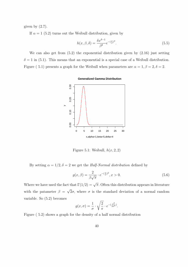
If α = 1 (5.2) turns out the Weibull distribution, given by
h(x, β, δ) =δxδ−1
βδe−( x
β)δ . (5.5)
We can also get from (5.2) the exponential distribution given by (2.16) just setting
δ = 1 in (5.1). This means that an exponential is a special case of a Weibull distribution.
Figure ( 5.1) presents a graph for the Weibull when parameters are α = 1, β = 2, δ = 2.
0 5 10 15 20 25 30
0.00
0.10
0.20
0.30
Generalized Gamma Distribution
x,alpha=1,beta=5,delta=4
y
Figure 5.1: Weibull, h(x, 2, 2)
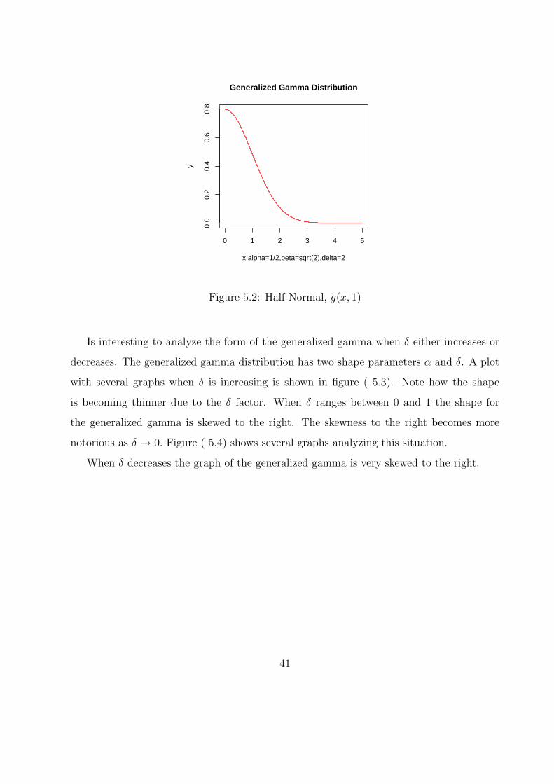
By setting α = 1/2, δ = 2 we get the Half-Normal distribution defined by
g(x, β) =2
β√π· e−( x
β)2 , x > 0. (5.6)
Where we have used the fact that Γ(1/2) =√π. Often this distribution appears in literature
with the patameter β =√2σ, where σ is the standard deviation of a normal random
variable. So (5.2) becomes
g(x, σ) =1
σ·√
2
π· e−( x2
2σ2 ).
Figure ( 5.2) shows a graph for the density of a half normal distribution
40
0 1 2 3 4 5
0.0
0.2
0.4
0.6
0.8
Generalized Gamma Distribution
x,alpha=1/2,beta=sqrt(2),delta=2
y
Figure 5.2: Half Normal, g(x, 1)
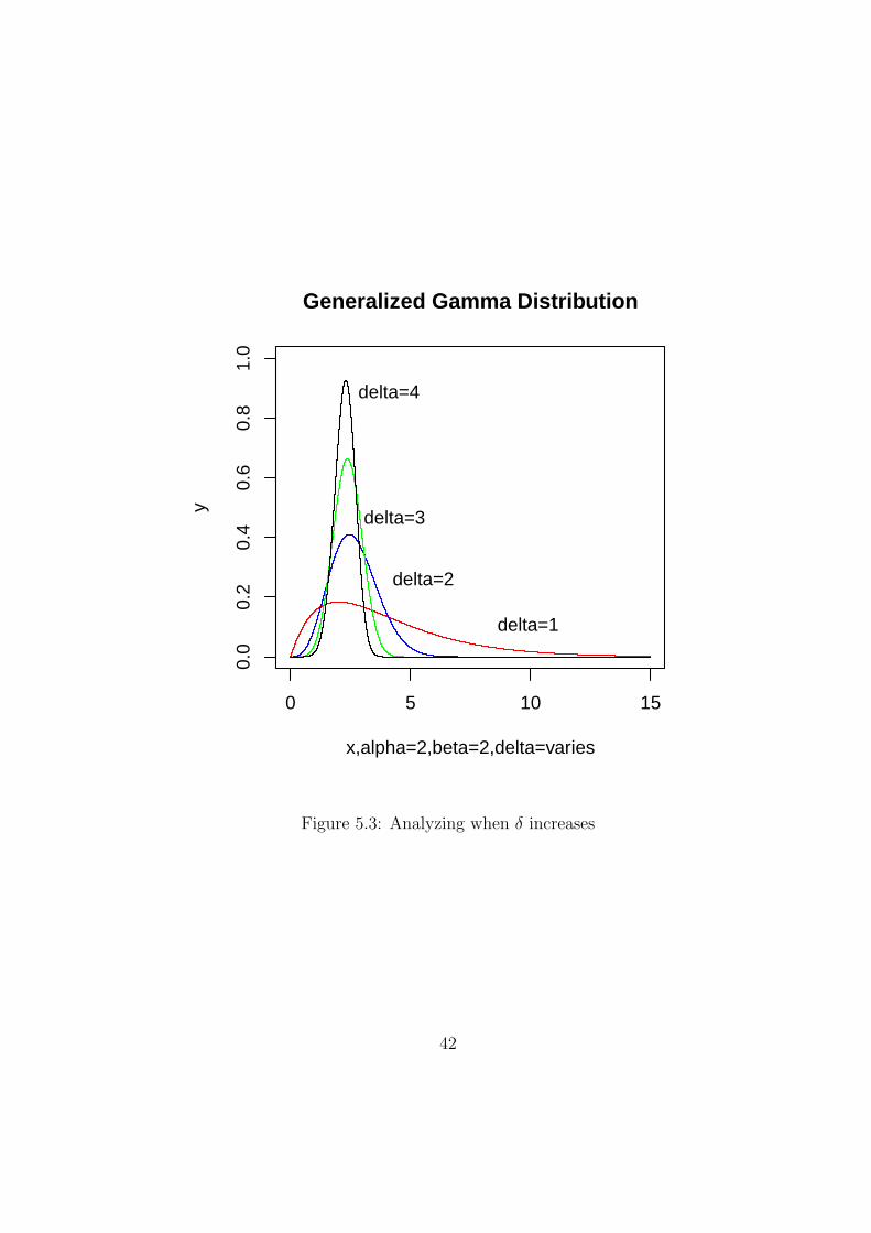
Is interesting to analyze the form of the generalized gamma when δ either increases or
decreases. The generalized gamma distribution has two shape parameters α and δ. A plot
with several graphs when δ is increasing is shown in figure ( 5.3). Note how the shape
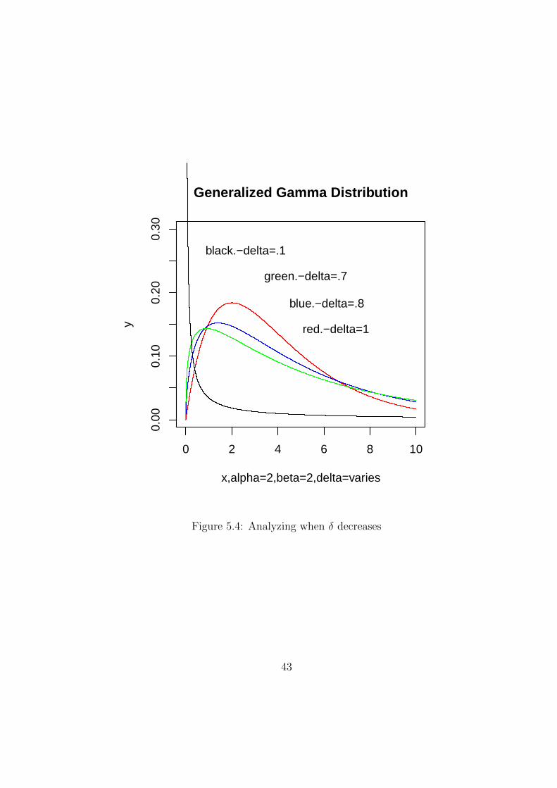
is becoming thinner due to the δ factor. When δ ranges between 0 and 1 the shape for
the generalized gamma is skewed to the right. The skewness to the right becomes more
notorious as δ → 0. Figure ( 5.4) shows several graphs analyzing this situation.
When δ decreases the graph of the generalized gamma is very skewed to the right.
41
0 5 10 15
0.0
0.2
0.4
0.6
0.8
1.0
Generalized Gamma Distribution
x,alpha=2,beta=2,delta=varies
y
delta=1
delta=2
delta=3
delta=4
Figure 5.3: Analyzing when δ increases
42
0 2 4 6 8 10
0.00
0.10
0.20
0.30
Generalized Gamma Distribution
x,alpha=2,beta=2,delta=varies
y red.−delta=1
blue.−delta=.8
green.−delta=.7
black.−delta=.1
Figure 5.4: Analyzing when δ decreases
43
Chapter 6
Estimation of parameters
6.1 Method of moments
To find the moments of the generalized gamma we again use a change of variable for the
equation ∫∞
0
xrf(x)dx =
∫∞
0
cxδα+r−1e−(x/β)δdx, (6.1)
and doing as before the change of variable y = (x/β)δ we get
δ
Γ(α)βδαδβr+δα−1β
∫∞
0
yα+rδ−1e−ydy.
So that the rth moment is given by
µ′
r =βrΓ(α + r
δ)
Γ(α). (6.2)
Thus the equations are obtained by equating population and sample moments
x =βΓ(α + 1
δ)
Γ(α)(6.3)
n∑
i=1
x2in
=β2Γ(α+ 2
δ)
Γ(α)(6.4)
n∑
i=1
x3in
=β3Γ(α + 3
δ)
Γ(α). (6.5)
Stacy ([16] 1965) suggested another method involving the method of moments. If we
set
Zi = ln(Xi/β)δ = δ(ln(Xi)− ln(β)), (6.6)
44
where the Xis, i = 1, . . . n, are independent generalized gamma random variables. And if
we denote the central moment of any random variable, say Z by µk(Z), k = 2, 3 . . . . So
that (6.6) indicates that
µk(Zi) = δkµk(ln(Xi)). (6.7)
Applying (5.3) and (5.4) to Z = ln(X/β)δ we see that
Z = ln(W ) = exp(αz − exp(z))/Γ(α), (6.8)
from where we get that the moment generating function of Z is
E(eθZ) = Γ(α+ θ)/Γ(α). (6.9)
It happens that any kth order derivative of Γ(α + θ), evaluated at θ = 0, is the same
whether the derivative is taken with respect to θ or α. Hence the kth moment of Z is
E(Zk) = Γ(k)(α)/Γ(α), (6.10)
where Γ(k)(α) is the kth derivative of Γ(α) with respect to α. It follows from (6.6) and (6.7)
that
δE(ln(X)− ln(β)) = µ, (6.11)
δ2µ2(ln(X)) = µ′,
δ3µ3(ln(X)) = µ′′.
In terms of the xi, yi = ln(xi), i = 1, 2, . . . n. Solutions for this equations are
a0 = exp(y − µ0/δ0) = exp(y − syµ0/(µ′
0)1/2),
δ0 = (µ′
0)1/2/sy,
−|gy| = µ′′/(µ′)3/2,
where β0 is determined by the last equation , β0 = µ(β0) and µ′
0 = µ′(β0). The sign of δ is
according to whether gy is less than or greater than zero respectively. Here y, s2y and gy are
respectively the sample mean, sample variance and sample skewness for the yi.
45
6.2 Maximum likelihood estimation
The likelihood function for the generalized gamma is given by
L(x1, . . . xn, α, β, δ) =n∏
i=1
f(xi, α, β, δ) =δn
Γ(α)n · βnαδ(x1, . . . xn)
δα−1e−∑n
i=1(xi/β)δ
. (6.12)
Taking natural log we have
L(x1 . . . xn, α, β, δ) = n ln(δ)−n ln(Γ(α))−nδα ln(β)+(αδ−1) ln(x1, . . . xn)−Σni=1(xi/β)
δ.
(6.13)
Now taking derivative the corresponding equations are
∂L
∂α= −nΓ
′(α)
Γ(α)− δn ln(β) + δ
n∑
i=1
ln(xi) = 0.
This can be expressed as
∂L
∂α= −nΓ
′(α)
Γ(α)+ δ
n∑
i=1
(ln(xi)− ln(β)
)= 0
= −nΓ′(α)
Γ(α)+ δ
n∑
i=1
ln(xi/β).
(6.14)
Differentiating with respect to β
∂L
∂β= −−δnα
β−
n∑
i=1
xδi (−δ)β−δ−1 =δ
β[−nα +
n∑
i=1
ln(xi/β)δ] = −nα +
n∑
i=1
ln(xi/β)δ = 0.
And from this last equation β turns out to be
β(α, δ) =(∑n
i=1(xi)δ)1/δ
(nα)1/δ(6.15)
it depends on α and from δ.
Differentiating with respect to δ
∂L
∂δ=n
δ− nα ln(β) + α
n∑
i=1
ln(xi)−n∑
i=1
((xi/β)
δ) · ln(xiβ)).
Now considering −n ln(β) = −∑n
i=1 ln(β) and using the properties of the function ln we
haven
δ+ α
n∑
i=1
ln(xiβ)−
n∑
i=1
(xiβ
)δln(xiβ
). (6.16)
46
So putting the value of β (6.15) into (6.16) we have
n
δ+ α
n∑
i=1
ln(xi
(∑n
i=1(xi)δ)1/δ
(nα)1/δ
)−n∑
i=1
( xi(∑n
i=1(xi)δ)1/δ
(nα)1/δ
)δln( xi(∑n
i=1(xi)δ)1/δ
(nα)1/δ
).
After rearranging terms we get an expression fot α in terms of δ :
α(δ) =1
δ ·[(∑n
i=1 ln(xi)/n)−(∑n
i=1 zδi ln(xi)
)/(∑n
i=1 xδi
)] . (6.17)
If we substitute (6.17) and (6.15) into (6.14) we will have an equation in terms of δ
only. This equation is
H(δ) = −ψ(α) + δ
∑ni=1 ln(xi)
n− ln
( n∑
i=1
xδi)+ ln(nα), (6.18)
where ψ(α) = Γ′(α)Γ(α)
is the digamma function. And α is given by (6.17).
Thus if we are going to try to estimate the parameters for the generalized gamma
distribution we need to solve (6.18) for δ. It is not always possible to find a solution for
H(δ). In many cases it is not even possible to know if there exists a solution. Some authors
say that the MLE may not exist unless n > 400. ([1] Continuous Univariate Distributions)
47
Chapter 7
Product and Ratio of two
Generalized Gamma
The problem of obtaining an explicit expression, without involving any unsolved integrals,
for both the probability density functon and the cumulative distribution of the product of
two independent random variables with generalized gamma distributions is a challenging
one. Expressions for the pdf of such a product had been obtained by some statisticians
in terms of complicated functions. But these functions are not readily computable. They
are usually computed in terms of the integrals that define them. And is even harder
try to extend beyond the product of more of two variables. The computations get really
complicated.
If
f(x1) =δ1
Γ(α1)βδ1α11
xδ1α1−11 e
−(x1β1
)δ1,
and
f(x2) =δ2
Γ(α2)βδ2α22
xδ2α2−12 e
−(x2β2
)δ2,
are two densities of two independent random variables X1 and X2 with generalized gamma
distribution then the joint density is given by
f(x1, x2) =δ1
Γ(α1)βδ1α11
xδ1α1−11 e
−(x1β1
)δ1 · δ2
Γ(α2)βδ2α22
xδ2α2−12 e
−(x2β2
)δ2. (7.1)
We want to find the distribution of Y = X1/X2. If we set W = X1 then we have the
variables
W = X1, and X2 =W
Y.
48
The jacobian for these transformations is given by w/y2. So the joint density of Y and W
is
fY,W (w, y) =δ1
Γ(α1)βδ1α11
· δ2
Γ(α2)βδ2α22
wδ1α1−1e−( w
β1)δ1(w/y)δ2α2−1e
−((w/y)β2
)δ2 · wy2
=
c1c2wδ1α1+δ2α2−2+1 · (1
y)δ2α2−1+2 · e−( w
β1)δ1e−(w/(yβ2))δ2 =
c1c2wδ1α1+δ2α2−1 · (1
y)δ2α2+1 · e−( w
β1)δ1e−(w/(yβ2))δ2 .
(7.2)
Thus
fY (y) =
∫∞
0
c1c2wδ1α1+δ2α2−1 · (1
y)δ2α2+1 · e−( w
β1)δ1e−(w/(yβ2))δ2dw
c1c2(1
y)δ2α2+1
∫∞
0
wδ1α1+δ2α2−1 · e−( wβ1
)δ1e−(w/(yβ2))δ2dw = (assume δ = δ1 = δ2)
c1c2(1
y)δ2α2+1
∫∞
0
wδ(α1+α2)−1 · e−( wβ1
)δe−(w/(yβ2))δdw =
c1c2(1
y)δ2α2+1
∫∞
0
wδ(α1+α2)−1 · e−wδ(
1
(β1)δ +
1
(yβ2)δ
)dw =
c1c2(1
y)δ2α2+1
∫∞
0
wδ(α1+α2)−1 · e−wδ/(β1/δ)δdw = where1
β=
( 1
(β1)δ+
1
(yβ2)δ)
c1c21
yδα2+1· β
α1+α2Γ(α1 + α2)
δ= c1c2
1
yδα2+1
(β1β2y)δ(α1+α2)
((yβ2)δ + (β1)δ)α1+α2Γ(α1 + α2) =
c1c2 · (β1β2)δ(α1+α2)Γ(α1 + α2)
δ
yδα1+δα2−δα2−1
((yβ2)δ + (β1)δ)α1+α2=
c1c2 · (β1β2)δ(α1+α2)Γ(α1 + α2)
δ
yδα1−1
((yβ2)δ + (β1)δ)α1+α2
= c1c2 · (β1β2
)δ(α1+α2) · Γ(α1 + α2)
δ
yδα1−1
(yδ + (β1
β2)δ)α1+α2
.
We will say that a random variable which has this distribution has a GGR (generalized
gamma ratio) with parameters (δ, k, α1, α2) where k = β1/β2.
Coelho and Mexia ([7] Coelho and Joao 2007) gave explicit and concise expressions for
the pdf and cumulative distributions of
W =m∏
j=1
Xj
49
where the Xj are independent random variables with all distinct shape parameters. If
Xj ∼ GGR(kj, α1j, α2j, δj), j = 1 . . .m. Where all the parameters are positive. Let
s1j = αij and s2j = α2j,
then if δjs1j 6= δks1k and δjs2j 6= δks2k, for all j 6= k, j, k = 1, 2 . . . n, the density and
cumulative distribution of the random variable
W =m∏
j=1
Xj, (7.3)
are given by
fW (w) =
limn→∞K1K2
∑mj=1
∑nh=0H2jhdhj(w/K
∗)s∗1jh 1
wif 0 < w ≤ K∗
limn→∞K1K2
∑mj=1
∑nh=0H1jhchj(w/K
∗)−s∗2jh 1w
if w ≥ K∗,
And
FW (w) =
limn→∞K1K2
∑mj=1
∑nh=0H2jh
dhjs∗1jh
(w/K∗)s∗1jh if 0 < w ≤ K∗
limn→∞K1K2
∑mj=1
∑nh=0
{H2jh
dhjs∗1jh
+H1jhchjs∗2jh
(1− ( w
K∗ )−s2jh
)}if w ≥ K∗,
,
where
K∗ =m∏
j=1
k−1/δjj ,
K1 =m∏
j=1
n∏
h=0
s∗1jh, K2 =m∏
j=1
n∏
h=0
s∗2jh,
and, for j = 1. . . . ,m and n = 0, 1, . . . ,
chj =m∏
η=1
n∏
ν=
1
s∗2ην − s∗2jh, chj =
m∏
η=1
n∏
ν=
1
s∗1ην − s∗1jh,
and
H1jh =m∑
k=1
n∑
l=0
dkls∗2jh + s∗1kl
, H2jh =m∑
k=1
n∑
l=0
ckls∗1jh + s∗2kl
,
with
s∗1jh = δ∗j (s1j + h) and s∗2jh = δ∗j (s2j + h), (j = 1, . . .m).
There are other considerations when the parameters are not the same. (See [7] Coelho
and Joao 2007).
50
Chapter 8
Hierarchical Models
All of the cases seen thus far a random variable had a single distribution depending on
parameters. Sometimes is more convenient to think of the things in a hierarchy. A well
known hierarchical model is the following. An insect lays a large number of eggs , each
surviving with probability p. On the average, how many eggs will survive? The ”large
number” of eggs laid is a random variable , often chosen to be Poisson (λ). Furthermore
we assume that each eggs survival is independent, then we have Bernoulli trials. So if we
set X = number of survivors and Y = number of Bernoulli trials we have
X|Y ∼ binomial(Y, p)
Y ∼ Poisson(λ).
We want to compute
P (X = x) =∞∑
y=0
P (X = x, Y = y)
=∞∑
y=0
P (X = x|Y = y)P (Y = y)
=∞∑
y=0
[(yx)px(1− p)y−x][e−λλy
y!].
Since X|Y = y is binomial(y, p) and Y is Poisson(λ). If we now simplify this last expression
51
we have
P (X = x) =(λpe−λ)
x!
∞∑
y=x
((1− p)λ)y−x
(y − x)!
=(λpe−λ)
x!
∞∑
y=x
((1− p)λ)t
(t)!
=(λpe−λ)
x!e(1−p)λ
=(λpe−λ)
x!e−λp,
so X ∼Poisson(λp) And from this is easily seen that
EX = λp.
Now if X is a random variable with Generalized Gamma density in the form of (5.2)
we will use the notation X ∼ GG(α, β, δ). We will also write c(α, β, δ) = δβδαΓ(α)
to refer
to the constant in the generalized gamma density. Let’s consider Y |Λ ∼ Poisson(Λ) and
Λ ∼ Gg(α, β, δ). Then the distribution of Y is given by
f(y) =
∫∞
0
λye−y
y!· c(α, β, δ) · λα−1 · e−(λ
β)δdλ.
To evaluate this integral we wiil use the fact that e−x =∑
∞
k=0(−1)k
k!xk. So for this case we
have
f(y) =
∫∞
0
λye−λ
y!· c(α, β, δ) · λα−1 ·
∞∑
k=0
(−1)k
k!
(λβ
)δkdλ
=c(α, β, δ)
y!
∫∞
0
e−λλy+α−1 ·∞∑
k=0
(−1)k
k!
(λβ
)δkdλ
=c(α, β, δ)
y!
∞∑
k=0
∫∞
0
(−1)k
k!
(λβ
)δk · λy+α−1 · e−λdλ
=c(α, β, δ)
y!
∞∑
k=0
(−1)k
k!βk
∫∞
0
λδk+y+α−1 · e−λdλ.
Seeing the integral in the right hand side as Γ(δk + y + α) we get
f(y) =c(α, β, δ)
y!
∞∑
k=0
(−1)k
k!βk· Γ(δk + y + α). (8.1)
52
So we can get the distribution of Y just by changing parameters. For example if δ = β = 1
we have that Λ is a random variable with standard gamma density, so
f(y) =c(α, 1, 1)
y!·
∞∑
k=0
(−1)k
k!Γ(k + y + α) =
1
Γ(α)y!·
∞∑
k=0
(−1)k
k!Γ(k + y + α).
If α = δ = 1 we have an exponential distribution. So (8.1) becomes
f(y) =1
βy!·
∞∑
k=0
(−1)k
βkk!Γ(k + y + 1)
=1
βy!·
∞∑
k=0
(−1)k
βkk!
∫∞
0
λk+ye−λdλ
=1
βy!
∫∞
0
∞∑
k=0
(−1)k
βkk!· λkλy · e−λdλ
=1
βy!
∫∞
0
∞∑
k=0
(−1)k
k!
(λβ
)k · λy · e−λdλ
=1
βy!
∫∞
0
eλβ · e−λ · λydλ =
1
βy!
∫∞
0
e−(1+ 1
β
)λ · λydλ.
Now making the change of variable u = (1 + 1β)λ we arrive to
f(y) =1
β · y!
∫∞
0
e−u · uy
(1 + 1β)y
· β
β + 1du
=1
(1 + 1β)y · (β + 1) · y!
∫∞
0
e−uuydu
=Γ(y + 1)
(1 + 1β)y · (β + 1) · y! =
1
(1 + 1β)y · (β + 1)
.
Remember that for any two random variables we can relate them with the following
formula
E(X) = E(E(X|Y )), (8.2)
and
V ar(X) = E(V ar(X|Y )) + V ar(E(X|Y )), (8.3)
provided that the expectations exist. For the same case from above we have that
E(Y ) = E(E(Y |Λ)) = E(Λ) =βΓ(α + 1
δ)
Γ(α),
53
which is just the expected value given by (6.3).
The variance for Y is given by
V ar(Y ) = E(V ar(Y |Λ)) + V ar(E(Y |Λ))
= E(Λ) + V ar(Λ) = E(Λ) + E(Λ2)− (E(Λ))2
=βΓ(α+ 1
δ)
Γ(α)+β2Γ(α + 2
δ)
Γ(α)+β2Γ(α+ 1
δ)2
Γ(α)2.
54
Chapter 9
Random Numbers Generation for a
Generalized Gamma Distribution
If we set the change of variable y = (x/β)δ in (5.2) a standard gamma distribution with
parameter α is obtained.
f(x, α, β, δ)dx =δ
βδαΓ(α)· xδα−1e−( x
β)δ
=δ
βδαΓ(α)· (βy1/δ)δα−1e−(βy
1/δ
β)δ · βy
1−δδ
δ( because dx =
βy1−δδ
δ)
=1
Γ(α)· yα−1/δ+1/δ−1 · e−y
= f(y) =1
Γ(α)· yα−1e−y.
So we can generate random numbers for y (which is easy with the adequate software)
in this gamma density and then relate this numbers to the generalized gamma by means
of the equation
x = βy1/δ. (9.1)
This can work to estimate the cummulative distribution when X ∼ GG(α, β, δ). That is,
for any t > 0
P (X ≤ t) =
∫ t
0
δ
βδαΓ(α)· xδα−1e−( x
β)δdx. (9.2)
If we generate n random numbers x1, x2, . . . xn fromX, t > 0 then the empirical distribution
is defined as
Fn(x) =n∑
i=1
1{xi ≤ t}. (9.3)
55
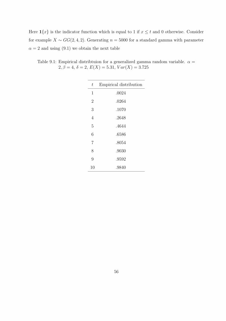
Here 1{x} is the indicator function which is equal to 1 if x ≤ t and 0 otherwise. Consider
for example X ∼ GG(2, 4, 2). Generating n = 5000 for a standard gamma with parameter
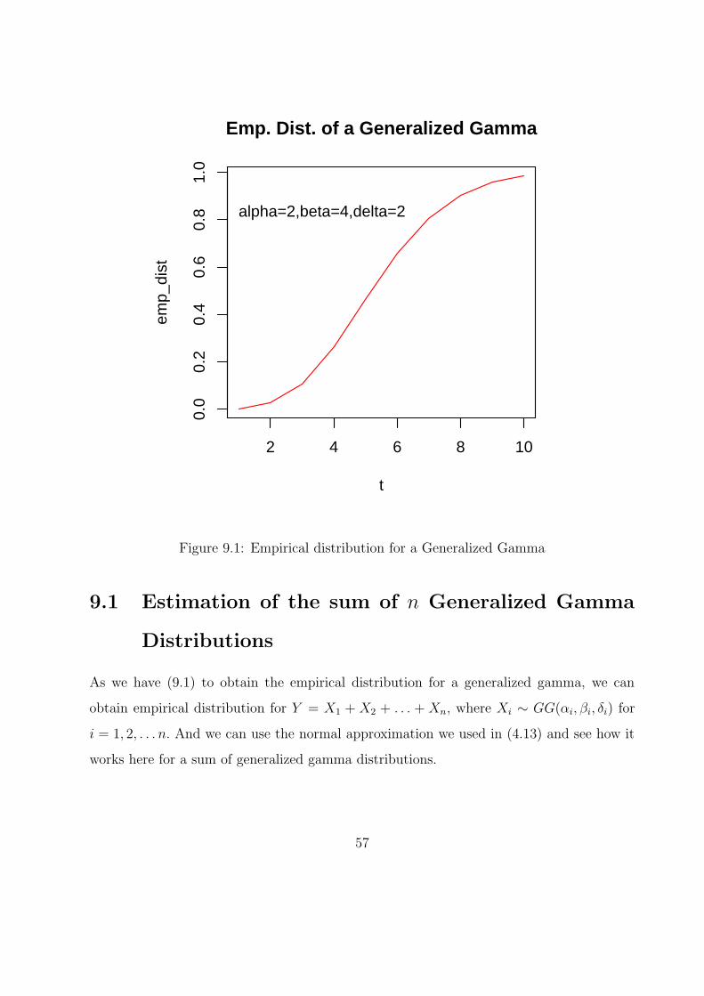
α = 2 and using (9.1) we obtain the next table
Table 9.1: Empirical distribtuion for a generalized gamma random variable. α =2, β = 4, δ = 2, E(X) = 5.31, V ar(X) = 3.725
t Empirical distribution
1 .0024
2 .0264
3 .1070
4 .2648
5 .4644
6 .6586
7 .8054
8 .9030
9 .9592
10 .9840
56
2 4 6 8 10
0.0
0.2
0.4
0.6
0.8
1.0
Emp. Dist. of a Generalized Gamma
t
emp_
dist
alpha=2,beta=4,delta=2
Figure 9.1: Empirical distribution for a Generalized Gamma
9.1 Estimation of the sum of n Generalized Gamma
Distributions
As we have (9.1) to obtain the empirical distribution for a generalized gamma, we can
obtain empirical distribution for Y = X1 + X2 + . . . + Xn, where Xi ∼ GG(αi, βi, δi) for
i = 1, 2, . . . n. And we can use the normal approximation we used in (4.13) and see how it
works here for a sum of generalized gamma distributions.
57
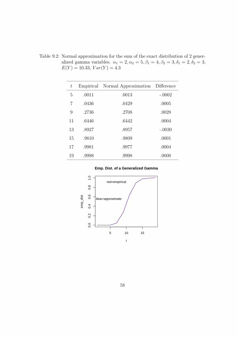
Table 9.2: Normal approximation for the sum of the exact distribution of 2 gener-alized gamma variables. α1 = 2, α2 = 5, β1 = 4, β2 = 3, δ1 = 2, δ2 = 3,E(Y ) = 10.33, V ar(Y ) = 4.3
t Empirical Normal Approximation Difference
5 .0011 .0013 -.0002
7 .0436 .0429 .0005
9 .2736 .2708 .0028
11 .6446 .6442 .0004
13 .8927 .8957 -.0030
15 .9810 .9809 .0001
17 .9981 .9977 .0004
19 .9998 .9998 .0000
5 10 15
0.0
0.2
0.4
0.6
0.8
1.0
Emp. Dist. of a Generalized Gamma
t
emp_
dist
red=empirical
blue=approximate
58
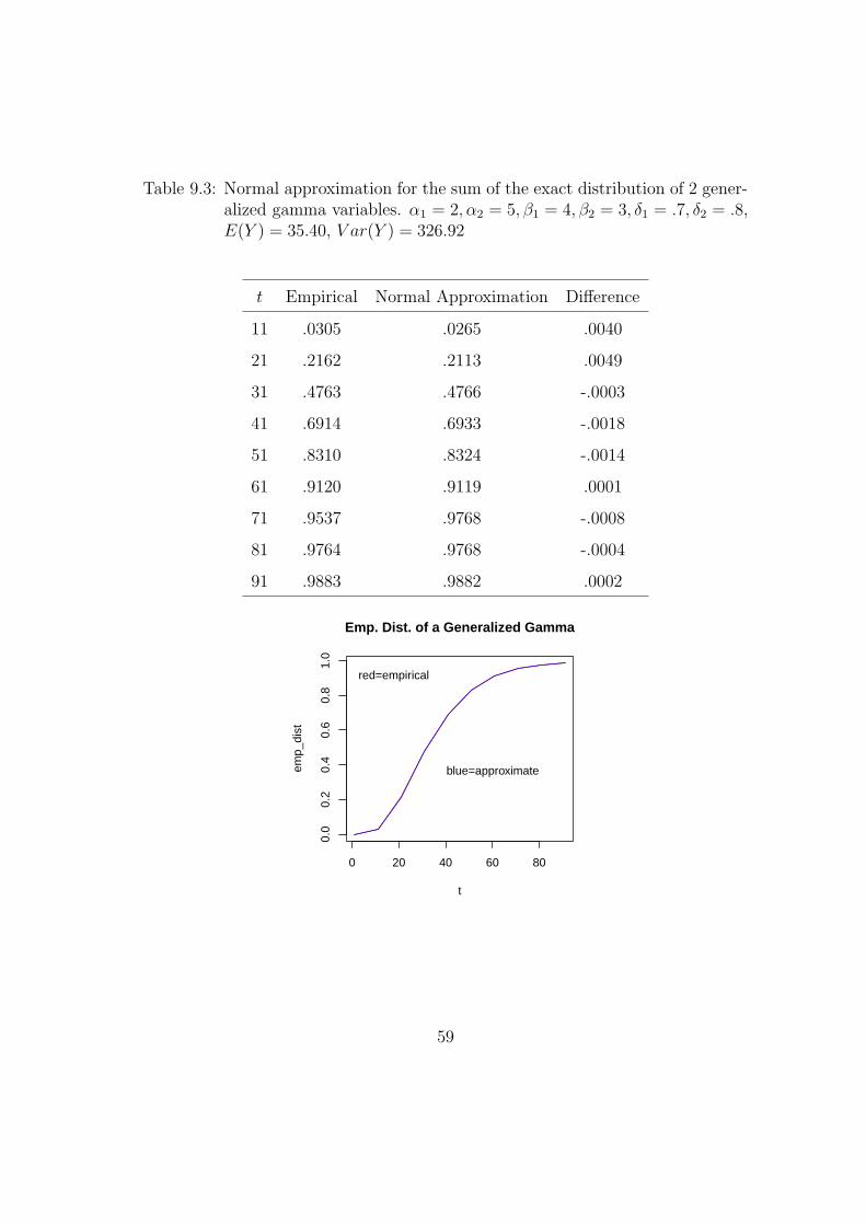
Table 9.3: Normal approximation for the sum of the exact distribution of 2 gener-alized gamma variables. α1 = 2, α2 = 5, β1 = 4, β2 = 3, δ1 = .7, δ2 = .8,E(Y ) = 35.40, V ar(Y ) = 326.92
t Empirical Normal Approximation Difference
11 .0305 .0265 .0040
21 .2162 .2113 .0049
31 .4763 .4766 -.0003
41 .6914 .6933 -.0018
51 .8310 .8324 -.0014
61 .9120 .9119 .0001
71 .9537 .9768 -.0008
81 .9764 .9768 -.0004
91 .9883 .9882 .0002
0 20 40 60 80
0.0
0.2
0.4
0.6
0.8
1.0
Emp. Dist. of a Generalized Gamma
t
emp_
dist
red=empirical
blue=approximate
59
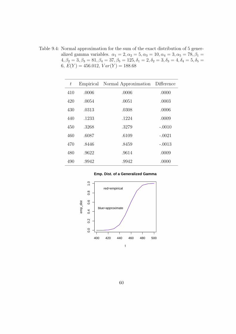
Table 9.4: Normal approximation for the sum of the exact distribution of 5 gener-alized gamma variables. α1 = 2, α2 = 5, α3 = 10, α4 = 3, α5 = 78, β1 =4, β2 = 3, β3 = 81, β4 = 37, β5 = 125, δ1 = 2, δ2 = 3, δ3 = 4, δ4 = 5, δ5 =6, E(Y ) = 456.012, V ar(Y ) = 188.68
t Empirical Normal Approximation Difference
410 .0006 .0006 .0000
420 .0054 .0051 .0003
430 .0313 .0308 .0006
440 .1233 .1224 .0009
450 .3268 .3279 -.0010
460 .6087 .6109 -.0021
470 .8446 .8459 -.0013
480 .9622 .9614 .0009
490 .9942 .9942 .0000
400 420 440 460 480 500
0.0
0.2
0.4
0.6
0.8
1.0
Emp. Dist. of a Generalized Gamma
t
emp_
dist
red=empirical
blue=approximate
60
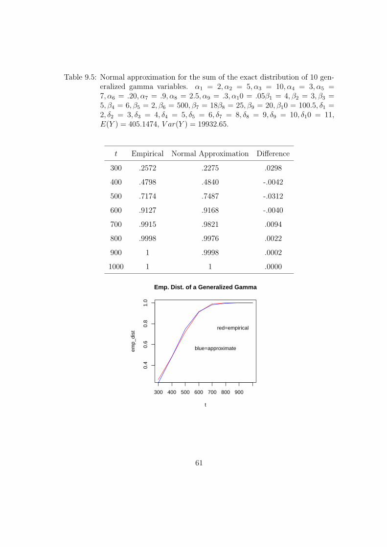
Table 9.5: Normal approximation for the sum of the exact distribution of 10 gen-eralized gamma variables. α1 = 2, α2 = 5, α3 = 10, α4 = 3, α5 =7, α6 = .20, α7 = .9, α8 = 2.5, α9 = .3, α10 = .05β1 = 4, β2 = 3, β3 =5, β4 = 6, β5 = 2, β6 = 500, β7 = 18β8 = 25, β9 = 20, β10 = 100.5, δ1 =2, δ2 = 3, δ3 = 4, δ4 = 5, δ5 = 6, δ7 = 8, δ8 = 9, δ9 = 10, δ10 = 11,E(Y ) = 405.1474, V ar(Y ) = 19932.65.
t Empirical Normal Approximation Difference
300 .2572 .2275 .0298
400 .4798 .4840 -.0042
500 .7174 .7487 -.0312
600 .9127 .9168 -.0040
700 .9915 .9821 .0094
800 .9998 .9976 .0022
900 1 .9998 .0002
1000 1 1 .0000
300 400 500 600 700 800 900
0.4
0.6
0.8
1.0
Emp. Dist. of a Generalized Gamma
t
emp_
dist
red=empirical
blue=approximate
61
References
[1] Continuous Univariate Distributions, 1994, Norman L. Johnson, Samuel Kotz, N. Bal-
akrishnan, Second edition, Vol. 1 Wiley Series in Probability and Mathematical Statis-
tics.
[2] Amorosol, (1925). Ricerche intorno alla curva dei redditi. Ann. Mat. Pura Appl. Ser.
4 21 123-159
[3] D’Addario, R. (1932). Intorno alla curva dei redditi di Amoroso. Riv. Italiana Statist.
Econ. Fnanza, anno 4, No. 1
[4] Van B. Parr,J.T. Webster, A method for discriminating between Failure Density Func-
tions Used in Reliability Predictions,Technometrics, Vol 7. No. 1 (Feb. 1965), pp 1-10
[5] S. C. Choi and R. Wette, (1969) Maximum Likelihood Estimation of the Parameters
of the Gamma Distribution and Their Bias, Technometrics, 11(4) 683690
[6] P.C Consul and G. C. Jain, Statistische Theorie,On the Log-Gamma Distribution and
its Properties
[7] Carlos A. Coelho and Joao t. Mexia, (2007), On the Distribution of Product and Ratio
of Independent Generalized Gamma-Ratio, The Indian Journal of Statistics (2003-),
Vol. 69, No.2 pp 221-255.
[8] John E. Freunds, Mathematical Statistics with Applications, Seventh Edition, Pearson
Prentice Hall (2004), Upper Saddle River, New Jersey 221-255.
[9] P.G. Moschopoulos, (1985) The Distribution of the sum of Independent Gamma Ran-
dom Variables, Annals of the Institute of Statistical Mathematics, 37, Part A, 541-544
62
[10] P.G. Moschopoulos, W.B. Canada (1984) The distribution function of a linear com-
bination of Chi-squares, Comps and Maths with applications, Vol 10. No. 4/5 pp.
383-386
[11] P.G. Moschopoulos,(1983) On a new Transformation to Normality, Communication
Statistics-Theory and Methods, 12(16), pp. 1873-1878
[12] P.G. Moschopoulos, Govind, S. Mudholkar, (1983) A Likelihood Ratio Based Normal
Approximation for the Non-Null Distribution of the Multiple Correlation Coefficient,
Communication Statistics-Simulations and Computations, 12(3), pp 355-371
[13] Pham-Gia, Turkkan, N. (2002). Operations on the generalized-F variables and appli-
cations. Statistics, 36, 195-209.
[14] Roberts,C.D. (1971). On the distribution of random variables whose mth absolute
power is gamma, Sankhya, Series A, 33, pp. 229-232
[15] E.W. Stacy, (1962) A generalization of the gamma distribution. The Annals of Math-
ematical Statistics, Vol. 33, No. 3, pp. 1187-1192
[16] E.W. Stacy and G. A. Mihram. (1965) Estimation for a generalized gamma distribu-
tion, Technometrics, Vol 7 No.3 pp.349-358
[17] Stacy E. W. Mihram G.A. (1965). Parameter estimation for a generalized gamma
distribution, Technometrics, 7, pp. 349-358.
[18] D.R. Jensen and Herbert Solomon (1972) A Gaussian Approximation to the Distribu-
tion of a Definite Quadratic Form, JASA, Vol.67. No. 340, pp 898-902.
63
Chapter 10
Appendix
All the codes have been written in the software R.
10.1 Code to Approximate the sum of k Independent
Gamma Random Variables
#Number of terms
n=10
#Number of generation for the random numbers
n2=1000
#Setting the parameters
alpha=c(1:n)
beta=c(1:n)
alpha[1]=2
alpha[2]=2.5
alpha[3]=3
alpha[4]=3.5
alpha[5]=4
alpha[6]=4.5
64

alpha[7]=5
alpha[8]=5.5
alpha[9]=6
alpha[10]=6.5
beta[1]=2
beta[2]=2.5
beta[3]=3
beta[4]=3.5
beta[5]=4
beta[6]=4.5
beta[7]=5
beta[8]=5.5
beta[9]=6
beta[10]=6.5
#Normal approx
k1=sum(alpha*beta)
k2=sum(alpha*beta^2)
k3=sum(alpha*beta^3)
phi_2=k2/k1
phi_3=k3/k1
phi_4=k4/k1
65

h=1-k1*k3/(3*k2^2)
mu_h=1+h*(h-1)*phi_2/(2*k1)+h*(h-1)*(h-2)*(4*phi_3+3*(h-3)*phi_2^2)/(24*k1^2)
sigma_h=phi_2*h^2/(k1)+(h-1)*h^(2)*(2*phi_3+(3*h-5)*phi_2^2)/(2*k1^2)
#Estimation with random numbers
Gen=matrix(0,n,n2)
for(i in 1:n)
{
Gen[i,]=rgamma(n2,alpha[i],1/beta[i])
}
#Estimation of alpha
alpha_est=c(1:n)
s_est=c(1:n)
for(i in 1:n)
{
s_est[i]=log(mean(Gen[i,])) -sum(log(Gen[i,]))/n2
alpha_est[i]=(3-s_est[i]+sqrt((s_est[i]-3)^2
+24*s_est[i]))/(12*s_est[i])
}
#Estimation of the parameter "beta"
beta_est=c(1:n)
for(i in 1:n)
{
beta_est[i]=mean(Gen[i,])/(alpha_est[i])
66

}
beta_est
alpha_est
#Exact distribution
#Number of terms we will use in the infinite sum
k=100
#Length of the subintervals the interval is divided in
c=.1
#Right extreme of the interval
lim_r=300
#Setting the minimum between beta’s
beta_min=min(beta)
#Setting the coefficient rho
rho=sum(alpha)
#Coefficients C and Lower gamma
beta_min_ov_beta=(beta_min^{rho})/(prod(beta^{alpha}))
C=prod(beta_min_ov_beta)
G=1-beta_min/beta
lower_gamma_matrix=matrix(1,n,(k+1))
for(j in 1:n)
67
{
for(i in 1:(k+1))
{
lower_gamma_matrix[j,i]=(alpha[j]*(G[j])^{i})/i
}
}
lower_gamma=colSums(lower_gamma_matrix)
#Setting the delta’s
delta=c(1:(k+1))
delta[1]=lower_gamma[1]
for(j in 2:(k+1))
{
b=c(1:(j-1))
for(v in 1:(j-1)){b[v]=v*lower_gamma[v]*delta[(j-v)]}
d=sum(b)+j*lower_gamma[j]
delta[j]=(1/j)*(d)
}
#Domain
y=seq(0,lim_r,by=c)
#Density
density_sum_gamma=matrix(1,(k+1),(1/(c/lim_r))+1)
for(u in 1:(k+1))
{
density_sum_gamma[u,]=((gamma(rho+u)*(beta_min)^{rho+u})^{-1})
*delta[u]*y^{rho+u-1}*exp(-y/beta_min)
}
68

E=C*colSums(density_sum_gamma)+C*y^{rho-1}*exp(-y/beta_min)
*((gamma(rho)*(beta_min)^{rho})^{-1})
#Approximate
expect_z=sum(alpha*beta)
var_z=sum(alpha*beta^{2})
beta_z=var_z/expect_z
alpha_z=expect_z^(2)/var_z
App=1/(beta_z^{alpha_z}*gamma(alpha_z))*y^{alpha_z-1}*exp(-y/beta_z)
#Graphs for the distribution
#Exact
pgamma_vector_ex=c(1:lim_r)
for(j in 1:lim_r)
{
A=c(1:(k+1))
for(i in 1:(k+1))
{
A[i]=delta[i]*pgamma(j,rho+i,1/beta_min)
}
distribution_1=c(A,pgamma(j,rho,1/beta_min))
pgamma_vector_ex[j]=C*sum(distribution_1)
}
domain=c(1:lim_r)
Ex=pgamma_vector_ex
69

#Approximate
pgamma_vector_app=c(1:lim_r)
for(j in 1:lim_r)
{
pgamma_vector_app[j]=pgamma(j,alpha_z,1/beta_z,)
}
App=pgamma_vector_app
#Estimated
pgamma_vector_est=c(1:lim_r)
for(j in 1:lim_r)
{
pgamma_vector_est[j]=pgamma(j,alpha_z_est,1/beta_z_est)
}
Est=pgamma_vector_est
#Estimated_h
k1=sum(alpha*beta)
k2=sum(alpha*beta^2)
k3=2*sum(alpha*beta^3)
phi_2=k2/k1
phi_3=k3/k1
phi_4=k4/k1
h=1-k1*k3/(3*k2^2)
70

#h=1/3
mu_h=1+h*(h-1)*phi_2/(2*k1)+h*(h-1)*(h-2)*(4*phi_3+3*(h-3)*phi_2^2)/(24*k1^2)
sigma_h=phi_2*h^2/(k1)+(h-1)*h^(2)*(2*phi_3+(3*h-5)*phi_2^2)/(2*k1^2)
pgamma_vector_est_h=c(1:lim_r)
for(j in 1:lim_r)
{
z_h=((j/k1)^{h} -mu_h)/(sqrt(sigma_h))
pgamma_vector_est_h[j]=pnorm(z_h)
}
Est_h=pgamma_vector_est_h
par(mfrow=c(1,2))
plot(domain,Ex,type="l",col="red",xlab="x",main="Exact distribution")
#plot(domain,App,type="l",col="blue",xlab="x",main="Two moments app")
plot(domain,Est_h,type="l",col="brown",xlab="x",main="Normal Approx")
#plot(domain,Ex_est,type="l",col="black")
#plot(domain,Est,type="l",col="green")
#Distribution several times
#Approximate
a_1=180
b_1=340
c_1=20
vector_t=seq(a_1,b_1,by=c_1)
Approx_1=c(1:((b_1-a_1)/c_1 +1))
for(i in 1:((b_1-a_1)/c_1+(1)))
{
71
Approx_1[i]=pgamma(vector_t[i]/beta_z,alpha_z)
}
#Exact_dist=C*sum(distribution)
#Exact
Exact_1=c(1:((b_1-a_1)/c_1 +1))
for(j in 1:((b_1-a_1)/c_1+(1)))
{
A=c(1:(k+1))
for(i in 1:(k+1))
{
A[i]=delta[i]*pgamma(vector_t[j],rho+i,1/beta_min,)
}
distribution_2=c(A,pgamma(vector_t[j],rho,1/beta_min))
Exact_1[j]=C*sum(distribution_2)
}
#Estimated exact
Exact_1_est=c(1:((b_1-a_1)/c_1 +1))
for(j in 1:((b_1-a_1)/c_1+(1)))
{
A_est=c(1:(k+1))
for(i in 1:(k+1))
{
A_est[i]=delta_est[i]*pgamma(vector_t[j],rho_est+i,1/beta_min_est)
}
distribution_2_est=c(A_est,pgamma(vector_t[j],rho_est,1/beta_min_est,))
72
Exact_1_est[j]=C_est*sum(distribution_2_est)
}
#Estimated with two moments
Estimated_1=c(1:((b_1-a_1)/c_1 +1))
for(i in 1:((b_1-a_1)/c_1+(1)))
{
Estimated_1[i]=pgamma(vector_t[i],alpha_z_est,1/beta_z_est)
}
#Estimated with h
Normal_App_1=c(1:((b_1-a_1)/c_1 +1))
z_h=c(1:((b_1-a_1)/c_1 +1))
for(i in 1:((b_1-a_1)/c_1+(1)))
{
z_h[i]=((vector_t[i]/k1)^{h} -mu_h)/(sqrt(sigma_h))
Normal_App_1[i]=pnorm(z_h[i])
}
Approx=round(Approx_1,digits=7)
Exact=round(Exact_1,digits=7)
Estimated=round(Estimated_1,digits=7)
Est_ex=round(Exact_1_est,digits=7)
Normal_App=round(Normal_App_1,digits=7)
Diff_1=Exact_1-Approx_1
Diff_E_A=round(Diff_1,digits=7)
Diff_10_3_1=Diff*1000
Diff_10_3=round(Diff_10_3_1)
Diff_2=Exact-Estimated
73

Diff_E_Est=round(Diff_2,digits=7)
Diff_3=Exact-Est_ex
Diff_E_EE=round(Diff_3,digits=7)
Diff_4=Exact_1-Normal_App_1
Diff_E_Normal=round(Diff_4,digits=7)
#Printing out results
#Table_results=cbind(vector_t,Exact,Approx,Est_ex,Estimated,Normal_App,
Diff_E_A,Diff_E_EE,Diff_E_Est,Diff_E_Normal)
#Table_results=cbind(vector_t,Exact,Approx,Diff_E_A)
#Table_results=cbind(vector_t,Exact,Est_ex,Diff_E_EE)
Table_results=cbind(vector_t,Exact,Normal_App,Diff_E_Normal)
#Table_results=cbind(vector_t,Exact_1,Approx_1,
Estimated_h_1,Diff_1,Diff_4)
Table=data.frame(Table_results)
#write.table(Table,"C:/Users/Hugo/Desktop/Hugo/Thesis/
Simulation_Independent_Sum_of_Gamma/ex_norm_tabla_1.txt",sep=",")
74
10.2 Code to Approximate the Sum of k Independent
Generalized Gamma Random Variables
#Sum of Generalized Gamma
#Empirical distribution
#Number of terms
n=5
#Number of random data generated
n1=50000
#Standard gamma numbers
y_ran_data=matrix(0,n,n1)
#Parameters
alpha=c(1:n)
beta=c(1:n)
delta=c(1:n)
alpha[1]=2
alpha[2]=5
alpha[3]=10
alpha[4]=3
alpha[5]=78
#alpha[6]=.2
#alpha[7]=.9
#alpha[8]=2.5
#alpha[9]=.3
75

#alpha[10]=.05
beta[1]=4
beta[2]=3
beta[3]=81
beta[4]=37
beta[5]=125
#beta[6]=500
#beta[7]=18
#beta[8]=25
#beta[9]=20
#beta[10]=100
#m=2
delta[1]=.5
delta[2]=.6
delta[3]=.3
delta[4]=.8
delta[5]=.2
#delta[6]=m+5
#delta[7]=m+6
#delta[8]=m+7
#delta[9]=m+8
#delta[10]=m+9
#Gen gamma numbers
x_vectors=matrix(0,n,n1)
for(i in 1:n)
76
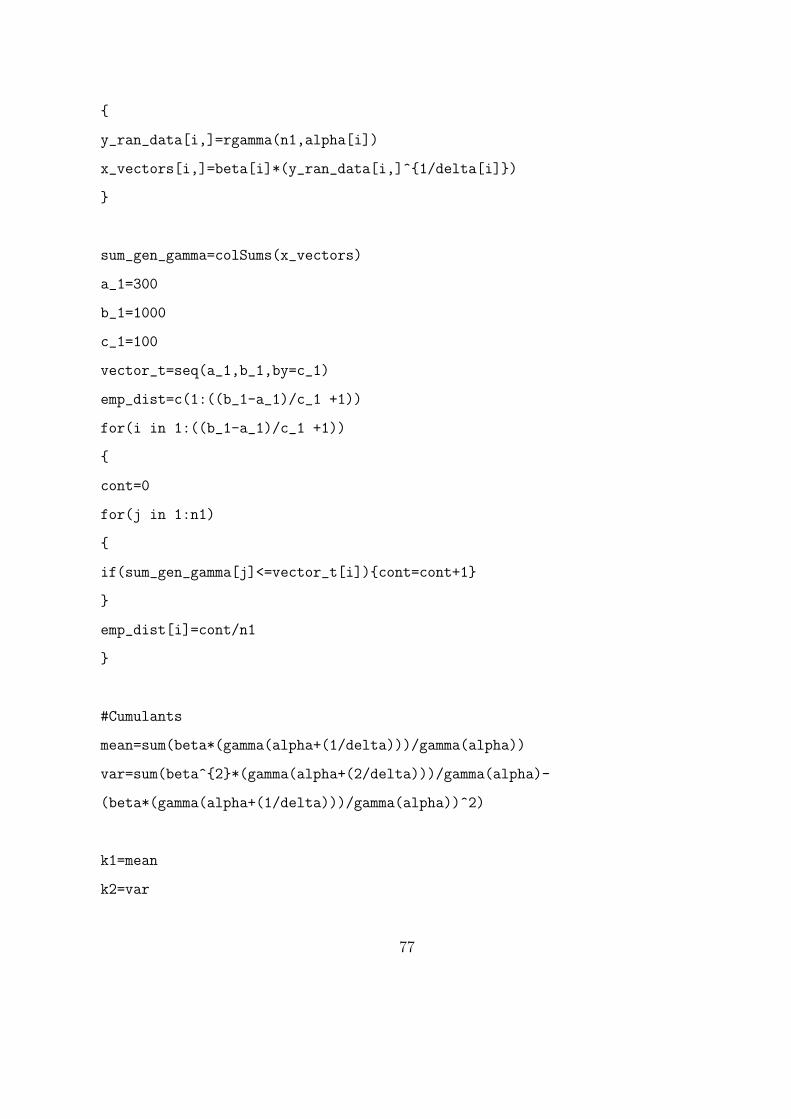
{
y_ran_data[i,]=rgamma(n1,alpha[i])
x_vectors[i,]=beta[i]*(y_ran_data[i,]^{1/delta[i]})
}
sum_gen_gamma=colSums(x_vectors)
a_1=300
b_1=1000
c_1=100
vector_t=seq(a_1,b_1,by=c_1)
emp_dist=c(1:((b_1-a_1)/c_1 +1))
for(i in 1:((b_1-a_1)/c_1 +1))
{
cont=0
for(j in 1:n1)
{
if(sum_gen_gamma[j]<=vector_t[i]){cont=cont+1}
}
emp_dist[i]=cont/n1
}
#Cumulants
mean=sum(beta*(gamma(alpha+(1/delta)))/gamma(alpha))
var=sum(beta^{2}*(gamma(alpha+(2/delta)))/gamma(alpha)-
(beta*(gamma(alpha+(1/delta)))/gamma(alpha))^2)
k1=mean
k2=var
77

k3=sum(beta^{3}*gamma(alpha+(3/delta))/(gamma(alpha))-3*beta^{2}
*(gamma(alpha+(2/delta)))/gamma(alpha)
*(beta*(gamma(alpha+(1/delta)))/gamma(alpha))+2*(beta*(gamma(alpha+(1/delta)))
/gamma(alpha))^(3))
phi_2=k2/k1
phi_3=k3/k1
phi_4=k4/k1
h=1-k1*k3/(3*k2^2)
mu_h=1+h*(h-1)*phi_2/(2*k1)+h*(h-1)*(h-2)*(4*phi_3+3*(h-3)*phi_2^2)/(24*k1^2)
sigma_h=phi_2*h^2/(k1)+(h-1)*h^(2)*(2*phi_3+(3*h-5)*phi_2^2)/(2*k1^2)
Normal_App_sum_gg=c(1:((b_1-a_1)/c_1 +1))
z_h=c(1:((b_1-a_1)/c_1 +1))
for(i in 1:((b_1-a_1)/c_1+(1)))
{
z_h[i]=((vector_t[i]/k1)^{h} -mu_h)/(sqrt(sigma_h))
Normal_App_sum_gg[i]=pnorm(z_h[i])
}
diff=emp_dist-Normal_App_sum_gg
results=cbind(vector_t,emp_dist,round(Normal_App_sum_gg,4),round(diff,4))
#results=cbind(vector_t,emp_dist)
Results=data.frame(results)
#write.table(Results,"C:/Users/Hugo/Desktop/Hugo/Thesis
/Simulation_Independent_Sum_of_Gamma/sum_gen_gamm_7.txt",sep=",")
78

Results
plot(vector_t,emp_dist,type="l",col="red",xlab="t",main
="Emp. Dist. of a Generalized Gamma")
lines(vector_t,Normal_App_sum_gg,col="blue")
text(locator(1),"red=empirical")
text(locator(1),"blue=approximate")
79
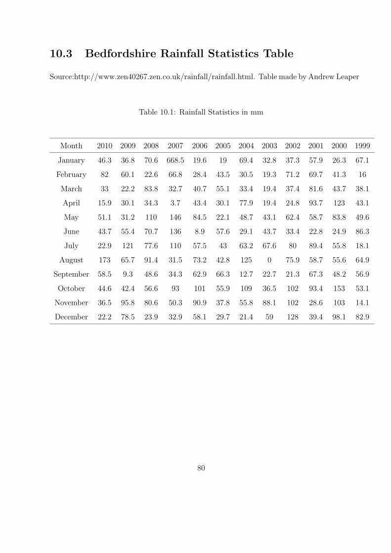
10.3 Bedfordshire Rainfall Statistics Table
Source:http://www.zen40267.zen.co.uk/rainfall/rainfall.html. Table made by Andrew Leaper
Table 10.1: Rainfall Statistics in mm
Month 2010 2009 2008 2007 2006 2005 2004 2003 2002 2001 2000 1999
January 46.3 36.8 70.6 668.5 19.6 19 69.4 32.8 37.3 57.9 26.3 67.1
February 82 60.1 22.6 66.8 28.4 43.5 30.5 19.3 71.2 69.7 41.3 16
March 33 22.2 83.8 32.7 40.7 55.1 33.4 19.4 37.4 81.6 43.7 38.1
April 15.9 30.1 34.3 3.7 43.4 30.1 77.9 19.4 24.8 93.7 123 43.1
May 51.1 31.2 110 146 84.5 22.1 48.7 43.1 62.4 58.7 83.8 49.6
June 43.7 55.4 70.7 136 8.9 57.6 29.1 43.7 33.4 22.8 24.9 86.3
July 22.9 121 77.6 110 57.5 43 63.2 67.6 80 89.4 55.8 18.1
August 173 65.7 91.4 31.5 73.2 42.8 125 0 75.9 58.7 55.6 64.9
September 58.5 9.3 48.6 34.3 62.9 66.3 12.7 22.7 21.3 67.3 48.2 56.9
October 44.6 42.4 56.6 93 101 55.9 109 36.5 102 93.4 153 53.1
November 36.5 95.8 80.6 50.3 90.9 37.8 55.8 88.1 102 28.6 103 14.1
December 22.2 78.5 23.9 32.9 58.1 29.7 21.4 59 128 39.4 98.1 82.9
80
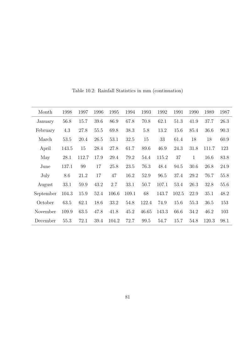
Table 10.2: Rainfall Statistics in mm (continuation)
Month 1998 1997 1996 1995 1994 1993 1992 1991 1990 1989 1987
January 56.8 15.7 39.6 86.9 67.8 70.8 62.1 51.3 41.9 37.7 26.3
February 4.3 27.8 55.5 69.8 38.3 5.8 13.2 15.6 85.4 36.6 90.3
March 53.5 20.4 26.5 53.1 32.5 15 33 61.4 18 18 60.9
April 143.5 15 28.4 27.8 61.7 89.6 46.9 24.3 31.8 111.7 123
May 28.1 112.7 17.9 29.4 79.2 54.4 115.2 37 1 16.6 83.8
June 137.1 99 17 25.8 23.5 76.3 48.4 94.5 30.6 26.8 24.9
July 8.6 21.2 17 47 16.2 52.9 96.5 37.4 29.2 76.7 55.8
August 33.1 59.9 43.2 2.7 33.1 50.7 107.1 53.4 26.3 32.8 55.6
September 104.3 15.9 52.4 106.6 109.1 68 143.7 102.5 22.9 35.1 48.2
October 63.5 62.1 18.6 33.2 54.8 122.4 74.9 15.6 55.3 36.5 153
November 109.9 63.5 47.8 41.8 45.2 46.65 143.3 66.6 34.2 46.2 103
December 55.3 72.1 39.4 104.2 72.7 99.5 54.7 15.7 54.8 120.3 98.1
81
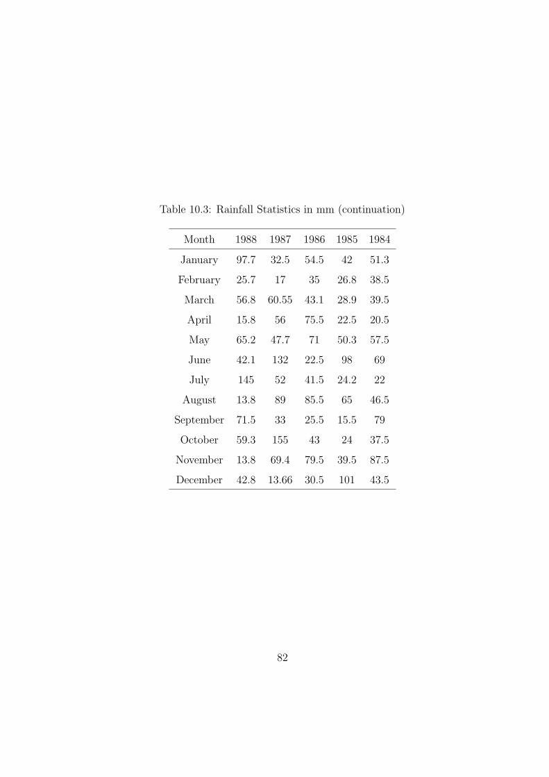
Table 10.3: Rainfall Statistics in mm (continuation)
Month 1988 1987 1986 1985 1984
January 97.7 32.5 54.5 42 51.3
February 25.7 17 35 26.8 38.5
March 56.8 60.55 43.1 28.9 39.5
April 15.8 56 75.5 22.5 20.5
May 65.2 47.7 71 50.3 57.5
June 42.1 132 22.5 98 69
July 145 52 41.5 24.2 22
August 13.8 89 85.5 65 46.5
September 71.5 33 25.5 15.5 79
October 59.3 155 43 24 37.5
November 13.8 69.4 79.5 39.5 87.5
December 42.8 13.66 30.5 101 43.5
82
Curriculum Vitae
Vıctor Hugo Jimenez Nava was born on May 8, 1984. The second son of Jorge Sabino
Jimenez and Marıa Elva Nava Morales, he graduated from Juarez Autonomous University,
Juarez, Chihuahua Mexico, in the spring of 2009. He obtained a bachelor in mathematics.
He has attended research summer programs in Mexico. He went to Colima, Colima at
the Colima Autonomous University in 2007 and Guanajuato, Guanajuato, at the Research
Center in Mathematics in 2008. He entered University of Texas at El Paso in the fall of
2009. While pursuing a master’s degree in statistics he worked as a Teaching Assistant, and
as instructor for two mathematical courses directed to freshman students. He submitted
this work on december 2011 as a part of the requirements to complete his master in statistics
at the University of Texas at El Paso.
83
Recommended