American Institute of Aeronautics and Astronautics
1
Further Development of Verification Check-cases for Six-Degree-of-Freedom Flight Vehicle Simulations
E. Bruce Jackson* and Michael M. Madden† NASA Langley Research Center, Hampton, VA 23681, USA
Dr. Robert Shelton‡ and Dr. A. A. Jackson§ NASA Johnson Space Center, Houston, TX 77058, USA
Manuel P. Castro** and Deleena M. Noble** NASA Armstrong Flight Research Center, Edwards, CA 93523, USA
Curtis J. Zimmerman†† NASA Marshall Space Flight Center, Huntsville, AL 35812, USA
Jeremy D. Shidner‡‡, Joseph P. White§§, Soumyo Dutta***, Eric M. Queen***, Richard W. Powell‡‡, William A. Sellers†††, Scott A. Striepe‡‡‡, and John Aguirre§§§ NASA Langley Research Center, Hampton, VA 23681, USA
Nghia Vuong****, Scott E. Reardon††††, Michael J. Weinstein†††† and William Chung‡‡‡‡ NASA Ames Research Center, Mountain View, CA 94035, USA
and
Jon S. Berndt§§§§ JSBSim Open Source Project, Westminster, CO 80027, USA
This follow-on paper describes the principal methods of implementing, and documents the results of exercising, a set of six-degree-of-freedom rigid-body equations of motion and planetary geodetic, gravitation and atmospheric models for simple vehicles in a variety of endo- and exo-atmospheric conditions with various NASA, and one popular open-source, engineering simulation tools. This effort is intended to provide an additional means of verification of flight simulations. The models used in this comparison, as well as the resulting time-history trajectory data, are available electronically for persons and organizations wishing to compare their flight simulation implementations of the same models.
* Sr. Aerospace Engineer, Dynamic Systems and Control Branch, MS 308, AIAA Associate Fellow. † Chief Scientist, Simulation Development and Analysis Branch, MS 125B, AIAA Senior Member. ‡ Lead, JSC Engineering Orbital Dynamics (JEOD), Engineering Directorate, Mail Code ER7. § Sr. Engineer, Jacobs Engineering Group, Inc., Engineering Directorate, AIAA Associate Fellow. ** Aerospace Engineer, AFRC Simulation Engineering, MS 4840. †† Aerospace Engineer, Guidance, Navigation and Mission Analysis Branch, MSFC/EV42, AIAA Member. ‡‡ Aerospace Engineer, Analytical Mechanics & Assoc., MS 489, Associate Fellow (Powell); Sr. Member (Shidner). §§ Senior Project Engineer, Analytical Mechanics & Associates, MS 489. *** Aerospace Engineer, Atmos. Flight & Entry Systems Branch, MS 489, Sr. Member (Queen), Member (Dutta). ††† Senior Systems Analyst, Stinger Gha arin Technologies, Inc., MS 489, AIAA Member. ‡‡‡ Aerospace Engineer, Atmospheric Flight & Entry Systems Branch, MS 489. §§§ Scientific Programmer, Analytical Mechanics & Associates, MS 489. **** Systems Software Engineer, Aerospace Sim. Research & Development Branch, MS 243-5, AIAA Member. †††† Flight Simulation Engineer, Aerospace Sim. Research & Development Branch, MS 243-5, AIAA Member. ‡‡‡‡ Sr. Simulation Engineer, SAIC, Aerospace Sim. Res. & Devel. Branch, MS-243-6, Associate Fellow. §§§§ Project Lead, Member.
https://ntrs.nasa.gov/search.jsp?R=20150006038 2018-05-02T11:13:50+00:00Z
American Institute of Aeronautics and Astronautics
2
I. Nomenclature CD = Aerodynamic drag coefficient F = Force h = Geometric altitude J2 = Second degree zonal harmonic coefficient of gravitation R = Radius to center of Earth T = Torque t = Time x = Body longitudinal axis, +forward y = Body lateral axis, +right to an observer facing in positive x direction Z = Geopotential height z = Body vertical axis, +down Acronymns 6-DOF = Six-degree-of-freedom CM = Center of Mass CSV = Comma-Separated Values DAVE-ML = Dynamic Aerospace Vehicle Exchange Markup Language DOF = Degrees-of-freedom ECEF = Earth-centered, earth-fixed (rotating coordinate frame) ECI = Earth-centered inertial (non-rotating coordinate frame) EOM = Equations of Motion GEM-T1 = Goddard Earth Model T1 ISS = International Space Station J2000 = Earth-centered inertial frame for epoch 2000 JEOD = JSC Engineering Orbital Dynamics JSBSim = Open-source, data-driven, simulation framework in C++ kt = knots (nautical miles per hour) LaSRS++ = Langley Standard Real-time Simulation in C++ LVLH = Local Vertical, Local Horizontal frame MAVERIC = Marshall Aerospace Vehicle Representation in C MET = Marshall Engineering Thermosphere MRC = Moment Reference Center NED = North-East-Down NESC = NASA Engineering and Safety Center POST II = Program to Optimize Simulated Trajectories II S-119 = ANSI/AIAA S-119-2011 Flight Dynamic Model Exchange Standard Unicode = Uniform character encoding standard URL = Uniform Resource Locator VMSRTE = Vertical Motion Simulator Real-Time Environment WGS-84 = World Geodetic System 1984 XML = eXtensible Markup Language
I. Introduction HE rise of innovative unmanned aeronautical systems and the emergence of commercial space activities have resulted in a number of relatively new aerospace organizations that are designing innovative systems and
solutions. These organizations use a variety of commercial off-the-shelf and in-house-developed simulation and analysis tools including 6-degree-of-freedom (6-DOF) flight simulation tools. The increased affordability of computing capability has made high-fidelity flight simulation practical for all participants. Verification of the tools’ equations-of-motion and environment models (e.g., atmosphere, gravitation, and geodesy) is desirable to assure accuracy of results. However, aside from simple textbook examples, minimal verification data exists in open literature for 6-DOF flight simulation problems.
This paper compares multiple solution trajectories to a set of verification check-cases that covered atmospheric and exo-atmospheric (i.e., orbital) flight. Each scenario consisted of pre-defined flight vehicles, initial conditions,
T
American Institute of Aeronautics and Astronautics
3
and maneuvers. These scenarios were implemented and executed in a variety of analytical and real-time simulation tools. This tool-set included simulation tools in a variety of programming languages based on modified flat-Earth, round-Earth, and rotating oblate spheroidal Earth geodesy and gravitation models, and independently derived equations-of-motion and propagation techniques. The resulting simulated parameter trajectories were compared by over-plotting and difference-plotting to yield a family of solutions.
In total, seven simulation tools were exercised. Participating in this exercise were participants from NASA Ames Research Center (ARC), Armstrong Flight Research Center (AFRC), Johnson Space Center (JSC), Langley Research Center (LaRC), and Marshall Space Flight Center (MSFC), and an open-source simulation tool development project (i.e., JSBSim).
The vehicle models defined by the check-cases were published in the American Institute of Aeronautics and Astronautics/American National Standards Institute (AIAA/ANSI) S-119-2011 Flight Dynamics Model Exchange Standard (S-119) markup language1, making them realizable in a variety of proprietary and non-proprietary implementations. This set of models and the resulting trajectory plots from a collection of simulation tools may serve as a preliminary verification aide for organizations that are developing their own atmospheric and orbital simulation tools and frameworks. The models and trajectory data are available from the NASA Engineering and Safety Center’s (NESC) Academy website, in the Flight Mechanics area2. This exercise is believed to be the first publically available comparison of a set of 6-DOF flight simulation tools. An earlier NASA study4 compared exo-atmospheric scenarios between NASA and international space agency partners, but those results are not publically available.
An earlier paper reported on preliminary results of this effort that included mostly simple check-cases; this paper presents the final results of this multiyear effort involving additional, more complex, vehicle models and maneuvers. Models and data sets associated with this effort are available on-line for others to use for comparison with additional simulation tools.3
II. Approach The NESC’s Technical Fellow for Flight Mechanics assembled a team to develop flight simulation verification
data sets. This team mapped out an approach to developing check-cases for comparison and cross-verification purposes.
The team agreed that a set of scenarios involving simple models would be developed and simulated by each participant in their preferred simulation tool. In an attempt to build a “consensus” solution for 6-DOF flight vehicle simulations, a set of relatively simple flight vehicle models was developed, with a set of maneuvers from specified initial conditions, in a variety of atmospheric, gravitational, and geodetic configurations. It was anticipated the resulting trajectories would fall into one or more families of solutions based upon assumptions and simplifications (e.g., flat-Earth conditions). The basic parameters were agreed upon and further discussion led to the set of scenarios described in Section II.H. Formats for specifying the models, initial conditions, and resulting time-history data were agreed to and a plan for presenting the data was developed.
Instead of identifying a single “known good” simulation tool, or requiring that all “good” trajectories match within a predefined tolerance, the approach taken was to present comparison plots of the results of each simulation tools. If acceptable agreement between the parameter trajectories generated by the tools was found, then those trajectories could serve as a verification guide. If unacceptable difference in results was evident, then an attempt would be made to identify an assumption, design choice, and/or an implementation difference to explain the disparity, and the set of trajectories would serve as a family of possible solutions. (For this purpose, the term “acceptable agreement” remained a subjective concept.)
One of the overall objectives was to generate a publically available report containing the salient results for use by current and future organizations. Furthermore, it was desirable to make the vehicle models and resulting trajectory data available electronically for ease of comparison by developers of other simulation tools.
A. Check-Case Vehicle Models A set of reference flight vehicles was proposed, based primarily on existing non-proprietary vehicle models. For
the atmospheric scenarios, the “vehicles” included a spheroid (i.e., cannonball), a brick to evaluate rotational dynamics, a subsonic fighter with representative nonlinear aerodynamics, propulsion, and control law models, and a two-stage rocket. For the orbital cases, a larger spheroid, a cylindrical rocket body, and a simplified International Space Station (ISS) models were re-used from an earlier comparison study4.
American Institute of Aeronautics and Astronautics
4
B. Check-Case Geodesy Models One of the challenges in performing 6-DOF flight simulations is the choice in how to model the Earth’s shape
and motion. Early low-speed atmospheric flight simulations often used a flat-Earth approximation that was sufficient for recreating landing and takeoff dynamics. Early computational performance limitations made this simplifying approximation attractive for pilot-in-the-loop (“real-time”) training or research and development simulations.
As digital computers grew in capability, simulation of flight using more accurate spherical and oblate rotating Earth models became practical from a cost/time standpoint. Many atmospheric flight simulation tools incorporated the standard DoD World Geodetic System 1984 (WGS-84)5 ellipsoidal Earth model even though an iterative solver, or other multi-step iterative process, was normally required to convert between inertial coordinates and geodetic coordinates (i.e., latitude, longitude, and altitude) with the ellipsoidal geodesy model.
The atmospheric check-case scenarios developed for this study included round non-rotating, round rotating, and ellipsoidal rotating Earth models. The orbital check-case scenarios used the oblate WGS-84 model exclusively.
C. Check-Case Coordinate Systems A number of coordinate system definitions and transformations were required in this exercise including: J2000
inertial; Earth-centered inertial (ECI); Earth-centered Earth-fixed (ECEF) in either geocentric or geodetic frames; local-vertical, local-horizontal (LVLH); north-east-down (NED); launch site; and body coordinates.
D. Check-Case Gravitation Models In parallel with a choice of Earth geodesy models was a corresponding choice of gravitation models. The
simplest model had gravitational attraction varying inversely with the square of the vehicle distance from Earth’s center. This simplified model is often used with the approximation of a spherical Earth.
A more sophisticated gravitation model, including gravitational harmonics that vary with latitude and longitude, is normally employed for ellipsoidal Earth models. For atmospheric check-cases with a WGS-84 Earth, the first non-zero term of the harmonic series (i.e., J2 gravitation) is included. Orbital scenarios included the J2 and higher harmonic terms (i.e., to 8 × 8) using the Goddard Earth Model (GEM)-T1 harmonic coefficients6.
E. Check-Case Atmosphere Models US 1976. The US Standard 1976 Atmosphere model7 was used for the majority of the atmospheric check-case
scenarios. This model can be implemented as linear interpolation of the one-dimensional tables given in the source document with ambient pressure, temperature, and density as a function of geometric altitude (h) or geopotential height (Z). A more accurate implementation was to realize atmospheric properties directly from the non-linear numerical equations used to generate the tables published in reference 7.
Marshall Engineering Thermosphere (MET). The MET is appropriate for modeling the thermosphere region of the Earth’s atmosphere, located above the stratosphere (i.e., greater than 90 km) but below the exosphere (i.e., less than 500 km). MET is employed for most of the orbital check-cases. This model is not publicly available, but can be requested from the MSFC Natural Environments Branch.
F. Check-Case Data Formats The use of standard formats should significantly shorten the process of sharing models and comparing results.
While some setup was required for each tool to receive models in an unfamiliar format and translate the data in a locally-compatible format, it was hoped the ability to quickly implement model changes and generate new results would be enhanced by this investment.
Reference models. Most of the atmospheric check-cases vehicle models were specified using the format in Ref. 1 (i.e., S-119), which makes use of an extensible markup language (XML) based grammar, DAVE-ML8. This format attempted to encode the salient flight characteristics of an aerospace vehicle (i.e., aerodynamic and inertial properties) unambiguously in a text file that is human- and machine-readable, and with sufficient metadata to be easily converted into code and to be readily archivable. The most complex model attempted in this study was the single-engine F-16 aircraft defined in DAVE-ML using S-119 variable names that included an inertial/mass properties model, a non-linear aerodynamic model, and two separate control law subsystem models. These models are available from the NESC Academy website (Ref 2).
Time-History Data. Despite an attempt to identify a more efficient binary data format for the several million data points that were generated in this effort, the team eventually stored data in a comma-separated-values (.CSV) text format. These files used column headers to identify the values represented and rows to group values associated with regular time steps of simulation. The check-case files were large (e.g., 12 MB in one case) as a result of using
American Institute of Aeronautics and Astronautics
5
text instead of binary value representations, but this format was felt to be better suited for archival purposes and to be more readily accessible by other reviewers. The time-history data files are also available from the NESC Academy website (Ref. 2).
G. Participating Simulation Tools Developers of several NASA and one open-source simulation tools agreed to participate in this comparison on a
voluntary basis. The set of tools involved included simulations suited primarily for atmospheric flight, exo-atmospheric flight, and some were applicable to both flight regimes. Not all simulation tools attempted to execute every check-case. The team agreed to a ground rule that a minimum of three data sets (i.e., parameter trajectories) generated by independent tools were necessary to warrant inclusion in this exercise.
The assembled tool-set included: • Core from ARFC • JEOD from JSC • JSBSim (open source EOM) • LaSRS++ from LaRC • MAVERIC from MSFC • POST II from LaRC • VMSRTE from ARC The resulting data-sets cited later in this report are identified anonymously as resulting from “SIM 1” or “SIM
A”; this is intentional to encourage participation and comparison between tool providers.
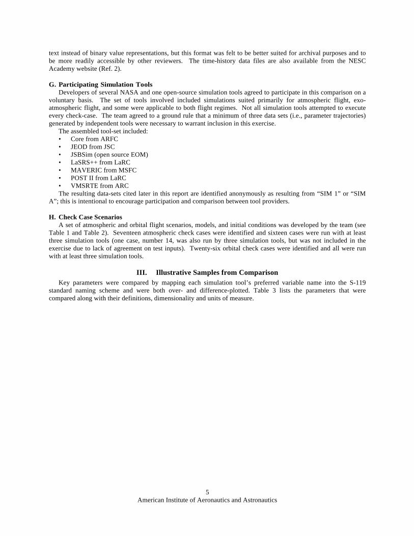
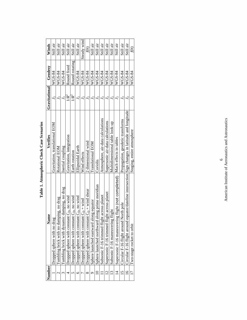
H. Check Case Scenarios A set of atmospheric and orbital flight scenarios, models, and initial conditions was developed by the team (see
Table 1 and Table 2). Seventeen atmospheric check cases were identified and sixteen cases were run with at least three simulation tools (one case, number 14, was also run by three simulation tools, but was not included in the exercise due to lack of agreement on test inputs). Twenty-six orbital check cases were identified and all were run with at least three simulation tools.
III. Illustrative Samples from Comparison Key parameters were compared by mapping each simulation tool’s preferred variable name into the S-119
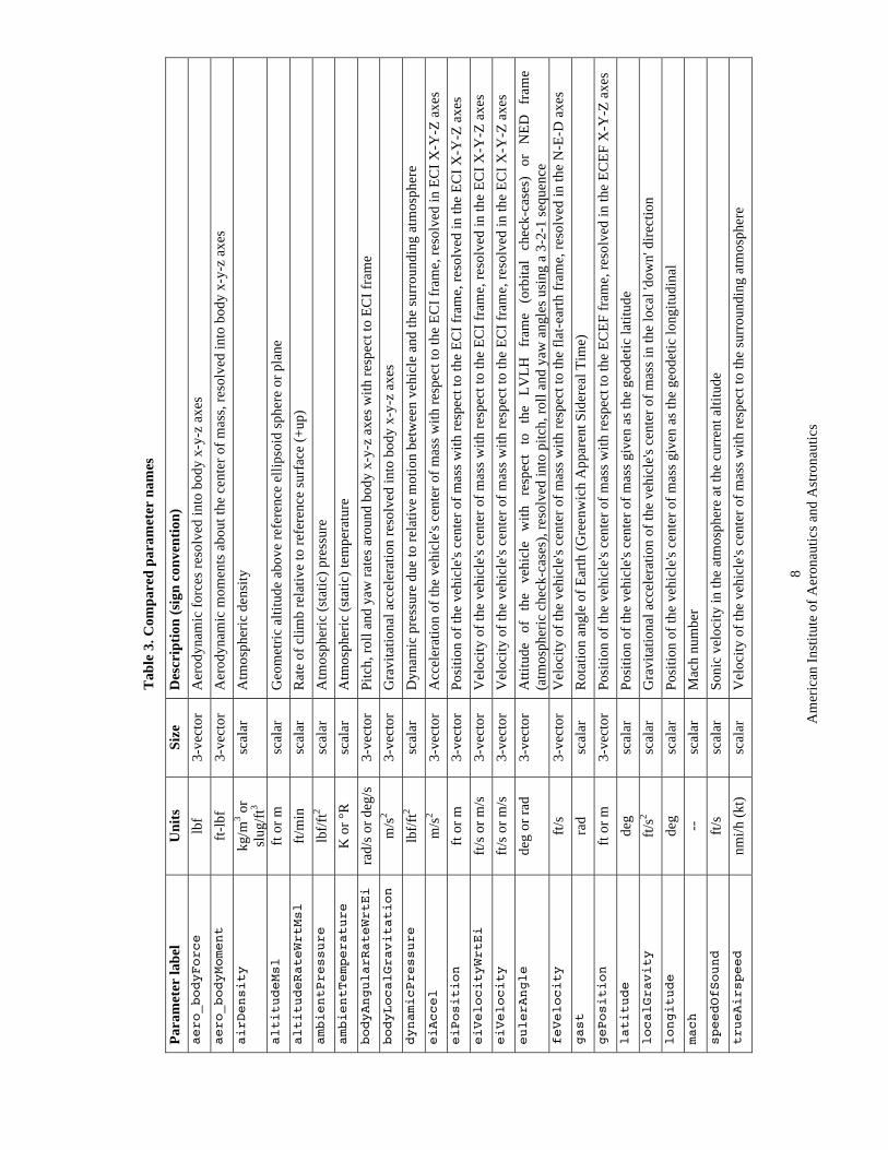
standard naming scheme and were both over- and difference-plotted. Table 3 lists the parameters that were compared along with their definitions, dimensionality and units of measure.
A
mer
ican
Inst
itute
of A
eron
autic
s and
Ast
rona
utic
s 6
Tab
le 1
. Atm
osph
eric
Che
ck C
ase
Scen
ario
s
Num
ber
Nam
e V
erifi
es
Gra
vita
tiona
l G
eode
sy
Win
ds
1 D
ropp
ed sp
here
with
no
drag
G
ravi
tatio
n, tr
ansl
atio
nal E
OM
J 2
W
GS-
84
Still
air
2 Tu
mbl
ing
bric
k w
ith n
o da
mpi
ng, n
o dr
ag
Rot
atio
nal E
OM
J 2
W
GS-
84
Still
air
3 Tu
mbl
ing
bric
k w
ith d
ynam
ic d
ampi
ng, n
o dr
ag
Iner
tial c
oupl
ing
J 2
WG
S-84
St
ill a
ir 4
Dro
pped
sphe
re w
ith c
onst
ant C
D, n
o w
ind
Gra
vita
tion,
inte
grat
ion
1/R2
Rou
nd fi
xed
Still
air
5 D
ropp
ed sp
here
with
con
stan
t CD, n
o w
ind
Earth
rota
tion
1/R2
Rou
nd ro
tatin
g St
ill a
ir 6
Dro
pped
sphe
re w
ith c
onst
ant C
D, n
o w
ind
Ellip
soid
al E
arth
J 2
W
GS-
84
Still
air
7 D
ropp
ed sp
here
with
con
stan
t CD +
win
d W
ind
effe
cts
J 2
WG
S-84
St
eady
win
d 8
Dro
pped
sphe
re w
ith c
onst
ant C
D +
win
d sh
ear
2 di
men
sion
al w
ind
J 2
WG
S-84
f(h
) 9
Sphe
re la
unch
ed e
astw
ard
alon
g eq
uato
r Tr
ansl
atio
nal E
OM
J 2
W
GS-
84
Still
air
10
Sphe
re la
unch
ed n
orth
war
d al
ong
prim
e m
erid
ian
Cor
iolis
J 2
W
GS-
84
Still
air
11
Subs
onic
F-1
6 tri
mm
ed fl
ight
acr
oss p
lane
t A
tmos
pher
e, a
ir-da
ta c
alcu
latio
ns
J 2
WG
S-84
St
ill a
ir 12
Su
pers
onic
F-1
6 tri
mm
ed fl
ight
acr
oss p
lane
t Su
pers
onic
air-
data
cal
cula
tions
J 2
W
GS-
84
Still
air
13
Subs
onic
F-1
6 m
aneu
verin
g fli
ght
Mul
tidim
ensi
onal
tabl
e lo
ok-u
p J 2
W
GS-
84
Still
air
14
Supe
rson
ic F
-16
man
euve
ring
fligh
t ()
Mac
h ef
fect
s in
tabl
es
J 2
WG
S-84
St
ill a
ir 15
C
ircul
ar F
-16
fligh
t aro
und
Nor
th p
ole
Prop
agat
ion,
geo
detic
tran
sfor
ms
J 2
WG
S-84
St
ill a
ir 16
C
ircul
ar F
-16
fligh
t aro
und
equa
tor/d
atel
ine
inte
rsec
tion
Sign
cha
nges
in la
titud
e an
d lo
ngitu
de
J 2
WG
S-84
St
ill a
ir 17
Tw
o-st
age
rock
et to
orb
it St
agin
g, e
ntire
atm
osph
ere
J 2
WG
S-84
f(h
)
A
mer
ican
Inst
itute
of A
eron
autic
s and
Ast
rona
utic
s 7
Tab
le 2
. Exo
-Atm
osph
eric
Che
ck C
ase
Scen
ario
s
Num
ber
Nam
e V
erifi
es
Gra
vita
tion
3rd
body
per
t. B
ody
1 Ea
rth M
odel
ing
Para
met
ers
Envi
ronm
enta
l con
stan
ts
1/R2
Non
e IS
S 2
Kep
leria
n Pr
opag
atio
n
Inte
grat
ion,
rota
tion-
nuta
tion
prec
essi
on, o
rient
atio
n 1/
R2 N
one
ISS
3A
Gra
vita
tion
Mod
elin
g: 4
× 4
4
× 4
harm
onic
gra
vita
tion
mod
el
4 ×
4 N
one
ISS
3B
Gra
vita
tion
Mod
elin
g: 8
× 8
8
× 8
harm
onic
gra
vita
tion
mod
el
8 ×
8 N
one
ISS
4 Pl
anet
ary
Ephe
mer
is
Third
bod
y gr
avita
tiona
l for
ces
1/R2
Sun,
moo
n IS
S 5A
M
inim
um S
olar
Act
ivity
Fr
ee m
olec
ular
flow
1/
R2 N
one
ISS
5B
Mea
n So
lar A
ctiv
ity
Free
mol
ecul
ar fl
ow
1/R2
Non
e IS
S 5C
M
axim
um S
olar
Act
ivity
Fr
ee m
olec
ular
flow
1/
R2 N
one
ISS
6A
Con
stan
t Den
sity
Dra
g R
espo
nse
to c
onst
ant f
orce
1/
R2 N
one
Sphe
re
6B
Aer
o D
rag
with
Dyn
. Atm
os.
Res
pons
e to
dyn
amic
dra
g
1/R2
Non
e Sp
here
6C
Pl
ane
Cha
nge
Man
euve
r R
espo
nse
to p
ropu
lsio
n fir
ing
1/
R2 N
one
Cyl
inde
r 6D
Ea
rth D
epar
ture
Man
euve
r R
espo
nse
to p
ropu
lsio
n fir
ing
1/
R2 N
one
Cyl
inde
r 7A
4
× 4
grav
itatio
n Tr
ansl
atio
n re
spon
se
4 ×
4 Su
n, m
oon
Sphe
re
7B
8 ×
8 gr
avita
tion
Tran
slat
ion
resp
onse
8
× 8
Sun,
moo
n Sp
here
7C
A
ll M
odel
s with
4 ×
4 g
ravi
tatio
n T
rans
latio
n re
spon
se
4 ×
4 Su
n, m
oon
Sphe
re
7D
All
Mod
els w
ith 8
× 8
gra
vita
tion
Tra
nsla
tion
resp
onse
8
× 8
Sun,
moo
n Sp
here
8A
Ze
ro In
itial
Atti
tude
Rat
e
Inte
grat
ion
met
hods
for r
otat
ion
1/
R2 N
one
ISS
8B
Non
-Zer
o In
itial
Atti
tude
Rat
e
Inte
grat
ion
met
hods
for r
otat
ion
1/R2
Non
e IS
S 9A
Ze
ro In
itial
Rat
e w
/ Tor
que
()
Rot
atio
nal r
espo
nse
1/
R2 N
one
ISS
9B
Non
-Zer
o In
itial
Rat
e w
/ Tor
que
R
otat
iona
l res
pons
e
1/R2
Non
e IS
S 9C
Ze
ro In
itial
Rat
e w
/ T +
For
ce (F
) R
otat
iona
l res
pons
e
1/R2
Non
e IS
S 9D
N
on-Z
ero
Initi
al R
ate
w/ T
+ F
R
otat
iona
l res
pons
e 1/
R2 N
one
ISS
10A
Ze
ro In
itial
Atti
tude
Rat
e
Gra
vity
gra
dien
t mod
elin
g
1/R2
Non
e C
ylin
der
10B
N
on-Z
ero
Initi
al R
ate
Gra
vity
gra
dien
t mod
elin
g
1/R2
Non
e C
ylin
der
10C
Ze
ro In
itial
Rat
e; E
llipt
ical
Orb
it G
ravi
ty g
radi
ent m
odel
ing
1/R2
Non
e C
ylin
der
10D
N
on-Z
ero
Initi
al R
ate;
Elli
p. O
rbit
Gra
vity
gra
dien
t mod
elin
g 1/
R2 N
one
Cyl
inde
r FU
LL
Inte
grat
ed 6
-DO
F O
rbita
l Mot
ion
Com
bine
d e
ects
resp
onse
8
× 8
Sun,
moo
n IS
S
A
mer
ican
Inst
itute
of A
eron
autic
s and
Ast
rona
utic
s 8
Tab
le 3
. Com
pare
d pa
ram
eter
nam
es
Para
met
er la
bel
Uni
ts
Size
D
escr
iptio
n (s
ign
conv
entio
n)
aero_bodyForce
lbf
3-ve
ctor
A
erod
ynam
ic fo
rces
reso
lved
into
bod
y x-
y-z
axes
aero_bodyMoment
ft-lb
f 3-
vect
or
Aer
odyn
amic
mom
ents
abo
ut th
e ce
nter
of m
ass,
reso
lved
into
bod
y x-
y-z
axes
airDensity
kg/m
3 or
slug
/ft3
scal
ar
Atm
osph
eric
den
sity
altitudeMsl
ft or
m
scal
ar
Geo
met
ric a
ltitu
de a
bove
refe
renc
e el
lipso
id sp
here
or p
lane
altitudeRateWrtMsl
ft/m
in
scal
ar
Rat
e of
clim
b re
lativ
e to
refe
renc
e su
rfac
e (+
up)
ambientPressure
lbf/f
t2 sc
alar
A
tmos
pher
ic (s
tatic
) pre
ssur
e ambientTemperature
K o
r °R
sc
alar
A
tmos
pher
ic (s
tatic
) tem
pera
ture
bodyAngularRateWrtEi
rad/
s or d
eg/s
3-
vect
or
Pitc
h, ro
ll an
d ya
w ra
tes a
roun
d bo
dy x
-y-z
axe
s with
resp
ect t
o EC
I fra
me
bodyLocalGravitation
m/s
2 3-
vect
or
Gra
vita
tiona
l acc
eler
atio
n re
solv
ed in
to b
ody
x-y-
z ax
es
dynamicPressure
lbf/f
t2 sc
alar
D
ynam
ic p
ress
ure
due
to re
lativ
e m
otio
n be
twee
n ve
hicl
e an
d th
e su
rrou
ndin
g at
mos
pher
e eiAccel
m/s
2 3-
vect
or
Acc
eler
atio
n of
the
vehi
cle's
cen
ter o
f mas
s with
resp
ect t
o th
e EC
I fra
me,
reso
lved
in E
CI X
-Y-Z
axe
s eiPosition
ft or
m
3-ve
ctor
Po
sitio
n of
the
vehi
cle's
cen
ter o
f mas
s with
resp
ect t
o th
e EC
I fra
me,
reso
lved
in th
e EC
I X-Y
-Z a
xes
eiVelocityWrtEi
ft/s o
r m/s
3-
vect
or
Vel
ocity
of t
he v
ehic
le's
cent
er o
f mas
s with
resp
ect t
o th
e EC
I fra
me,
reso
lved
in th
e EC
I X-Y
-Z a
xes
eiVelocity
ft/s o
r m/s
3-
vect
or
Vel
ocity
of t
he v
ehic
le's
cent
er o
f mas
s with
resp
ect t
o th
e EC
I fra
me,
reso
lved
in th
e EC
I X-Y
-Z a
xes
eulerAngle
deg
or ra
d 3-
vect
or
Atti
tude
of
th
e ve
hicl
e w
ith
resp
ect
to
the
LVLH
fr
ame
(orb
ital
chec
k-ca
ses)
or
N
ED
fram
e
(atm
osph
eric
che
ck-c
ases
), re
solv
ed in
to p
itch,
roll
and
yaw
ang
les u
sing
a 3
-2-1
sequ
ence
feVelocity
ft/s
3-ve
ctor
V
eloc
ity o
f the
veh
icle
's ce
nter
of m
ass w
ith re
spec
t to
the
flat-e
arth
fram
e, re
solv
ed in
the
N-E
-D a
xes
gast
rad
scal
ar
Rot
atio
n an
gle
of E
arth
(Gre
enw
ich
App
aren
t Sid
erea
l Tim
e)
gePosition
ft or
m
3-ve
ctor
Po
sitio
n of
the
vehi
cle's
cen
ter o
f mas
s with
resp
ect t
o th
e EC
EF fr
ame,
reso
lved
in th
e EC
EF X
-Y-Z
axe
s latitude
deg
scal
ar
Posi
tion
of th
e ve
hicl
e's c
ente
r of m
ass g
iven
as t
he g
eode
tic la
titud
e localGravity
ft/s2
scal
ar
Gra
vita
tiona
l acc
eler
atio
n of
the
vehi
cle's
cen
ter o
f mas
s in
the
loca
l 'do
wn'
dire
ctio
n longitude
deg
scal
ar
Posi
tion
of th
e ve
hicl
e's c
ente
r of m
ass g
iven
as t
he g
eode
tic lo
ngitu
dina
l mach
--
scal
ar
Mac
h nu
mbe
r speedOfSound
ft/s
scal
ar
Soni
c ve
loci
ty in
the
atm
osph
ere
at th
e cu
rren
t alti
tude
trueAirspeed
nmi/h
(kt)
scal
ar
Vel
ocity
of t
he v
ehic
le's
cent
er o
f mas
s with
resp
ect t
o th
e su
rrou
ndin
g at
mos
pher
e
American Institute of Aeronautics and Astronautics
9
A. Atmospheric Check-case Examples Three scenarios, two atmospheric and one orbital, were selected to illustrate the similarities and differences
among the simulations that were typical for the full set of check-cases. The complete time-history results for all 17 check-cases are available for download (see Ref. 3) and are fully discussed in Ref. 9. 1. Simple Vehicle Check Case In this selected scenario, the sphere was launched eastward from the equator/prime meridian intersection, starting at sea level, with an initial 45° vertical flight path angle as specified in table 4. The sphere’s body x-axis was aligned eastward with zero pitch or roll angle with respect to the launch point. There is no relative rotation with respect to the launch point.
Table 4. Initial conditions for atmospheric scenario 9
Scenario 9: Sphere launched ballistically eastward along the equator
Vehicle Sphere with constant CD
Geodesy WGS-84 rotating
Atmosphere US 1976 STD; no wind
Gravitation J2 Duration 30 s
Initial states Position (deg, deg, ft msl)
Velocity ft/s
Attitude deg
Rate deg/s
Geodetic Local-relative Body axes
[0, 0, 0] [0, 1000, -1000] [0, 0, 90] [0, 0, 0]
Notes Initial velocity is ft/s aligned 45◦ from vertical, heading East; zero angular rate relative to launch platform
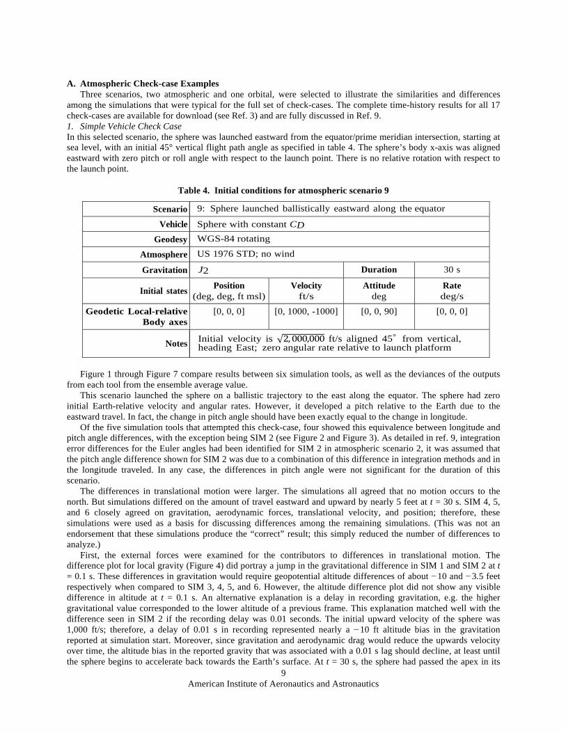
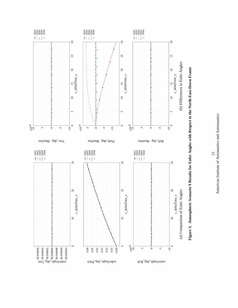
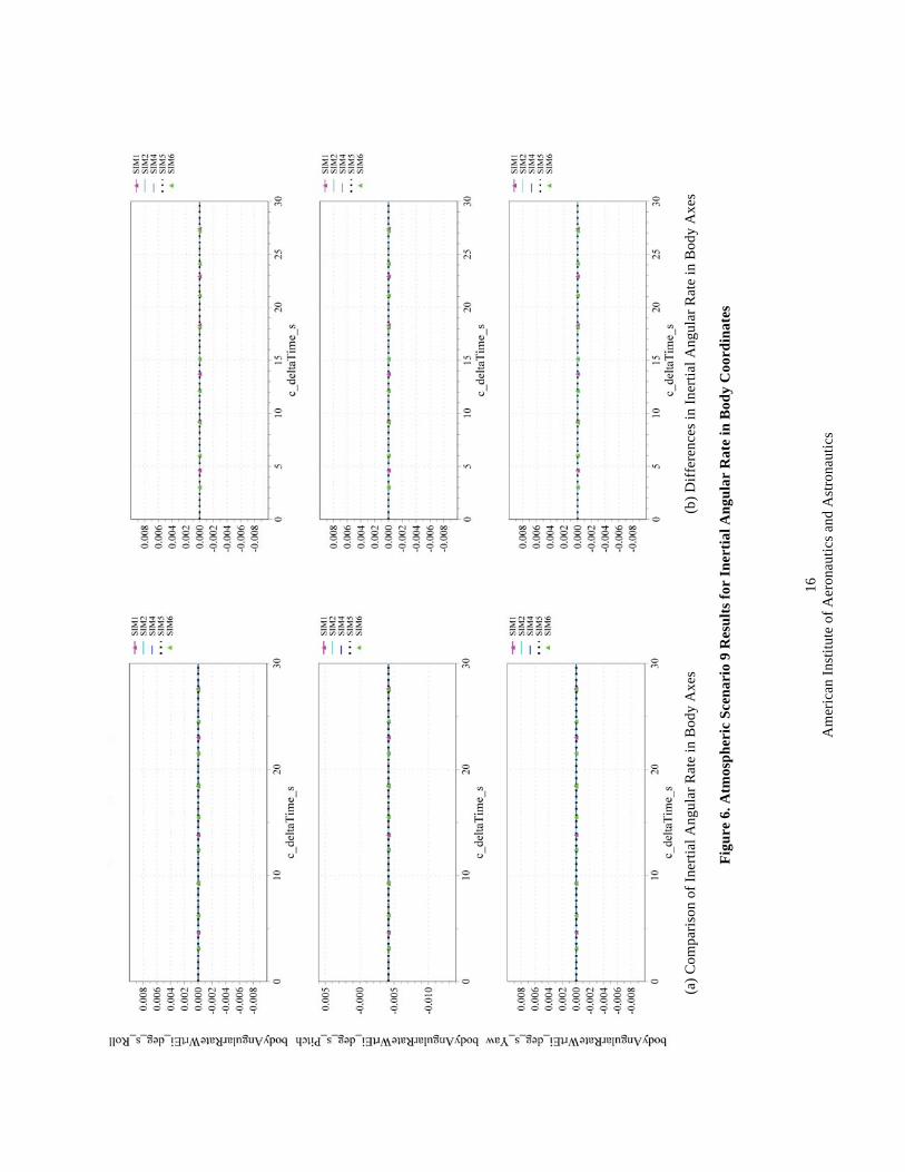
Figure 1 through Figure 7 compare results between six simulation tools, as well as the deviances of the outputs
from each tool from the ensemble average value. This scenario launched the sphere on a ballistic trajectory to the east along the equator. The sphere had zero
initial Earth-relative velocity and angular rates. However, it developed a pitch relative to the Earth due to the eastward travel. In fact, the change in pitch angle should have been exactly equal to the change in longitude.
Of the five simulation tools that attempted this check-case, four showed this equivalence between longitude and pitch angle differences, with the exception being SIM 2 (see Figure 2 and Figure 3). As detailed in ref. 9, integration error differences for the Euler angles had been identified for SIM 2 in atmospheric scenario 2, it was assumed that the pitch angle difference shown for SIM 2 was due to a combination of this difference in integration methods and in the longitude traveled. In any case, the differences in pitch angle were not significant for the duration of this scenario.
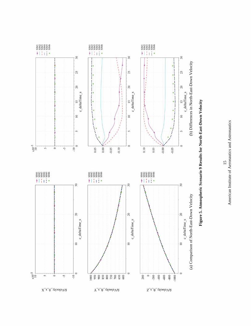
The differences in translational motion were larger. The simulations all agreed that no motion occurs to the north. But simulations differed on the amount of travel eastward and upward by nearly 5 feet at t = 30 s. SIM 4, 5, and 6 closely agreed on gravitation, aerodynamic forces, translational velocity, and position; therefore, these simulations were used as a basis for discussing differences among the remaining simulations. (This was not an endorsement that these simulations produce the “correct” result; this simply reduced the number of differences to analyze.)
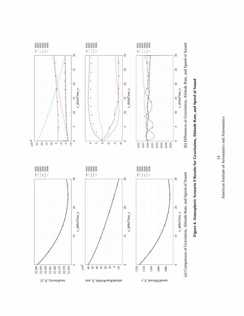
First, the external forces were examined for the contributors to differences in translational motion. The difference plot for local gravity (Figure 4) did portray a jump in the gravitational difference in SIM 1 and SIM 2 at t = 0.1 s. These differences in gravitation would require geopotential altitude differences of about −10 and −3.5 feet respectively when compared to SIM 3, 4, 5, and 6. However, the altitude difference plot did not show any visible difference in altitude at t = 0.1 s. An alternative explanation is a delay in recording gravitation, e.g. the higher gravitational value corresponded to the lower altitude of a previous frame. This explanation matched well with the difference seen in SIM 2 if the recording delay was 0.01 seconds. The initial upward velocity of the sphere was 1,000 ft/s; therefore, a delay of 0.01 s in recording represented nearly a −10 ft altitude bias in the gravitation reported at simulation start. Moreover, since gravitation and aerodynamic drag would reduce the upwards velocity over time, the altitude bias in the reported gravity that was associated with a 0.01 s lag should decline, at least until the sphere begins to accelerate back towards the Earth’s surface. At t = 30 s, the sphere had passed the apex in its
American Institute of Aeronautics and Astronautics
10
trajectory but the downward velocity remained low. The altitude bias for a 0.01 s delay would be +1.8 ft. However, at the same time, SIM 2 showed an altitude difference that had grown to approximately 1.4 feet, relative to the consensus group (SIM 4/5/6) (Figure 2). The altitude difference, therefore, largely canceled the altitude bias from the recording lag and the difference in gravitation between SIM 2 and SIM 4/5/6 at t = 30 seconds was reduced to nearly zero, as shown on the plots (Figure 4). The “recording delay” also appeared to explain the gravitation differences in SIM 1 but the required delay would have needed to be about 0.004 s which is not a frame rate reported by the simulation. Furthermore, SIM 1 did not exhibit a steady decline in gravitation difference; instead, the gravitation difference exhibited a slight increase over time (Figure 4). This likely occurred because the altitude difference between SIM 1 and SIM 4/5/6 was increasing in a direction that initially compensates for and then exceeded the decline in the lag-induced altitude bias.
Remaining differences in gravitation among the simulations were consistent with the plotted differences in altitude. In any case, even if the largest gravitation differences (which appeared to be due to recording delay) were applied to the EOM, they would account for differences in downward-axis velocity and altitude of less than 0.0005 ft/s and 0.009 ft, respectively, at t = 30 seconds. Thus, gravitation differences were not a driving contributor to differences in translational motion.
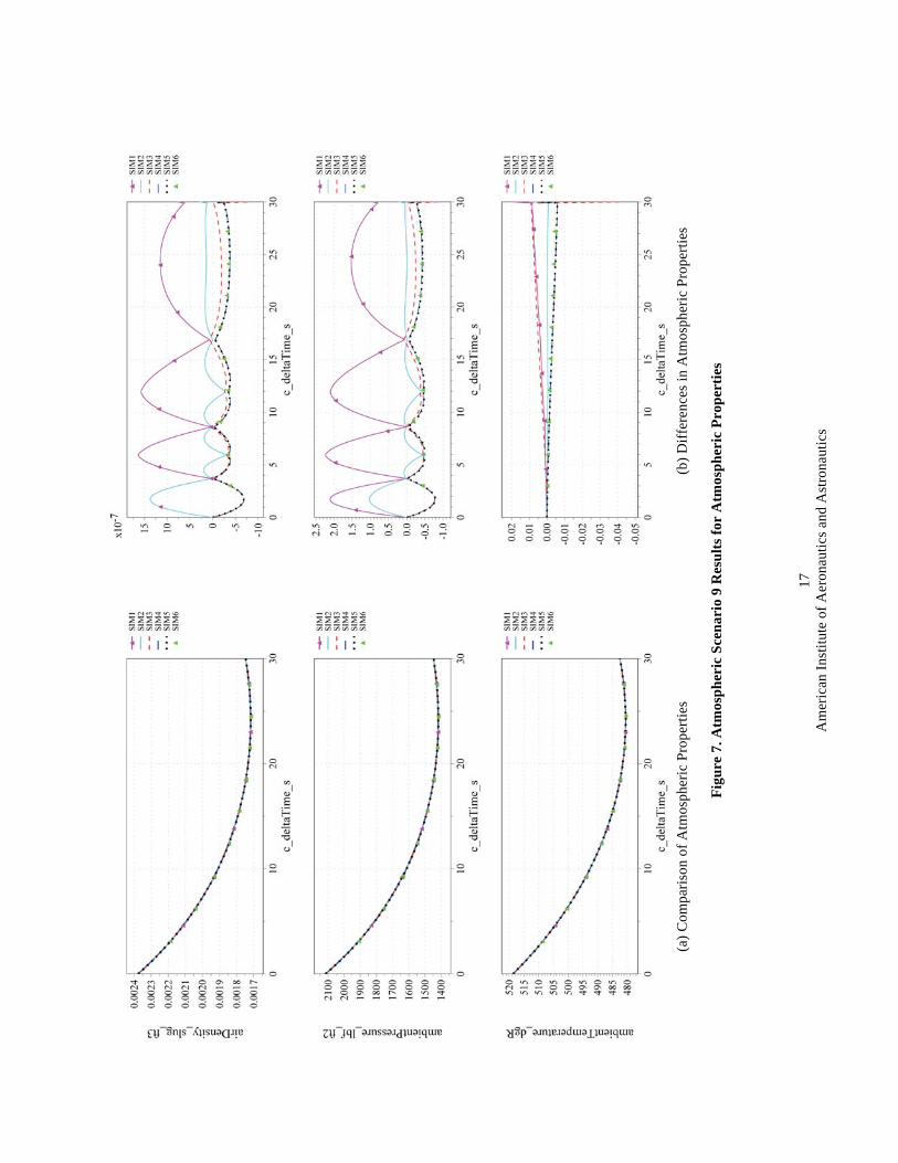
Differences in aerodynamic forces were larger than those for gravitation. The differences in SIM 2 aerodynamic forces had two main contributors, a 0.01 s delay in the recorded forces and a difference in atmospheric density. The delay was a recording artifact only and did not contribute to differences in velocity and position. The difference in atmospheric density derived from implementing the atmosphere model using a lookup table (Figure 7). From the data, it appears that SIM 2 used 1,000 m for the first break-point but every break-point thereafter was at 500 m increments. Small aerodynamic force differences (Figure 1) arising from differences in atmospheric density were the primary contributor for differences in translational motion between SIM 2 and SIM 4/5/6; they accounted for nearly all of the differences in velocity (Figure 5) and position (Figure 2) relative to SIM 4/5/6.
SIM 1 also used a lookup table to estimate atmospheric density; the lookup table has 1000 m breakpoints throughout the altitudes traversed in this case (Figure 7). The density difference was the primary contributor to the difference in aerodynamic forces between SIM 1 and SIM 4/5/6 (Figure 1). The evolving difference in velocity was a secondary contributor (Figure 5). However, the aerodynamic force differences for SIM 1 would only account for only 61% of the eastward velocity and longitude differences, 34% of the downward velocity difference, and 46% of the altitude difference.
The source of the remaining difference between SIM 1 and the SIM 4/5/6 group in translational motion could not be identified from the recorded data. The remaining contributor is likely an unknown difference in EOM implementation or configuration possibly including, but not limited to, differences in integration or other numerical methods.
Differences in aerodynamic forces (Figure 1) in SIM 3 were largely a response to the growing differences in velocity and altitude (which determined atmospheric density). A small difference in orientation of SIM 3 relative to SIM 4/5/6 also contributed to the differences in aerodynamic forces. Although SIM 3 values for Euler angles are not plotted, the SIM 3 data file had a very small initial roll angle (−6.4×10⁻⁶ degrees). This small roll angle likely explained the difference of order 1 × 10⁻⁷ lbf seen in body y-axis aerodynamic force (Figure 1). Nevertheless, the orientation difference did not contribute to differences in translational velocity and position. Relative to SIM 4/5/6, the expected contributions of the aerodynamic force differences to differences in translational motion at t = 30 seconds were +0.14 ft/s in eastward velocity, +6.4×10⁻⁶ degrees in longitude, −0.098 ft/s in downward velocity, and +1.8 ft in altitude. However, the total differences were larger and in the opposite direction. They were −0.16 ft/s in eastward velocity, −1.4 × 10⁻⁵ degrees in longitude, +0.14 ft/s in downward velocity, and −4.3 ft in altitude. As with SIM 2, the additional contributor(s) to these small differences could not be identified using the recorded data; it is also likely an unknown difference in EOM implementation or configuration including, but not limited to, differences in integration or other numerical methods.

A
mer
ican
Inst
itute
of A
eron
autic
s and
Ast
rona
utic
s 11
(a) C
ompa
rison
of A
erod
ynam
ic F
orce
s (b
) Diff
eren
ces i
n A
erod
ynam
ic F
orce
s
Figu
re 1
. Atm
osph
eric
Sce
nari
o 9
Res
ults
for
Aer
odyn
amic
For
ces
A
mer
ican
Inst
itute
of A
eron
autic
s and
Ast
rona
utic
s 12
(a) C
ompa
rison
of G
eode
tic P
ositi
on
(b) D
iffer
ence
s in
Geo
detic
Pos
ition
Figu
re 2
. A
tmos
pher
ic S
cena
rio
9 R
esul
ts fo
r G
eode
tic P
ositi
on
A
mer
ican
Inst
itute
of A
eron
autic
s and
Ast
rona
utic
s 13
(a) C
ompa
rison
of E
uler
Ang
les
(b) D
iffer
ence
s in
Eule
r Ang
les
Figu
re 3
. A
tmos
pher
ic S
cena
rio
9 R
esul
ts fo
r E
uler
Ang
les w
ith R
espe
ct to
the
Nor
th-E
ast-
Dow
n Fr
ame
A
mer
ican
Inst
itute
of A
eron
autic
s and
Ast
rona
utic
s 14
(a) C
ompa
rison
of G
ravi
atio
n, A
ltitu
de R
ate,
and
Spe
ed o
f Sou
nd
(b) D
iffer
ence
s in
Gra
vita
tion,
Alti
tude
Rat
e, a
nd S
peed
of S
ound
Figu
re 4
. Atm
osph
eric
Sce
nari
o 9
Res
ults
for
Gra
vita
tion,
Alti
tude
Rat
e, a
nd S
peed
of S
ound
A
mer
ican
Inst
itute
of A
eron
autic
s and
Ast
rona
utic
s 15
(a) C
ompa
rison
of N
orth
-Eas
t-Dow
n V
eloc
ity
(b) D
iffer
ence
s in
Nor
th-E
ast-D
own
Vel
ocity
Figu
re 5
. Atm
osph
eric
Sce
nari
o 9
Res
ults
for
Nor
th-E
ast-
Dow
n V
eloc
ity
A
mer
ican
Inst
itute
of A
eron
autic
s and
Ast
rona
utic
s 16
(a) C
ompa
rison
of I
nerti
al A
ngul
ar R
ate
in B
ody
Axe
s (b
) Diff
eren
ces i
n In
ertia
l Ang
ular
Rat
e in
Bod
y A
xes
Figu
re 6
. Atm
osph
eric
Sce
nari
o 9
Res
ults
for
Iner
tial A
ngul
ar R
ate
in B
ody
Coo
rdin
ates
A
mer
ican
Inst
itute
of A
eron
autic
s and
Ast
rona
utic
s 17
(a) C
ompa
rison
of A
tmos
pher
ic P
rope
rties
(b
) Diff
eren
ces i
n A
tmos
pher
ic P
rope
rties
Figu
re 7
. Atm
osph
eric
Sce
nari
o 9
Res
ults
for
Atm
osph
eric
Pro
pert
ies
American Institute of Aeronautics and Astronautics
18
2. F-16 Check Case
This selected scenario utilized the F-16 model. The vehicle was to be uncontrolled, as this was a test of how well the vehicle was trimmed for straight and level flight for non-trivial initial conditions (given in Table 5): positioned 10,000 ft above First Flight airport in Kitty Hawk, NC on a heading of 45° true at 400 kt true airspeed (KTAS) relative to the still atmosphere.
Each simulation’s trim solver solved for zero linear and angular accelerations (1 g flight) at 400 KTAS at 10,013 ft MSL by varying pitch attitude, elevator position, and throttle setting.
Table 5. Initial conditions for atmospheric scenario 11.
Scenario 11: Subsonic winged flight (trimmed straight & level)
Vehicle Unaugmented F-16
Geodesy WGS-84 rotating
Atmosphere US 1976 STD; no wind
Gravitation J2 Duration 180 s
Initial states Position (deg, deg, ft msl)
Velocity ft/s
Attitude deg
Rate deg/s
Geodetic Local-relative Body axes
[36.01916667, -75.67444444, 10013] [400, 400, 0] [0, 0, 45] [0, 0, 0]
Notes Initial position is 10,000 ft above KFFA airport (13’ MSL) on a 45◦ true course. True airspeed 335.15 knots. Stability augmentation off. Test of trim solution.
This check-case was the first of a series utilizing the F-16 model. Unlike the first ten atmospheric scenarios, the
F-16 scenarios required that the simulation tool generate an equilibrium (“trim”) solution for the F- 16 vehicle model so that its initial state, including control surface deflections and engine thrust, resulted in straight and level flight. This equilibrium solution requirement can introduce differences among the simulation implementations since different simulation tools may have different definitions for straight and level flight, especially over the curved surface of a round or ellipsoidal Earth. Simulation tools may also generate solutions with different tolerances for residual acceleration.
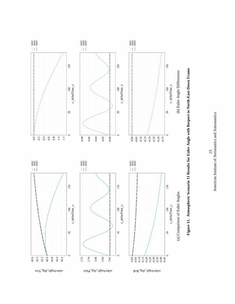
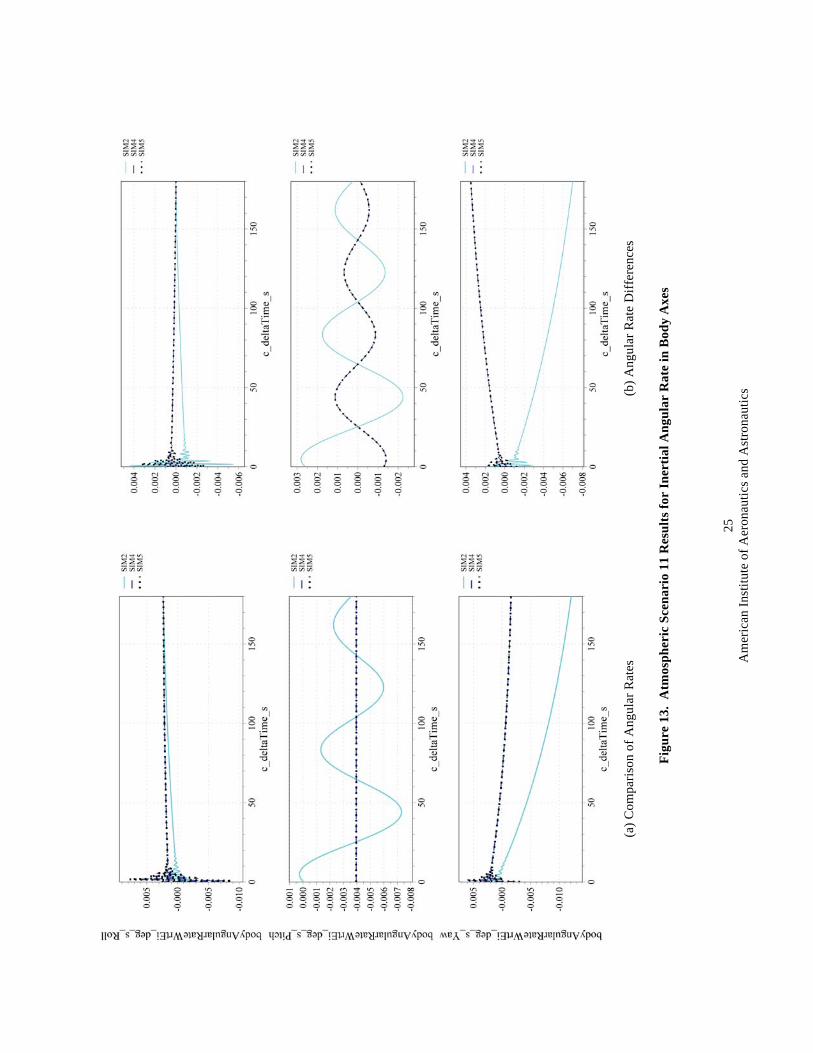
Such differences can be seen in Figure 8 through Figure 13 for the three simulations that provided data for this check-case. All three simulations used slightly different assumptions about the angular rate necessary for straight and level flight (Figure 13). SIM 2 constrained the angular rate to be zero in the inertial frame. SIM 4 solved for the pitch rate that maintained the pitch angle as the vehicle flew over the curved surface of the Earth. SIM 5 solved for the three-axis angular rate that maintained the vehicle orientation (i.e. all three Euler angles) relative to the local vertical frame as the vehicle flew over the curved surface of the Earth. Even so, the equilibrium roll and yaw rate computed by SIM 5 were very small, 3 × 10⁻⁵ and 8 × 10⁻⁴ deg/s respectively. Therefore, the equilibrium solutions for SIM 4 and SIM 5 were nearly identical. Nevertheless, each simulation exhibited an oscillation in angular rates during the first second of the simulation. Differences during the oscillation dwarfed the initial attitude differences. Once the oscillation settled, however, SIM 4 and SIM 5 were in near agreement on angular rate while the trajectory calculated by SIM 2 continued to differ from SIM 4/5.
The initial roll and pitch angle in SIM 2 also differed from SIM 4/5 (Figure 11). The root cause was a difference in the simulated gravity vector. SIM 2 employed a simplification that creates a gravity vector that is slightly deflected from the surface normal. (Here, the terms gravitation and gravity have different meanings: gravitation is the force from the attraction of two masses; gravity is the sum of gravitation and the centrifugal acceleration due to the Earth’s rotation. Gravity is the acceleration of a body in free fall measured by an observer stationed on the surface of the Earth.) All three simulations computed the geocentric gradient of the J2 gravitation potential, which produced gravitation in the geocentric down direction and a much smaller contribution in the geocentric north direction. However, SIM 2 approximated the geodetic NED frame using the geocentric frame as the local vertical local horizontal (LVLH) frame when computing gravity. SIM 4 and SIM 5 translated the geocentric gravitation vector into a geodetic gravitation vector. This rotation was necessary to produce a gravitation vector where the

American Institute of Aeronautics and Astronautics
19
resulting small geodetic north-axis component of gravitation was canceled by the geodetic north-axis contribution of centrifugal acceleration due to the Earth’s rotation. This resulted in a gravity vector whose direction matched the geodetic down-axis direction almost exactly. Without rotation to the geodetic frame, the gravitation and centrifugal acceleration combined to create a gravity vector slightly deflected from the geocentric downward direction. That deflection was equal to the difference between the geodetic and geocentric latitude since the true direction of the gravity vector is along the geodetic normal.
In the initial position specified by this check-case, the resulting gravity vector, in geocentric coordinates, is deflected 0.18 degrees southward of the radial vector. That deflection amount was approximately equal to the difference in roll angle between SIM 2 and SIM 4/5. The equilibrium solver for SIM 2 appeared to roll the vehicle slightly so that its aerodynamic lift was more closely aligned with the slightly non-vertical gravity vector. The SIM 2 equilibrium solver also produced a slightly different pitch angle because the aerodynamic lift required for the trim solution differed slightly from those of SIM 4/5. With a non-zero roll angle, eliminating vertical acceleration in SIM 2 required balancing contributions from weight, thrust, lift, drag, and aerodynamic side force. When the roll angle was zero, as in SIM 4 and 5, no significant aerodynamic side force was generated.
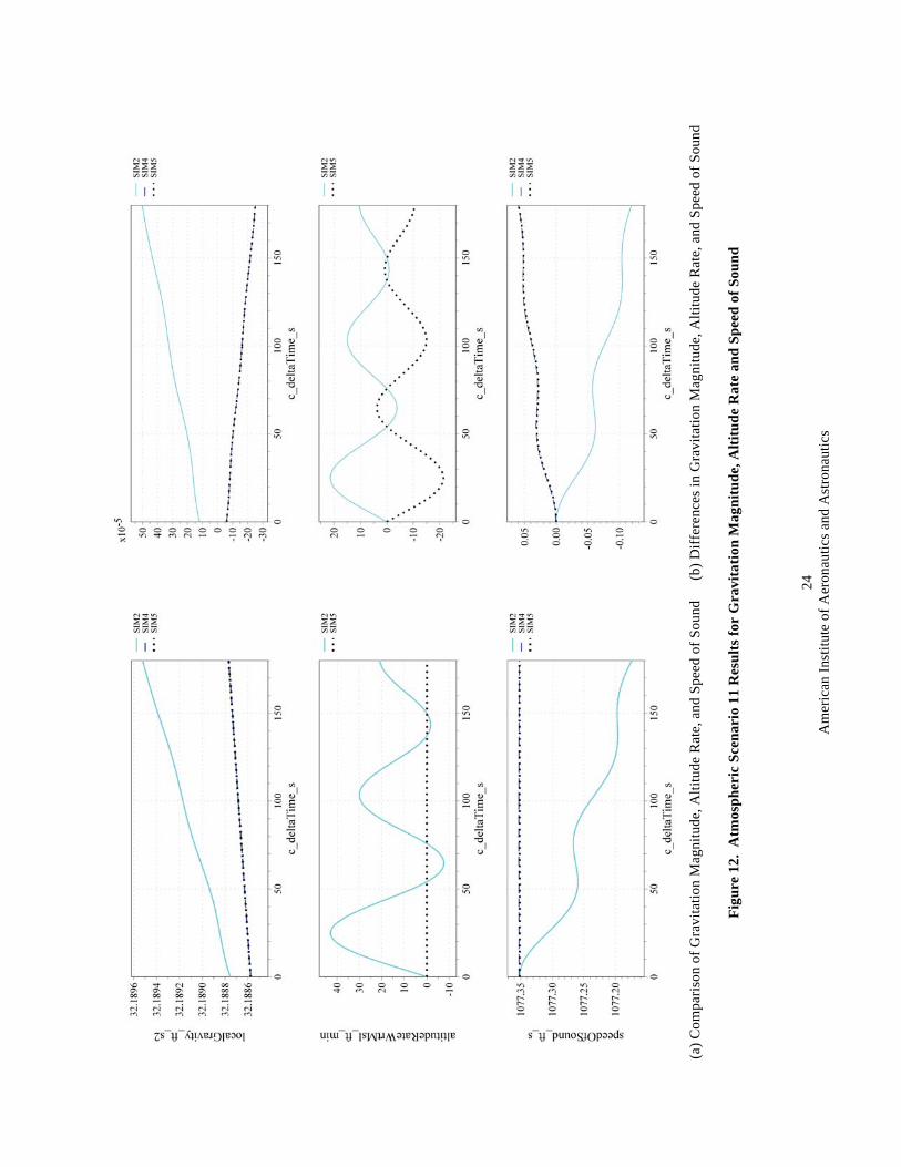
Even if SIM 2 were modified to use a geodetic gravity vector, the difference plot for gravitation (Figure 12) shows that there would remain a small difference in gravitation of 1.8 × 10⁻⁴ ft/s2. There should be no difference in Earth parameters among the simulations given that the simulations match J2 gravitation for atmospheric case 1 as described in Ref. 9. What remains as a possible explanation of this difference in gravitation could be a difference in the conversion from the initial geodetic coordinates to an initial geocentric position. The difference could be significant. For example, a reduction of 58 feet in the geocentric distance of the vehicle would produce the same change in magnitude. Nevertheless, the difference in magnitude should be a minor contributor to the vehicle dynamics as it adds only 0.11 lbf to the weight of the 20,500 lb F-16 example vehicle.
Differences in initial angular rates would induce differences in the aerodynamic forces and moments. However, those differences were very small and were dwarfed by other contributors including the contribution from the angular rate oscillation in the first second of the simulation (Figure 13).
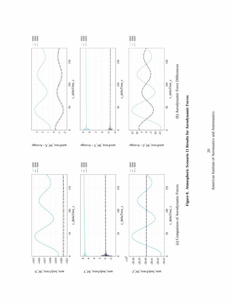
A substantial difference in the plotted aerodynamic moments (Figure 9) is the result of a difference in the reference location for recording aerodynamic moments. When recording the aerodynamic moments, SIM 2 recorded moments about the aerodynamic moment reference center (MRC); SIM 4 and 5 recorded the aerodynamic moment at the vehicle center of mass (CM) after these had been transferred from the MRC. This difference appears in the aerodynamic moment plots for all the F-16 cases; it just reflects a lack of agreement on which moment vector to record.
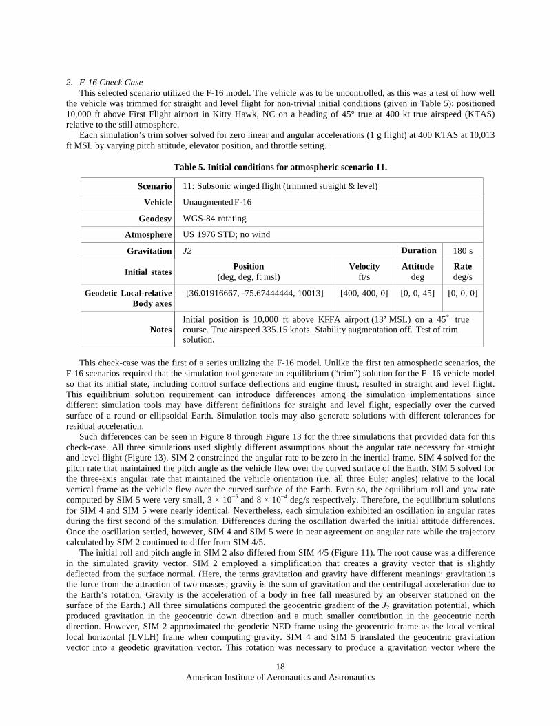
Even when the moments were adjusted for differences in the reference point, a difference in the initial aerodynamic yaw and pitching moments remained between SIM 2 and SIM 4/5 at the MRC; furthermore, SIM 2 also differed in the initial aerodynamic forces (Figure 8). These differences resulted from the difference in the gravity vector as described previously. With the gravity vector deflected from the local vertical in SIM 2, SIM 2 required a trade-off in pitch angle and roll angle to create the right combination of angle of attack and sideslip such that the resulting aerodynamic lift and side-force counteracted the gravity vector while leaving no residual force in the horizontal plane. As discussed above, the result is a roll angle that nearly aligned the body z-axis with the deflected gravity vector. The differing lift required a different aerodynamic pitching moment to counteract the lift-induced pitching moment at the CM. The resulting aerodynamic side force also induced a yawing moment at the CM and therefore required a counteracting aerodynamic yawing moment which was not present in SIM 4 and SIM 5. That yawing moment was achieved, in SIM 2, by setting the rudder to a non-zero initial value.
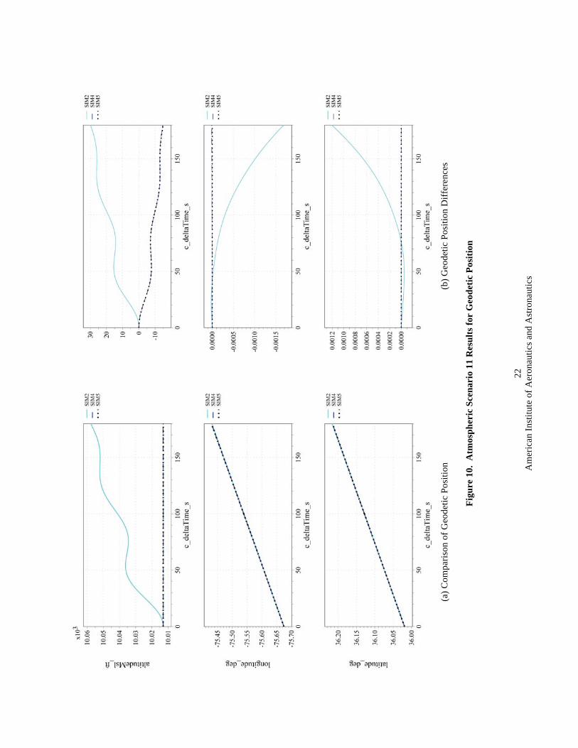
The above differences, in general, set SIM 2 on a different trajectory from SIM 4 and SIM 5. After 180 seconds, the difference in vehicle positions between SIM 2 and SIM 4/5 was approximately 666 feet according to the recorded values of latitude, longitude, and altitude (Figure 10). The position difference between SIM 4 and 5 at the end of the scenario was two orders of magnitude smaller, at approximately 4 ft.
A
mer
ican
Inst
itute
of A
eron
autic
s and
Ast
rona
utic
s 20
(a) C
ompa
rison
of A
erod
ynam
ic F
orce
s (b
) Aer
odyn
amic
For
ce D
iffer
ence
s
Figu
re 8
. A
tmos
pher
ic S
cena
rio
11 R
esul
ts fo
r A
erod
ynam
ic F
orce
s
A
mer
ican
Inst
itute
of A
eron
autic
s and
Ast
rona
utic
s 21
(a) C
ompa
rison
of A
erod
ynam
ic M
omen
ts
(b) A
erod
ynam
ic M
omen
t Diff
eren
ces
Figu
re 9
. A
tmos
pher
ic S
cena
rio
11 R
esul
ts fo
r A
erod
ynam
ics M
omen
ts
A
mer
ican
Inst
itute
of A
eron
autic
s and
Ast
rona
utic
s 22
(a) C
ompa
rison
of G
eode
tic P
ositi
on
(b) G
eode
tic P
ositi
on D
iffer
ence
s
Figu
re 1
0. A
tmos
pher
ic S
cena
rio
11 R
esul
ts fo
r G
eode
tic P
ositi
on
A
mer
ican
Inst
itute
of A
eron
autic
s and
Ast
rona
utic
s 23
(a) C
ompa
rison
of E
uler
Ang
les
(b) E
uler
Ang
le D
iffer
ence
s
Figu
re 1
1. A
tmos
pher
ic S
cena
rio
11 R
esul
ts fo
r E
uler
Ang
le w
ith R
espe
ct to
Nor
th-E
ast-
Dow
n Fr
ame
A
mer
ican
Inst
itute
of A
eron
autic
s and
Ast
rona
utic
s 24
(a) C
ompa
rison
of G
ravi
tatio
n M
agni
tude
, Alti
tude
Rat
e, a
nd S
peed
of S
ound
(b
) Diff
eren
ces i
n G
ravi
tatio
n M
agni
tude
, Alti
tude
Rat
e, a
nd S
peed
of S
ound
Figu
re 1
2. A
tmos
pher
ic S
cena
rio
11 R
esul
ts fo
r G
ravi
tatio
n M
agni
tude
, Alti
tude
Rat
e an
d Sp
eed
of S
ound
A
mer
ican
Inst
itute
of A
eron
autic
s and
Ast
rona
utic
s 25
(a) C
ompa
rison
of A
ngul
ar R
ates
(b
) Ang
ular
Rat
e D
iffer
ence
s
Figu
re 1
3. A
tmos
pher
ic S
cena
rio
11 R
esul
ts fo
r In
ertia
l Ang
ular
Rat
e in
Bod
y A
xes

American Institute of Aeronautics and Astronautics
26
B. Orbital Check-case Examples There is less variation in the results among the simulations participating in the orbital cases. Therefore, a single
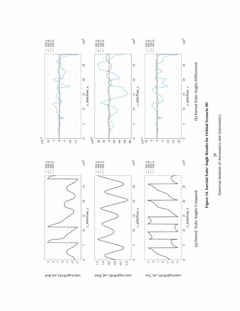
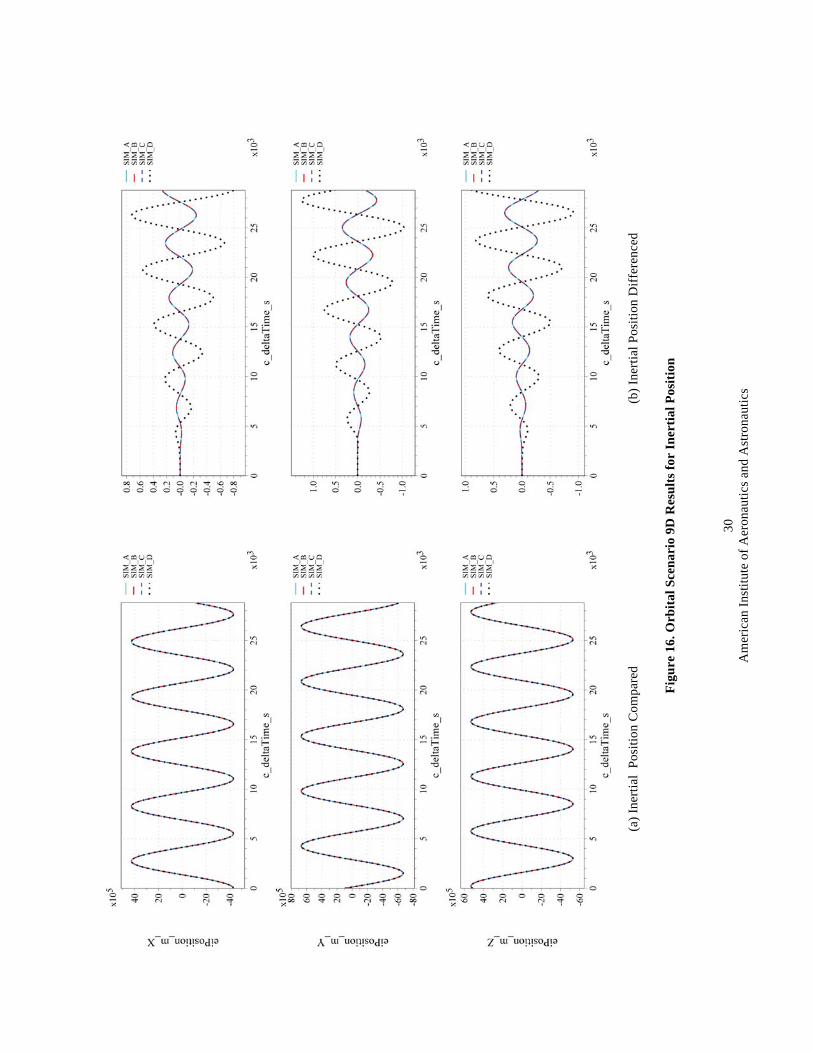
case is presented to typify the outcome of the simulation comparison (all 27 check-cases are discussed in detail in reference 9 and data sets are available at the URL specified by reference 3). The selected orbital check-case is 9D which exercised both translational and rotational motion by applying both a square pulse thrust and a square pulse torque to the representative ISS mass. The detailed conditions of this check case are provided in Table 6; details on the parameters for the Earth and terrestrial time are found in Table 73 of Ref. 9. In this check case, the vehicle begins in a nearly circular orbit with an initial inertial rotation that attempts to maintain the vehicle orientation relative to the orbit. At t = 1000 s, this check-case applied a force of 10 N in the positive body x-axis direction through the vehicle's center of mass and a torque of 10 N-m about the positive body x-axis. The external force and torque were applied for an additional 1000 s, then were set to zero for the remainder of the run.
Table 6. Orbital Scenario 9D Description
vehicle type ISS orbit type nearly circular atmosphere model Off aerodynamic drag Off gravitational model inverse-square gravity gradient Off sun/moon gravitational perturbations Off Initial inertial rotation rate (body axis) [0.000000; -0.065000; 0.000000] deg/s Initial LVLH attitude (3-2-1 Euler sequence) [0.000000; -11.600000; 0.000000] deg Initial inertial position [-4,292,653.4; 955,168.47; 5,139,356.57] m Initial inertial velocity [109.649663; -7,527.726490; 1,484.521489] m/s Start Time (UTC) 2007/324:00:00:00
Select results are provided in Figure 14 through Figure 16. One challenge that this check case presented to a
simulation is the modeling of the force and torque as a square pulse. The integration error of a numerical integration technique can increase substantially as it encounters the discontinuous leading and trailing edges of the square pulse. Furthermore, a one-frame lead or lag in the start or end of the square pulse causes a substantial difference in the results that follow. Some early iterations in the comparison were spent establishing and confirming the exact timing of the leading and trailing edge of the square pulses among the simulations.
Figure 14 shows the predicted orbit-relative attitude of the vehicle presented as LVLH Euler Angles. SIM B and SIM C agreed on the vehicle attitude; differences between them were negligible. Compared to SIM B and C, SIM D exhibited a minute difference in angular momentum at the leading edge of the torque pulse (as evidenced by the inertial angular rates in Figure 15) but remained steady after the trailing edge of the input. The amplitude and duration of the difference in angular momentum caused the momentary spike in difference for LVLH Euler angles, but the long-term increase in difference was very modest. Moreover, these differences were considered insignificant. SIM A shows a minute difference in angular momentum, relative to the other simulations, after completing the torque pulse (see the angular rate differences in Figure 15). The difference in angular moment is likely caused by a difference in integration method. This minute difference in angular momentum caused the increasing difference in the LVLH Euler angles over time. As detailed in Ref. 9, results for prior orbital check-case 8B reveal that, under torque-free rotation, differences in integration methods among the simulations contribute to differences in Euler Angles of order up to 10-5 radians, and those differences would also manifest here. Nevertheless, the overall differences in attitude for this case were not significant.
Differences in rotational rates between the simulations were negligible and were attributed to differences in integration method as explained in the previous paragraph or differences in the precision of the recorded data. The one exception was the difference in the initial inertial pitch rate for SIM D (see Figure 15). Although hard to see in the plots, SIM D recorded a sudden jump in pitch rate from 0 rad/s at t = 0 to 0.0011 rad/s at t = 60 s (the next recorded frame). However, this jump appeared to be an artifact of the data recording as the Euler angles showed no response to this jump. Nevertheless, this jump was sufficiently large to require the comparison plots to use a range that was too large to display the differences between the simulations in the rest of the maneuver. Even so, those differences were similar in magnitude to the differences seen in the roll and yaw rates.

American Institute of Aeronautics and Astronautics
27
For SIM B, SIM C, and SIM D, those rotational state differences did not contribute significantly to the differences in translational state, as a result of influencing the direction of the thrust vector. The differences in translational state among these simulations were negligible as evidenced by the inertial position differences in Figure 16. SIM A, however, exhibited Euler angle differences due to integration residuals that caused the inertial position to depart slightly from the other solutions. The inertial position difference grew to less than 2 meters at the end of the simulated eight hour flight. However, the differences are entirely attributed to the combined integration residuals for both the rotational and translational motion, and not to any differences in modeling or equations of motion. Thus, whether it was SIM A or the other three simulations exhibiting increased integration residue, the integrators could likely be reconfigured to reduce the difference in position if an application required greater accuracy in results.
A
mer
ican
Inst
itute
of A
eron
autic
s and
Ast
rona
utic
s 28
(a) I
nerti
al E
uler
Ang
les C
ompa
red
(b) I
nerti
al E
uler
Ang
les D
iffer
ence
d
Figu
re 1
4. In
ertia
l Eul
er A
ngle
Res
ults
for
Orb
ital S
cena
rio
9D

A
mer
ican
Inst
itute
of A
eron
autic
s and
Ast
rona
utic
s 29
(a) I
nerti
al A
ngul
ar R
ates
Com
pare
d (b
) Ine
rtial
Ang
ular
Rat
es D
iffer
ence
d
Figu
re 1
5 O
rbita
l Sce
nari
o 9D
Res
ults
for
Iner
tial A
ngul
ar R
ate
in B
ody
Coo
rdin
ates
A
mer
ican
Inst
itute
of A
eron
autic
s and
Ast
rona
utic
s 30
(a) I
nerti
al P
ositi
on C
ompa
red
(b) I
nerti
al P
ositi
on D
iffer
ence
d
Figu
re 1
6. O
rbita
l Sce
nari
o 9D
Res
ults
for
Iner
tial P
ositi
on
American Institute of Aeronautics and Astronautics
31
IV. Summarized Results A ground rule used by the team in providing comparisons was that at least three simulation tools had to submit
results for each check-case before it could be analyzed. Additional planned cases (e.g., supersonic fighter maneuvering flight and a proposed Apollo-like capsule reentry) were not included due to an insufficient number of implementations achieved. A total of 16 of the 17 atmospheric check cases were completed and all of the 27 orbit check cases were completed.
A. Atmospheric check-case results In general, comparisons of the atmospheric check-cases as simulated by several simulation tools indicate minor
differences due to two variations in implementation: tabular versus equation-based atmosphere models, and geodetic versus geocentric geometries.
In earlier computationally-constrained simulation implementations, an atmosphere model (e.g., Ref. 7 employed for these atmospheric flight simulations) was implemented as a table of density, temperature, and pressure values as a function of geometric height above a reference surface. This table was used in a linear interpolation between altitudes since this was typically faster than performing the complex calculations necessary to determine these quantities algebraically. Improved processors have made the direct calculation approach economically feasible and more precise. However, several of the participating simulation tools continue to use an atmospheric table implementation. Therefore, some of the trajectory differences are due to linear interpolation of atmospheric properties.
The other main difference between results in atmospheric comparisons is an artifact of historical simulation techniques. As mentioned, early digital flight simulations of subsonic aircraft often assumed a flat Earth, where latitude and longitude were directly related to a Cartesian grid in the vicinity of a runway or airport. This was an appropriate approximation for low-speed flight in the vicinity of and while maneuvering around the terminal environment. Since the check-cases specified at least a round Earth, some retrofitting was undertaken to adapt the flat-Earth approximations in some participants to a round or oblate Earth. However, some artifacts of the simpler geodesy assumption remain which affect geodetic coordinate calculations and the direction of gravity relative to the local vertical.
To a smaller degree, some variances in the implementation of the square-law and harmonic gravitation were due to differences in gravitation model implementation, or in the conversion of the initial geodetic position into the geocentric position. Another variance source in the F-16 check-cases was differences in defining the equilibrium (i.e., trim) values for straight and level flight, especially the trimmed rotational rate.
Errors in participating simulation tools that were initially uncovered, and corrected, included mistakes in gravitational models, incorrect or imprecise initial condition values and geophysical constants, a one-frame time shift in gravitational value, and a transposition error in atmospheric property tables. For example, one simulation routinely and incorrectly aligned gravitational attraction along the geocentric radius axis, not the geodetic nadir. This led to a very, very small difference in the resulting trajectories that might not have been quickly identified without this exercise.
Finally, differences in numerical integration methods in the simulation tools appeared to cause trajectory differences. These differences are hypothesized, as no specification of (or sufficient data regarding) integration techniques was initially available.
In all cases, these differences were minor. Most were only visible when plotting variances between individual simulation results versus consensus or averaged results.
It should be noted that obtaining correlation between these simulations was an iterative process. Initial results were not as good as those ultimately obtained due to ambiguity in specification or implementation of initial conditions, maneuver inputs, and other simulation implementation differences.
A total of 84 trajectories were generated, comprised of nearly four million data points; these data sets are stored in 64 MB of data files available in the data repository3.
B. Orbital Check-Case Results Comparison of orbital check-cases showed good comparisons with few significant differences. As with the
atmospheric cases, some iteration was required as significantly different results were initially obtained. These differences included use of different revisions of the MET model, differences in the specification of the Earth’s
American Institute of Aeronautics and Astronautics
32
position at the start of various scenarios, differences in integration technique, or to misinterpreting a sign convention or initial condition specification.
An error was discovered (and corrected) in one of participating simulation tools in which an external force or moment was applied for a length of time other than what was specified in the configuration. This error was introduced in a recent rewrite of that particular module of the simulation tool and had somehow managed to elude detection, despite extensive regression tests that are routinely applied to all revisions. The revised tool had not yet been released, but the error may have affected NASA missions if it had not been detected during this exercise. The tool architect stated that he believed this ‘catch’, by itself, justified the cost of the exercise.
A total of 103 trajectories were generated and comprise nearly 1.4 million data points. These data sets are stored in 25 MB of data files available in the data repository3.
C. Comparison Difficulties During this exercise, it became apparent that the time required to reach a reasonable level of match had been
underestimated. The original schedule developed and agreed to by the team reflected the expectation to complete this effort in just over 12 months. The effort took 30 months and was not completed to the degree expected at the outset, in that one atmospheric check-case (Earth reentry from a lunar return trajectory) has not been attempted, and a second atmospheric case remains incomplete.
Part of the delay was due to the now-apparent need to specify initial conditions and maneuvering inputs exactly. It was believed early in the planning process that it would be sufficient for the scenarios to be described briefly in one axis frame; however, obtaining good matches ultimately required detailed specification of the initial conditions in several axis frames. An example is the initial rotation rate for some of the early atmospheric check-cases: a small numeric difference exists between the inertial and the ECEF angular rate of a body. Ensuring close matches required giving the rotation rate in both frames to ensure all simulation tools started with the same rate, since some simulation tools are initialized in ECEF-relative rates and others in inertial rates.
As knowledge was gained in this process, the initial conditions document had to be revised several times, initially leading to confusion by the team as to which version was to be used in each round of comparison plots, which delayed reaching successful matches.
The process followed by the geographically dispersed team also introduced delays. Due to the large amount of data involved, considerable time was spent uploading data sets from each tool to a central server, downloading and plotting the trajectories by one analyst, uploading the results, and downloading and inspecting the large number of resulting plots for differences. Obvious differences were fairly easy to detect, but determining the root cause of the difference often took considerable time and effort.
A formal comparison by one analyst required a period of several weeks, due to the large number of maneuvers to compare and the in-depth analysis required.
Since most participants were not assigned full-time on this exercise, some of these comparison cycles took longer than others due to NASA priorities. Many more comparison cycles were also required than originally expected (30 sets of comparison plots were generated for the atmospheric cases between May 2013 and August 2014).
V. Conclusion The eventual matches between simulation tools, achieved only after several iterations of comparing results and
correcting mistaken assumptions and other errors, were good enough to indicate agreement between a majority of simulation tools for all cases published. Most of the remaining differences are explained and could be reduced with further effort.
Simulations from atmospheric check cases found the following: • Minor differences in results from tabular versus equation-based atmosphere models, and geodetic versus
geocentric geometries; • To a smaller degree, some differences in the implementation of the square-law and harmonic gravitation are
also apparent due to differences in gravitation model implementation or in the conversion of the initial geodetic position into the geocentric position (since position is an input into the gravitation model);
• Due to differences in trim algorithms, some of the 6-DOF aircraft check-cases (cases 10-16) leave some remaining disagreements on precise numbers, but do indicate a family of solutions that are close enough to serve as a comparison with other simulation tools; and
• Differences in numerical integration methods in the different simulation tools appeared to cause some differences in predicted trajectories.
American Institute of Aeronautics and Astronautics
33
Comparison of simulations from the orbital check cases showed good agreement. The remaining differences are attributed to either an obvious misconfiguration of the simulation tool or differences in the numerical integration method and step size.
Lessons learned in this exercise include the following observations and recommendations for improving cross-simulation comparisons:
1. Modeling even simple vehicles posed challenges. Differences in the implementation of simple vehicle models were apparent. These arose primarily from differences in interpretation of the scenario and initial conditions. Initial attempts to model these scenarios led to some significant miscompares that revealed differences in physical constants and other modeling errors. These differences in constants and modeling errors were corrected in several tools with each comparison iteration.
2. It took significant effort to get good agreement on the check-cases. Even simple aerospace vehicle simulation models are non-trivial to implement. The comparable results shown in most of these check-cases required extensive iterations and adjustments/corrections to initial conditions and modeling assumptions.
3. Tabular versus equation-based atmosphere models introduced trajectory differences. 4. Different interpretations of nadir direction can lead to differences due to “non-vertical” gravitational
residue. 5. While the majority of atmospheric simulations appeared to use WGS-84 Earth geodesy, simplifications
in simulations originally designed for flat-Earth or round-Earth led to trajectory differences. Therefore, Flat-Earth or round-Earth simplifications should only be used when appropriate.
6. Precise specification of initial conditions would be assisted by a standard for specifying the state vector of a 6-DOF flight simulation. A convention or standard for numerical specification of unambiguous initial conditions for 6-DOF flight simulations should be developed to ensure multiple flight simulation tools start at exactly the same planet-relative position, velocity, attitude and angular rates. A significant portion of this exercise was spent resolving misinterpreted initial conditions despite an attempt to specify this information. Questions regarding whether an angular rate initial condition was with respect to a rotating Earth or to an inertial axis were raised multiple times, as well as ambiguity of initial angular attitude. Such as a standard for initial state vector description should employ ANSI/AIAA S-119-2011 for identifying simulation parameters, for ease of collaboration, and dynamic model data exchange.
7. In the atmospheric check cases, every simulation examined eventually matched trajectories with at least two other simulations to a reasonable degree, where the correlation level is a function of the simulation purpose.
8. In general, the orbital cases (implemented in at least three different simulation tools) matched fairly well, but minor differences are apparent.
9. In general, the atmospheric cases did not match as well as the orbital cases. Atmospheric flight is non-linear, due to forces and moments being related to the square of the air-relative vehicle velocity, and to other non-linear aerodynamic effects. The larger number of simulation tools applied to the atmospheric check cases increased the chances of mismatches.
10. The amount of effort required to develop, specify, and reconcile differences for multiple vehicle models across an array of simulation tools was grossly underestimated.
11. The comparison check-cases examined form the basis of a comprehensive set of verification data sets for 6-DOF flight simulations. Additional scenarios and results would improve the value of this process. One identified need is for supersonic maneuvering flight and atmospheric re-entry scenarios.
12. Nearly every simulation framework that participated in this exercise discovered at least one significant implementation difference/error that was modified/corrected to improve correlation with other simulation tools.
13. Some early problems with comparisons included different definitions among the simulation for similar sounding variable names in the recorded data. A structured, binary, compressed format to encode bulky time-history data (which is provided for this exercise as comma-separated-value Unicode text files at the URL identified by Ref. 3), as well as tools to manipulate this data, should be identified and/or developed and adopted to assist in sharing predicted trajectories from simulation tools. Using a CSV format was expeditious but cumbersome. Simulation comparisons would also benefit from employing ANSI/AIAA S-119-2011 for unambiguous identification of recorded parameters.
American Institute of Aeronautics and Astronautics
34
VI. References 1Anon.: Flight Dynamics Model Exchange Standard. ANSI/AIAA S-119-2011, American National Standard, Washington,
DC, March 2011. 2Jackson, E. Bruce Shelton, Dr. Robert, et al., “Development of Verifications Check-cases for Six-Degree-of-Freedom Flight
Vehicle Simulations,” AIAA paper 2013-5071, AIAA Modeling and Simulation Technologies Conference, August 2013. 3Anon.: Six degree-of-freedom (6-DOF) Flight Simulation Check Cases http://nescacademy.nasa.gov/flightsim/index.html,
NASA Engineering and Safety Center, 2014. 4Crues, Edwin Z.; Jackson, A. A.; and Morris, J. C.: “A Process for Comparing Dynamics of Distributed Space Systems
Simulations.” Joint 2009 Simulation Interoperability Workshop, San Diego, CA, 2009. 5Anon.: Department of Defense World Geodetic System 1984. NIMA TR8350.2, National Imagery and Mapping Agency,
Washington, DC, 2000. 6Seidelmann, P. Kenneth. Explanatory Supplement to the Astronomical Almanac: A Revision to the Explanatory Supplement
to the Astronomical Ephemeris and the American Ephemeris and Nautical Almanac. Sausalito, Calif: University Science, 2006. 7Anon.: US Standard Atmosphere 1976. NASA-TM-X-74335, Joint NOAA, NASA, and USAF publication, Washington,
DC, 1976. 8Jackson, E. B.: “Dynamic Aerospace Vehicle Exchange Markup Language.” AIAA Modeling and Simulation Technical
Committee, version 2.0.2 ed., July 2011. Available from http://daveml.org. 9Jackson, E. Bruce, Shelton, Dr. Robert A., et al., “Check-cases for Verification of Six-Degree-of-Freedom Flight Vehicle
Simulations,” NESC-RP-12-00770, 2014.
Recommended