Professor C. Magee, 2006Page 1
Lecture 11• Network terminology and structural characteristics
• Motifs (patterns of directed -and non-directed- links and a connection to function)
• A Complex system representation: hierarchy of function
• Coarse-Graining (abstractions of function hierarchicallydescribed) and PGNM
• Return to modularity discussion • (Introduction to models (lecture 12 material as time permits)
• Electric Power student team report #1
Professor C. Magee, 2006Page 2
Network Analysis Terminology -notated• node (vertex), link (edge) CM2, • size, sparseness, metrics CM2• degree, average degree, degree
sequence DW4• directed, simple DW4• geodesic, path length, graph
diameter DW4• transitivity (clustering), DW10
connectivity, reciprocity CM6• centrality (degree, closeness,
betweenness, information, eigenvector) CM6
• prestige, acquaintance CM6• ideal graphs (star, line, circle,
team) CM6• degree distribution, power laws,
exponents, truncation, CM6
• Models (random, “small world”, poisson, preferential attachment)
• constraints, rewiring DW7• Hierarchy DW7, JM8&9, CM11• community structure, cliques,
homophily, assortative mixing, degree correlation coefficient DW10
• motifs, coarse- graining CM11• navigation, search, epidemics and
cascades• self-similarity, scale-free, scale-
rich DW10,CM11• dendograms, cladograms and
relationship strength
Professor C. Magee, 2006Page 3
Motifs
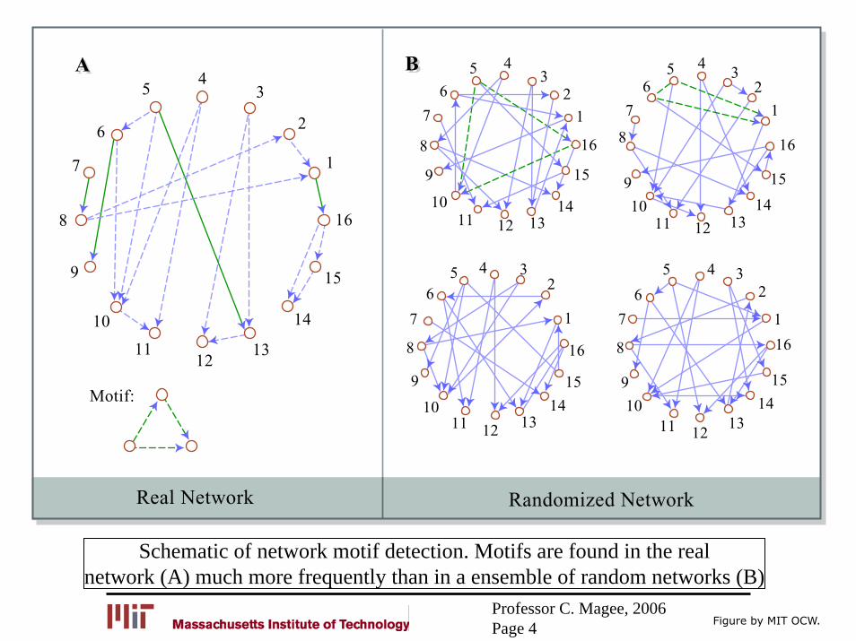
• Milo et al. first extended the concept beyond sociological networks in a 2002 article in Science titled: “Network Motifs: Simple building blocks of Complex Networks”, • They defined motifs in this paper as patterns of
interactions that occur at significantly higher rates in an actual network than in randomized networks and developed an algorithm for extracting them from (directed) networks
Professor C. Magee, 2006Page 4
Schematic of network motif detection. Motifs are found in the realnetwork (A) much more frequently than in a ensemble of random networks (B)
AA BB5
43
2
1
1610
6 65 54 43 3
2 2
1 1
16 16
15 15
14 1413 1312 12
11 1110 10
9 9
7 7
8 8
11 12 1314
15
16
12
5 43
2
1
16
15
14131211
10
9
8
7
63
45
6
7
8
9
15
14
1312
11
Motif:
10
Real Network Randomized Network
9
8
7
6
Figure by MIT OCW.
Professor C. Magee, 2006Page 5
Motifs b
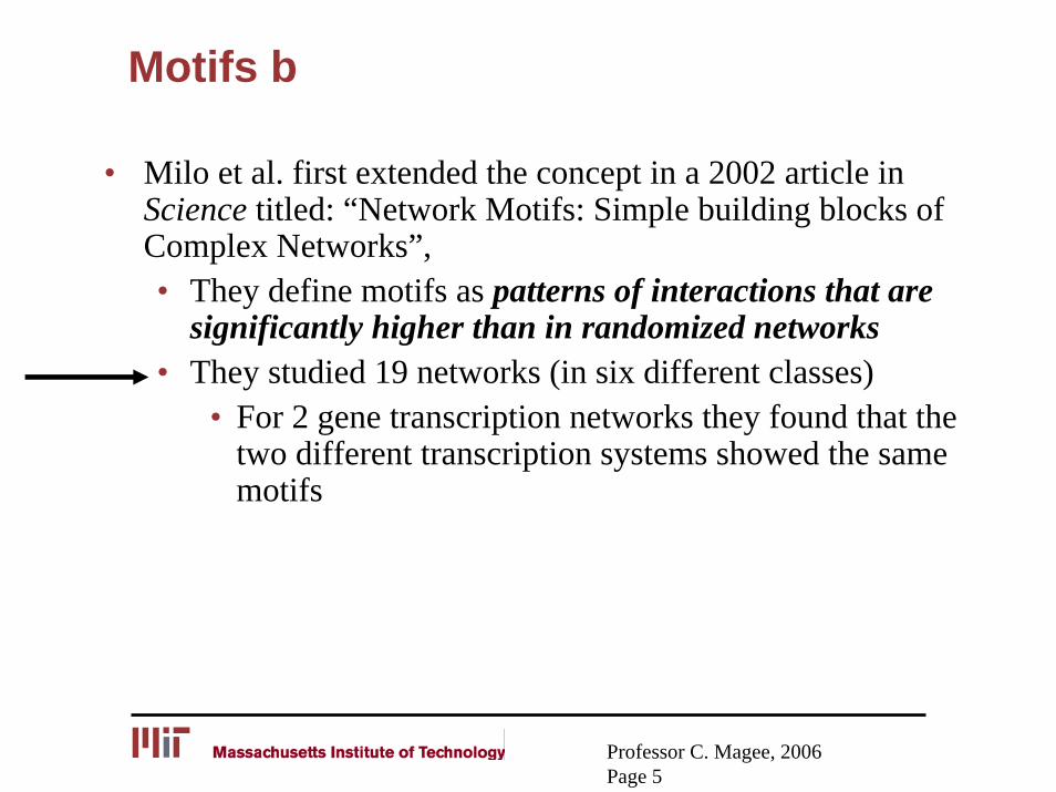
• Milo et al. first extended the concept in a 2002 article in Science titled: “Network Motifs: Simple building blocks of Complex Networks”, • They define motifs as patterns of interactions that are
significantly higher than in randomized networks• They studied 19 networks (in six different classes)
• For 2 gene transcription networks they found that the two different transcription systems showed the same motifs
Professor C. Magee, 2006Page 6
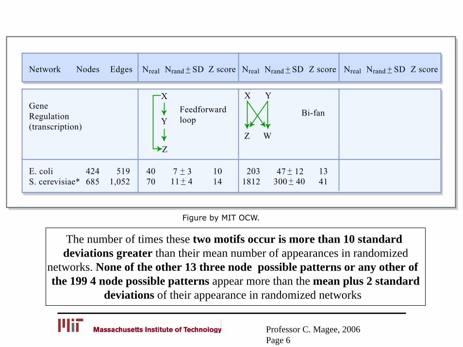
The number of times these two motifs occur is more than 10 standard deviations greater than their mean number of appearances in randomized
networks. None of the other 13 three node possible patterns or any other of the 199 4 node possible patterns appear more than the mean plus 2 standard
deviations of their appearance in randomized networks
Figure by MIT OCW.
Network
Gene Regulation (transcription)
Feedforward loop
Bi-fan
E. coliS. cerevisiae*
424685
5191,052
4070
1014
Nodes Edges Nreal
X
Y
Z
Z
X Y
W
Nrand Z scoreSD+_ Nreal Nrand Z scoreSD+_ Nreal Nrand Z scoreSD+_
7 3+_11 4+_
2031812
1341
47 12+_300 40+_
Professor C. Magee, 2006Page 7
0
0.005
0.01
Con
cent
rati
on o
f F
eedf
orw
ard
Loo
p
0.015
150
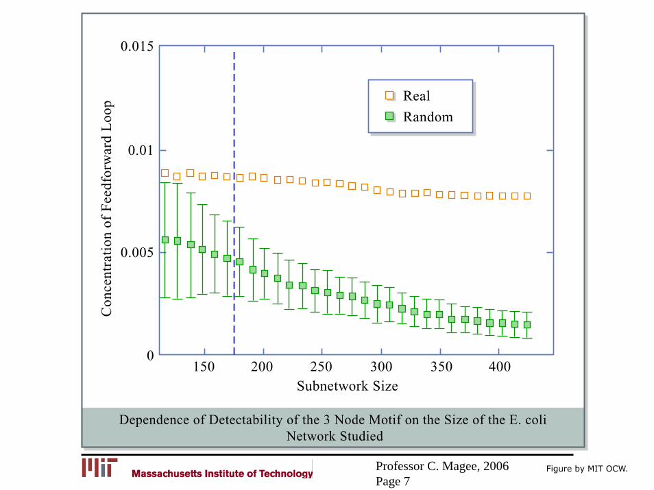
Dependence of Detectability of the 3 Node Motif on the Size of the E. coli Network Studied
200 250Subnetwork Size
300 350 400
Real
Random
Figure by MIT OCW.
Professor C. Magee, 2006Page 8
Motifs c
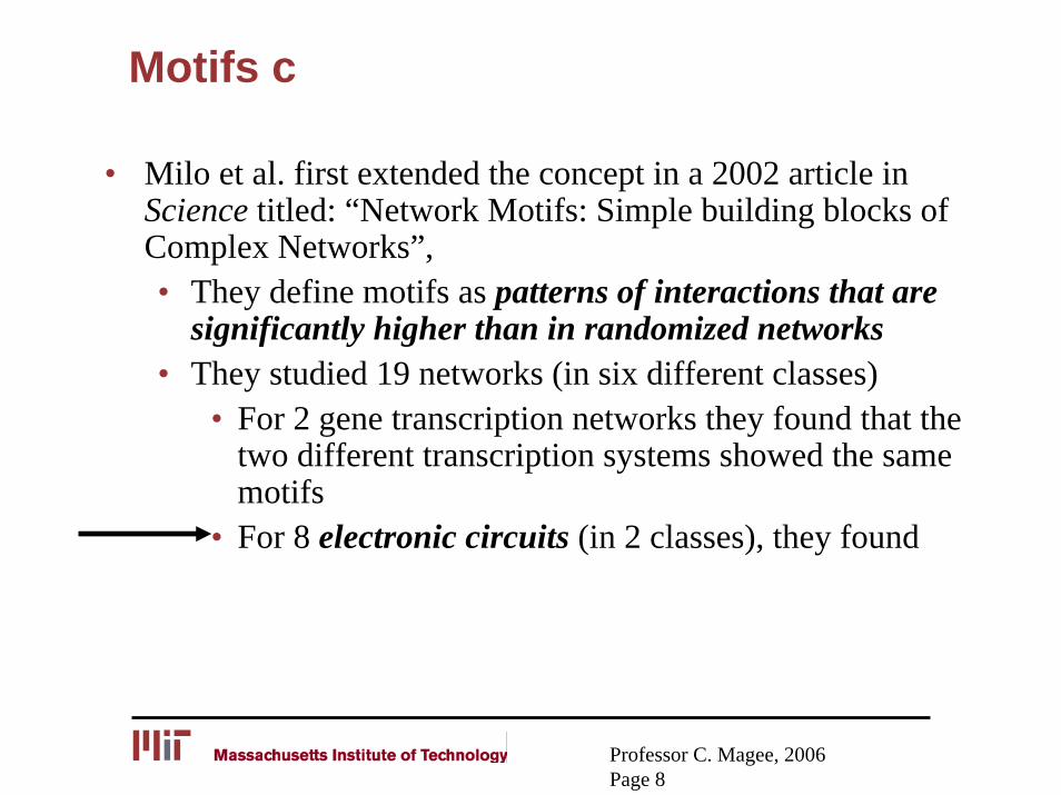
• Milo et al. first extended the concept in a 2002 article in Science titled: “Network Motifs: Simple building blocks of Complex Networks”, • They define motifs as patterns of interactions that are
significantly higher than in randomized networks• They studied 19 networks (in six different classes)
• For 2 gene transcription networks they found that the two different transcription systems showed the same motifs
• For 8 electronic circuits (in 2 classes), they found
Professor C. Magee, 2006Page 9
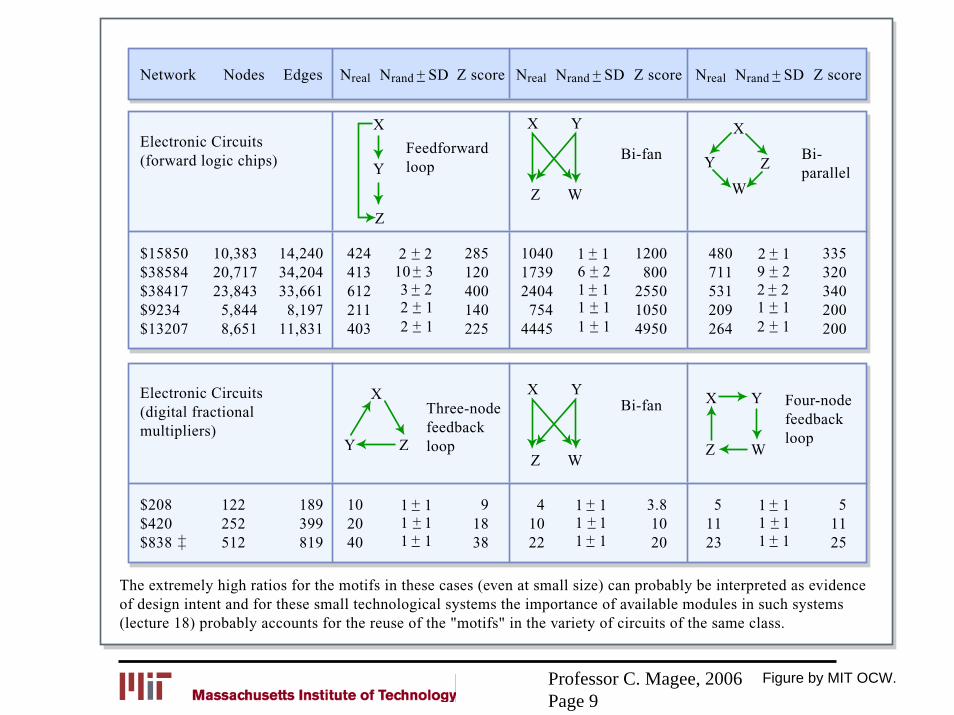
Network
Electronic Circuits(forward logic chips)
Feedforward loop
Bi-fan Bi-parallel
$15850$38584$38417$9234$13207
10,38320,71723,843
5,8448,651
14,24034,20433,661
8,19711,831
424413612211403
285120400140225
Nodes Edges Nreal
X
Y
Z
Z
X Y
W
Nrand Z scoreSD+_ Nreal Nrand Z scoreSD+_ Nreal Nrand Z scoreSD+_
2 2+_10 3+_3 2+_2 1+_2 1+_
104017392404
7544445
1200800
255010504950
1 1+_6 2+_1 1+_1 1+_1 1+_
480711531209264
335320340200200
2 1+_9 2+_2 2+_1 1+_2 1+_
Electronic Circuits(digital fractional multipliers)
Three-node feedbackloop
Bi-fan Four-node feedbackloop
$208$420$838 ++
122252512
The extremely high ratios for the motifs in these cases (even at small size) can probably be interpreted as evidence of design intent and for these small technological systems the importance of available modules in such systems (lecture 18) probably accounts for the reuse of the "motifs" in the variety of circuits of the same class.
189399819
102040
91838
1 1+_1 1+_1 1+_
1 1+_1 1+_1 1+_
1 1+_1 1+_1 1+_
41022
3.81020
51123
51125
X
Y Z
W
X
Y ZZ
X Y
W
X Y
Z W
Figure by MIT OCW.
Professor C. Magee, 2006Page 9
The extremely high ratios for the motifs in these cases (even at smallsize) can probably be interpreted as evidence of design intent andfor these small technological systems the importance of availablemodules in such systems (lecture 18) probably accounts for the
reuse of the same “motifs” in the variety of circuits of the same class.
Professor C. Magee, 2006Page 10
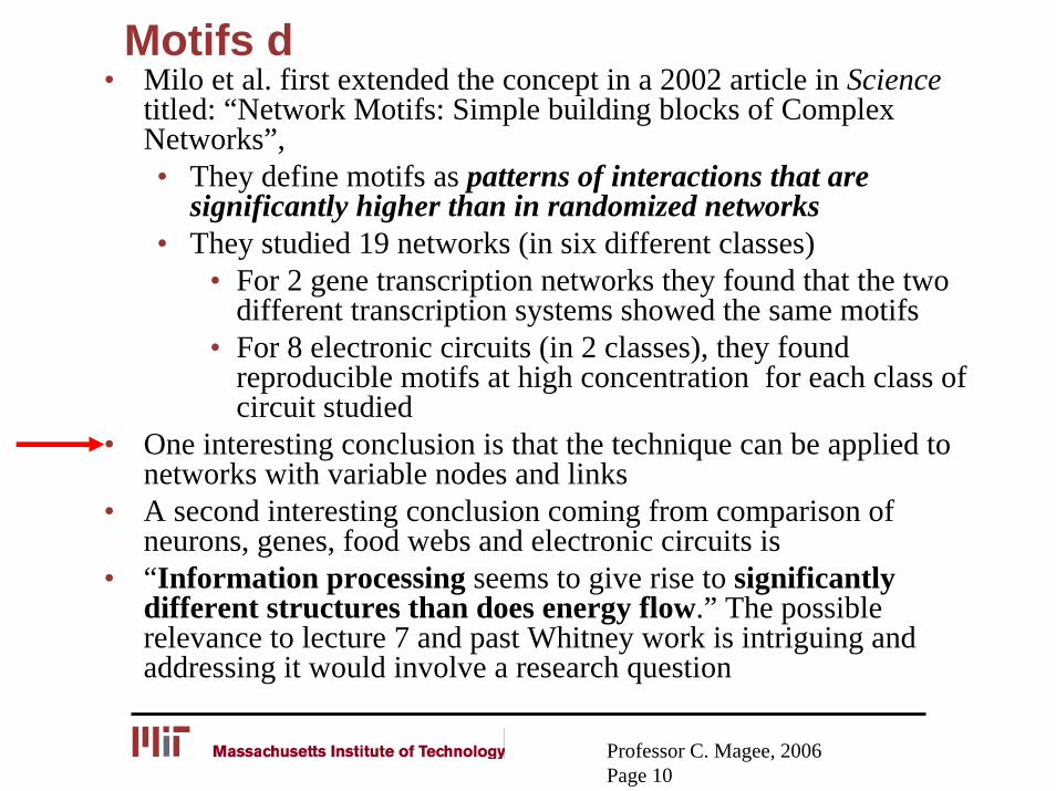
Motifs d• Milo et al. first extended the concept in a 2002 article in Science
titled: “Network Motifs: Simple building blocks of Complex Networks”, • They define motifs as patterns of interactions that are
significantly higher than in randomized networks• They studied 19 networks (in six different classes)
• For 2 gene transcription networks they found that the two different transcription systems showed the same motifs
• For 8 electronic circuits (in 2 classes), they found reproducible motifs at high concentration for each class of circuit studied
• One interesting conclusion is that the technique can be applied to networks with variable nodes and links
• A second interesting conclusion coming from comparison of neurons, genes, food webs and electronic circuits is
• “Information processing seems to give rise to significantly different structures than does energy flow.” The possible relevance to lecture 7 and past Whitney work is intriguing and addressing it would involve a research question
Professor C. Magee, 2006Page 11
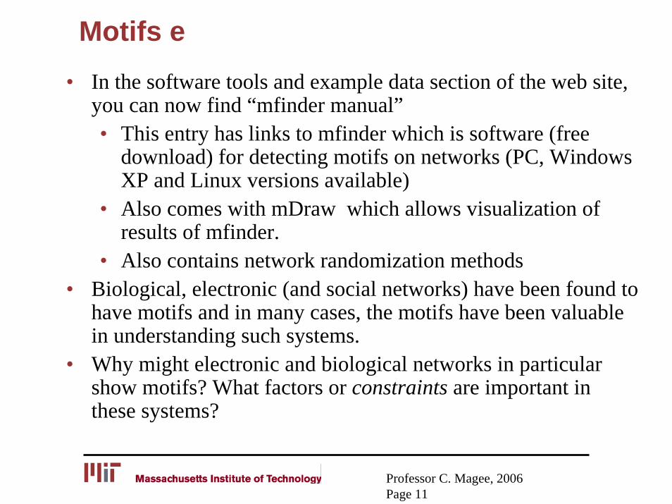
Motifs e• In the software tools and example data section of the web site,
you can now find “mfinder manual”• This entry has links to mfinder which is software (free
download) for detecting motifs on networks (PC, Windows XP and Linux versions available)
• Also comes with mDraw which allows visualization of results of mfinder.
• Also contains network randomization methods• Biological, electronic (and social networks) have been found to
have motifs and in many cases, the motifs have been valuable in understanding such systems.
• Why might electronic and biological networks in particular show motifs? What factors or constraints are important in these systems?
Professor C. Magee, 2006Page 12
Function on a local scale
• The motifs shown for the electronic circuits (and the biologicalsystems) seem to show evidence of functionality imbedded within the network and pursuing a hierarchy of function within technological networks is one interesting avenue suggested by this work.
• The following slides are a brief discussion of an approach used to estimate complexity of various systems attending to hierarchy, interactions and function (Masters thesis of Pierre-Alain Martin)
• After that, we will return to looking at hierarchies of motifs on various levels which is called coarse-graining in the literature (hierarchy of function?)
Professor C. Magee, 2006Page 13
Aspects of Complexity
• Number of elements (scale)• Number of interactions• Patterns of interactions• Number and interaction of hierarchical levels• Scope
• # of functions (and their interactions)• # of time scales (and their interactions)
• Feedback and diverse time delays• # of spatial scales (and their interactions)
• In our “network approximations”, we have deliberately started with the simple end (to do otherwise risks immediate non calculability) and the question is how much complexity must be added for these to be useful in our systems for our purposes.
Professor C. Magee, 2006Page 14
The drivers of Complexity in model and representation discussed
• Number of elements• Number of links (JM idealization)• Number of basic functions (new here)• Hierarchy of these basic functions (new here)
CIPD
Professor C. Magee, 2006Page 15
Functional Classification Matrix
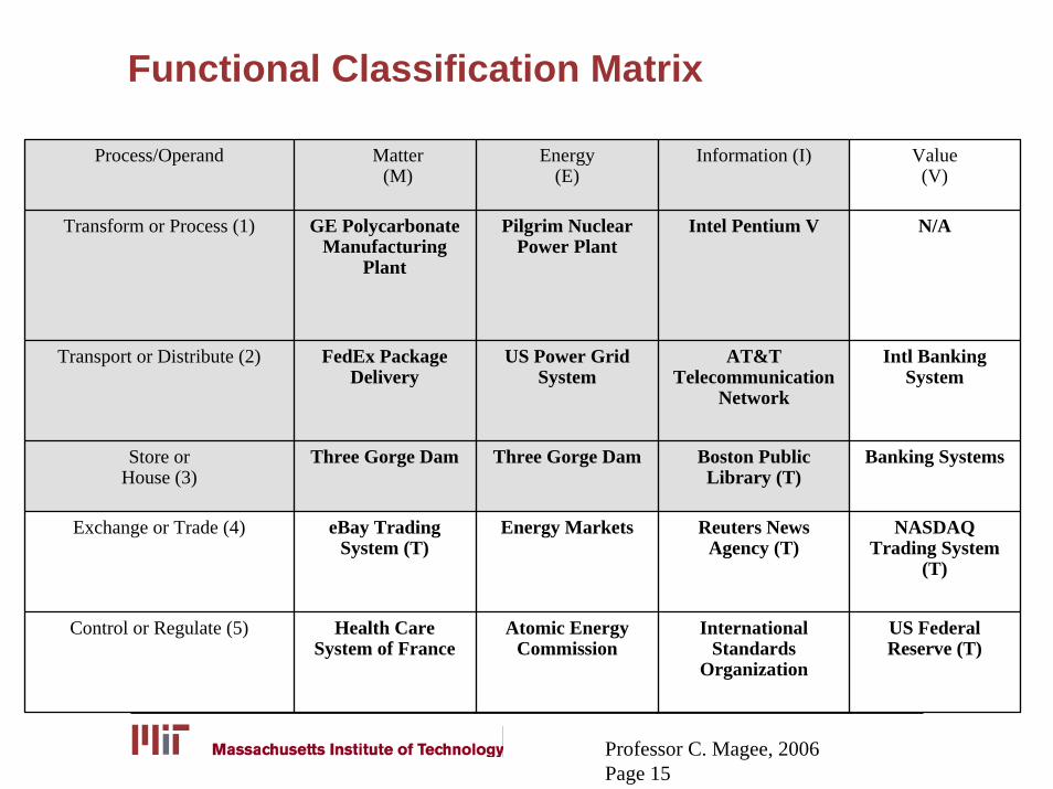
Process/Operand Matter(M)
Energy(E)
Information (I) Value(V)
Transform or Process (1) GE Polycarbonate Manufacturing
Plant
Pilgrim Nuclear Power Plant
Intel Pentium V N/A
Transport or Distribute (2) FedEx Package Delivery
US Power Grid System
AT&T Telecommunication
Network
Intl Banking System
Store orHouse (3)
Three Gorge Dam Three Gorge Dam Boston Public Library (T)
Banking Systems
Exchange or Trade (4) eBay Trading System (T)
Energy Markets Reuters News Agency (T)
NASDAQ Trading System
(T)
Control or Regulate (5) Health Care System of France
Atomic Energy Commission
International Standards
Organization
US Federal Reserve (T)
Professor C. Magee, 2006Page 16
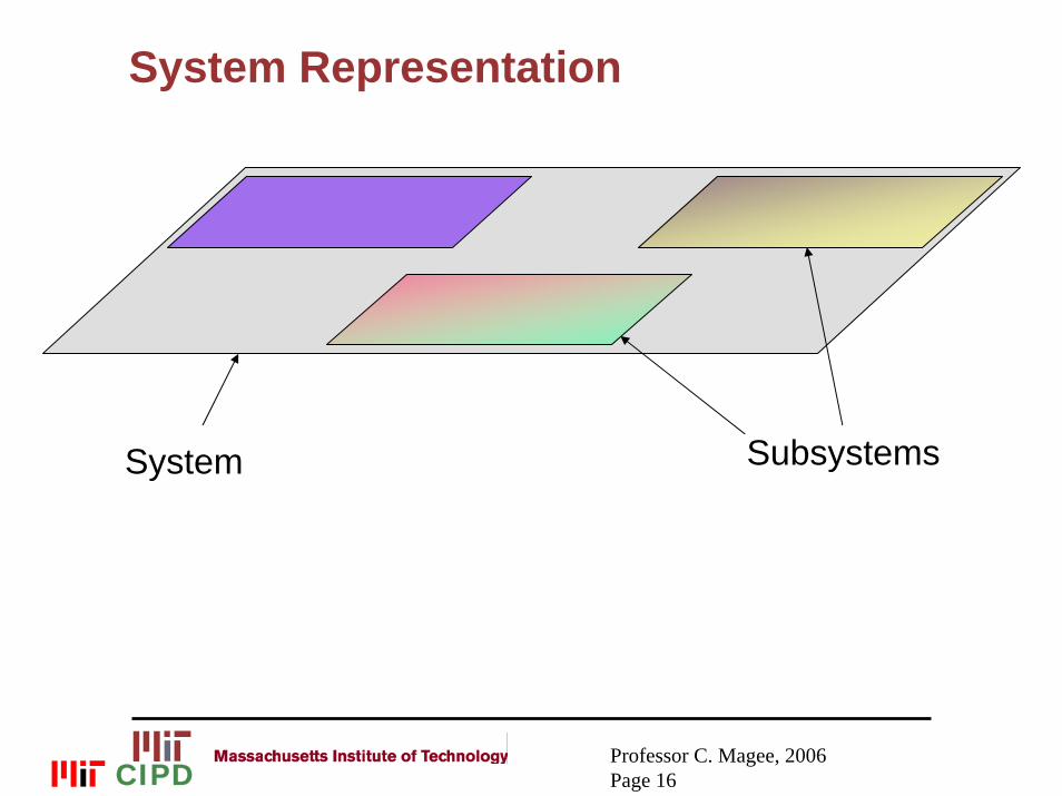
System Representation
System Subsystems
CIPD
Professor C. Magee, 2006Page 17
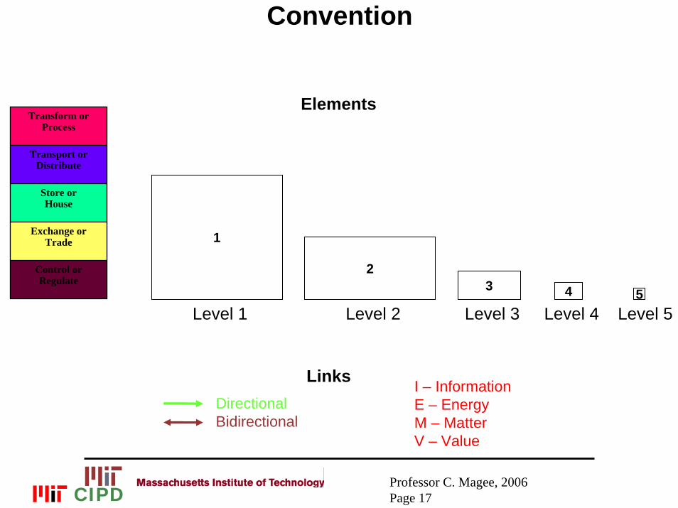
Convention
ElementsTransform or
Process
Transport or Distribute
Store orHouse
Exchange or Trade
Control or Regulate
1
23 4 5
Level 1 Level 2 Level 3 Level 4 Level 5
Links I – Information E – Energy M – Matter V – Value
DirectionalBidirectional
CIPD
Professor C. Magee, 2006Page 18
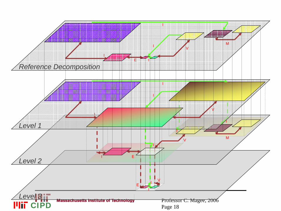
Reference Decomposition
I
M
I
E
I
I
V
Level 3
E I V
I
Level 2
M
IV
I
I
I
I
I
V
Level 1
I E
CIPD
Professor C. Magee, 2006Page 19
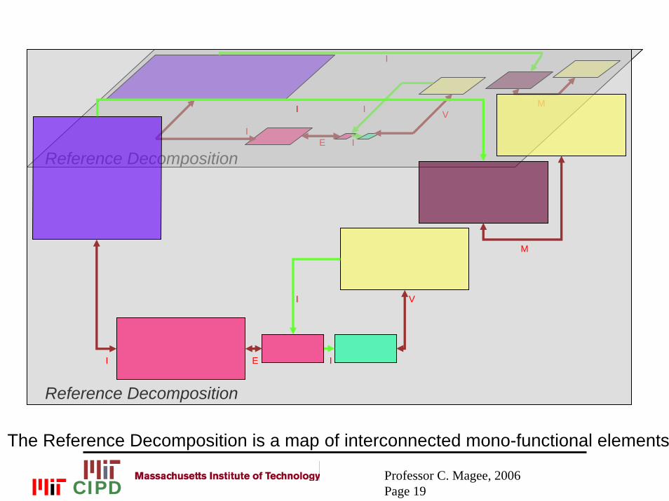
Reference Decomposition
I
M
I
E
I
I
VI
Reference Decomposition
I IE
V
M
I
The Reference Decomposition is a map of interconnected mono-functional elements
CIPD
Professor C. Magee, 2006Page 20
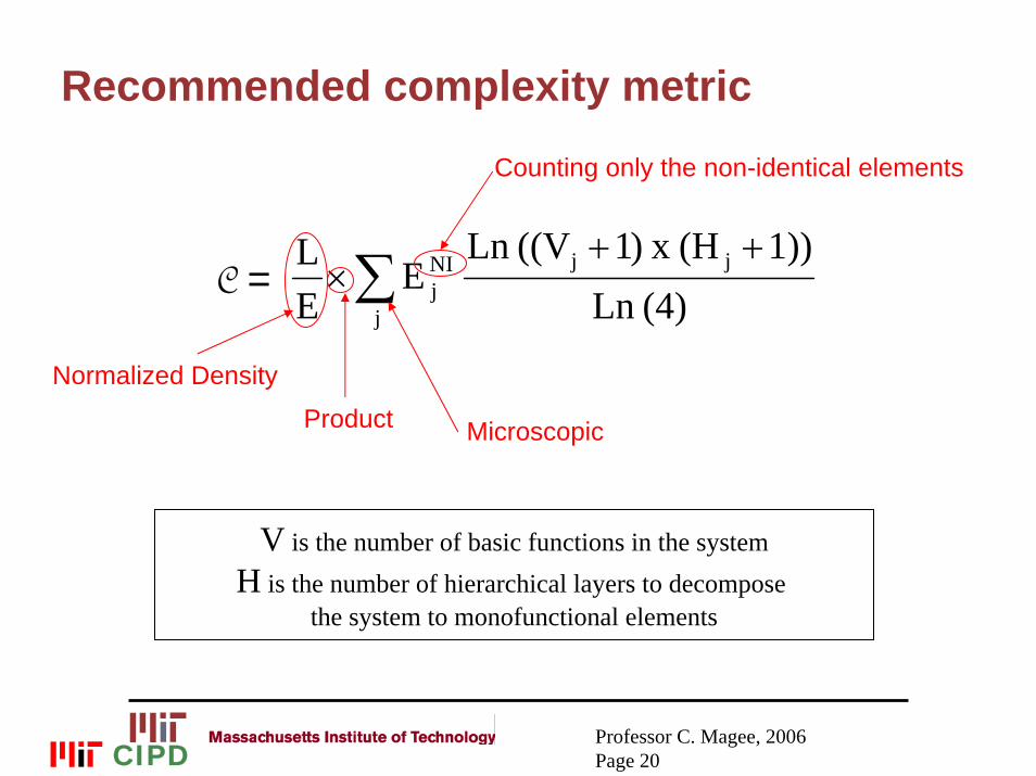
C = (4)Ln
1)) (H x )1((VLn E
EL jj
j
NIj
++×∑
Microscopic
Counting only the non-identical elements
Product
Recommended complexity metric
Normalized Density
V is the number of basic functions in the systemH is the number of hierarchical layers to decompose
the system to monofunctional elements
CIPD
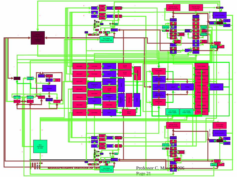
Professor C. Magee, 2006Page 21
RCMSRemote Control
&Monitoring
System
Switch ReceivChrono.
InterfaceBoard
ProcOs
InterfaceBoard
Mixer
DAC
DigitalGener0Switch
Convert
Mixer
MixerConvert
Convert
Aircraft TargetChannel RGN
Weather TargetChannel RGN
Filter
Filter
Switch
Switch
Filter
Filter
Switch
Switch
Switch
Os1Os2
Swi-tch x
Os1Os2
Swi-tch x
PSU-2500SPower Supply Unit
E
I
E
Control
Reflector Feed HornAssembly
WaveguideConnection Fan
E
EM
EncoderA Multi-channel
Transmission EncoderB
I
Power SupplyA
Interface A Interface B
E
I
EPower SupplyB
PowerSupply
Pedestal
I
E
E
E
IE
I
Switch ReceivChrono.
InterfaceBoard
ProcOs
InterfaceBoard
Mixer
DAC
DigitalGener0Switch
Convert
Mixer
MixerConvert
Convert
Aircraft TargetChannel RGN
Weather TargetChannel RGN
Filter
Filter
Switch
Switch
Filter
Filter
Switch
Switch
Switch
Os1Os2
Swi-tch x
Os1Os2
Swi-tch x
PSU-2500SPower Supply Unit
Formatting
Modulus
Interface
Switch
CFAR Threshold
Echo Detection
Phase/Amplit.Compensation
AdaptativeDoppler Filter
InterferenceProcessing
DigitalCompression
Phase/Amplit.CompensationMeasurement
Clutter Map
Voyager
BITE
FanPowerSupply
Aircraft TargetData Processing
Bank Select
Coupler
Driver
Synchronizer
Out
put V
ideo
Output DataFormatting
Output Interface
Formatting
Modulus
Interface
Switch
CFAR Threshold
Echo Detection
Phase/Amplit.Compensation
AdaptativeDoppler Filter
InterferenceProcessing
DigitalCompression
Phase/Amplit.CompensationMeasurement
Clutter Map
InterfaceFormatting
RangeIntegration
Interface
Switch
Max
Ground ClutterFiltering
FilterSelection
Thresholding
InterfaceProcess
PulseCompression
STCCompensation
AnalogousPropagation
Switch
TheoreticalThreshold
Tables
Scan to ScanIntegration
6 Level Filter Selection Map
Switch
Voyager
BITE
FanPowerSupply
Aircraft TargetData Processing
Bank Select
MergeFormat
Coupler
Driver
Synchronizer
Weather DataProcessing
Output Interface
Out
put V
ideo
Switch
Interface &Safety Board B
Interface &Safety Board A
RCMS Interface Board
PreamplifierA
PreamplifierB
Power Module
Divider Combiner
Power Module
Power Module
Power Module
Power Module
Power Module
Power Module
Power ModuleLow VoltagePower Supply
Low VoltagePower Supply
I
EI
I
I
IE
I
E E E
E
E
I
E
Attenuator
Attenuator
Atte
nuat
or
Attenuator
Attenuator
Attenuator
Attenuator
Attenuator
Attenuator
Sw
itch
Switch
Switch
Switch
Converter
Converter
Converter
Dispatcher1->4
Dispatcher1->4
RCVRPROT
RCVRPROT
RCVRPROT
Circulator
Dis
patc
her
1->2
Atte
nuat
or
Sw
itch
Switch
Attenuator
RCVRPROT
I
MainDistribution
AE 2000
I
I
I
I
E
E
I
I
I
I
I
I
I
E
E
E
E
E I
I
I
I
E
ME
I
I I
I
I
I
I II
I
I
I
E
I
I
I
EE
II
I
II
I
I
I
I
I
I
I
I
II
I
I
I
I
I
II
I
II
I
I
I
I
I
I
I
I
I
I
I
I
II
I
I
I
I
III
I
I
I
II
I
II
I
I
I
I
I
I
I
II
I
II
I
II
I
I
I
I
ME
E
I
I
I
E
E
E
E
E
E
E
E
E
E
E
E
I
I
I
EE
E
E E EE
E
EE
E
E
E
E E
E
E
E
E
E
E E
E
E
III
II
I
I
I
I
I
E
E
E
E
I
I
I
IE
I
II
II
I
I
I
I I
I II IIII
III
I
I
I
I
I
E I
I
I
IE
I
I I
I
I
IIII
I
I
I
I
E
I
I
II
I
E
E
E
II
I
I
I II
I
E I
I
E
Professor C. Magee, 2006Page 22
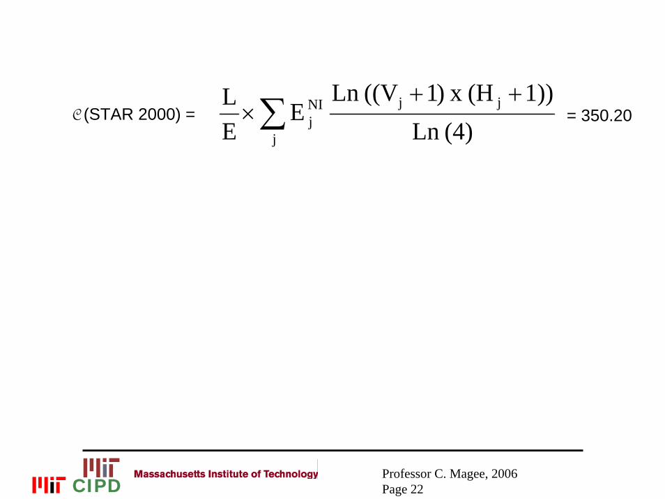
= 350.20(4)Ln
1)) (H x )1((VLn E
EL jj
j
NIj
++×∑C (STAR 2000) =
CIPD
Professor C. Magee, 2006Page 23
Complexity Estimation and Technological System Representation by Networks
• Martin’s thesis work may be a superior way to calculate complexity and worked well for the two cases he studied.
• Much more application to other systems is needed to determine its utility.
• For today’s lecture purpose, we introduce it to allow discussion of node differentiation by function and by hierarchical level. In addition, we want to note the possible utility of the representation developed in that work as a basis for developing more effective (yet tractable) network models for technological systems.
Professor C. Magee, 2006Page 24
Self-similarity and self-dissimilarity
• Wolpert and Macready(2000) introduced the concept of self-dissimilarity as a complexity metric
• They defined self-dissimilarity as “the variability of interaction patterns of a system at different spatio-temporal scales”
• Wolpert and Macready invented relatively elaborate methods for statistically applying their concept and demonstrate it onlythrough numerical simulations.
• Itzkovitz et. al (2004) have recently developed a method they call “coarse-graining” based on their prior work on motifs. This method also assesses self-dissimilarity and has been applied to biological and technological networks.
Professor C. Magee, 2006Page 25
Coarse-Graining
• Itzkovitz et. al. investigate Coarse-Graining as an objective means for “reverse-engineering” that can be applied even when the lower level functional units are unknown (biological focus).
• The coarse-grained version of a network is a new network with fewer elements. This is achieved by replacing some of the original nodes by CGU’s (patterns of node interactions at the level being examined-motifs chosen somewhat differently).
• Itzkovitz et. al. apply simulated annealing to arrive at an optimum set of CGU’s (minimize the “vocabulary” of CGU's and the complexity of the chosen CGU’s while maximizing the coverage of the original network by the coarse-grained description).
Professor C. Magee, 2006Page 26
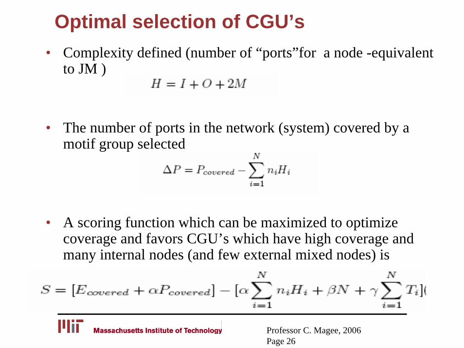
Optimal selection of CGU’s• Complexity defined (number of “ports”for a node -equivalent
to JM )
• The number of ports in the network (system) covered by a motif group selected
• A scoring function which can be maximized to optimize coverage and favors CGU’s which have high coverage and many internal nodes (and few external mixed nodes) is
Professor C. Magee, 2006Page 27
Coarse-Graining
• Itzkovitz et. al. investigate Coarse-Graining as an objective means for “reverse-engineering” that can be applied even when the lower level functional units are unknown (biological focus).
• The coarse-grained version of a network is a new network with fewer elements. This is achieved by replacing some of the original nodes by CGU’s (patterns of node interactions at the level being examined-motifs chosen somewhat differently).
• Itzkovitz et. al. apply simulated annealing to arrive at an optimum set of CGU’s (minimize the “vocabulary” of CGU's and the complexity of the chosen CGU’s while maximizing the coverage of the original network by the coarse-grained description).
• Applying this algorithm to an electronic circuit..
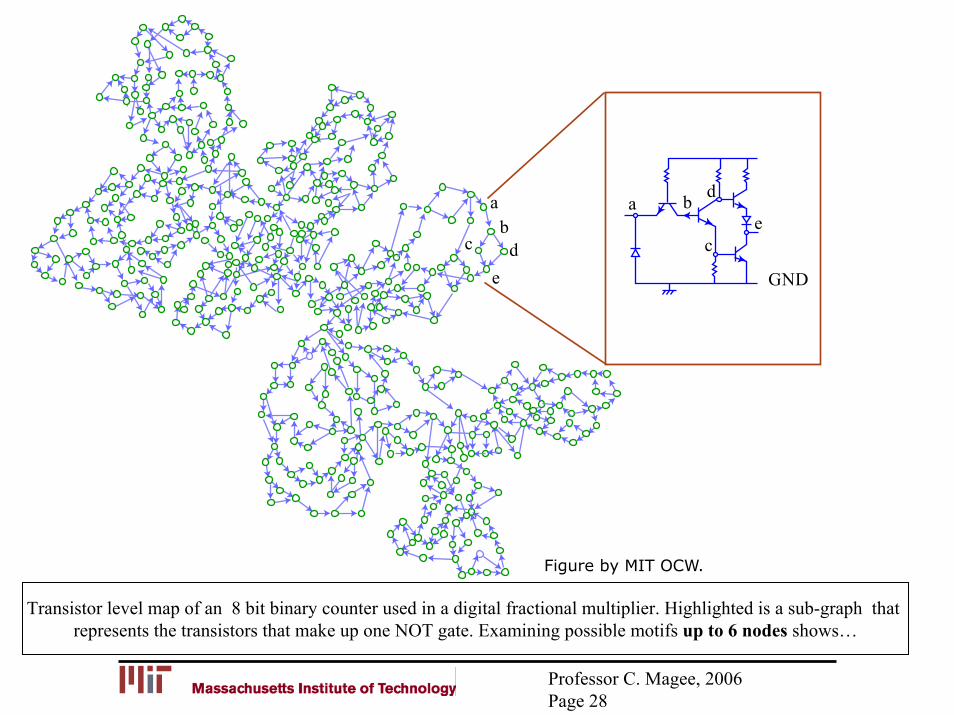
Transistor level map of an 8 bit binary counter used in a digital fractional multiplier. Highlighted is a sub-graph that represents the transistors that make up one NOT gate. Examining possible motifs up to 6 nodes shows…
Professor C. Magee, 2006Page 28
aab
b
c cd
d
e
e
GND
Figure by MIT OCW.
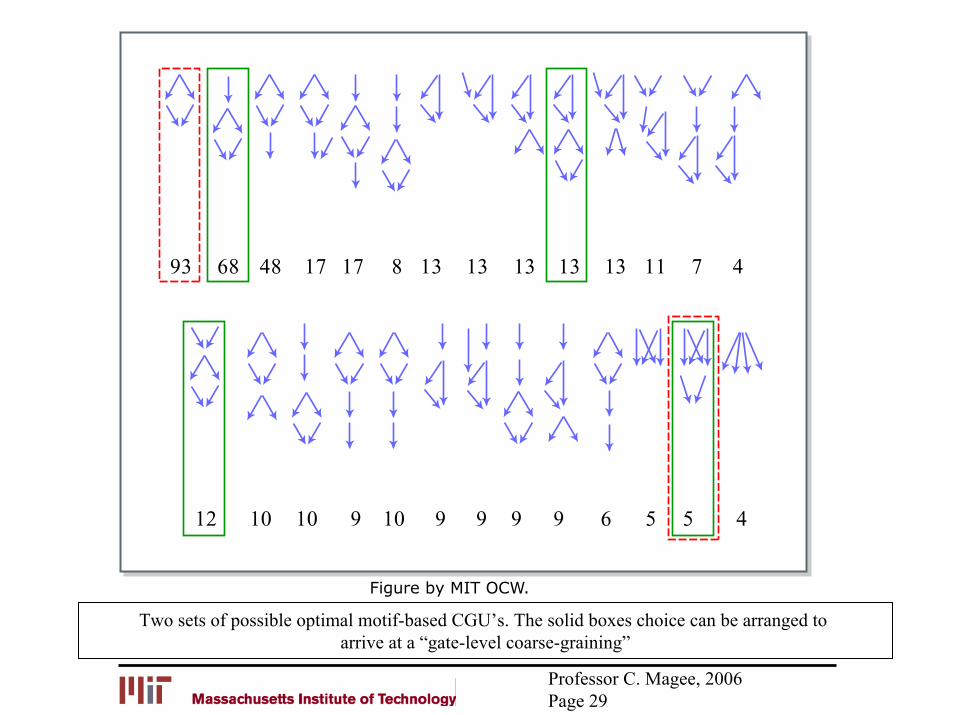
Two sets of possible optimal motif-based CGU’s. The solid boxes choice can be arranged to arrive at a “gate-level coarse-graining”
Professor C. Magee, 2006Page 29
93
12 10 10 10 6 5 5 49 9 9 9 9
68 48 17 17 13 13 13 13 13 11 7 48
Figure by MIT OCW.
Professor C. Magee, 2006Page 30
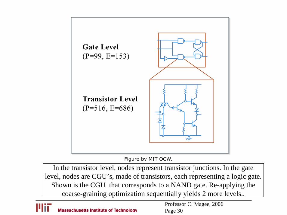
In the transistor level, nodes represent transistor junctions. In the gatelevel, nodes are CGU’s, made of transistors, each representing a logic gate.
Shown is the CGU that corresponds to a NAND gate. Re-applying thecoarse-graining optimization sequentially yields 2 more levels..
Figure by MIT OCW.
Gate Level(P=99, E=153)
Transistor Level(P=516, E=686)
Professor C. Magee, 2006Page 31
CGU 1
D Q
Q
CGU 2
CGU 1
CGU 1
CGU 2
CGU 3
CGU 3
CGU 2CGU 3
CGU 1
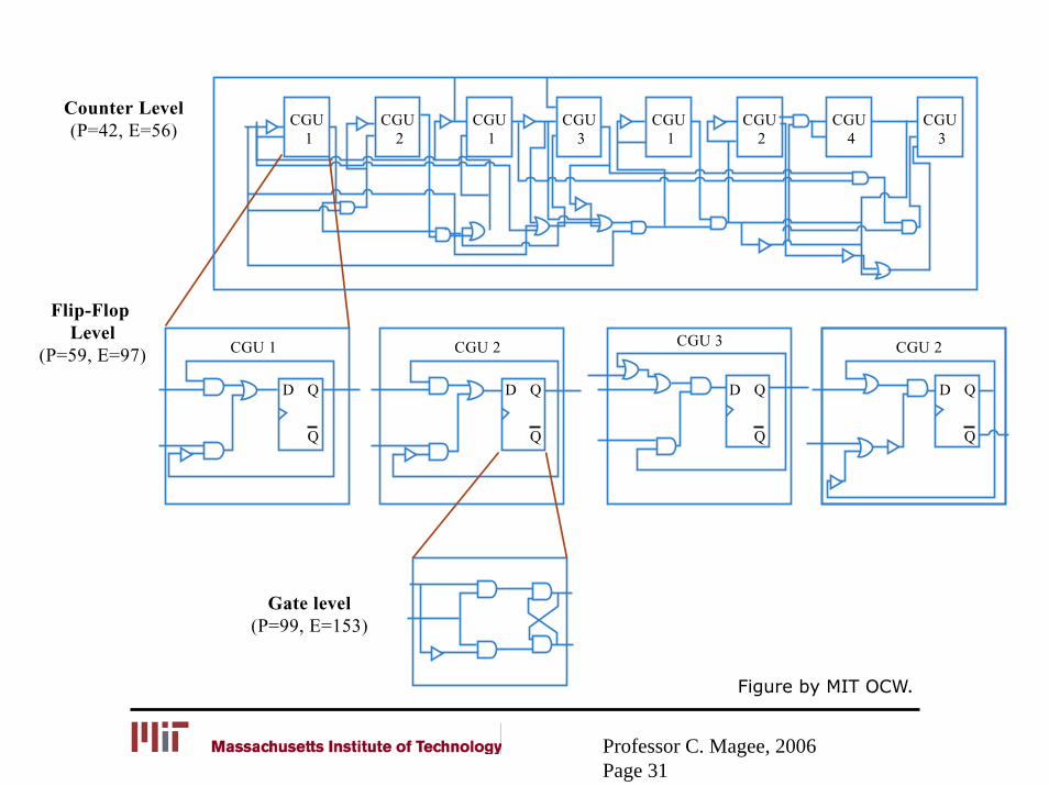
Counter Level(P=42, E=56)
Flip-Flop Level
(P=59, E=97)
Gate level(P=99, E=153)
CGU 2
CGU 4
D Q
Q
D Q
Q
D Q
Q
Figure by MIT OCW.
Professor C. Magee, 2006Page 32
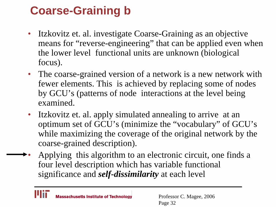
Coarse-Graining b
• Itzkovitz et. al. investigate Coarse-Graining as an objective means for “reverse-engineering” that can be applied even when the lower level functional units are unknown (biological focus).
• The coarse-grained version of a network is a new network with fewer elements. This is achieved by replacing some of nodes by GCU’s (patterns of node interactions at the level being examined.
• Itzkovitz et. al. apply simulated annealing to arrive at an optimum set of GCU’s (minimize the “vocabulary” of GCU’swhile maximizing the coverage of the original network by the coarse-grained description).
• Applying this algorithm to an electronic circuit, one finds a four level description which has variable functional significance and self-dissimilarity at each level
Professor C. Magee, 2006Page 33
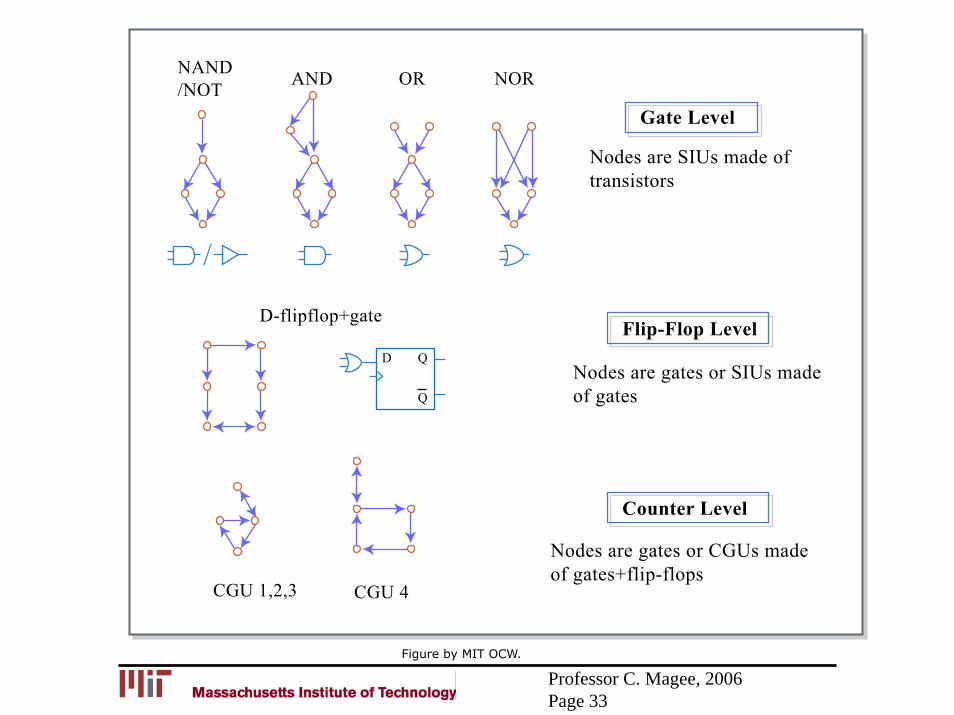
Figure by MIT OCW.
Gate Level
Nodes are SIUs made of transistors
NAND/NOT
D-flipflop+gate
CGU 1,2,3 CGU 4
AND OR NOR
/
Flip-Flop Level
Nodes are gates or SIUs made of gates
Counter Level
Nodes are gates or CGUs madeof gates+flip-flops
D Q
Q
Professor C. Magee, 2006Page 33
Self-dissimilarity at multiple levels in the electronic circuit.This change of patterns with level apparently applies to all
biological and technological networks studied thus far.
Professor C. Magee, 2006Page 34
Coarse-Graining c• Itzkovitz et. al. investigate Coarse-Graining as an objective means
for “reverse-engineering”.• The coarse-grained version of a network is a new network with
fewer elements. • Itzkovitz et. al. apply simulated annealing to arrive at an optimum
set of GCU’s• Applying this algorithm to an electronic circuit, one finds a four
level description which has variable functional significance and self-dissimilarity at each level
• Note the fundamental difference between Coarse-Graining and algorithms for detection of community structure:• Community structure algorithms try to optimally divide networks
into sub-graphs with minimal interconnections but these sub-graphs are distinct and complex
• Coarse-Graining seeks a small dictionary of simple sub-graph types in order to elucidate the function of the network in terms of recurring building blocks
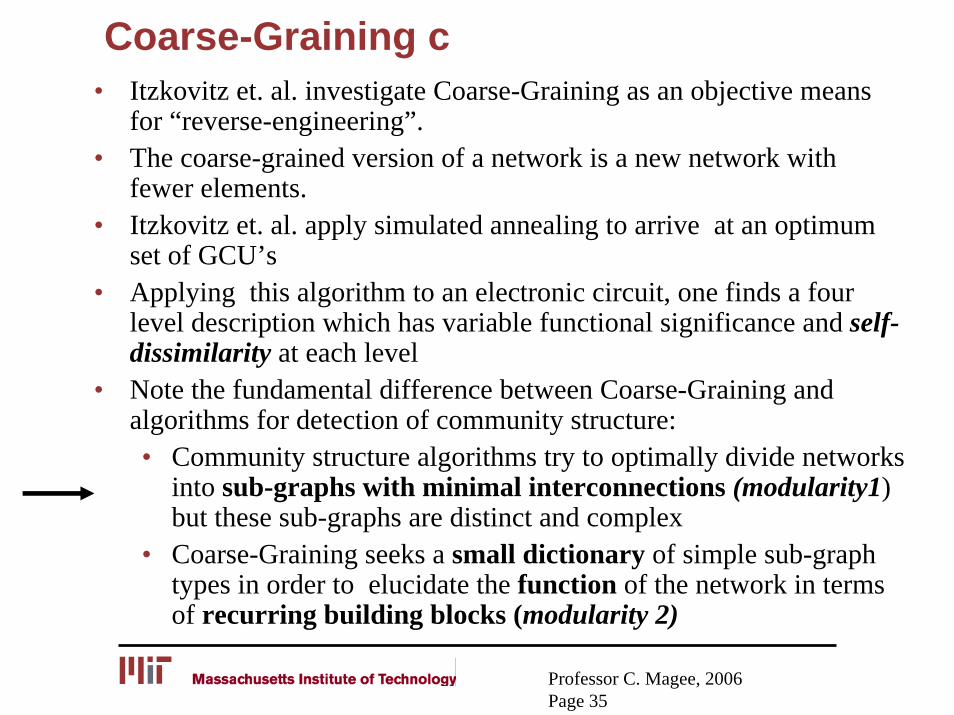
Professor C. Magee, 2006Page 35
Coarse-Graining c• Itzkovitz et. al. investigate Coarse-Graining as an objective means
for “reverse-engineering”.• The coarse-grained version of a network is a new network with
fewer elements. • Itzkovitz et. al. apply simulated annealing to arrive at an optimum
set of GCU’s• Applying this algorithm to an electronic circuit, one finds a four
level description which has variable functional significance and self-dissimilarity at each level
• Note the fundamental difference between Coarse-Graining and algorithms for detection of community structure:• Community structure algorithms try to optimally divide networks
into sub-graphs with minimal interconnections (modularity1) but these sub-graphs are distinct and complex
• Coarse-Graining seeks a small dictionary of simple sub-graph types in order to elucidate the function of the network in terms of recurring building blocks (modularity 2)
Professor C. Magee, 2006Page 36
Different Definitions of “Modular” or “Module” (modified from Whitney)
• You can see different elements and the places where they join (common engineering view particularly in ME but also in economics): H. Simon’s near-decomposability(1962).
• Each item does a specific thing (form-function, genotype-phenotype in a one-to-one relationship) (Suh, Altenberg and also many biological papers discussing modularity)
• You need only know how to use them and don’t need to know what’s inside (common engineering view particularly in EE and software)
• Interconnectedness is concentrated inside them (Alexander, software design)
• Their links to the outside are standardized , or simple and few (Alexander)
• Modules can be replaced in a system arbitrarily preserving (but possibly modifying) function: (Plug and Play intuition)
Professor C. Magee, 2006Page 37
Different Definitions of “Modular” or “Module”
• You can see different elements and the places where they join (modularity 1)
• Each item does a specific thing (form-function, genotype-phenotype in a one-to-one relationship) (Suh, Altenberg) (modularity 2)
• You need only know how to use them and don’t need to know what’s inside (modularity 2)
• Interconnectedness is concentrated inside them (Alexander)(software design) (modularity 1)
• Their links to the outside are standardized (modularity 2), or simple and few (Alexander) (modularity 1)
Professor C. Magee, 2006Page 38
“Better” Definition(s) of Modularity• Modularity 1:
• The system can be decomposed into subunits to arbitrary depth• These subunits can be dealt with separately (to some degree)
• In different domains, such as design, manufacturing, use, error-correction, recycling
• Modularity 2:• The functions of the system can be associated with clusters of
physical elements• in the limit one function:one module
• These elements operate (somewhat) independently• (They do not have to be physically contiguous)
• Merged definition• The intuitive “Plug and Play” requires both definitions to be
operable (without qualifications in brackets)• There are physical constraints in moderately higher power systems that
prevent modularity without significant qualification (Whitney)
Professor C. Magee, 2006Page 39
Coarse-Graining d• Itzkovitz et. al. investigate Coarse-Graining as an objective
means for “reverse-engineering”.• The coarse-grained version of a network is a new network with
fewer elements. • Itzkovitz et. al. apply simulated annealing to arrive at an
optimum set of GCU’s• Applying this algorithm to an electronic circuit, one finds a
four level description which has variable functional significance and self-dissimilarity at each level
• Note the fundamental difference between Coarse-Graining and algorithms for detection of community structure
• Note that motifs and coarse-graining have thus far only been applied to fairly simple technological systems• Monofunctional from the Martin-Magee perspective and
easily functionally modularized
Professor C. Magee, 2006Page 40
Research Questions• Should we apply community structure separation and coarse-
graining at different levels for improved understanding (and design?) of complex technological (and biological) systems?
• Does the form-function relationship only work for relatively simple systems?
• To what degree, do the two kinds of modularity apply to different levels of abstraction and/or power/information differences?
• Hypotheses:• For a truly complex system, one has multiple functions that
cannot be separately decomposed.• For such a system, one might decompose (sequentially) by
community structure (interaction density) to the level of mono-functionality (Martin-Magee representation arrived at objectively)
• One then could examine the resulting mono-functional systems by coarse-graining looking for more basic form-function relationships
Professor C. Magee, 2006Page 41
Self-similarity and self-dissimilarity b• Wolpert and Macready(2000) introduced the concept of self-
dissimilarity as a complexity metric• Self-dissimilarity is defined as “the variability of interaction
patterns of a system at different spatio-temporal scales”• Note that as defined this definition is in a sense counter to the
notion (often loosely defined) of “scale free” which implies (at least seems to) the notion that structure is repetitive at various scales
• Wolpert and Macready invented relatively elaborate methods for statistically applying their concept and demonstrate it onlythrough numerical simulations
• Itzkovitz et. al (2004) have recently developed a method they call “coarse-graining” based on their prior work on motifs. This method also assesses self-dissimilarity and has been applied to biological and technological networks.
Professor C. Magee, 2006Page 42
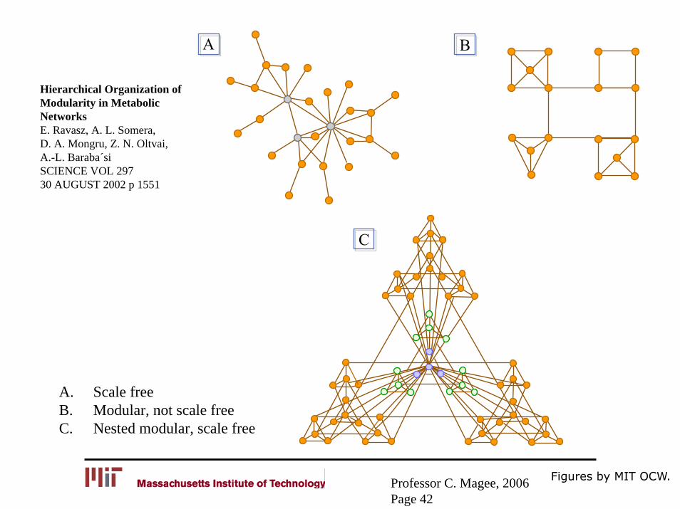
Hierarchical Organization ofModularity in MetabolicNetworksE. Ravasz, A. L. Somera, D. A. Mongru, Z. N. Oltvai,A.-L. Baraba´siSCIENCE VOL 297 30 AUGUST 2002 p 1551
A. Scale freeB. Modular, not scale freeC. Nested modular, scale free
A
C
B
Figures by MIT OCW.
Professor C. Magee, 2006Page 43
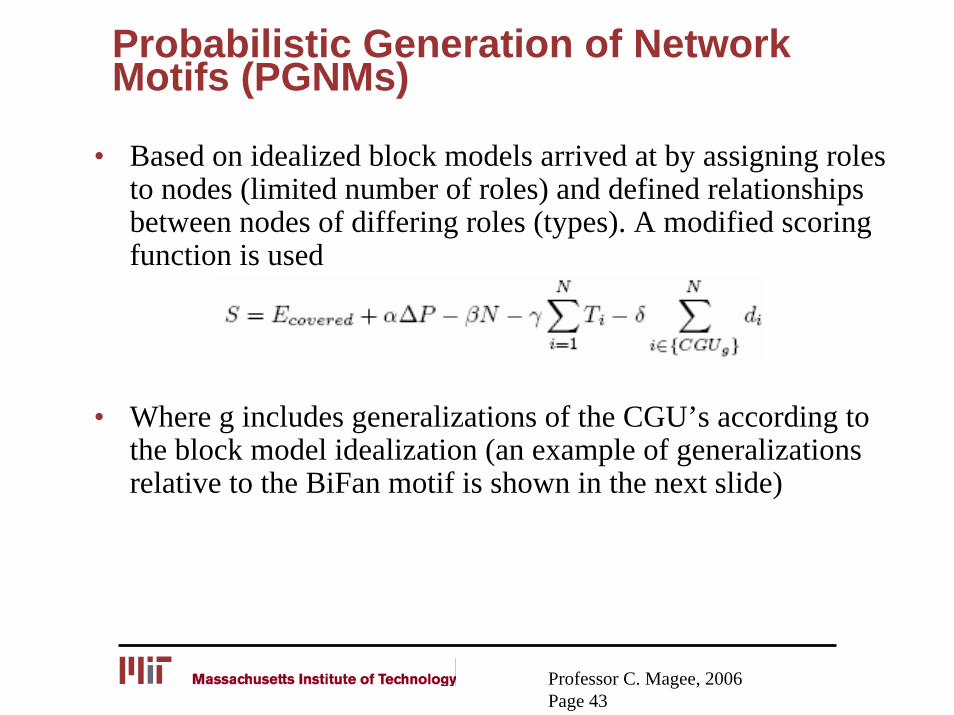
Probabilistic Generation of Network Motifs (PGNMs)
• Based on idealized block models arrived at by assigning roles to nodes (limited number of roles) and defined relationships between nodes of differing roles (types). A modified scoring function is used
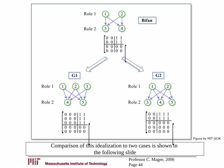
• Where g includes generalizations of the CGU’s according to the block model idealization (an example of generalizations relative to the BiFan motif is shown in the next slide)
Professor C. Magee, 2006Page 44
Comparison of this idealization to two cases is shown in the following slide
1Role 1
Bifan
Role 2
0 00 00 00 0
1 11 10 00 0
[ [
2
3 4
1 2 3Role 1
Role 2
Role 1
Role 2
0 00 00 00 0
1 11 10 00 0
00 0 1 10
000
[ [4 5 3 4 5
1 2
0 10 00 00 0
1 10 00 00 0
00 1 1 10
000
[ [G1 G2
Figure by MIT OCW.
Professor C. Magee, 2006Page 45
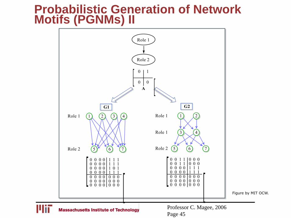
Probabilistic Generation of Network Motifs (PGNMs) II
Figure by MIT OCW.
Role 1
A
Role 2
0
0
1
0[ [1 2 3 4Role 1
Role 2
Role 1
Role 1
Role 2
0 00 00 00 0
1 01 10 00 0
00 0 1 1
1100
0 0 0
11 1 1
00 0
0000
000
000
0 0 00[ [ 0 0
0 00 00 0
1 11 10 00 0
00 1 0 0
1100
0 0 0
00 0 0
00 1
0000
110
000
0 0 00[ [
5 6 7
1 2
3 4
5 6 7
G1 G2
Professor C. Magee, 2006Page 46
Self-similarity and self-dissimilarity c• The scale-free modular example is self-similar.• However, the electronic circuits and biological systems studied
by Itzkovitz et. al are not scale free in that even though the modules are consistent with one another at a given scale, the patterns are dissimilar (in the Wolpert/Macready sense) at different scales (or levels of agglomeration)
• Note that the electronic circuit systems shown to be “scale-rich” by Itzkovitz et. al. show power law degree relationships so the use of the term “scale-free” when power laws is observed is nonsensical. The lack of correlation between structure and power laws was mentioned in lecture 6.
• Li et. al and Doyle et al have introduced the phrase “scale-rich” partly in response to the work by Itzkovitz and have developed some other metrics (related to degree correlation, r)and we will return to this theme in a later discussion of modelsof the Internet
Professor C. Magee, 2006Page 47
References
• 1. R. Milo, S. Shen-Orr, S. Itzkovitz, N. Kashtan, D. Chklovskii, U. Alon, “Network Motifs: Simple building blocks of Complex Networks”, Science, Vol. 298, pp 824-827, (2002)
• 2. Pierre-Alain Martin, “A Framework for Quantifying Complexity and Understanding its Sources: Application to two Large-Scale Systems” SM thesis, MIT, 2004.
• 3. D. H. Wolpert and W. Macready, “Self-dissimilarity: An empirically observable complexity Metric”, Unifying themes in complex systems, New England Complex Systems Institute(2000). A second paper found on the NASA Moffetweb site has similar information and is titled “Self-dissimilarity as a high dimension complexity measure” (2004?)
• 4. S. Itzkovitz, R. Levitt, N. Kashtan, R. Milo, M. Itzkovitz and U. Alon, “Coarse-Graining and Self-Dissimilarity of Complex Networks”, (Oct. 2004)
Recommended