From the Single Component Safety Factor to the
System Reliability Rating The Reliability Concept: A New Way to Assess Gears and Gear Drives
Dr. Ing. Ulrich Kissling, KISSsoft AG
Dr. Ing. Michael Stangl, KISSsoft AG
Dr. Ing. Inho Bae, KISSsoft AG
Introduction
Today, proofs of system reliability for plant components such as gear units or complete mechanical systems
are in increasing demand in various sectors of the power transmission industry. However, there has been no
common language to interpret the reliability for each component, for example, gear engineers prefer the term
‘safety factor’ while bearing engineers use the service life. A component's safety factor or its calculated
service life is actually nothing else than a statement of its reliability. Determining the reliability of individual
parts makes it easier to ascertain the reliability of the mechanical system as a whole.
Stating a system's reliability is also more comprehensible than listing safety factors for those people without
detailed knowledge in mechanical engineering. A statement such as "the probability that gear unit X will fail
during its guaranteed service life of 50,000 hours is less than 0.02%." is much easier to understand than "the
safety factors of all the gears in gear unit X, calculated for an operating time of 50,000 hours, are all bigger
than 1.6.", although both statements mean the same thing.
This paper describes how the probability of failure of the basic gearbox components (shafts, bearings, gears)
can be derived from the component’s service life as specified in the standards, according to the Weibull
failure criterion. In order to determine system reliability, the gear unit elements are classified according to
their significance: if an element fails, does it directly cause the failure of the entire gear unit? Or are
redundancies present? The total reliability of the entire system can then be determined by mathematically
combining the reliability of the individual components. This method can be applied to all ISO-, DIN- or
AGMA-standard calculations that use S-N curves (Woehler lines), either with nominal loads or with load
spectra.
1 Calculating the strength of mechanical components
For many years – and increasingly, since the beginning of the 20th century − engineers have striven to
develop rules for analyzing the strength of elements used in mechanical engineering. German engineers in
particular, used different combinations of basic mechanical engineering formulae in the attempt to define
calculation rules for sizing components. This approach has proven to be extremely successful, and is
implemented world-wide today. A clear illustration of its success is that every ISO calculation standard
published to date is based on this principle.
Calculation methods for mechanical parts are usually developed by different specialists working at different
technical institutions. All these strength analysis methods have one thing in common: they determine the
stresses created by the applied loads and then compare these stresses with the permitted stresses.
However, the calculation procedures differ greatly, depending on what type of machine element is involved
(for example bearings, shafts, gears or bolts). It is these differences in the calculation methods that presents
us a problem. One might expect that the safety factor, which is the permissible stress divided by the
occurring stress, would be sufficient. So that a safety factor greater than 1.0 would means that the part is
adequately dimensioned. Unfortunately, this is not the case. For bearings, the service life is determined and
not the safety factor. In a gear calculation according to ISO [4], the safeties for the tooth root and flank are
determined, giving rise to the question which of the two criteria is decisive, and when. In addition, it is
general that different safety factors are recommended, for example, a minimum safety of 1.4 is used for the
tooth root, but a minimum safety of 1.0 is used for the flank. The reason for the different required minimum
safeties is: if a gear tooth breaks, the entire gear unit will immediately fail, and this is not the case if the flank
becomes pitted. When checking the scuffing risk of a gear, a minimum safety of 2.0 is required; this is
because the calculation method is considered to be "not yet sufficiently tested". In other hand, the minimum
safety that must be achieved in shaft calculation according to the FKM method [9] depends on the
component's importance, i.e. the consequences of the shaft breaking. This is obviously a very sensible
approach. The VDI bolt calculation [13] for safety against sliding for bolted parts requires a minimum safety
of between 1.2 and 1.8, depending on the load. And many similar examples could be added to this list. The
conclusion is: depending on the part, "safety factor" is not equal "safety factor".
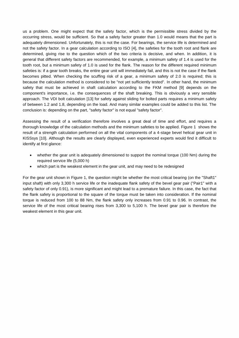
Assessing the result of a verification therefore involves a great deal of time and effort, and requires a
thorough knowledge of the calculation methods and the minimum safeties to be applied. Figure 1 shows the
result of a strength calculation performed on all the vital components of a 4-stage bevel helical gear unit in
KISSsys [10]. Although the results are clearly displayed, even experienced experts would find it difficult to
identify at first glance:
whether the gear unit is adequately dimensioned to support the nominal torque (100 Nm) during the
required service life (5,000 h)
which part is the weakest element in the gear unit, and may need to be redesigned
For the gear unit shown in Figure 1, the question might be whether the most critical bearing (on the "Shaft1"
input shaft) with only 3,300 h service life or the inadequate flank safety of the bevel gear pair ("Pair1" with a
safety factor of only 0.91), is more significant and might lead to a premature failure. In this case, the fact that
the flank safety is proportional to the square of the torque must be taken into consideration. If the nominal
torque is reduced from 100 to 88 Nm, the flank safety only increases from 0.91 to 0.96. In contrast, the
service life of the most critical bearing rises from 3,300 to 5,100 h. The bevel gear pair is therefore the
weakest element in this gear unit.
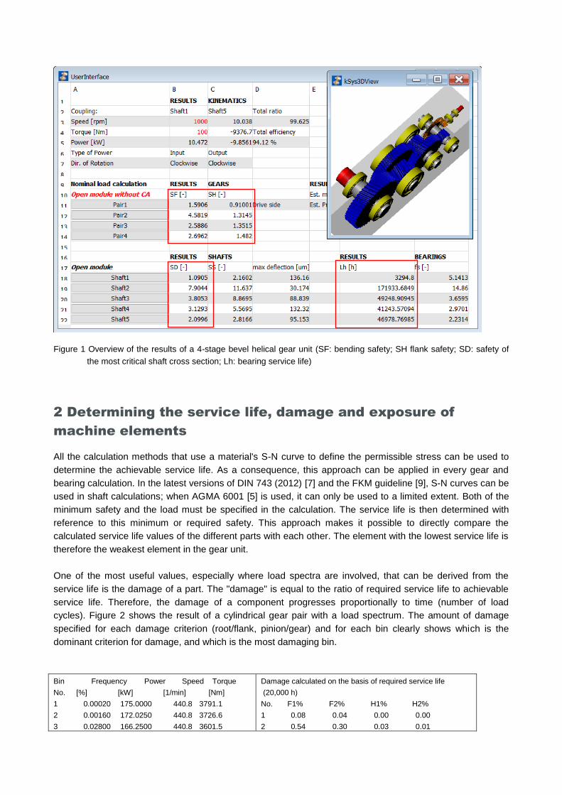
Figure 1 Overview of the results of a 4-stage bevel helical gear unit (SF: bending safety; SH flank safety; SD: safety of
the most critical shaft cross section; Lh: bearing service life)
2 Determining the service life, damage and exposure of
machine elements
All the calculation methods that use a material's S-N curve to define the permissible stress can be used to
determine the achievable service life. As a consequence, this approach can be applied in every gear and
bearing calculation. In the latest versions of DIN 743 (2012) [7] and the FKM guideline [9], S-N curves can be
used in shaft calculations; when AGMA 6001 [5] is used, it can only be used to a limited extent. Both of the
minimum safety and the load must be specified in the calculation. The service life is then determined with
reference to this minimum or required safety. This approach makes it possible to directly compare the
calculated service life values of the different parts with each other. The element with the lowest service life is
therefore the weakest element in the gear unit.
One of the most useful values, especially where load spectra are involved, that can be derived from the
service life is the damage of a part. The "damage" is equal to the ratio of required service life to achievable
service life. Therefore, the damage of a component progresses proportionally to time (number of load
cycles). Figure 2 shows the result of a cylindrical gear pair with a load spectrum. The amount of damage
specified for each damage criterion (root/flank, pinion/gear) and for each bin clearly shows which is the
dominant criterion for damage, and which is the most damaging bin.
Bin Frequency Power Speed Torque
No. [%] [kW] [1/min] [Nm]
1 0.00020 175.0000 440.8 3791.1
2 0.00160 172.0250 440.8 3726.6
3 0.02800 166.2500 440.8 3601.5
Damage calculated on the basis of required service life
(20,000 h)
No. F1% F2% H1% H2%
1 0.08 0.04 0.00 0.00
2 0.54 0.30 0.03 0.01
4 0.27200 158.9000 440.8 3442.3
5 2.00000 150.1500 440.8 3252.7
6 9.20000 141.4000 440.8 3063.2
7 28.00000 132.6500 440.8 2873.6
8 60.49820 123.9000 440.8 2684.1
3 7.25 3.97 0.41 0.12
4 49.86 26.45 3.02 0.87
5 27.25 121.40 9.58 2.54
6 6.35 35.48 16.63 4.41
7 0.00 4.53 17.96 4.77
8 0.00 0.00 13.26 3.52
--------------------------------------------------------------------------
Σ 91.33 192.18 60.89 16.24
Figure 2 Load spectrum (left) and damage displayed per bin for tooth root (F1: pinion, F2: gear) and flank (H1: pinion,
H2: gear). Required service life: 20,000 h. Achievable service life of the gear: 10,400 h (gear tooth root). Therefore, the
total calculated damage is 192%.
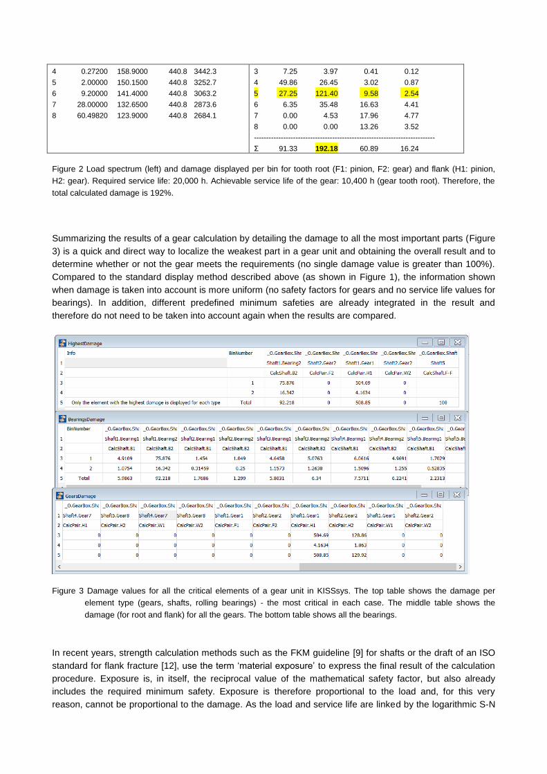
Summarizing the results of a gear calculation by detailing the damage to all the most important parts (Figure
3) is a quick and direct way to localize the weakest part in a gear unit and obtaining the overall result and to
determine whether or not the gear meets the requirements (no single damage value is greater than 100%).
Compared to the standard display method described above (as shown in Figure 1), the information shown
when damage is taken into account is more uniform (no safety factors for gears and no service life values for
bearings). In addition, different predefined minimum safeties are already integrated in the result and
therefore do not need to be taken into account again when the results are compared.
Figure 3 Damage values for all the critical elements of a gear unit in KISSsys. The top table shows the damage per
element type (gears, shafts, rolling bearings) - the most critical in each case. The middle table shows the
damage (for root and flank) for all the gears. The bottom table shows all the bearings.
In recent years, strength calculation methods such as the FKM guideline [9] for shafts or the draft of an ISO
standard for flank fracture [12], use the term ‘material exposure’ to express the final result of the calculation
procedure. Exposure is, in itself, the reciprocal value of the mathematical safety factor, but also already
includes the required minimum safety. Exposure is therefore proportional to the load and, for this very
reason, cannot be proportional to the damage. As the load and service life are linked by the logarithmic S-N
curve, a 10% increase in exposure - depending on the inclination of the S-N curve– will result in an increase
of 100% or more in damage. Only if the results are considered more from a load-oriented viewpoint, the use
of exposure can be given priority over damage and service life.
3 Failure probability of machine elements
The use of damage as a criterion to quantify the reliability of gear unit components (as described above)
would appear to be the ideal method for determining the service life of gear unit components. However, there
is a problem: material properties, such as the S-N curve, are measured by taking samples. The
measurement results scatter. In order to obtain a characteristic value for the calculation, it is usually
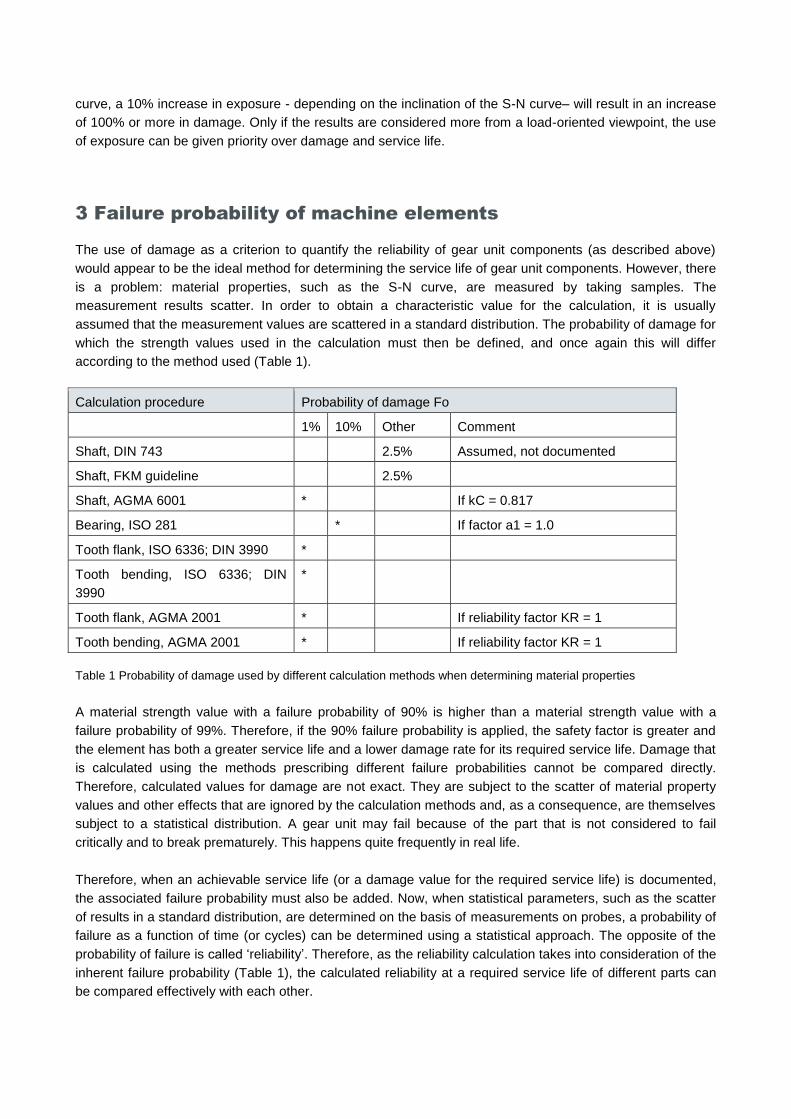
assumed that the measurement values are scattered in a standard distribution. The probability of damage for
which the strength values used in the calculation must then be defined, and once again this will differ
according to the method used (Table 1).
Calculation procedure Probability of damage Fo
1% 10% Other Comment
Shaft, DIN 743 2.5% Assumed, not documented
Shaft, FKM guideline 2.5%
Shaft, AGMA 6001 * If kC = 0.817
Bearing, ISO 281 * If factor a1 = 1.0
Tooth flank, ISO 6336; DIN 3990 *
Tooth bending, ISO 6336; DIN
3990
*
Tooth flank, AGMA 2001 * If reliability factor KR = 1
Tooth bending, AGMA 2001 * If reliability factor KR = 1
Table 1 Probability of damage used by different calculation methods when determining material properties
A material strength value with a failure probability of 90% is higher than a material strength value with a
failure probability of 99%. Therefore, if the 90% failure probability is applied, the safety factor is greater and
the element has both a greater service life and a lower damage rate for its required service life. Damage that
is calculated using the methods prescribing different failure probabilities cannot be compared directly.
Therefore, calculated values for damage are not exact. They are subject to the scatter of material property
values and other effects that are ignored by the calculation methods and, as a consequence, are themselves
subject to a statistical distribution. A gear unit may fail because of the part that is not considered to fail
critically and to break prematurely. This happens quite frequently in real life.
Therefore, when an achievable service life (or a damage value for the required service life) is documented,
the associated failure probability must also be added. Now, when statistical parameters, such as the scatter
of results in a standard distribution, are determined on the basis of measurements on probes, a probability of
failure as a function of time (or cycles) can be determined using a statistical approach. The opposite of the
probability of failure is called ‘reliability’. Therefore, as the reliability calculation takes into consideration of the
inherent failure probability (Table 1), the calculated reliability at a required service life of different parts can
be compared effectively with each other.
Reliability is expressed as a percentage, from 0% to 100%, and psychologically also has an important side-
effect, because safety factors give the impression of being absolute values: a gear unit with high safety
factors cannot fail. In contrast, displaying the same results as reliability, even if it is 99.99%, shows that there
is always an element of uncertainty.
4 Determining the reliability of machine elements
Methods for calculating reliability are still not widely used. However, they gain increasing interest, for
example, in the wind energy sector, where there is a demand for accurately determining system reliability [1].
There are currently no mechanical engineering standards which include this type of rule. A classic source for
this calculation is Bertsche's book [2], in which the possible processes have been described in great detail.
For this reason, the various different methods will not be discussed in this paper. The most commonly used
approach, and one which is well suited to the results that can be achieved in "traditional" mechanical
engineering calculations, is the "Weibull distribution". In this case, Bertsche recommends the use of the 3-
parameter Weibull distribution. The reliability, R, of a machine element is calculated as a function of the
number of load cycles, t, using Equation (1).
𝑅(𝑡) = 𝑒−(
𝑡−𝑡0𝑇−𝑡0
)𝛽
∗ 100% (1)
Parameters T and t0 can be derived from the mathematically achievable service life of the component, Hatt,
as follows (with Fo according to the calculation method from Table 1, β and ftB from Table 2 according to
Bertsche):
𝑇 = (𝐻𝑎𝑡𝑡−𝑓𝑡𝐵∗𝐻𝑎𝑡𝑡10
√−𝑙𝑛(1−𝐹𝑜100
)𝛽 + 𝑓𝑡𝐵 ∗ 𝐻𝑎𝑡𝑡10) ∗ 𝑓𝑎𝑐 (2)
𝑡0 = 𝑓𝑡𝐵 ∗ 𝐻𝑎𝑡𝑡10 ∗ 𝑓𝑎𝑐 (3)
with
𝐻𝑎𝑡𝑡10 =𝐻𝑎𝑡𝑡
(1−𝑓𝑡𝐵) ∗ √𝑙𝑛(1−𝐹𝑜
100)
𝑙𝑛(0,9)+𝑓𝑡𝐵
𝛽 (4)
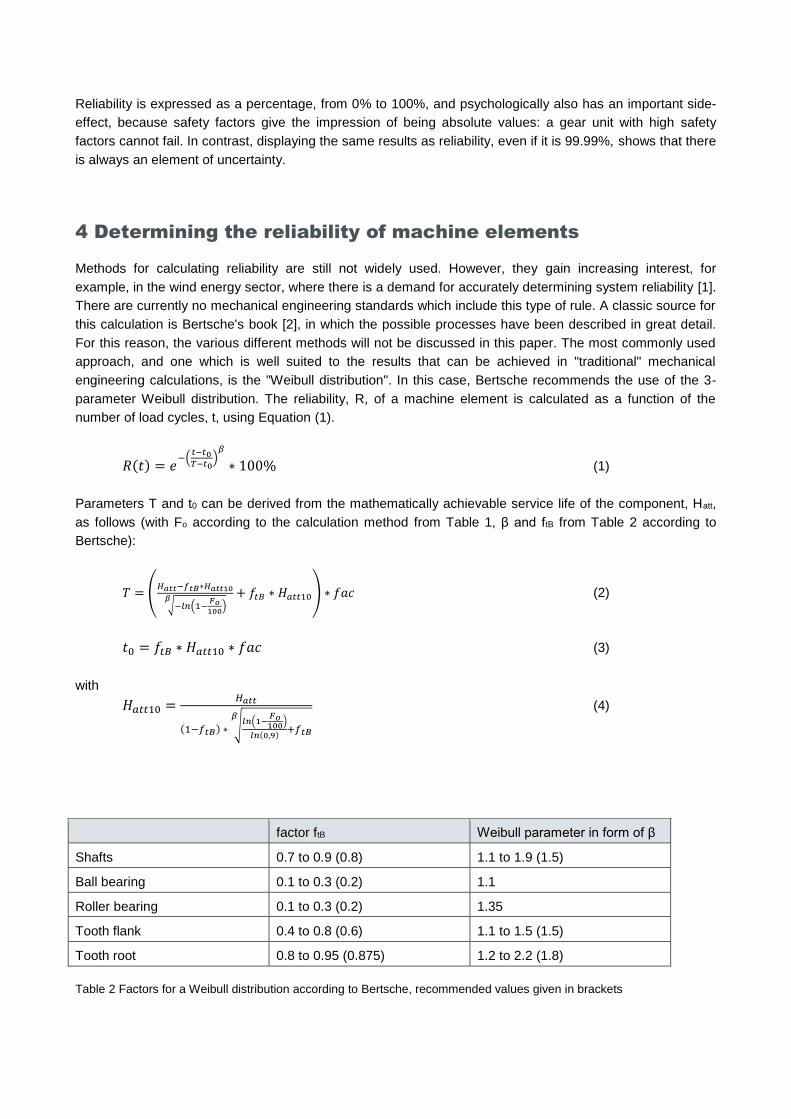
factor ftB Weibull parameter in form of β
Shafts 0.7 to 0.9 (0.8) 1.1 to 1.9 (1.5)
Ball bearing 0.1 to 0.3 (0.2) 1.1
Roller bearing 0.1 to 0.3 (0.2) 1.35
Tooth flank 0.4 to 0.8 (0.6) 1.1 to 1.5 (1.5)
Tooth root 0.8 to 0.95 (0.875) 1.2 to 2.2 (1.8)
Table 2 Factors for a Weibull distribution according to Bertsche, recommended values given in brackets
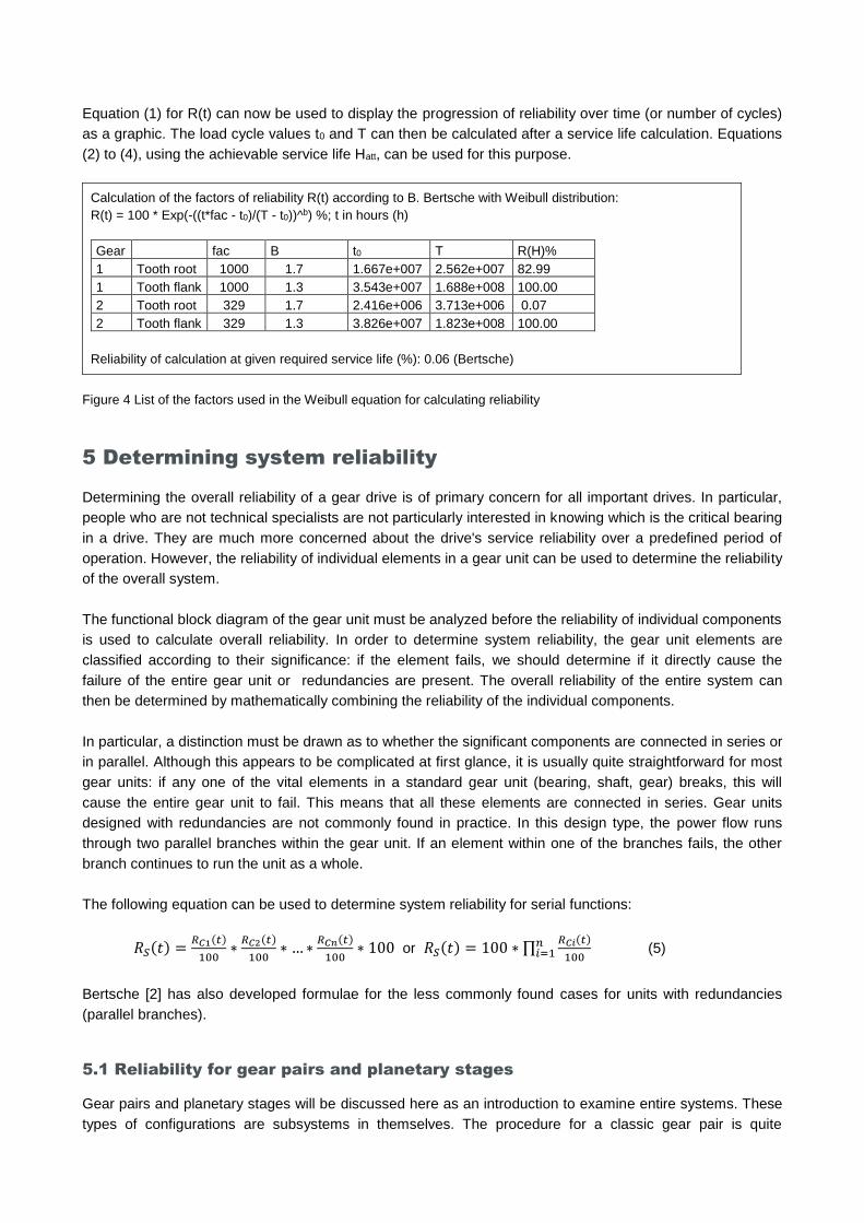
Equation (1) for R(t) can now be used to display the progression of reliability over time (or number of cycles)
as a graphic. The load cycle values t0 and T can then be calculated after a service life calculation. Equations
(2) to (4), using the achievable service life Hatt, can be used for this purpose.
Calculation of the factors of reliability R(t) according to B. Bertsche with Weibull distribution:
R(t) = 100 * Exp(-((t*fac - t0)/(T - t0))^b) %; t in hours (h)
Gear fac B t0 T R(H)%
1 Tooth root 1000 1.7 1.667e+007 2.562e+007 82.99
1 Tooth flank 1000 1.3 3.543e+007 1.688e+008 100.00
2 Tooth root 329 1.7 2.416e+006 3.713e+006 0.07
2 Tooth flank 329 1.3 3.826e+007 1.823e+008 100.00
Reliability of calculation at given required service life (%): 0.06 (Bertsche)
Figure 4 List of the factors used in the Weibull equation for calculating reliability
5 Determining system reliability
Determining the overall reliability of a gear drive is of primary concern for all important drives. In particular,
people who are not technical specialists are not particularly interested in knowing which is the critical bearing
in a drive. They are much more concerned about the drive's service reliability over a predefined period of
operation. However, the reliability of individual elements in a gear unit can be used to determine the reliability
of the overall system.
The functional block diagram of the gear unit must be analyzed before the reliability of individual components
is used to calculate overall reliability. In order to determine system reliability, the gear unit elements are
classified according to their significance: if the element fails, we should determine if it directly cause the
failure of the entire gear unit or redundancies are present. The overall reliability of the entire system can
then be determined by mathematically combining the reliability of the individual components.
In particular, a distinction must be drawn as to whether the significant components are connected in series or
in parallel. Although this appears to be complicated at first glance, it is usually quite straightforward for most
gear units: if any one of the vital elements in a standard gear unit (bearing, shaft, gear) breaks, this will
cause the entire gear unit to fail. This means that all these elements are connected in series. Gear units
designed with redundancies are not commonly found in practice. In this design type, the power flow runs
through two parallel branches within the gear unit. If an element within one of the branches fails, the other
branch continues to run the unit as a whole.
The following equation can be used to determine system reliability for serial functions:
𝑅𝑆(𝑡) =𝑅𝐶1(𝑡)
100∗
𝑅𝐶2(𝑡)
100∗ … ∗
𝑅𝐶𝑛(𝑡)
100∗ 100 or 𝑅𝑆(𝑡) = 100 ∗ ∏
𝑅𝐶𝑖(𝑡)
100𝑛𝑖=1 (5)
Bertsche [2] has also developed formulae for the less commonly found cases for units with redundancies
(parallel branches).
5.1 Reliability for gear pairs and planetary stages
Gear pairs and planetary stages will be discussed here as an introduction to examine entire systems. These
types of configurations are subsystems in themselves. The procedure for a classic gear pair is quite
straightforward: the overall reliability is the product of the four "elements" – tooth root (f) and tooth flank (h),
for the pinion (1) and the gear (2) in each case:
𝑅𝑝𝑎𝑖𝑟(𝑡) =𝑅𝑓1(𝑡)
100∗
𝑅ℎ1(𝑡)
100∗
𝑅𝑓2(𝑡)
100∗
𝑅ℎ2(𝑡)
100∗ 100 (6)
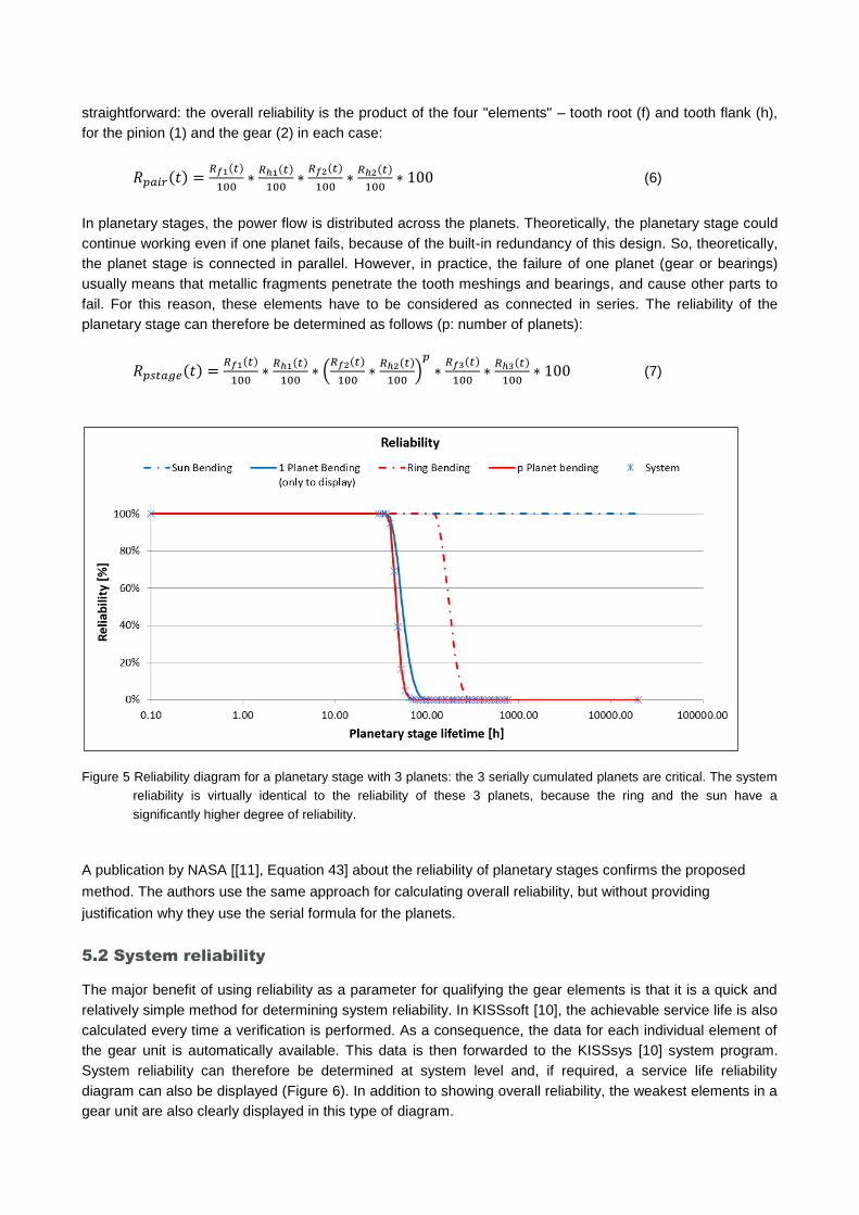
In planetary stages, the power flow is distributed across the planets. Theoretically, the planetary stage could
continue working even if one planet fails, because of the built-in redundancy of this design. So, theoretically,
the planet stage is connected in parallel. However, in practice, the failure of one planet (gear or bearings)
usually means that metallic fragments penetrate the tooth meshings and bearings, and cause other parts to
fail. For this reason, these elements have to be considered as connected in series. The reliability of the
planetary stage can therefore be determined as follows (p: number of planets):
𝑅𝑝𝑠𝑡𝑎𝑔𝑒(𝑡) =𝑅𝑓1(𝑡)
100∗
𝑅ℎ1(𝑡)
100∗ (
𝑅𝑓2(𝑡)
100∗
𝑅ℎ2(𝑡)
100)
𝑝
∗𝑅𝑓3(𝑡)
100∗
𝑅ℎ3(𝑡)
100∗ 100 (7)
Figure 5 Reliability diagram for a planetary stage with 3 planets: the 3 serially cumulated planets are critical. The system
reliability is virtually identical to the reliability of these 3 planets, because the ring and the sun have a
significantly higher degree of reliability.
A publication by NASA [[11], Equation 43] about the reliability of planetary stages confirms the proposed
method. The authors use the same approach for calculating overall reliability, but without providing
justification why they use the serial formula for the planets.
5.2 System reliability
The major benefit of using reliability as a parameter for qualifying the gear elements is that it is a quick and
relatively simple method for determining system reliability. In KISSsoft [10], the achievable service life is also
calculated every time a verification is performed. As a consequence, the data for each individual element of
the gear unit is automatically available. This data is then forwarded to the KISSsys [10] system program.
System reliability can therefore be determined at system level and, if required, a service life reliability
diagram can also be displayed (Figure 6). In addition to showing overall reliability, the weakest elements in a
gear unit are also clearly displayed in this type of diagram.
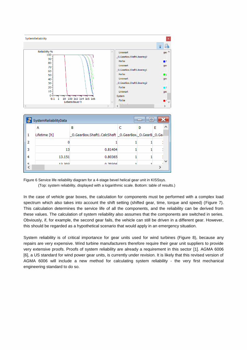
Figure 6 Service life reliability diagram for a 4-stage bevel helical gear unit in KISSsys.
(Top: system reliability, displayed with a logarithmic scale. Bottom: table of results.)
In the case of vehicle gear boxes, the calculation for components must be performed with a complex load
spectrum which also takes into account the shift setting (shifted gear, time, torque and speed) (Figure 7).
This calculation determines the service life of all the components, and the reliability can be derived from
these values. The calculation of system reliability also assumes that the components are switched in series.
Obviously, if, for example, the second gear fails, the vehicle can still be driven in a different gear. However,
this should be regarded as a hypothetical scenario that would apply in an emergency situation.
System reliability is of critical importance for gear units used for wind turbines (Figure 8), because any
repairs are very expensive. Wind turbine manufacturers therefore require their gear unit suppliers to provide
very extensive proofs. Proofs of system reliability are already a requirement in this sector [1]. AGMA 6006
[6], a US standard for wind power gear units, is currently under revision. It is likely that this revised version of
AGMA 6006 will include a new method for calculating system reliability - the very first mechanical
engineering standard to do so.
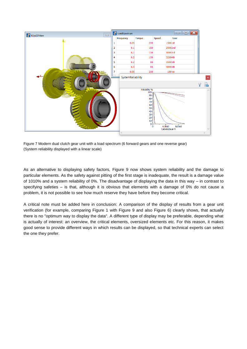
Figure 7 Modern dual clutch gear unit with a load spectrum (6 forward gears and one reverse gear)
(System reliability displayed with a linear scale)
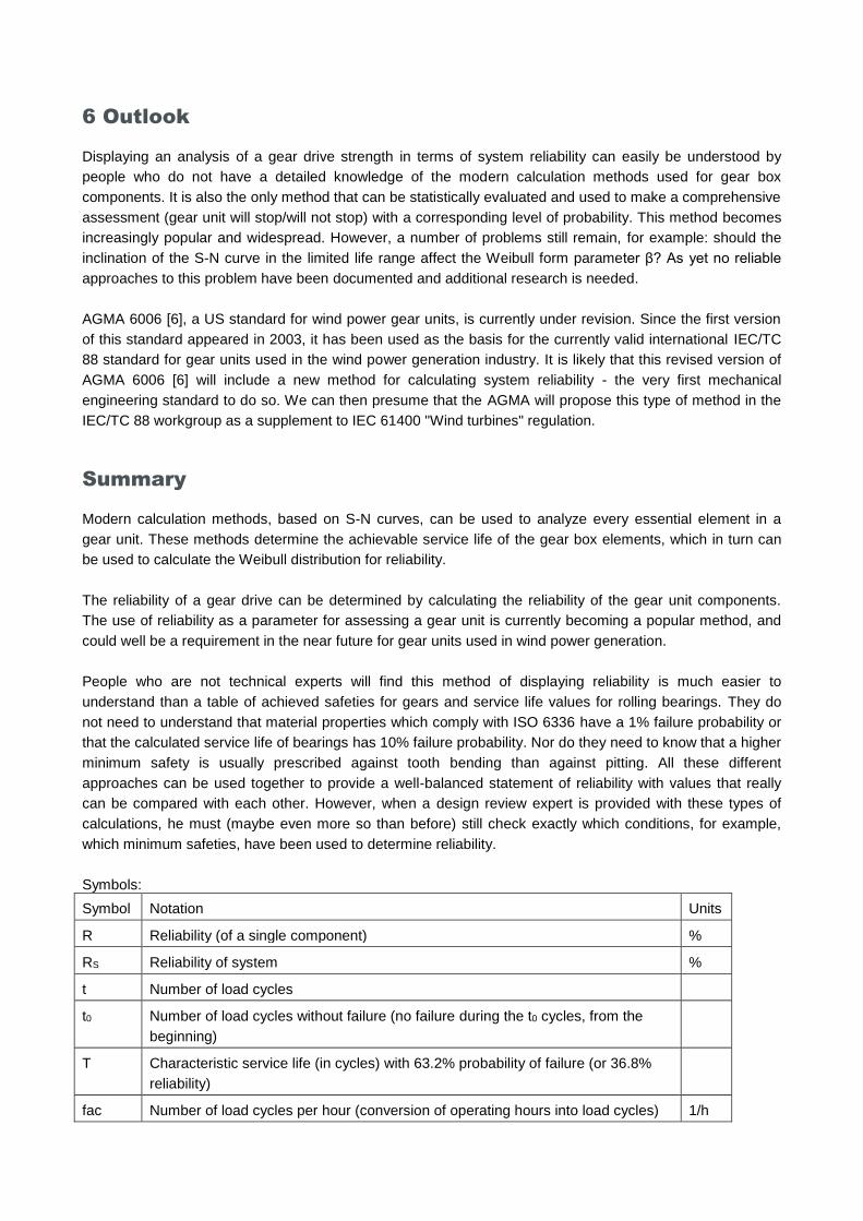
As an alternative to displaying safety factors, Figure 9 now shows system reliability and the damage to
particular elements. As the safety against pitting of the first stage is inadequate, the result is a damage value
of 1010% and a system reliability of 0%. The disadvantage of displaying the data in this way – in contrast to
specifying safeties – is that, although it is obvious that elements with a damage of 0% do not cause a
problem, it is not possible to see how much reserve they have before they become critical.
A critical note must be added here in conclusion: A comparison of the display of results from a gear unit
verification (for example, comparing Figure 1 with Figure 9 and also Figure 6) clearly shows, that actually
there is no "optimum way to display the data". A different type of display may be preferable, depending what
is actually of interest: an overview, the critical elements, oversized elements etc. For this reason, it makes
good sense to provide different ways in which results can be displayed, so that technical experts can select
the one they prefer.
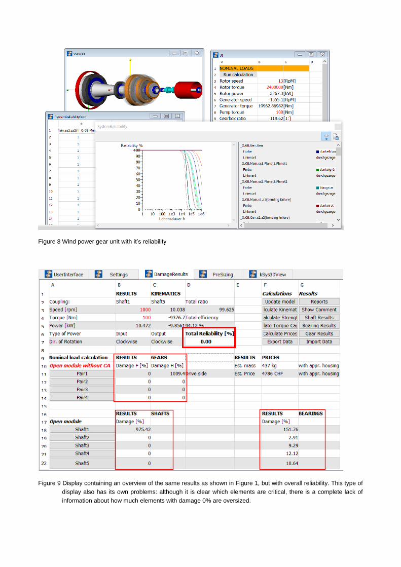
Figure 8 Wind power gear unit with it’s reliability
Figure 9 Display containing an overview of the same results as shown in Figure 1, but with overall reliability. This type of
display also has its own problems: although it is clear which elements are critical, there is a complete lack of
information about how much elements with damage 0% are oversized.
6 Outlook
Displaying an analysis of a gear drive strength in terms of system reliability can easily be understood by
people who do not have a detailed knowledge of the modern calculation methods used for gear box
components. It is also the only method that can be statistically evaluated and used to make a comprehensive
assessment (gear unit will stop/will not stop) with a corresponding level of probability. This method becomes
increasingly popular and widespread. However, a number of problems still remain, for example: should the
inclination of the S-N curve in the limited life range affect the Weibull form parameter β? As yet no reliable
approaches to this problem have been documented and additional research is needed.
AGMA 6006 [6], a US standard for wind power gear units, is currently under revision. Since the first version
of this standard appeared in 2003, it has been used as the basis for the currently valid international IEC/TC
88 standard for gear units used in the wind power generation industry. It is likely that this revised version of
AGMA 6006 [6] will include a new method for calculating system reliability - the very first mechanical
engineering standard to do so. We can then presume that the AGMA will propose this type of method in the
IEC/TC 88 workgroup as a supplement to IEC 61400 "Wind turbines" regulation.
Summary
Modern calculation methods, based on S-N curves, can be used to analyze every essential element in a
gear unit. These methods determine the achievable service life of the gear box elements, which in turn can
be used to calculate the Weibull distribution for reliability.
The reliability of a gear drive can be determined by calculating the reliability of the gear unit components.
The use of reliability as a parameter for assessing a gear unit is currently becoming a popular method, and
could well be a requirement in the near future for gear units used in wind power generation.
People who are not technical experts will find this method of displaying reliability is much easier to
understand than a table of achieved safeties for gears and service life values for rolling bearings. They do
not need to understand that material properties which comply with ISO 6336 have a 1% failure probability or
that the calculated service life of bearings has 10% failure probability. Nor do they need to know that a higher
minimum safety is usually prescribed against tooth bending than against pitting. All these different
approaches can be used together to provide a well-balanced statement of reliability with values that really
can be compared with each other. However, when a design review expert is provided with these types of
calculations, he must (maybe even more so than before) still check exactly which conditions, for example,
which minimum safeties, have been used to determine reliability.
Symbols:
Symbol Notation Units
R Reliability (of a single component) %
RS Reliability of system %
t Number of load cycles
t0 Number of load cycles without failure (no failure during the t0 cycles, from the
beginning)
T Characteristic service life (in cycles) with 63.2% probability of failure (or 36.8%
reliability)
fac Number of load cycles per hour (conversion of operating hours into load cycles) 1/h
Β Weibull form parameter
ftB Factor according to Table 2
Hatt Achievable service life of the component (in hours) h
Hatt10 Achievable service life of the component with 10% probability of failure h
Fo Specific probability of failure (for calculation of Hatt according to Table 1) %
Literature
[1] Falko, T.; Strasser, D et al.: Determination of the Reliability for a Multi-Megawatt Wind Energy Gearbox;
VDI report no.2255, 2015
[2] Bertsche, B.: Reliability in Automotive and Mechanical Engineering; Berlin, Heidelberg: Springer Verlag,
2008
[3] ISO 281, Rolling bearings — Dynamic load ratings and rating life, ISO, 2007
[4] ISO 6336, Part 1-6: Calculation of load capacity of spur and helical gears, ISO, 2006
[5] AGMA 6001-D97: Design and Selection of Components for Enclosed Gear Drives; AGMA, 1997
[6] AGMA 6006-B??: Revision of the Standard for Design and Specification of Gearboxes for Wind
Turbines; AGMA, 2003, Restricted document
[7] DIN 743, Tragfähigkeitsberechnung von Wellen und Achsen, 2012. (Calculation of load capacity of
shafts and axles)
[8] DIN 3990: Tragfähigkeitsberechnung von Stirnrädern; 1987 (Calculation of load capacity of cylindrical
gears)
[9] FKM Guideline, Rechnerischer Festigkeitsnachweis für Maschinenbauteile, 2012
[10] KISSsoft/KISSsys; Calculation Programs for Machine Design; www.KISSsoft.AG
[11] M.Savage, C.A.Paridon, Reliability Model for Planetary Gear Trains, NASA Technical Memorandum,
1982, http://www.dtic.mil/dtic/tr/fulltext/u2/a119165.pdf
[12] ISO/PDTS xxxxx-1: Calculation of tooth flank fracture load capacity of cylindrical spur and helical gears
– Part 1: Introduction and basic principles, ISO, 2015
[13] VDI 2230: Systematische Berechnung hochbeanspruchter Schraubenverbindungen (Systematic
calculation of highly stressed bolted joints), VDI, 2015
Recommended