Download pdf - Friction-stir welding of AA 2198 butt joints: mechanical characterization of the process and of the welds through DOE analysis

ORIGINAL ARTICLE

Friction-stir welding of AA 2198 butt joints: mechanicalcharacterization of the process and of the weldsthrough DOE analysis

Ciro Bitondo & Umberto Prisco & Antonino Squilace &

Pasquale Buonadonna & Gennaro Dionoro

Received: 9 June 2010 /Accepted: 28 July 2010 /Published online: 15 August 2010# Springer-Verlag London Limited 2010

Abstract In this study, rolled plates of AA 2198 T3aluminium alloy are friction-stir welded in butt config-uration varying two fundamental process parameters:rotational and welding speeds. Two sets of empiricalmodels based on regression analysis are developed. Thefirst one predicts the stationary values of the in-plane anddownwards forging welding forces in dependence of theprocess parameters under investigation. The second onepredicts the mechanical strength, in particular yield andtensile strength, of the friction-stir welded joints asfunction of the same parameters. For the developmentof the empirical models, two 32 full factorial designs areused: one having the stationary values of the weldingforces and the other having the yield and tensile strengthas observed responses, respectively. Statistical tools suchas analysis of variance, F tests, Mallows’ CP, coefficientof determination etc. are used to build and to validate thedeveloped models. By using the desirability functionapproach, the optimum process parameters to simulta-neously obtain maximum possible yield and tensilestrength are found within the investigated range. Thedeveloped models can be effectively used to predict thestationary forces and the mechanical proprieties of thejoints at 95% confidence level.

Keywords AA 2198 . Friction-stir welding (FSW) .

Rotational speed .Welding speed . FSW forces . Tensilestrength . Design of experiments, desirability function (DF)approach

1 Introduction

Friction-stir welding (FSW) is a solid-state joiningprocess in which the material that is being welded doesnot reach the melting point, in contrast to the fusionwelding processes [1]. Due to the interesting features ofFSW, lots of research activities have been carried out ondifferent materials (aluminium alloys first of all, but alsosteel, titanium, magnesium, copper, polymers etc.) and ondifferent weld geometries. In particular, FSW of AA 2198aluminium alloy has gained wide use in the fabrication oflightweight structures requiring a high strength-to-weightratio and good corrosion resistance [2].

In comparison with other welding techniques, FSWoffers advantages for low residual stresses, low distortionand high joint strength [2, 3]. Nevertheless, during thisprocess, the tool, with its rotational and welding speeds,exerts in-plane (horizontal) and downward (vertical)forging forces on the plates to be welded. These forces,joined to the thermal impact effect, may cause thedeformation of the fixture and of the welded plates, aswell as influence the tool wear. Hence, controlling theforce is mandatory for FSW and can have strongconsequences on the productivity and on the weld quality.Many significant benefits can be obtained keeping thewelding forces at a definite level: optimization of fixtur-ing, tool breakage prevention, tool life prediction, predic-tion of clamping forces, etc. Especially in robotic FSW,force controlling can be very helpful.

C. Bitondo :U. Prisco (*) :A. SquilaceDepartment of Materials and Production Engineering,University of Napoli Federico II,Piazzale Tecchio,Naples, Italye-mail: [email protected]

P. Buonadonna :G. DionoroDepartment of Mechanical Engineering, University of Cagliari,Piazza d’Armi,Cagliari, Italy

Int J Adv Manuf Technol (2011) 53:505–516DOI 10.1007/s00170-010-2879-9

However, to build an efficient control technique forFSW, a well-founded force prediction model needs to bedeveloped. The empirical model developed for the predic-tion of the welding forces can be further employed to getbetter insights into the mechanics of FSW, the correlationbetween the welding parameters and interdependencebetween the welding parameters and the weld quality.Development of FSW force models is not an easy taskconsidering that it was proved that the clamping forcecontains static nonlinearities with respect to the toolrotational speed, longitudinal speed, tool plunge depth andthe thermomechanical performance of the materials [3]. Onthe other side, it is also essential to have a complete controlover the relevant process parameters to maximize the yieldand tensile strength on which the quality of a weldment isbased.

It has been proved by several researchers that efficientuse of statistical design of experimental techniques allowsdevelopment of an empirical methodology to incorporate ascientific approach in the FSW procedure [4–8]. Indeed, thedesign of experiments was used in several papers toconduct experimental campaigns for exploring the interde-pendence of process parameters, and to develop empiricalmodels for the prediction of tensile strength of friction-stirwelded joints.

For instance, using the design of experiments concept,response surface method and the Hooke and Jeevesalgorithm, Elangovan et al. [6] developed a empiricalmodel to predict the tensile strength of friction-stir weldedAA 6061 aluminium alloy joints and optimized the FSWprocess parameters to attain maximum tensile strength. Themodel was developed by incorporating welding parametersand tool profiles and by using statistical tools such asdesign of experiments and regression analysis. Balasubra-manian [7] established an empirical relationships to predictthe FSW process parameters, in particular, tool rotationalspeed and welding speed, to fabricate defect free jointsfrom the known base metal properties (yield strength,ductility and hardness) of aluminium alloys. Lakshminar-ayanan et al. [8], based on a three factors three-level centralcomposite design with full replications, developed aresponse surface methodology to predict the tensile strengthof friction-stir welded AA7039 aluminium alloy.

However, to the present authors' knowledge, sparsework has been carried out on prediction of both weldingforces and mechanical proprieties of joints in FSW.

Therefore, in this investigation an attempt is made todevelop empirical models for the prediction of weldingforces and mechanical strength (yield and tensile) offriction-stir welded joints. In addition, it is tried tooptimize the FSW process parameters to attain maximummechanical strength of friction-stir welded joints using thedesirability function approach.

2 Experimental work

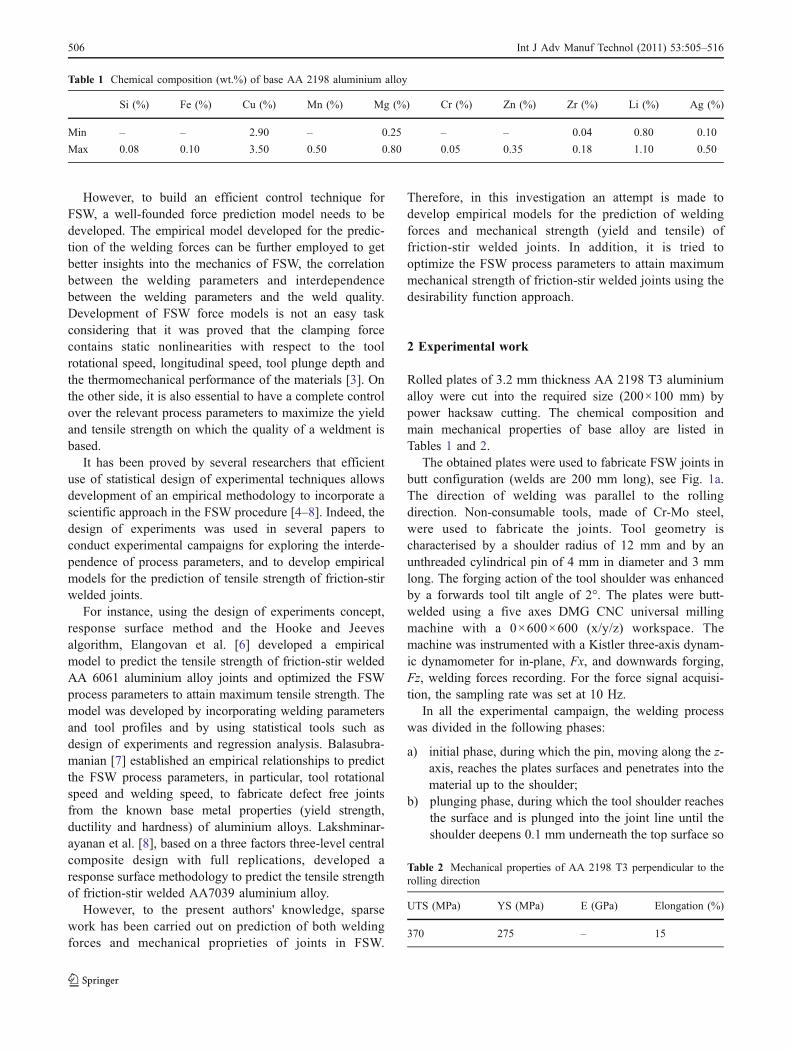
Rolled plates of 3.2 mm thickness AA 2198 T3 aluminiumalloy were cut into the required size (200×100 mm) bypower hacksaw cutting. The chemical composition andmain mechanical properties of base alloy are listed inTables 1 and 2.

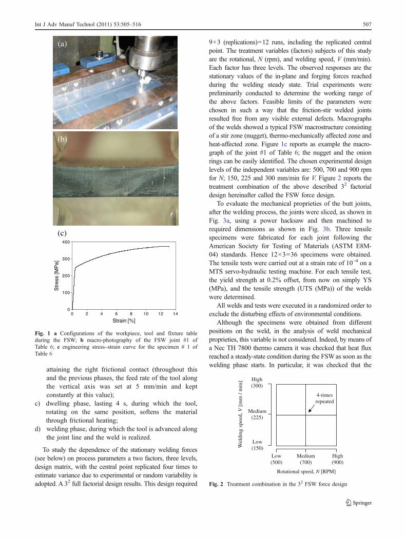
The obtained plates were used to fabricate FSW joints inbutt configuration (welds are 200 mm long), see Fig. 1a.The direction of welding was parallel to the rollingdirection. Non-consumable tools, made of Cr-Mo steel,were used to fabricate the joints. Tool geometry ischaracterised by a shoulder radius of 12 mm and by anunthreaded cylindrical pin of 4 mm in diameter and 3 mmlong. The forging action of the tool shoulder was enhancedby a forwards tool tilt angle of 2°. The plates were butt-welded using a five axes DMG CNC universal millingmachine with a 0×600×600 (x/y/z) workspace. Themachine was instrumented with a Kistler three-axis dynam-ic dynamometer for in-plane, Fx, and downwards forging,Fz, welding forces recording. For the force signal acquisi-tion, the sampling rate was set at 10 Hz.

In all the experimental campaign, the welding processwas divided in the following phases:

a) initial phase, during which the pin, moving along the z-axis, reaches the plates surfaces and penetrates into thematerial up to the shoulder;

b) plunging phase, during which the tool shoulder reachesthe surface and is plunged into the joint line until theshoulder deepens 0.1 mm underneath the top surface so

Table 1 Chemical composition (wt.%) of base AA 2198 aluminium alloy

Si (%) Fe (%) Cu (%) Mn (%) Mg (%) Cr (%) Zn (%) Zr (%) Li (%) Ag (%)

Min – – 2.90 – 0.25 – – 0.04 0.80 0.10

Max 0.08 0.10 3.50 0.50 0.80 0.05 0.35 0.18 1.10 0.50

Table 2 Mechanical properties of AA 2198 T3 perpendicular to therolling direction

UTS (MPa) YS (MPa) E (GPa) Elongation (%)

370 275 – 15

506 Int J Adv Manuf Technol (2011) 53:505–516

attaining the right frictional contact (throughout thisand the previous phases, the feed rate of the tool alongthe vertical axis was set at 5 mm/min and keptconstantly at this value);

c) dwelling phase, lasting 4 s, during which the tool,rotating on the same position, softens the materialthrough frictional heating;

d) welding phase, during which the tool is advanced alongthe joint line and the weld is realized.

To study the dependence of the stationary welding forces(see below) on process parameters a two factors, three levels,design matrix, with the central point replicated four times toestimate variance due to experimental or random variability isadopted. A 32 full factorial design results. This design required

9+3 (replications)=12 runs, including the replicated centralpoint. The treatment variables (factors) subjects of this studyare the rotational, N (rpm), and welding speed, V (mm/min).Each factor has three levels. The observed responses are thestationary values of the in-plane and forging forces reachedduring the welding steady state. Trial experiments werepreliminarily conducted to determine the working range ofthe above factors. Feasible limits of the parameters werechosen in such a way that the friction-stir welded jointsresulted free from any visible external defects. Macrographsof the welds showed a typical FSW macrostructure consistingof a stir zone (nugget), thermo-mechanically affected zone andheat-affected zone. Figure 1c reports as example the macro-graph of the joint #1 of Table 6; the nugget and the onionrings can be easily identified. The chosen experimental designlevels of the independent variables are: 500, 700 and 900 rpmfor N; 150, 225 and 300 mm/min for V. Figure 2 reports thetreatment combination of the above described 32 factorialdesign hereinafter called the FSW force design.

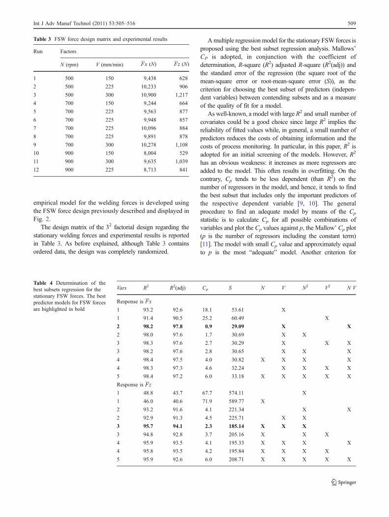
To evaluate the mechanical proprieties of the butt joints,after the welding process, the joints were sliced, as shown inFig. 3a, using a power hacksaw and then machined torequired dimensions as shown in Fig. 3b. Three tensilespecimens were fabricated for each joint following theAmerican Society for Testing of Materials (ASTM E8M-04) standards. Hence 12×3=36 specimens were obtained.The tensile tests were carried out at a strain rate of 10−4 on aMTS servo-hydraulic testing machine. For each tensile test,the yield strength at 0.2% offset, from now on simply YS(MPa), and the tensile strength (UTS (MPa)) of the weldswere determined.

All welds and tests were executed in a randomized order toexclude the disturbing effects of environmental conditions.

Although the specimens were obtained from differentpositions on the weld, in the analysis of weld mechanicalproprieties, this variable is not considered. Indeed, by means ofa Nec TH 7800 thermo camera it was checked that heat fluxreached a steady-state condition during the FSWas soon as thewelding phase starts. In particular, it was checked that the

Rotational speed, N [RPM]

Low (500)

Medium (700)

High(900)

Low(150)

Medium (225)

High (300)

Wel

ding

spe

ed, V

[m

m /

min

]

4-times repeated

Fig. 2 Treatment combination in the 32 FSW force design

(a)

(b)

Strain [%]0 2 4 6 8 10 12 14

Str

ess

[MP

a]

0

100

200

300

400

(c)

Fig. 1 a Configurations of the workpiece, tool and fixture tableduring the FSW; b macro-photography of the FSW joint #1 ofTable 6; c engineering stress–strain curve for the specimen # 1 ofTable 6

Int J Adv Manuf Technol (2011) 53:505–516 507

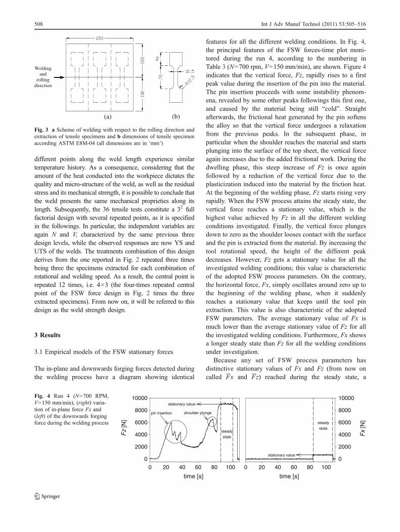
different points along the weld length experience similartemperature history. As a consequence, considering that theamount of the heat conducted into the workpiece dictates thequality and micro-structure of the weld, as well as the residualstress and its mechanical strength, it is possible to conclude thatthe weld presents the same mechanical proprieties along itslength. Subsequently, the 36 tensile tests constitute a 32 fullfactorial design with several repeated points, as it is specifiedin the followings. In particular, the independent variables areagain N and V, characterized by the same previous threedesign levels, while the observed responses are now YS andUTS of the welds. The treatments combination of this designderives from the one reported in Fig. 2 repeated three timesbeing three the specimens extracted for each combination ofrotational and welding speed. As a result, the central point isrepeated 12 times, i.e. 4×3 (the four-times repeated centralpoint of the FSW force design in Fig. 2 times the threeextracted specimens). From now on, it will be referred to thisdesign as the weld strength design.

3 Results

3.1 Empirical models of the FSW stationary forces

The in-plane and downwards forging forces detected duringthe welding process have a diagram showing identical

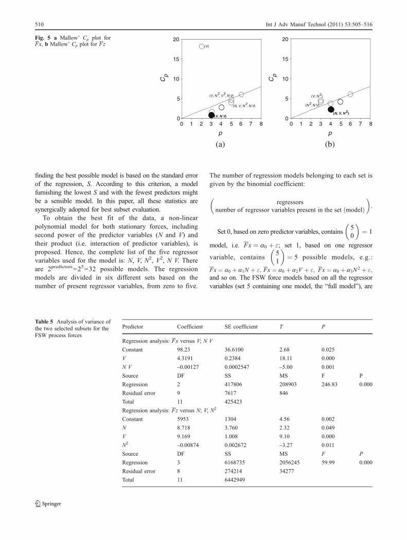
features for all the different welding conditions. In Fig. 4,the principal features of the FSW forces-time plot moni-tored during the run 4, according to the numbering inTable 3 (N=700 rpm, V=150 mm/min), are shown. Figure 4indicates that the vertical force, Fz, rapidly rises to a firstpeak value during the insertion of the pin into the material.The pin insertion proceeds with some instability phenom-ena, revealed by some other peaks followings this first one,and caused by the material being still “cold”. Straightafterwards, the frictional heat generated by the pin softensthe alloy so that the vertical force undergoes a relaxationfrom the previous peaks. In the subsequent phase, inparticular when the shoulder reaches the material and startsplunging into the surface of the top sheet, the vertical forceagain increases due to the added frictional work. During thedwelling phase, this steep increase of Fz is once againfollowed by a reduction of the vertical force due to theplasticization induced into the material by the friction heat.At the beginning of the welding phase, Fz starts rising veryrapidly. When the FSW process attains the steady state, thevertical force reaches a stationary value, which is thehighest value achieved by Fz in all the different weldingconditions investigated. Finally, the vertical force plungesdown to zero as the shoulder looses contact with the surfaceand the pin is extracted from the material. By increasing thetool rotational speed, the height of the different peakdecreases. However, Fz gets a stationary value for all theinvestigated welding conditions; this value is characteristicof the adopted FSW process parameters. On the contrary,the horizontal force, Fx, simply oscillates around zero up tothe beginning of the welding phase, when it suddenlyreaches a stationary value that keeps until the tool pinextraction. This value is also characteristic of the adoptedFSW parameters. The average stationary value of Fx ismuch lower than the average stationary value of Fz for allthe investigated welding conditions. Furthermore, Fx showsa longer steady state than Fz for all the welding conditionsunder investigation.

Because any set of FSW process parameters hasdistinctive stationary values of Fx and Fz (from now oncalled Fx and Fz) reached during the steady state, a

(a)

(b)

Weldingand

rollingdirection

Fig. 3 a Scheme of welding with respect to the rolling direction andextraction of tensile specimens and b dimensions of tensile specimenaccording ASTM E8M-04 (all dimensions are in ‘mm’)

time [s]

0 20 40 60 80 100

Fz

[N]

0

2000

4000

6000

8000

10000

time [s]

0 20 40 60 80 100

Fx

[N]

0

2000

4000

6000

8000

10000

steadystate

steadystate

stationary value

stationary value

pin insertion shoulder plunge

Fig. 4 Run 4 (N=700 RPM,V=150 mm/min), (right) varia-tion of in-plane force Fx and(left) of the downwards forgingforce during the welding process


empirical model for the welding forces is developed usingthe FSW force design previously described and displayed inFig. 2.

The design matrix of the 32 factorial design regarding thestationary welding forces and experimental results is reportedin Table 3. As before explained, although Table 3 containsordered data, the design was completely randomized.

Amultiple regressionmodel for the stationary FSW forces isproposed using the best subset regression analysis. Mallows’CP is adopted, in conjunction with the coefficient ofdetermination, R-square (R2) adjusted R-square (R2(adj)) andthe standard error of the regression (the square root of themean-square error or root-mean-square error (S)), as thecriterion for choosing the best subset of predictors (indepen-dent variables) between contending subsets and as a measureof the quality of fit for a model.

As well-known, a model with large R2 and small number ofcovariates could be a good choice since large R2 implies thereliability of fitted values while, in general, a small number ofpredictors reduces the costs of obtaining information and thecosts of process monitoring. In particular, in this paper, R2 isadopted for an initial screening of the models. However, R2

has an obvious weakness: it increases as more regressors areadded to the model. This often results in overfitting. On thecontrary, Cp tends to be less dependent (than R2) on thenumber of regressors in the model, and hence, it tends to findthe best subset that includes only the important predictors ofthe respective dependent variable [9, 10]. The generalprocedure to find an adequate model by means of the Cp

statistic is to calculate Cp for all possible combinations ofvariables and plot the Cp values against p, the Mallow’ Cp plot(p is the number of regressors including the constant term)[11]. The model with small Cp value and approximately equalto p is the most “adequate” model. Another criterion for

Table 3 FSW force design matrix and experimental results

Run Factors

N (rpm) V (mm/min) Fx (N) Fz (N)

1 500 150 9,438 628

2 500 225 10,233 906

3 500 300 10,900 1,217

4 700 150 9,244 664

5 700 225 9,563 877

6 700 225 9,948 857

7 700 225 10,096 884

8 700 225 9,891 878

9 700 300 10,278 1,108

10 900 150 8,004 529

11 900 300 9,635 1,039

12 900 225 8,713 841

Vars R2 R2(adj) Cp S N V N2 V2 N V

Response is Fx

1 93.2 92.6 18.1 53.61 X

1 91.4 90.5 25.2 60.49 X

2 98.2 97.8 0.9 29.09 X X

2 98.0 97.6 1.7 30.69 X X

3 98.3 97.6 2.7 30.29 X X X

3 98.2 97.6 2.8 30.65 X X X

4 98.4 97.5 4.0 30.82 X X X X

4 98.3 97.3 4.6 32.24 X X X X

5 98.4 97.2 6.0 33.18 X X X X X

Response is Fz

1 48.8 43.7 67.7 574.11 X

1 46.0 40.6 71.9 589.77 X

2 93.2 91.6 4.1 221.34 X X

2 92.9 91.3 4.5 225.71 X X

3 95.7 94.1 2.3 185.14 X X X

3 94.8 92.8 3.7 205.16 X X X

4 95.9 93.5 4.1 195.33 X X X X

4 95.8 93.5 4.2 195.84 X X X X

5 95.9 92.6 6.0 208.71 X X X X X

Table 4 Determination of thebest subsets regression for thestationary FSW forces. The bestpredictor models for FSW forcesare highlighted in bold


finding the best possible model is based on the standard errorof the regression, S. According to this criterion, a modelfurnishing the lowest S and with the fewest predictors mightbe a sensible model. In this paper, all these statistics aresynergically adopted for best subset evaluation.

To obtain the best fit of the data, a non-linearpolynomial model for both stationary forces, includingsecond power of the predictor variables (N and V) andtheir product (i.e. interaction of predictor variables), isproposed. Hence, the complete list of the five regressorvariables used for the model is: N, V, N2, V2, N V. Thereare 2predictors=25=32 possible models. The regressionmodels are divided in six different sets based on thenumber of present regressor variables, from zero to five.

The number of regression models belonging to each set isgiven by the binomial coefficient:

regressorsnumber of regressor variables present in the set modelð Þ

� �:

Set 0, based on zero predictor variables, contains50

� �¼ 1

model, i.e. Fx ¼ a0 þ "; set 1, based on one regressor

variable, contains51

� �¼ 5 possible models, e.g.:

Fx ¼ a0 þ a1N þ "; Fx ¼ a0 þ a2V þ "; Fx ¼ a0 þ a3N2 þ ";

and so on. The FSW force models based on all the regressorvariables (set 5 containing one model, the “full model”), are

p

Cp

0

5

10

15

20

(V, N2, V

2, N V)

(N, V, N2, N V)

(V, N V)

(V)

(a)

p

0 1 2 3 4 5 6 7 80 1 2 3 4 5 6 7 8

Cp

0

5

10

15

20

(V, N 2)

(N, V, N 2)

(N 2, N V)

(b)

Fig. 5 a Mallow’ Cp plot forFx, b Mallow’ Cp plot for Fz

Predictor Coefficient SE coefficient T P

Regression analysis: Fx versus V; N V

Constant 98.23 36.6100 2.68 0.025

V 4.3191 0.2384 18.11 0.000

N V –0.00127 0.0002547 –5.00 0.001

Source DF SS MS F P

Regression 2 417806 208903 246.83 0.000

Residual error 9 7617 846

Total 11 425423

Regression analysis: Fz versus N; V; N2

Constant 5953 1304 4.56 0.002

N 8.718 3.760 2.32 0.049

V 9.169 1.008 9.10 0.000

N2 –0.00874 0.002672 –3.27 0.011

Source DF SS MS F P

Regression 3 6168735 2056245 59.99 0.000

Residual error 8 274214 34277

Total 11 6442949

Table 5 Analysis of variance ofthe two selected subsets for theFSW process forces


written as:

Fx ¼ a0 þ a1N þ a2V þ a3N2 þ a4V

2 þ a5N � V þ "

and

Fz ¼ b0 þ b1N þ b2V þ b3N2 þ b4V

2 þ b5N � V þ ":

In Table 4 the values of the statistics used in theprocedure of best subset selection are reported. For everyset, one or two models with larger R2 are shown. In the

above-mentioned table, Vars is the numbers of variables inthe model; R2 and R2(adj) are converted to percentages;predictors that are present in the model are indicated by anX. In Fig. 5, for each model and for each stationary forcevalue, the analysis is completed plotting Cp against p, withthe line Cp=p added.

Those which are assessed as best predictor models forFSW forces are highlighted in bold in Fig. 5 and in Table 4;in particular, for Fx the best subset seems the onecontaining V and N V as predictor variables and for Fz itis the one with the predictor variables N, V and N2. They areboth minimum-Cp subsets showing the maximum R2(adj)and an acceptable small number of variable amid theregressions under inspection. The fitness of the models isfurther confirmed by a satisfactory value of determinationcoefficient, R2, which is calculated to be 0.982 and 0.957for Fx and Fz, respectively, indicating that 98.2% and 95.7of the variability in the response could be predicted by themodels. It is not worth increasing the variable numberbecause this does not cause a significant gain in R2 (for Fxthe full model shows an R2 of 0.984 and for Fz an R2 of0.959). Furthermore, their (p, Cp) value is enough close tothe line X = Y.

The models adequacy is confirmed by the F testsreported in Table 5: the analysis of variance shows thatthe selected regression models are highly significant.Indeed, it is calculated P<0.001 with an F value of246.83 [F0.001(2,9)=16.38] and P<0.001 with an F valueof 59.99 [F0.001(3,8)=15.82] for the Fx and Fz regressions,respectively. All the coefficients are evaluated and testedfor their significance at 95% confidence level, applying thestudent's t test. The regression coefficients, along with thecorresponding P values, are shown in the same Table 5.

Then, the final empirical model developed to predict Fxis given below as:

Fx ¼ 98:23þ 4:32 V � 0:00127 N � V ;while the force along z-axis is regressed as:

Fz ¼ 5; 953þ 8:72 N þ 9:17 V � 0:00874 N 2:

Conformity of the presented models to the assumptionsunderlying regression analysis (normally and independentlydistributed errors with mean zero, homoscedasticity of theerrors etc.) were checked using classical statistical tools asresidual plots, normal probability plots of the residuals etc.Results of these analyses are not reported for the sake ofshortness.

It is very interesting to note that both stationary FSWforces depend on the regressor variable V and, in particular,they become larger increasing the welding velocity, as it isexpected. Besides V, Fx presents only the interaction termbetween N and V; this term is present with the minus signpreceding it and a very small coefficient, conferring an

Table 6 Weld strength design matrix and experimental results

Run Factors

N (rpm) V (mm/min) YS (MPa) UTS (MPa)

1 500 150 248 370

2 500 150 246 368

3 500 150 246 338

4 500 225 252 375

5 500 225 249 289

6 500 225 250 364

7 500 300 252 339

8 500 300 253 360

9 500 300 255 370

10 700 150 247 354

11 700 150 244 355

12 700 150 244 345

13 700 225 254 326

14 700 225 252 343

15 700 225 254 341

16 700 225 252 321

17 700 225 253 302

18 700 225 252 320

19 700 225 254 305

20 700 225 252 306

21 700 225 254 321

22 700 225 254 305

23 700 225 252 263

24 700 225 251 309

25 700 300 252 310

26 700 300 252 312

27 700 300 251 318

28 900 150 246 294

29 900 150 239 295

30 900 150 247 314

31 900 225 245 290

32 900 225 247 260

33 900 225 244 261

34 900 300 248 286

35 900 300 259 292

36 900 300 252 290


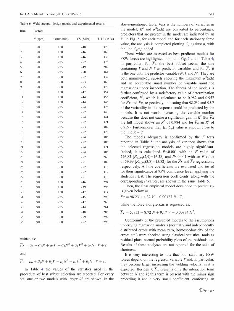
extremely slight curvature to the function, which looks likea simple series of almost parallel lines that generally occurwith first order models, see the counter plot in Fig. 6a.However, the final effect is that the in-plane force decreasesas N rises and grows increasing V. Apart the positivedependence on V, the downwards forging force, Fz,decreases as the rotational speed becomes larger, seeFig. 6b, and this effect is more manifest than for Fx, dueto the quite evident curvature conferred to the function bythe presence of the N2 term; this curvature is especially

evident at high values of V and low values of N. However,as it has been already experimentally observed [3, 4, 12],the welding speed has little effect on the FSW forces, whileincreasing the rotational speed causes a significant decreaseof their stationary values. Obviously, this is determined bythe greater heat production resulting from the higherrotational speed. In conclusion, Fx and Fz are characterizedby a simple and analogous dependence upon N and V:basically, they strongly decrease increasing N, and slightlyincrease with V.

V [

mm

/ m

in]

1000

900

800

700

60 0

1100

500 600 700 800 900 500 600 700 800 900150

180

210

240

270

300

V [

mm

/ m

in]

9000

8500

9500

10000

10500

150

180

210

240

270

300

N [RPM] N [RPM]

(b)(a)

Fig. 6 a Contour plot of Fx, bcontour plot of Fz

Table 7 Determination of the best subsets regression for YS and UTS. The best predictor models for YS and UTS are highlighted in bold

Vars R2 R2(adj) Cp S N V N2 V2 N V

Response is YS

1 42.7 41.0 13.5 3.13 X

1 38.0 36.2 17.2 3.26 X

2 52.9 50.1 7.4 2.88 X X

2 50.3 47.3 9.4 2.96 X X

3 58.5 54.6 4.9 2.75 X X X

3 58.3 54.3 5.1 2.75 X X X

4 61.5 56.5 4.6 2.69 X X X X

4 59.1 53.8 6.5 2.77 X X X X

5 62.2 55.9 6.0 2.71 X X X X X

Response is UTS

1 53.6 52.2 8.7 22.23 X

1 53.1 51.7 9.1 22.35 X

2 58.7 56.2 6.1 21.28 X X

2 57.5 54.9 7.2 21.59 X X

3 65.5 62.3 2.2 19.75 X X X

3 64.6 61.3 3.0 20.00 X X X

4 65.6 61.2 4.1 20.04 X X X X

4 65.6 61.1 4.2 20.05 X X X X

5 65.8 60.0 6.0 20.33 X X X X X


3.2 Empirical models of the mechanical strengthof the welds

The weld strength design matrix and experimental results ofthe 36 tensile tests are reported in Table 6. Figure 1c reportsas example the engineering stress–strain curve for thespecimen #1 of Table 6.

A second order polynomial model is proposed for YSand UTS as function of N and V. Again, YS and UTSregression analyses are tested against the followingregression variables: N, V, N2, V2, N V. The best subsetof terms to be included in the model is defined usingMallows’ CP in conjunction with R2, R2(adj) and S.Table 7 contains the results obtained for the determinationof the best subsets regression. As done before, for eachnumber of terms included in the model under investigation

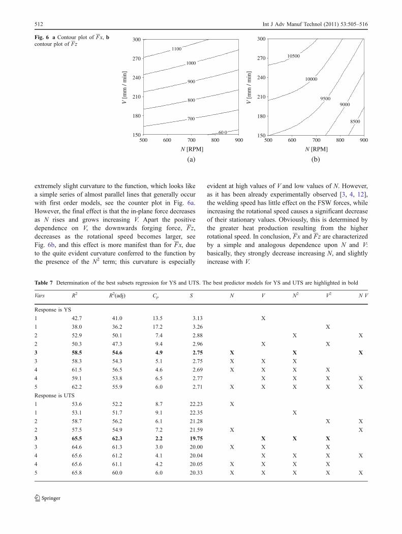
the two models individuated by larger R2 are displayed.Figure 7a, b reports the Mallow’ Cp plots for YS and UTS.The models assessed as best are highlighted (in bold) inTable 7 and Fig. 7.

For YS, (N, N2, N V) is selected as best regressionsubset. Although, the (N, V, N2, V2) subset shows a lowerCp, it is rejected due to its larger number of regressionvariables. Indeed, it is worthless to adopt a more compli-cated four-variable model when, swapping the three-variable model for the four-variable one, a little profit isrealized in terms of S; specifically, S passes from 2.75 to2.69. Moreover, the chosen model has a good Cp and afairly excellent R-Sq(adj), compared to the other models.

From the elaboration of UTS data, the regression modelcontaining the terms V, N2, V2 is picked out. Maximizingthe adjusted determination coefficients and minimizing S,

p

Cp

0

5

10

15

20

(V )

(V 2)

(N 2, N V )

(N, N 2, N V ) (N, V, N 2, V 2)

(V, N 2, V 2, N V )

(V, V 2)

(a)

p0 1 2 3 4 5 6 7 80 1 2 3 4 5 6 7 8

Cp

0

5

10

15

20

(V, N2, V

2)

(N, N V )

(V 2, N V )

(N 2)

(b)

Fig. 7 a Mallow’ Cp plot forYS, (b) Mallow’ Cp plot forUTS

Predictor Coef SE Coef T P

Regression analysis: YS versus N, N2, N V

Constant 224.69 11.02 20.38 0.000

V 0.0672 0.03238 2.08 0.046

N2 −0.00006389 0.00002293 −2.79 0.009

N V 0.00006925 0.00001203 5.76 0.000

Source DF SS MS F P

Regression 3 341.63 113.88 15.04 0.000

Residual error 32 242.26 7.57

Total 35 583.89

Regression analysis: UTS versus V, N2, V2

Constant 564.89 58.71 9.62 0.000

V −1.6131 0.5308 −3.04 0.005

N2 −0.00011768 0.00001656 −7.11 0.000

V2 0.003328 0.001172 2.84 0.008

Source DF SS MS F P

Regression 3 23,721.0 7,907.0 20.25 0.000

Residual Error 32 12,493.2 390.4

Total 35 36,214.1

Table 8 Analysis of variance ofthe two selected subsets for themechanical proprieties of thewelds


this combination is distinctly recognized as the best subset.Moreover, the model contains a fairly low number of terms,so avoiding redundant information.

The analyses of variance of the models adopted for YSand UTS, in Table 8, confirm the correctness of the subsets.The analyses show that these regression models are highlysignificant: P<0.001 with F value of 15.04 and P<0.001with F value of 20.25 for YS and UTS regressions,respectively [F0.001(3, 32)=6.93]. All the evaluated coef-ficients pass the t test used to check their significance at95% confidence level. The regression coefficients, alongwith the corresponding P values, are shown in the sameTable 8.

Then, the final empirical models developed to predictYS and UTS are:

YS ¼ 224:69þ 0:0672 � N � 0:000064 � N2 þ 0:000069 � N � V ;UTS ¼ 564:89� 1:6131 � V � 0:00011768 � N 2 þ 0:003328 � V 2:

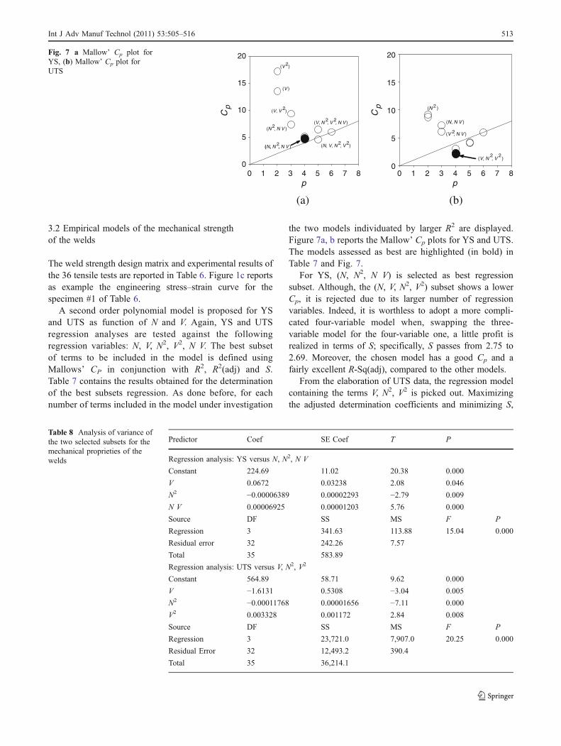
YS depends on N and N2. The interaction term between Nand V is also present as the elliptical contours clearly indicate[13], see Fig. 8a. It is possible to conclude, by examining thecontour plot in Fig. 8a, that YS is a little more sensitive tochanges in welding speed than to changes in rotational speed.UTS is a function of V and V2; furthermore, it also depends onN2. Indeed, Fig. 8b exhibits almost circular contours, surely

more circular than YS, which suggest a larger independenceof factor effects, namely N and V. Finally, UTS seems moresensitive to changes in N than to changes in V, as it is evidentfrom Fig. 8b.

The contour plots shown in Fig. 8 clearly bring out amore complex behaviour of YS and UTS, compared to thewelding forces, which simply increase with V and decreasewith N. In particular, the optimum YS is exhibited forvalues of N at the middle of the working range, around680/700 rpm, and for high values of V, about 300 mm/min,while, the optimum UTS is obtained at medium values ofV, nearly 240 mm/min, and high values of N, around900 rpm.

3.3 Optimising FSW parameters to maximise YS and UTS

To maximize the weld mechanical strength, i.e. tooptimize both YS and UTS, on which the quality of aweldment is based, it is essential to select and control the

V [

mm

/ m

in]

252

250

248

246

244

254

500 600 700 800 900 500 600 700 800 900150

180

210

240

270

300

V [

mm

/ m

in]

280

280

300

300

320

320

340

340

360150

180

210

240

270

300

N [RPM] N [RPM]

(a) (b)

Fig. 8 a Contour plot of YS, bcontour plot of UTS

Table 9 Result of the multiresponse optimization

Optimum value=0.8404

Factor Response Low High Optimum

N 500 900 531

V 150 300 300

UTS 348

YS 253

V [

mm

/ m

in]

0, 3

0, 1

0, 2

0,2

0, 4

0,3

0, 3

0,5

0, 4

0, 4

0, 5

0, 6

0, 5

0, 6

0,7

0, 6

0,7

0, 8

500 600 700 800 900150

180

210

240

270

300

N [RPM]

Fig. 9 Contour plot of the overall desirability function for the levelsof rotational and welding speeds


welding process parameters, N and V. However, theprevious analysis showed that the welding processparameters for which it is possible to achieve themaximum UTS do not match with those maximizing theYS. A typical multiresponse optimization problem, in-volving conflicting responses, arises. In this paper, asimultaneous optimization technique, based on the desir-ability function (DF) [14, 15] is used to optimize themultiple responses, YS and UTS. In particular, the DFapproach is used to find the best compromise between thetwo responses, based on the empirical equations aboveestablished for YS and UTS.

The DF approach transforms an estimated response (e.g.,the ith estimated response byi) into a scale-free value, calleddesirability function, denoted as di for byi, di byið Þ. It is a valuebetween 0 and 1, increasing as the corresponding responsevalue becomes more desirable. If the response is to bemaximized, as in this case, the individual desirability isgenerally defined as

di byið Þ ¼0 if byi < Libyi�LiUi�Li

if Li � byi � Ui

1 if byi > Ui

8<: :;

where Li and Ui are the lower and upper values, respectively,for response byi. The overall desirability D, another valuebetween 0 and 1, is defined by the weighted geometric meanof the individual desirability values (i.e., di’s):

D ¼ dw11 � dw2

2 � dw33 :::::; 0 < wi < 1 andw1 þ w2 þ w3 þ :::

¼ 1;

where wi is the relative importance assigned to the responsei. The relative importance is a comparative scale forweighting each of the resulting di in the overall desirabilityproduct. It is noteworthy that the outcome of the overalldesirability D depends on the wi value, which offers usersflexibility in the definition of desirability functions. Theoptimal setting is determined by maximizing D, beingevident that D will increase when the balance of theproperties becomes more favourable.

In this study, the responses, YS and UTS, are trans-formed into appropriate desirability scales d1 and d2according to the following equations:

d1 ¼0 if YS < YS minYS�YS min

YS max�YS minif YS min � YS � YS max

1 if YS > YS max

8<: ;

d2 ¼0 if UTS < UTS minUTS�UTS min

UTS max�UTS minif UTS min � UTS � UTS max

1 if UTS > UTS max

8<: ;

where YSmax, YSmin and UTSmax, UTSmin are calculated bymeans of the preceding regression equations.

Clearly, d1 and d2 increase as long as YS and UTSincrease. The overall desirability D was calculated by

D ¼ d1 � d2;

because the same importance is attributed to the differentresponses, namely w1=w2=1.

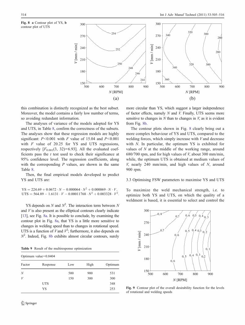
The results of the optimization are reported in Table 9,where the maximum global desirability function (D=0.8404), the best achievable of each of the responses, YSand UTS, and the optimal welding parameters, N and V, arepresented. In addition, the optimization results are alsoillustrated with the contour plots of D, in Fig. 9.

The optimal result is obtained at N=531 rpm and V=300 mm/min, which correspond to UTS=348 MPa andYS=253 MPa. At this operating condition, the empiricalmodels previously developed for the FSW forces predictthat the stationary welding forces are: Fx ¼ 1;191N andFz ¼ 15;798N.

4 Conclusion

& Two sets of empirical models, containing rotational andwelding speeds as independent variables, are developedat 95% confidence level. The first one predicts the in-plane and downward forging forces in the FSW of AA2198 butt joints. The second one predicts the yield andtensile strengths of the friction stir welded AA 2198butt joints. The models are developed using statisticaltools such as design of experiments and regressionanalysis. The choice of the predictive variables to beincluded in the model is carried out by means of theMallows’ Cp. in conjunction with R2, R2(adj) and thestandard error of the regression.

& Contour plots are drawn to study the interaction effectof the welding parameters under study on FSW forcesand mechanical strength of friction stir welded joints ofthe AA 2198 aluminium alloy. Welding forces demon-strate a simple and analogous dependence upon processparameters under concern: they decrease increasing therotational speed and slightly rise with the weldingspeed, however following dissimilar laws. On thecontrary, yield and tensile strengths show a verydifferent dependence on rotational and welding speeds.In particular, they reach their maximum for differentand incompatible values of the process parameter understudy.

& The desirability function approach is used forsimultaneous optimization of yield and tensilestrengths of the friction stir welded AA 2198 buttjoints. The multi-objective optimization methodsindicates that best quality joints can be manufacturedby using the optimal conditions of 531 rpm and


300 mm/min for rotational and welding speed,respectively, namely realizing the FSW in the so-called cold condition.

& The method developed in this work may provide anattractive solution to simultaneous optimization ofseveral response variables, allowing high performanceproduction. The results are expected to be helpful inoptimizing the FSW process and in facilitating itsautomation to ensure good weld quality.

References

1. Thomas WM (1991) Friction stir welding, international patentapplication no. PCT/GB92/02203 and GB Patent Application No.9125978.8, December, US Patent No. 5,460,317

2. Cavaliere P, De Santis A, Panella F, Squillace A (2009) A effect ofanisotropy on fatigue properties of 2198 Al–Li plates joined byfriction stir welding. Eng Fail Anal 16:1856–1865

3. Chen C, Kovacevic R (2004) Thermomechanical modelling andforce analysis of friction stir welding by the finite elementmethod. J Mech Eng Sci C 218:509–519

4. Prisco A, Acerra F, Squillace A, Giorleo G, Pirozzi C, Prisco U,Bellucci F (2008) LBW of similar and dissimilar skin-stringerjoints. Part I: process optimization and mechanical characteriza-tion. Adv Mater Res 38:306–319

5. Elangovan K, Balasubramanian V, Babu S (2009) Predictingtensile strength of friction stir welded AA6061 aluminium alloyjoints by a empirical model. Mater Des 30:188–193

6. Elangovan K, Balasubramanian V, Babu S, Balasubramanian M(2008) Optimising friction stir welding parameters to maximisetensile strength of AA6061 aluminium alloy joints. Int J ManufRes 3:321–334

7. Balasubramanian V (2008) Relationship between base metalproperties and friction stir welding process parameters. MaterSci Eng A 480:397–403

8. Lakshminarayanan AK, Balasubramanian V (2009) Comparisonof RSM with ANN in predicting tensile strength of friction stirwelded AA7039 aluminium alloy joints. Trans Nonferr Met SocChina 19:9–18

9. Hocking RR, Leslie RN (1967) Selection of the best subset inregression analysis. Technometrics 9:531–540

10. Mallows CL (1973) Some comments on Cp. Technometrics15:661–675

11. Mallows CL (1995) More comments on Cp. Technometrics37:362–372

12. Balasubramanian N, Gattu B, Mishra RS (2009) Process forcesduring friction stir welding of aluminium alloys. Sci Technol WeldJoin 14:141–145

13. Montgomery DC (2001) Design and analysis of experiments.Wiley, New York

14. Harrington E Jr (1965) The desirability function. Industr QualControl 21:494–498

15. Derringer G, Suich R (1980) Simultaneous optimization of severalresponse variables. J Qual Technol 12:214–219
