FORECASTS OF SUPPLY – DEMAND OF FOODGRAINS AND OTHER FOOD ITEMS
OVER THE MEDIUM TERM FUTURE
PARMOD KUMAR
Prof & Head, ADRTC,
Institute for Social and Economic Change
Bangalore - 560072

Estimating Demand & Supply Systems
A Methodological Note
ISEC Nagarbhavi PO
Bangalore
India
April 9, 2015 NCAER New Delhi

Outline
Estimation of Demand Model
complete demand system - all consumable items
The Model : Almost Ideal Demand System
Properties of Demand System
Data Base – Consumption and Prices
Assumption on Demand Projections
Estimation of Supply Model
OLS Estimates of Area, Yield, Prices and
Exports
Simultaneous Equation Model – 3
SLS
Data Base
Assumptions for supply Projections

Basic properties of a demand model
Adding-up: Budget shares sum to one, i.e., total expenditure must be exhausted among individual commodities
Homogeneity condition: Demand functions are homogenous of degree zero in prices and income.
Symmetry condition: Slutsky’s symmetry condition implies that the compensated cross price elasticities are equal.
Negativity condition: Compensated demand curve is downward sloping or the substitution effect is always negative implying that the ‘law of demand’ holds.

The Almost Ideal
Demand System (AIDS)
The AIDS model developed by Deaton and Muellbauer (1980) derive demand system by use of duality concepts, from a particular cost or expenditure function. The AIDS cost function is given by
Where α0 ,αi , βi and γij, are parameters, u is utility and pj’s are prices. AIDS
model satisfies the axioms of choice exactly, and does not impose additive preferences and under certain conditions, allows consistent aggregation of individual demands to market demands. By applying Shepard’s Lemma, that is, by differentiating the cost function, after appropriate substitutions, we obtain the AIDS in budget share form:

The Model
• Where P is price index defined by
• With the above price index, the system becomes non-linear and
requires estimation of a large number of parameters that needs a
long data series on budget shares, total expenditure and prices.
Deaton and Muellbauer (1980a) used Stone Price Index to make
the system linear by substituting ln P* = Σ wk ln pk ;
• where P ~= P*;

Parameter Restrictions
Adding up
Homogeneity Σyij = 0;
Symmetry Yij = Yji
The fourth restriction (concavity of the expenditure function) has no parametric representation.

Demographic representation
Following Heien and Pompelli (1988), demographic effects
are incorporated in the model by allowing the intercept to be
a function of demographic variables as:
Where dj is the jth demographic variable, the examples could
be household size, region, gender, education level of
household head, etc.

Two Stage Budgeting A two-stage
budgeting demand system: It
is supposed that the consumer
allocates her total budget in two
stages.
In the first stage, the consumer determines the
allocation of her total expenditure between various commodity groupings, e.g., cereals, pulses, edible oils,
milk-meat, fruit-vegetables, other food items and non-
food items.
In the second stage, the expenditure is allocated
among different groups, e.g., wheat, rice and coarse grains
among the cereal group; fruit, vegetables and nuts
among fruit-vegetables group and so on.
LA/AIDS model used to estimate the two stage-
budgeting demand function

Elasticity Formulation
Income elasticity:
own-price and cross-price elasticities
Where is Kronecker’s delta which is equal to unity for every s=r, and zero otherwise,

Data Base – Consumption All-India average monthly per capita consumer expenditure on food and
non food commodities and the corresponding per capita total consumer expenditure (PCE), separately for rural and urban households.
Unit level data of the National Sample Survey Organization (NSSO) for its 43rd to 66th rounds for ‘Household Consumption Expenditure’.
The time period consists of a continuous time series beginning from 1987-88 (43rd round) up to 2009-10 (66th round)
Model estimated at the aggregate and three population groups based on ranking by the level of PCE, viz., the poorest one fourth (bottom 25 percent), the middle half (middle 50 percent) and the upper one fourth (top 25 percent), separately for the rural and urban sector.

Data Base – Prices (Contd) The wholesale price indices published by the OEA. The price indices for the seven broad
groups of items as well as for the individual items are prepared at the base year 2004-05.
The price indices of all individual items for the whole time period (1987-88 to 2009-10) are first converted into 2004-05 prices (2004-05=100) through splicing. The individual items in the converted monthly price indices are matched with the items within each of the seven broad groups of the consumer expenditure to prepare wholesale price relatives in each group.
The monthly wholesale price relatives in each group are then averaged over the months covered by a NSS round to obtain the average price relative for that round in each group.
Using the expenditure weights for individual items in a broad group relative to the total expenditure on the broad group, separately for rural and urban areas, the price index relative for individual and broad group items are constructed for both rural and urban sectors.
The expenditure weights are worked out on the basis of estimated average consumer expenditure on individual items in each group, separately for rural and urban areas using the NSS 62nd (2004-05) round consumer expenditure per capita data.

Model Estimation
The LA/AIDS model
Non-linear seemingly unrelated regression method
Without and with imposing restriction of homogeneity, adding-up and symmetry.
The commodity combinations are:
Cereals - wheat, rice and coarse cereals;
Pulses
Edible oils
Milk - meat - milk and meat;
Fruits and vegetables - fruits, vegetables and dry-nuts;
Other food – sugar, spices, beverages and intoxicants
Non food

Assumptions for Demand Projections
India’s decadal population growth rate - 1.97% PA (1991), 1.49% PA (2001), expected growth 1.17% PA in 2011.
Contribution of rural sector in total GDP (Net National Income) expected to come down from 48% in 1999-00 to 40% in 2008-09 and to 28 % in 2020-21.
NNP growth up to 2020– Three scenarios (i) 8.9 % (ii) 12% and (iii) 6% per annum
Corresponding PCI growth would be (i) 5.5-6% (ii) 8.5-9% and (iii) 2.7-3.2%.

Demand Projections – Formula
Where Qijt is household demand for ith commodity for the jth sub group
(rural or urban) during the tth time period; qij0 is the annual per capita quantity consumed of ith commodity by the jth sub group during the base year (2004-05); Pjt is the projected population of jth sub group in the year t; gjt is annual growth rate in per capita income for the jth sub group during the tth time period; and eij is the expenditure elasticity of the ith commodity for the jth sub group.

Estimation of Supply System:Simultaneous Model
Supply response function
Area function
Yield function
Price response function
Export function

Model Specification Area = f (Pi, Pj, Rain, Irrg, Fert, Fertp, Trend, Lagged)
Production = f (Pi, Rain, Irrg, Fert, Fertp, Trend, Lagged)
Real dom price = f (MSP, WP, Prod, WI, PD, Trend, Lagged)
Exports = f (Pi, WP, Prod, Open, PD, WT, WI, REER, Trend, Lagged)
Where
Pi is real domestic (farm harvest) price;
Pj is real competing crop price;
Rain is rainfall - annual, monsoon or winter months as applicable in different cases;
Irrg is percentage of area under irrigation
Fert is fertilizer use in kgs per hectare;
Fertp is real fertilizer price;
MSP is real minimum support price;
WP is real world price or real unit value of exports;
WI is real world income;
PD is policy dummy;
Open is openness in terms of share of Indian exports in the world exports commodity wise;
WT is volume of world trade in a particular commodity.
REER is real effective exchange rate

Specification of Crops (group of crops)
The specific crops are:
rice, wheat, kharif and rabi coarse cereals, kharif and rabi pulses and kharif and rabi oilseeds.
Crop sub-groups are:
Kharif Coarse Cereals: Jowar, Bajra, Ragi and Maize;
Rabi Coarse Cereals: Barley;
Kharif Pulses: Tur, Moong, Urad;
Rabi Pulses: Gram and Masoor (Lentil);
Kharif Oilseeds: Groundnut, Soyabeans, Sunflower, Sesamum, Nigerseed;
Rabi Oilseeds: Rapeseed & Mustard, Safflower and Linseed.

Expenditure elasticity Rural Urban
Rice -0.25 -0.002
Wheat -0.29 -0.001
C. cereals -0.96 -0.005
Cereals -0.33 -0.002
Pulses 0.55 0.017
Edible oils 0.90 0.35
Milk 0.86 0.45
Meat 1.25 0.43
Vegetables 1.02 0.21
Fruits 1.90 0.62
Nuts 0.95 0.63
Sugar 0.13 0.11
Spices 1.29 0.30
Beverages 1.04 0.26
Intoxicants 1.41 0.38
Non food 1.82 1.80

Household Demand Projections Using Expenditure Elasticities Rice Wheat Other
cereals
Total
cereals
Pulses Foodgrain
s
Edible oil Oilseeds
Actual demand
2009-10 80.23 61.43 9.97 151.63 9.78 161.41 9.76 34.9
Baseline (growth rate of NNP at 8.9 percent per annum)
2010-11 80.72 61.80 9.70 152.17 10.13 162.30 10.32 36.9
2012-13 81.38 62.33 9.15 152.65 10.83 163.49 11.49 41.0
2013-14 81.73 62.63 8.94 153.02 11.16 164.18 12.05 43.1
2014-15 82.02 62.89 8.70 153.23 11.52 164.75 12.69 45.3
2017-18 83.00 63.76 8.05 154.15 12.66 166.81 14.81 52.9
2020-21 84.17 64.83 7.52 155.50 13.93 169.42 17.28 61.7
High growth (growth rate of NNP at 12 percent per annum)
2010-11 80.27 61.42 9.46 151.05 10.24 161.29 10.53 37.6
2012-13 80.04 61.21 8.49 149.38 11.19 160.57 12.22 43.6
2013-14 79.96 61.16 8.11 148.74 11.65 160.39 13.07 46.7
2017-18 79.59 60.96 6.73 146.07 13.82 159.90 17.43 62.2
2020-21 79.62 61.11 5.98 144.88 15.73 160.60 21.62 77.2
Low growth (growth rate of NNP at 6 percent per annum)
2010-11 81.15 62.16 9.93 153.21 10.03 163.24 10.12 36.1
2012-13 82.65 63.40 9.80 155.77 10.51 166.28 10.84 38.7
2013-14 83.42 64.05 9.78 157.14 10.72 167.86 11.16 39.9
2017-18 86.35 66.55 9.57 162.23 11.69 173.92 12.71 45.4
2020-21 88.75 68.62 9.44 166.45 12.48 178.92 14.03 50.1

Indirect Demand for Seed, Feed, Wastage, Industrial and Other Indirect Uses (SFW) (million tonnes)
Rice Wheat C Cereals Pulses Foodgrains
1990–1995 5.5 10.7 13.0 4.7 34.0
1996–2000 7.6 15.5 17.7 4.2 45.0
2001–2006 4.2 16.3 18.7 3.7 42.8
2007–08 4.4 14.9 20.1 4.2 43.5
2008–09 4.4 15.6 21.0 4.1 45.2
2009–10 4.5 16.4 21.9 4.1 46.8
2010–11 4.6 17.1 22.8 4.0 48.6
2011–12 4.7 18.0 23.8 4.0 50.5
2012–13 4.7 18.8 24.9 4.0 52.4
2013–14 4.8 19.7 26.0 3.9 54.4
2014–15 4.9 20.6 27.1 3.9 56.5
2015–16 5.0 21.6 28.3 3.8 58.7
2016–17 5.1 22.6 29.6 3.8 61.0
2017–18 5.2 23.6 30.9 3.7 63.4
2018–19 5.2 24.8 32.2 3.7 65.9
2019–20 5.3 25.9 33.6 3.7 68.6
2020–21 5.4 27.1 35.1 3.6 71.3

Aggregate Demand (direct + indirect) Rice Wheat Other cer Total cer Pulses Foodgrains Edible oil Oilseeds
Actual demand
2009-10 84.74 77.80 31.85 194.39 13.87 208.25 9.76 34.9
Baseline (growth rate of NNP at 8.9 percent per annum)
2010-11 85.31 78.95 32.54 196.79 14.18 210.97 10.32 36.9
2012-13 86.12 81.13 34.04 201.29 14.79 216.08 11.49 41.0
2013-14 86.55 82.31 34.93 203.79 15.07 218.86 12.05 43.1
2015-16 87.31 84.73 36.79 208.83 15.72 224.55 13.36 47.7
2017-18 88.16 87.41 38.92 214.49 16.41 230.90 14.81 52.9
2020-21 89.60 91.97 42.64 224.21 17.55 241.76 17.28 61.7
High growth (growth rate of NNP at 12 percent per annum)
2010-11 84.85 78.56 32.29 195.71 14.28 209.99 10.53 37.6
2011-12 84.91 79.33 32.81 197.05 14.72 211.77 11.36 40.6
2012-13 84.77 80.00 33.39 198.16 15.15 213.31 12.22 43.6
2013-14 84.78 80.84 34.10 199.72 15.56 215.28 13.07 46.7
2015-16 84.71 82.57 35.69 202.97 16.52 219.48 15.09 53.9
2017-18 84.75 84.60 37.60 206.96 17.57 224.53 17.43 62.2
2020-21 85.04 88.25 41.11 214.41 19.35 233.75 21.62 77.2
Low growth (growth rate of NNP at 6 percent per annum)
2010-11 85.73 79.31 32.77 197.81 14.07 211.88 10.12 36.1
2011-12 86.67 80.80 33.72 201.20 14.28 215.48 10.49 37.5
2012-13 87.39 82.20 34.70 204.29 14.47 218.75 10.84 38.7
2015-16 89.83 86.84 37.99 214.67 15.02 229.69 11.91 42.5
2017-18 91.51 90.20 40.44 222.15 15.43 237.58 12.71 45.4
2020-21 94.18 95.76 44.56 234.50 16.10 250.60 14.03 50.1

Aggregate supply projections Period – I
2011 2012 2013 2014 2015 2016 2017 2018 2019 2020
Rice Area 44.0 42.2 44.3 44.4 44.5 44.4 44.4 44.3 44.2 44.1
Production 105.3 105.2 112.3 113.8 116.8 119.8 122.7 125.7 128.6 131.6
Export 7.2 10.1 6.7 6.8 7.0 7.1 7.2 7.3 7.5 7.6
Wheat Area 29.9 29.7 29.5 29.5 29.6 29.7 29.7 29.6 29.4 29.3
Production 94.9 93.5 95.5 97.2 99.6 103.3 103.8 103.6 103.3 103.0
Export 0.7 6.5 0.1 0.1 0.2 0.2 0.3 0.4 0.5 0.7
Other
Cereals
Area 26.4 24.6 25.4 25.2 24.8 24.2 23.4 22.7 21.8 21.0
Production 42.0 40.0 43.5 43.9 44.8 45.0 45.1 45.0 44.7 44.4
Export 4.0 5.2 5.7 5.3 4.9 4.5 4.1 3.7 3.3 3.0
Pulses Area 24.5 23.4 23.2 22.7 22.2 21.9 21.6 21.4 21.1 20.9
Production 17.1 18.3 16.4 15.9 15.8 15.6 15.6 15.5 15.5 15.5
Export 0.0 0.0 0.0 0.0 0.0 0.0 0.0 0.0 0.0 0.0
Total
Foodgrai
ns
Area 124.8 119.8 122.5 121.8 121.1 120.2 119.1 117.9 116.6 115.3
Production 259.3 257.1 267.7 270.9 277.0 283.7 287.1 289.8 292.2 294.5
Export 11.9 21.7 12.5 12.3 12.1 11.8 11.6 11.4 11.3 11.3
Oilseeds Area 26.3 26.5 29.6 30.3 31.0 31.7 32.5 33.3 34.4 35.4
Production 29.8 30.9 37.2 37.4 39.1 40.8 42.7 44.7 48.3 50.2
Export 1.3 1.0 1.3 1.2 1.2 1.1 1.0 1.0 0.9 0.9

Aggregate supply projections for foodgrains and oilseeds – All India
Period – II
2011 2012 2013 2014 2015 2016 2017 2018 2019 2020
Rice Area 44.0 42.2 45.0 45.5 45.9 46.3 46.6 46.9 47.2 47.5
Production 105.3 105.2 111.4 112.8 115.6 118.3 121.1 123.9 126.6 129.4
Export 7.2 10.1 7.7 8.4 9.1 9.7 10.4 11.0 11.7 12.3
Wheat Area 29.9 29.7 29.8 29.9 30.0 30.1 30.2 30.4 30.5 30.6
Production 94.9 93.5 93.6 94.6 96.0 97.4 98.9 100.3 101.8 103.4
Export 0.7 6.5 0.1 0.1 0.1 0.1 0.1 0.1 0.1 0.1
Other
Cereals
Area 26.4 24.6 26.6 27.2 27.7 28.1 28.4 28.6 28.8 28.9
Production 42.0 40.0 44.0 45.7 47.9 49.8 51.6 53.3 55.0 56.6
Export 4.0 5.2 6.3 6.6 7.3 8.2 9.4 10.9 12.8 15.1
Pulses Area 24.5 23.4 23.1 22.7 22.3 22.1 21.9 21.7 21.6 21.5
Production 17.1 18.3 16.4 15.9 15.8 15.7 15.7 15.7 15.7 15.8
Export 0.0 0.0 0.0 0.0 0.0 0.0 0.0 0.0 0.0 0.0
Total
Foodgrai
ns
Area 124.8 119.8 124.6 125.2 125.9 126.5 127.1 127.6 128.1 128.5
Production 259.3 257.1 265.4 269.1 275.3 281.3 287.3 293.2 299.2 305.2
Export 11.9 21.7 14.1 15.2 16.5 18.0 19.8 22.0 24.5 27.5
Oilseeds Area 26.3 26.5 29.3 29.8 30.3 30.7 31.1 31.6 32.0 32.4
Production 29.8 30.9 36.6 36.5 38.0 39.5 41.0 42.6 44.3 46.0
Export 1.3 1.0 1.7 1.9 2.0 2.2 2.4 2.6 2.8 3.0

Net balances of supply and demand of foodgrains and Oilseeds Rice Wheat Other
cereals
Total
cereals
Pulses Foodgrains Oilseeds
Without adjusting for exports
2011-12 Low 20.4 15.6 9.2 45.2 2.8 48.0 -7.7
2011-12 High 18.6 14.1 8.3 41.0 2.4 43.4 -10.8
2012-13 Low 20.5 13.5 6.7 40.6 3.9 44.5 -7.8
2012-13 High 17.9 11.3 5.3 34.5 3.2 37.7 -12.7
2013-14 Low 26.6 12.8 9.4 48.8 1.8 51.1 -3.3
2013-14 High 24.1 11.8 8.3 44.1 0.8 44.4 -9.5
2014-15 Low 28.0 13.0 9.1 50.1 1.1 53.0 -4.7
2014-15 High 24.8 12.0 8.9 45.7 -0.1 43.7 -12.8
2015-16 Low 30.9 13.4 9.1 53.3 0.8 57.3 -4.5
2015-16 High 27.0 12.8 9.9 49.7 -0.8 45.8 -14.8
2016-17 Low 33.6 13.9 8.4 55.9 0.4 61.2 -4.4
2016-17 High 29.1 14.8 10.6 54.5 -1.3 48.4 -17.1
2017-18 Low 36.3 14.3 7.5 58.1 0.1 64.7 -4.4
2017-18 High 31.2 13.6 11.2 55.9 -1.9 47.5 -19.5
2018-19 Low 39.0 14.6 6.3 59.9 -0.1 64.9 -4.3
2018-19 High 33.3 11.6 11.6 56.5 -2.4 49.0 -22.2
2019-20 Low 41.7 14.9 4.9 61.5 -0.4 71.6 -4.2
2019-20 High 35.3 9.5 11.9 56.7 -3.0 43.2 -23.6
2020-21 Low 44.4 14.8 3.3 62.5 -0.6 64.0 -4.1
2020-21 High 37.4 7.6 12.1 57.1 -3.6 51.3 -27.0

Net balances of supply and demand of foodgrains and Oilseeds Rice Wheat Other
cereals
Total
cereals
Pulses Foodgrains Oilseeds
After adjusting for exports
2011-12 Low 13.2 14.8 5.2 33.2 2.8 36.0 -9.0
2011-12 High 11.5 13.3 4.3 29.1 2.4 31.4 -12.1
2012-13 Low 10.3 7.0 1.5 18.9 3.9 22.8 -8.7
2012-13 High 7.7 4.8 0.2 12.8 3.2 15.9 -13.6
2013-14 Low 19.9 12.7 3.7 36.3 1.8 38.6 -4.6
2013-14 High 16.4 11.7 1.9 30.0 0.8 30.3 -11.3
2014-15 Low 21.2 12.8 3.8 37.8 1.1 40.7 -5.9
2014-15 High 16.4 11.9 2.2 30.5 -0.1 28.6 -14.7
2015-16 Low 23.9 13.2 4.2 41.3 0.8 45.2 -5.7
2015-16 High 17.9 12.7 2.7 33.3 -0.8 29.3 -16.9
2016-17 Low 26.5 13.6 4.0 44.1 0.4 49.4 -5.5
2016-17 High 19.4 14.7 2.5 36.5 -1.3 30.4 -19.3
2017-18 Low 29.1 14.0 3.4 46.5 0.1 53.1 -5.4
2017-18 High 20.9 13.5 1.8 36.1 -1.9 27.7 -21.9
2018-19 Low 31.7 14.2 2.6 48.5 -0.1 53.4 -5.2
2018-19 High 22.3 11.5 0.7 34.5 -2.4 27.0 -24.8
2019-20 Low 34.3 14.3 1.6 50.2 -0.4 60.3 -5.1
2019-20 High 23.7 9.4 -0.9 32.2 -3.0 18.7 -26.5
2020-21 Low 36.8 14.1 0.3 51.2 -0.6 52.7 -4.9
2020-21 High 25.1 7.5 -3.0 29.6 -3.6 23.8 -30.1
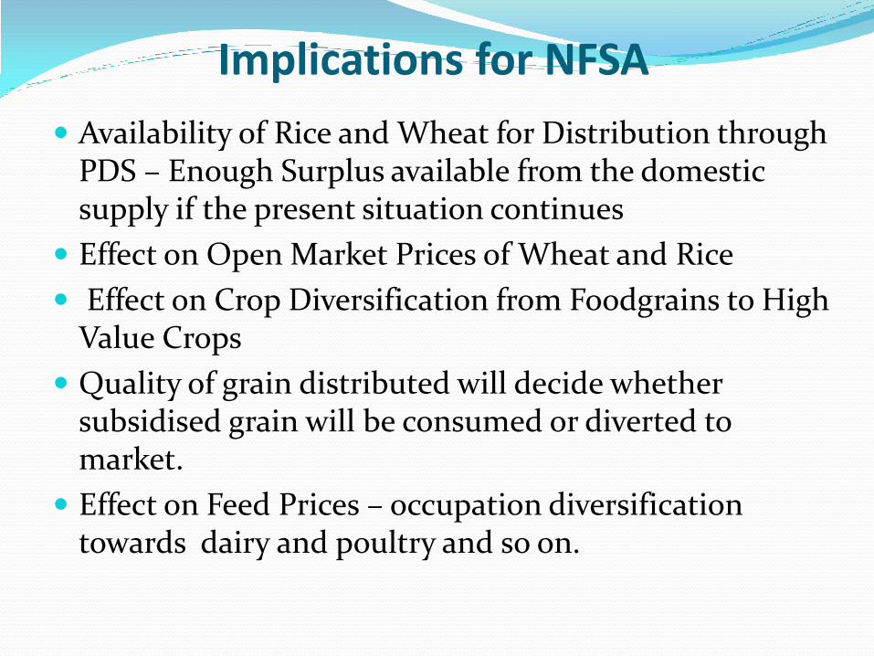
Implications for NFSA
Availability of Rice and Wheat for Distribution through PDS – Enough Surplus available from the domestic supply if the present situation continues
Effect on Open Market Prices of Wheat and Rice
Effect on Crop Diversification from Foodgrains to High Value Crops
Quality of grain distributed will decide whether subsidised grain will be consumed or diverted to market.
Effect on Feed Prices – occupation diversification towards dairy and poultry and so on.

Storage capacity and gap The peak demand for storage occurs on January and with Food Security Act,
grain procurement would go up. The Rangarajan Committee estimated a food distribution requirement ranging from 64 to 74 million tonnes of grain (Economic Advisory Council, 2011). With a 60-40 split between rice and wheat, the peak storage demand does not exceed 41 million tonnes even in the high requirement scenario of 74 million tonnes. To this figure, one can add the emergency/ strategic reserves of 5 million tonnes. The total peak storage would therefore be around 46 million tonnes.
Gap between required and existing storage capacity
The Food Corporation of India (FCI) - the central government agency responsible for procurement and storage of grain for the Public Distribution System (PDS) - has a storage capacity of 32 million tonnes, of which about half is hired. Hence, assuming that the FCI has hired all the capacity that is possible then the gap between FCI’s existing capacity (32 million tonnes) and the required capacity (46 million tonnes) is about 14 million tonnes. Incidentally, in the 11th Five Year Plan, the FCI identified a gap of 16 million tonnes of capacity that needed to be created.
There would be requirement of additional capacity of storage.
28

29
Subsidy Incurred by Food Corporation of India
(2009-2010 and 2011-2012)
(Rs. in Crore)
Particular 2009-10 2010-11 2011-12 (RE)
Acquisition Cost
Wheat 20417 26332 32888
Rice 32440 39279 56881
Coarsegrains 47 11 -
Sub Total 52904 65622 89769
Sales Realisation (CIP)
Wheat 9762 11380 12428
Rice 13126 13661 17943
Coarsegrains 14 4 -
Sub Total 22902 25045 30371
Subsidy On Acquisition Cost (Difference)
Operating Cost
Freight 3961 4289 4855
Handling 1873 2382 3213
Storage 1661 2175 2822
Interest 2403 1566 2904
Shortages 281 474 762
Admin Overheads 1027 1354 1562
Sub Total 9973 12240 16118
Interest on Clear Outstanding Food
Subsidy 895 1255 1829
Interest on Outstanding from RD/HRD 338 341 343
Total Operating Cost 11206 13836 18290
Carry-Over Charges Paid 1665 1981 2565
Total Gross Subsidy 42873 56394 80253
Food Subsidy Rs
80 thousand
crore when less
than 30%
population was
covered and
price for BPL
was much higher
compared to
AAY. How with
coverage of 67%
population with
cereal prices at
AAY scheme
would subsidy be
restricted to Rs
125 thousand
crore. Also the
lifting for AAY
was much higher
compared to
BPL so lifting
would be high in
FSB. Subsidy
unsustainable.

Thank You
Recommended