FNCE 30001 Investments 12.0
FNCE 30001 InvestmentsSemester 2, 2011
26 & 28 October 2009Week 12: Portfolio Performance
EvaluationProfessor Rob Brown

FNCE 30001 Investments 12.1
Lecture 11: Portfolio Performance Evaluation
Overview of Lecture1. Steps in performance evaluation2. Performance measurement3. Performance appraisal4. Performance attribution
Reading: Bodie et al, Chapter 24.“Performance Measurement” (pdf available on the LMS).

FNCE 30001 Investments 12.2
1. Steps in Performance Evaluation

FNCE 30001 Investments 12.3
Steps in Performance Evaluation1. Performance measurement
– Calculating the return that a portfolio achieved over a period of time.
2. Performance appraisal– Evaluating the overall performance of a portfolio.
3. Performance attribution– Determining what portion of this overall performance was
due to the manager’s skill in selecting securities.
Steps in Performance Evaluation

FNCE 30001 Investments 12.4
2. Performance Measurement

FNCE 30001 Investments 12.5
• Measuring past returns may be harder than you think.• Some issues are:
– Cash flows (eg quarterly) may not match the desired frequency of return measurement (eg annual).
– There may be multiple cash inflows and /or outflows due to (eg):• dividends• distributions to fund members• new funds invested• funds withdrawn• management fees
Performance Measurement

FNCE 30001 Investments 12.6
– Choice of measurement methodology:• “Time-weighted”
– geometric (discrete time) or – logarithmic (continuous time)
• “Dollar-weighted”– aka “internal rate of return”
Performance Measurement

FNCE 30001 Investments 12.7
• Over short periods of time there is often little difference between the methods.
• Over long periods of time, there may be larger differences.• We will tackle all these complications using examples.• We will start with the simplest case and work up to more
complex cases.
Performance Measurement

FNCE 30001 Investments 12.8
Example 1: One stock held for one period; no dividend.
Purchase price (P0) is $35.50.Sale price (P1) is $38.34. Sale occurs 6 months after purchase.What is the rate of return per half-year (discrete time)?
Performance Measurement
1 0
0Rate of return per half-year
$38.34 $35.50$35.50
$2.84$35.508.00% per half-year
P PP

FNCE 30001 Investments 12.9
Example 2: One stock held for one period; no dividend.
Same as Example 1, except we require an annual rate of return.The annual rate of return (discrete time) is given by:
– This is just the familiar idea of the effective interest rate applied in a slightly different context.
2R ate o f return pa 1 .0800 116 .64% pa
Performance Measurement

FNCE 30001 Investments 12.10
Example 2 (contd.)
More formally, in discrete time we assume that:
Performance Measurement
1 01
1
0
1 0.5
1 , which implies:
1
Here, is 6 months (half a year); so is 0.5.
$38.34 1$35.50
16.64% pa
n
n
P P r
PrP
n n
r

FNCE 30001 Investments 12.11
Example 3: One stock held for one period; no dividend.
Same as Example 2, except in continuous time.In continuous time, we assume that:
Performance Measurement
1 0
1
0
, which implies:
1 n
Here, is 6 months (half a year); so is 0.5. Hence,
1 $38.34n0.5 $35.502 0.07696104115.392% pa
r nP P e
Prn P
n n
r

FNCE 30001 Investments 12.12
Example 4: One stock held for one period; with dividend
Purchase price (P0) is $35.50; Sale price (P1) is $38.34 (ex-div).A dividend of 71 cents is paid after 6 months.What is the rate of return (discrete time) per year?
Performance Measurement
1 0 1
0
2
Rate of return per half-year
$3.55$35.5010.00% per half-year
Rate of return pa 1.1000 121.00% pa
P P DP

FNCE 30001 Investments 12.13
Example 5: One stock held for many periods; no dividends
Purchase 200 shares at $10.20 each and hold for 8 quarters.Outlay = 200 x $10.20 = $2040. Prices move as shown below.
Performance Measurement
Quarter (end) Price per share Portfolio value
0 $10.20 $2040
1 $9.80 $1960
2 $10.96 $2192
3 $11.25 $2250
4 $11.61 $2322
5 $11.75 $2350
6 $11.05 $2210
7 $11.85 $2370
8 $14.58 $2916

FNCE 30001 Investments 12.14
Example 5 (contd.)
Calculate:(a) Arithmetic and logarithmic rates of return for each quarter.(b) The total rate of return over the 8 quarters.(c) The mean rate of return per quarter and per annum.
Performance Measurement
1
1
1
Arithmetic RoR in quarter
Logarithmic RoR in quarter n
t t
t
t
t
P PtP
PtP
FNCE 30001 Investments 12.15
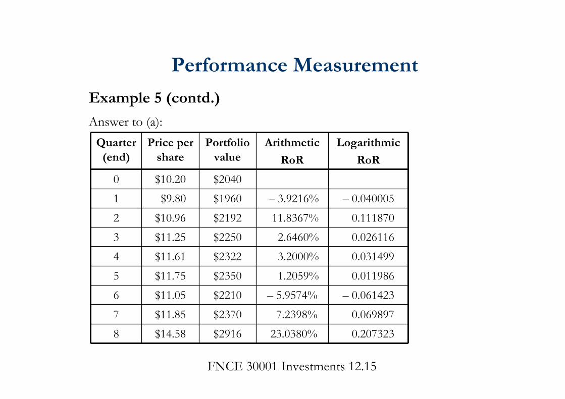
Example 5 (contd.)
Answer to (a):
Performance Measurement
Quarter (end)
Price per share
Portfolio value
Arithmetic
RoR
Logarithmic
RoR
0 $10.20 $20401 $9.80 $1960 – 3.9216% – 0.0400052 $10.96 $2192 11.8367% 0.1118703 $11.25 $2250 2.6460% 0.0261164 $11.61 $2322 3.2000% 0.0314995 $11.75 $2350 1.2059% 0.0119866 $11.05 $2210 – 5.9574% – 0.0614237 $11.85 $2370 7.2398% 0.0698978 $14.58 $2916 23.0380% 0.207323

FNCE 30001 Investments 12.16
Example 5 (contd.)Answer to (b):Total rates of return
Using arithmetic rates of return each quarter, we need the geometric rate of return over the 8 quarters:
Using logarithmic rates of return each quarter, we sum the quarterly returns:
Total Geometric RoR 0 960784 1 118367 1 230380 10 429412 (over 8 quarters). . ... ..
Performance Measurement
Total Logarithmic RoR 0 040005 0 111870 0 2073230 3572630 (over 8 quarters)
. . ... ..

FNCE 30001 Investments 12.17
Example 5 (contd.)Answer to (c):Mean rates of return
1 8
4
Mean Geometric RoR (pq) 1 429412 14 567007% pq
Mean Geometric RoR (pa) 1 04567007 119 558% pa
..
..
0 3572630Mean Logarithmic RoR (pq) 0 0446579 4 466% pa8
Mean Logarithmic RoR (pa) 0 0446579 417 863% pa
. . .
..
Performance Measurement

FNCE 30001 Investments 12.18
Example 5 (contd.)Three further observations on Example 5:Observation 1Of course, geometric and logarithmic rates of return are just different ways of telling the same story:
Observation 2Because there are no dividends, we can use just the start and end portfolio values and ignore the intermediate quarters.
0 3572630
0 0446579
Total Returns:
1 0 429412 (over 8 quarters)Mean Returns:
1 0 045670 pq
.
.
e .
e .
Performance Measurement

FNCE 30001 Investments 12.19
But, as we’ll see in Example 6, things can get more complex when there are dividends.
1 2
1 2
$2916Mean Geometric RoR 1$2040
1.429411765 119.558% pa
1 $2916Mean Logarithmic RoR n2 $20401 0.357263006217.863% pa
Performance Measurement
Example 5 (contd.)

FNCE 30001 Investments 12.20
Observation 3– The geometric rate of return is also known as the “time-
weighted rate of return”.• because every quarter (or other period) is given equal
weight in calculating the total and mean rates of return.– In many practical situations (like a mutual fund or a
superannuation fund) the size of the fund varies from time to time. “dollar-weighted rate of return”
Performance Measurement
Example 5 (contd.)

FNCE 30001 Investments 12.21
Example 6: One stock held for many periods; with dividendsAs in Example 5, except that we assume that dividends are paid and arereinvested in the same stock. The history of the stock unfolds as follows:
Quarter (end)
Price per share (ex-div)
Dividend per share
0 $10.201 $9.80 $0.082 $10.963 $11.25 $0.104 $11.615 $11.75 $0.156 $11.057 $11.85 $0.168 $14.58
Performance Measurement

FNCE 30001 Investments 12.22
Example 6 (contd.)
Qtr
(end)
Price ps
(ex-div)
Div ps Dividend
received
No. of shares bought
Holding Portfolio value
0 $10.20 200.000 $2040.001 $9.80 $0.08 x 200.000 = $16.00 / $9.80 = 1.633 201.633 $1976.002 $10.96 201.633 $2209.893 $11.25 $0.10 x 201.633 = $20.16 / $11.25 = 1.792 203.425 $2288.534 $11.61 203.425 $2361.765 $11.75 $0.15 x 203.425 = $30.51 / $11.75 = 2.597 206.022 $2420.766 $11.05 206.022 $2276.547 $11.85 $0.16 x 206.022 = $32.96 / $11.85 = 2.782 208.804 $2474.328 $14.58 208.804 $3044.36
Performance Measurement

FNCE 30001 Investments 12.23
Example 6 (contd.)We then calculate returns as usual using the portfolio values.Example 6 (contd.)
Quarter (end)
Portfolio value
Arithmetic
RoR
Logarithmic
RoR
0 $2040.001 $1976.00 – 3.1373% – 0.0318752 $2209.89 11.8367% 0.1118703 $2288.53 3.5584% 0.0349654 $2361.76 3.2000% 0.0314995 $2420.76 2.4978% 0.0246726 $2276.54 – 5.9574% – 0.0614237 $2474.32 8.6878% 0.0833098 $3044.36 23.0380% 0.207323
Performance Measurement
FNCE 30001 Investments 12.24
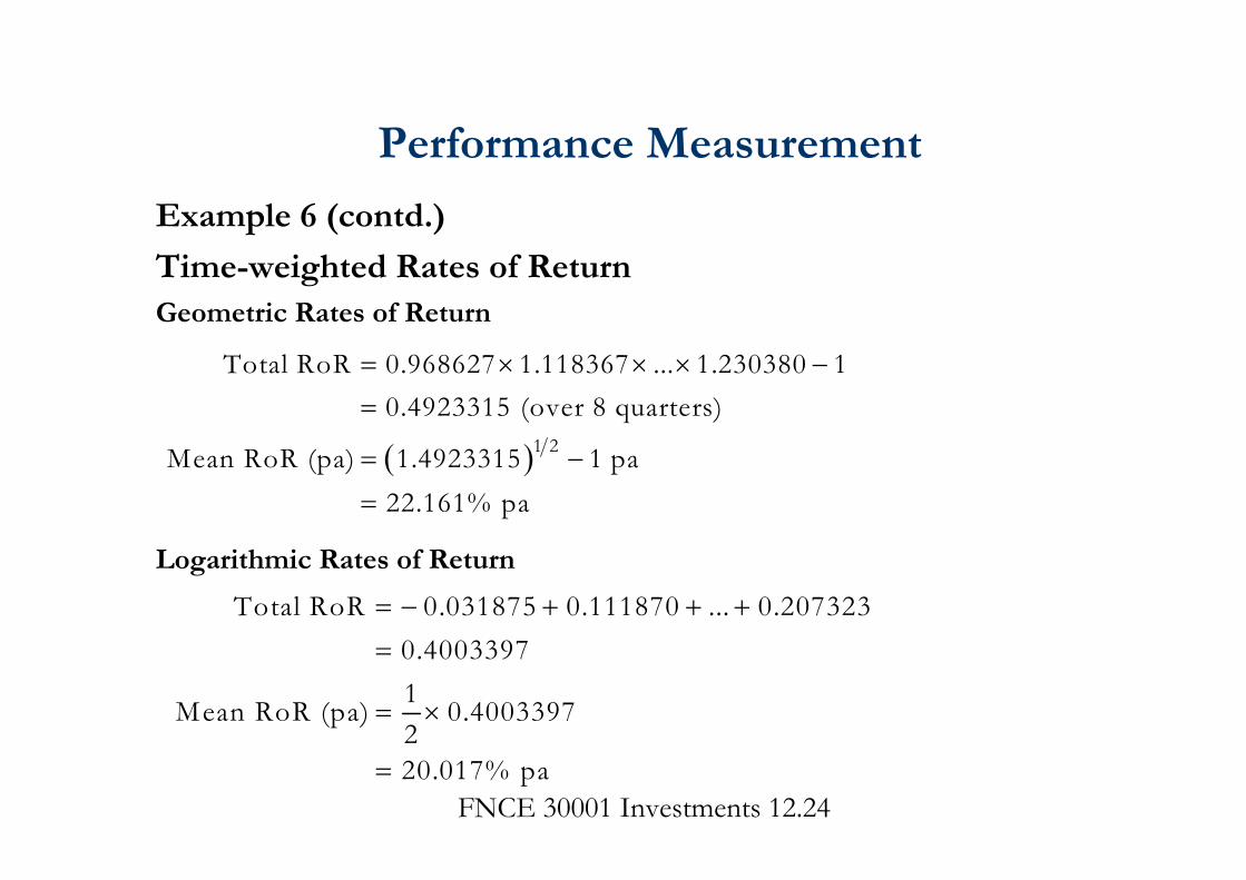
Example 6 (contd.)
Time-weighted Rates of ReturnGeometric Rates of Return
Logarithmic Rates of Return
1 2
Total RoR 0.968627 1.118367 ... 1.230380 10.4923315 (over 8 quarters)
Mean RoR (pa) 1.4923315 1 pa22.161% pa
Total RoR 0.031875 0.111870 ... 0.2073230.40033971Mean RoR (pa) 0.4003397220.017% pa
Performance Measurement

FNCE 30001 Investments 12.25
Example 6 (contd.)Again, using just the opening and closing portfolio values also works:
But we know the final portfolio value ($3044.36) only if we work through the reinvestment of dividends.
1 2
1 2
$3044.36M ean G eom etric RoR 1$2040.00
1.42933333 122.161% pa
1 $3044.36M ean Logarithm ic RoR n2 $2040.001 0.4003409220.017% pa
Performance Measurement

FNCE 30001 Investments 12.26
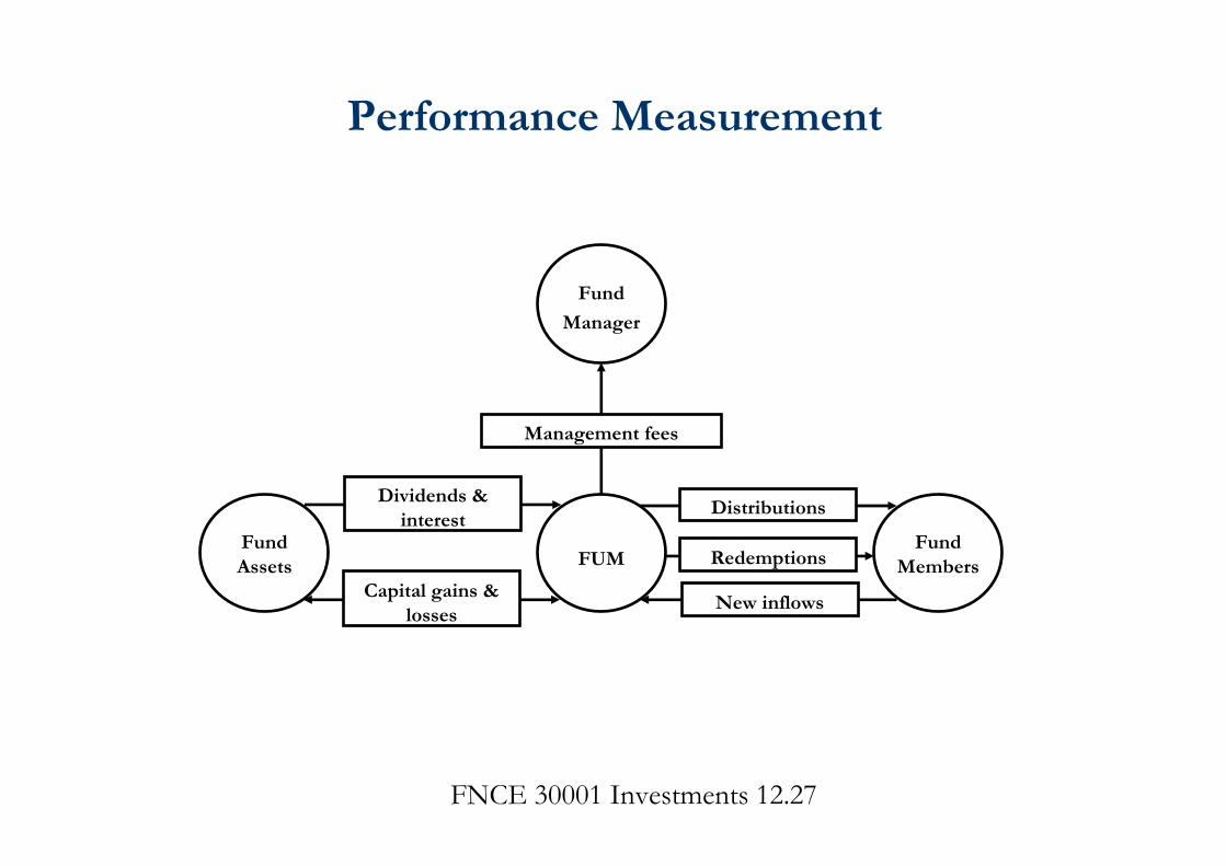
Example 7: Many stocks, many periods, with dividends, distributions, redemptions and new fund inflowsIn this example we consider the Melbourne Fund, which is an “open-ended” fund (eg a mutual fund or a superannuation fund) that invests in many stocks over many periods. Many of the stocks pay dividends. The Fund charges management fees.We assume that:– all cash flows occur at end-of-quarter (not during a quarter);– all cash flows are immediately reflected in the amount of
funds under management (FUM);– FUM is always measured at current market prices.
Performance Measurement
FNCE 30001 Investments 12.27
Performance Measurement
Fund Assets
Fund
Manager
FUMFund
Members
Management fees
Dividends & interest
Capital gains & losses
Distributions
Redemptions
New inflows

FNCE 30001 Investments 12.28
Example 7 (contd.)
ObjectiveWe wish to measure and report the mean rate of return pa (in discrete time) achieved by Fund members over the past 8 quarters.
We will measure and report on:• the time-weighted rate of return (TWR) and • the dollar-weighted rate of return (DWR).
Performance Measurement
FNCE 30001 Investments 12.29
Example 7 (contd.)
Effect of investing in many stocks– In principle, having many stocks instead of just one makes
little difference.– We simply sum the market values of all stocks held and all
dividends received.– But the practical record-keeping issues can be considerable.Distributions– Are like dividends paid from the Fund to fund members.– For tax reasons, distributions are often “pass-throughs” of
dividends received by the Fund.
Performance Measurement

FNCE 30001 Investments 12.30
Example 7 (contd.)Redemptions and new fund inflows– When fund members exit (“redemptions”) they are paid out
at a price that reflects the current market value of the Fund’s investments.
– Similarly, when new members join the Fund, or existing members increase their contributions, they do so at a price that reflects the current market value of the Fund’s investments.
Management fees– The Fund charges about 2.5% pa in management fees,
payable quarterly in arrears.
Performance Measurement

FNCE 30001 Investments 12.31
Example 7 (contd.)
Performance Measurement
Cash Flows of the Fund
Qtr (end)
Portfolio Value
(FUM) $m
Dividends received
$m
Capital gains $m
Distrib-utions
$m
Redemp-tions
$m
Manage-ment fees
$m
New inflows
$m
0 427.8
1 409.3 1.9 4.7 1.5 31.0 2.7 10.12 455.0 2.4 30.4 2.0 22.1 2.6 39.63 446.9 1.1 4.2 1.0 18.7 2.8 9.14 430.4 2.8 – 19.7 3.1 6.6 2.8 12.95 448.6 2.0 13.2 1.9 19.9 2.7 27.56 480.6 2.6 17.7 2.5 8.8 2.8 25.87 500.4 1.1 17.9 1.0 14.2 3.0 19.08 498.8 3.0 28.7 3.3 42.8 3.1 15.9

FNCE 30001 Investments 12.32
Example 7 (contd.)Note the identity here (using Quarters 0 and 1 as an example):
Funds under management at end Qtr 0 $427.8 mPlus Dividends received at end Qtr 1 + $1.9 mPlus Capital gains at end Qtr 1 + $4.7 mLess Distributions at end Qtr 1 – $1.5 mLess Redemptions at end Qtr 1 – $31.0 mLess Management fees at end Qtr 1 – $2.7 mPlus New inflows at end Qtr 1 + $10.1 mEquals Funds under management at end Qtr 1 $409.3 m
Performance Measurement

FNCE 30001 Investments 12.33
Example 7 (contd.)
Time-weighted Rate of Return (TWR)The after-fee dollar return to Fund members each quarter is given by:
Dollar return = Dividends + Capital gains – FeesThe rate of return each quarter is the dollar return divided by the funds under management at the end of the previous quarter. This is shown in the table on the next slide.These quarterly rates of return must then be accumulated over the 8 quarters and averaged.
Performance Measurement

FNCE 30001 Investments 12.34
Example 7 (contd.)
Qtr (end)
Portfolio Value (FUM)
$m
After-fee dollar return to Fund members
= dividends + capital gains – fees$m
Quarterly RoR
% pq
0 427.81 409.3 1.9 + 4.7 – 2.7 = 3.9 0.9116%
2 455.0 2.4 + 30.4 – 2.6 = 30.2 7.3785%
3 446.9 1.1 + 4.2 – 2.8 = 2.5 0.5495%
4 430.4 2.8 – 19.7 – 2.8 = – 19.7 – 4.4081%
5 448.6 2.0 + 13.2 – 2.7 = 12.5 2.9043%
6 480.6 2.6 + 17.7 – 2.8 = 17.5 3.9010%
7 500.4 1.1 + 17.9 – 3.0 = 16.0 3.3329%
8 498.8 3.0 +28.7 – 3.1 = 28.6 5.7154%
Performance Measurement
FNCE 30001 Investments 12.35
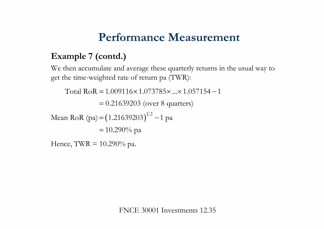
Example 7 (contd.)We then accumulate and average these quarterly returns in the usual way to get the time-weighted rate of return pa (TWR):
Hence, TWR = 10.290% pa.
1 2
Total RoR 1.009116 1.073785 ... 1.057154 10.21639203 (over 8 quarters)
Mean RoR (pa) 1.21639203 1 pa10.290% pa
Performance Measurement
FNCE 30001 Investments 12.36
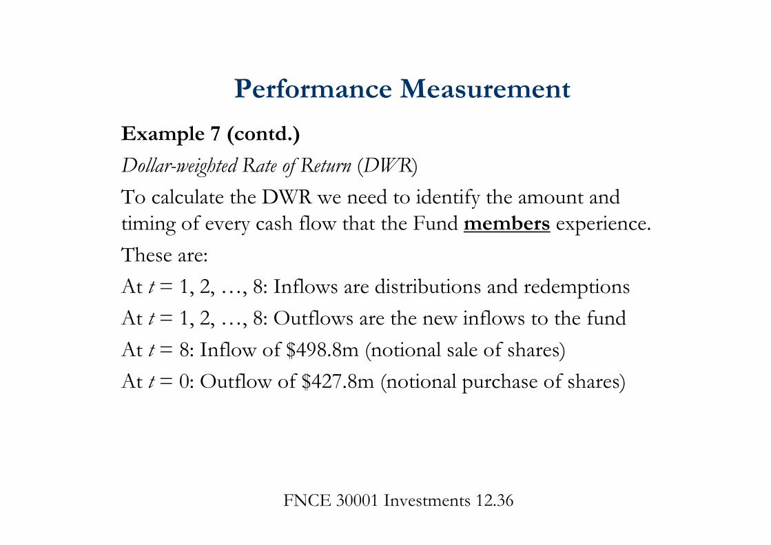
Example 7 (contd.)
Dollar-weighted Rate of Return (DWR)To calculate the DWR we need to identify the amount and timing of every cash flow that the Fund members experience.These are:At t = 1, 2, …, 8: Inflows are distributions and redemptionsAt t = 1, 2, …, 8: Outflows are the new inflows to the fundAt t = 8: Inflow of $498.8m (notional sale of shares)At t = 0: Outflow of $427.8m (notional purchase of shares)
Performance Measurement
FNCE 30001 Investments 12.37
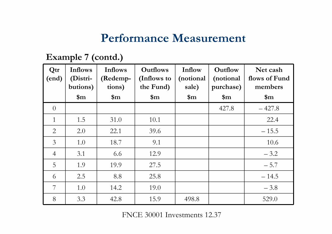
Example 7 (contd.)Qtr
(end)Inflows (Distri-butions)
$m
Inflows (Redemp-
tions)
$m
Outflows (Inflows to the Fund)
$m
Inflow (notional
sale)
$m
Outflow (notional purchase)
$m
Net cash flows of Fund
members
$m
0 427.8 – 427.81 1.5 31.0 10.1 22.42 2.0 22.1 39.6 – 15.53 1.0 18.7 9.1 10.64 3.1 6.6 12.9 – 3.25 1.9 19.9 27.5 – 5.76 2.5 8.8 25.8 – 14.57 1.0 14.2 19.0 – 3.88 3.3 42.8 15.9 498.8 529.0
Performance Measurement

FNCE 30001 Investments 12.38
Example 7 (contd.)Therefore we need to solve for i:
2 3 4 5
6 7 8
$22.4 $15.5 $10.6 $3.2 $5.71 1 1 1 1
$14.5 $3.8 $529 $427.8 0.1 1 1
The solution(found using Excel's IRR function) is 2.4902912% pq.The dollar-weighted rate of return pa is given by:
i i i i i
i i ii
41.024902912 1 10.339% pa.DWR
Performance Measurement

FNCE 30001 Investments 12.39
Example 7 (contd.)In this example there is little difference between time-weighted and dollar-weighted rates of return:
TWR = 10.290% paDWR = 10.339% pa
When intermediate cash flows are “small”, the two will be very close.When intermediate cash flows are “large” or when subperiod return is very volatile, then there can large differences.– If large amounts are contributed “just before” a period of
strong performance, then DWR will be greater than TWR.– If large amounts are withdrawn “ just before” a period of
strong performance, then DWR will be less than TWR.
Performance Measurement

FNCE 30001 Investments 12.40
Example 7 (contd.)
This example is our most realistic.But there are still further complications of reality that we won’t tackle, including:– Share capitalisation changes (eg bonus issues, rights issues,
reconstructions);– Cash flows that occur within subperiods (eg monthly cash
flows in a quarterly calculation);– Tax effects: eg What about imputation credits? What about
capital gains taxes?;– Out of date or even unobservable share prices.
Performance Measurement
FNCE 30001 Investments 12.41
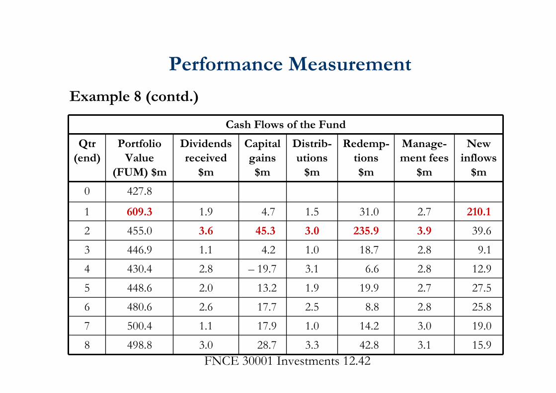
Example 8
As in Example 7, except there is now a large new inflow at the end of Quarter 1 followed by a large redemption at the end of Quarter 2. There are also some consequential changes to component cash flows (eg capital gains) – these are shown in redin the table on the next slide.
Because Quarter 2 has a high rate of return we should see a large increase in the dollar-weighted rate of return and little change in the time-weighted rate of return.
Performance Measurement
FNCE 30001 Investments 12.42
Example 8 (contd.)
Performance Measurement
Cash Flows of the Fund
Qtr (end)
Portfolio Value
(FUM) $m
Dividends received
$m
Capital gains $m
Distrib-utions
$m
Redemp-tions $m
Manage-ment fees
$m
New inflows
$m
0 427.8
1 609.3 1.9 4.7 1.5 31.0 2.7 210.1
2 455.0 3.6 45.3 3.0 235.9 3.9 39.63 446.9 1.1 4.2 1.0 18.7 2.8 9.14 430.4 2.8 – 19.7 3.1 6.6 2.8 12.95 448.6 2.0 13.2 1.9 19.9 2.7 27.56 480.6 2.6 17.7 2.5 8.8 2.8 25.87 500.4 1.1 17.9 1.0 14.2 3.0 19.08 498.8 3.0 28.7 3.3 42.8 3.1 15.9

FNCE 30001 Investments 12.43
Example 8 (contd.)
When we do the calculations, we find:TWR = 10.294% pa (vs 10.290% pa in Example 7) andDWR = 11.511% pa (vs 10.339% pa in Example 7).
That is, we find the expected result.
Performance Measurement

FNCE 30001 Investments 12.44
3. Performance Appraisal

FNCE 30001 Investments 12.45
The Fundamental Issue in Performance Appraisal• My portfolio has achieved a return of x%. Is this good or bad?• The fundamental issue is: good or bad compared to what?
– Answer: compared to the performance that might otherwise have been achieved.
– That is: an opportunity cost argument (alternative forgone).• But the “alternative forgone” must be in some sense comparable to
the investment actually made (“comparing apples with apples”).• Typically, this requirement is taken to mean having the same risk.• Therefore, performance appraisal requires us to use some kind of
asset pricing model, either explicitly or implicitly.
Performance Appraisal

FNCE 30001 Investments 12.46
• We need an asset pricing model to decide what is a “normal” (or expected) return.
• Any significant difference between actual performance and normal performance is “abnormal performance”.– If greater, then abnormally good:
• “superior performance” or “out-performance”.– If less, then abnormally bad:
• “inferior performance” or “under-performance”.• Why “significant difference”?
– Because actual performance may differ from normal performance randomly.
Performance Appraisal
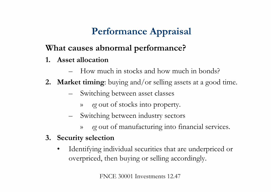
FNCE 30001 Investments 12.47
What causes abnormal performance?1. Asset allocation
– How much in stocks and how much in bonds?2. Market timing: buying and/or selling assets at a good time.
– Switching between asset classes » eg out of stocks into property.
– Switching between industry sectors» eg out of manufacturing into financial services.
3. Security selection
• Identifying individual securities that are underpriced or overpriced, then buying or selling accordingly.
Performance Appraisal

FNCE 30001 Investments 12.48
What causes abnormal performance? (contd.)4. Random influences (“luck”)
• Investment is an uncertain business, so it is always possible to get a good outcome (ex post) from a bad decision (ex ante)
– and, of course, vice versa.• We tend to label such outcomes as “good luck” and “bad
luck” respectively.• The effects of luck will on average wash out over time.
– Nevertheless, in any given case, a significance test may give a false positive or a false negative.
Performance Appraisal

FNCE 30001 Investments 12.49
• There is no universally accepted measure for performance appraisal.
• We will consider 7 approaches:1. Simple Benchmark Index2. The Sharpe Ratio 3. The Treynor Ratio4. Jensen’s Alpha5. The Information Ratio6. The M2 Measure7. Style Analysis
Performance Appraisal

FNCE 30001 Investments 12.50
1. Simple Benchmark Index– This is probably the most common approach.– We specify a benchmark index that has (or is assumed to
have) the same risk as the portfolio.– A benchmark index should also be:
• Viable; that is, could have been invested in.• Low transaction cost.• Identifiable before the fact.
Performance Appraisal

FNCE 30001 Investments 12.51
– eg a portfolio comprising mainly large listed Australian stocks might be benchmarked against the ASX’s All Ordinaries Accumulation Index.
– If the portfolio achieves a higher return than the index (it “beats the index”) then it has superior performance.
– Clearly, the bigger the difference the better the performance.
Performance Appraisal

FNCE 30001 Investments 12.52
• Good news:– Cheap to implement.– Easy to understand.– Doesn’t rely on any explicit asset pricing model
• which could also be bad news.• Bad news:
– No significance test.– How do we know the benchmark index (portfolio) has the
same risk as the portfolio?
Performance Appraisal

FNCE 30001 Investments 12.53
2. The Sharpe Ratio• Named after William Sharpe.• Fund (portfolio) risk is defined as the total risk of the portfolio:
– ie the standard deviation of portfolio returns.• The measure of return is the “excess return”, which is the
return above the risk-free rate.• It provides a measure of excess return per unit of total risk.• Also known as the “reward-to-variability ratio”.• There is a significance test due to Jobson and Korkie.
Performance Appraisal
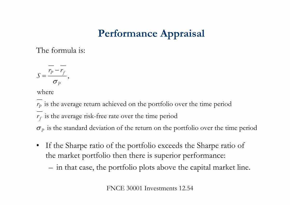
FNCE 30001 Investments 12.54
The formula is:
• If the Sharpe ratio of the portfolio exceeds the Sharpe ratio ofthe market portfolio then there is superior performance:– in that case, the portfolio plots above the capital market line.
,
where
is the average return achieved on the portfolio over the time period
is the average risk-free rate over the time period
is the standard deviation of the return on the portfolio o
P f
P
P
f
P
r rS
r
r
ver the time period
Performance Appraisal

FNCE 30001 Investments 12.55
Performance Appraisal

FNCE 30001 Investments 12.56
• Note that in this example the Fund’s return is less than the return on the market portfolio– BUT so is its risk (standard deviation).
• According to the Sharpe ratio, in this particular case the (much) lower risk more than compensates for the (slightly) lower return.
• Because the Sharpe ratio uses total risk, it is best suited to evaluating the performance of whole portfolios;– that is, when the portfolio to be evaluated is the total holding
of the investor.
Performance Appraisal
FNCE 30001 Investments 12.57
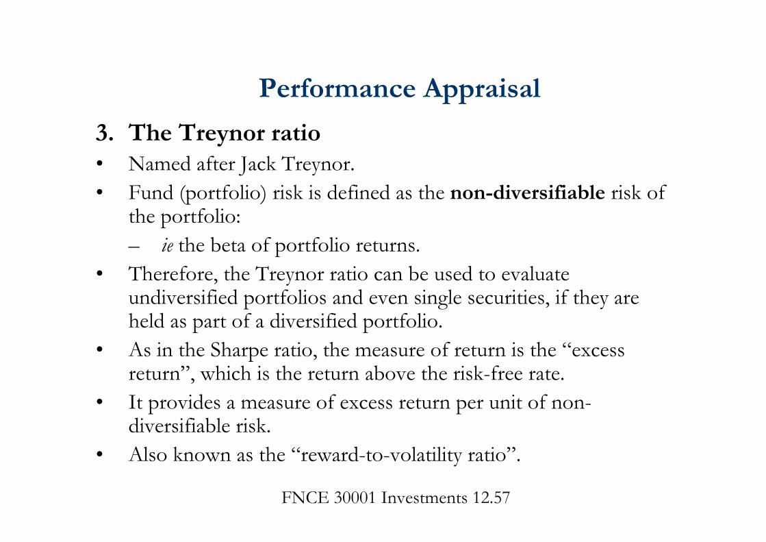
3. The Treynor ratio• Named after Jack Treynor.• Fund (portfolio) risk is defined as the non-diversifiable risk of
the portfolio:– ie the beta of portfolio returns.
• Therefore, the Treynor ratio can be used to evaluate undiversified portfolios and even single securities, if they areheld as part of a diversified portfolio.
• As in the Sharpe ratio, the measure of return is the “excess return”, which is the return above the risk-free rate.
• It provides a measure of excess return per unit of non-diversifiable risk.
• Also known as the “reward-to-volatility ratio”.
Performance Appraisal

FNCE 30001 Investments 12.58
The formula is:
,
where
is the average return achieved on the portfolio over the time period
is the average risk-free rate over the time period
is the beta of the portfolio over the time period
P f
P
P
f
P
r rT
r
r
Performance Appraisal

FNCE 30001 Investments 12.59
Performance Appraisal

FNCE 30001 Investments 12.60
• If the actual return on the portfolio exceeds the expected return on the portfolio (where “expected” means according to the CAPM) then there is evidence of superior performance.
• So the critical question is whether the Treynor ratio exceeds the market risk premium.
This means that E .
But E .
That is: .
which implies .
That is: Treynor ratio > the market risk premium.
P P
P f P M f
P f P M f
P fM f
P
r r
r r r r
r r r r
r rr r
Performance Appraisal

FNCE 30001 Investments 12.61
4. Jensen’s alphaNamed after Michael Jensen.Explicitly based on the CAPM.
Recall CAPM: E E
This is an single-period model.P f P M fr r r r
ex ante
Performance Appraisal
, , , ,Hence:
This is an multiperiod model.P t f t P M t f t tr r r r e
ex post
, , , ,Therefore: P t f t P M t f t tr r r r e
Note : No constant

FNCE 30001 Investments 12.62
So, if we insert a constant, αP , we expect its estimated value to be zero.
But suppose we run this regression and find that αP is significantly positive.Then, if the model is true, there is evidence of superior performance by the fund manager who chose portfolio P.Of course, if αP is significantly negative, this is evidence of inferior performance by the fund manager.And if αP is not significantly different from zero, there is no statistical evidence of abnormal performance by the fund manager.
, , , ,P t f t P P M t f t tr r r r e
Performance Appraisal

FNCE 30001 Investments 12.63
• Note: By definition, we can calculate Jensen’s alpha as follows:
• But where does the βP come from?• From the regression!
• And, having done the regression, we also get the prob value (significance level) for the hypothesis that αP equals zero.
• So the bottom line is: do the regression!
, , , ,
, , , ,
P P t f t P M t f t
P t f t P M t f t
r r r r
r r r r
Performance Appraisal
FNCE 30001 Investments 12.64
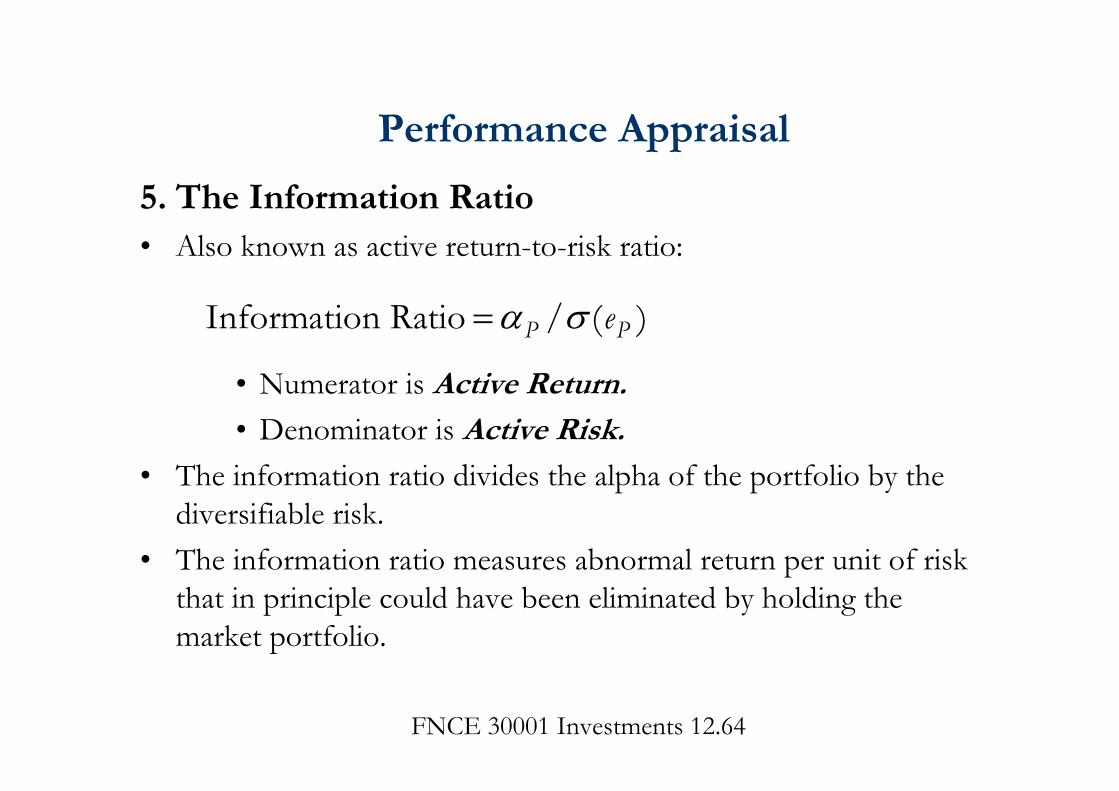
5. The Information Ratio• Also known as active return-to-risk ratio:
• Numerator is Active Return.• Denominator is Active Risk.
• The information ratio divides the alpha of the portfolio by the diversifiable risk.
• The information ratio measures abnormal return per unit of risk that in principle could have been eliminated by holding the market portfolio.
Information Ratio / ( )P Pe
Performance Appraisal

FNCE 30001 Investments 12.65
6. The M2 Measure• Popularised by Franco Modigliani and his granddaughter Leah
Modigliani.• A selected portfolio, P, will nearly always have a return and
standard deviation that differ from the return and standard deviation of the market portfolio, M.
• But we can combine P and the risk-free asset to make a new portfolio, P*, that has the same standard deviation (but different return) as the market portfolio, M.
• Since both P* and M have the same risk (standard deviation), we can validly compare their returns.– The difference between these returns is the M2 measure.
• If the return on P* exceeds the return on M, then P has superior performance.
Performance Appraisal

FNCE 30001 Investments 12.66
Performance Appraisal

FNCE 30001 Investments 12.67
Example
*
*
*
Suppose 6%, 10%, 15%, 45% and 3%.
Recall that for a two-asset portfolio, where one of the assets is risk-free:.
We require 45%.45%Therefore 4.510%
and 1 1 4
P P M M f
P P P
P M
MPP
P P
f P
r r r
w
w
w w .5 3.5.
This means that for every $1 of our own invested, we borrow $3.50 and invest the whole amount ($4.50) in portfolio .What is the return on portfolio * ?And is this return greater than the retu
PP
rn on portfolio ?M
Performance Appraisal

FNCE 30001 Investments 12.68
Example (contd.)
*
2*
2
The return on portfolio * is given by
4.5 6% 3.5 3%16.5%
Recall that 15%.
Therefore 16.5% 15% 1.5%.
Because is greater than zero, superior performance is indicated.
P P P f f
M
P M
Pr w r w r
r
M r r
M
Performance Appraisal

FNCE 30001 Investments 12.69
7. Style Analysis• Introduced by William Sharpe (1992).• Can be considered a 7th type of performance appraisal.
– But is a bit more than that.• Consider two-stage “top down” portfolio construction:
1. Allocation between major asset classes (“styles”):• eg stocks (equities) vs long-term debt (bonds) vs short-
term debt (bills)2. Security selection:
• Which securities to buy within each asset class.
Performance Appraisal

FNCE 30001 Investments 12.70
• The objective of style analysis is to measure– how much of a portfolio’s return is due to style choice (asset
allocation) vs– how much is due to other factors including selection.
• Suppose we observe the monthly returns on a portfolio over a period of, say, 5 years.– The managers of the portfolio are not permitted to short sell
or borrow.– They can invest in equities (E), long-term debt (L) and short-
term debt (S).• That is, there are 3 asset classes (E, L and S).
Performance Appraisal

FNCE 30001 Investments 12.71
• Then we specify the following regression equation:
Performance Appraisal
, , , ,
where is the return in month means the portfolio means an index of investments in equities means an index of investments in long-term debtmeans an index of inves
P t E E t L L t S S t t
t
r r r r e
r tPELS
tments in short-term debt

FNCE 30001 Investments 12.72
But we also have the following restrictions:0 10 10 1
1So we incorporate these restrictions into our regression estimation.
E
L
S
E L S
Performance Appraisal

FNCE 30001 Investments 12.73
2
Suppose we find:0.0021 0.86 0.11 0.03
and the regression is 0.92and the constant (0.0021) is significantly different from zero.What do these findings mean?
P E L Sr r r r
R
Performance Appraisal

FNCE 30001 Investments 12.74
Observations:1. The selected portfolio behaves like one (the “tracking
portfolio”) that consists largely (86%) of equities.2. 92% of the variation in portfolio return is attributable to asset
allocation (style)• which leaves only 8% being attributable to timing and
security selection.3. Nevertheless, abnormal performance is 0.21% per month
(about 2.5% pa) and is statistically significant.
Performance Appraisal

FNCE 30001 Investments 12.75
4. Performance Attribution

FNCE 30001 Investments 12.76
• Many fund managers specify a benchmark portfolio against which their performance should be assessed.– eg the ASX 200 or the S&P 500.
• The difference between the portfolio return and the benchmark return is the measure of under- or out-performance.
• Many fund managers also say they undertake a two-stage (“top down”) analysis:1. Asset allocation2. Stock selection
• The inevitable question: how much of the under- or out-performance was due to asset allocation and how much was due to stock selection?– This is “performance attribution”.
Performance Attribution

FNCE 30001 Investments 12.77
• Suppose the benchmark is the ASX 200.• To keep this simple let’s say the ASX 200 consists of 3 asset
classes:– Shares in mining and energy companies (M)– Shares in banks and financial companies (F)– Shares in industrial and other companies (I)
• So the return on the benchmark is:
where ( ) is the return on the index of mining companies
and is the weight given to mining companies in the ASX 200.
M M F F I IB B B B B B B
MB
MB
r w r w r w r
eg r
w
Performance Attribution

FNCE 30001 Investments 12.78
• The return that the Fund’s portfolio (P) achieved is:
• Let’s compare these equations:
w here ( ) is the return on the m in ing com panies chosen by the Fund
and is the w eight g iven to m in ing com paniesin the Fund's portfo lio .
M M F F I IP P P P P P P
MP
MP
r w r w r w r
eg r
w
Performance Attribution
M M F F I IB B B B B B B
M M F F I IP P P P P P P
r w r w r w r
r w r w r w r
FNCE 30001 Investments 12.79
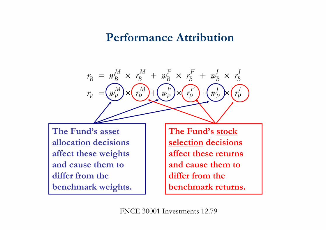
M M F F I IB B B B B B B
M M F F I IP P P P P P P
r w r w r w r
r w r w r w r
The Fund’s asset allocation decisions affect these weights and cause them to differ from the benchmark weights.
The Fund’s stock selection decisions affect these returns and cause them to differ from the benchmark returns.
Performance Attribution

FNCE 30001 Investments 12.80
Performance Attribution
Let’s look just at one of the asset classes (say, class I).
FNCE 30001 Investments 12.81
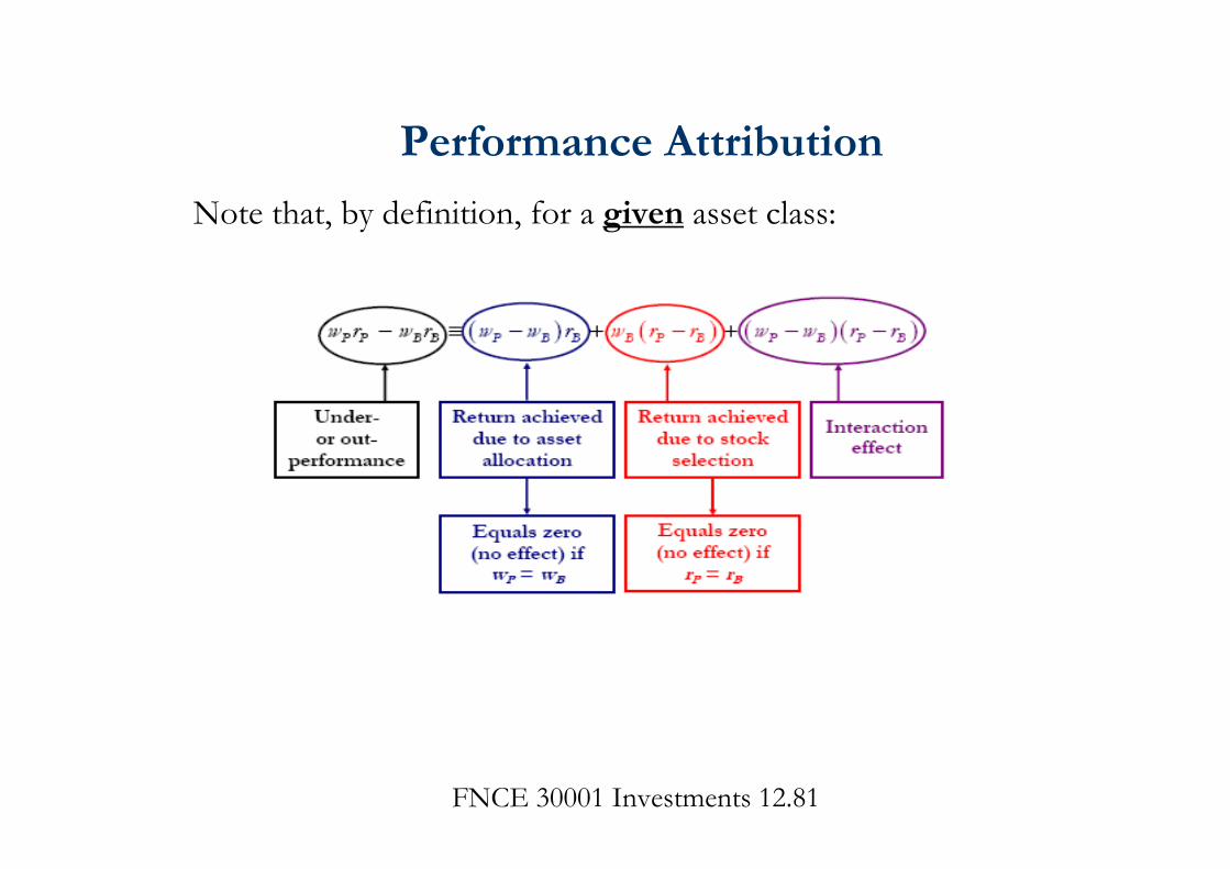
Note that, by definition, for a given asset class:
Performance Attribution

FNCE 30001 Investments 12.82
• This equation is used for each asset class.• The result for the portfolio as a whole is found by then summing
across all asset classes.
Performance Attribution
Recommended