Fluid Mechanics
Indian Institute of Technology, Kanpur
Prof. Viswanathan Shankar
Department of chemical Engineering
Lecture No. # 02
Welcome to this second lecture on this course on fluid mechanics, designed for chemical
engineering undergraduate students. In the 1st lecture, I laid out the motivations as to
why fluid mechanics is very important in chemical process industries by showing various
examples.
(Refer Slide Time: 00:39)
For example, we will try to show, that fluid mechanics in chemical process industries. It
can come in various forms, so there are some cases in which the role of fluid mechanics
is direct, so let me say direct role, as in the case of pumping of fluids, that is there in all
process industries; secondly, you have pumping and transportation. Secondly, you have
flow measurement. Thirdly, we saw, that mixing an agitation of reactors in chemical
reactors. Fourthly, we saw, that the design of packed and fluidized beds. These are some
examples where fluid mechanics plays a direct role in the design of chemical process
equipment, as well as, various unit operations, that involve in detail the nature of fluid
flow.
There are cases where fluid mechanics is important, but plays an indirect role where the
goal is not fluid for per say, in the sense, that there are, there are some other unit
operations, that are happening. For example, heat transfer in heat exchanger equipment
or for example, you could have a bubble column reactor, where reaction is happening
between the gas phase and liquid phase there.
The role of fluid mechanics is important, but it is slightly indirect because there, the role
of the fluid is to bring the reactant from a place to a point of interest. For example, if you
have a catalyst particle, we saw in the last lecture, and you, this could be, for example, a
catalyst particle in a packed bed reactor.
If you take an individual catalyst particle, you have fluid flow around it like this. So, the
role of fluid flow is to bring the reactant from this point close to the surface, so that
reaction can take place. Here, the detailed nature of flow is very important and if the
flow is slightly different, for example, like, so if there are recirculating zones in the end
of the cylinder or, or surface, so this really determines whether the product is taken away
and how fast the product is taken away as compared to this case. So, the detailed nature
of flow is important in most unit operations; is important in most unit operations.
The fundamental reason is that in chemical industry most of the operations are carried
out with fluid as the carrying medium, that is, that is primarily because handling fluids
and pumping fluids is easier and mixing fluids is easier and diffusion rates are much
faster in a fluid. So, for these reasons, for these fundamental reasons, most processing
happens typically in the fluid phase, even though the final product need not be in the
fluid form. Final product could be a powder of a pharmaceutical, but the processing itself
happens largely in the fluid phase.
So, fluid mechanics, as we saw in the last lecture and as I am reviewing here, plays the
fundamental role in many chemical processing industries and equipment.
(Refer Slide Time: 04:53)
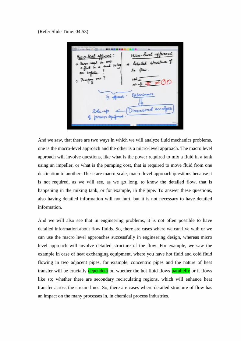
And we saw, that there are two ways in which we will analyze fluid mechanics problems,
one is the macro-level approach and the other is a micro-level approach. The macro level
approach will involve questions, like what is the power required to mix a fluid in a tank
using an impeller, or what is the pumping cost, that is required to move fluid from one
destination to another. These are macro-scale, macro level approach questions because it
is not required, as we will see, as we go long, to know the detailed flow, that is
happening in the mixing tank, or for example, in the pipe. To answer these questions,
also having detailed information will not hurt, but it is not necessary to have detailed
information.
And we will also see that in engineering problems, it is not often possible to have
detailed information about flow fluids. So, there are cases where we can live with or we
can use the macro level approaches successfully in engineering design, whereas micro
level approach will involve detailed structure of the flow. For example, we saw the
example in case of heat exchanging equipment, where you have hot fluid and cold fluid
flowing in two adjacent pipes, for example, concentric pipes and the nature of heat
transfer will be crucially dependent on whether the hot fluid flows parallelly or it flows
like so; whether there are secondary recirculating regions, which will enhance heat
transfer across the stream lines. So, there are cases where detailed structure of flow has
an impact on the many processes in, in chemical process industries.
So, we will in this course discuss both, macro level approaches, as well as, micro level
approaches in equal measure. And both have their own successes and both have their
own limitations, as we will have opportunity to point out all through this course.
There is another important approach, that, that sort of complements the, these two
approaches, that is, the third approach, which complements the macro and micro level
approaches. This is experimentation, experimental observation. This is because it is not
often possible to analyze all problems, that occur in engineering applications using a
fundamental approach, either microscopic or macro level approaches. In many cases we
have to do systematic experiments to understand a given process equipment, for
example, like a packed bed or a fluidized bed and so on, where it is not really possible to
understand everything from first principles. So, experiments play a major role in
engineering design, especially in process industries.
And here we will show, that by judicious use of dimensional analysis, experiments can
be made much more, doing experiments can be made in a very rational way and we can
collect data and present them in a very, very economical way. And dimensional analysis
has also very, very important applications in scale up of process equipment, as we will
have opportunities to discuss later. So, this is roughly the, these are the kind of
approaches, that we are going to take as, as we go long in this course, but as an engineer
it is important to have a balance mix of all three.
So, ideally, we would like to solve all problems as fundamentally as possible, using first
principles approach, that is, the micro-scale approach, where we compute the detailed
flow field everywhere in the flow. But where it is not possible to have such an approach,
we have to settle for a macroscopic approach where we will see, that we need a lot of
experimental input. So, the macroscopic approach and the experimental approach go
hand in hand, where some parts of this analysis can be done using the macro-approach,
but certain inputs are required from experimental data in the macroscopic approach. So,
we will have opportunities to discuss, opportunity to discuss all the three approaches as
we go along.
(Refer Slide Time: 09:51)
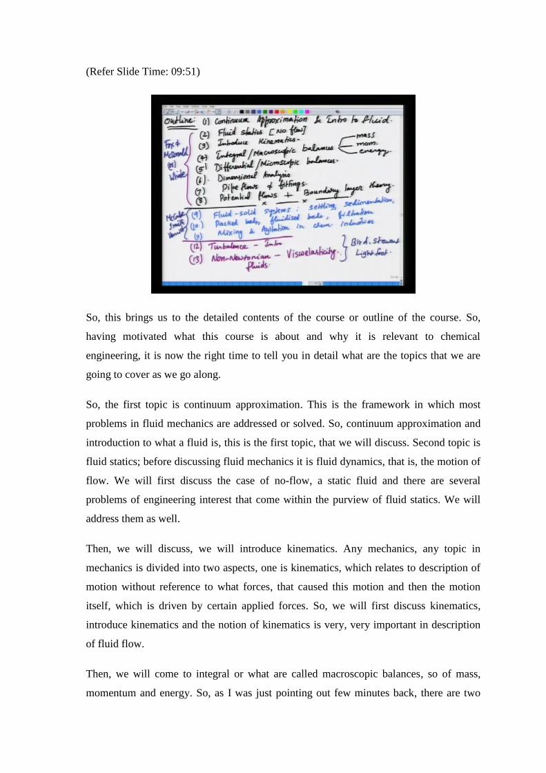
So, this brings us to the detailed contents of the course or outline of the course. So,
having motivated what this course is about and why it is relevant to chemical
engineering, it is now the right time to tell you in detail what are the topics that we are
going to cover as we go along.
So, the first topic is continuum approximation. This is the framework in which most
problems in fluid mechanics are addressed or solved. So, continuum approximation and
introduction to what a fluid is, this is the first topic, that we will discuss. Second topic is
fluid statics; before discussing fluid mechanics it is fluid dynamics, that is, the motion of
flow. We will first discuss the case of no-flow, a static fluid and there are several
problems of engineering interest that come within the purview of fluid statics. We will
address them as well.
Then, we will discuss, we will introduce kinematics. Any mechanics, any topic in
mechanics is divided into two aspects, one is kinematics, which relates to description of
motion without reference to what forces, that caused this motion and then the motion
itself, which is driven by certain applied forces. So, we will first discuss kinematics,
introduce kinematics and the notion of kinematics is very, very important in description
of fluid flow.
Then, we will come to integral or what are called macroscopic balances, so of mass,
momentum and energy. So, as I was just pointing out few minutes back, there are two
approaches that are largely taken in addressing fluid flow problems, one is the macro-
scale approach where the detailed flow structure is not required and the integral balances
are one way of addressing such problems using integral balance, using macroscopic
balance of mass, momentum and energy. And then, we will go to differential balances or
microscopic balances of mass, momentum and energy. As the name suggests, integral
balances will involve integrals of various quantities, such as mass, momentum, energy
and how they change in a flow while differential balances will involve differential
equations of these quantities, like mass, momentum and energy. And finally, these
differential equations will be valid at each and every point in the fluid and if you can
solve them, this will be the most, you know, detailed information, that one can have for a
fluid flow.
After we do, do that we will do dimensional analysis and then apply this to pipe flows
and fittings. And then we will do, we will see, that fluid flow is normally characterized
by a single parameter. Once we do dimensional analysis, there is a parameter called
Reynolds number, which will recur throughout this course after we, we are done with the
basics. So, the Reynolds number, when it is small the flow speeds are small; when the
Reynolds number, when it is large the flow speeds are very large. So, when the flow
speeds are very large we will deal with what are called potential flows. These are some
approximations of the full microscopic equations, differential equations of flow.
And we will discuss, that when potential flow fails we have to invoke, what is called,
boundary layer theory. This is a very important topic in fluid mechanics. Once we are
done with this, this roughly concludes the basic aspects of fluid mechanics.
So, then we will go to fluid solid systems, this involves chemical engineering
applications such as settling, sedimentation, and so on. Then, we will proceed to the
analysis of packed beds, fluidized beds and filtration. We will then proceed to mixing an
agitation in chemical, in chemical industries. So, these are some of the primary
applications of fluid mechanics in chemical processing industries.
And then we will find that finally, we will go to slightly fundamental, but advanced
topics, which are unique to chemical, chemical industries. One is usually the flows, that
we encounter in chemical industries, are not very simple. For example, the flow will not
happen at a very slow pace, it will happen at a very rapid flow rate. In such cases the
flow will become turbulent, so we will give a brief introduction to turbulence and derive
some basic equations of turbulent flows, so that will be the next part.
And finally, we will discuss non-Newtonian flows; I will discuss what these are as we go
along. Simple fluids like water and air called Newtonian fluids because they behave in a
particular way, whereas many complex fluids that are, many fluids, that are encountered
in chemical industry, for example they may be slurries or suspensions of one particle in
another or dispersions of one liquid in another and so on. These are very complex
systems and the way in which they behave in there flow is very different from how water
and air behave. So, these are non-Newtonian fluids or since they exhibit some elasticity
in additions to viscous effects, they are called viscoelastic fluids. So, we will give a brief
introduction to non-Newtonian fluids.
So, this is the agenda for this course and I have already told you the texts that are
suggested for additional readings. Although all these material will be inherently self-
contained, so I have already mentioned this to you, that the basic parts of this course up
to these will, for example you can follow Fox and McDonald for additional reading or
White. Fluid mechanics for these, in addition to the lecture notes, you can follow
McCabe, Smith and Harriet. For these, you can follow Bird, Stewart and Lightfoot
transport phenomena. So, this is the rough agenda for this course.
(Refer Slide Time: 17:51)
-----------------------------------------------------------------------------------------------------------
Equations:
-----------------------------------------------------------------------------------------------------------
-----------------------------------------------------------------------------------------------------------
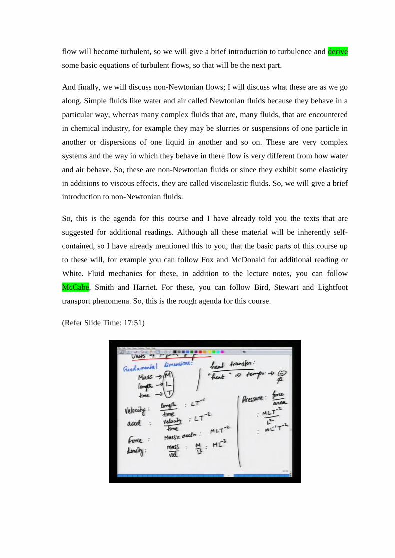
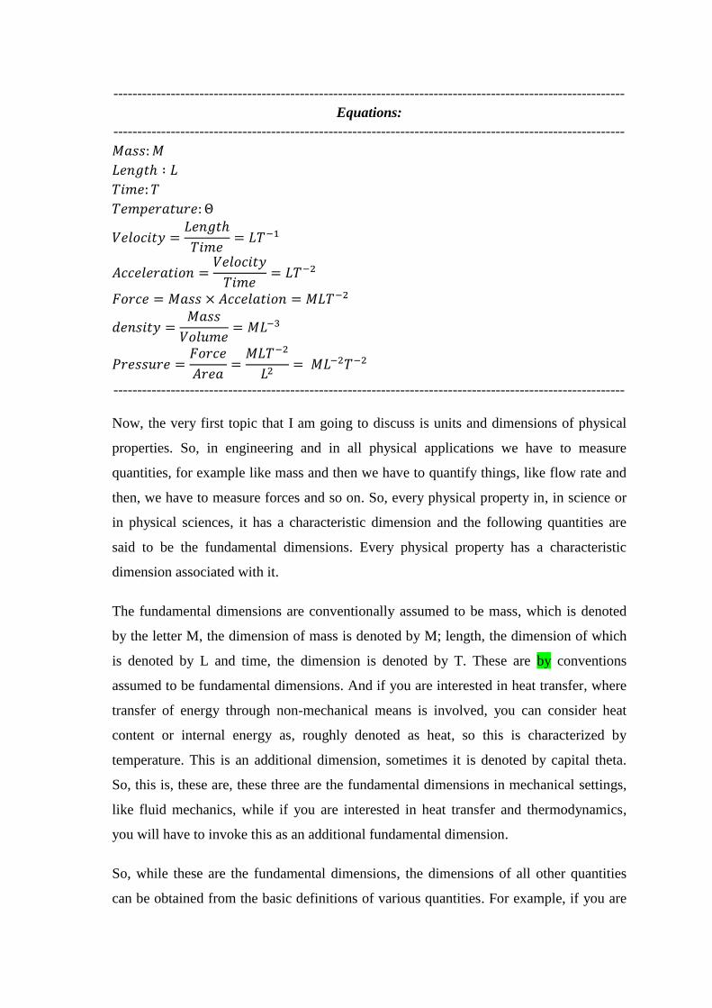
Now, the very first topic that I am going to discuss is units and dimensions of physical
properties. So, in engineering and in all physical applications we have to measure
quantities, for example like mass and then we have to quantify things, like flow rate and
then, we have to measure forces and so on. So, every physical property in, in science or
in physical sciences, it has a characteristic dimension and the following quantities are
said to be the fundamental dimensions. Every physical property has a characteristic
dimension associated with it.
The fundamental dimensions are conventionally assumed to be mass, which is denoted
by the letter M, the dimension of mass is denoted by M; length, the dimension of which
is denoted by L and time, the dimension is denoted by T. These are by conventions
assumed to be fundamental dimensions. And if you are interested in heat transfer, where
transfer of energy through non-mechanical means is involved, you can consider heat
content or internal energy as, roughly denoted as heat, so this is characterized by
temperature. This is an additional dimension, sometimes it is denoted by capital theta.
So, this is, these are, these three are the fundamental dimensions in mechanical settings,
like fluid mechanics, while if you are interested in heat transfer and thermodynamics,
you will have to invoke this as an additional fundamental dimension.
So, while these are the fundamental dimensions, the dimensions of all other quantities
can be obtained from the basic definitions of various quantities. For example, if you are
worried about velocity, because in fluid mechanics we will have to worry about velocity
a lot, it is a rate at which fluid flows per unit time, rate at which displacement of a fluid
changes per unit time. So, it has dimensions of L, length over time, LT to the minus 1.
So, acceleration of a fluid is the rate at which velocity changes, so velocity is rate at
which displacement changes per time, acceleration is rate of velocity. So, it is velocity by
time, so it becomes LT to the minus 2 and then force is, from Newton’s second law,
mass times acceleration, mass times acceleration, so MLT to the minus 2.
So, one can derive units of density and so on, density is mass divided by volume, it is
mass of a, mass of a fluid per unit volume, it is M by L cube, it is, volume has a
dimensions of length cube, so it is ML to the minus 3. And so, one could derive pressure
in, as is defined as the force, that is acting normally per unit area. So, we will divide
force MLT to the minus 2 by L squared, area has dimensions of length squared, so it is
ML to the minus 1 T to the minus 2 and so on. So, these are dimensions, these are
fundamentally ascribed to all physical quantities there are.
(Refer Slide Time: 21:46)
-----------------------------------------------------------------------------------------------------------
Equations:
-----------------------------------------------------------------------------------------------------------
Length: meter or cm
Time: sec or min or hr
-----------------------------------------------------------------------------------------------------------
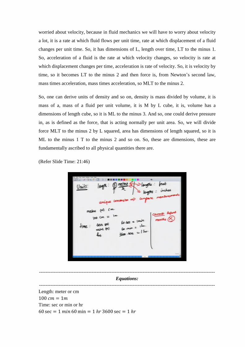
These are very unique, but units are human constructs, so whenever you measure a
physical quantity you have to accept a convention. For example, if you measure length
you have to use meters or centimeters or feet, or whatever you want. So, different people
can measure the same dimension differently and they will report the number. For
example, length is reported as 5 meters, these are the units and the numbers specify the
numerical value with which length is the amount of length, that is present in that
particular measurement in terms of the unit that has been chosen. For example, 5 meters,
so the dimensions of all physical, of various physical quantities are unique, but units are
not, units are basically means of characterizing or measuring various physical quantities,
and as long as, even if one uses different, for example, somebody else measures lengths
in feet and somebody else measure lengths in, in, in inches or so on, as long as you can
convert from one to another in a unique way. If you have unique conversion rows that
mean that you can compare measurements, various measurements.
So, units are not fundamental, as fundamental as dimensions; units are merely a
convention that everybody agrees to work on. So, if a certain group of people agree to
work with some set of units and some other group decide to work on some other set of
units, as long as, these two groups agree on the conversion between one’s, one units to
another, there both the measurements can be compared. You can be convert, you can, it
can be converted. So, there must be a unique relation between one set of units to another.
For example, you can measure lengths in terms of meters or centimeters and with the
conversion rule, that 100 centimeter is 1 meter and so on. So, time is measured, time can
be measured in seconds, minutes or hours; seconds or minutes or hours. With the unique
conversion rule, that 60 seconds is 1 minute, 60 minutes is 1 hour and so on. Therefore,
3600 seconds is 1 hour. However, you cannot measure time in months or report time in
months because there is no unique conversion between months and all these fundamental
units, like minutes or hours or seconds. So, cannot report time in months, that is not
correct because there is no precise conversion factor between months and, and the
fundamental unit, like second, minutes or hours.
(Refer Slide Time: 25:20)
-----------------------------------------------------------------------------------------------------------
Equations:
-----------------------------------------------------------------------------------------------------------
SI units:
Length: meter (m)
Mass: kilogram (kg)
Time: seconds (s)
Temperature: Kelvin (K)
Derived units:
Velocity:
Accleration:
Force:
Pressure:
Work:
Power:
-----------------------------------------------------------------------------------------------------------
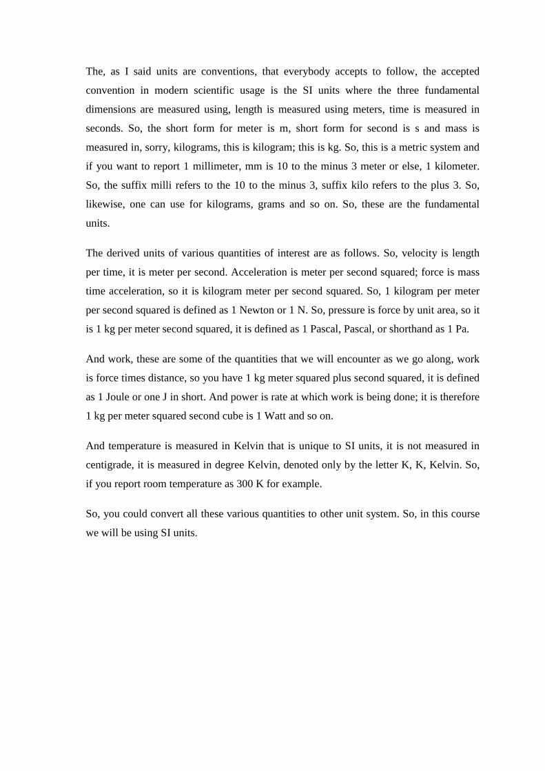
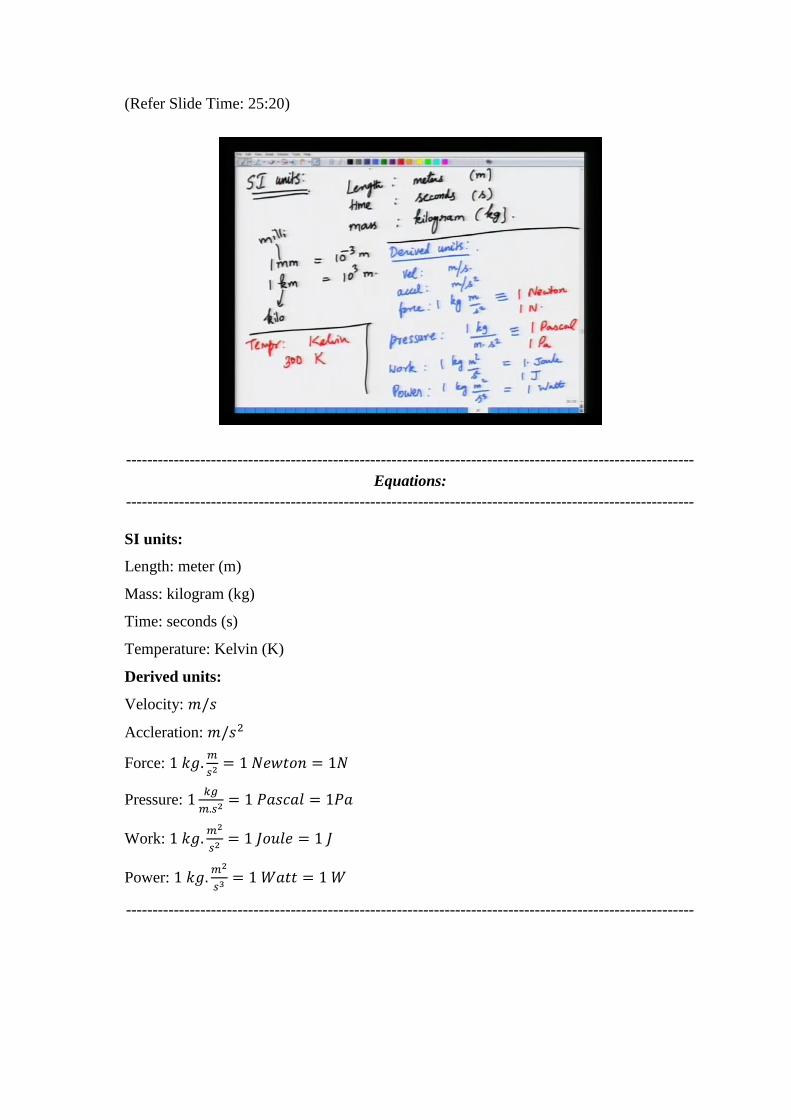
The, as I said units are conventions, that everybody accepts to follow, the accepted
convention in modern scientific usage is the SI units where the three fundamental
dimensions are measured using, length is measured using meters, time is measured in
seconds. So, the short form for meter is m, short form for second is s and mass is
measured in, sorry, kilograms, this is kilogram; this is kg. So, this is a metric system and
if you want to report 1 millimeter, mm is 10 to the minus 3 meter or else, 1 kilometer.
So, the suffix milli refers to the 10 to the minus 3, suffix kilo refers to the plus 3. So,
likewise, one can use for kilograms, grams and so on. So, these are the fundamental
units.
The derived units of various quantities of interest are as follows. So, velocity is length
per time, it is meter per second. Acceleration is meter per second squared; force is mass
time acceleration, so it is kilogram meter per second squared. So, 1 kilogram per meter
per second squared is defined as 1 Newton or 1 N. So, pressure is force by unit area, so it
is 1 kg per meter second squared, it is defined as 1 Pascal, Pascal, or shorthand as 1 Pa.
And work, these are some of the quantities that we will encounter as we go along, work
is force times distance, so you have 1 kg meter squared plus second squared, it is defined
as 1 Joule or one J in short. And power is rate at which work is being done; it is therefore
1 kg per meter squared second cube is 1 Watt and so on.
And temperature is measured in Kelvin that is unique to SI units, it is not measured in
centigrade, it is measured in degree Kelvin, denoted only by the letter K, K, Kelvin. So,
if you report room temperature as 300 K for example.
So, you could convert all these various quantities to other unit system. So, in this course
we will be using SI units.
(Refer Slide Time: 29:07)
-----------------------------------------------------------------------------------------------------------
Equations:
-----------------------------------------------------------------------------------------------------------
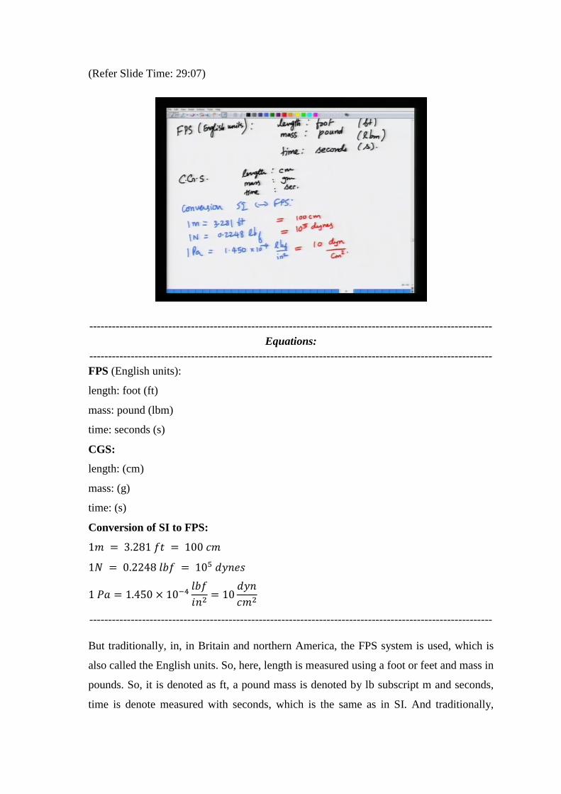
FPS (English units):
length: foot (ft)
mass: pound (lbm)
time: seconds (s)
CGS:
length: (cm)
mass: (g)
time: (s)
Conversion of SI to FPS:
-----------------------------------------------------------------------------------------------------------
But traditionally, in, in Britain and northern America, the FPS system is used, which is
also called the English units. So, here, length is measured using a foot or feet and mass in
pounds. So, it is denoted as ft, a pound mass is denoted by lb subscript m and seconds,
time is denote measured with seconds, which is the same as in SI. And traditionally,
people have also used centimeter-gram-second, where length is in centimeter, mass is in
gram and time in seconds.
So, if you look at various text books or some other tables, they will tell you how to
convert from one system of unit to others, although in this course we will follow only the
SI units. It is sometimes useful if you read literature or text books where they follow
some other units; you should be able to convert those units to the SI units. So, for
example, 1 meter, so I am just giving you some examples, conversion, so SI to FPS, so 1
meter is 3.281 feet and so on. You have this conversion and 1 Newton is 0.2248, the unit
for force is pound force lb f and 1 Pascal is 1.450 into 10 to the minus 4 lb f per inch
squared and so on. So, for example, 1 meter is 100 centimeter, if you were to convert this
to CGS units; 1 Newton force is 10 to the power 5 dynes, this is equal to; 1 Pascal is 10
dynes per centimeter squared and so on.
So, one should be able to convert from one form of units to other by looking up a text
books or tables, but in this course we will follow only SI units; that, is the accepted
system of units.
(Refer Slide Time: 31:56)
-----------------------------------------------------------------------------------------------------------
Equations:
-----------------------------------------------------------------------------------------------------------
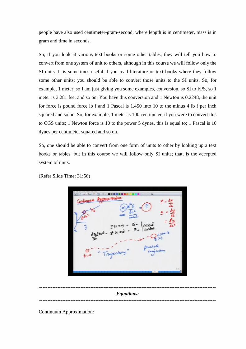
Continuum Approximation:
Initial conditions:
-----------------------------------------------------------------------------------------------------------
So, then, so having discussed the fundamental definition of dimensions of various
quantities, we are ready to understand what a fluid is. So, firstly, before understanding
what a fluid is we have to introduce the framework with which we are going to
understand fluid flows, the framework with which fluid flows are normally understood, it
is called the continuum approximation.
So, let me describe in detail what this approximation is. Many of you must have dealt
with or read courses, had courses on mechanics of point particles in your physics classes.
There, of course you are interested, for example, in motion of a point particle under the
influence of some forces. So, the fundamental equation, that describes the motion of
point particles is the Newton’s 2nd law of motion, which says, that the mass of a particle
times it acceleration is the sum of forces
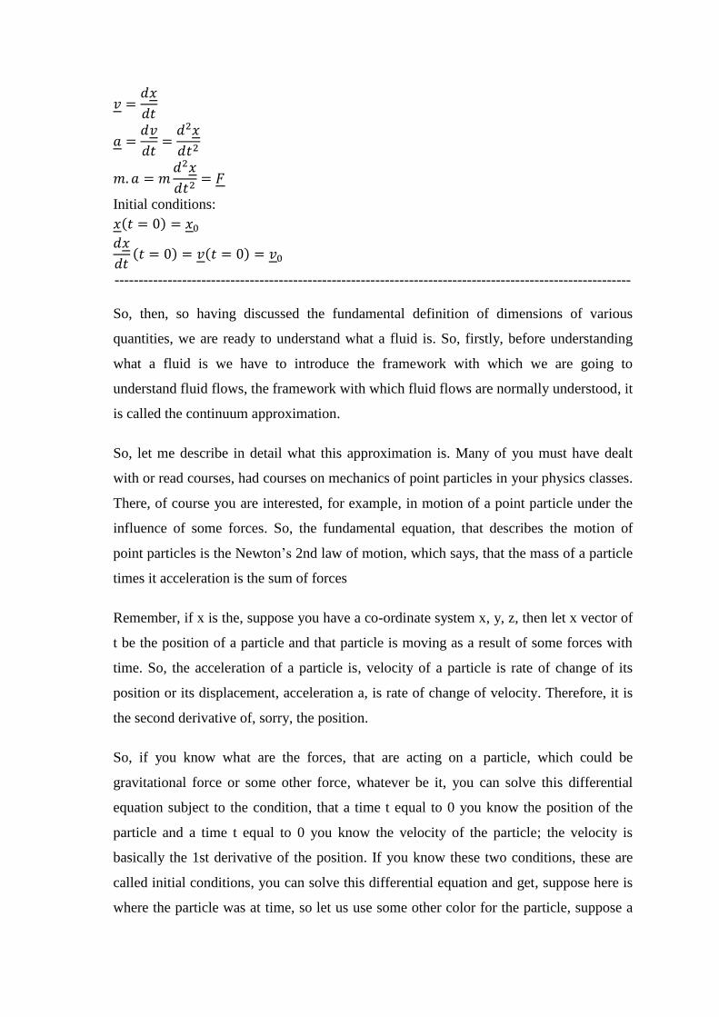
Remember, if x is the, suppose you have a co-ordinate system x, y, z, then let x vector of
t be the position of a particle and that particle is moving as a result of some forces with
time. So, the acceleration of a particle is, velocity of a particle is rate of change of its
position or its displacement, acceleration a, is rate of change of velocity. Therefore, it is
the second derivative of, sorry, the position.
So, if you know what are the forces, that are acting on a particle, which could be
gravitational force or some other force, whatever be it, you can solve this differential
equation subject to the condition, that a time t equal to 0 you know the position of the
particle and a time t equal to 0 you know the velocity of the particle; the velocity is
basically the 1st derivative of the position. If you know these two conditions, these are
called initial conditions, you can solve this differential equation and get, suppose here is
where the particle was at time, so let us use some other color for the particle, suppose a
particle was here at time t equal to 0 and you know what its velocity is by solving this
equation, you can find the, what is called, the trajectory of the particle.
So, sometimes it is simply called particle trajectory. This is simply the positions of the
particle at various time instances as you follow the particle and this is a time t equal to 0;
it is a time t. So, this is the position of the particle at time t. So, this is how one
understands or one tries to understand motion of point particles in Newtonian mechanics.
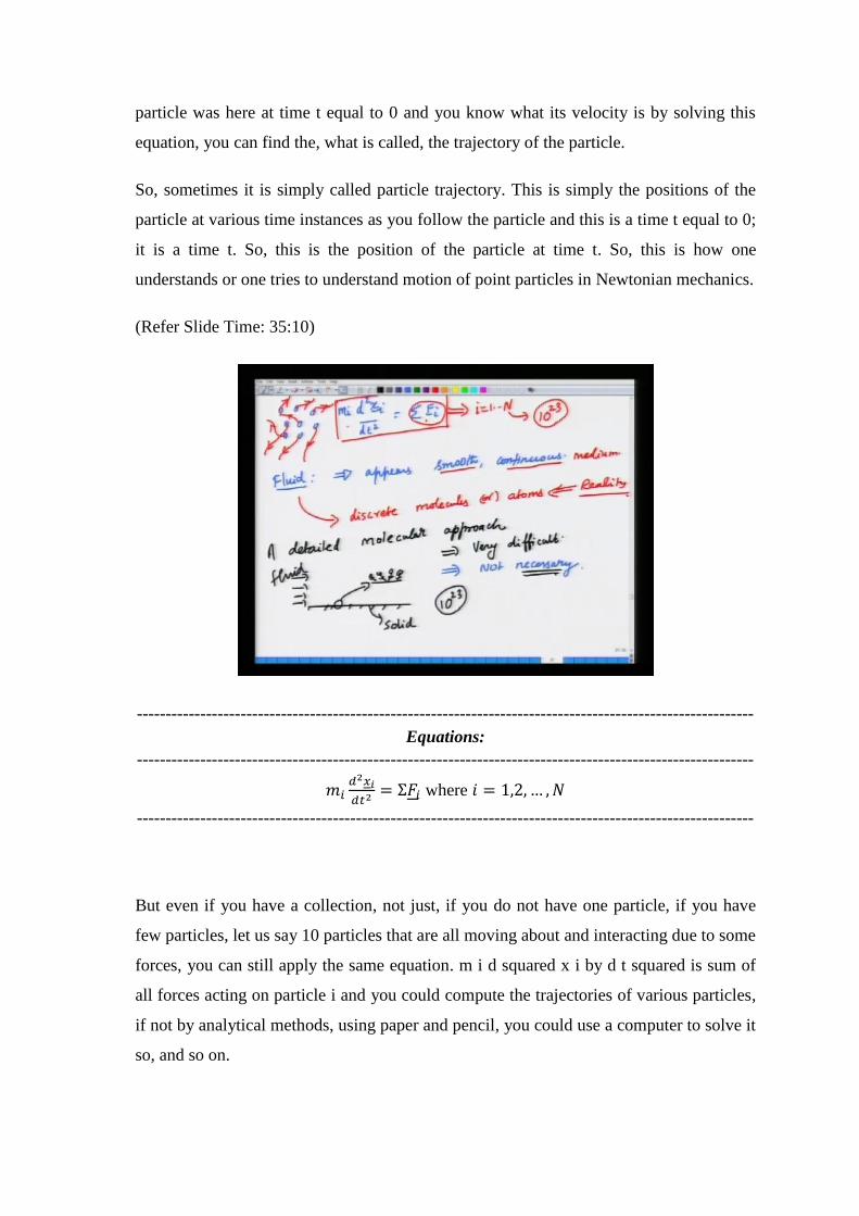
(Refer Slide Time: 35:10)
-----------------------------------------------------------------------------------------------------------
Equations:
-----------------------------------------------------------------------------------------------------------
where
-----------------------------------------------------------------------------------------------------------
But even if you have a collection, not just, if you do not have one particle, if you have
few particles, let us say 10 particles that are all moving about and interacting due to some
forces, you can still apply the same equation. m i d squared x i by d t squared is sum of
all forces acting on particle i and you could compute the trajectories of various particles,
if not by analytical methods, using paper and pencil, you could use a computer to solve it
so, and so on.
So, this is how one does, one understands motion in normal particle mechanics, but if
you consider a fluid, a chunk of fluid, if you take a glass of water or fluid flowing in a
pipe fluid, it appears smooth and continuous towards, you know, unaided senses. For
example, unless you, we use a sophisticated microscope, like an electron microscope or
something, we cannot discern the fact, that a fluid has discrete molecules or atoms
present in it. A fluid, normally, to our naked eyes appears smooth, continuous; it appears
smooth and continuous. But, the ultimate reality is a fluid is comprised of discrete
entities, which could be molecules or atoms. This is a reality, but we do not perceive this
reality using our normal senses. We do see a fluid as the smooth and continuous medium.
Now, as I told you in the beginning, fluid mechanics is concerned with forces, that occur
in flowing fluids for prescribed motion or we are interested in calculating the motion for
prescribed forces. If that is the case, how do we go about calculating forces if the reality
of the fluid is actually discrete and not continuous?
So, a fluid is, complied, comprised of discrete molecules and a whole number of them
and the force is, for example, a solid object, phase, phases because of the forces, that are
exerted fundamentally by all these molecules on the solid surface.
So, while that is the reality it is not really possible for us to find the forces that are
exerted by all these innumerable number of molecules of a fluid on a solid surface. So, a
detailed molecular approach of understanding fluid flow is very, very difficult, that
would amount to solving. For example, if you look at this equation, which is essentially
Newton’s laws for whole bunch of molecules or particles, here the, the number of
particles i goes from 1 to n. If n is a total number of molecules or particles and this n is
of the order of 20, 10 to the 23, Avogadro number of molecules. Even if you consider 1
mole of liquid, like water, there is 10 to the 23 molecules. So, there are huge number of
molecules, which are just, it is not just possible to solve the Newton’s equations even if
we know all the forces accurately, that are acting at a molecular level. So, a detailed
molecular approach or solution to the problem is not easy, it is very, very difficult.
And secondly, I will argue, that it is not necessary to have a detailed molecular approach
to understanding many engineering fluid flow problems. For example, if you are
interested in the force that is experienced by a plate, this is one of the most common
problems in fluid flows. So, you take a rigid plate and fluid is flowing in some fashion
and you are interested in what is the force that is exerted by the fluid on the solid
surface? This is the solid surface; this is the fluid. Ultimately, we will all agree, that if
you take and blow up this region, there are molecules that come and collide and so on
and, and forces are ultimately due to these interactions.
But if you have to collect data for all these 10 to the 23 molecules, that are hitting the
solid, it is just not practically possible to compute the force even if you have a fully
molecular detailed approach or detailed data or information available with you. It is not
feasible to compute forces using such large number of data. So, it is just not possible, so
it is just not.
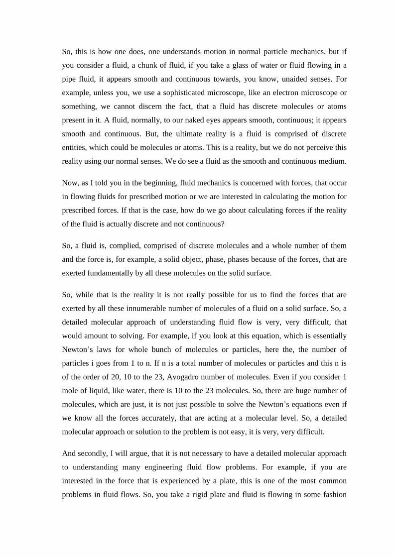
(Refer Slide Time: 40:20)
And so, even if you have a detailed molecular picture it is not necessary, as I will show
in the next slide, because ultimately, what we have measured using devices, we measure
only averages, specifically we measure time averages.
Even if you consider at a molecular level, a whole lot of molecules, that are coming and
hitting a solid surface and that results in the force. No macroscopic measuring device
will measure or resolve, the force is exerted by individual molecules. Instead, we are
going to measure only averages of various quantities. So, this again goes to reinforce
notion, that a detailed molecular picture or detailed molecular approach is not necessary
from the context of understanding what is the force exerted by a fluid on a solid surface
because that is simply not necessary.
So, what the continuum, I first, I will first state what the continuum approximation
means and then, I am going to justify when continuum approximation works and finally,
I will also point out context where the continuum approximation may fail. So, what is the
continuum hypothesis? The continuum hypothesis assumes the fluid to be a smooth,
continuous medium. And various quantities of the fluid, various properties of the fluid
for example, density, which is denoted by the letter rho and pressure, pressure is nothing,
but the force, that is exerted by the fluid per area of any surface. And velocity of the
fluid, velocity is normally denoted by the vector v, velocity is a quantity, is a vectorial
quantity, it has both magnitude and direction.
So, we will in this course, the notation for vector, vectors will be denoted by an
underscore. So, v underscore means it is a vector.
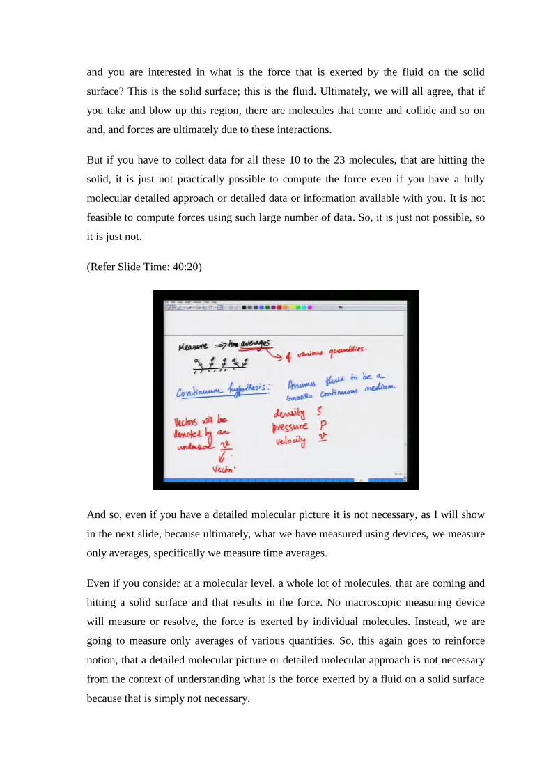
(Refer Slide Time: 43:07)
So, there are various quantities in a fluid, so the various quantities in a fluid, like density,
pressure, velocity, all these are assumed to be smooth functions of spatial coordinates.
For example, x, y, z because you want to analyze the flow with respect to a coordinate
system, the simplest is a rectangular coordinate or Cartesian coordinate, where you have
three mutually perpendicular axes. So, all these quantities, density, pressure, velocity are
assumed or postulated to be smooth functions of x, y, z and time t.
So, this is the essential statement of continuum hypothesis, that at each and every point
in the fluid, each and every point in the, with respect to the coordinate system, we can
ascribe properties such as density, velocity, pressure temperature unique values and these
are functions, which are smoothly varying with space and time.
Now, I am going to illustrate why this hypothesis is powerful and that will also point us
to the special cases where this hypothesis may fail.
(Refer Slide Time: 44:20)
-----------------------------------------------------------------------------------------------------------
Equations:
-----------------------------------------------------------------------------------------------------------
-----------------------------------------------------------------------------------------------------------
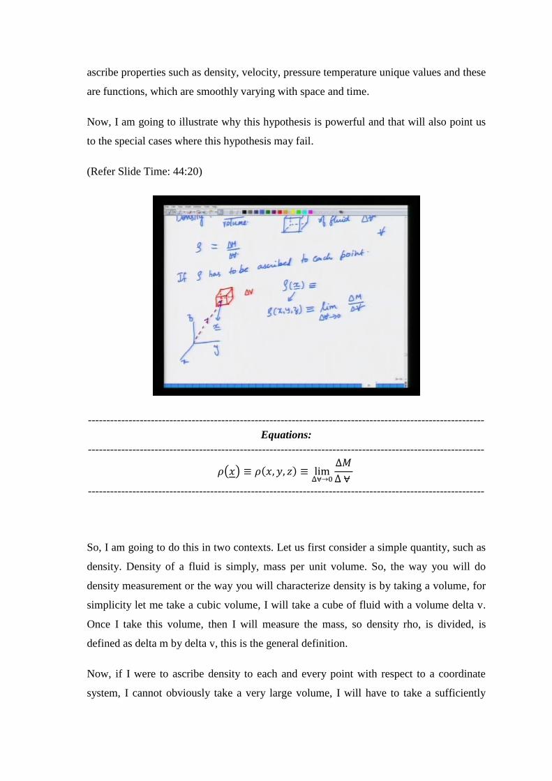
So, I am going to do this in two contexts. Let us first consider a simple quantity, such as
density. Density of a fluid is simply, mass per unit volume. So, the way you will do
density measurement or the way you will characterize density is by taking a volume, for
simplicity let me take a cubic volume, I will take a cube of fluid with a volume delta v.
Once I take this volume, then I will measure the mass, so density rho, is divided, is
defined as delta m by delta v, this is the general definition.
Now, if I were to ascribe density to each and every point with respect to a coordinate
system, I cannot obviously take a very large volume, I will have to take a sufficiently
small volume. So, if I were to, if density has to be ascribed to each point in a fluid flow,
then what I would do is I would take a point and around that point I will construct a
cubic volume element of volume delta v and I will define density at that point x. x vector
is defined as rho, this is a short form for rho, as a function of x, y, z.
So, I will denote a point with this by labeling it with its position vector, x is defined as
limit density around, suppose this point is denoted by x with respect to a coordinate
system. So, let us say this is the point x, this is the position vector of the point x, then
density is defined as, the fundamental definition of density is limit delta v. As I shrink
that volume to that point, I will measure, sorry, we erase this and I will keep this, so limit
delta v going to 0 delta m.
So, just to differentiate, since the symbol v is used for both velocity and volume, I am
going to, as far as possible, denote volumes with the v cross because this will remove the
confusion between volume and velocity because we, we use v the symbol capital V for
velocity and small v for, sorry, capital V for volume and small v for velocity, so I will
use v cross delta m by delta v. This is mass per unit volume as you shrink the volume to
a point.
Now, then the next question comes, when can we naturally shrink the volume to a point?
Can we shrink that volume arbitrarily to a point? Well, you cannot naturally shrink this
volume to 0 because you need some finite volume to get some finite mass. So, we have
to be a little careful in doing this.
(Refer Slide Time: 47:50)
-----------------------------------------------------------------------------------------------------------
Equations:
-----------------------------------------------------------------------------------------------------------
where is dia of a molecule
For at a point:
-----------------------------------------------------------------------------------------------------------
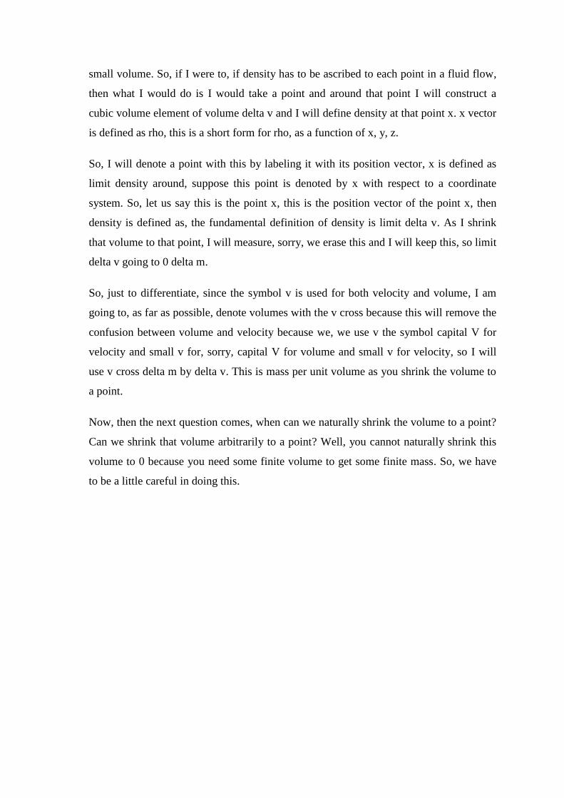
So, let us consider what I am going to, let us do a thought experiment, wherein we are
going to measure the density as limit delta v going to 0 delta m by delta v. As a function,
let us say, since we are going to span a wide ranges of volumes I am going to plot it as a
function of logarithm of the volume. I am going to plot in a hypothetical thought
experiment where you measure density of a fluid by varying the size of the probe
volume, the cubic volume, that I drew in the last slide. So, how will this look?
Now, if your volume is very, very small, if delta v, suppose delta v is L cube, delta v is
the volume of a cube of length or side L. If L is comparable to molecular dimensions, let
us say you consider a fluid, a liquid, the diameter of this liquid molecules, let us say a, if
L is comparable to a, then if you take a tiny volume that is comparable to a cube. If then
at a, this volume is comparable to molecular dimensions, dimensions of molecular
volume, at a molecular level.
You know, that even in a, from basic physical chemistry or physics we will know, that
molecules are undergoing very, very violent and strong thermal motion. So, it is very, it
is a very, very probabilistic thing to find a volume, is to find a molecule of diameter a in
a volume of diameter roughly a cube proportional to a cube because these molecules will
be undergoing very, very strong thermal motion.
So, when your volume is very, very small, your density will highly fluctuate with respect
to given spatial point because at given spatial point may either have a molecule or not
and even if this has two molecules, the number of molecules will fluctuate wildly. So,
initially what you will find, when, when the volume is very, very small, you will find,
that the density fluctuates a lot, but eventually we will find, that the density settles down.
Now, typically, this is about of the order of 10 to the minus 9 millimeter cube, that is,
when your size of the cube is of the order of 1 micron, the density would have nicely
settled down to a flat value, a constant value and from this point on, regardless of how
you choose the volume to be, the value of the density that you will get will remain the
same. So, this is the continuum value of density.
So, this is what we mean by density at a point because in these huge ranges of volume,
the density is a well defined quantity. Now, eventually, if you keep increasing the size of
the cube, you will start seeing density differences that are due to genuine macroscopic
variations in density. So, clearly, you cannot take this as a point value.
So, if the size of the cube in which you are using, which you are probing the density or
measuring the density, if the size of the cube is large compared to molecular dimensions,
a is the diameter of a molecule for example, and it is small compared to the system
dimension for example, it could be the diameter of a pipe in which the fluid is flowing
for example, or the diameter of a tank in which the fluid is present, then the density at a
point makes sense. And even if you change the, the probe volume, you will find a unique
value, that is ascribed to the density at a point and you can repeat this for different points
in a fluid. And therefore, this is remember, density as a function of this probe volume.
(Refer Slide Time: 52:04)
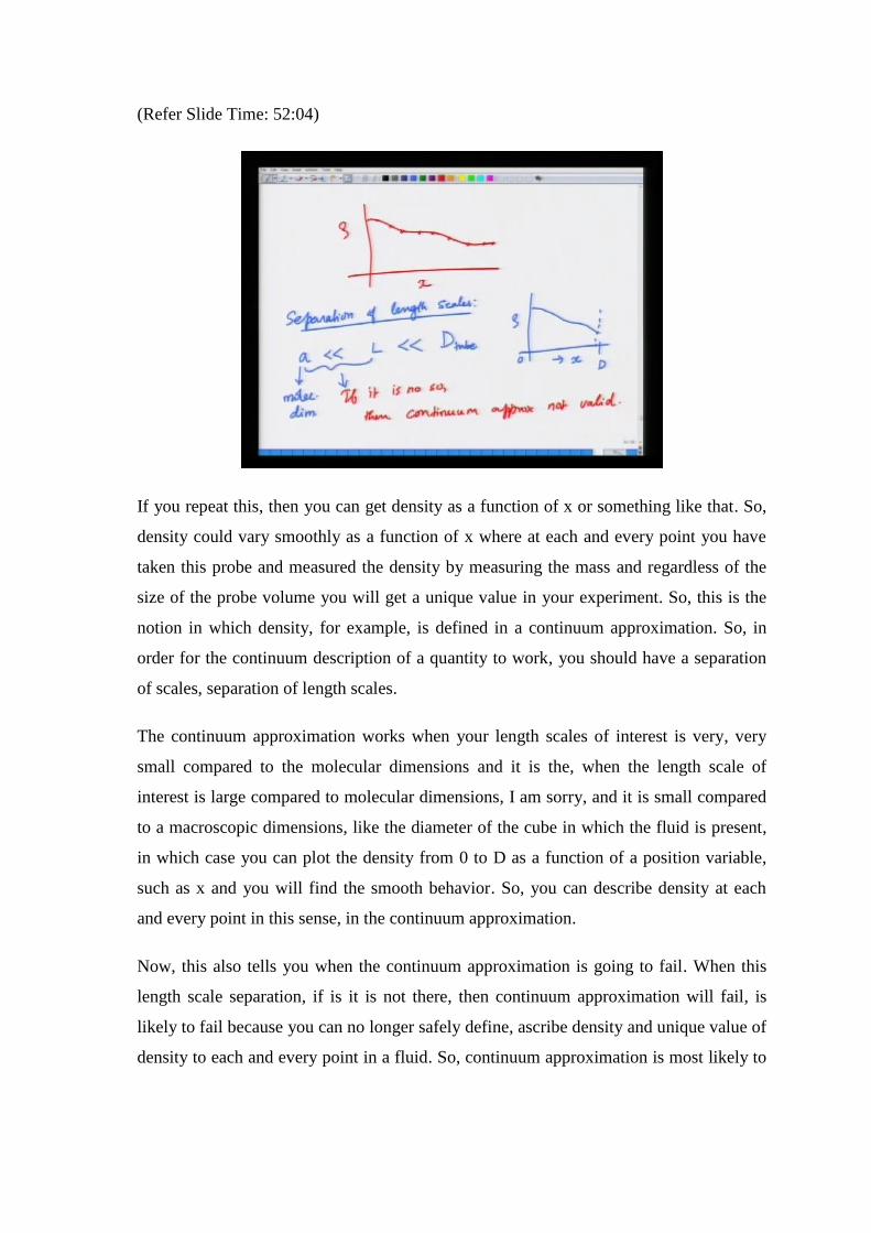
If you repeat this, then you can get density as a function of x or something like that. So,
density could vary smoothly as a function of x where at each and every point you have
taken this probe and measured the density by measuring the mass and regardless of the
size of the probe volume you will get a unique value in your experiment. So, this is the
notion in which density, for example, is defined in a continuum approximation. So, in
order for the continuum description of a quantity to work, you should have a separation
of scales, separation of length scales.
The continuum approximation works when your length scales of interest is very, very
small compared to the molecular dimensions and it is the, when the length scale of
interest is large compared to molecular dimensions, I am sorry, and it is small compared
to a macroscopic dimensions, like the diameter of the cube in which the fluid is present,
in which case you can plot the density from 0 to D as a function of a position variable,
such as x and you will find the smooth behavior. So, you can describe density at each
and every point in this sense, in the continuum approximation.
Now, this also tells you when the continuum approximation is going to fail. When this
length scale separation, if is it is not there, then continuum approximation will fail, is
likely to fail because you can no longer safely define, ascribe density and unique value of
density to each and every point in a fluid. So, continuum approximation is most likely to

be not valid. Now, the same thing can be extended to quantities, like pressure for
example.
(Refer Slide Time: 54:08)
-----------------------------------------------------------------------------------------------------------
Equations:
-----------------------------------------------------------------------------------------------------------
-----------------------------------------------------------------------------------------------------------
Let us take the case of pressure where you take a rectangular surface and this is a solid
surface a flat surface and which, let us say, that are fluid molecules, gas molecules, that
are coming and colliding and bouncing back, and so on. So, the pressure is
fundamentally defined as the normal force per unit area of the solid. By a normal force I
mean the force that is perpendicular to the plain of the solid. If n is the unit normal to the
solid, it is the force that is exerted by the fluid. So, if you have a fluid, the force exerted
by the fluid on the solid in the direction of the normal to the solid per area of the solid.
So, this is the fundamental definition of pressure.
But why does pressure happen at a molecular level? It happens because of molecular
collisions. Whenever molecules come and collide, the rate of change of momentum of
these molecules appears as a force on the surface and that force per unit area is a
pressure. So, the pressure is fundamentally defined as limit as delta a goes to 0 delta F by
delta A.
So, the continuum hypothesis says, that it is not necessary to worry about individual
molecules. The force is exerted by individual molecules because they are too huge in
number. So, it is all and any macroscopic probing device will measure only averages. So,
even if you consider a very, very tiny area of the order of 1 micron by 1 micron, one can
use simple kinetic theory, that one’s read in physical chemistry. So, this area is 10 to the
minus 12 meter squared. It is very, very small, but the number of molecular collisions is
huge.
If you consider air at room temperature that collide per unit time per second, is from
kinetic theory of gases, that one reads in physical chemistry, is of the order of 10 to the 7
molecules per second. So, it is a huge number. So, even within a second, any probing
device will not measure individual collisions. So, devices will measure only averages.
We will stop here and we will continue from the next lecture.
Recommended