first a digression The POC
Ranking the MethodsJennie Watson-Lamprey
October 29, 2007

A Digression
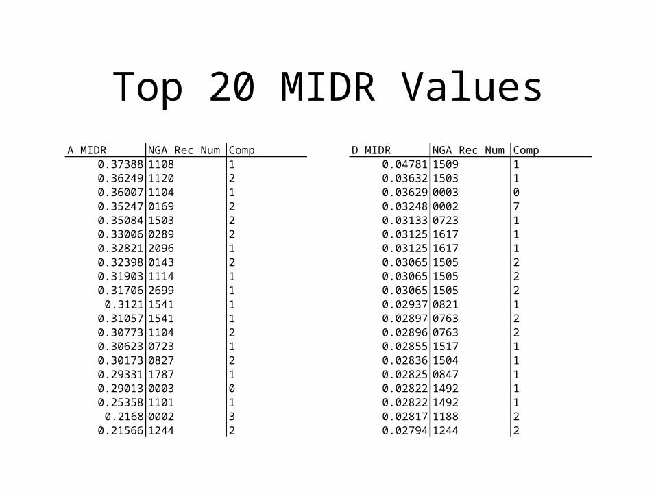
Top 20 MIDR ValuesD MIDR NGA Rec Num Comp
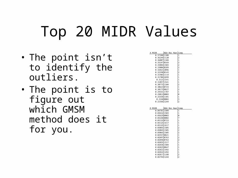
0.04781 1509 10.03632 1503 10.03629 0003 00.03248 0002 70.03133 0723 10.03125 1617 10.03125 1617 10.03065 1505 20.03065 1505 20.03065 1505 20.02937 0821 10.02897 0763 20.02896 0763 20.02855 1517 10.02836 1504 10.02825 0847 10.02822 1492 10.02822 1492 10.02817 1188 20.02794 1244 2
A MIDR NGA Rec Num Comp0.37388 1108 10.36249 1120 20.36007 1104 10.35247 0169 20.35084 1503 20.33006 0289 20.32821 2096 10.32398 0143 20.31903 1114 10.31706 2699 1
0.3121 1541 10.31057 1541 10.30773 1104 20.30623 0723 10.30173 0827 20.29331 1787 10.29013 0003 00.25358 1101 1
0.2168 0002 30.21566 1244 2
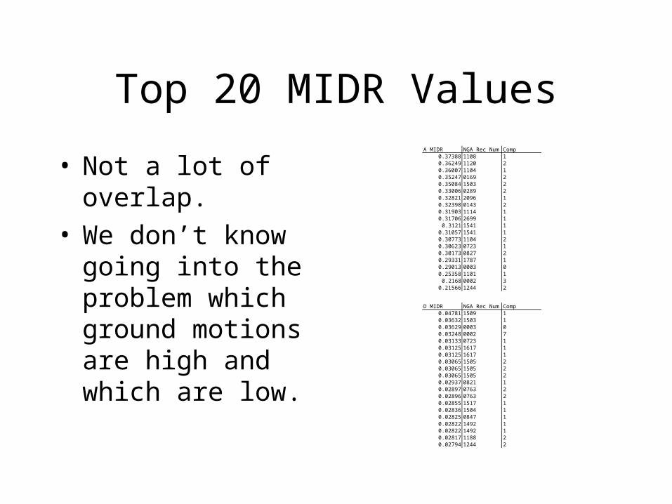
Top 20 MIDR Values
D MIDR NGA Rec Num Comp0.04781 1509 10.03632 1503 10.03629 0003 00.03248 0002 70.03133 0723 10.03125 1617 10.03125 1617 10.03065 1505 20.03065 1505 20.03065 1505 20.02937 0821 10.02897 0763 20.02896 0763 20.02855 1517 10.02836 1504 10.02825 0847 10.02822 1492 10.02822 1492 10.02817 1188 20.02794 1244 2
• Not a lot of overlap.• We don’t know
going into the problem which ground motions are high and which are low.
A MIDR NGA Rec Num Comp0.37388 1108 10.36249 1120 20.36007 1104 10.35247 0169 20.35084 1503 20.33006 0289 20.32821 2096 10.32398 0143 20.31903 1114 10.31706 2699 1
0.3121 1541 10.31057 1541 10.30773 1104 20.30623 0723 10.30173 0827 20.29331 1787 10.29013 0003 00.25358 1101 1
0.2168 0002 30.21566 1244 2
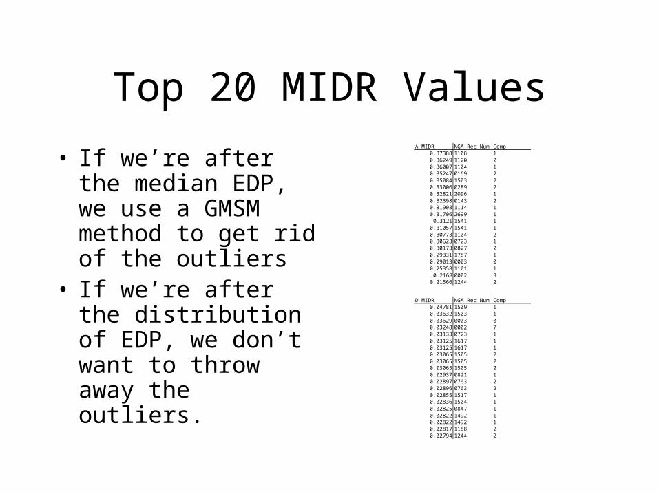
Top 20 MIDR Values
D MIDR NGA Rec Num Comp0.04781 1509 10.03632 1503 10.03629 0003 00.03248 0002 70.03133 0723 10.03125 1617 10.03125 1617 10.03065 1505 20.03065 1505 20.03065 1505 20.02937 0821 10.02897 0763 20.02896 0763 20.02855 1517 10.02836 1504 10.02825 0847 10.02822 1492 10.02822 1492 10.02817 1188 20.02794 1244 2
• If we’re after the median EDP, we use a GMSM method to get rid of the outliers
• If we’re after the distribution of EDP, we don’t want to throw away the outliers.
A MIDR NGA Rec Num Comp0.37388 1108 10.36249 1120 20.36007 1104 10.35247 0169 20.35084 1503 20.33006 0289 20.32821 2096 10.32398 0143 20.31903 1114 10.31706 2699 1
0.3121 1541 10.31057 1541 10.30773 1104 20.30623 0723 10.30173 0827 20.29331 1787 10.29013 0003 00.25358 1101 1
0.2168 0002 30.21566 1244 2
Top 20 MIDR Values
D MIDR NGA Rec Num Comp0.04781 1509 10.03632 1503 10.03629 0003 00.03248 0002 70.03133 0723 10.03125 1617 10.03125 1617 10.03065 1505 20.03065 1505 20.03065 1505 20.02937 0821 10.02897 0763 20.02896 0763 20.02855 1517 10.02836 1504 10.02825 0847 10.02822 1492 10.02822 1492 10.02817 1188 20.02794 1244 2
• The point isn’t to identify the outliers.
• The point is to figure out which GMSM method does it for you.
A MIDR NGA Rec Num Comp0.37388 1108 10.36249 1120 20.36007 1104 10.35247 0169 20.35084 1503 20.33006 0289 20.32821 2096 10.32398 0143 20.31903 1114 10.31706 2699 1
0.3121 1541 10.31057 1541 10.30773 1104 20.30623 0723 10.30173 0827 20.29331 1787 10.29013 0003 00.25358 1101 1
0.2168 0002 30.21566 1244 2

The POC
Calculating the Point of Comparison
• Time series from a bin of M, R – Should work for a median– Too much variability!
• Time series from a bin of M, R corrected for the difference between the recorded event and the design event– Not enough records to push the structure into the nonlinear
range -> not a good estimator of rare response values
Calculating the Point of Comparison
• Current Method:– Run scaled and unscaled time series through a structural
model– Perform a regression on a response parameter using time
series properties (spectral acceleration)– Use predictive equations to define the joint distribution of the
time series properties– Integrate the regression over the joint distribution– This gives a distribution of a response parameter
Method for Estimating Point of Comparison
1. A suite of records from Mw6.75-7.25, Rrup 0-20km events was developed. A total of 98 records were distributed to the group June 26th.
2. The suite is run through each model using scale factors of 1, 2, 4 and 8.
3. A model of the desired structural response parameter using properties of the input time series (e.g. Sa(T1), Sa(2T1), duration, etc.) is developed.
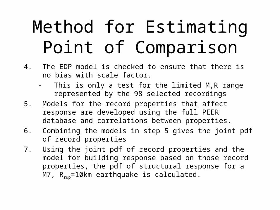
Method for Estimating Point of Comparison
4. The EDP model is checked to ensure that there is no bias with scale factor.
- This is only a test for the limited M,R range represented by the 98 selected recordings
5. Models for the record properties that affect response are developed using the full PEER database and correlations between properties.
6. Combining the models in step 5 gives the joint pdf of record properties
7. Using the joint pdf of record properties and the model for building response based on those record properties, the pdf of structural response for a M7, Rrup=10km earthquake is calculated.
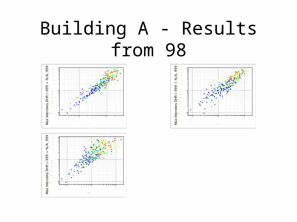
Building A - Results from 98
0.001
0.01
0.007
0.005
0.003
0.002
0.1
0.07
0.05
0.03
0.02
Max Interstory Drift (-999 = N/A, 999 = 0)
.1 .07 .04 .02
1 .7 .5 .3 .2 2 3 4
1s
0.001
0.01
0.007
0.005
0.003
0.002
0.1
0.07
0.05
0.03
0.02
Max Interstory Drift (-999 = N/A, 999 = 0)
.01 .1 .06 .03
1 .7 .5 .3 .2 2
2s
0.001
0.01
0.007
0.005
0.003
0.002
0.1
0.07
0.05
0.03
0.02
Max Interstory Drift (-999 = N/A, 999 = 0)
.1 .06
1 .7 .4 .2
10 7 5 3 2 20
0.4s
Building A - Regression
€
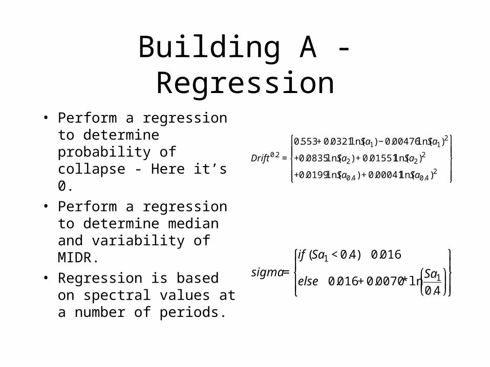
Drift0.2 =
0.553+ 0.0321ln(Sa1) − 0.00476ln(Sa1)2
+0.0835ln(Sa2) + 0.01551ln(Sa2)2
+0.0199ln(Sa0.4 ) + 0.00041ln(Sa0.4 )2
⎧
⎨ ⎪ ⎪
⎩ ⎪ ⎪
⎫
⎬ ⎪ ⎪
⎭ ⎪ ⎪
€
sigma =
if (Sa1 < 0.4) 0.016
else 0.016 + 0.0070* lnSa1
0.4
⎛
⎝ ⎜
⎞
⎠ ⎟
⎧
⎨ ⎪
⎩ ⎪
⎫
⎬ ⎪
⎭ ⎪
• Perform a regression to determine probability of collapse - Here it’s 0.
• Perform a regression to determine median and variability of MIDR.
• Regression is based on spectral values at a number of periods.
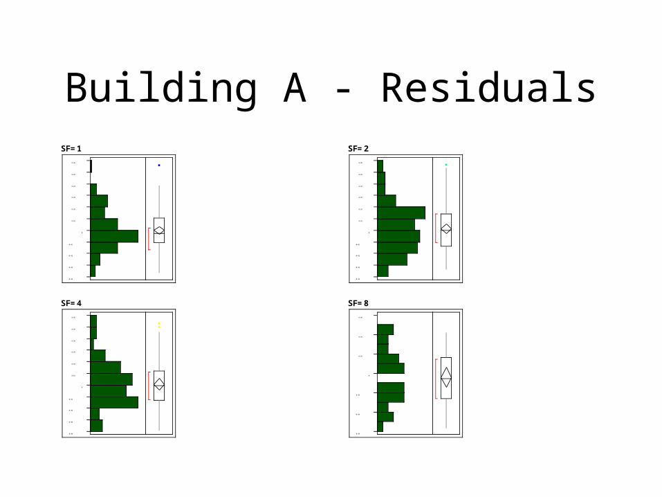
Building A - Residuals
SF=8
-0.06
-0.04
-0.02
0
0.02
0.04
0.06
SF=4
-0.04
-0.03
-0.02
-0.01
0
0.01
0.02
0.03
0.04
0.05
0.06
SF=1
-0.04
-0.03
-0.02
-0.01
0
0.01
0.02
0.03
0.04
0.05
0.06
SF=2
-0.04
-0.03
-0.02
-0.01
0
0.01
0.02
0.03
0.04
0.05
0.06

Building A - Integration
€
P(MIDR > z | M ,R,Sa1)= fε (ε Sa0.4) fε (ε Sa2
)P MIDR > Z | Sa1,Sa0.4 ,Sa2( ) dε Sa0.4dε Sa2
ε Sa0.4
∫ε Sa2
∫

Building A - Integration
€
Sa2 = exp ln Sa2med(M ,R)+ c1ε Sa0.4σ Sa2
+ c2ε Sa1σ Sa2
+ 1− c12 1− c2
2σ Sa2ε Sa2( )
€
Sa0.4 = exp ln Sa0.4med(M ,R)+ b1ε Sa1σ Sa0.4
+ 1− b12σ Sa0.4
ε Sa0.4( )

Building A - Integration Really
QuickTime™ and aTIFF (LZW) decompressor
are needed to see this picture.
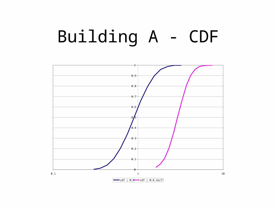
Building A - CDF
0
0.1
0.2
0.3
0.4
0.5
0.6
0.7
0.8
0.9
1
0.1 1 10
cdf | M,R cdf | M,R,Sa(T1)
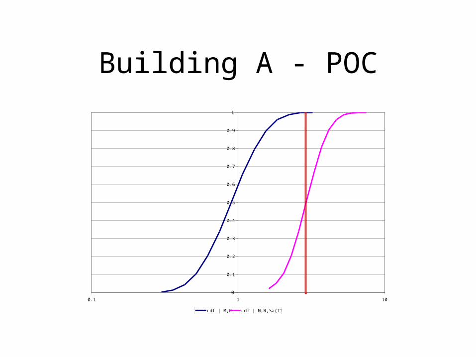
Building A - POC
0
0.1
0.2
0.3
0.4
0.5
0.6
0.7
0.8
0.9
1
0.1 1 10
cdf | M,R cdf | M,R,Sa(T1)

POC Questions?

Ranking the Methods
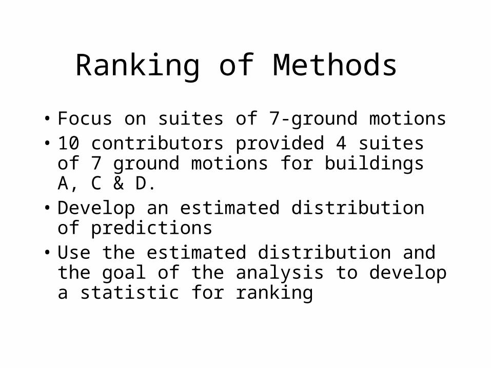
Ranking of Methods
• Focus on suites of 7-ground motions• 10 contributors provided 4 suites of 7
ground motions for buildings A, C & D.• Develop an estimated distribution of
predictions• Use the estimated distribution and the
goal of the analysis to develop a statistic for ranking
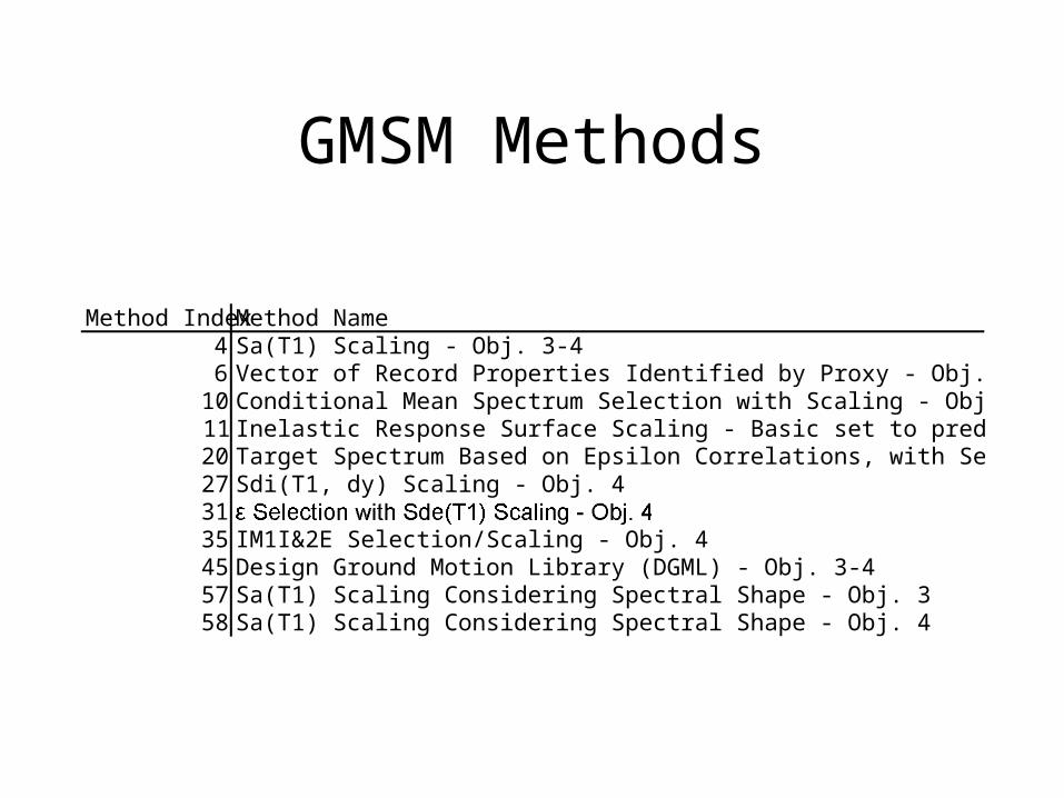
GMSM Methods
Method Index Method Name4 Sa(T1) Scaling - Obj. 3-46 Vector of Record Properties Identified by Proxy - Obj. 4
10 Conditional Mean Spectrum Selection with Scaling - Obj. 411 Inelastic Response Surface Scaling - Basic set to predict Obj. 420 Target Spectrum Based on Epsilon Correlations, with Selection based on M, R, Directivity and Epsilon (refine this name)27 Sdi(T1, dy) Scaling - Obj. 43135 IM1I&2E Selection/Scaling - Obj. 445 Design Ground Motion Library (DGML) - Obj. 3-457 Sa(T1) Scaling Considering Spectral Shape - Obj. 358 Sa(T1) Scaling Considering Spectral Shape - Obj. 4
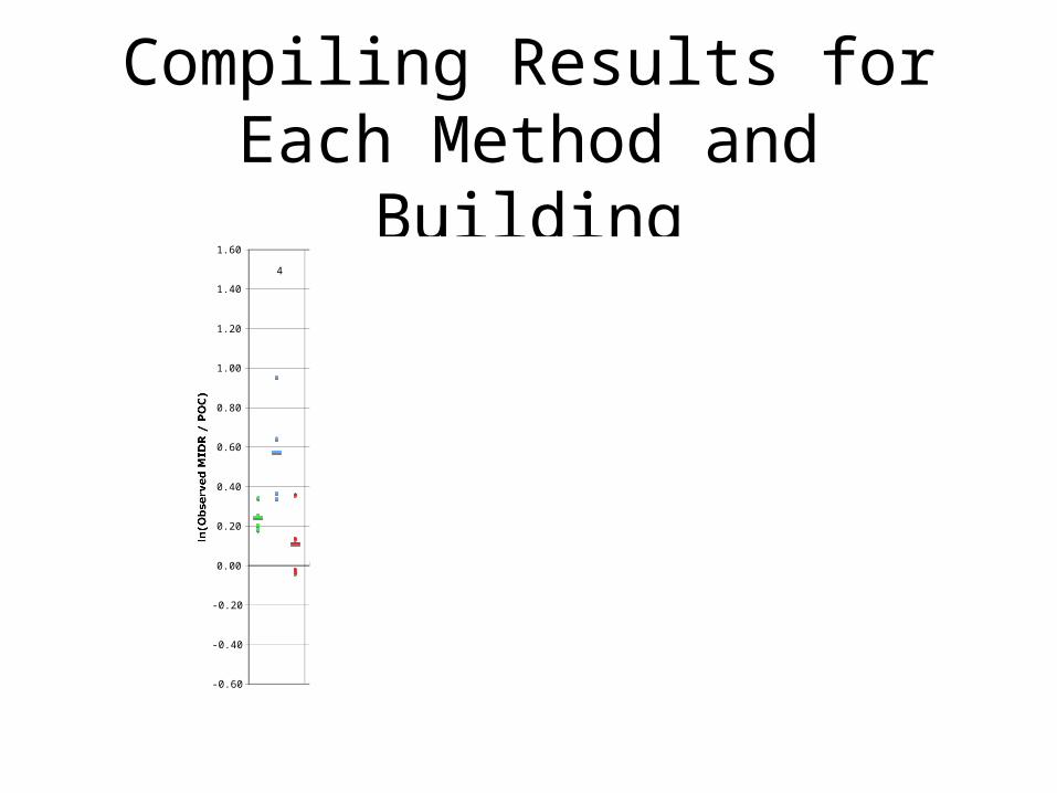
Compiling Results for Each Method and Building
-0.60
-0.40
-0.20
0.00
0.20
0.40
0.60
0.80
1.00
1.20
1.40
1.60
ln(Observed MIDR / POC)
4 6 10 11 20 27 31 35 45 57 58
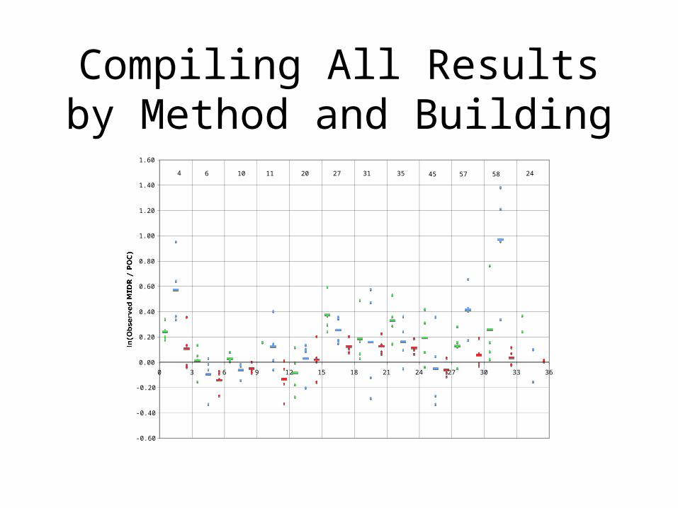
Compiling All Results by Method and Building
-0.60
-0.40
-0.20
0.00
0.20
0.40
0.60
0.80
1.00
1.20
1.40
1.60
0 3 6 9 12 15 18 21 24 27 30 33 36
ln(Observed MIDR / POC)
4 6 10 11 20 27 31 35 45 57 58 24
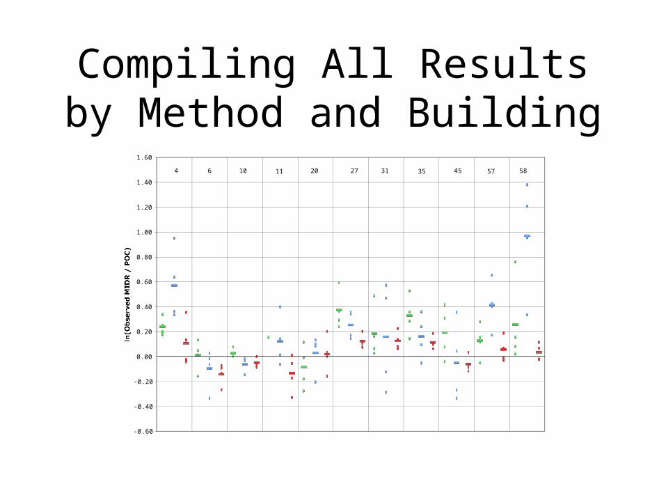
Compiling All Results by Method and Building
-0.60
-0.40
-0.20
0.00
0.20
0.40
0.60
0.80
1.00
1.20
1.40
1.60
ln(Observed MIDR / POC)
4 6 10 11 20 27 31 35 45 57 58
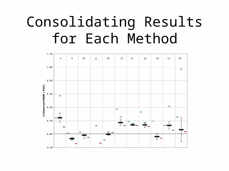
Consolidating Results for Each Method
-0.20
0.00
0.20
0.40
0.60
0.80
1.00
1.20
ln(Observed MIDR / POC)
4 6 10 11 20 27 31 35 45 57 58
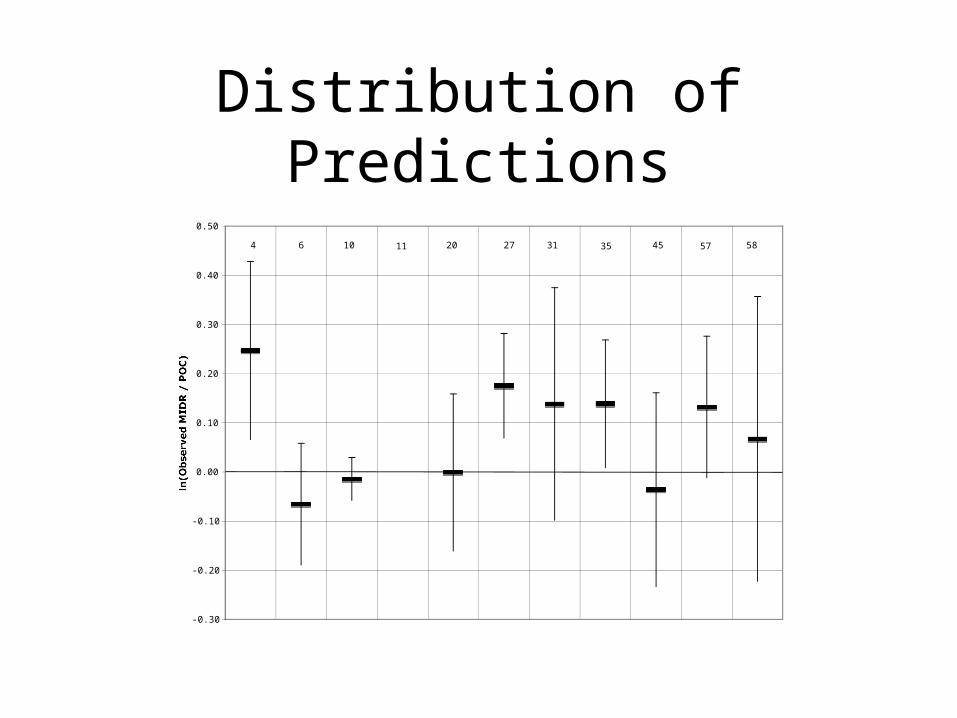
Distribution of Predictions
-0.30
-0.20
-0.10
0.00
0.10
0.20
0.30
0.40
0.50
ln(Observed MIDR / POC)
4 6 10 11 20 27 31 35 45 57 58
Ranking Statistic
• Goal: Accurate estimate of MIDR | M, R, Sa
• Statistic: P ( -0.1 < X < 0.1)
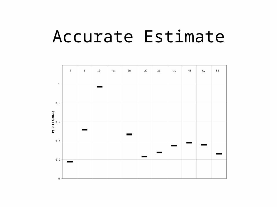
Accurate Estimate
0
0.2
0.4
0.6
0.8
1
1.2
P(-0.1<X<0.1)
4 6 10 11 20 27 31 35 45 57 58
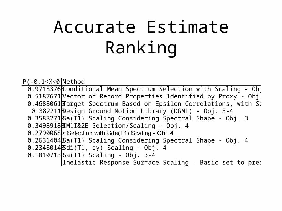
Accurate Estimate Ranking
P(-0.1<X<0.1) Method0.97183763 Conditional Mean Spectrum Selection with Scaling - Obj. 40.51876716 Vector of Record Properties Identified by Proxy - Obj. 40.46880619 Target Spectrum Based on Epsilon Correlations, with Selection based on M, R, Directivity and Epsilon (refine this name)
0.3822118 Design Ground Motion Library (DGML) - Obj. 3-40.35882719 Sa(T1) Scaling Considering Spectral Shape - Obj. 30.34989183 IM1I&2E Selection/Scaling - Obj. 40.279006850.26314043 Sa(T1) Scaling Considering Spectral Shape - Obj. 40.23480143 Sdi(T1, dy) Scaling - Obj. 40.18107139 Sa(T1) Scaling - Obj. 3-4
Inelastic Response Surface Scaling - Basic set to predict Obj. 4
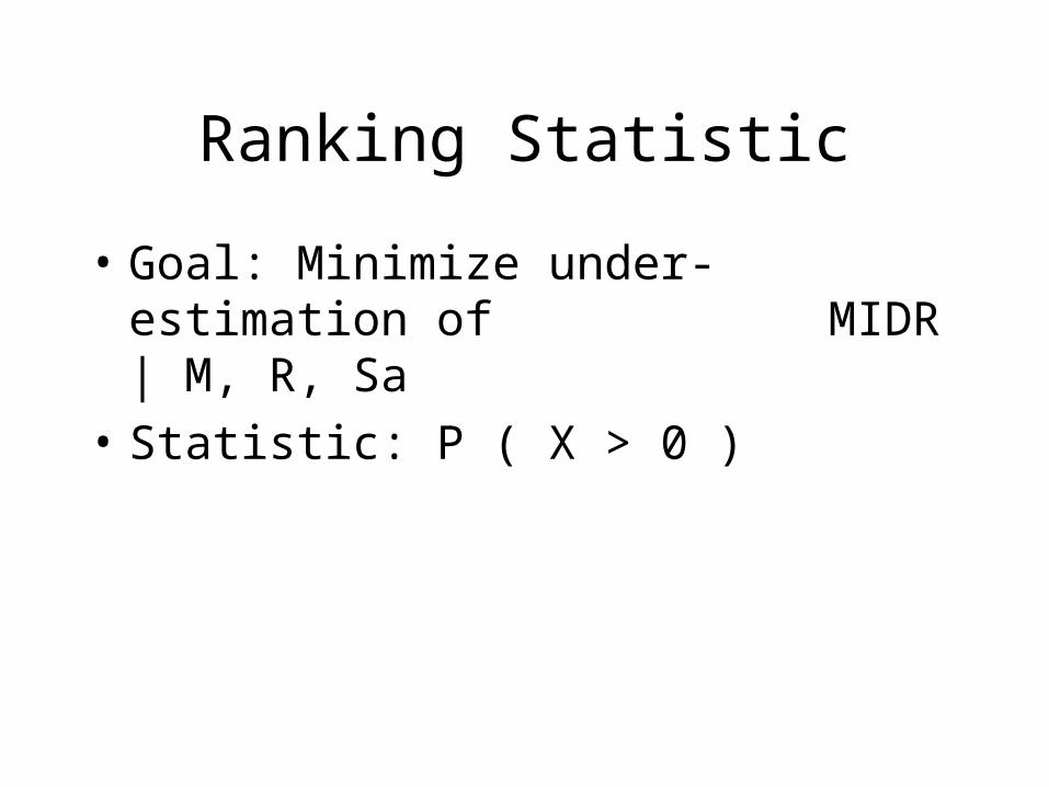
Ranking Statistic
• Goal: Minimize under-estimation of MIDR | M, R, Sa
• Statistic: P ( X > 0 )
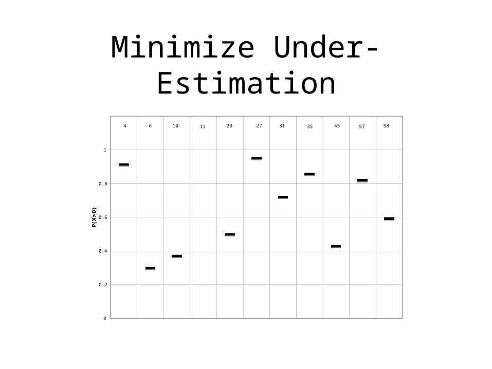
Minimize Under-Estimation
0
0.2
0.4
0.6
0.8
1
1.2
P(X>0)
4 6 10 11 20 27 31 35 45 57 58
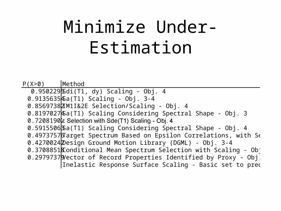
Minimize Under-Estimation
P(X>0) Method0.9502295 Sdi(T1, dy) Scaling - Obj. 4
0.91356354 Sa(T1) Scaling - Obj. 3-40.85697382 IM1I&2E Selection/Scaling - Obj. 40.81970274 Sa(T1) Scaling Considering Spectral Shape - Obj. 30.720819020.59155063 Sa(T1) Scaling Considering Spectral Shape - Obj. 40.49737576 Target Spectrum Based on Epsilon Correlations, with Selection based on M, R, Directivity and Epsilon (refine this name)0.42700242 Design Ground Motion Library (DGML) - Obj. 3-40.37088518 Conditional Mean Spectrum Selection with Scaling - Obj. 40.29797379 Vector of Record Properties Identified by Proxy - Obj. 4
Inelastic Response Surface Scaling - Basic set to predict Obj. 4

Ranking of Methods
• Ranking is dependent on analysis goal.
P(-0.1<X<0.1) Method0.97183763 Conditional Mean Spectrum Selection with Scaling - Obj. 40.51876716 Vector of Record Properties Identified by Proxy - Obj. 40.46880619 Target Spectrum Based on Epsilon Correlations, with Selection based on M, R, Directivity and Epsilon (refine this name)
0.3822118 Design Ground Motion Library (DGML) - Obj. 3-40.35882719 Sa(T1) Scaling Considering Spectral Shape - Obj. 30.34989183 IM1I&2E Selection/Scaling - Obj. 40.279006850.26314043 Sa(T1) Scaling Considering Spectral Shape - Obj. 40.23480143 Sdi(T1, dy) Scaling - Obj. 40.18107139 Sa(T1) Scaling - Obj. 3-4
Inelastic Response Surface Scaling - Basic set to predict Obj. 4
P(X>0) Method0.9502295 Sdi(T1, dy) Scaling - Obj. 4
0.91356354 Sa(T1) Scaling - Obj. 3-40.85697382 IM1I&2E Selection/Scaling - Obj. 40.81970274 Sa(T1) Scaling Considering Spectral Shape - Obj. 30.720819020.59155063 Sa(T1) Scaling Considering Spectral Shape - Obj. 40.49737576 Target Spectrum Based on Epsilon Correlations, with Selection based on M, R, Directivity and Epsilon (refine this name)0.42700242 Design Ground Motion Library (DGML) - Obj. 3-40.37088518 Conditional Mean Spectrum Selection with Scaling - Obj. 40.29797379 Vector of Record Properties Identified by Proxy - Obj. 4
Inelastic Response Surface Scaling - Basic set to predict Obj. 4


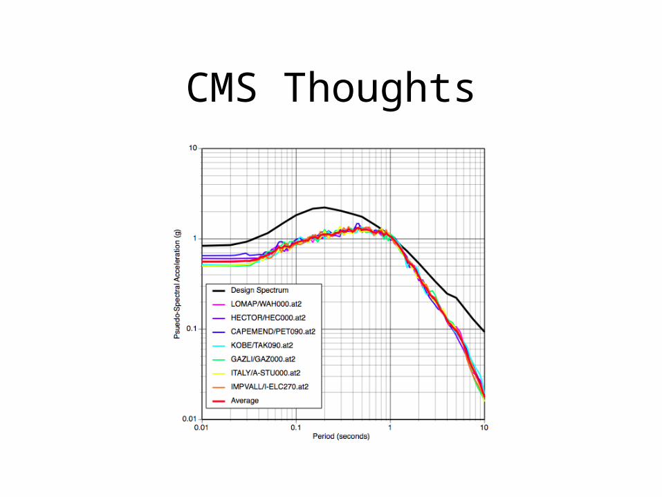
CMS Thoughts
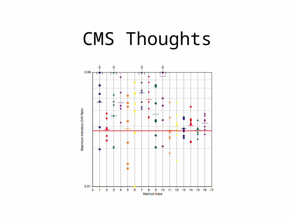
CMS Thoughts
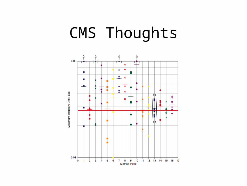
CMS Thoughts

Recommended