FINITE VOLUME ELEMENT METHODS FOR
INCOMPRESSIBLE MISCIBLE DISPLACEMENT
PROBLEMS IN POROUS MEDIA
Thesis
Submitted in partial fulfillment of the requirements
For the degree of
Doctor of Philosophy
by
Sarvesh Kumar
(02409005)
Under the Supervision of
Supervisor: Professor Neela Nataraj
Co-supervisor: Professor Amiya K. Pani
DEPARTMENT OF MATHEMATICS
INDIAN INSTITUTE OF TECHNOLOGY, BOMBAY
2008
Approval Sheet
The thesis entitled
“ FINITE VOLUME ELEMENT METHODS FOR INCOMPRESSIBLE
MISCIBLE DISPLACEMENT PROBLEMS IN POROUS MEDIA”
by
Sarvesh Kumar
is approved for the degree of
DOCTOR OF PHILOSOPHY
Examiners
Supervisors
Chairman
Date :
Place :

Dedicated to
My Parents
INDIAN INSTITUTE OF TECHNOLOGY, BOMBAY, INDIA
CERTIFICATE OF COURSE WORK
This is to certify that Mr. Sarvesh Kumar was admitted to the candidacy of the Ph.D.
Degree on 18 July, 2002, after successfully completing all the courses required for the Ph.D.
Degree programme. The details of the course work done are given below.
Sr. No. Course No. Course Name Credits
1. MA 417 Ordinary Differential Equations 8.00
2. MA 825 Algebra 6.00
3. MA 827 Analysis 6.00
4. MA 559 Functional Analysis AU
5. MA 534 Modern Theory of PDE’s 6.00
6. MA 828 Functional Analysis 6.00
7. MA 838 Special Topics in Mathematics II 6.00
8. MA 530 Nonlinear Analysis AU
I. I. T. Bombay Dy. Registrar (Academic)
Dated :
Abstract
The main objective of this dissertation is to study finite volume element methods (FVEMs)
for incompressible miscible displacement problems in porous media. The mathematical
model describing such a displacement in a reservoir gives rise to a system of coupled
nonlinear partial differential equations consisting of the pressure-velocity equation or just
the pressure equation which is of elliptic type and the concentration equation which is of
parabolic type.
Mixed finite volume element procedures have been applied for the pressure equation
to obtain an accurate approximation to the Darcy velocity which, in turn, yields a better
approximation of the concentration. Since FVEMs are conservative, we have applied a
standard FVEM for approximation of the concentration equation. Discontinuous Galerkin
finite element methods are also element wise conservative and are easy to implement com-
pared to other conforming and nonconforming finite elements methods. Therefore, an
attempt has also been made to apply a discontinuous Galerkin FVEM for approximating
the concentration equation. Then existence of a unique discrete solution is proved. Using
backward-Euler difference method, we have discussed a fully discrete scheme and a priori
error estimates in L∞(L2) norm are derived for velocity, pressure and concentration for
both the schemes under appropriate smoothness on the exact solutions. Since the concen-
tration equation is convection dominated diffusion type, the standard numerical schemes
fail to provide a physically relevant solution because these methods suffer from grid orien-
tation effects. One way to minimize the grid orientation effect is to use modified methods
of characteristics (MMOC). We apply MMOC combined with standard FVEM for approx-
imating the concentration equation. Moreover, a priori error estimates are derived for the
velocity and concentration in the L∞(L2) norm. Further, some numerical experiments are
conducted at the end of Chapters 2 through 4 to support our theoretical findings. Finally,
the thesis deals with informal observations regarding the possible extension of the present
work.
Contents
1 Introduction 1
1.1 Motivation . . . . . . . . . . . . . . . . . . . . . . . . . . . . . . . . . . . . 1
1.2 Notations and Preliminaries . . . . . . . . . . . . . . . . . . . . . . . . . . 3
1.3 The Mathematical Model . . . . . . . . . . . . . . . . . . . . . . . . . . . . 8
1.4 Theoretical Issues . . . . . . . . . . . . . . . . . . . . . . . . . . . . . . . . 10
1.5 Computational Issues . . . . . . . . . . . . . . . . . . . . . . . . . . . . . . 12
1.5.1 Pressure equation . . . . . . . . . . . . . . . . . . . . . . . . . . . 13
1.5.2 Concentration equation . . . . . . . . . . . . . . . . . . . . . . . . 14
1.6 Literature review on finite volume element methods . . . . . . . . . . . . . 16
1.6.1 The standard finite volume element methods . . . . . . . . . . . . . 16
1.6.2 Mixed finite volume or covolume methods . . . . . . . . . . . . . . 19
1.6.3 Discontinuous Galerkin finite volume element methods . . . . . . . 20
1.7 Layout of the Thesis . . . . . . . . . . . . . . . . . . . . . . . . . . . . . . 20
2 Finite Volume Element Approximations 22
2.1 Introduction . . . . . . . . . . . . . . . . . . . . . . . . . . . . . . . . . . . 22
2.2 Weak formulation . . . . . . . . . . . . . . . . . . . . . . . . . . . . . . . . 25
2.3 Finite volume element approximation . . . . . . . . . . . . . . . . . . . . 26
2.3.1 Some Auxiliary Results . . . . . . . . . . . . . . . . . . . . . . . . . 30
2.3.2 Existence and Uniqueness of Discrete Solution . . . . . . . . . . . . 42
2.4 Error estimates . . . . . . . . . . . . . . . . . . . . . . . . . . . . . . . . . 43
2.4.1 Estimates for the velocity . . . . . . . . . . . . . . . . . . . . . . . 44
2.4.2 Estimates for the concentration . . . . . . . . . . . . . . . . . . . 47
i
CONTENTS ii
2.5 Completely Discrete Scheme . . . . . . . . . . . . . . . . . . . . . . . . . . 57
2.5.1 Error Estimates . . . . . . . . . . . . . . . . . . . . . . . . . . . . . 57
2.6 Numerical Procedure . . . . . . . . . . . . . . . . . . . . . . . . . . . . . . 63
2.6.1 Test Problems . . . . . . . . . . . . . . . . . . . . . . . . . . . . . . 69
3 Discontinuous Galerkin Finite Volume Element Approximations 76
3.1 Introduction . . . . . . . . . . . . . . . . . . . . . . . . . . . . . . . . . . . 76
3.2 Weak formulation . . . . . . . . . . . . . . . . . . . . . . . . . . . . . . . . 79
3.3 Discontinuous Finite volume element approximation . . . . . . . . . . . . . 80
3.4 Error estimates . . . . . . . . . . . . . . . . . . . . . . . . . . . . . . . . . 96
3.4.1 Elliptic projection . . . . . . . . . . . . . . . . . . . . . . . . . . . . 97
3.4.2 L∞(L2) estimates for concentration . . . . . . . . . . . . . . . . . . 108
3.5 Completely Discrete Scheme . . . . . . . . . . . . . . . . . . . . . . . . . . 110
3.5.1 Error Estimates . . . . . . . . . . . . . . . . . . . . . . . . . . . . . 111
3.6 Numerical Procedure . . . . . . . . . . . . . . . . . . . . . . . . . . . . . . 115
3.6.1 Numerical experiments . . . . . . . . . . . . . . . . . . . . . . . . . 117
4 The Modified Method of Characteristics Combined with FVEM 122
4.1 Introduction . . . . . . . . . . . . . . . . . . . . . . . . . . . . . . . . . . . 122
4.2 Finite Volume element formulation . . . . . . . . . . . . . . . . . . . . . . 125
4.3 A priori error estimates . . . . . . . . . . . . . . . . . . . . . . . . . . . . . 127
4.4 Numerical Experiments . . . . . . . . . . . . . . . . . . . . . . . . . . . . . 139
4.4.1 Test Problem . . . . . . . . . . . . . . . . . . . . . . . . . . . . . . 141
5 Conclusions and Future Directions 146
5.1 Summary . . . . . . . . . . . . . . . . . . . . . . . . . . . . . . . . . . . . 146
5.2 Some Remarks . . . . . . . . . . . . . . . . . . . . . . . . . . . . . . . . . 147
5.3 Comparison . . . . . . . . . . . . . . . . . . . . . . . . . . . . . . . . . . . 148
5.4 Future Directions . . . . . . . . . . . . . . . . . . . . . . . . . . . . . . . . 149
5.4.1 P 1-P 0 LDGFVEM formulation . . . . . . . . . . . . . . . . . . . . 150

CONTENTS iii
5.4.2 Modified methods of characteristics with adjust advection (MMO-
CAA) procedure . . . . . . . . . . . . . . . . . . . . . . . . . . . . 152
Bibliography 162
List of Figures
2.1 Primal grid Th and dual grid T ∗h . . . . . . . . . . . . . . . . . . . . . . . . 27
2.2 Primal grid Th and dual grid V∗h . . . . . . . . . . . . . . . . . . . . . . . 29
2.3 A triangular partition . . . . . . . . . . . . . . . . . . . . . . . . . . . . . . 30
2.4 Reference element T and mapping FT from T to the element T . . . . . . . 34
2.5 Triangle T . . . . . . . . . . . . . . . . . . . . . . . . . . . . . . . . . . . 41
2.6 Normal vectors to the edges . . . . . . . . . . . . . . . . . . . . . . . . . . 66
2.7 Local numbering (Ei) of edges . . . . . . . . . . . . . . . . . . . . . . . . . 66
2.8 Global numbering (ei) of edges . . . . . . . . . . . . . . . . . . . . . . . . . 67
2.9 Local numbering (Li) of vertices . . . . . . . . . . . . . . . . . . . . . . . . 68
2.10 Global numbering (Pi) of vertices . . . . . . . . . . . . . . . . . . . . . . . 69
2.11 Contour (a) and surface plot (b) in Test 1 at t = 3 years. . . . . . . . . . . 70
2.12 Contour (a) and surface plot (b) in Test 1 at t = 10 years. . . . . . . . . . 71
2.13 Contour (a) and surface plot (b) in Test 2 at t = 3 years. . . . . . . . . . . 71
2.14 Contour (a) and surface plot (b) in Test 2 at t = 10 years. . . . . . . . . . 72
2.15 Contour (a) and surface plot (b) in Test 3 at t = 3 years. . . . . . . . . . . 73
2.16 Contour (a) and surface plot (b) in Test 3 at t = 10 years. . . . . . . . . . 73
2.17 Contour (a) and surface plot (b) in Test 4 at t = 3 years. . . . . . . . . . . 74
2.18 Contour (a) and surface plot (b) in Test 4 at t = 10 years . . . . . . . . . . 74
2.19 Order of convergence in L2- norm for Test 1 . . . . . . . . . . . . . . . . . 75
3.1 Triangular partition and dual elements. . . . . . . . . . . . . . . . . . . . 81
3.2 An element V ∗ in the dual partition. . . . . . . . . . . . . . . . . . . . . . 81
3.3 Outward normal vectors to the edge e. . . . . . . . . . . . . . . . . . . . . 82
iv
LIST OF FIGURES v
3.4 A triangular partition and its dual elements . . . . . . . . . . . . . . . . . 83
3.5 Surface (b) and contour plot (a) in Test 1 at t = 3 years. . . . . . . . . . . 118
3.6 Surface (b) and contour plot (a) in Test 1 at t = 10 years. . . . . . . . . . 119
3.7 Contour (a) and surface plot (b) in Test 2 at t = 3 years. . . . . . . . . . . 120
3.8 Contour (a) and surface plot (b) in Test 2 at t = 10 years. . . . . . . . . . 120
3.9 Order of convergence in L2− norm . . . . . . . . . . . . . . . . . . . . . . 121
4.1 Direction of ψ(x, t) . . . . . . . . . . . . . . . . . . . . . . . . . . . . . . . 124
4.2 An illustration of the definition x . . . . . . . . . . . . . . . . . . . . . . . 125
4.3 Contour (a) and surface plot (b) in Test 1 at t = 3 years. . . . . . . . . . . 142
4.4 Contour (a) and surface plot (b) in Test 1 at t = 10 years. . . . . . . . . . 142
4.5 Contour (a) and surface plot (b) in Test 2 at t = 3 years. . . . . . . . . . . 143
4.6 Contour (a) and surface plot (b) in Test 2 at t = 10 years. . . . . . . . . . 143
4.7 Contour (a) and surface plot (b) in Test 3 at t = 3 years . . . . . . . . . . 144
4.8 Contour (a) and surface plot (b) in Test 3 at t = 10 years . . . . . . . . . . 145
4.9 Order of convergence in L2- norm . . . . . . . . . . . . . . . . . . . . . . . 145
5.1 A triangular partition and its dual elements . . . . . . . . . . . . . . . . . 150
Chapter 1
Introduction
The main objective of this dissertation is to study finite volume element methods (FVEM)
for a coupled system of nonlinear elliptic and parabolic equations arising in incompressible
miscible displacement problems in porous media.
1.1 Motivation
An oil reservoir is a porous medium, whose pores contain some hydrocarbon components,
collectively called as “Oil”. There are mainly three stages of oil recovery.
Primary Recovery. In this stage, the oil or gas is produced by simple natural decompo-
sition. This stage ends rapidly when the pressure equilibrium between the oil field and the
atmosphere is attained. This way upto 10 to 15 percent of the total amount of oil and gas
can be recovered.
To produce more oil from the field, one may think of pumping out oil through the wells and,
thereby, driving the remaining oil towards these wells. But this process has the following
main disadvantages:
• The pressure around the wells may fall below the bubble pressure (see [18]) of the
oil. Hence, mostly gases will be produced and the heavier components will remain
trapped in the field.
• If the pressure in the fluid phase is diminished, this may lead to the collapse of the
1
Chapter 1. Introduction 2
rocks which, in turn, results in a low permeability field and, hence, it will be difficult
to recover oil subsequently.
Secondary recovery. To overcome the above mentioned difficulties, one may divide the
wells into two sets: injection and production wells. In order to push the remaining
oil towards the production well, an inexpensive fluid (e.g. water) is injected through the
injection wells into the porous medium. This helps to maintain a high pressure and flow
rate in the reservoir. In this stage, we have the following two possibilities:
(a) If the pressure is maintained above the bubble pressure of the oil, then the flow in
the reservoir is two-phase immiscible type (say, water and oil) with no mass transfer
between the two phases.
(b) If the pressure goes below the bubble pressure at some points, then the oil may get
split into two phases (liquid and gaseous). Then the flow in the reservoir is of three-
phase type, water phase, which does not exchange mass with the other phases and
two hydrocarbon phases (liquid which is called black oil and gas) which exchange
mass when the pressure and temperature change.
Even in the best case scenario, this stage may produce only 25%−35% of the oil contained
in the field. The main reasons for this low recovery are:
(i) There are some regions which are never flooded by water and, hence, the residual oil
in that part of the reservoir is not recovered.
(ii) Even in the completely flooded regions, a non negligible part of the oil like 20− 30%
remains trapped in the pores due to the capillary forces. In literature, it is called
residual oil.
(iii) In comparison to the oil which is heavy and viscous, the water is extremely mobile.
Therefore, instead of pushing the oil, the water finds its own way very quickly to the
production wells. This is called the fingering effect. Thereafter, only water will come
out through the production wells.
Chapter 1. Introduction 3
Tertiary or enhanced recovery. To recover more oil which is left behind after the first
two recovery stages, the miscibility of the fluids must be improved, see [18]. The miscibil-
ity is sought by increasing the field temperature, or by introduction of other components
(usually expensive) like certain polymers or carbon dioxide flooding. Since the demand of
oil is increasing day by day and the prices are going up, these alternatives are now seriously
considered as a viable option to produce more oil. The mathematical model which describes
polymer flooding gives rise to a system of strongly coupled partial differential equations
consisting of an elliptic equation in pressure and a convection dominated diffusion equation
in concentration and this process is known as incompressible miscible displacement in a
porous medium ( see [67]). However, as we have mentioned above, another alternative
is to use carbon dioxide flooding and in this case, the displacement process is known as
compressible miscible displacement.
In the present thesis, we study finite volume element methods for the approximation of in-
compressible miscible displacement problems in porous media. In general, the displacement
problem arises from the natural law of conservation. The standard Galerkin finite element
methods may fail to satisfy the conservation law, but the FVEM are conservative in na-
ture. Therefore, these methods are more suitable for the approximation of the displacement
problems in porous media. Most of the commercial packages like ECLIPSE are also based
on finite volume methods. Moreover, these methods are also widely used in the approxi-
mation of conservation laws, computational fluid mechanics, etc, see, [13, 45, 54, 61]. For
more applications and details of FVEM, we refer to [64]. Since the discontinuous Galerkin
(DG) methods are also element wise conservative, an attempt has been made in this dis-
sertation to apply discontinuous Galerkin finite volume element methods to approximate
the concentration equation.
1.2 Notations and Preliminaries
In this section, we introduce some standard notations which will be used throughout the
thesis.
Let Ω be a bounded domain in Rd, that is, the d-dimensional Euclidean space and ∂Ω
Chapter 1. Introduction 4
denote its boundary. Let Lp(Ω) denote the linear space of equivalence classes of measurable
functions φ, defined on Ω, with∫
Ω
|φ(x)|p dx <∞.
The space Lp(Ω) equipped with the norm
‖φ‖Lp(Ω) =
(∫
Ω
|φ(x)|p dx)1/p
, 1 ≤ p <∞,
is a Banach space. For p = ∞, let L∞(Ω) be the linear space consisting of all functions φ
that are essentially bounded on Ω, which is equipped with the norm
‖φ‖L∞ = ess supx∈Ω
|φ(x)|.
For p = 2, we denote the inner product and norm on L2(Ω) as
(φ, ψ) =
∫
Ω
φ(x)ψ(x)dx and ‖φ‖ =
(∫
Ω
|φ(x)|2 dx)1/2
,
respectively. It is well known that L2(Ω) is a Hilbert space with respect to the inner product
(·, ·).A multi index α = (α1, α2, · · · , αd) is a d-tuple with non-negative integers αi ≥ 0 and its
order is denoted by |α| =
d∑
i=1
αi. Set the αth order partial derivative as
Dα =∂|α|
∂xα1
1 · · ·∂xαd
d
.
For non-negative integer s and 1 ≤ p ≤ ∞, the Sobolev space of order (s, p) over Ω, denoted
by W s,p(Ω) is defined as the set of functions in Lp(Ω) whose generalized derivatives up to
order s are also in Lp(Ω), i.e.,
W s,p(Ω) = φ ∈ Lp(Ω) : Dαφ ∈ Lp(Ω), |α| ≤ s.
This is also a Banach space with the norm
‖φ‖s,p,Ω = ‖φ‖s,p =
∑
|α|≤s
‖Dαφ‖pLp
1/p
for 1 ≤ p <∞,
Chapter 1. Introduction 5
and for p = ∞,
‖φ‖s,∞,Ω = ‖φ‖s,∞ = sup|α|≤s
‖Dαφ‖L∞(Ω).
We also introduce seminorms denoted by | · |s,p which are defined as
|φ|s,p,Ω = |φ|s,p =
∑
|α|=s
‖Dαφ‖pLp
1/p
for 1 ≤ p <∞,
and for p = ∞,
|φ|s,∞,Ω = |u|s,∞ = sup|α|=s
‖Dαu‖L∞(Ω).
When p = 2, we denote W s,2(Ω) by simply Hs(Ω). Note that Hs(Ω) is a Hilbert space
with the natural inner product defined by
(φ, ψ) =∑
|α|≤s
∫
Ω
DαφDαψdx ∀φ, ψ ∈ Hs(Ω),
and induced norm
‖φ‖s =
∑
|α|≤s
‖Dαφ‖2L2
1/2
.
For our notational convenience, we write Hs(Ω) simply by Hs.
The dual space of Hs(Ω) is denoted by H−s(Ω) and is equipped with the norm
‖φ‖−s = supψ∈Hs(Ω)/0
|(φ, ψ)|‖ψ‖s
.
We denote by Lq(a, b;W s,p(Ω)), 1 ≤ q, p ≤ ∞, s ≥ 0, the space of functions
ψ : [a, b] −→ W s,p(Ω) such that ‖ψ(t)‖s,p,Ω ∈ Lq(a, b), see [43, pp.285].
The norm on Lq(a, b;W s,p(Ω)) is defined as
‖φ‖Lq(a,b;W s,p(Ω)) =
(∫ b
a
‖φ(t)‖qs,pds)1/q
1 ≤ q <∞,
and for q = ∞‖φ‖L∞(a,b;W s,p(Ω)) = ess sup
t∈(a,b)
‖φ(t)‖s,p.
Chapter 1. Introduction 6
We would also use the following matrix notations.
For a matrix A = (aij(x))1≤i,j≤2, with x ∈ Ω, we define the following norms:
|A|1 = max1≤j≤2
2∑
i=1
|aij(x)|, |A|2 =
(
2∑
i,j=1
|aij(x)|2)1/2
, (1.2.1)
‖A‖(L2(Ω))2×2 =
(
2∑
i,j=1
∫
Ω
|aij(x)|2dx)1/2
. (1.2.2)
Also, we have
1√2|A|1 ≤ |A|2 ≤
√2|A|1. (1.2.3)
We frequently use the following standard inequalities.
Young’s Inequality. For a, b ≥ 0 and ε > 0, the following inequality holds:
ab ≤ a2
2ε+εb2
2. (1.2.4)
Lemma 1.2.1 (Holder’s inequality, [52]) Let 1 ≤ p, q < ∞ be such that 1/p+ 1/q = 1
and Ω ⊂ IRd. Further, let φ ∈ Lp(Ω) and ψ ∈ Lq(Ω). Then∣
∣
∣
∣
∫
Ω
φψ dx
∣
∣
∣
∣
≤(∫
Ω
|φ|p dx)1/p(∫
Ω
|ψ|q dx)1/q
.
Lemma 1.2.2 (Generalized Holder’s inequality, [52]) Let 1 ≤ p, q, r < ∞ be such
that 1/p+ 1/q + 1/r = 1 and Ω ⊂ IRd. Further, let φ ∈ Lp(Ω), ψ ∈ Lq(Ω) and χ ∈ Lr(Ω).
Then∣
∣
∣
∣
∫
Ω
φψχ dx
∣
∣
∣
∣
≤(∫
Ω
|φ|p dx)1/p(∫
Ω
|ψ|q dx)1/q (∫
Ω
|χ|r dx)1/r
.
Lemma 1.2.3 (Cauchy-Schwarz inequality, [68]) Let 1 ≤ p, q <∞ be such that 1/p+
1/q = 1. Suppose that aiNi=1 and biNi=1 are positive real numbers. Then
(
N∑
i=1
aibi
)
≤(
N∑
i=1
api
)1/p( N∑
i=1
bqi
)1/q
.
Lemma 1.2.4 (Generalized Cauchy-Schwarz inequality, [68]) For 1 ≤ p, q, r < ∞with 1/p+ 1/q + 1/r = 1, let aiNi=1, biNi=1 and ciNi=1 be positive real numbers. Then
(
N∑
i=1
aibici
)
≤(
N∑
i=1
api
)1/p( N∑
i=1
bqi
)1/q( N∑
i=1
cri
)1/r
.
Chapter 1. Introduction 7
Lemma 1.2.5 (Poincare-Friedrich’s Inequality, [8, pp. 102]) Let Ω be open, bounded
domain in R2 with Lipschitz boundary ∂Ω. Let v ∈ H1(Ω) be such that
∫
Ω
v dx = 0.
Then
‖v‖0,Ω ≤ C‖∇v‖0,Ω, (1.2.5)
where C = C(Ω) is positive constant.
Lemma 1.2.6 (Green’s Formula [52]) Let u and v be in H1(Ω). Then for 1 ≤ i ≤ d,
the following integration by parts formula holds:
∫
Ω
u∂v
∂xidx = −
∫
Ω
v∂u
∂xidx+
∫
∂Ω
uvnids,
where ni is the ith component of the outward normal to the boundary ∂Ω.
Lemma 1.2.7 (Gronwall’s Lemma [69]) Let g(t) be a continuous function and let h(t)
be a nonnegative continuous function on the interval t0 ≤ t ≤ t0 + a. If a continuous
function φ(t) has the following property
φ(t) ≤ g(t) +
∫ t
t0
φ(s)h(s)ds, for t ∈ [t0, t0 + a],
then
φ(t) ≤ g(t) +
∫ t
t0
g(s)h(s)exp
[∫ t
s
h(τ)dτ
]
ds, for t ∈ [t0, t0 + a].
In particular, when g(t) = K is a nonnegative constant, then we have
φ(t) ≤ Kexp
[∫ t
t0
h(s)ds
]
, for t ∈ [t0, t0 + a].
We note that for a nondecreasing nonnegative function g we obtain the above result with
K replaced by g(t). We also use the following discrete form of the Gronwall’s Lemma,
proof of which can be found in Pani et al. [65].
Chapter 1. Introduction 8
Lemma 1.2.8 (Discrete Gronwall’s Lemma) Let ξn be a sequence of nonnegative
numbers satisfying
ξn ≤ αn +
n−1∑
j=0
βjξj, for n ≥ 0,
where αn is a nondecreasing sequence and βj’s are nonnegative. Then
ξn ≤ αnexp
(
n−1∑
j=0
βj
)
, for n ≥ 0.
Throughout the thesis, we use the notations C, Ci for i = 1, 2, 3 · · · to denote generic
positive constants.
1.3 The Mathematical Model
In this section, we derive a mathematical model which describes the miscible displacement
of one incompressible fluid by another in a porous medium. We study the flow of one
incompressible fluid flooding from the injection well into a petroleum reservoir that mixes
with the originally resident fluid to reduce the surface tension with an intention to push
the oil towards production wells. The invading and displaced fluid are referred to as the
solvent and resident fluid, respectively. We further assume that the solvent and resident
fluid mix in all proportions forming a single phase and we neglect the influence of gravity.
Let Ω ⊂ R2 with boundary ∂Ω be a rectangular reservoir with unit thickness. The assump-
tion of unit thickness on the reservoir Ω is quite reasonable because the height (in metres)
is very small compared to the length and breadth (in kilometres in both directions) of the
reservoir.
Let c denote the concentration of the solvent/invading fluid in the fluid mixture. The
miscibility of the components imply that the Darcy velocity u of the fluid satisfies
u = −κ(x)µ(c)
∇p ∀(x, t) ∈ Ω × J = (0, T ], (1.3.1)
and the incompressibility implies that
∇ · u = q ∀(x, t) ∈ Ω × J, (1.3.2)
Chapter 1. Introduction 9
where x = (x1, x2) ∈ Ω, u(x, t) = (u1(x, t), u2(x, t)) and p(x, t) are, respectively, the Darcy
velocity and the pressure of the fluid mixture, µ(c) is the concentration dependent viscosity
of the mixture, κ(x) is the 2 × 2 permeability tensor of the medium, q(x, t) represents the
fluid flow rates at injection and production wells. We assume that there is no change in the
volume due to the mechanical mixing. Here, the diffusion-dispersion tensor D(u) consisting
of molecular-diffusion and mechanical dispersion (due to mechanical mixing, see Peacemen
[66]) is given by
D(u) = φ(x)[
dmI + |u|(
dlE(u) + dt(I − E(u)))]
, (1.3.3)
where dm is the molecular diffusion, dl and dt are, respectively, the longitudinal and trans-
verse dispersion coefficients, E(u) is the tensor that projects onto u direction, whose ij th
component is given by
(E(u))ij = uiuj/|u|2; 1 ≤ i, j ≤ 2, |u|2 = u21 + u2
2,
I being the identity matrix of order 2 and φ(x) denotes the porosity of the medium. We note
that in realistic situations mechanical dispersion is more important compared to molecular
diffusion and also dl > dt. The conservation of mass in the mixture satisfies the following
equation
φ(x)ρ∂c
∂t+ ρ∇ · (cu) − ρ∇ · (D(u)∇c) = cρq ∀(x, t) ∈ Ω × J, (1.3.4)
where ρ is the density of the fluid mixture and c is the concentration of the injected fluid
at the injection well. Using (1.3.2), the equation (1.3.4) can be rewritten in the following
form
φ(x)∂c
∂t+ u · ∇c−∇ · (D(u)∇c) = (c− c)q ∀(x, t) ∈ Ω × J. (1.3.5)
The above equation (1.3.5) is in non-divergence form. Hence, the system of equations
describing the incompressible miscible displacement of one fluid by another in a porous
medium is given by
u = −κ(x)µ(c)
∇p ∀(x, t) ∈ Ω × J, (1.3.6)
∇ · u = q ∀(x, t) ∈ Ω × J, (1.3.7)
φ(x)∂c
∂t+ u · ∇c−∇ · (D(u)∇c) = g(x, t, c) ∀(x, t) ∈ Ω × J. (1.3.8)
Chapter 1. Introduction 10
Assume that no flow occurs across the boundary ∂Ω, i.e.,
u · n = 0 ∀(x, t) ∈ ∂Ω × J, (1.3.9)
D(u)∇c · n = 0 ∀(x, t) ∈ ∂Ω × J, (1.3.10)
and the initial condition
c(x, 0) = c0(x) ∀x ∈ Ω, (1.3.11)
where
g(x, t, c) = g(c) = (c− c)q, (1.3.12)
and c0(x) represents the initial concentration and n denotes the unit exterior normal to
∂Ω. For physically relevant situations, c0 must satisfy 0 ≤ c0(x) ≤ 1. For well-posedness,
the following compatibility condition is imposed on the data
∫
Ω
q(x, t)dx = 0 ∀t ∈ J. (1.3.13)
This can be easily derived from (1.3.6)-(1.3.7) and (1.3.9). Here, the equation (1.3.13)
indicates that for an incompressible flow with an impermeable boundary, the amount of in-
jected fluid and the amount of fluid produced are equal. In general, equations (1.3.6)-(1.3.7)
and (1.3.8) are referred as the pressure-velocity equations or just the pressure equation and
the concentration equation, respectively. Since the equations (1.3.6)-(1.3.11) are strongly
coupled and nonlinear, to find an analytic solution of this system would be a very difficult
task. Therefore, one resorts to numerical methods for solving the above system of equa-
tions approximately. In the next two sections, we discuss the theoretical and computational
issues related to the system (1.3.6)-(1.3.11).
1.4 Theoretical Issues
When one looks for the theoretical analysis of this model, we come across the following two
main difficulties:
Chapter 1. Introduction 11
(i) In general, the viscosity depends on the concentration in the following manner:
µ(c) = µ(0)[
1 + (M1/4 − 1)c]−4
, c ∈ [0, 1], (1.4.1)
where M = µ(0)µ(1)
is the mobility ratio. With (1.4.1), the pressure equation (1.3.6)-
(1.3.7) becomes potentially degenerate. There are two reasons for occurrence of this
degeneracy. The degeneracy occurs when either c < 0 and M > 1 (non-physical case)
or c > 1 and M ≤ 1 (physical case).
(ii) In the concentration equation the diffusion and convection terms may have unbounded
coefficients due to the potentially unbounded velocity. For example, it can be seen
easily that for u ∈ (C(Ω))2 the following inequality holds true:
φ(dm + dt|u|)|ξ|2 ≤ D(u)ξ · ξ ≤ φ(dm + dl|u|)|ξ|2 ∀ξ ∈ R2. (1.4.2)
Now it is clear from (1.4.2) that when the velocity u is unbounded, then D(u) is also
unbounded.
In the past, efforts have been made to show existence and uniqueness of solution to the
system (1.3.6)-(1.3.11) under some reasonable regularity assumptions on the data. Sammon
[74] in 1986, has proved existence of a unique strong solution with the assumption that the
matrix D is independent of velocity u, i.e., D(x) = φ(x)dmI. It is also assumed in [74] that
the mobility ratio M = 1, i.e., µ(c) = constant. To overcome the first difficulty, that is,
the degeneracy, Feng [49] in 1995, instead of defining µ(c) for all real numbers c by using
(1.4.1), has extended ξ(c) = µ(c)−1 to R in a reasonable way so that ξ ∈ W 2,∞(R) and
there exists a positive constant ξ0 such that
0 < ξ−10 ≤ ξ(c) ≤ ξ0 <∞ ∀c ∈ R. (1.4.3)
Based on the method of regularization the original problem is approximated by a family of
regularized problems. In [49] the author has considered the following regularized problem
corresponding to the system (1.3.6)-(1.3.11): Given ε > 0,
uε = − κ(x)
µ(cε)∇pε ∀(x, t) ∈ Ω × J, (1.4.4)
∇ · uε = qε ∀(x, t) ∈ Ω × J, (1.4.5)
φ(x)∂cε∂t
+ uε · ∇cε −∇ · (D(vε)∇cε) = (c− cε)qε ∀(x, t) ∈ Ω × J, (1.4.6)
Chapter 1. Introduction 12
uε · n = 0 ∀(x, t) ∈ ∂Ω × J, (1.4.7)
D(vε)∇cε · n = 0 ∀(x, t) ∈ ∂Ω × J, (1.4.8)
cε(x, 0) = cε0(x) ∀x ∈ Ω, (1.4.9)
∫
Ω
pεdx = 0 ∀t ∈ J, (1.4.10)
where vε =1
1 + ε|uε|. It is shown that each regularized problem possesses one and only
one semi-classical solution. Using some uniform estimates for this family of regularized
approximate solutions and applying compactness arguments, a weak solution to the original
boundary value problem, i.e., (1.3.6)-(1.3.11) is proved.
Subsequently, Chen and Ewing [20] in 1999 have also studied the mathematical analysis
of (1.3.6)-(1.3.11). They have shown that the system (1.3.6)-(1.3.8) with various boundary
conditions possesses a weak solution under physically reasonable hypothesis on the data.
However, it is difficult to prove the uniqueness in their setting. In stead of regularization,
they have discretized the system in temporal direction to obtain a system of elliptic PDEs
at each time level. Then using Rothe method and existence results for elliptic PDEs,
a sequence of approximations is derived on the whole time interval. Finally, a limiting
procedure is used to prove existence of a weak solution. More recently, Choquet [21] has
studied the analysis for compressible miscible displacement problem in porous media. More
attention has been paid to take care of the difficulty occurring through the strong coupling.
To show the existence of relevant weak solutions, the author has used non-classical estimates
and renormalization tools.
1.5 Computational Issues
In the last few decades, many numerical methods have been proposed in literature for
obtaining good approximations of the miscible displacement problems in porous media.
In this section, we discuss the computational difficulties associated with the simulation of
the incompressible miscible displacement problems described in (1.3.6)-(1.3.11) that too in
Chapter 1. Introduction 13
tertiary recovery process.
It is well known that in realistic situations the matrix D(u) in the concentration equation
(1.3.8) is very small in comparison to the convective or transport term, and hence, the con-
centration equation is strongly convection dominated. Unfortunately, most of the standard
numerical methods exhibit grid orientation 1 which really affects the numerical solution and
may not be accepted as a physically relevant solution. Todd [79] has noted that whether
the spatial discretization is taken either parallel to the direction of the streamlines connect-
ing the injection and production wells (parallel grid), or diagonally to the direction of the
streamlines, the solution obtained from these two grids are different. Therefore, it is not
easy to decide a priori which grid should be taken for the approximation. Different numeri-
cal schemes have been proposed, in literature, to minimize the grid orientation effect. Finite
difference methods are very popular in petroleum simulation more because of their com-
putational simplicity. But these methods suffer from grid orientation effects. Some of the
earlier results with special attention to grid orientation effect can be found in [62, 71, 79].
Finite element methods are also successful in eliminating the grid orientation effect, pro-
vided an effective numerical diffusion term is added to these schemes. For an extensive
reference on Galerkin methods for incompressible displacement problems in porous media,
we refer to Wheeler [73] Ewing [37] and Douglas et al. [40] and references, therein. Below,
we discuss some finite element methods applied to pressure and concentration equations.
1.5.1 Pressure equation
Since the concentration equation (1.3.8) depends explicitly on the velocity, it is desirable to
find a good approximation of the velocity. The standard finite element, finite volume and
finite difference methods for approximating pressure equation (1.3.6)-(1.3.7) first determine
an approximation, say ph to the pressure p and then, in order to compute the velocity uh
from ph, one has to differentiate or take the difference quotient of ph and multiply by a
rough function κ/µ, where uh is an approximation to the velocity u. This process may not
yield an accurate approximation for uh. Therefore, for a more accurate approximation uh
1A numerical discretization procedure is said to exhibit grid orientation effect if the discrete solution is
sensitive to the spatial orientation of the grids.
Chapter 1. Introduction 14
of the velocity u, it is natural to consider both p and u as primary variables. To achieve
this, we split the pressure equation into a couple of first order equations (1.3.6)-(1.3.7) and
then apply mixed methods. In the past, mixed finite elements methods are proposed in
the literature, see, Douglas et al. [38, 37], Darlow et al.[31], Duran [42], Ewing et al. [44]
and Dawson et al. [34] for approximating the pressure equation in incompressible miscible
displacement problems. There is hardly any result on mixed finite volume element methods
for the approximation of the pressure equation. Therefore, in Chapter 2, an attempt has
been made to introduce and analyze mixed FVEM for approximating the pressure equation.
1.5.2 Concentration equation
Since the concentration equation (1.3.8) is a convection dominated diffusion equation, the
solution of (1.3.8) varies rapidly from one point to other in the domain. Therefore, standard
numerical methods fail to provide an accurate solution of the concentration. To overcome
this difficulty, different numerical methods which provide appropriate numerical diffusion
have been proposed in the past for the approximation of the concentration equation.
One such method is the modified method of characteristics (MMOC) which has been pro-
posed in literature to deal with the grid orientation effect. The basic idea behind using
MMOC is to combine the time derivative and the convective term as a directional derivative
and apply time-stepping along the characteristics. Since the magnitude of the derivative
is small compared to the magnitude in the direction of time, this procedure allows us to
use larger and accurate time-stepping in the direction of time. In [2, 34, 41, 42], a mod-
ified method of characteristics combined with finite element method has been studied for
the approximation of the concentration equation. Based on this analysis, in Chapter 4,
MMOC combined with the standard finite volume element method for the approximation of
the concentration equation has been applied and a priori error estimates in L∞(L2) norm
for the concentration as well as velocity has been derived.
Douglas and Dupont [35] have introduced and analyzed a C0- interior penalty method
which uses interior penalties across the interior edges of the triangular elements of the
finite element mesh in the direction of the normal derivatives enforcing the approximate
Chapter 1. Introduction 15
solution to lie between C0 and C1- finite element spaces. The grid orientation effect is
then reduced by introducing numerical diffusion through penalties. Wheeler and Darlow
[83] have extended this procedure to the convection dominated diffusion equation for the
incompressible miscible displacement in porous media, with the assumption that the matrix
D(u) is independent of velocity u. Later, Das and Pani [32] applied the same technique to
slightly compressible miscible displacement problem with the same assumption that D(u)
is independent of u, i.e., only molecular diffusion is considered and the effect of tensor dis-
persion is neglected. But in physical problems the mechanical dispersion is more important
than the molecular diffusion. Subsequently, in the thesis of Ali [1], the result has been ex-
tended to slightly compressible miscible displacement problems when the dispersion matrix
D depends on u. In Chapter 3, we have applied a discontinuous Galerkin finite volume
element method for the approximation of the concentration equation when the matrix D(u)
depends on u and have also derived the error estimates in L∞(L2) norm for the velocity as
well as for the concentration.
Sun et al. [76] applied the mixed FEM for pressure-velocity equation and discontinuous
Galerkin FEM for approximating the concentration equation. Further, Sun and Wheeler
[77] applied symmetric and non symmetric discontinuous Galerkin methods for the approx-
imation of the concentration equation by assuming that the velocity is known and is time
independent. The Eulerian-Lagrangian localized adjoint method (ELLAM) has been used
to approximate the concentration equation in [80]. Daoqi Yang [84], considered the mixed
methods with dynamic finite element spaces, i.e., different number of element and different
basis functions were adopted at different time levels.
Efficient time-stepping procedure. Since the mathematical model which describes the
miscible displacement is a coupled system of nonlinear partial differential equation (1.3.6)-
(1.3.11), the fully discrete schemes give rise to a very large system of linear algebraic
equation at each time level. Moreover, at each time step the matrices may change with
time, so that a use of direct methods may be expensive, especially for the concentration
equation. Dougals et al. [36] have observed that the computational cost can be minimized
for quasi-linear parabolic equations by using an iterative time-stepping method. The basic
idea is to factorize only once instead of factorizing a different large matrix at each time
Chapter 1. Introduction 16
level, and then update after a fixed number of time steps. Further, a preconditioner is used
in an iterative procedure and to stabilize the process, a few iterations are performed at each
time level. This saves a substantial amount of computational cost. The conjugate gradient
methods are one of those iteration procedures which can be used for this purpose. Ewing
and Russell [47] have applied preconditioned conjugate gradient method without reducing
the order of convergence for the approximation of incompressible miscible displacement
problems in porous media. They have also derived a priori error estimates. Subsequently,
Russell [72], has also studied time-stepping procedure combined with method of character-
istics by extending the analysis [47]. It is further observed that the pressure and velocity
are more smooth in time than the concentration and therefore large time steps can be
used in computing the pressure and velocity than the concentration. Such analysis without
loosing the order of convergence has been discussed by Ewing et al. [44] and Russell et al.
[72].
1.6 Literature review on finite volume element meth-
ods
The finite volume element method, like finite element method and finite difference method
is a numerical technique for approximating the solutions of partial differential equations.
The basic idea of the FVEM is to apply Gauss divergence theorem for the elliptic operator
on each computational cells, which converts the volume integral to a boundary integral. The
idea is old and the resulting method comes under a variety of names, e.g., the generalized
difference methods [60], box method [7] and the covolume methods [25, 27].
1.6.1 The standard finite volume element methods
The standard finite volume element method can be considered as a Petrov-Galerkin finite
element method in which the trial space is chosen as C0- piecewise linear polynomials on
the finite element partition of the domain and the test space, as piecewise constants over
the control volumes to be defined in Chapter 2. Since the test space is piecewise constants,
Chapter 1. Introduction 17
computationally, the FVEM are less intensive compared to the standard FEM.
In case of nonstructured triangular meshes, Bank and Rose [7] have analyzed a finite
volume method, which is called as box method, for the Poisson as well as more general
elliptic problems. They have considered a nonuniform triangulation of a polygonal domain
in R2, which satisfies the minimum angle condition, i.e., there exists a constant, say θ0 > 0
such that all the angles of the triangle are bounded below by θ0. In order to construct the
dual partition of the domain, a point zT is chosen inside each triangle T and is connected
with midpoint of each side of triangle T . They have also shown that the derived error
estimates are comparable with those obtained from the standard Galerkin finite element
methods using piecewise linear polynomials. A similar technique has been used by Cai [10]
for the approximation of a self-adjoint elliptic problem in a two dimensional domain. But
the choice of the interior point zT , which was important in the analysis is taken as either
circumcenter, orthocenter, incenter or centroid of the triangle T . Optimal error estimate
has been derived only in the H1- norm in [7, 10].
Jiangou et al. [51] have also analyzed FVEM for a general self adjoint elliptic problem with
mixed boundary conditions and derived optimal error estimates in energy norm without
putting any restriction on the mesh. Further, a counter example has been provided to show
that an expected L2- error estimate may not exist in the usual sense. It is conjectured that
the FVE solution cannot have optimal order of convergence if the exact solution is in H 2
and the source term f in L2.
For second order linear elliptic problems, Li et al. [60] have obtained the following L2 error
estimate:
‖u− uh‖0 ≤ Ch2‖u‖W 3,p(Ω), p > 1,
where u is the exact solution and uh is the FV approximation of u. Note that the regularity
on the exact solution seems to be too high compared to the finite element methods. In
[25, 27], optimal H1, W 1,∞- estimates and superconvergence results in H1 and W 1,∞- norms
have been derived by extending the analysis of [60]. In addition, the following maximum
norm estimate
‖u− uh‖∞ ≤ Ch2 (‖u‖2,∞ + ‖u‖3)
Chapter 1. Introduction 18
is also proved in [25, 27]. However, in all these papers, H3- regularity of the exact solution
is assumed. Chatzipantelidis [15] has also studied FVEM with nonconforming Crouzeix-
Raviart linear element and has derived optimal error estimate in L2- norm, but he has failed
to mention that the H1- regularity on the source term is essential for deriving optimal error
estimates in L2- norm. Recently, Ewing et al. [46] have presented the L2 and L∞- error
estimates for the following elliptic problem: Given f , find u such that
∇ · (A∇u) = f in Ω,
u = 0 on ∂Ω,
where Ω is a bounded convex polygon in R2 with boundary ∂Ω and A is a 2×2 symmetric,
positive definite matrix in Ω. In this paper, they have derived the following L2 and L∞-
error estimates
‖u− uh‖0 ≤ C(
h2‖u‖2 + h1+β‖f‖β)
,
and
‖u− uh‖∞ ≤ Ch2|ln1
h|(
‖u‖2,∞ + h1+β‖f‖β)
.
The above results leads to the optimal convergence rate of the FVEM if f ∈ Hβ with
β ≥ 1. Li [59] and Chatzipantelidis et al. [16] have studied the finite volume method for
nonlinear elliptic problems and derived a priori error estimates.
Chatzipantelidis et al. [17] have discussed the piecewise linear standard FVEM for the
approximation of the parabolic problems in a convex polygonal domain. They have obtained
optimal H1 and L2- error estimates by assuming suitable regularity conditions on the initial
data. The authors [25, 27, 60] also have studied the FVEM for the parabolic problem
and have derived optimal L2- error estimates with higher order regularity assumption on
the exact solution compared to the regularity results used for the standard finite element
methods. Ewing et al. [45, 75] have discussed a priori error estimates for the parabolic
integro-differential equations. More recently, Kumar et al. in [56] have studied a standard
FVEM with and without numerical quadrature for the second order hyperbolic problems
and have derived optimal error estimates in L2 and H1- norms and quasi-optimal estimates
in L∞ -norm.
Chapter 1. Introduction 19
1.6.2 Mixed finite volume or covolume methods
In a covolume method, one uses two different kind of grids: a primal grid and a dual grid.
Mixed covolume methods can also be thought of as a Petrov-Galerkin method. The analysis
of these methods is based on the tools borrowed from the mixed finite element methods.
Using a transfer operator which maps the trial space to the test space, the mixed covolume
methods can be put in the framework of mixed finite element methods. This transfer
operator plays a vital role in deriving the optimal error estimates. Earlier, Chou et al.
[23, 26] have discussed and analyzed mixed covolume or finite volume element method for
the second order linear elliptic problems in two dimensional domains. In [26], the velocity u
and pressure p have been approximated by the lowest order Raviart-Thomas element space
on triangles, while in [23] rectangular elements have been used to approximate the solutions.
In these two papers, a priori error bounds for the velocity in L2 and H(div)- norms have
been derived. For the nonstaggered quadrilateral grids, Chou et al. in [24] have constructed
a mixed finite volume method for elliptic problems with Dirichlet boundary condition. Like
in [23, 26], they have also used the Raviart-Thomas spaces for approximating velocity and
pressure and derived the following error estimates:
‖p− ph‖0 + h‖p− ph‖1 ≤ Ch2‖f‖1,
and
‖u − uh‖0 + ‖divu − divuh‖0 ≤ Ch(‖u‖1 + ‖f‖1).
Chou in [22] has discussed the convergence of the mixed covolume method for the Stokes
equation. To approximate the velocity, instead of using lowest-order Raviart-Thomas ele-
ment, nonconforming linear polynomials have been used whereas to approximate the pres-
sure, piecewise constant polynomials are used. A priori error estimates are derived in L2-
norm for the velocity as well as for the pressure.
Based on the analysis of Milner [63], Kwak et al. [57] have extended the results of [23, 26]
to quasi-linear elliptic problems. The author in [53] has also discussed mixed finite vol-
ume methods for the approximation of a nonlinear elliptic problem. More recently, Tongke
[81] has discussed a mixed finite volume method on rectangular mesh for the biharmonic
equation and compared the analysis with [26]. In this dissertation, a mixed finite vol-
Chapter 1. Introduction 20
ume element method is applied to approximate both pressure and velocity in the pressure
equation.
1.6.3 Discontinuous Galerkin finite volume element methods
Keeping in mind the advantages of the FVEM and the discontinuous Galerkin methods, it
is natural to think of discontinuous Galerkin finite volume element methods (DGFVEM)
for the numerical approximation of the second order partial differential equations. In these
methods, the support of the control volumes are small compared to the standard FVM [60]
and mixed FVM [26]. Also the control volumes have support inside the triangle in which
they belong and there is no contribution from the adjacent triangles. This property of the
control volumes makes the DGFVEM more suitable for parallel computing.
The DGFVEM for elliptic problems has been discussed by Ye [85] and Chou et al. [28].
Further in [85], optimal error estimates in broken H1-norm and suboptimal estimates in
L2- norm have also been derived. More recently, Kumar et al. [55] have developed and
analyzed a one parameter family of DGFVE methods for approximating the solution of
the second order linear elliptic problems and derived optimal error estimates in broken H 1
and L2-norms. They have also reported numerical experiments to support their theoretical
results. In this thesis, an attempt has been made to apply the DGFVEM for approximating
the concentration equation.
1.7 Layout of the Thesis
The organization of the thesis is as follows. While Chapter 1 is introductory in nature,
in Chapter 2, we apply mixed FVEM for approximation of the pressure-velocity equation
and a standard FVEM for the approximation of the concentration equation. A priori
error estimates in L∞(L2) norm are derived for the pressure, velocity and concentration.
Existence and uniqueness results for the discrete solution are also discussed in details.
Some numerical experiments are conducted using the data from [80] to corroborate our
theoretical findings.
Taking into account the advantage of discontinuous Galerkin method and FVEM, Chapter
Chapter 1. Introduction 21
3 is devoted to DGFVEM for approximating the concentration equation. We also apply
mixed FVEM for the approximation of the pressure equation. Then existence of a unique
discrete solution has been proved. A priori error estimates have been derived for the
velocity and concentration in the L∞(L2) norm. The final section of this chapter is devoted
to some numerical experiments.
Since the concentration equation is convection dominated, in Chapter 4, we have applied a
modified method of characteristics combined with standard FVEM for the approximation
of the concentration equation and a mixed FVEM for the approximation of the pressure
equation. A priori error estimates have been derived for velocity and concentration in the
L∞(L2) norm and numerical experiments are also reported to substantiate the theoretical
findings.
Finally, Chapter 5 is devoted to the critical evaluation of the present work. Some of the
main results of this thesis are highlighted. We also discuss the scope of other discontinuous
Galerkin methods for the approximation of the concentration equation. We conclude this
chapter with a possible extension of the present work.
Chapter 2
Finite Volume Element
Approximations
In this chapter, we discuss finite volume element methods (FVEMs) for incompressible
miscible displacement problems in porous media.
2.1 Introduction
We now recall from Chapter 1, a mathematical model describing the miscible displacement
of one incompressible fluid by another in a reservoir Ω in R2 of unit thickness with boundary
∂Ω over a time period of J = (0, T ] given by
u = −κ(x)µ(c)
∇p ∀(x, t) ∈ Ω × J, (2.1.1)
∇ · u = q ∀(x, t) ∈ Ω × J, (2.1.2)
φ(x)∂c
∂t+ u · ∇c−∇ · (D(u)∇c) = g(c) ∀(x, t) ∈ Ω × J, (2.1.3)
with boundary conditions
u · n = 0 ∀(x, t) ∈ ∂Ω × J, (2.1.4)
D(u)∇c · n = 0 ∀(x, t) ∈ ∂Ω × J, (2.1.5)
and initial condition
c(x, 0) = c0(x) ∀x ∈ Ω. (2.1.6)
22
Chapter 2.Finite Volume Element Approximations 23
For the approximation of the pressure-velocity equation, we use mixed FVEM and for the
concentration equation, we apply the standard FVEM. A priori error estimates in L∞(L2)
norm are derived for velocity, pressure and concentration for semidiscrete and fully discrete
schemes.
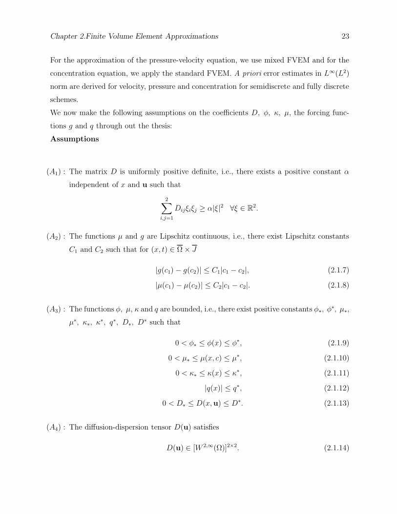
We now make the following assumptions on the coefficients D, φ, κ, µ, the forcing func-
tions g and q through out the thesis:
Assumptions
(A1) : The matrix D is uniformly positive definite, i.e., there exists a positive constant α
independent of x and u such that
2∑
i,j=1
Dijξiξj ≥ α|ξ|2 ∀ξ ∈ R2.
(A2) : The functions µ and g are Lipschitz continuous, i.e., there exist Lipschitz constants
C1 and C2 such that for (x, t) ∈ Ω × J
|g(c1) − g(c2)| ≤ C1|c1 − c2|, (2.1.7)
|µ(c1) − µ(c2)| ≤ C2|c1 − c2|. (2.1.8)
(A3) : The functions φ, µ, κ and q are bounded, i.e., there exist positive constants φ∗, φ∗, µ∗,
µ∗, κ∗, κ∗, q∗, D∗, D
∗ such that
0 < φ∗ ≤ φ(x) ≤ φ∗, (2.1.9)
0 < µ∗ ≤ µ(x, c) ≤ µ∗, (2.1.10)
0 < κ∗ ≤ κ(x) ≤ κ∗, (2.1.11)
|q(x)| ≤ q∗, (2.1.12)
0 < D∗ ≤ D(x,u) ≤ D∗. (2.1.13)
(A4) : The diffusion-dispersion tensor D(u) satisfies
D(u) ∈ [W 2,∞(Ω)]2×2. (2.1.14)
Chapter 2.Finite Volume Element Approximations 24
(A5) : The problem (2.1.1)-(2.1.6) has a unique smooth solution p, c as demanded by the
error analysis.
The authors in [20, 49, 74] have discussed existence of a unique weak solution of the above
system (2.1.1)-(2.1.6) under suitable assumptions on the data. The pressure-velocity equa-
tion is elliptic type while the concentration equation is convection dominated diffusion type.
Since in the concentration equation only velocity is present, one would like to find a good
approximation of the velocity. Therefore, for approximating velocity, it is natural to think
of some mixed methods, which provide more accurate solution for the velocity compared
to the standard finite element methods.
Earlier, Douglas et al. [37, 38], Ewing et al. [48] and Darlow et al. [31] have discussed
the mixed finite element method for approximating the velocity as well as pressure and a
standard Galerkin method for the concentration equation. They have also derived opti-
mal error estimates in L∞(L2) norm for the velocity and concentration. Moreover, in [37]
authors have proposed a modification of mixed methods when the flow is located at injec-
tion and production wells. Yang [84] has considered mixed methods with dynamic finite
element spaces, i.e., different number of elements and different basis functions are adopted
at different time levels. Compared to the conforming finite element methods (FEM), the
finite volume methods are conservative in nature and hence, they preserve the physical
conservative properties.
In this chapter, we discuss a mixed FVEM for approximating the pressure-velocity equa-
tions (2.1.1)-(2.1.2) and a standard FVEM for the approximation of the concentration
equation (2.1.3). Moreover, we present some numerical experiments to support our theo-
retical results.
This chapter is organized as follows. Section 2.1 is introductory in nature. In Section
2.2, the weak formulation for the incompressible miscible displacement problems in porous
media is described. In Section 2.3, we state and prove some auxiliary results to be used
in our subsequent analysis. The existence and uniqueness results for the discrete prob-
lem is also discussed. A priori error estimates of velocity, pressure and concentration for
the semidiscrete scheme are presented in Section 2.4. In Section 2.5, we discuss the fully
discrete scheme and derive a priori error bounds. Finally in Section 2.6, the numerical
Chapter 2.Finite Volume Element Approximations 25
procedure is discussed and some numerical experiments are conducted to substantiate the
theoretical results obtained in this chapter.
2.2 Weak formulation
Let H(div; Ω) = v = (v1, v2) ∈ (L2(Ω))2 : ∇ · v ∈ L2(Ω) be associated with the norm
‖v‖2
H(div;Ω)= ‖v‖2
(L2(Ω))2 + ‖∇ · v‖2L2(Ω), (2.2.1)
where ‖v‖2(L2(Ω))2 = ‖v1‖2 + ‖v2‖2. Further, let
U = v ∈ H(div; Ω) : v · n = 0 on ∂Ω.
The pressure-velocity equations (2.1.1)-(2.1.2) with the Neumann boundary condition (2.1.4)
has a unique solution for the pressure upto an additive constant. This non-uniqueness may
be avoided by considering the following quotient space:
W = L2(Ω)/R.
Multiply (2.1.1) and (2.1.2) by v ∈ U and w ∈ W , respectively, and integrate over Ω.
Further, use of Green’s formula and v ·n = 0 on ∂Ω, yields the following weak formulation:
Find (u, p) : J −→ U ×W satisfying
(κ−1µ(c)u,v) − (∇ · v, p) = 0 ∀v ∈ U, (2.2.2)
(∇ · u, w) = (q, w) ∀w ∈ W. (2.2.3)
Similarly, multiplying (2.1.3) by z ∈ H1(Ω) and integrating over Ω, we obtain using (2.1.5)
a weak formulation for the concentration equation (2.1.3) as follows:
Find a map c : J −→ H1(Ω) such that for t ∈ (0, T ],
(φ∂c
∂t, z) + (u · ∇c, z) + a(u; c, z) = (g(c), z) ∀z ∈ H1(Ω), (2.2.4)
c(x, 0) = c0(x) ∀x ∈ Ω,
where (·, ·) denotes the standard L2- inner product and a(u; ·, ·) : H1(Ω)×H1(Ω) −→ R is
a bilinear form defined by
a(u;φ, ψ) =
∫
Ω
D(u)∇φ · ∇ψdx ∀φ, ψ ∈ H1(Ω).
Chapter 2.Finite Volume Element Approximations 26
In fact, in order that (2.2.4) makes sense, it is necessary that u · ∇c ∈ L2(Ω).
Since D is positive definite, the bilinear form a(u; ·, ·) satisfies the following condition
a(u;φ, φ) ≥ α|φ|21 ∀φ ∈ H1(Ω), (2.2.5)
where | · |1 denotes the usual semi-norm on H1(Ω).
2.3 Finite volume element approximation
We use a mixed finite volume element method for the simultaneous approximation of ve-
locity and pressure in (2.1.1)-(2.1.2) and a standard finite volume element method for the
approximation of the concentration in (2.1.3). For this purpose, we introduce three kinds
of grids: one primal grid and two dual grids.
Let Th = T be a regular, quasi-uniform partition of the domain Ω into closed triangles
T , that is, Ω = ∪T∈ThT . Let hT = diam(T ) and h = maxT∈Th
hT . Let P1, P2 · · · , PNh
and M1,M2 · · · ,MNmdenote respectively the vertices and midpoints of the edges of the
triangles in the triangulation Th, where Nh and Nm are the total number of vertices and
total number of midpoints of the sides of the triangles of Th.Let the trial function spaces Uh and Wh associated with the approximation of velocity and
pressure respectively be the lowest order Raviart-Thomas space for triangles defined by
Uh = vh ∈ U : vh|T = (a+ bx, c + by) ∀T ∈ Th , (2.3.1)
and
Wh = wh ∈ W : wh|T is a constant ∀T ∈ Th . (2.3.2)
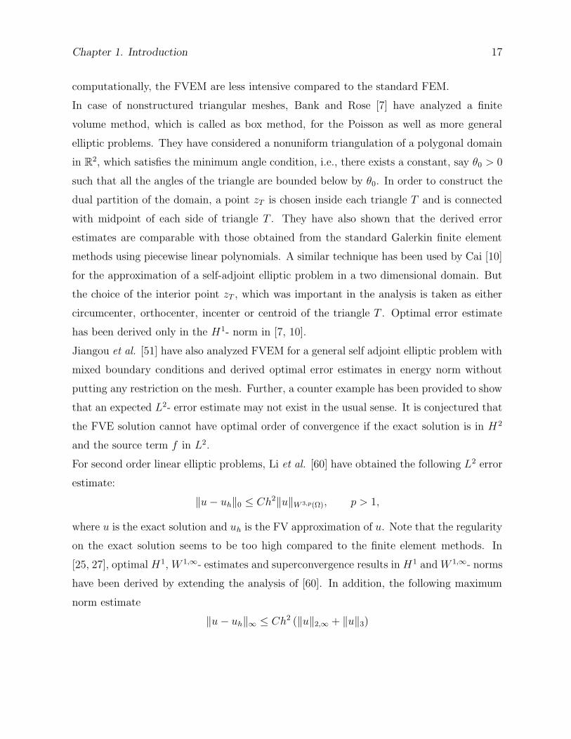
Next, we construct the dual partition for the pressure-velocity equation and the related test
spaces. The dual grid T ∗h consists of interior quadrilaterals and boundary triangles which
are constructed as follows. For an interior mid-side node, the associated dual element is a
quadrilateral. This is the union of two triangles formed by joining the end points of the side
of the triangle on which the mid-side node lies with the barycenter of the triangles which
share the mid-side node. For a mid-side node of a triangle which lies on the boundary ∂Ω,
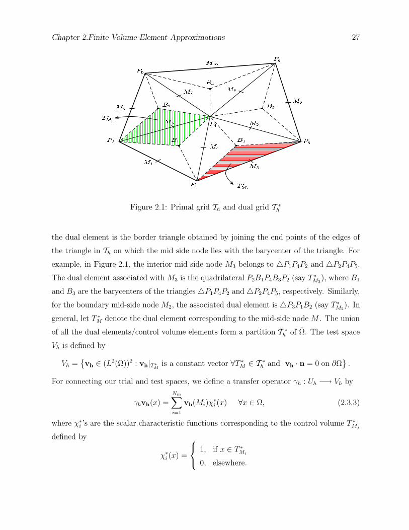
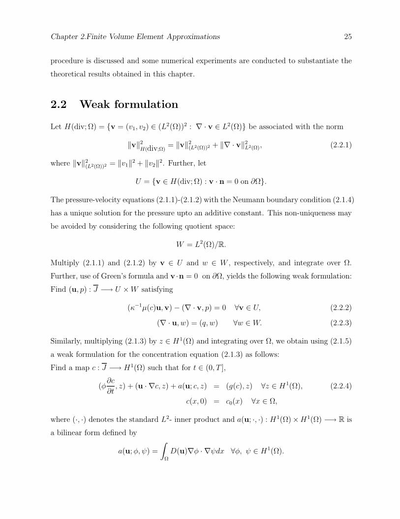
Chapter 2.Finite Volume Element Approximations 27
"!
$#
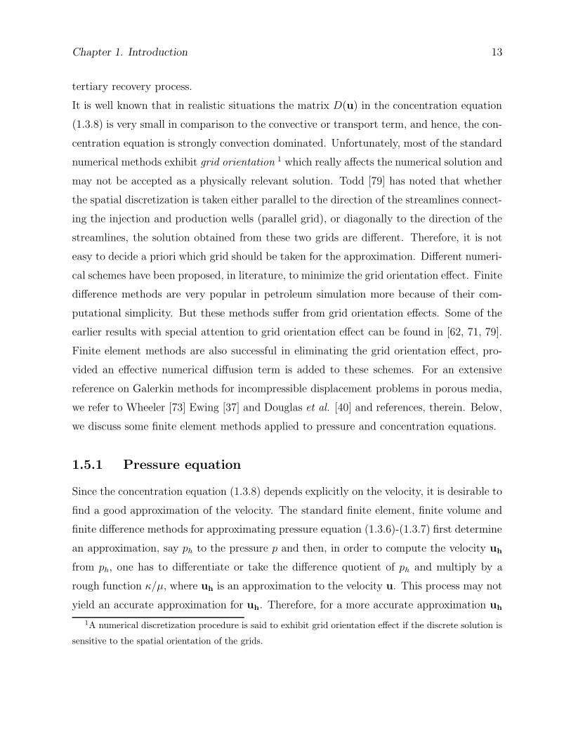
Figure 2.1: Primal grid Th and dual grid T ∗h
the dual element is the border triangle obtained by joining the end points of the edges of
the triangle in Th on which the mid side node lies with the barycenter of the triangle. For
example, in Figure 2.1, the interior mid side node M3 belongs to 4P1P4P2 and 4P2P4P5.
The dual element associated with M3 is the quadrilateral P2B1P4B3P2 (say T ∗M3
), where B1
and B3 are the barycenters of the triangles 4P1P4P2 and 4P2P4P5, respectively. Similarly,
for the boundary mid-side node M2, the associated dual element is 4P3P1B2 (say T ∗M2
). In
general, let T ∗M denote the dual element corresponding to the mid-side node M . The union
of all the dual elements/control volume elements form a partition T ∗h of Ω. The test space
Vh is defined by
Vh =
vh ∈ (L2(Ω))2 : vh|T ∗
Mis a constant vector ∀T ∗
M ∈ T ∗h and vh · n = 0 on ∂Ω
.
For connecting our trial and test spaces, we define a transfer operator γh : Uh −→ Vh by
γhvh(x) =
Nm∑
i=1
vh(Mi)χ∗i (x) ∀x ∈ Ω, (2.3.3)
where χ∗i ’s are the scalar characteristic functions corresponding to the control volume T ∗
Mj
defined by
χ∗i (x) =
1, if x ∈ T ∗Mi
0, elsewhere.

Chapter 2.Finite Volume Element Approximations 28
Multiplying (2.1.1) by γhvh ∈ Vh, integrating over the control volumes T ∗M ∈ T ∗
h , applying
the Gauss’s divergence theorem and summing up over all the control volumes, we obtain
(κ−1µ(c)u, γhvh) −Nm∑
i=1
vh(Mi) ·∫
T ∗
Mi
p nT ∗
Mids = 0 ∀vh ∈ Uh, (2.3.4)
where nT ∗
Midenotes the outward normal vector to the boundary of T ∗
Mi. Set
b(γhvh, wh) = −Nm∑
i=1
vh(Mi) ·∫
∂T ∗
Mi
wh nT ∗
Mids ∀vh ∈ Uh, ∀wh ∈ Wh. (2.3.5)
Then, the mixed FVE approximation corresponding to (2.1.1)-(2.1.2) can be written as:
find (uh, ph) : J −→ Uh ×Wh such that for t ∈ (0, T ]
(κ−1µ(ch)uh, γhvh) + b(γhvh, ph) = 0 ∀vh ∈ Uh, (2.3.6)
(∇ · uh, wh) = (q, wh) ∀wh ∈ Wh, (2.3.7)
where ch is an approximation to c obtained from (2.3.9).
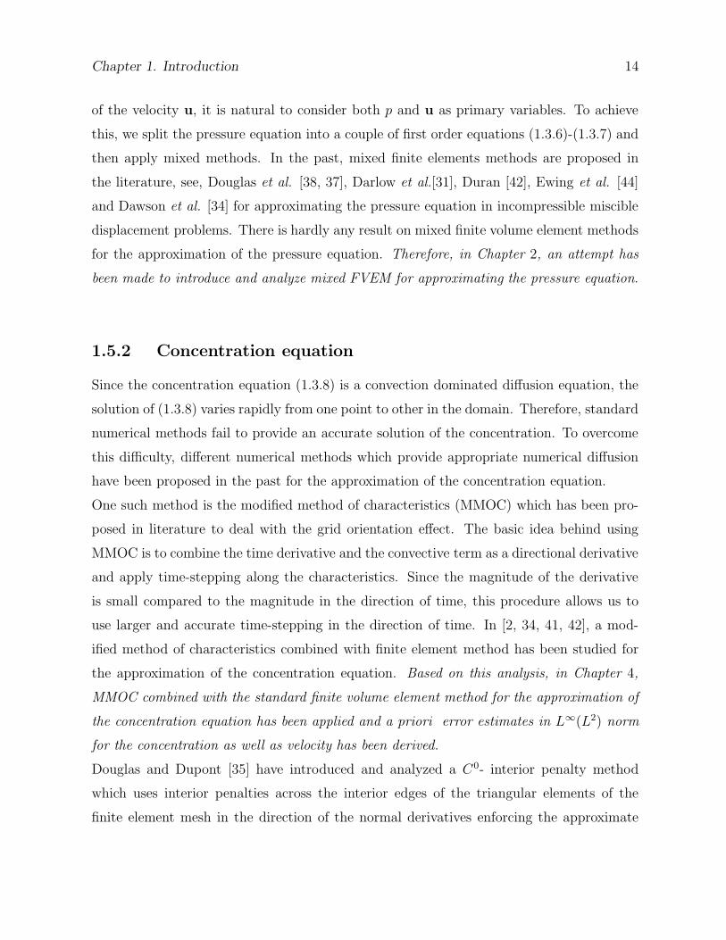
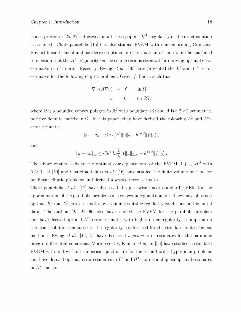
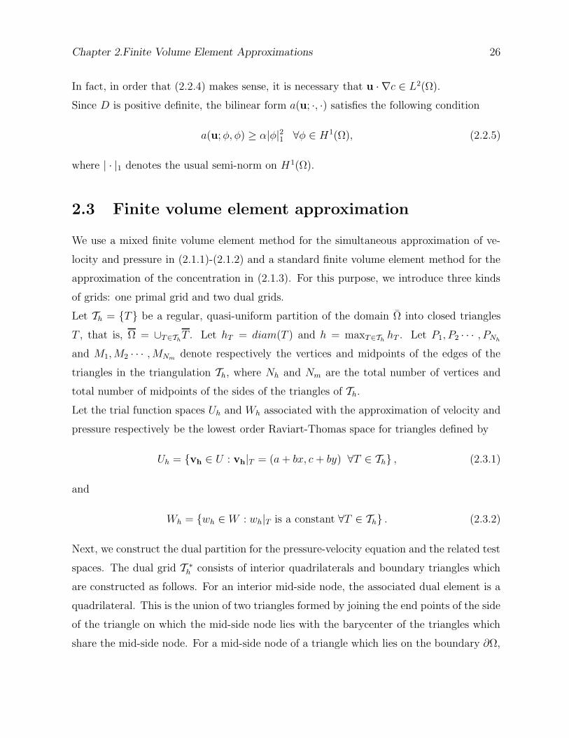
Now, we introduce a dual mesh V∗h based on Th which will be used for the approximation
of the concentration equation. For an interior vertex of Th, identify the barycenters of
the triangles in which this vertex lies and also the midpoints of the edges connecting this
vertex with the adjacent vertices. The dual element associated with the vertex is obtained
by joining successively these midpoints and the barycenters of the triangles which these
mid-side points belong to. For example, in Figure 2.2, for the interior vertex P4, the
associated dual element is M4B2M5B5M8B4M7B3M3B1M4 (say V ∗P4
). Similarly, for the
vertex on the boundary ∂Ω, say P1, the associated dual element is P1M2B2M4B1M1P1
(say V ∗P1
). In general, let V ∗P denote the dual element associated with the vertex P . The
union of all these dual elements also form a partition V∗h of Ω, corresponding to the primal
partition Th. For applying the standard finite volume element method to approximate the
concentration, we define the trial space Mh on Th and the test space Lh on V∗h as follows:
Mh =
zh ∈ C0(Ω) : zh|T ∈ P1(T ) ∀T ∈ Th
,
and
Lh =
wh ∈ L2(Ω) : wh|V ∗
Pis a constant ∀V ∗
P ∈ V∗h
.
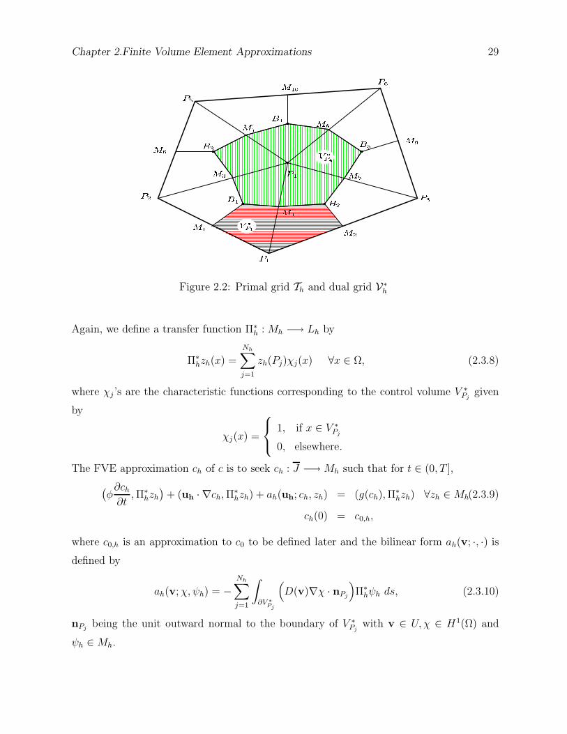
Chapter 2.Finite Volume Element Approximations 29
"!
Figure 2.2: Primal grid Th and dual grid V∗h
Again, we define a transfer function Π∗h : Mh −→ Lh by
Π∗hzh(x) =
Nh∑
j=1
zh(Pj)χj(x) ∀x ∈ Ω, (2.3.8)
where χj’s are the characteristic functions corresponding to the control volume V ∗Pj
given
by
χj(x) =
1, if x ∈ V ∗Pj
0, elsewhere.
The FVE approximation ch of c is to seek ch : J −→Mh such that for t ∈ (0, T ],
(
φ∂ch∂t
,Π∗hzh)
+ (uh · ∇ch,Π∗hzh) + ah(uh; ch, zh) = (g(ch),Π
∗hzh) ∀zh ∈ Mh(2.3.9)
ch(0) = c0,h,
where c0,h is an approximation to c0 to be defined later and the bilinear form ah(v; ·, ·) is
defined by
ah(v;χ, ψh) = −Nh∑
j=1
∫
∂V ∗
Pj
(
D(v)∇χ · nPj
)
Π∗hψh ds, (2.3.10)
nPjbeing the unit outward normal to the boundary of V ∗
Pjwith v ∈ U, χ ∈ H1(Ω) and
ψh ∈Mh.
Chapter 2.Finite Volume Element Approximations 30
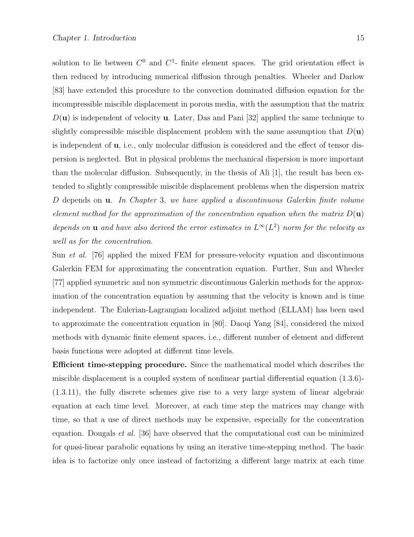
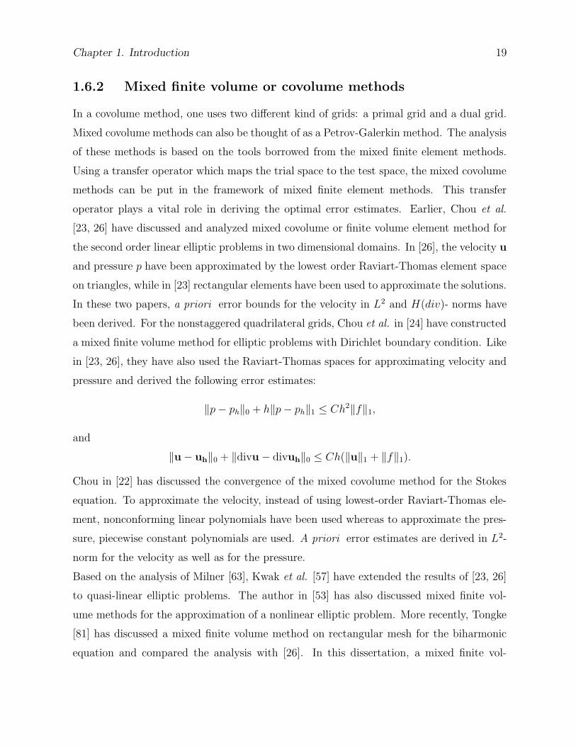
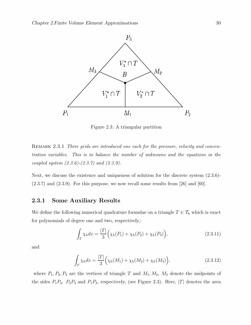
Figure 2.3: A triangular partition
Remark 2.3.1 Three grids are introduced one each for the pressure, velocity and concen-
tration variables. This is to balance the number of unknowns and the equations in the
coupled system (2.3.6)-(2.3.7) and (2.3.9).
Next, we discuss the existence and uniqueness of solution for the discrete system (2.3.6)-
(2.3.7) and (2.3.9). For this purpose, we now recall some results from [26] and [60].
2.3.1 Some Auxiliary Results
We define the following numerical quadrature formulae on a triangle T ∈ Th which is exact
for polynomials of degree one and two, respectively,:
∫
T
χhdx =|T |3
(
χh(P1) + χh(P2) + χh(P3))
, (2.3.11)
and
∫
T
χhdx =|T |3
(
χh(M1) + χh(M2) + χh(M3))
, (2.3.12)
where P1, P2, P3 are the vertices of triangle T and M1,M2, M3 denote the midpoints of
the sides P1P2, P2P3 and P1P3, respectively, (see Figure 2.3). Here, |T | denotes the area
Chapter 2.Finite Volume Element Approximations 31
of the triangle T .
We also use frequently the following trace inequality [14, pp. 417]: for w ∈ H 1(T ),
‖w‖2∂T ≤ C
(
h−1T ‖w‖2
T + hT |w|21,T)
, (2.3.13)
where ‖w‖2∂T =
∫
∂T
w2ds and ∂T denoting the boundary of the triangle T . Further, we
need the following inverse inequalities (see [29, pp. 141]):
‖χ‖1,∞ ≤ Ch−1‖χ‖1 ∀χ ∈Mh, (2.3.14)
and
‖χ‖1 ≤ Ch−1‖χ‖ ∀χ ∈Mh. (2.3.15)
By the usual interpolation theory, the operator Π∗h has the following approximation property
[27, pp. 466]:
‖χ− Π∗hχ‖0,k ≤ Chβ|χ|s,k, 0 ≤ β ≤ s ≤ 1, 1 ≤ k ≤ ∞. (2.3.16)
For our future use, let us introduce the following notations. For T ∈ Th with vertices P1, P2
and P3, set
|φh|0,h,T =
|T |3
(
φ21 + φ2
2 + φ23
)
1/2
, (2.3.17)
and
|φh|1,h,T =
(|∂φh∂x
|2 + |∂φh∂y
|2)|T |1/2
, (2.3.18)
where |T | is the area of triangle T and φj = φh(Pj), 1 ≤ j ≤ 3.
Define the discrete norms for φh ∈Mh as
‖φh‖0,h =
(
∑
T∈Th
|φh|20,h,T
)1/2
, |φh|1,h =
(
∑
T∈Th
|φh|21,h,T
)1/2
,
and
‖φh‖1,h =(
‖φh‖20,h + |φh|21,h
)1/2.
We also use the notation ‖φh‖T to denote ‖φh‖0,T =
(∫
T
φ2hdx
)1/2
.
The following lemma establishes a relation between the discrete norms and the continuous
norms on the Sobolev spaces.
Chapter 2.Finite Volume Element Approximations 32
Lemma 2.3.1 [60, pp. 124] For φh ∈Mh, | · |1,h and | · |1 are identical. Further, ‖ ·‖0,h and
‖ · ‖1,h are equivalent to ‖ · ‖ and ‖ · ‖1, respectively, that is, there exist positive constants
C3, · · · , C6 > 0, independent of h, such that
C3‖φh‖0,h ≤ ‖φh‖ ≤ C4‖φh‖0,h ∀φh ∈Mh, (2.3.19)
and
C5||φh||1,h ≤ ||φh||1 ≤ C6||φh||1,h ∀φh ∈Mh. (2.3.20)
Proof. Since∂φh∂x
and∂φh∂y
are constants on a triangle T , the norms | · |1 and | · |1,h are
identical. Now using the quadrature formula (2.3.12), we obtain
‖φh‖2T =
∫
T
|φh|2dx =|T |3
(
φh(M1)2 + φh(M2)
2 + φh(M3)2)
=|T |3
[
(
φ1 + φ2
2
)2
+
(
φ2 + φ3
2
)2
+
(
φ1 + φ3
2
)2]
=|T |12
[
φ21 + φ2
2 + φ23 + (φ1 + φ2 + φ3)
2]
. (2.3.21)
Using Young’s inequality (1.2.4) with ε = 1, (2.3.21) can be written as
‖φh‖2T =
|T |12
[
2(φ21 + φ2
2 + φ23) + 2φ1φ2 + 2φ2φ3 + 2φ1φ3
]
≤ |T |4
[
φ21 + φ2
2 + φ23
]
. (2.3.22)
A use of (2.3.17) yields
‖φh‖2 ≤ ‖φh‖20,h. (2.3.23)
From (2.3.23) and (2.3.21), we find that
1
4‖φh‖2
0,h ≤ ‖φh‖2 ≤ ‖φh‖20,h. (2.3.24)
Now the estimate (2.3.20) follows from (2.3.24) and the fact that |·|1 and |·|1,h are identical.
This completes the proof.
Chapter 2.Finite Volume Element Approximations 33
Lemma 2.3.2 The following results hold true for ∀φh ∈ Mh,∫
T
(φh − Π∗hφh) dx = 0 ∀T ∈ Th, (2.3.25)
and∫
∂T
(φh − Π∗hφh) ds = 0 (2.3.26)
Proof. Since φh is linear on each triangle T , from (2.3.11), we obtain
∫
T
(φh − Π∗hφh)dx =
∫
T
φhdx−3∑
i=1
∫
V ∗
i ∩T
Π∗hφhdx
=
∫
T
φhdx−3∑
i=1
φi|V ∗i ∩ T |,
where |V ∗i ∩ T | denotes the area of the control volume V ∗
i ∩ T .
Since |V ∗i ∩ T | =
|T |3, i = 1, 2, 3, we find that
∫
T
(φh − Π∗hφh)dx =
|T |3
(φ1 + φ2 + φ3) −3∑
i=1
φi|T |3
= 0.
This proves (2.3.25). Now (ii) follows directly from the definition of Π∗h and this completes
the rest of the proof.
Now introduce the following function
εh(ψ, χh) = (ψ, χh) − (ψ,Π∗hχh) ∀χh ∈Mh. (2.3.27)
Lemma 2.3.3 [68, pp. 40] Let z ∈ P1(T ) and zT be the average of z on T , i.e., zT =1
|T |
∫
T
z dx. Then
‖z − zT ‖0,T ≤ ChT |∇z|0,T . (2.3.28)
Proof. Let v = z − zT , then∫
T
v dx =
∫
T
(z − zT )dx =
∫
T
z dx−∫
T
zT dx = 0.
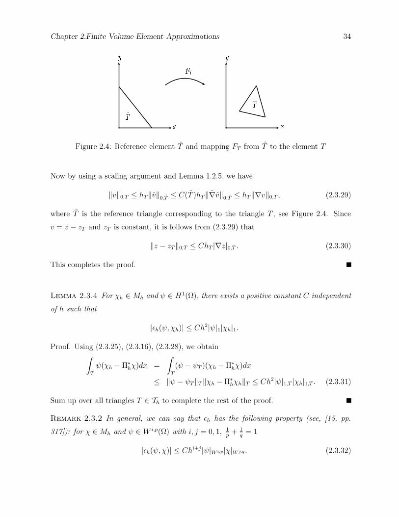
Chapter 2.Finite Volume Element Approximations 34
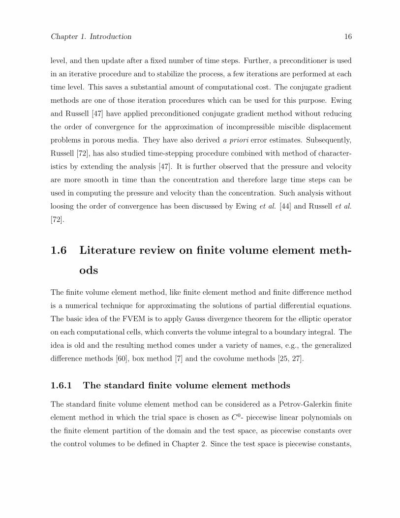
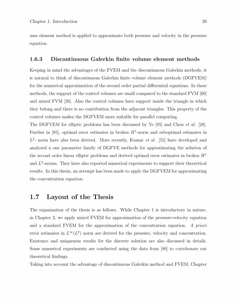
Figure 2.4: Reference element T and mapping FT from T to the element T
Now by using a scaling argument and Lemma 1.2.5, we have
‖v‖0,T ≤ hT‖v‖0,T ≤ C(T )hT‖∇v‖0,T ≤ hT‖∇v‖0,T , (2.3.29)
where T is the reference triangle corresponding to the triangle T , see Figure 2.4. Since
v = z − zT and zT is constant, it is follows from (2.3.29) that
‖z − zT ‖0,T ≤ ChT |∇z|0,T . (2.3.30)
This completes the proof.
Lemma 2.3.4 For χh ∈Mh and ψ ∈ H1(Ω), there exists a positive constant C independent
of h such that
|εh(ψ, χh)| ≤ Ch2|ψ|1|χh|1.
Proof. Using (2.3.25), (2.3.16), (2.3.28), we obtain∫
T
ψ(χh − Π∗hχ)dx =
∫
T
(ψ − ψT )(χh − Π∗hχ)dx
≤ ‖ψ − ψT‖T‖χh − Π∗hχh‖T ≤ Ch2|ψ|1,T |χh|1,T . (2.3.31)
Sum up over all triangles T ∈ Th to complete the rest of the proof.
Remark 2.3.2 In general, we can say that εh has the following property (see, [15, pp.
317]): for χ ∈Mh and ψ ∈ W i,p(Ω) with i, j = 0, 1, 1p
+ 1q
= 1
|εh(ψ, χ)| ≤ Chi+j|ψ|W i,p|χ|W j,q . (2.3.32)
Chapter 2.Finite Volume Element Approximations 35
Lemma 2.3.5 [76, pp. 332] The matrix D(u) defined in (1.3.3) is uniformly Lipschitz
continuous, i.e., there exists a constant C such that for u and v ∈ (L2(Ω))2,
‖D(u) −D(v)‖(L2(Ω))2×2 ≤ C‖u − v‖(L2(Ω))2 . (2.3.33)
Proof. Using (1.2.1) and (1.3.3), we obtain
|D(u) −D(v)|1 =
2∑
i=1
maxj=1,2
|D(u)i,j −D(v)i,j|
≤2∑
i=1
maxj=1,2
|φ(x)|∣
∣
∣
∣
(dl − dt)
(
uiuj|u| − vivj
|v|
)
+ dtδij(|u| − |v|)∣
∣
∣
∣
.
Using (2.1.9), we find that
|D(u) −D(v)|1 ≤ φ∗
(
2∑
i=1
|dl − dt|maxj=1,2
∣
∣
∣
∣
uiuj|u| − vivj
|v|
∣
∣
∣
∣
+ 2dt ||u| − |v||)
.
Note that
uiuj|u| − vivj
|v| =uiuj|u| − uivj
|u| +uivj|u| − uivj
|v| +uivj|v| − vivj
|v|
=ui(uj − vj)
|u| +uivj(|v| − |u|)
|u||v| +vj(ui − vi)
|v|≤ 2|u − v| + (|v| − |u|)
≤ 3|u − v|.
Hence,
|D(u) −D(v)|1 ≤ 2K1(dt + 3|dl − dt|)|u− v|. (2.3.34)
Using (1.2.3) and (2.3.34), we obtain
|D(u) −D(v)|2 ≤ 21/2|D(u) −D(v)|1 ≤ 23/2K1(dl + 3|dl − dt|)|u − v|. (2.3.35)
Now integrate over Ω to complete the rest of the proof.
The following lemma yields a relation between the bilinear forms a(u; ·, ·) and ah(u; ·, ·),the proof of which is based on the ideas of a similar result in [46, pp. 1871].
Chapter 2.Finite Volume Element Approximations 36
Lemma 2.3.6 Assume that χh, ψh ∈Mh. Then
ah(u;χh, ψh) = a(u;χh, ψh) +∑
T∈Th
∫
∂T
(D(u)∇χh · n)(Π∗hψh − ψh)ds
+∑
T∈Th
∫
T
∇ · (D(u)∇χh)(ψh − Π∗hψh)dx. (2.3.36)
Moreover, the following inequality holds:
ah(u;χh, ψh) ≥ a(u;χh, ψh) − Ch|ψh|1|φh|1. (2.3.37)
Proof. A use of Gauss’s divergence theorem on each of V ∗j ∩ T, (j = 1, 2, 3), (see Figure
2.3) yields
ah(u;χh, ψh) = −∑
T∈Th
3∑
j=1
Π∗hψh
∫
∂V ∗
j ∩T
(D(u)∇χh) · n ds, (2.3.38)
with n denoting the unit outward normal to ∂V ∗j ∩ T . Now (2.3.38) can be rewritten as:
ah(u;χh, ψh) =∑
T∈Th
3∑
j=1
Π∗hψh
∫
PjPj+1
(D(u)∇χh) · n ds
−∑
T∈Th
3∑
j=1
∫
V ∗
j ∩T
Π∗hψh∇ · (D(u)∇χh) dx
=∑
T∈Th
∫
∂T
(Π∗hψh − ψh)(D(u)∇χh) · n ds+
∑
T∈Th
∫
∂T
ψh(D(u)∇χh) · n ds
−∑
T∈Th
3∑
j=1
∫
V ∗
j ∩T
Π∗hψh∇ · (D(u)∇χh) dx.
Applying Green’s formula on triangle T for the second term, we obtain
ah(u;χh, ψh) =∑
T∈Th
∫
∂T
(Π∗hψh − ψh)(D(u)∇χh) · n ds+
∑
T∈Th
∫
T
D(u)∇χh · ∇ψh dx
+∑
T∈Th
∫
T
∇ · (D(u)∇χh)ψh dx−∑
T∈Th
3∑
j=1
∫
V ∗
j ∩T
Π∗hψh∇ · (D(u)∇χh) dx
=∑
T∈Th
∫
∂T
(Π∗hψh − ψh)(D(u)∇χh) · n ds+
∑
T∈Th
∫
T
D(u)∇χh · ∇ψh dx
+∑
T∈Th
∫
T
∇ · (D(u)∇χh)(ψh − Π∗hψh) dx.
Chapter 2.Finite Volume Element Approximations 37
This proves (2.3.36). To prove (2.3.37), we first use (2.3.26) to obtain
∑
T∈Th
∫
∂T
(Π∗hψh − ψh)(D(u)∇χh) · nds =
∑
T∈Th
∫
∂T
(Π∗hψh − ψh)(D −DT ) · ∇χh.n ds,
where DT = D(xc), xc ∈ ∂T . Since |D − DT |∞ ≤ Ch‖D‖1,∞ (see [46, pp. 1873]), we
have
∑
T∈Th
∫
∂T
(Π∗hψh − ψh)(D(u)∇χh) · n ds ≤ Ch‖D‖1,∞
∑
T∈Th
∫
∂T
(Π∗hψh − ψh)∇χh.n ds.
(2.3.39)
Using the Cauchy-Schwarz inequality, the trace inequality (2.3.13) and (2.3.16) in (2.3.39),
we arrive at
∑
T∈Th
∫
∂T
(Π∗hψh − ψh)(D(u)∇χh) · n ds ≤ Ch‖D‖1,∞
(
∑
T∈Th
∫
∂T
|Π∗hψh − ψh|2ds
)1/2
(
∑
T∈Th
∫
∂T
|∇χh · n|2ds)1/2
≤ Ch
(
∑
T∈Th
h−1‖Π∗hψh − ψh‖2
T + h|Π∗hψh − ψh|21,T )
)1/2(∑
T∈Th
h−1|∇χh|21,T + h|χh|22,T
)1/2
≤ Ch
(
∑
T∈Th
|ψh|21,T
)1/2(∑
T∈Th
|χh|21,T
)1/2
≤ Ch|ψh|1|χh|1. (2.3.40)
In the last inequality, we have used the fact that χh is linear on triangle T , i.e., |χh|2,T = 0.
Again use |χh|2,T = 0, the Cauchy-Schwarz inequality and (2.3.16) to obtain
∑
T∈Th
∫
T
∇ · (D(u)∇χh)(ψh − Π∗hψh)dx ≤ ‖D‖1,∞
(
∑
T∈Th
∫
T
|∇χh|2dx)1/2
(
∑
T∈Th
∫
T
|ψh − Π∗hψh|2dx
)1/2
≤ Ch|χh|1|ψh|1. (2.3.41)
Now (2.3.37) follows from (2.3.40) and (2.3.41). This completes the proof.
Chapter 2.Finite Volume Element Approximations 38
Remark 2.3.3 : Note that (2.3.36) also holds true for χ ∈ H1(Ω).
Lemma 2.3.7 Under the assumption that the matrix D is positive definite, there exists a
positive constant α0 independent of h such that
ah(uh;χh, χh) ≥ α0|χh|21 ∀χh ∈Mh. (2.3.42)
Proof. Since the matrix D is uniformly positive, we find that
a(uh;χh, χh) ≥ α|χh|21. (2.3.43)
Use (2.3.37) and (2.3.43) to obtain
ah(uh;χh, χh) ≥ α|χh|21 − Ch|χh|21. (2.3.44)
Choose h small so that α− Ch = α0 > 0 and this completes the rest of the proof.
Lemma 2.3.8 [60, pp. 240 ] The operator Π∗h has the following properties.
(i) For Π∗h : Mh −→ Lh defined in (2.3.8)
(φh,Π∗hψh) = (ψh,Π
∗hφh) ∀φh, ψh ∈Mh. (2.3.45)
(ii) With ‖|φh‖| = (φh,Π∗hφh)
1/2, the norms ‖| · ‖| and ‖ · ‖ are equivalent on Uh, that is,
there exist positive constants C7 and C8, independent of h, such that
C7||φh|| ≤ ‖|φh‖| ≤ C8||φh|| ∀φh ∈Mh. (2.3.46)
(iii) Π∗h is stable with respect to the L2 norm, i.e., there exists a positive constant C
independent of h such that
‖Π∗hχh‖ ≤ C‖χh‖ ∀χh ∈Mh. (2.3.47)
Proof. To prove (i), we note that
(φh,Π∗hψh) =
∑
T∈Th
3∑
j=1
∫
V ∗
j ∩T
φh Π∗hψh dx.
Chapter 2.Finite Volume Element Approximations 39
Using the definition of Π∗h and the quadrature formula (2.3.11), we obtain with φj = φh(Pj)
3∑
j=1
∫
Vj∩T
φhΠ∗hψhdx = ψ1
∫
V ∗
1∩T
φhdx+ ψ2
∫
V ∗
2∩T
φhdx+ ψ3
∫
V ∗
3∩T
φhdx
= ψ1 (2φ1 + φh(M1) + φh(M3) + 2φh(B))|V ∗
1 ∩ T |6
+ψ2 (2φ2 + φh(M1) + φh(M2) + 2φh(B))|V ∗
2 ∩ T |6
+ψ3 (2φ3 + φh(M2) + φh(M3) + 2φh(B))|V ∗
3 ∩ T |6
.
Using φh(B) =φ1 + φ2 + φ3
3and φh(Mi) =
φi+1 + φi2
, i = 1, 2, 3, φ4 = φ1, we find that
3∑
j=1
∫
Vj∩T
φhΠ∗hψhdx =
|T |108
[
ψ1(22φ1 + 7φ2 + 7φ3) + ψ2 (22φ2 + 7φ1 + 7φ3)
+ψ3 (22φ3 + 7φ1 + 7φ2)]
=|T |54
[ψ1, ψ2, ψ3]
22 7 7
7 22 7
7 7 22
[φ1, φ2, φ3]T ,
where we have used the fact that |V ∗j ∩ T | =
|T |3, j = 1, 2, 3, see Figure 2.3. This proves
that the inner product (·, γ·) is symmetric.
For (ii) that is for the equivalence of the norms, we now rewrite
3∑
j=1
γφh|V ∗
j
∫
V ∗
j ∩T
φhdx =|T |108
[
22(φ21 + φ2
2 + φ23) + 14(φ1φ2 + φ2φ3 + φ1φ3)
]
=|T |54
[
15(φ21 + φ2
2 + φ23) + 7(φ1 + φ2 + φ3)
2]
. (2.3.48)
The equivalence of the norms follow from (2.3.48) and (2.3.21). This completes the proof
of (ii).
In order to prove (iii), we note that
‖Π∗hχh‖2 =
∑
T∈Th
3∑
j=1
∫
V ∗
j ∩T
|Π∗hχh|2dx.
Chapter 2.Finite Volume Element Approximations 40
Now using the definition of Π∗h, we obtain
3∑
j=1
∫
V ∗
j ∩T
|Π∗hχh|2dx =
3∑
j=1
χ2j |V ∗
j ∩ T |
=3∑
j=1
χ2j
|T |3. (2.3.49)
Now (iii) follows from (2.3.21) and (2.3.49). This completes the rest of the proof.
Lemma 2.3.9 [26, pp. 1854] The operator γh defined in (2.3.3) has the following proper-
ties:
(a) ‖γhvh‖(L2(Ω))2 ≤ ‖vh‖(L2(Ω))2 ∀vh ∈ Uh, (2.3.50)
(b) ‖vh − γhvh‖(L2(Ω))2 ≤ Ch‖vh‖H(div;Ω). (2.3.51)
(c) b(γhvh, wh) = −(∇ · vh, wh) ∀vh ∈ Uh, ∀wh ∈ Wh. (2.3.52)
(d) There exists a positive constant C which depends on the bounds of κ−1 and µ and is
independent of h such that
(
κ−1µ(ch)vh, γhvh
)
≥ C‖vh‖2H(div;Ω) ∀vh ∈ Uh, (2.3.53)
with ∇ · vh=0.
Proof. Since vh is linear on triangle T , (a) can be proved in the same way as we have
proved (iii) of Lemma 2.3.8. To prove (b), we proceed as follows. Note that
‖vh − γhvh‖2(L2(Ω))2 =
∑
T∈Th
∫
T
|vh − γhvh|2dx. (2.3.54)
Using the definition of γh and referring to Figure 2.5, for vh = (v1h, v
2h), we obtain
∫
T
|vh − γhvh|2dx =
3∑
j=1
∫
4Pj+1BPj
|vh(x) − γhvh(x)|2dx
=
3∑
j=1
∫
4Pj+1BPj
|vh(x) − vh(Mj)|2dx
=3∑
j=1
∫
4Pj+1BPj
2∑
k=1
(|vkh(x) − vkh(Mj)|2dx.
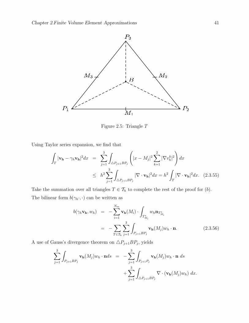
Chapter 2.Finite Volume Element Approximations 41
Figure 2.5: Triangle T
Using Taylor series expansion, we find that
∫
T
|vh − γhvh|2dx =3∑
j=1
∫
4Pj+1BPj
(
|x−Mj|22∑
k=1
|∇vkh|2)
dx
≤ h2
3∑
j=1
∫
4Pj+1BPj
|∇ · vh|2dx = h2
∫
T
|∇ · vh|2dx. (2.3.55)
Take the summation over all triangles T ∈ Th to complete the rest of the proof for (b).
The bilinear form b(γh·, ·) can be written as
b(γhvh, wh) = −Nm∑
i=1
vh(Mi) ·∫
T ∗
Mi
whnT ∗
Mi
= −∑
T∈Th
3∑
j=1
∫
Pj+1BPj
vh(Mj)wh · n. (2.3.56)
A use of Gauss’s divergence theorem on 4Pj+1BPj, yields
3∑
j=1
∫
Pj+1BPj
vh(Mj)wh · nds = −3∑
j=1
∫
Pj+1Pj
vh(Mj)wh · n ds
+3∑
j=1
∫
4Pj+1BPj
∇ · (vh(Mj)wh) dx.
Chapter 2.Finite Volume Element Approximations 42
Using the fact that vh is linear on each triangle and Mj is the mid point of PjPj+1, we find
that
3∑
j=1
∫
Pj+1BPj
vh(Mj)wh · n = −3∑
j=1
∫
Pj+1Pj
vh(Mj)wh · n ds = −3∑
j=1
wh(vh(Mj) · n) |PjPj+1|
= −3∑
j=1
whvh(Pj) + vh(Pj+1)
2· n |PjPj+1|
= −3∑
j=1
∫
PjPj+1
whvh · n ds
= −∑
∂T
whvh · n ds = −wh∫
T
∇ · vh dx. (2.3.57)
This completes the proof for (c).
Since ∇ · vh = 0, to prove (2.3.53), it is enough to show that
(vh, γhvh) ≥ C‖vh‖(L2(Ω))2 . (2.3.58)
This can be proved using the same arguments as in the proof of (i) and (ii) in Lemma
2.3.8. This completes the proof.
Lemma 2.3.10 [19, pp. 130] There exists a positive constant β independent of h such that
the following inf-sup condition holds true:
sup06=vh∈Uh
(∇ · vh, wh)
‖vh‖H(div;Ω)
≥ β‖wh‖ ∀wh ∈ Wh. (2.3.59)
2.3.2 Existence and Uniqueness of Discrete Solution
Using (2.3.52), the problem (2.3.6)-(2.3.7) yields a system of linear algebraic equations for
a given ch. To show the existence of a solution, it is enough to prove the uniqueness of the
solution of the corresponding homogeneous system
(κ−1µ(ch)uh, γhvh) − (∇ · vh, ph) = 0 ∀vh ∈ Uh, (2.3.60)
(∇ · uh, wh) = 0 ∀wh ∈ Wh. (2.3.61)
For uniqueness, it is sufficient to show that uh = 0, ph = 0. Substitute wh = ∇ · uh in
(2.3.61) to obtain ∇ · uh = 0. Put wh = ph in (2.3.61) and vh = uh in (2.3.60) and use
Chapter 2.Finite Volume Element Approximations 43
(2.3.53) to obtain
‖uh‖H(div;Ω)= 0.
This implies that uh = 0. Use uh = 0 in (2.3.60) and the inf-sup condition (2.3.59), to find
that ph = 0. Hence, for a given ch, there exists a unique solution(
uh(ch),ph(ch))
satis-
fying (2.3.6)-(2.3.7). On substituting in (2.3.9), we obtain a system of nonlinear ordinary
differential equations in ch. An appeal to Picard’s Theorem yields the existence of a unique
solution in (0, th) for some 0 < th ≤ T . To continue the solution for all t ∈ J , we need an
a priori bound for ch. Now the quasi-uniformity of the mesh implies that
‖uh‖(L∞(Ω))2 ≤ Ch−1‖uh‖(L2(Ω))2 . (2.3.62)
For a priori bound, choose zh = ch in (2.3.9) and use (2.3.62) to bound uh. Then a use of
Lemma 2.3.8 yields
1
2
d
dt(φch,Π
∗hch) + ah(uh; ch, ch) ≤ S(h)‖ch‖2, (2.3.63)
where S(h) = O(h−1). For a given uh, the positive-definiteness of ah(uh; ch, ch) given in
(2.3.42) with (2.1.9) yields a priori estimates in L2 and H1- norms for ch. Now the a priori
bound ‖ch‖L∞(L2) can be used to show the existence of an uniqueness solution ch of the
concentration equation for all t ∈ J and for a fixed h. This completes the part of unique
solvability of (2.3.6)-(2.3.7) and (2.3.9).
2.4 Error estimates
In this section, we discuss the error estimates for the semidiscrete method. First of all,
we derive the estimates for the velocity and pressure in terms of the concentration using
the Raviart- Thomas projection and L2 projection. Then for finding the estimates for the
concentration, we split c − ch = (c − Rhc) + (Rhc − ch), where Rh is the Ritz projection
to be defined in (2.4.27) . In Lemma 2.4.1 and Lemma 2.4.3, we derive, respectively, H 1
and L2- error estimates for Rh. Based on these estimates, we finally obtain a priori error
estimates for the concentration in L∞(L2)- norm.
Chapter 2.Finite Volume Element Approximations 44
2.4.1 Estimates for the velocity
Let Πh be the usual Raviart-Thomas projection Πh : U −→ Uh defined by
(∇ · (u − Πhu), wh) = 0 ∀wh ∈ Wh, (2.4.1)
which has the following approximation properties (see [19, pp. 163]):
‖u − Πhu‖(L2(Ω))2 ≤ Ch‖u‖(H1(Ω))2 , (2.4.2)
‖∇ · (u − Πhu)‖ ≤ Ch‖∇ · u‖H1(Ω), (2.4.3)
and (see [58, pp. 48])
‖u − Πhu‖(L∞(Ω))2 ≤ Ch‖u‖(W 1,∞(Ω))2 . (2.4.4)
Let Ph be the L2- projection of W onto Wh defined by
(p− Php, wh) = 0 ∀wh ∈ Wh. (2.4.5)
The operator Ph satisfies the following approximation property (see [19, pp. 163]):
‖p− Php‖ ≤ Ch‖p‖H1(Ω). (2.4.6)
Further, the following inverse property holds:
‖vh‖(L∞(Ω))2 ≤ Ch−1‖vh‖(L2(Ω))2 ∀vh ∈ Uh. (2.4.7)
Now, we introduce the following auxiliary functions (uh, ph) : [0, T ] −→ Uh×Wh satisfying
(κ−1µ(c)uh,vh) − (∇ · vh, ph) = 0 ∀vh ∈ Uh, (2.4.8)
(∇ · uh, wh) = (q, wh) ∀wh ∈ Wh. (2.4.9)
For a proof of the the existence and uniqueness of the solution of (2.4.8)-(2.4.9), we refer
to [9, pp. 52]. The following error estimates for (uh, ph) can be obtained by using the
properties of Raviart-Thomas projection Πh and L2 projection Ph defined in (2.4.1) and
(2.4.5), respectively:
‖u − uh‖(L2(Ω))2 + ‖p− ph‖ ≤ Ch(
‖u‖(H1(Ω))2 + ‖p‖1
)
, (2.4.10)
Chapter 2.Finite Volume Element Approximations 45
and
‖∇ · (u − uh)‖ ≤ Ch‖∇ · u‖1, (2.4.11)
where the constant C is independent of h, but may depend on the bounds of µ and κ−1
given in (2.1.10) and (2.1.11). For a proof, see [19, pp. 166].
The bound for uh in L∞- norm can be found by using (2.4.2), (2.4.4), (2.4.7) and (2.4.10)
as follows:
‖uh‖(L∞(Ω))2 ≤ ‖u − uh‖(L∞(Ω))2 + ‖u‖(L∞(Ω))2
≤ ‖u − Πhu‖(L∞(Ω))2 + ‖Πhu − uh‖(L∞(Ω))2 + ‖u‖(L∞(Ω))2
≤ C(
h‖u‖(W 1,∞(Ω))2 + h−1‖Πhu − uh‖(L2(Ω))2 + ‖u‖(L∞(Ω))2)
≤ C(
h‖u‖(W 1,∞(Ω))2 + h−1‖Πhu − u‖(L2(Ω))2
+h−1‖u − uh‖(L2(Ω))2 + ‖u‖(L∞(Ω))2
)
≤ C(
h‖u‖(W 1,∞(Ω))2 + ‖u‖(H1(Ω))2 + ‖p‖1 + ‖u‖(L∞(Ω))2
)
. (2.4.12)
Theorem 2.4.1 Assume that the triangulation Th is quasi-uniform. Let (u, p) and (uh, ph),
respectively, be the solutions of (2.2.2)-(2.2.3) and (2.3.6)-(2.3.7). Then, there exists a pos-
itive constant C, independent of h, but dependent on the bounds of κ−1 and µ such that
‖u − uh‖(L2(Ω))2 + ‖p− ph‖ ≤ C[
‖c− ch‖ + h(‖u‖(H1(Ω))2 + ‖p‖1)]
, (2.4.13)
and
‖∇ · (u − uh)‖ ≤ Ch‖∇ · u‖1, (2.4.14)
provided u(t) ∈ (H1(Ω))2, ∇ · u(t) ∈ H1(Ω) and p(t) ∈ H1(Ω).
Proof. Write u − uh = (u − uh) + (uh − uh) and p− ph = (p− ph) + (ph − ph). Since the
estimates of u− uh and p− ph are known from (2.4.10), it is sufficient to estimate uh−uh
and ph − ph . Let e1h = uh − uh and e2h = ph − ph. Using (2.3.52) in (2.3.6)-(2.3.7), we
obtain
(κ−1µ(ch)uh, γhvh) − (∇ · vh, ph) = 0 ∀vh ∈ Uh, (2.4.15)
(∇ · uh, wh) = (q, wh) ∀wh ∈ Wh. (2.4.16)
Chapter 2.Finite Volume Element Approximations 46
Subtracting (2.4.15) from (2.4.8) and (2.4.16) from (2.4.9), we find that
(κ−1µ(ch)e1h, γhvh) − (∇ · vh, e2h) = −(κ−1µ(c)uh,vh − γhvh)
−(κ−1(µ(c) − µ(ch))uh, γhvh) ∀vh ∈ Uh, (2.4.17)
(∇ · e1h, wh) = 0 ∀wh ∈ Wh. (2.4.18)
Since ∇ · Uh ⊂ Wh, take wh = ∇ · e1h in (2.4.18) to arrive at
‖∇ · e1h‖ = 0, (2.4.19)
and hence, using (2.2.1), we obtain
‖e1h‖H(div;Ω)= ‖e1h‖(L2(Ω))2 . (2.4.20)
Choosing vh = e1h in (2.4.17) and wh = e2h in (2.4.18), we arrive at
(κ−1µ(ch)e1h, γhe1h) = −(κ−1µ(c)uh, e1h − γhe1h) − (κ−1(µ(c) − µ(ch))uh, γhe1h).
Using (2.3.51), (2.3.53) with (2.1.10)-(2.1.11) and (2.1.8), we obtain
‖e1h‖2
H(div;Ω)≤ C
(
‖uh‖(L2(Ω))2‖e1h − γhe1h‖(L2(Ω))2 + ‖c− ch‖‖uh‖(L∞(Ω))2‖e1h‖(L2(Ω))2
)
≤ C(
h‖uh‖(L2(Ω))2‖e1h‖H(div;Ω)+ ‖c− ch‖‖uh‖(L∞(Ω))2‖e1h‖(L2(Ω))2
)
.
(2.4.21)
Substitute (2.4.21) in (2.4.20) to find that
‖e1h‖(L2(Ω))2 ≤ C(
h‖uh‖(L2(Ω))2 + ‖c− ch‖‖uh‖(L∞(Ω))2
)
. (2.4.22)
For estimating e2h, choose vh = e1h in (2.4.17), use (2.1.10)-(2.1.11), (2.1.8) and (2.4.20)
to obtain
(∇ · e1h, e2h) ≤ C(
h‖uh‖(L2(Ω))2 + ‖c− ch‖‖uh‖(L∞(Ω))2
+‖e1h‖(L2(Ω))2
)
‖e1h‖(L2(Ω))2 . (2.4.23)
A use of the inf-sup condition (2.3.59) on the left hand side of (2.4.23) yields
‖e2h‖ ≤ C(
h‖uh‖(L2(Ω))2 + ‖c− ch‖‖uh‖(L∞(Ω))2 + ‖e1h‖(L2(Ω))2
)
. (2.4.24)
Chapter 2.Finite Volume Element Approximations 47
Using (2.4.10), (2.4.12), (2.4.22) and (2.4.24) can be written as
‖e1h‖(L2(Ω))2 ≤ C(
h‖u‖(H1(Ω))2 + ‖c− ch‖)
, (2.4.25)
and
‖e2h‖ ≤ C(
h‖u‖(H1(Ω))2 + ‖c− ch‖)
, (2.4.26)
where the constant C depends on ‖uh‖(L∞(Ω))2 derived in (2.4.12). An application of the
triangle inequality completes the proof of (2.4.13). Now the estimate for (2.4.14) directly
follows from (2.4.19) and (2.4.11). This completes the rest of the proof.
2.4.2 Estimates for the concentration
Let Rh : H1(Ω) −→Mh be the projection of c defined by
A(u; c−Rhc, χ) = 0 ∀χ ∈Mh, (2.4.27)
where
A(u;ψ, χ) = ah(u;ψ, χ) + (u · ∇ψ, χ) + (λψ, χ) ∀χ ∈Mh. (2.4.28)
The function λ is chosen in such a way that A(·; ·, ·) is coercive.
Since
(u · ∇ψ, ψ) =
∫
Ω
ψu · ∇ψdx = −∫
Ω
∇ · (ψu)ψdx+
∫
∂Ω
u · nψ2dx
= −∫
Ω
∇ · (ψu)ψdx = −∫
Ω
ψu · ∇ψdx−∫
Ω
∇ · uψ2dx,
we obtain
(u · ∇ψ, ψ) = −1
2(∇ · u, ψ2) = −1
2(q, ψ2). (2.4.29)
If we choose λ = 1 + 12q, then (u · ∇χ, χ) + (λχ, χ) = (χ, χ) for χ ∈Mh.
Now we derive the error bound in H1 and L2 norms for c−Rhc. Let Ih be the continuous
interpolant onto Mh satisfying the following approximation properties. For φ ∈ Hk+1(Ω)
with k ≥ 1, we have [29]:
‖φ− Ihφ‖j ≤ hk+1−j‖φ‖k+1 j = 0, 1. (2.4.30)
Chapter 2.Finite Volume Element Approximations 48
Moreover, if φ ∈ W 2,∞(Ω), then
‖φ− Ihφ‖1,∞ ≤ Ch‖φ‖2,∞. (2.4.31)
Lemma 2.4.1 There exists a positive constant C independent of h such that
‖c−Rhc‖1 ≤ Ch‖c‖2, (2.4.32)
provided c ∈ H2(Ω), for t ∈ (0, T ] a.e.
Proof. The coercivity and boundedness of bilinear form A(u; ·, ·) with (2.4.27) yield
‖Ihc−Rhc‖21 ≤ CA(u; Ihc− Rhc, Ihc− Rhc)
≤ CA(u; Ihc− c, Ihc− Rhc)
≤ C‖c− Ihc‖1‖Ihc− Rhc‖1,
and hence,
‖Ihc− Rhc‖1 ≤ C‖c− Ihc‖1, (2.4.33)
where C depends on the bound of D(u) given in (2.1.13). Combine the estimates (2.4.33)
and (2.4.30) and use the triangle inequality to complete the proof.
For deriving the L2- error bounds for c− Rhc, we need the following Lemma.
Lemma 2.4.2 There exists a positive constant C such that for ψ ∈ H 1(Ω) and χh ∈Mh
|εa(u; c− Rhc, ψh)| ≤ Ch2
(
|g|1 + |u · ∇c|1 + |φ∂c∂t
|1 + ‖c‖2
)
|ψh|1 ∀ψh ∈Mh,(2.4.34)
where εa(u;ψ, χh) = a(u;ψ, χh) − ah(u;ψ, χh).
Proof. Using (2.3.36) (see Remark 2.3.3 also), we find that
|εa(u; c−Rhc, ψh)| ≤∣
∣
∣
∣
∣
∑
T∈Th
∫
T
∇ · (D(u)∇(c− Rhc))(ψh − Π∗hψh)dx
∣
∣
∣
∣
∣
+
∣
∣
∣
∣
∣
∑
T∈Th
∫
∂T
(D(u)∇(c− Rhc) · n)(ψh − Π∗hψh)ds
∣
∣
∣
∣
∣
= J1 + J2, say. (2.4.35)
Chapter 2.Finite Volume Element Approximations 49
To bound J1, first we use the fact that Rhc is linear on each triangle T to obtain
J1 =
∣
∣
∣
∣
∣
∑
T∈Th
∫
T
∇ · (D(u)∇(c− Rhc)) (ψh − Π∗hψh)dx
∣
∣
∣
∣
∣
=
∣
∣
∣
∣
∣
∑
T∈Th
∫
T
(
∇ · (D(u)∇c) − (∇ ·D(u)) · ∇Rhc)
(ψh − Π∗hψh)dx
∣
∣
∣
∣
∣
.
Now use (2.1.3), (2.3.25) (2.3.32) to obtain
J1 ≤∣
∣
∣
∣
∣
∑
T∈Th
∫
T
(
−g + u · ∇c+ φ∂c
∂t
)
(ψh − Π∗hψh)dx
∣
∣
∣
∣
∣
+
∣
∣
∣
∣
∣
∑
T∈Th
∫
T
[(∇ ·D(u) − (∇ ·D(u))T ) · ∇Rhc] (ψh − Π∗hψh)dx
∣
∣
∣
∣
∣
≤ Ch2
(
|g|1 + |u · ∇c|1 + |φ∂c∂t
|1 + ‖c‖2
)
|ψh|1,
where (∇ ·D(u))T denotes the average value of ∇ ·D(u) on triangle T .
Based on the analysis in [46, pp. 1873], we estimate J2 as follows. Note that an appeal to
the continuity of ∇c · n with (2.3.26) yields
J2 =
∣
∣
∣
∣
∣
∑
T∈Th
∫
∂T
(
(D −DT )∇(c− Rhc) · n)
(ψh − Π∗hψh)ds
∣
∣
∣
∣
∣
,
where D = D(u) and DT is a function such that for any edge of a triangle T ∈ Th,
DT (x) = D(xc), x ∈ E,
and xc is the mid point of E. Since |D(x) − DT | ≤ ChT‖D‖1,∞, we use trace inequality
(2.3.13) and (2.4.32) to arrive at
J2 ≤ Ch|∑
T∈Th
∫
∂T
(∇(c−Rhc) · n)(ψh − Π∗hψh)ds|
≤ Ch
(
∑
T∈Th
∫
∂T
|(∇(c− Rhc) · n)|2)1/2
×(
∑
T∈Th
∫
∂T
|ψh − Π∗hψh|2
)1/2
≤ Ch(
h−1/2T ‖c− Rhc‖1 + h
1/2T ‖c‖2
)
×(
h−1/2T ‖ψh − Π∗
hψh‖ + h1/2T |ψh|1
)
≤ Ch2‖c‖2|ψh|1.
Substitute the estimates of J1 and J2 in (2.4.35) to complete the rest of the proof.
Chapter 2.Finite Volume Element Approximations 50
Lemma 2.4.3 : There exists a positive constant C independent of h such that
‖c− Rhc‖ ≤ Ch2
(
‖c‖2 + |g|1 + |u · ∇c|1 + |φ∂c∂t
|1)
, (2.4.36)
provided c ∈ H2(Ω), u · ∇c ∈ H1(Ω) and∂c
∂t∈ H1(Ω) for t ∈ (0, T ] a.e.
Proof. To obtain optimal L2 error estimates for c−Rhc, we now appeal to Aubin-Nitsche
duality argument. Let ψ ∈ H2(Ω) be a solution of the following adjoint problem
−∇ · (D(u)∇ψ + uψ) + λψ = c− Rhc in Ω, (2.4.37)
(D(u)∇ψ + uψ) · n = 0 on ∂Ω,
which satisfies the elliptic regularity condition:
‖ψ‖2 ≤ C‖c− Rhc‖. (2.4.38)
Multiply the above equation by c−Rhc and integrate over Ω. An integration by parts and
a use of (2.4.27) yield
‖c− Rhc‖2 = a(u; , ψ, c−Rhc) − (u · ∇ψ, c− Rhc) − (∇ · uψ, c− Rhc) + λ(ψ, c−Rhc)
=[
a(u; c− Rhc, ψ − ψh) + (u · ∇(c− Rhc), ψ − ψh)
+λ(c− Rhc, ψ − ψh)]
+ εa(u; c− Rhc, ψh) ∀ψh ∈Mh
= I1 + I2, say. (2.4.39)
For I1, use (2.4.32) to find that
|I1| = |a(u; c− Rhc, ψ − ψh) + (u · ∇(c−Rhc), ψ − ψh) + λ(c− Rhc, ψ − ψh)|
≤ C‖c− Rhc‖1‖ψ − ψh‖1
≤ Ch‖c‖2‖ψ − ψh‖1. (2.4.40)
The bound for I2 follows from Lemma 2.4.2 and hence,
|I2| ≤ Ch2
(
|g|1 + |u · ∇c|1 + |φ∂c∂t
|1 + ‖c‖2
)
|ψh|1. (2.4.41)
Substitute (2.4.40) and (2.4.41) in (2.4.39) to find that
‖c−Rhc‖2 ≤ C
[
h‖c‖2‖ψ − ψh‖1 + h2
(
|g|1 + |u · ∇c|1 + |φ∂c∂t
|1 + ‖c‖2
)
|ψh|1]
. (2.4.42)
Chapter 2.Finite Volume Element Approximations 51
Now choose ψh = Ihψ in (2.4.42). Then use elliptic regularity condition (2.4.38) with
(2.4.30) to obtain
‖c− Rhc‖ ≤ Ch2
(
‖c‖2 + |g|1 + |u · ∇c|1 + |φ∂c∂t
|1))
,
and this completes the proof.
For ‖Rhc‖1,∞, we use inverse inequality (2.3.14), (2.4.31) (2.4.30) and (2.4.33) to obtain
‖Rhc‖1,∞ ≤ ‖c−Rhc‖1,∞ + ‖c‖1,∞
≤ ‖c− Ihc‖1,∞ + ‖Ihc−Rhc‖1,∞ + ‖c‖1,∞
≤ C(
‖c− Ihc‖1,∞ + h−1‖Ihc− Rhc‖1 + ‖c‖1,∞
)
≤ C‖c‖2,∞. (2.4.43)
Lemma 2.4.4 There exists a positive constant C such that ∀θ ∈Mh,
|ah(u;Rhc, θ) − ah(uh;Rhc, θ)| ≤ C(
‖u − uh‖(L2(Ω))2 + h‖∇ · (u − uh)‖)
|θ|1. (2.4.44)
Proof. Note that
|ah(u;Rhc, θ) − ah(uh;Rhc, θ)| =
∣
∣
∣
∣
∣
Nh∑
i=1
∫
∂V ∗
i
(D(u) −D(uh))∇Rhc · ni Π∗hθ ds
∣
∣
∣
∣
∣
=
∣
∣
∣
∣
∣
∑
T∈Th
KT
∣
∣
∣
∣
∣
,
where KT =
3∑
l=1
∫
∂V ∗
l∩T
(D(u) −D(uh))∇Rhc · nlθl ds and θl = θ(Pl), see Figure 2.3. For
each triangle T , KT can be written as
KT =3∑
l=1
∫
MlB
(D(u) −D(uh))∇Rhc · nl(θl+1 − θl) ds (θ4 = θ1).
Using the Cauchy-Schwarz inequality and (2.4.43), we obtain
KT ≤3∑
l=1
|θl+1 − θl|∫
MlB
|(D(u) −D(uh))∇Rhc · nl| ds
≤ C3∑
l=1
|θl+1 − θl| ‖D(u) −D(uh)‖(L2(MlB))2×2 (meas(MlB))1/2 .
Chapter 2.Finite Volume Element Approximations 52
A use of the trace inequality (2.3.13) and (2.3.33) yields
KT ≤ C3∑
l=1
|θl+1 − θl| ‖u − uh‖(L2(MlB))2h1/2T
≤ Ch1/2T
3∑
l=1
|θl+1 − θl|[
h−1/2T ‖u − uh‖T + h
1/2T ‖∇ · (u − uh)‖T
]
. (2.4.45)
Now using Taylor series expansion and (2.3.18), we find that
|θl+1 − θl| ≤ hT
[
|∂θ∂x
| + |∂θ∂y
|]
≤[(
|∂θ∂x
|2 + |∂θ∂y
|2)
h2T
]1/2
≤ C|θ|1,h,T , l = 1, 2, 3. (2.4.46)
Substitute (2.4.46) in (2.4.45) to arrive at
KT ≤ C|θ|1,h,T (‖u − uh‖T + hT‖∇ · (u − uh)‖T ) .
With the estimates for KT and Lemma 2.3.1, we obtain
|ah(u;Rhc, θ) − ah(uh;Rhc, θ)| ≤ C(
‖u − uh‖(L2(Ω))2 + h‖∇ · (u − uh)‖)
|θ|1,
and this completes the rest of the proof.
Theorem 2.4.2 Let c and ch be the solutions of (2.1.3) and (2.3.9) respectively, and let
ch(0) = c0,h = Rhc(0). Then, for sufficiently small h, there exists a positive constant C(T )
independent of h, but dependent on the bounds of κ−1 and µ such that
‖c− ch‖2L∞(J ;L2) ≤ C(T )
[
∫ T
0
(
h4(‖c‖22 + ‖g‖2
1 + ‖u · ∇c‖21 + ‖φ∂c
∂t‖2
1
+‖ct‖22 + ‖gt‖2
1 + ‖(u · ∇c)t‖21 + ‖φ∂
2c
∂t2‖2
1
+‖u‖2(H1(Ω))2 + ‖p‖2
1 + ‖∇ · u‖21)
+h2(‖u‖2(H1(Ω))2 + ‖p‖2
1))
ds
]
, (2.4.47)
provided, c, ct ∈ L2(J ;H2(Ω)), u ∈ L2(J ; (H1(Ω))2), and u · ∇c, (u · ∇c)t, g, gt, ∇ ·u, p, φ∂c
∂t, φ∂
2c∂t2
∈ L2(J ;H1(Ω)).
Chapter 2.Finite Volume Element Approximations 53
Proof. Write c− ch = (c−Rhc) + (Rhc− ch) = ρ+ θ. Since the estimates of ρ are known,
we need to find only the estimates of θ.
Multiply (2.1.3) by Π∗hzh, integrate over Ω and subtract the resulting equation from (2.3.9)
to obtain
(
φ∂θ
∂t,Π∗
hzh
)
+ (u · ∇c,Π∗hzh) − (uh · ∇ch,Π∗
hzh) + ah(u; c, zh)
−ah(uh; ch, zh) = −(
φ∂ρ
∂t,Π∗
hzh
)
+ (g(c) − g(ch),Π∗hzh) ∀zh ∈Mh. (2.4.48)
Using the definition of εh in (2.3.27), (2.4.48) can be rewritten as
(
φ∂θ
∂t,Π∗
hzh
)
− (uh.∇ch, zh) + εh(uh.∇ch, zh) + (u · ∇c, zh) − εh(u · ∇c, zh)
+ ah(u; c, zh) − ah(uh, ch, zh) = −(
φ∂ρ
∂t,Π∗
hzh
)
+(g(c) − g(ch),Π∗hzh) ∀zh ∈Mh. (2.4.49)
Put zh = θ in (2.4.49) and use the definition of Rh to obtain
(
φ∂θ
∂t,Π∗
hθ
)
+ (uh · ∇θ, θ) + ah(uh; θ, θ) = −(
φ∂ρ
∂t,Π∗
hθ
)
+ (λρ, θ) + ((uh − u) · ∇Rhc, θ)
+ [εh(u · ∇c, θ) − εh(uh · ∇ch, θ)] − [ah(u;Rhc, θ) − ah(uh;Rhc, θ)]
+(
g(c) − g(ch),Π∗hθ)
= I1 + I2 + I3 + I4 + I5 + I6, say. (2.4.50)
To estimate I1, we use the Cauchy-Schwarz inequality, boundedness of φ (see,(2.1.9)) and
(2.3.47) to obtain
|I1| = |(
φ∂ρ
∂t,Π∗
hθ
)
| ≤ C‖∂ρ∂t
‖‖θ‖. (2.4.51)
Similarly,
|I2| = |(λρ, θ)| ≤ C‖ρ‖‖θ‖. (2.4.52)
Using (2.4.43), I3 is bounded as follows:
|I3| = |((uh − u) · ∇Rhc, θ)| ≤ ‖uh − u‖(L2(Ω))2‖∇Rhc‖L∞‖θ‖
≤ C‖uh − u‖(L2(Ω))2‖‖θ‖, (2.4.53)
Chapter 2.Finite Volume Element Approximations 54
where the constant C depends on the L∞ bound of Rh given in (2.4.43).
The bound for I4 is a bit technical and now we proceed as follows:
|I4| ≤ |εh(u · ∇c, θ)| + |εh(uh · ∇ch, θ)|
≤ |εh(u · ∇c, θ)| + |εh((uh − u) · ∇θ, θ)| + |εh ((uh − u) · ∇Rhc, θ) |
+|εh(u · ∇θ, θ)| + |εh(u · ∇Rhc, θ)|
= A1 + A2 + A3 + A4 + A5, say. (2.4.54)
To estimate A1 · · ·A5, we use the bound for εh in (2.3.32) and the inverse inequalities
(2.3.14)-(2.3.15) and (2.4.32) to find that
A1 = |εh(u · ∇c, θ)| ≤ Ch2‖u · ∇c‖1|θ|1, (2.4.55)
A2 = |εh((uh − u) · ∇θ, θ)|
≤ Ch2 (‖∇ · (u − uh)∇θ‖L1) |θ|1,∞≤ C‖∇ · (u − uh)‖ ‖θ‖ |θ|1, (2.4.56)
A3 = |εh ((uh − u) · ∇Rhc, θ) | ≤ C‖u − uh‖ ‖∇Rhc‖ h ‖θ‖1,∞
≤ C‖u − uh‖(L2(Ω))2 |θ|1, (2.4.57)
and
A4 = |εh (u · ∇θ, θ) | ≤ C|θ|1‖θ‖. (2.4.58)
Finally for A5, we use the definition of εh(u; ·, ·) in (2.3.27) and (2.4.43) to obtain
A5 ≤ Ch2‖u‖(H1(Ω))2 |θ|1.
Substituting the bounds for A1 to A5 in (2.4.54), we obtain following bound for I4:
|I4| ≤ C|θ|1[
h2‖u · ∇c‖1 + ‖u − uh‖(L2(Ω))2 + ‖∇ · (u − uh)‖ ‖θ‖
+h2‖u‖H1(Ω) + ‖θ‖]
. (2.4.59)
Chapter 2.Finite Volume Element Approximations 55
The bound for I5 follows from Lemma 2.4.4, and hence,
|I5| ≤ C(
‖u − uh‖(L2(Ω))2 + h‖∇ · (u − uh)‖)
|θ|1. (2.4.60)
Using (2.1.7) and (2.3.47), I6 can be estimated as
|I6| ≤ |(g(ch) − g(c),Π∗hθ)| ≤ C‖c− ch‖ ‖θ‖. (2.4.61)
Now, we need to bound from below the left-hand side of (2.4.50).
Note that
(uh · ∇θ, θ) = −1
2(∇ · uh, θ
2) = −1
2(qθ, θ) − 1
2(∇ · (uh − u), θ2). (2.4.62)
To estimate the second term in (2.4.62), we use (2.4.14)
|(∇ · (uh − u), θ2)| ≤ ‖∇ · (uh − u)‖L2‖θ‖ ‖θ‖L∞
≤ Ch‖∇ · u‖H1‖θ‖ ‖θ‖L∞
≤ C‖θ‖2. (2.4.63)
The boundedness of q implies that
(qθ, θ) ≤ C‖θ‖2. (2.4.64)
Substitute the estimates for I1, · · · , I6 in (2.4.50) and use (2.4.63)-(2.4.64), (2.3.42), Young’s
inequality ab ≤ 12εa2 + 1
2εb2, non singularity of the function φ with standard kick back
argument to obtain
d
dt‖|θ‖|2 + (α− ε)|θ|21 ≤ C
[
‖∇ · (u − uh)‖4 + h4(‖u · ∇c‖21 + ‖u‖2
(H1(Ω))2)
+ h2‖∇ · (u − uh)‖2 + ‖ρ‖2 + ‖∂ρ∂t
‖2 + (1 + ‖θ‖2)‖θ‖2]
.(2.4.65)
Now, from (2.4.13),
‖u − uh‖ ≤ C(
‖ρ‖ + ‖θ‖ + h(‖u‖(H1(Ω))2 + ‖p‖1))
. (2.4.66)
A use of (2.4.36), (2.4.66) and (2.4.14) in (2.4.65) gives us
d
dt‖|θ‖|2 + α0|θ|21 ≤ C
[
h4(‖c‖22 + ‖g‖2
1 + ‖u · ∇c‖21 + ‖φ∂c
∂t‖2
1
+‖ct‖22 + ‖gt‖2
1 + ‖(u · ∇c)t‖21 + ‖φ∂
2c
∂t2‖2
1
+‖u‖2(H1(Ω))2 + ‖p‖2
1 + ‖∇ · u‖21)
+h2(‖u‖2(H1(Ω))2 + ‖p‖2
1) + (1 + ‖θ‖2)‖θ‖2]
. (2.4.67)
Chapter 2.Finite Volume Element Approximations 56
To estimate the last term on the right hand side of (2.4.67), we follow the arguments given
in [37]. Let t∗ ≤ T be the largest time such that the induction hypothesis
‖θ‖L∞(J ;L2) ≤ 1, (2.4.68)
holds true ∀t ≤ t∗. The existence of t∗ > 0 for which (2.4.68) holds true can be justified
in the following way. Since ch(0) = Rhc(0), this implies that θ(0) = 0. An application to
Gronwall’s inequality (1.2.7) with (2.3.46), (2.4.67) and (2.4.68) yields
‖θ‖2L∞(J ;L2) ≤ C(T )
[
∫ T
0
(
h4(‖c‖22 + ‖g‖2
1 + ‖u · ∇c‖21 + ‖φ∂c
∂t‖2
1
+‖ct‖22 + ‖gt‖2
1 + ‖(u · ∇c)t‖21 + ‖φ∂
2c
∂t2‖2
1
+‖u‖2(H1(Ω))2 + ‖p‖2
1 + ‖∇ · u‖21)
+h2(‖u‖2(H1(Ω))2 + ‖p‖2
1))
ds
]
∀t ∈ (0, t∗] with t∗ ≤ T. (2.4.69)
Choose h0 > 0, small enough so that for h ∈ (0, h0], ∀t ∈ (0, t∗] with t∗ ≤ T , we have from
(2.4.69) that ‖θ‖L∞(J ;L2) ≤ 1. If t∗ < T , by the continuity of the mapping t −→ ‖θ‖L∞(J ;L2),
either ‖θ‖L∞(J ;L2) ≤ 1 ∀0 ≤ t ≤ T , or there exists some t∗∗ such that t∗ < t∗∗ < T and
‖θ‖L∞(J ;L2) > 1. In both the cases, we get a contradiction due to the fact that t∗ is
the largest interval in (0, T ] such that ‖θ‖L∞(J ;L2) ≤ 1 and hence, t∗ = T . Combine the
estimates for ρ in (2.4.36) and θ given in (2.4.69) to complete the rest of the proof.
Combining the estimates derived in (2.4.13) and (2.4.47), we obtain the following estimates
for u − uh and p− ph.
Theorem 2.4.3 Assume that the triangulation Th is quasi-uniform. Let (u, p) and (uh, ph)
be, respectively, the solutions of (2.2.2)-(2.2.3) and (2.3.6)-(2.3.7) and let ch(0) = c0,h =
Rhc(0). Then for sufficiently small h, there exists a positive constant C(T ) which is inde-
pendent of h but may depend on the bounds of κ−1 and µ such that
‖u − uh‖2L∞(J ;(L2(Ω))2) + ‖p− ph‖2
L∞(J ;L2(Ω)) ≤ C(T )
[
∫ T
0
(
h4(‖c‖22 + ‖g‖2
1 + ‖u · ∇c‖21
+‖φ∂c∂t
‖21 + ‖ct‖2
2 + ‖gt‖21 + ‖(u · ∇c)t‖2
1 + ‖φ∂2c
∂t2‖2
1 + ‖u‖2(H1(Ω))2
+‖p‖21 + ‖∇ · u‖2
1) + h2(‖u‖2(H1(Ω))2 + ‖p‖2
1))
ds
]
. (2.4.70)
Chapter 2.Finite Volume Element Approximations 57
2.5 Completely Discrete Scheme
In Section 2.4, we have discussed a semidiscrete scheme, i.e., we have discretized only the
spatial domain Ω and not the time interval [0, T ] and have derived a priori error estimates
for concentration, velocity and pressure. In this section, we introduce a completely discrete
scheme, i.e., we also discretize the time variable using finite difference methods.
Let 0 = t0 < t1 < · · · tN = T be a given partition of the time interval [0, T ] with time
step size ∆t. Set fn = f(tn) for a generic function f in time. Then, at time level tn, the
fully discrete problem corresponding to pressure-velocity equation (2.3.6)-(2.3.7) is to find
(unh, p
nh) ∈ Uh ×Wh such that
(κ−1µ(cnh)unh, γhvh) + (∇ · vh, p
nh) = 0 ∀vh ∈ Uh, (2.5.1)
(∇ · unh, wh) = (qn, wh) ∀wh ∈ Wh. (2.5.2)
For the approximation of concentration at time level t = tn+1, we use the approximate
velocity at the previous time level (t = tn) and for approximating the time derivative∂ch∂t
,
we use the backward Euler difference scheme:
∂ch∂t
|t=tn+1≈ cn+1
h − cnh∆tn
. (2.5.3)
For the sake of convenience, we choose ∆tn = ∆t, ∀n = 1, 2, · · ·N .
Now, the discrete problem corresponding to the concentration equation (2.3.9) is to find
cn+1h ∈Mh such that
(
φ(cn+1h − cnh)
∆t,Π∗
hzh)
+ (unh · ∇cn+1
h ,Π∗hzh)
+ah(unh; cn+1
h , zh) = (g(cn+1h ),Π∗
hzh) ∀zh ∈Mh. (2.5.4)
2.5.1 Error Estimates
The following error bound for velocity and pressure at t = tn is given in Theorem 2.4.1.
‖un − unh‖(L2(Ω))2 + ‖pn − pnh‖ ≤ C
[
‖cn − cnh‖ + h(
‖un‖(H1(Ω))2 + ‖pn‖1
)]
, (2.5.5)
and
‖∇ · (un − unh)‖ ≤ Ch‖∇ · un‖1. (2.5.6)
Chapter 2.Finite Volume Element Approximations 58
Theorem 2.5.1 Let cm and cmh be the solutions of (2.1.3) and (2.5.4) at t = tm, re-
spectively, and let ch(0) = c0,h = Rhc(0). Further, assume that ∆t = O(h). Then, for
sufficiently small h, there exists a positive constant C(T ) independent of h but dependent
on the bounds of κ−1 and µ such that
max0≤m≤N
‖cm − cmh ‖2 ≤ C[
h4(
‖c‖2L∞(0,T ;H2) + ‖g‖2
L∞(0,T ;H1) + ‖u · ∇c‖2L∞(0,T ;H1)
+‖∇ · u‖2L∞(0,T ;H1) + ‖φ∂c
∂t‖2L∞(0,T ;H1) + ‖∂c
∂t‖2L2(0,T ;H2) + ‖gt‖2
L2(0,T ;H1) + ‖(u · ∇c)t‖2L2(0,T ;H1)
+‖φ∂2c
∂t2‖2L2(0,T ;H1)
)
+ (∆t)2(
‖ut‖2L2(0,T ;(L2(Ω))2) + ‖∇ · ut‖2
L2(0,T ;L2)
+‖∂2c
∂t2‖2L2(0,T,L2)
)
+ h2(
‖u‖2L∞(0,T ;(H1(Ω))2) + ‖p‖2
L∞(0,T ;H1)
)]
. (2.5.7)
Proof. Write cn− cnh = (cn−Rhcn) + (Rhc
n− cnh) = ρn + θn. Since the estimates for ρn are
known from Lemma 2.4.3 at t = tn, it is enough to obtain the bound for θn.
Multiply the concentration equation (2.1.3) by Π∗hzh and integrate over Ω. Then, at
t = tn+1, we have(
φ∂cn+1
∂t,Π∗
hzh
)
+(
un+1 · ∇cn+1,Π∗hzh)
+ah(un+1; cn+1, zh) = (g(cn+1),Π∗
hzh) ∀zh ∈ Mh, (2.5.8)
where ah(·; ·, ·) is defined in (2.3.10).
Subtracting (2.5.4) from (2.5.8) and using (2.3.27), we obtain
(
φ∂cn+1
∂t− φ
cn+1h − cnh
∆t,Π∗
hzh
)
− (unh.∇cn+1
h , zh) + εh(unh.∇cn+1
h , zh)
+(un+1 · ∇cn+1, zh) − εh(un+1 · ∇cn+1, zh) + ah(u
n+1; cn+1, zh)
−ah(unh, c
n+1h , zh) = (g(cn+1) − g(cn+1
h ),Π∗hzh) ∀zh ∈Mh. (2.5.9)
Choosing zh = θn+1 in (2.5.9) and using the definition of Rh given in (2.4.27), we obtain
the following error equation:
(
φθn+1 − θn
∆t,Π∗
hθn+1)
+ (unh · ∇θn+1, θn+1)
+ah(unh; θn+1, θn+1) =
[
εh(un+1 · ∇cn+1, θn+1) − εh(u
nh · ∇cn+1
h , θn+1)]
+[
ah(unh;Rhc
n+1, θn+1) − ah(un+1, Rhc
n+1, θn+1)]
+ (unh − un+1 · ∇Rhc, θ
n+1)
Chapter 2.Finite Volume Element Approximations 59
−(
φρn+1 − ρn
∆t,Π∗
hθn+1
)
−(
φ∂cn+1
∂t− φ
cn+1 − cn
∆t,Π∗
hθn+1
)
+(g(cn+1) − g(cn+1h ),Π∗
hθn+1) + λ(cn+1 −Rhc
n+1,Π∗hθ
n+1)
= J1 + J2 + J3 + J4 + J5 + J6 + J7, say. (2.5.10)
Now, we estimate Ji, i = 1, 2, · · · , 7 one by one.
Repeating the same arguments, which we have used to bound the term I4 of Theorem 2.4.2,
we obtain the following bound for J1:
|J1| ≤ |εh(un+1 · ∇cn+1, θn+1) − εh(unh · ∇cn+1
h , θn+1)|
≤ C|θn+1|1[
h2‖un+1 · ∇cn+1‖1 + ‖un+1 − unh‖(L2(Ω))2
+‖∇ · (un+1 − unh)‖‖θn+1‖ + h2‖un+1‖(H1(Ω))2 + ‖θn+1‖
]
,
and hence,
|J1| ≤ C|θn+1|1[
h2‖un+1 · ∇cn+1‖1 + ‖un − unh‖(L2(Ω))2
+‖∇ · (un − unh)‖‖θn+1‖ + h2‖un+1‖(H1(Ω))2 + ‖θn+1‖
+‖un+1 − un‖(L2(Ω))2 + ‖∇ · (un+1 − un)‖‖θn+1‖]
. (2.5.11)
Using Lemma 2.4.4, J2 can be bounded as
|J2| ≤ |ah(unh;Rhc
n+1, θn+1) − ah(un+1, Rhc
n+1, θn+1)|
≤ C[
‖un+1 − unh‖(L2(Ω))2 + h‖∇ · (un+1 − un
h)‖]
|θn+1|1≤ C
[
‖un − unh‖(L2(Ω))2 + h‖∇ · (un − un
h)‖
+‖un − unh‖(L2(Ω))2 + h‖∇ · (un+1 − un)‖
]
|θn+1|1. (2.5.12)
To bound J3, we use (2.4.43):
|J3| ≤ |(unh − un+1 · ∇Rhc, θ
n+1)| ≤ C‖un+1 − unh‖(L2(Ω))2‖θn+1‖
≤ C[
‖un+1 − unh‖(L2(Ω))2 + ‖un+1 − un‖(L2(Ω))2
]
‖θn+1‖. (2.5.13)
Using (2.1.9) and (2.3.47), we bound J4 as
|J4| ≤∣
∣
∣
∣
(
φρn+1 − ρn
∆t,Π∗
hθn+1
)∣
∣
∣
∣
≤ C
∥
∥
∥
∥
ρn+1 − ρn
∆t
∥
∥
∥
∥
‖θn+1‖. (2.5.14)
Chapter 2.Finite Volume Element Approximations 60
Using the Cauchy-Schwarz inequality, we have
∣
∣
∣
∣
ρn+1 − ρn
∆t
∣
∣
∣
∣
≤ 1
∆t
∫ tn+1
tn
|ρt|ds ≤ (∆t)−1/2
(∫ tn+1
tn
|ρt|2ds)1/2
. (2.5.15)
Using (2.5.15), we obtain∥
∥
∥
∥
ρn+1 − ρn
∆t
∥
∥
∥
∥
≤ C(∆t)−1/2‖∂ρ∂t
‖L2(tn ,tn+1;L2). (2.5.16)
This implies that
|J4| ≤ C(∆t)−1/2‖∂ρ∂t
‖L2(tn,tn+1;L2)‖θn+1‖. (2.5.17)
An application of Taylor series expansion and (2.3.47) gives us
|J5| ≤∣
∣
∣
∣
(
φ∂cn+1
∂t− φ
cn+1 − cn
∆t,Π∗
hθn+1
)∣
∣
∣
∣
≤ φ∗
∥
∥
∥
∥
∂cn+1
∂t− cn+1 − cn
∆t
∥
∥
∥
∥
‖θn+1‖
≤ C‖θn+1‖∫ tn+1
tn
‖ctt‖ds ≤ ‖θn+1‖(
∆t
∫ tn+1
tn
‖ctt‖2ds
)1/2
. (2.5.18)
Since the function g is uniformly Lipschitz continuous (see (2.1.7)), J6 can be bounded in
the following way:
|J6| ≤ |(g(cn+1) − g(cn+1h ),Π∗
hθn+1)| ≤ C‖cn+1 − cn+1
h ‖‖θn+1‖
≤ C(‖ρn+1‖ + ‖θn+1‖)‖θn+1‖. (2.5.19)
Again using (2.3.47), we obtain
|J7| ≤ |λ(cn+1 − Rhcn+1,Π∗
hθn+1)| ≤ C‖ρn+1‖‖θn+1‖. (2.5.20)
Since
|un+1 − un|2 =
∣
∣
∣
∣
∫ tn+1
tn
ut ds
∣
∣
∣
∣
2
≤ ∆t
∫ tn+1
tn
|ut|2ds, (2.5.21)
Hence,
‖un+1 − un‖2(L2(Ω))2 ≤ ∆t ‖ut‖2
L2(tn,tn+1;(L2(Ω))2), (2.5.22)
and similarly,
‖∇ · (un+1 − un)‖2L2(Ω) ≤ ∆t ‖∇ · ut‖2
L2(tn,tn+1;L2(Ω)). (2.5.23)
Chapter 2.Finite Volume Element Approximations 61
Now, we need to bound the term (unh · ∇θn+1, θn+1) in (2.5.10) from below. Note that
(unh · ∇θn+1, θn+1) = −1
2(∇ · un
h, (θn+1)2)
= −1
2(qnθn+1, θn+1) − 1
2(∇ · (un
h − un), (θn+1)2). (2.5.24)
Using (2.5.6), we obtain
|(∇ · (unh − un), (θn+1)2)| ≤ ‖∇ · (un
h − un)‖ ‖θn+1‖ ‖θn+1‖L∞
≤ Ch‖∇ · un‖H1(Ω)‖θn+1‖ ‖θn+1‖L∞
≤ C‖θn+1‖2. (2.5.25)
The boundedness of qn implies that
|(qnθn+1, θn+1)| ≤ C‖θn+1‖2, (2.5.26)
and hence, from (2.5.24)
(unh · ∇θn+1, θn+1) ≥ C‖θn+1‖2. (2.5.27)
As in semidiscrete case, we now make the following hypothesis:
max0≤m≤N
‖θm‖ ≤ 1. (2.5.28)
Substituting all the estimates derived in (2.5.11)-(2.5.20) with (2.5.22),(2.5.23) and (2.5.27)
in (2.5.10), with an application of Young’s inequality, we obtain(
φθn+1 − θn
∆t,Π∗
hθn+1
)
+ ah(uh; θn+1, θn+1) ≤ C[
(∆t)−1‖∂ρ∂t
‖2L2(tn,tn+1,L2) + ‖θn+1‖2
+ ∆t(
‖ut‖2L2(tn ,tn+1;(L2(Ω))2) + ‖∇ · ut‖2
L2(tn,tn+1;L2)
)
+ ∆t‖∂2c
∂t2‖2L2(tn ,tn+1,L2) + ‖un − un
h‖2(L2(Ω))2
+h2‖∇.(un − unh)‖2 + ‖θn+1‖2
1 + ‖ρn+1‖2]
. (2.5.29)
A use of (2.3.42), (2.5.5) and (2.5.6) in (2.5.29) with kick back arguments yields
‖|θn+1‖|2 − ‖|θn‖|2 ≤ C[
∆t(
‖θn+1‖2 + ‖θn‖2 + ‖ρn‖2 + ‖ρn+1‖2)
+(∆t)2(
‖ut‖2L2(tn,tn+1;(L2(Ω))2) + ‖∇ · ut‖2
L2(tn ,tn+1;L2)
+‖∂2c
∂t2‖2L2(tn,tn+1,L2)
)
+ ‖∂ρ∂t
‖2L2(tn,tn+1,L2)
+h2∆t(
h2‖∇ · un‖21 + ‖un‖2
(H1(Ω))2 + ‖pn‖21
) ]
. (2.5.30)
Chapter 2.Finite Volume Element Approximations 62
Taking summation over n = 0 · · ·m− 1, we obtain
‖|θm‖|2 − ‖|θ0‖|2 ≤ C[
m−1∑
n=0
∆t(
‖θn+1‖2 + ‖θn‖2 + ‖ρn‖2 + ‖ρn+1‖2)
+ ‖∂ρ∂t
‖2L2(tn ,tn+1,L2)
+(∆t)2(
‖ut‖2L2(tn,tn+1;(L2(Ω))2) + ‖∇ · ut‖2
L2(tn,tn+1;L2) + ‖∂2c
∂t2‖2L2(tn ,tn+1,L2)
)
+h2∆t(
h2‖∇ · un‖21 + ‖un‖2
(H1(Ω))2 + ‖pn‖21
)]
. (2.5.31)
Use Gronwall’s Lemma (Lemma 1.2.8), equivalence of the norms ‖| · ‖| and ‖ · ‖ given in
(2.3.46) and the estimates of ρ to obtain
‖θm‖2 ≤ C[
‖θ0‖2 + h4(
‖c‖2L∞(0,T ;H2) + ‖g‖2
L∞(0,T ;H1) + ‖u · ∇c‖2L∞(0,T ;H1)
+‖∇ · u‖2L∞(0,T ;H1) + ‖φ∂c
∂t‖2L∞(0,T ;H1) + ‖ct‖2
L2(0,T ;H2) + ‖gt‖2L2(0,T ;H1) + ‖(u · ∇c)t‖2
L2(0,T ;H1)
+‖φ∂2c
∂t2‖2L2(0,T ;H1)
)
+ (∆t)2(
‖ut‖2L2(0,T ;(L2(Ω))2) + ‖∇ · ut‖2
L2(0,T ;L2)
+‖∂2c
∂t2‖2L2(0,T,L2)
)
+ h2(
‖u‖2L∞(0,T ;(H1(Ω))2) + ‖p‖2
L∞(0,T ;H1)
)]
. (2.5.32)
Now since ch(0) = Rhc(0), i.e., θ0 = 0, (2.5.32) implies that
max0≤m≤N
‖θm‖2 ≤ C[
h4(
‖c‖2L∞(0,T ;H2) + ‖g‖2
L∞(0,T ;H1) + ‖u · ∇c‖2L∞(0,T ;H1) + ‖φ∂c
∂t‖2L∞(0,T ;H1)
+‖∇ · u‖2L∞(0,T ;H1) + ‖ct‖2
L2(0,T ;H2) + ‖gt‖2L2(0,T ;H1) + ‖(u · ∇c)t‖2
L2(0,T ;H1) + ‖φ∂2c
∂t2‖2L2(0,T ;H1)
)
+(∆t)2(
‖ut‖2L2(0,T ;L2) + ‖∇ · ut‖2
L2(0,T ;L2(Ω)2) + ‖∂2c
∂t2‖2L2(0,T,L2)
)
+h2(
‖u‖2L∞(0,T ;(H1(Ω))2) + ‖p‖2
L∞(0,T ;H1)
)]
. (2.5.33)
Using (2.5.33), the hypothesis (2.5.28) can be justified with the assumption that ∆t = O(h)
in the similar way, as we have proved the hypothesis (2.4.68). Now combined the estimate
of θ and ρ to completes the rest of the proof.
Using (2.5.5) and (2.5.7), we obtain the following error estimates for velocity as well as
pressure .
Theorem 2.5.2 Assume that the triangulation Th is quasi-uniform. Let (u, p) and (uh, ph)
be, respectively, the solutions of (2.1.1)-(2.1.2) and (2.5.1)-(2.5.2) and let ch(0) = c0,h =
Chapter 2.Finite Volume Element Approximations 63
Rhc(0). Further, assume that ∆t = O(h). Then for sufficiently small h, there exists a
positive constant C(T ) independent of h but dependent on the bounds of κ−1 and µ such
that
max0≤m≤N
‖um − umh ‖2
(L2(Ω))2 + ‖pm − pmh ‖2 ≤ C[
h4(
‖c‖2L∞(0,T ;H2) + ‖g‖2
L∞(0,T ;H1)
+‖u · ∇c‖2L∞(0,T ;H1) + ‖φ∂c
∂t‖2L∞(0,T ;H1) + ‖ct‖2
L2(0,T ;H2) + ‖gt‖2L2(0,T ;H1) + ‖∇ · u‖2
L∞(0,T ;H1)
+‖(u · ∇c)t‖2L2(0,T ;H1) + ‖φ∂
2c
∂t2‖2L2(0,T ;H1)
)
+ (∆t)2(
‖ut‖2L2(0,T ;L2) + ‖∇ · ut‖2
L2(0,T ;L2(Ω)2)
+‖∂2c
∂t2‖2L2(0,T,L2)
)
+ h2(
‖u‖2L∞(0,T ;(H1(Ω))2) + ‖p‖2
L∞(0,T ;H1)
)]
.
2.6 Numerical Procedure
In this section, we discuss numerical methods applied to system (2.1.1)-(2.1.6). For the
pressure equations (2.1.1)-(2.1.2), we apply mixed finite volume element method and for
the approximation of the concentration equation (2.1.3), we use the standard finite vol-
ume method. We consider two test problems, one when only the molecular diffusion is
present and the effect of dispersion coefficients is negligible and the second when dispersion
coefficients are present. For our numerical experiments, we consider the following set of
equations:
u = −κ(x)µ(c)
∇p ∀(x, t) ∈ Ω × J, (2.6.1)
∇ · u = q+ − q− ∀(x, t) ∈ Ω × J, (2.6.2)
φ∂c
∂t+ u · ∇c−∇ · (D(u)∇c) + cq− = cq+ ∀(x, t) ∈ Ω × J, (2.6.3)
with boundary conditions
u · n = 0 ∀(x, t) ∈ ∂Ω × J, (2.6.4)
D(u)∇ · n = 0 ∀(x, t) ∈ ∂Ω × J, (2.6.5)
and initial condition
c(x, 0) = c0(x) ∀x ∈ Ω. (2.6.6)

Chapter 2.Finite Volume Element Approximations 64
Here, µ(c) is the viscosity of the fluid mixture which depends on the concentration and is
given by
µ(c) = µ(0)[
(1 − c) +M1
4 c]−4
, (2.6.7)
where M is the mobility ratio between the resident and injected fluids and µ(0) is the vis-
cosity of the resident fluid, c is the injection concentration and q+ and q− are the production
and injection rates, respectively. Let Th be an admissible regular, uniform triangulation of
Ω into closed triangles.
Experimentally, it has been observed that the velocity is much smoother in time compared
to the concentration. It was suggested in [47] that for a good approximation to the concen-
tration, one should take larger time step for the pressure equation than the concentration
equation. Let 0 = t0 < t1 < · · · tM = T be a given partition of the time interval (0, T ] with
step length ∆tm = tm+1 − tm for the pressure equation and 0 = t0 < t1 < · · · tN = T be a
given partition of the time interval (0, T ] with step length ∆tn = tn+1 − tn for the concen-
tration equation. We denote Cn ≈ ch(tn), Cm ≈ ch(tm), Um ≈ uh(tm) and Pm ≈ ph(tm).
If concentration step tn relates to pressure steps by tm−1 < tn ≤ tm, we require a velocity
approximation at t = tn, which will be used in the concentration equation, based on Um−1
and earlier values. We define a velocity approximation [44, pp. 81] at t = tn by
EUn =
(
1 +tn − tm−1
tm−1 − tm−2
)
Um−1 −tn − tm−1
tm−1 − tm−2
Um−2 for m ≥ 2, (2.6.8)
EUn = U0 for m = 1. (2.6.9)
The discrete problem corresponding to pressure-velocity equations (2.3.6)-(2.3.7) is to find
(U, P ) : t0, t1, · · · tM −→ Uh ×Wh such that
(κ−1µ(Cm)Um, γhvh) + (∇ · vh, Pm) = 0 ∀vh ∈ Uh
(∇ · Um, wh) = (q+ − q−, wh) ∀wh ∈ Wh, m ≥ 0. (2.6.10)
Set∂C
∂t|t=tn+1
≈ Cn+1 − Cn
∆tn. Then, the discrete problem corresponding to concentration
equation (2.3.9) is to find C : t0, t1, · · · tN −→Mh such that(
φ(Cn+1 − Cn)
∆tn,Π∗
hzh
)
+ (EUn+1 · ∇Cn+1,Π∗hzh)
+ah(EUn+1;Cn+1, zh) + (q−cn+1,Π∗hzh) = (cq+,Π∗
hzh) ∀zh ∈Mh. (2.6.11)
Chapter 2.Finite Volume Element Approximations 65
Using C0 = C0 = Rhc0(x), we first find (U0, P0) from (2.6.10) and then using U0, we find
C1 from (2.6.11) and so on.
To put equations (2.6.10) and (2.6.11) in matrix form, let Nm be the total number of edges
of the triangulation Th, (Mi)Nm
i=1 be the midpoint of edges of triangulation Th, Nh be the
total number of vertices of the triangulation Th and Nt be the total number of triangles.
Let (Φi)Nm
i=1 be the edge oriented basis functions for the trial space Uh and χ∗l l=1,2,··· ,Nt
be
the characteristic functions corresponding to the triangles which form basis functions for
the test space Wh. Now we discuss the construction of the basis functions Φi, see [6].
Construction of local and global basis functions for the space Uh:
Let the vertices of a triangle be denoted by P1, P2, P3 and the edges opposite to the
vertices be denoted by E1, E2 and E3, respectively. Let the midpoints of E1, E2, E3 be
M1,M2 and M3, respectively. We denote the coordinate of the vertices P1, P2, P3 as
(x1, y1), (x2, y2), (x3, y3), respectively (see Figure 2.6). Let ΦE1, ΦE2
and ΦE3be the three
local basis functions corresponding to the edges E1, E2, E3, respectively for the triangle
T = 4P1P2P3 such that
(ΦEi.nj)(Mj) = δij, i, j = 1, 2, 3. (2.6.12)
Here, nj is the outward normal vector to the edge Ej. If we define local basis functions
for the triangle T as
ΦEi= a1
|Ei|2|T |(x− xi, y − yi) (a1 = +1, or = −1),
then it can be easily checked that ΦEisatisfies (2.6.12). Here, |Ei| denotes the length of
the edge Ei and |T | denotes the area of the triangle T . Now we will construct the global
basis functions with the help of local basis functions. Let ΦiNm
1 be the global basis
functions corresponding to the edges ei. Now referring to Figures 2.7 and 2.8, the global
basis functions for Uh can be defined in the following way
Φ1 =
ΦE3, on T1
0, otherwise., Φ2 =
ΦE2, on T1
0, otherwise.
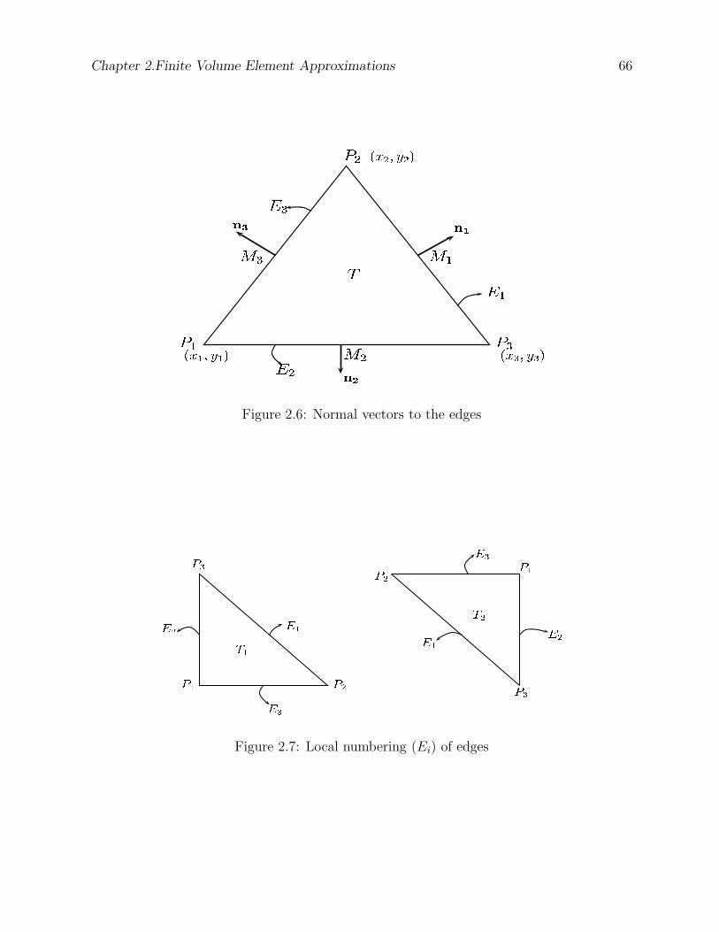
Chapter 2.Finite Volume Element Approximations 66
!
"$#
"&%"('
Figure 2.6: Normal vectors to the edges
)+* ),
)-
./,
),
)-
)0*
.1*
2&-
2&, 23*23* 2&,
2&-
Figure 2.7: Local numbering (Ei) of edges
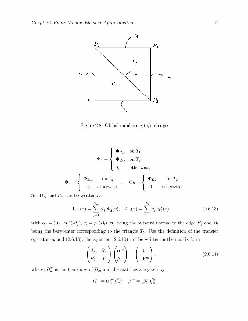
Chapter 2.Finite Volume Element Approximations 67
Figure 2.8: Global numbering (ei) of edges
,
Φ3 =
ΦE1, on T1
ΦE1, on T2
0, otherwise.
Φ4 =
ΦE2, on T2
0, otherwise., Φ5 =
ΦE3, on T2
0, otherwise.
So, Um and Pm can be written as
Um(x) =Nm∑
j=1
αmj Φj(x), Pm(x) =Nt∑
l=1
βml χ∗l (x) (2.6.13)
with αj = (uh · nj)(Mj), βl = ph(Bl), nj being the outward normal to the edge Ej and Bl
being the barycenter corresponding to the triangle Tl. Use the definition of the transfer
operator γh and (2.6.13), the equation (2.6.10) can be written in the matrix form
Am Bm
BTm 0
αm
βm
=
0
−Fm
, (2.6.14)
where, BTm is the transpose of Bm and the matrices are given by
αm = (αmj )Nm
j=1, βm = (βml )Nt
l=1
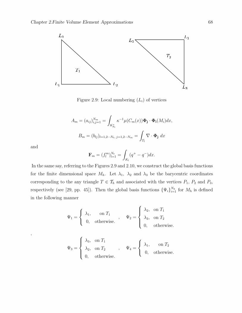
Chapter 2.Finite Volume Element Approximations 68
Figure 2.9: Local numbering (Li) of vertices
Am = (aij)Nm
i,j=1 =
∫
K∗pi
κ−1µ(Cm(x))Φj · Φi(Mi)dx,
Bm = (blj)l=1,2···Nt, j=1,2···Nm=
∫
Tl
∇ · Φj dx
and
Fm = (fml )Nt
l=1 =
∫
Kl
(q+ − q−)dx.
In the same say, referring to the Figures 2.9 and 2.10, we construct the global basis functions
for the finite dimensional space Mh. Let λ1, λ2 and λ3 be the barycentric coordinates
corresponding to the any triangle T ∈ Th and associated with the vertices P1, P2 and P3,
respectively (see [29, pp. 45]). Then the global basis functions ΨiNh
i=1 for Mh is defined
in the following manner
Ψ1 =
λ1, on T1
0, otherwise., Ψ2 =
λ2, on T1
λ3, on T2
0, otherwise.
,
Ψ3 =
λ3, on T1
λ2, on T2
0, otherwise.
, Ψ4 =
λ1, on T2
0, otherwise.
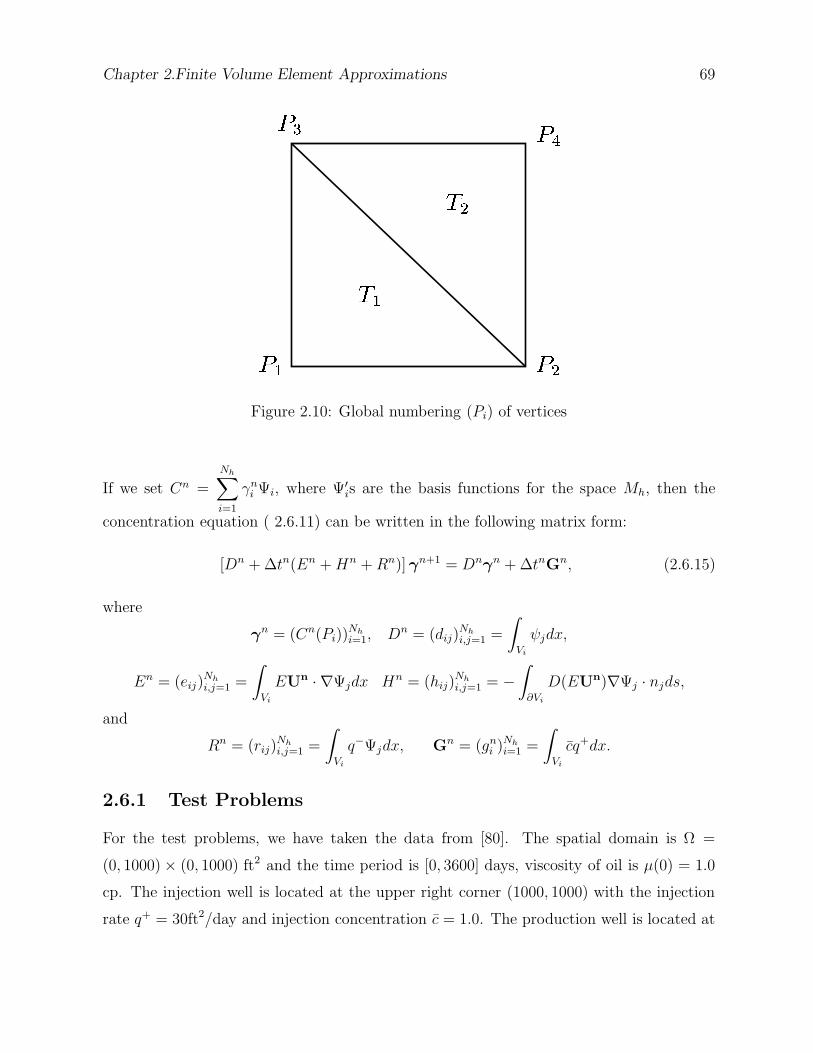
Chapter 2.Finite Volume Element Approximations 69
Figure 2.10: Global numbering (Pi) of vertices
If we set Cn =
Nh∑
i=1
γni Ψi, where Ψ′is are the basis functions for the space Mh, then the
concentration equation ( 2.6.11) can be written in the following matrix form:
[Dn + ∆tn(En +Hn +Rn)] γn+1 = Dnγn + ∆tnGn, (2.6.15)
where
γn = (Cn(Pi))Nh
i=1, Dn = (dij)Nh
i,j=1 =
∫
Vi
ψjdx,
En = (eij)Nh
i,j=1 =
∫
Vi
EUn · ∇Ψjdx Hn = (hij)Nh
i,j=1 = −∫
∂Vi
D(EUn)∇Ψj · njds,
and
Rn = (rij)Nh
i,j=1 =
∫
Vi
q−Ψjdx, Gn = (gni )Nh
i=1 =
∫
Vi
cq+dx.
2.6.1 Test Problems
For the test problems, we have taken the data from [80]. The spatial domain is Ω =
(0, 1000) × (0, 1000) ft2 and the time period is [0, 3600] days, viscosity of oil is µ(0) = 1.0
cp. The injection well is located at the upper right corner (1000, 1000) with the injection
rate q+ = 30ft2/day and injection concentration c = 1.0. The production well is located at
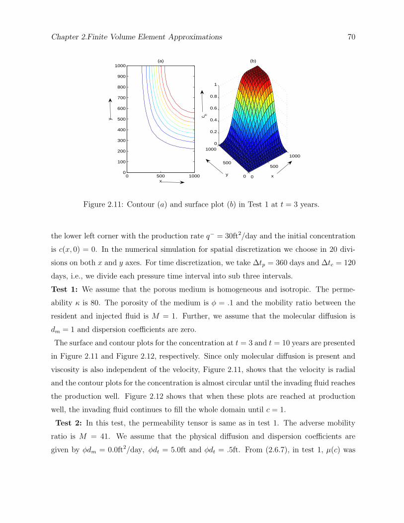
Chapter 2.Finite Volume Element Approximations 70
0
500
1000
0
500
10000
0.2
0.4
0.6
0.8
1
x
(b)
y
c h
x
y
(a)
0 500 10000
100
200
300
400
500
600
700
800
900
1000
Figure 2.11: Contour (a) and surface plot (b) in Test 1 at t = 3 years.
the lower left corner with the production rate q− = 30ft2/day and the initial concentration
is c(x, 0) = 0. In the numerical simulation for spatial discretization we choose in 20 divi-
sions on both x and y axes. For time discretization, we take ∆tp = 360 days and ∆tc = 120
days, i.e., we divide each pressure time interval into sub three intervals.
Test 1: We assume that the porous medium is homogeneous and isotropic. The perme-
ability κ is 80. The porosity of the medium is φ = .1 and the mobility ratio between the
resident and injected fluid is M = 1. Further, we assume that the molecular diffusion is
dm = 1 and dispersion coefficients are zero.
The surface and contour plots for the concentration at t = 3 and t = 10 years are presented
in Figure 2.11 and Figure 2.12, respectively. Since only molecular diffusion is present and
viscosity is also independent of the velocity, Figure 2.11, shows that the velocity is radial
and the contour plots for the concentration is almost circular until the invading fluid reaches
the production well. Figure 2.12 shows that when these plots are reached at production
well, the invading fluid continues to fill the whole domain until c = 1.
Test 2: In this test, the permeability tensor is same as in test 1. The adverse mobility
ratio is M = 41. We assume that the physical diffusion and dispersion coefficients are
given by φdm = 0.0ft2/day, φdt = 5.0ft and φdt = .5ft. From (2.6.7), in test 1, µ(c) was
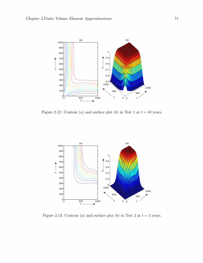
Chapter 2.Finite Volume Element Approximations 71
0
500
1000
0
500
10000.5
0.6
0.7
0.8
0.9
1
x
(b)
y
c hx
y
(a)
0 500 10000
100
200
300
400
500
600
700
800
900
1000
Figure 2.12: Contour (a) and surface plot (b) in Test 1 at t = 10 years.
0
500
1000
0
500
10000
0.2
0.4
0.6
0.8
1
x
(b)
y
c h
x
y
(a)
0 500 10000
100
200
300
400
500
600
700
800
900
1000
Figure 2.13: Contour (a) and surface plot (b) in Test 2 at t = 3 years.
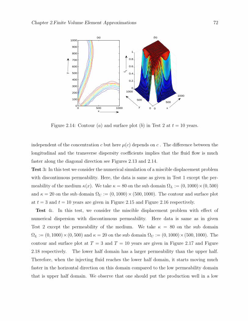
Chapter 2.Finite Volume Element Approximations 72
0
500
1000
0
500
10000
0.2
0.4
0.6
0.8
1
x
(b)
y
c h
x
y
(a)
0 500 10000
100
200
300
400
500
600
700
800
900
1000
Figure 2.14: Contour (a) and surface plot (b) in Test 2 at t = 10 years.
independent of the concentration c but here µ(c) depends on c . The difference between the
longitudinal and the transverse dispersity coefficients implies that the fluid flow is much
faster along the diagonal direction see Figures 2.13 and 2.14.
Test 3: In this test we consider the numerical simulation of a miscible displacement problem
with discontinuous permeability. Here, the data is same as given in Test 1 except the per-
meability of the medium κ(x). We take κ = 80 on the sub domain ΩL := (0, 1000)×(0, 500)
and κ = 20 on the sub domain ΩU := (0, 1000)× (500, 1000). The contour and surface plot
at t = 3 and t = 10 years are given in Figure 2.15 and Figure 2.16 respectively.
Test 4:. In this test, we consider the miscible displacement problem with effect of
numerical dispersion with discontinuous permeability. Here data is same as in given
Test 2 except the permeability of the medium. We take κ = 80 on the sub domain
ΩL := (0, 1000)×(0, 500) and κ = 20 on the sub domain ΩU := (0, 1000)×(500, 1000). The
contour and surface plot at T = 3 and T = 10 years are given in Figure 2.17 and Figure
2.18 respectively. The lower half domain has a larger permeability than the upper half.
Therefore, when the injecting fluid reaches the lower half domain, it starts moving much
faster in the horizontal direction on this domain compared to the low permeability domain
that is upper half domain. We observe that one should put the production well in a low

Chapter 2.Finite Volume Element Approximations 73
0
500
1000
0
500
10000
0.2
0.4
0.6
0.8
1
x
(b)
y
c h
x
y
(a)
0 500 10000
100
200
300
400
500
600
700
800
900
1000
Figure 2.15: Contour (a) and surface plot (b) in Test 3 at t = 3 years.
0
500
1000
0
500
10000.2
0.4
0.6
0.8
1
x
(b)
y
c h
x
y
(a)
0 500 10000
100
200
300
400
500
600
700
800
900
1000
Figure 2.16: Contour (a) and surface plot (b) in Test 3 at t = 10 years.
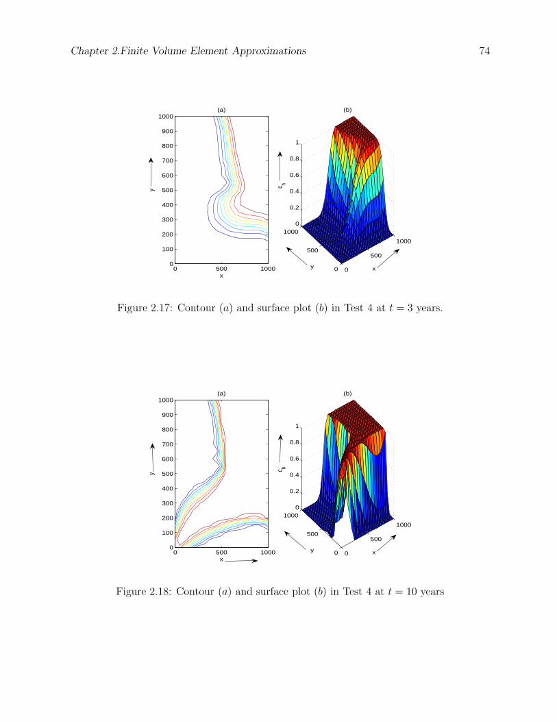
Chapter 2.Finite Volume Element Approximations 74
0
500
1000
0
500
10000
0.2
0.4
0.6
0.8
1
x
(b)
y
c h
x
y
(a)
0 500 10000
100
200
300
400
500
600
700
800
900
1000
Figure 2.17: Contour (a) and surface plot (b) in Test 4 at t = 3 years.
0
500
1000
0
500
10000
0.2
0.4
0.6
0.8
1
x
(b)
y
c h
x
y
(a)
0 500 10000
100
200
300
400
500
600
700
800
900
1000
Figure 2.18: Contour (a) and surface plot (b) in Test 4 at t = 10 years
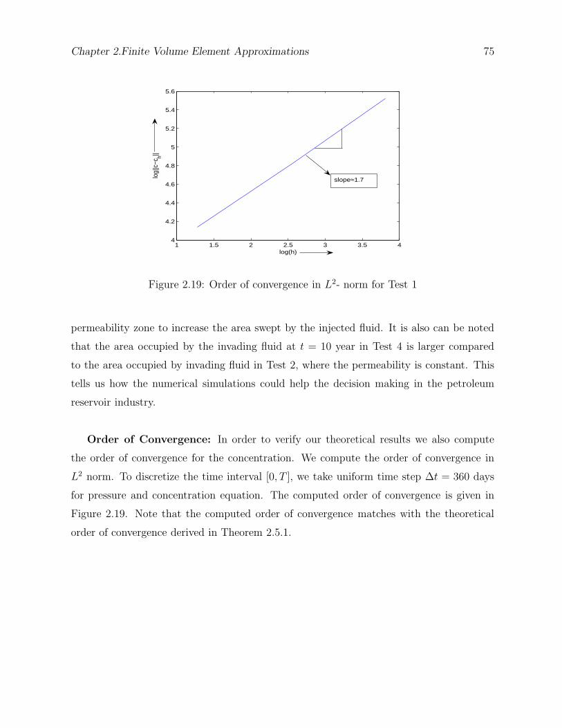
Chapter 2.Finite Volume Element Approximations 75
1 1.5 2 2.5 3 3.5 44
4.2
4.4
4.6
4.8
5
5.2
5.4
5.6
log(h)
log|
|c−c
h||
slope≈1.7
Figure 2.19: Order of convergence in L2- norm for Test 1
permeability zone to increase the area swept by the injected fluid. It is also can be noted
that the area occupied by the invading fluid at t = 10 year in Test 4 is larger compared
to the area occupied by invading fluid in Test 2, where the permeability is constant. This
tells us how the numerical simulations could help the decision making in the petroleum
reservoir industry.
Order of Convergence: In order to verify our theoretical results we also compute
the order of convergence for the concentration. We compute the order of convergence in
L2 norm. To discretize the time interval [0, T ], we take uniform time step ∆t = 360 days
for pressure and concentration equation. The computed order of convergence is given in
Figure 2.19. Note that the computed order of convergence matches with the theoretical
order of convergence derived in Theorem 2.5.1.
Chapter 3
Discontinuous Galerkin Finite
Volume Element Approximations
3.1 Introduction
The main objective in this chapter is to study a discontinuous finite volume element method
for the approximation of the concentration equation. As in Chapter 2, we have used a mixed
finite volume element method for the approximation of the pressure-velocity equation. A
priori error estimates in L∞(L2) norm are derived for velocity, pressure and concentration
for the semidiscrete and the fully discrete schemes. Numerical results are presented to
validate our theoretical results.
In recent years, there has been a renewed interest in Discontinuous Galerkin (DG) meth-
ods for the numerical approximation of partial differential equations. This is due to their
flexibility in local mesh adaptivity and handling nonuniform degrees of approximation for
solutions whose smoothness exhibit variation over the computational domain. DG methods
have the advantage that they are element-wise conservative and are easy to implement with
high degree of piecewise polynomials compared to other numerical methods such as con-
forming finite element methods, finite volume element methods, mixed finite element and
finite volume methods. In conforming finite element methods, the approximating functions
should satisfy some continuity criteria across the interelement boundaries, but in DG meth-
76
Chapter 3. Discontinuous Galerkin Finite Volume Element Approximations 77
ods, we have the freedom to choose discontinuous functions in the finite element spaces.
The first work on DG methods for elliptic and parabolic problems trace back to the
work by Douglas et al.[35] and Wheeler [82]. In 1973, Babuska [5] introduced a penalty
method to impose the Dirichlet boundary condition weakly. Interior Penalty (IP) methods
by Arnold [3] and Wheeler [82] arose from the observation that just as Dirichlet boundary
conditions, interelement continuity of approximating functions could be imposed weakly
instead of being built into the finite element space. This makes it possible to use spaces
of discontinuous piecewise polynomials of higher degree. These IP methods are based on
the Nitsche’s symmetric formulation and hence are presently called as symmetric interior
penalty Galerkin (SIPG) methods. The variational formulation of the SIPG methods is
symmetric and adjoint consistent. This helps in developing optimal L2- error estimates.
However, for the coercivity of the associated bilinear form, we need to choose the penalty
parameter large enough. Riviere et al. [70] and Houston et al. [50] have introduced and
analyzed the non-symmetric interior penalty Galerkin (NIPG) methods. A significant prop-
erty of NIPG method is that it is unconditionally stable with respect to the choice of the
penalty parameter. Hence, this advantage has stimulated renewed interest in applying these
methods to a large class of partial differential equations. It is noted that NIPG methods
are not adjoint consistent. In this case, optimal L2- error estimates can be derived by using
super-penalty techniques, for more details, we refer to [4].
Keeping in mind the advantages of FVEM and DG methods, it is natural to think of
discontinuous Galerkin finite volume element methods (DGFVEMs) for the numerical ap-
proximation of partial differential equations. In these methods, the support of the control
volumes are small compared to the standard FVM [60], mixed FVM [26]. Also the control
volumes have support inside the triangle in which they belong to and there is no contribu-
tion from adjacent triangles, see Figures 3.1 and 3.4. This property of the control volumes
makes DGFVEM more suitable for parallel computing. DGFVEM for the elliptic problems
has been discussed in [28, 55, 85] and for Stokes problem in [86].
As mentioned in Chapter 1, a mathematical model, which describes the miscible displace-
ment of one incompressible fluid over another in a porous medium is given by the following
set of partial differential equations.
Chapter 3. Discontinuous Galerkin Finite Volume Element Approximations 78
For a given T > 0, the pressure p and the concentration c satisfy
u = −κ(x)µ(c)
∇p ∀(x, t) ∈ Ω × J, (3.1.1)
∇ · u = q ∀(x, t) ∈ Ω × J, (3.1.2)
φ(x)∂c
∂t−∇ · (D(u)∇c− uc) = g(c) ∀(x, t) ∈ Ω × J, (3.1.3)
with boundary conditions
u · n = 0 ∀(x, t) ∈ ∂Ω × J, (3.1.4)
(D(u)∇c− uc) · n = 0 ∀(x, t) ∈ ∂Ω × J, (3.1.5)
and initial condition
c(x, 0) = c0(x) ∀x ∈ Ω, (3.1.6)
where g(c) = cq. Since the concentration equation (3.1.3) has the transport term u · ∇c,which dominates the diffusion term, the solution of (3.1.3) varies rapidly from one part of
the domain to the other. Standard Galerkin methods based on C0- piecewise-polynomials
for such problems show unacceptable oscillations in the approximation. A use of C1-
piecewise-polynomials smear the front excessively leading to very smooth approximations.
To strike a balance between these two methods, Douglas and Dupont [35] have introduced
and analyzed a new method which uses interior penalties across the interior edges of the
triangles for convection dominated diffusion equation. Wheeler et al. [83] have extended
this procedure for the approximation of convection dominated diffusion equation for in-
compressible miscible displacement problem in a porous media.
Sun et al. [76] applied the mixed FEM for pressure-velocity equation and discontinuous
Galerkin FEM for approximating the concentration. Further, Sun and Wheeler [77] ap-
plied symmetric and nonsymmetric discontinuous Galerkin methods for approximation of
the concentration equation by assuming that the velocity is known and time independent.
In this chapter, we apply mixed FVEM for the approximation of pressure-velocity equations
(3.1.1)-(3.1.2) and a discontinuous Galerkin FVEM for approximating the concentration
equation (3.1.3).
Chapter 3. Discontinuous Galerkin Finite Volume Element Approximations 79
This chapter is organized as follows. In Section 3.2, the weak formulation for incom-
pressible miscible displacement problems in a porous media is described. In Section 3.3, we
discuss the DGFVEM formulation. The existence and uniqueness of solution to the discrete
problem is also discussed. A priori error estimates for velocity, pressure and concentration
are presented in Section 3.4. Finally in Section 3.5, the numerical procedure is discussed
and the results of some numerical experiments are presented.
3.2 Weak formulation
Define
U = v ∈ H(div; Ω) : v · n = 0 on ∂Ω.
and
W = L2(Ω)/R.
Then, the weak form the pressure-velocity equations (2.1.1)-(2.1.2) is to seek
(u, p) : J −→ U ×W satisfying
(κ−1µ(c)u,v) − (∇ · v, p) = 0 ∀v ∈ U, (3.2.1)
(∇ · u, w) = (q, w) ∀w ∈ W. (3.2.2)
The concentration equation (3.1.3) can be put in the weak form as follows. Find a differ-
entiable map c : J −→ H1(Ω) such that
(φ∂c
∂t, z) + a(u; c, z) = (g(c), z) ∀z ∈ H1(Ω), (3.2.3)
c(x, 0) = c0(x) ∀x ∈ Ω,
where a(v; ·, ·) : H1(Ω) ×H1(Ω) −→ R is a continuous bilinear form defined by
a(v;φ, ψ) =
∫
Ω
(D(v)∇φ− vφ) · ∇ψ dx ∀φ, ψ ∈ H1(Ω),v ∈ R2.
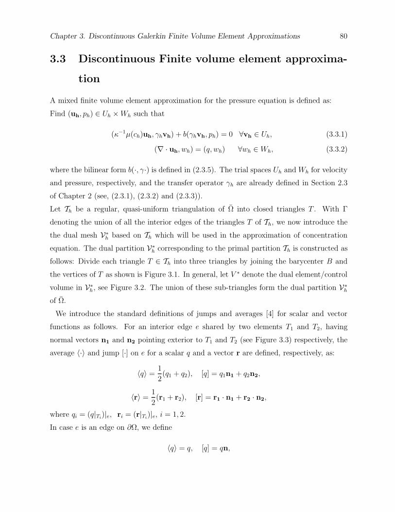
Chapter 3. Discontinuous Galerkin Finite Volume Element Approximations 80
3.3 Discontinuous Finite volume element approxima-
tion
A mixed finite volume element approximation for the pressure equation is defined as:
Find (uh, ph) ∈ Uh ×Wh such that
(κ−1µ(ch)uh, γhvh) + b(γhvh, ph) = 0 ∀vh ∈ Uh, (3.3.1)
(∇ · uh, wh) = (q, wh) ∀wh ∈ Wh, (3.3.2)
where the bilinear form b(·, γ·) is defined in (2.3.5). The trial spaces Uh and Wh for velocity
and pressure, respectively, and the transfer operator γh are already defined in Section 2.3
of Chapter 2 (see, (2.3.1), (2.3.2) and (2.3.3)).
Let Th be a regular, quasi-uniform triangulation of Ω into closed triangles T . With Γ
denoting the union of all the interior edges of the triangles T of Th, we now introduce the
the dual mesh V∗h based on Th which will be used in the approximation of concentration
equation. The dual partition V∗h corresponding to the primal partition Th is constructed as
follows: Divide each triangle T ∈ Th into three triangles by joining the barycenter B and
the vertices of T as shown is Figure 3.1. In general, let V ∗ denote the dual element/control
volume in V∗h, see Figure 3.2. The union of these sub-triangles form the dual partition V∗
h
of Ω.
We introduce the standard definitions of jumps and averages [4] for scalar and vector
functions as follows. For an interior edge e shared by two elements T1 and T2, having
normal vectors n1 and n2 pointing exterior to T1 and T2 (see Figure 3.3) respectively, the
average 〈·〉 and jump [·] on e for a scalar q and a vector r are defined, respectively, as:
〈q〉 =1
2(q1 + q2), [q] = q1n1 + q2n2,
〈r〉 =1
2(r1 + r2), [r] = r1 · n1 + r2 · n2,
where qi = (q|Ti)|e, ri = (r|Ti
)|e, i = 1, 2.
In case e is an edge on ∂Ω, we define
〈q〉 = q, [q] = qn,
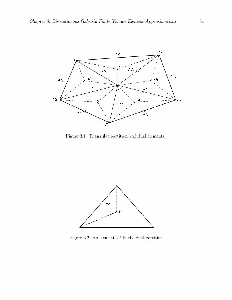
Chapter 3. Discontinuous Galerkin Finite Volume Element Approximations 81
Figure 3.1: Triangular partition and dual elements.
!
Figure 3.2: An element V ∗ in the dual partition.
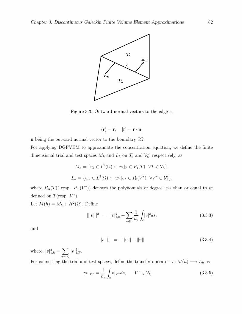
Chapter 3. Discontinuous Galerkin Finite Volume Element Approximations 82
Figure 3.3: Outward normal vectors to the edge e.
〈r〉 = r, [r] = r · n,
n being the outward normal vector to the boundary ∂Ω.
For applying DGFVEM to approximate the concentration equation, we define the finite
dimensional trial and test spaces Mh and Lh on Th and V∗h, respectively, as
Mh = vh ∈ L2(Ω) : vh|T ∈ P1(T ) ∀T ∈ Th,
Lh = wh ∈ L2(Ω) : wh|V ∗ ∈ P0(V∗) ∀V ∗ ∈ V∗
h,
where Pm(T )( resp. Pm(V ∗)) denotes the polynomials of degree less than or equal to m
defined on T (resp. V ∗).
Let M(h) = Mh +H2(Ω). Define
|||v|||2 = |v|21,h +∑
e∈Γ
1
he
∫
e
[v]2ds, (3.3.3)
and
‖|v‖|1 = ‖|v‖| + ‖v‖, (3.3.4)
where, |v|21,h =∑
T∈Th
|v|21,T .
For connecting the trial and test spaces, define the transfer operator γ : M(h) −→ Lh as
γv|V ∗ =1
he
∫
e
v|V ∗ds, V ∗ ∈ V∗h, (3.3.5)
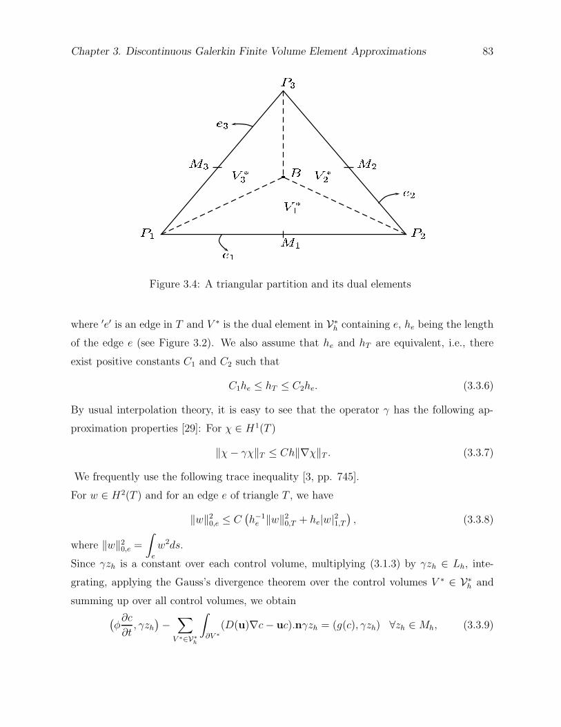
Chapter 3. Discontinuous Galerkin Finite Volume Element Approximations 83
Figure 3.4: A triangular partition and its dual elements
where ′e′ is an edge in T and V ∗ is the dual element in V∗h containing e, he being the length
of the edge e (see Figure 3.2). We also assume that he and hT are equivalent, i.e., there
exist positive constants C1 and C2 such that
C1he ≤ hT ≤ C2he. (3.3.6)
By usual interpolation theory, it is easy to see that the operator γ has the following ap-
proximation properties [29]: For χ ∈ H1(T )
‖χ− γχ‖T ≤ Ch‖∇χ‖T . (3.3.7)
We frequently use the following trace inequality [3, pp. 745].
For w ∈ H2(T ) and for an edge e of triangle T , we have
‖w‖20,e ≤ C
(
h−1e ‖w‖2
0,T + he|w|21,T)
, (3.3.8)
where ‖w‖20,e =
∫
e
w2ds.
Since γzh is a constant over each control volume, multiplying (3.1.3) by γzh ∈ Lh, inte-
grating, applying the Gauss’s divergence theorem over the control volumes V ∗ ∈ V∗h and
summing up over all control volumes, we obtain
(
φ∂c
∂t, γzh
)
−∑
V ∗∈V∗
h
∫
∂V ∗
(D(u)∇c− uc).nγzh = (g(c), γzh) ∀zh ∈Mh, (3.3.9)
Chapter 3. Discontinuous Galerkin Finite Volume Element Approximations 84
where n denotes the outward unit normal vector to the boundary ∂V ∗ of V ∗.
Let V ∗j ∈ V∗
h(j = 1, 2, 3) be the three triangles in T ∈ Th, (see Figure 3.4). Then,
∑
V ∗∈V∗
h
∫
∂V ∗
(D(u)∇c− uc) · nγzhds =∑
T∈Th
3∑
j=1
∫
∂V ∗
j
(D(u)∇c− uc) · nγzhds
=∑
T∈Th
3∑
j=1
∫
Pj+1BPj
(D(u)∇c− uc) · nγzhds+∑
T∈Th
∫
∂T
(D(u)∇c− uc) · nγzhds,(3.3.10)
where, P4 = P1, see Figure 3.4.
For any four real numbers a, b, c and d, we have
ac− bd =1
2(a + b)(c− d) +
1
2(a− b)(c + d). (3.3.11)
Since [(D(u)∇c− uc)] = 0 from (2.1.14), we have from (3.3.10) and (3.3.11)
∑
V ∗∈V∗
h
∫
∂V ∗
(D(u)∇c− uc) · nγzhds =∑
T∈Th
3∑
j=1
∫
Pj+1BPj
(D(u)∇c− uc) · nγzhds
+∑
e∈Γ
∫
e
[γzh] · 〈D(u)∇c− uc〉ds. (3.3.12)
For a fixed positive real number M , and v ∈ R2, define the following cut-off operator
vM = M(v)(x) = min (|v(x)|,M)v(x)
|v(x)| , (3.3.13)
Moreover, since later on we will assume that the Darcy velocity u ∈ (L∞(Ω))2, then M
can be chosen such that ‖u‖(L∞(Ω))2 ≤M and this implies that
uM = M(u) = u. (3.3.14)
It is easy to check that the “cut-off” operator M is uniformly Lipschitz continuous in the
following sense, (see [76, pp. 331]):
‖M(u) −M(v)‖(L∞(Ω))2 ≤ ‖u − v‖(L∞(Ω))2 . (3.3.15)
Proof of (3.3.15) is straightforward. Note that for a fixed x ∈ Ω, we have
|M(u) −M(v)|(x) ≤ |u − v|(x), (3.3.16)
Chapter 3. Discontinuous Galerkin Finite Volume Element Approximations 85
which can be shown by taking three cases (i) |u| ≤M, |v| ≤ M , (ii) |u| > M, |v| ≤M and
(iii) |u| > M, |v| > M and using the definition of M. Now take the essential supremum
on both sides of (3.3.16) the proof is completed.
By definition of M, it can be seen that
‖uMh ‖(L∞(Ω))2 ≤M. (3.3.17)
Now we are in a position to define the DG finite volume scheme for the concentration equa-
tion. The discontinuous Galerkin finite volume element scheme corresponding to (3.2.3) is
defined as:
Find ch(t) ∈Mh such that
(φ∂ch∂t
, γzh) + Ah(uMh ; ch, zh) = (g(ch), γzh) ∀zh ∈Mh, (3.3.18)
ch(0) = c0,h.
Here, uMh is the “cut-off” function of uh defined in (3.3.13) and c0,h be an approximation
to c0 to be defined later, the bilinear form Ah(v; ·, ·) : M(h) ×M(h) −→ R be defined by
Ah(v;φ, ψ) = A1(v;φ, ψ) −∑
e∈Γ
∫
e
[γψ] · 〈D(v)∇φ− vφ〉ds
−∑
e∈Γ
∫
e
[γφ] · 〈D(v)∇ψ〉ds+∑
e∈Γ
∫
e
α
he[φ] · [ψ]ds ∀v ∈ R
2, (3.3.19)
with A1(v;φ, ψ) = −∑
T∈Th
3∑
j=1
∫
Pj+1BPj
(
D(v)∇φ−vφ)
·n γψ ds and α is a penalty parameter
to be defined later. Note that (3.3.18) is consistent with (3.3.9). Now, based on the analysis
of [85], we prove the following two lemmas, which will be useful in proving the coercivity
and boundedness of the bilinear form Ah(u; ·, ·).
Lemma 3.3.1 The following result holds true: For χ, ψ ∈ M(h), we have
A1(u;χ, ψ) =∑
T∈Th
∫
T
(D(u)∇χ− uχ) · ∇ψ dx+∑
T∈Th
∫
∂T
(D(u)∇χ− uχ) · n)(γψ − ψ)ds
+∑
T∈Th
∫
T
∇ · (D(u)∇χ− uχ)(ψ − γψ)ds. (3.3.20)
Chapter 3. Discontinuous Galerkin Finite Volume Element Approximations 86
Proof. A use of Gauss divergence theorem on each on the control volume V ∗j , j = 1, 2, 3,
(see Figure 3.4), yields
A1(u;χ, ψ) = −∑
T∈Th
3∑
j=1
γψ
∫
Pj+1BPj
(D(u)∇χ− uχ) · n ds
=∑
T∈Th
3∑
j=1
γψ
∫
PjPj+1
(D(u)∇χ− uχ) · n ds−∑
T∈Th
3∑
j=1
∫
V ∗
j
γψ∇ · (D(u)∇χ− uχ)dx
=∑
T∈Th
∫
∂T
(γψ − ψ)(D(u)∇χ− uχ) · n ds+∑
T∈Th
∫
∂T
ψ(D(u)∇χ− uχ) · n ds
−∑
T∈Th
3∑
j=1
∫
V ∗
j
γψ∇ · (D(u)∇χ− uχ)dx
A use of Gauss’s divergence theorem once more yields,
A1(u;χ, ψ) =∑
T∈Th
∫
∂T
(γψ − ψ)(D(u)∇χ− uχ) · n ds+∑
T∈Th
∫
T
(D(u)∇χ− uχ) · ∇ψ dx
+∑
T∈Th
∫
T
∇ · (D(u)∇χ− uχ)ψ dx−∑
T∈Th
3∑
j=1
∫
V ∗
j
γψ∇ · (D(u)∇χ− uχ) dx
=∑
T∈Th
∫
∂T
(γψ − ψ)(D(u)∇χ− uχ) · n ds+∑
T∈Th
∫
T
(D(u)∇χ− uχ) · ∇ψ dx
+∑
T∈Th
∫
T
∇ · (D(u)∇χ− uχ)(ψ − γψ)dx.
This completes the proof.
Following the similar proof techniques, which we have used in Lemma 3.3.1. It is easy to
check that for χ, ψ ∈M(h), we have
A1(u;χ, ψ) =∑
T∈Th
∫
T
(D(u)∇χ) · ∇ψ dx+∑
T∈Th
∫
∂T
(D(u)∇χ) · n)(γψ − ψ)ds
+∑
T∈Th
∫
T
∇ · (D(u)∇χ)(ψ − γψ)ds, (3.3.21)
where
A1(u;χ, ψ) = −∑
T
3∑
j=1
∫
Pj+1BPj
(D(u)∇χ) · nγψ ds
.
Chapter 3. Discontinuous Galerkin Finite Volume Element Approximations 87
Lemma 3.3.2 If χh ∈Mh, then
A1(u;χh, χh) ≥ α0
∑
T∈Th
‖∇χh‖2 − C1h‖|χh‖|2 − C2‖χh‖2. (3.3.22)
Proof. Rewrite A1(u, χh, ψh) as
A1(u, χh, ψh) = −∑
T∈Th
3∑
j=1
∫
Pj+1BPj
(D(u)∇χh) · n γψh ds
+∑
T∈Th
3∑
j=1
∫
Pj+1BPj
u · nχh γψh ds. (3.3.23)
Using the same argument as in the proof of (2.3.37), it can be easily proved that
−∑
T∈Th
3∑
j=1
∫
Pj+1BPj
(D(u)∇χh) · nγχh ds ≥ α0
∑
T∈Th
‖∇χh‖2T − C1h‖|χh‖|2. (3.3.24)
Since γψh is constant on each control volume V ∗, set γψh|V ∗
l= ψl. Using the Cauchy-
Schwarz inequality and referring to Figure 3.4, we obtain
3∑
j=1
∫
Pj+1BPj
u · nχh γψh ds =3∑
l=1
∫
PlB
u · nlχh(ψl+1 − ψl)ds (ψ4 = ψ1)
≤3∑
l=1
|ψl+1 − ψl|∫
PlB
u · nl χh ds ≤ C3∑
l=1
|ψl+1 − ψl|∫
PlB
χh ds
A use of the trace inequality (3.3.8) yields
3∑
j=1
∫
Pj+1BPj
u · nχhγψh ds ≤ C3∑
l=1
|ψl+1 − ψl| ‖χh‖L2(PlB)(meas(PlB))1/2
≤ C3∑
l=1
|ψl+1 − ψl| ‖χh‖L2(PlB)h1/2T
≤ Ch1/2T
3∑
l=1
|ψl+1 − ψl|[
h−1/2T ‖χh‖T + h
1/2T ‖∇χh‖T
]
(3.3.25)
Now using Taylor series expansion and (2.3.18), we find that
|ψl+1 − ψl| ≤ hT
[
|∂ψh∂x
| + |∂ψh∂y
|]
≤[(
|∂ψh∂x
|2 + |∂ψh∂y
|2)
h2T
]1/2
≤ C|ψh|1,h,T , l = 1, 2, 3. (3.3.26)
Chapter 3. Discontinuous Galerkin Finite Volume Element Approximations 88
Substituting (3.3.26) in (3.3.25), we arrive at
3∑
j=1
∫
Pj+1BPj
u · nχh γψh ds ≤ C|ψh|1,h,T[
‖χh‖T + hT‖∇χh‖T]
. (3.3.27)
Taking summation over all the triangles T ∈ Th, we obtain
∑
T∈Th
3∑
j=1
∫
Pj+1BPj
u · nχh γψh ds ≤ C‖|ψh‖| (‖χh‖ + h‖|χh‖|) . (3.3.28)
Substituting (3.3.24) and (3.3.28) in (3.3.23) and using Young’s inequality, we complete
the rest of the proof.
Lemma 3.3.3 [3, pp. 744] There exists a positive constant C independent of mesh size h
such that
‖φ‖ ≤ C‖|φ‖| ∀φ ∈M(h). (3.3.29)
Lemma 3.3.4 [60] The following results hold true: ∀φh ∈Mh,
(i)
∫
T
(φh − γφh) dx = 0 ∀T ∈ Th (ii)
∫
e
(φh − γφh) ds = 0 ∀e ∈ Γ.
Proof. Using (3.3.5), we have
∫
T
(φh − γφh)dx =
∫
T
φh dx−3∑
i=1
∫
V ∗
i
γφh dx
=
∫
T
φh dx−3∑
i=1
γφh|V ∗
i|V ∗i |
=
∫
T
φh dx−3∑
i=1
1
hei
∫
ei
φh ds |V ∗i |
= 0.
Here |V ∗i | denotes the area of the control volume V ∗
i . In the last equality we have used
|V ∗i | =
|T |3, i = 1, 2, 3 and the quadrature formula (2.3.11). Now (ii) follows directly from
(3.3.5). This completes the proof.
Chapter 3. Discontinuous Galerkin Finite Volume Element Approximations 89
Let fT be the average value of f over the triangle T . The using Lemma 3.3.4, the Cauchy-
Schwarz inequality and (3.3.7), we find that
∫
T
f(ψh − γψh)dx =
∫
T
(f − fT )(ψh − γψh)dx
≤ ‖f − fT‖T‖ψh − γψh‖T ≤ Ch2‖∇f‖T‖∇ψh‖T . (3.3.30)
Next, we show that the bilinear form Ah(u; ·, ·) satisfies a Garding type inequality. Using
Cauchy-Schwarz inequality and the trace inequality (3.3.8), we arrive at
∑
e∈Γ
∫
e
[γφh] · 〈D(u)∇ψh〉ds ≤(
∑
e∈Γ
h−1e
∫
e
[γφh]2ds
)1/2(∑
e∈Γ
he
∫
e
〈D(u)∇ψh〉2ds)1/2
≤ C‖D(u)‖0,∞
(
∑
e∈Γ
[γφh]2e
)1/2(∑
T∈Th
|∇ψh|2T
)1/2
≤ C
(
∑
e∈Γ
[γφh]2e
)1/2
‖|ψh‖|,
where [γφh]e =1
he
∫
e
[φh]ds. Now using (3.3.5) and the Cauchy-Schwarz inequality, we
obtain
[γφh]2e =
(
1
he
∫
e
[φh]ds
)2
≤(
1
he
)2 ∫
e
[φh]2ds
∫
e
ds =
∫
e
1
he[φh]
2ds. (3.3.31)
This implies that
∑
e∈Γ
∫
e
[γφh] · 〈D(u)∇ψh〉ds ≤ C
(
∑
e∈Γ
1
he
∫
e
[φh]2ds
)1/2
‖|ψh‖|, (3.3.32)
and similarly,
∑
e∈Γ
∫
e
[γφh] · 〈(D(u)∇ψh − uψh〉ds ≤ C
(
∑
e∈Γ
1
he
∫
e
[φh]2ds
)1/2
(‖|ψh‖| + ‖ψh‖).(3.3.33)
Lemma 3.3.5 There exist positive constants C and C3 independent of h such that for α
large enough, h small enough and v ∈ (L∞(Ω))2,
Ah(v;φh, φh) ≥ C‖|φh‖|2 − C3‖φh‖2 ∀φh ∈Mh. (3.3.34)
Chapter 3. Discontinuous Galerkin Finite Volume Element Approximations 90
Proof. Use (3.3.29), (3.3.32), (3.3.33) and (3.3.22) to obtain
Ah(v;φh, φh) ≥ α0
∑
T∈Th
‖∇φh‖2 − C1h‖|φh‖|2 − C2‖φh‖2 − C‖|φh‖|(
∑
e∈Γ
1
he
∫
e
[φh]2ds
)1/2
+α∑
e∈Γ
1
he
∫
e
[φh]2ds.
A use of Young’s inequality yields
Ah(v;φh, φh) ≥ α0
∑
T∈Th
‖∇φh‖2 − C1h‖|φh‖|2 − C2‖φh‖2 − C2
2α0
(
∑
e∈Γ
1
he
∫
e
[φh]2ds
)
−α0
2‖|φh‖|2 + α
∑
e∈Γ
1
he
∫
e
[φh]2ds
≥ α0
2
∑
T∈Th
‖∇φh‖2 − C1h‖|φh‖|2 − C2‖φh‖2 +(
α− C2
2α0− α0
2
)
∑
e∈Γ
1
he
∫
e
[φh]2ds
≥ C(α)‖|φh‖|2 − C3‖φh‖2 − C1h‖|φh‖|2
≥ C‖|φh‖|2 − C3‖φh‖2,
where C(α) = min(
α0
2, α− C2
2α0− α0
2
)
and α0 is the lower bound for matrix D(v). Here we
have to choose the parameter α such that the term(
α− C2
2α0− α0
2
)
is positive and h small
enough such that C = C(α) − C1h > 0. This completes the proof.
Lemma 3.3.6 For φ, ψ ∈M(h), we have
|Ah(u;φ, ψ)| ≤ C
[
‖|φ‖| +(
∑
T∈Th
h2T |φ|2,T
)1/2
‖|ψ‖|
+
‖|ψ‖| +(
∑
T∈Th
h2T |ψ|2,T
)1/2
‖|φ‖|]
. (3.3.35)
Further if φh, ψh ∈Mh, then
|Ah(u;φh, ψh)| ≤ C‖|φh‖| ‖|ψh‖|. (3.3.36)
Chapter 3. Discontinuous Galerkin Finite Volume Element Approximations 91
Proof. Rewrite Ah(u;φ, ψ) = A1h(u;φ, ψ) + A2
h(u;φ, ψ),
where
A1h(u;φ, ψ) = −
∑
T∈Th
3∑
j=1
∫
Pj+1BPj
(
D(u)∇φ)
· nγψ ds−∑
e∈Γ
∫
e
[γψ].〈D(u)∇ψ〉ds
−∑
e∈Γ
∫
e
[γφ] · 〈D(u)∇ψ〉ds+∑
e∈Γ
∫
e
α
he[φh] · [ψ]ds, (3.3.37)
and
A2h(u;φ, ψ) =
∑
T∈Th
3∑
j=1
∫
Pj+1BPj
uφ · nγψ +∑
e∈Γ
∫
e
[γψ] · 〈uφ〉ds. (3.3.38)
To bound the first term of A1h(u;φ, ψ), we use (3.3.21 ) to obtain
∣
∣
∣
∑
T∈Th
3∑
j=1
∫
Pj+1BPj
(
D(u)∇φ)
· nγψ ds∣
∣
∣≤∣
∣
∣
∣
∣
∑
T∈Th
∫
T
D(u)∇φ · ∇ψ dx
∣
∣
∣
∣
∣
+
∣
∣
∣
∣
∣
∑
T∈Th
∫
∂T
(D(u)∇φ · n)(γψ − ψ)ds
∣
∣
∣
∣
∣
+
∣
∣
∣
∣
∣
∑
T∈Th
∫
T
∇ · (D(u)∇φ)(ψ − γψ)ds
∣
∣
∣
∣
∣
A use of the Cauchy-Schwarz inequality gives us
∣
∣
∣
∑
T∈Th
3∑
j=1
∫
Pj+1BPj
(
D(u)∇φ)
· nγψ ds∣
∣
∣≤ ‖D(u)‖0,∞
(
∑
T∈Th
|∇φ|2T
)1/2(∑
T∈Th
|∇ψ|2T
)1/2
+‖D(u)‖0,∞
(
∑
T∈Th
∫
∂T
|∂φ∂n
|2ds)1/2(
∑
T∈Th
∫
∂T
|ψ − γψ|2ds)1/2
+‖D(u)‖1,∞
(
∑
T∈Th
|φ|1,T‖ψ − γψ‖T)
+ ‖D(u)‖0,∞
(
∑
T∈Th
|φ|2,T‖ψ − γψ‖T)
.
Using the trace inequality (3.3.8), we find that
∣
∣
∣
∑
T∈Th
3∑
j
∫
Pj+1BPj
(
D(u)∇φ)
· nγψ ds∣
∣
∣≤ C
[
|φ|1,h|ψ|1,h +
(
∑
T∈Th
h−1T |∇φ|2T + hT |φ|22,T
)1/2
(
∑
T∈Th
h−1T |ψ − γψ|2T + hT |ψ − γψ|21,T
)1/2
+∑
T∈Th
hT (|φ|1,T + |φ|2,T ) |ψ|1,T]
.
Chapter 3. Discontinuous Galerkin Finite Volume Element Approximations 92
Now using (3.3.7), we obtain
∣
∣
∣
∑
T∈Th
3∑
j=1
∫
Pj+1BPj
(
D(u)∇φ)
· nγψ ds∣
∣
∣≤ C
[
|φ|1,h|ψ|1,h +
(
∑
T∈Th
|φ|21,T + h2T |φ|22,T
)1/2
(
∑
T∈Th
|ψ|1,T)1/2
+∑
T∈Th
hT (|φ|1,T + |φ|2,T ) |ψ|1,T]
≤ C
[
|φ|1,h|ψ|1,h +
(
∑
T∈Th
h2T |φ|22,T
)1/2
|ψ|1,h]
(3.3.39)
Following the proof techniques of (3.3.32), we arrive at
|∑
e∈Γ
∫
e
[γψ] · 〈D(u)∇φ〉ds| ≤ C
(
∑
e∈Γ
1
he
∫
e
[ψ]2ds
)1/2 [∑
T∈Th
(
|φ|21,T + h2T |φ|22,T
)
]1/2
, (3.3.40)
and
|∑
e∈Γ
∫
e
[γφ] · 〈D(u)∇ψ〉ds| ≤ C
(
∑
e∈Γ
1
he
∫
e
[φ]2ds
)1/2 [∑
T∈Th
(
|ψ|21,T + h2T |ψ|22,T
)
]1/2
. (3.3.41)
Note that
∣
∣
∣
∣
∣
∑
e∈Γ
1
he
∫
e
[φ] · [ψ]ds
∣
∣
∣
∣
∣
≤(
∑
e∈Γ
1
he
∫
e
[φ]2ds
)1/2(∑
e∈Γ
1
he
∫
e
[ψ]2ds
)1/2
. (3.3.42)
Using (3.3.39)-(3.3.42) in (3.3.37), we obtain
|A1h(u;φ, ψ)| ≤ C
[
|φ|1,h|ψ|1,h +
(
∑
e∈Γ
1
he
∫
e
[ψ]2ds
)1/2(∑
T∈Th
(
|φ|21,T + h2T |φ|22,T
)
)1/2
+
(
∑
e∈Γ
1
he
∫
e
[φ]2ds
)1/2(∑
T∈Th
(
|ψ|21,T + h2T |ψ|22,T
)
)1/2
+
(
∑
e∈Γ
1
he
∫
e
[φ]2ds
)1/2(∑
e∈Γ
1
he
∫
e
[ψ]2ds
)1/2 ]
.
Chapter 3. Discontinuous Galerkin Finite Volume Element Approximations 93
Using (3.3.3),
|A1h(u;φ, ψ)| ≤ C
[
|φ|1,h|ψ|1,h +
(
∑
e∈Γ
1
he
∫
e
[ψ]2ds
)1/2(∑
T∈Th
(
|φ|21,T + h2T |φ|22,T
)
)1/2
+|φ|1,h|ψ|1,h +
(
∑
e∈Γ
1
he
∫
e
[φ]2ds
)1/2(∑
T∈Th
(
|ψ|21,T + h2T |ψ|22,T
)
)1/2
+
(
∑
e∈Γ
1
he
∫
e
[φ]2ds
)1/2(∑
e∈Γ
1
he
∫
e
[ψ]2ds
)1/2 ]
≤ C
[
‖|φ‖| +(
∑
T∈Th
h2T |φ|22,T
)1/2
‖|ψ‖|
+
(‖|ψ‖| +(
∑
T∈Th
h2T |ψ|22,T
)1/2
‖|φ‖|]
.
Now we proceed to estimate the first term in A2h(u;φ, ψ). From (3.3.28), we have
∣
∣
∣
∣
∣
∑
T∈Th
3∑
j=1
∫
Pj+1BPj
u · n φ γψ ds
∣
∣
∣
∣
∣
≤ C ‖|ψ‖| (‖φ‖ + h‖|φ‖|) . (3.3.43)
Using (3.3.31) it can be easily seen that
∣
∣
∣
∣
∣
∑
e∈Γ
∫
e
[γψ] · 〈uφ〉ds∣
∣
∣
∣
∣
≤ C‖|ψ‖| ‖|φ‖|. (3.3.44)
Substitute (3.3.43) and (3.3.44) in (3.3.38), to obtain
|A2h(u;φ, ψ)| ≤ C (‖|φ‖| ‖|ψ‖| + ‖|φ‖| ‖ψ‖) . (3.3.45)
Combining the estimates derived for A1h(u;φ, ψ) and A2
h(u;φ, ψ) with (3.3.29), we complete
the proof of (3.3.35).
In particular, if φh ∈ Mh, then |φh|2,T = 0 and hence (3.3.36) directly follows from follows
from (3.3.35). This completes the proof.
Lemma 3.3.7 The operator γ has the following properties. For φh, ψh ∈Mh,
(φh, γψh) = (ψh, γφh). (3.3.46)
Chapter 3. Discontinuous Galerkin Finite Volume Element Approximations 94
Moreover, with ‖|φh‖|h = (φh, γφh) norms ‖| · ‖|h and ‖ · ‖ are equivalent, i.e., there exist
positive constants C1 and C2, independent of h such that
C1‖φh‖ ≤ ‖|φh‖|h ≤ C2‖φh‖ ∀φh ∈Mh, (3.3.47)
and
‖γφh‖ ≤ C‖φh‖ ∀φh ∈ Mh. (3.3.48)
Proof. Since
(φh, γψh) =∑
T∈Th
3∑
j=1
γψh|V ∗
j
∫
V ∗
j ∩T
φh dx,
using the definition of γ, we obtain
3∑
j=1
γψh|V ∗
j
∫
V ∗
j ∩T
φh dx = γψh|V ∗
1
∫
V ∗
1∩T
φh dx+ γψh|V ∗
2
∫
V ∗
2∩T
φh dx+ γψh|V ∗
3
∫
V ∗
3∩T
φh dx
=1
he1
∫
e1
ψh ds
∫
V ∗
1∩T
φh dx+1
he2
∫
e2
ψh ds
∫
V ∗
2∩T
φh dx
+1
he3
∫
e3
ψh ds
∫
V ∗
3∩T
φh dx.
Since ψh is linear on each triangle T , we use the following quadrature formula to compute
the edge integral
∫
ei
ψh ds =ψi + ψi+1
2for i = 1, 2, 3. (3.3.49)
Now a use of the quadrature formula (2.3.11) along with (3.3.49), yields
3∑
j=1
γψh|V ∗
j
∫
V ∗
j ∩T
φh dx =
(
ψ1 + ψ2
2
)
(φ1 + φ2 + φB)|V ∗
1 |3
+
(
ψ2 + ψ3
2
)
(φ2 + φ3 + φB)|V ∗
2 |3
+
(
ψ1 + ψ3
2
)
(φ1 + φ3 + φB)|V ∗
3 |3.
Chapter 3. Discontinuous Galerkin Finite Volume Element Approximations 95
Since φB =φ1 + φ2 + φ3
3, we have
3∑
j=1
γψh|V ∗
j
∫
V ∗
j ∩T
φh dx =|T |54
[
(ψ1 + ψ2)(4φ1 + 4φ2 + φ3) + (ψ2 + ψ3)(4φ2 + 4φ3 + φ1)
+(ψ3 + ψ1)(4φ3 + 4φ1 + φ2)]
=|T |54
[ψ1, ψ2, ψ3]
8 5 5
5 8 5
5 5 8
[φ1, φ2, φ3]T .
This prove that the inner product (·, γ·) is symmetric. To prove the equivalence of the
norms, rewrite
3∑
j=1
γφh|V ∗
j
∫
V ∗
j ∩T
φh dx =|T |54
[
8(φ21 + φ2
2 + φ23) + 10(φ1φ2 + φ2φ3 + φ1φ3)
]
=|T |54
[
3(φ21 + φ2
2 + φ23) + 5(φ1 + φ2 + φ3)
2]
. (3.3.50)
Since φh is linear on triangle T , we can use midpoint quadrature formula (2.3.12) to compute
the integral
∫
T
|φh|2 dx =|T |3
[
(
φ1 + φ2
2
)2
+
(
φ2 + φ3
2
)2
+
(
φ1 + φ3
2
)2]
=|T |12
[
φ21 + φ2
2 + φ23 + (φ1 + φ2 + φ3)
2]
. (3.3.51)
Equivalence of norms follow from (3.3.50) and (3.3.51). This completes the proof for
(3.3.47). To prove (3.3.48), note that
‖γφh‖2 =∑
T∈Th
3∑
j=1
∫
V ∗
j
|γφh|2dx.
Since γφh is constant over the control volumes, (γφh|V ∗
j= φj, say), we have
3∑
j=1
∫
V ∗
j
|γφh|2dx =
3∑
j=1
φ2j |V ∗
j | =
3∑
j=1
φ2j
|T |3. (3.3.52)
Now (3.3.48) follows from (3.3.52) and (3.3.51) and this completes the proof.
For a given ch, the existence and uniqueness of the discrete solution uh and ph can be shown
Chapter 3. Discontinuous Galerkin Finite Volume Element Approximations 96
in a similar way as in Chapter 2. Since uMh is the cut-off function of uh, the existence of
uh implies the existence of uMh . To show the existence and uniqueness of the concentration
in (3.3.18), we argue as follows. On substituting (uMh (ch)) in (3.3.18), we obtain a system
of nonlinear ordinary differential equations in ch. An appeal to Picard’s theorem yields the
existence of a unique solution in (0, th) for some 0 < th ≤ T . To continue the solution for
all t ∈ J , we need an a priori bound for ch.
Choosing zh = ch in (3.3.18) and using (3.3.46), we obtain
1
2
d
dt(φch, γch) + Ah(u
Mh ; ch, ch) ≤ |(g(ch), γch)| (3.3.53)
Using the Cauchy-Schwarz inequality and (3.3.48), we obtain
|(g(ch), γch)| ≤ C(
‖ch‖2 + ‖c‖2)
. (3.3.54)
Substituting (3.3.34) and (3.3.54) in (3.3.53), we arrive at
1
2
d
dt(φch, γch) + C2‖|ch‖|2 ≤ C3
(
‖ch‖2 + ‖c‖2)
. (3.3.55)
Integrating from 0 to T and using (3.3.47), we obtain
‖ch‖2 +
∫ T
0
‖|ch‖|2ds ≤ C
(
‖ch(0)‖2 +
∫ T
0
‖ch‖2ds+ +
∫ T
0
‖c‖2ds
)
(3.3.56)
A use of Gronwall’s lemma in (3.3.56) gives an a priori estimate in L2- norm for ch. Now
the a priori bound ‖ch‖L∞(L2) can be used to show the existence of a unique solution ch of
the concentration equation for all t ∈ J . This completes the part of unique solvability of
(3.3.1)-(3.3.2) and (3.3.18).
3.4 Error estimates
In this section, we discuss the error estimates for the semidiscrete scheme. The following
theorem which gives the estimates for velocity and pressure has been proved in Chapter 2
(see Theorem 2.4.1).
Chapter 3. Discontinuous Galerkin Finite Volume Element Approximations 97
Theorem 3.4.1 Assume that the triangulation Th is quasi-uniform. Let (u, p) and (uh, ph),
respectively, be the solutions of (3.2.1)-(3.2.2) and (3.3.1)-(3.3.2). Then, there exists a pos-
itive constant C independent of h, but dependent on the bounds of κ−1 and µ such that
‖u − uh‖(L2(Ω))2 + ‖p− ph‖ ≤ C[
‖c− ch‖ + h(‖u‖(H1(Ω))2 + ‖p‖1)]
, (3.4.1)
‖∇ · (u − uh)‖ ≤ Ch‖∇ · u‖1, (3.4.2)
provided u(t) ∈ (H1(Ω))2, ∇ · u(t) ∈ H1(Ω) and p(t) ∈ H1(Ω).
Then for finding the estimates for concentration, we split c − ch = (c − Rhc) + (Rhc −ch), where Rh is the Ritz projection to be defined below in (3.4.3). In Lemma 3.4.1 and
Lemma 3.4.3, we derive respectively H1 and L2- error estimates for Rh. Finally using these
estimates, we obtain a priori error estimates in L2- norm for the concentration.
3.4.1 Elliptic projection
Let Rh : H1(Ω) −→Mh be the projection of c defined by
B(u; c−Rhc, χh) = 0 ∀χh ∈Mh, (3.4.3)
where
B(u;ψ, χh) = Ah(u;ψ, χh) + (λψ, χh) ∀χh ∈Mh. (3.4.4)
Using the boundedness of Ah(u; ·, ·), we have
|B(u;ψ, χh)|
‖|ψ‖|1 +
(
∑
T∈Th
hT |ψ|22,T
)1/2
‖|χh‖|1 + ‖|χh‖|1‖|ψ‖|1
. (3.4.5)
Since Ah(u;χh, χh) ≥ C‖|χh‖|2 − C2‖χh‖2, if we choose λ such that λ − C2 ≥ 0. Then,
B(u;χh, χh) will be coercive in the norm ‖|·‖|1 defined in (3.3.4), i.e., there exists a positive
constant C independent of h such that
B(u;χh, χh) ≥ C‖|χh‖|21 ∀χh ∈Mh. (3.4.6)
Chapter 3. Discontinuous Galerkin Finite Volume Element Approximations 98
Below we discuss L2 and H1- a priori error bounds for c−Rhc.
Let Ihc ∈Mh be an interpolant of c, which has the following approximation properties [29]:
|c− Ihc|s,T ≤ Ch2−sT ‖c‖2,T ∀T ∈ Th, s = 0, 1, 2. (3.4.7)
Moreover, if φ ∈ W 2,∞(Ω), then
‖φ− Ihφ‖1,∞ ≤ Ch‖φ‖2,∞. (3.4.8)
Lemma 3.4.1 There exists a positive constant C independent of h such that
‖|c−Rhc‖|1 ≤ Ch‖c‖2, (3.4.9)
provided c ∈ H2(Ω).
Proof. Write c − Rhc = (c − Ihc) + (Ihc − Rhc), first we derive the bound for ‖|c− Ihc‖|.By the definition of ‖| · ‖|, we obtain
‖|c− Ihc‖|2 = |c− Ihc|21,h +∑
e∈Γ
1
he
∫
e
[c− Ihc]2ds (3.4.10)
Using the trace inequality (3.3.8) and (3.4.7), we find that
1
he
∫
e
[c− Ihc]2eds ≤ C
(
h−2e ‖c− Ihc‖2
0,T + |c− Ihc|21,T)
≤ Ch2T ‖c‖2
2,T (3.4.11)
Use (3.4.11), (3.4.10) and (3.4.7), to obtain
‖|c− Ihc‖|1 ≤ Ch‖c‖2. (3.4.12)
The coercivity (3.4.6) and boundedness (3.4.5) of bilinear form B(u; ·, ·) with (3.4.3) yields
‖|Ihc− Rhc‖|21 ≤ CB(u; Ihc− Rhc, Ihc− Rhc)
≤ CB(u; Ihc− c, Ihc− Rhc)
≤ C
[
‖|c− Ihc‖|1 +
(
∑
T∈Th
hT |c− Ihc|22,T
)1/2
‖|Rhc− Ihc‖|1
+‖|Rhc− Ihc‖|1‖|c− Ihc‖|1]
, (3.4.13)
Chapter 3. Discontinuous Galerkin Finite Volume Element Approximations 99
and hence,
‖|Ihc− Rhc‖|1 ≤ C‖|c− Ihc‖|1, (3.4.14)
where C depends on bound of D(u) given in (2.1.13). Combine the estimates of (3.4.12)
and (3.4.14) and use the triangle inequality to complete the proof.
Before going to the L2 error estimates, we introduce the following bilinear form
A(u; ·, ·) : M(h) ×M(h) −→ R which will be helpful in deriving optimal error estimate in
L2 norm.
A(u;φ, ψ) =∑
T∈Th
∫
T
(D(u)∇φ− uφ) · ∇ψ dx−∑
e∈Γ
∫
e
[ψ] · 〈D(u)∇φ− uφ〉ds
−∑
e∈Γ
∫
e
[φ] · 〈D(u)∇ψ〉ds+∑
e∈Γ
∫
e
α
he[φ] · [ψ]ds. (3.4.15)
For our further use, let us introduce the following error function
εa(u;ψ, χ) = A(u;ψ, χ) − Ah(u;ψ, χ) ∀χ ∈Mh. (3.4.16)
Below, we will prove a lemma which plays an important role in the proof of a priori L2
error estimates for the Ritz projection Rh.
Lemma 3.4.2 There exists a positive constant C such that
|εa(u, c−Rhc, φh)| ≤ Ch2(
‖g‖1 + |φ∂c∂t
|1 + ‖c‖2
+‖∇ · u‖1 + ‖u‖(H1(Ω))2
)
‖φh‖1 ∀φh ∈ Mh. (3.4.17)
Proof. From (3.4.15), we obtain
A(u; u− Rhc, φh) =∑
T∈Th
∫
T
(D(u)∇(c−Rhc) − u(c− Rhc)) · ∇φh dx
−∑
e∈Γ
∫
e
[φh] · 〈D(u)∇(c− Rhc) − u(c− Rhc)〉ds
−∑
e∈Γ
∫
e
[c− Rhc] · 〈D(u)∇φh〉ds
+∑
e∈Γ
∫
e
α
he[φh] · [c−Rhc]ds
= T1 + T2 + T3 +∑
e∈Γ
∫
e
α
he[φh] · [c−Rhc]ds, (3.4.18)
Chapter 3. Discontinuous Galerkin Finite Volume Element Approximations 100
Similarly, we find that
Ah(u; c− Rhc, φh) = −∑
T∈Th
3∑
j=1
∫
Pj+1BPj
((D(u)∇(c− Rhc) − u(c−Rhc)) · n) γφh ds
−∑
e∈Γ
∫
e
[γφh] · 〈D(u)∇(c− Rhc) − u(c−Rhc)〉ds
−∑
e∈Γ
∫
e
[γ(c−Rhc)] · 〈D(u)∇φh〉ds
+∑
e∈Γ
∫
e
α
he[φh] · [c− Rhc]ds
= Th1+ Th2
+ Th3+∑
e∈Γ
∫
e
α
he[φh] · [c− Rhc]ds. (3.4.19)
From (3.4.18) and (3.4.19), we arrive at
|A(u; c− Rhc, φh) − Ah(u; c−Rhc, φh)| ≤ |T1 − Th1| + |T2 − Th2
| + |T3 − Th3|. (3.4.20)
To estimate |T1 − Th1|, we use Lemma 3.3.1 to obtain
|T1 − Th1| ≤
∣
∣
∣
∣
∣
∑
T∈Th
∫
∂T
(φh − γφh)(
D(u)∇(c−Rhc)) − u(c− Rhc))
· n ds
∣
∣
∣
∣
∣
+
∣
∣
∣
∣
∣
∑
T∈Th
∫
T
∇ · (D(u)∇(c− Rhc) − u(c−Rhc))(φh − γφh)dx
∣
∣
∣
∣
∣
= |I1| + |I2|, say. (3.4.21)
To bound |I1| and |I2|, we follow the proof techniques given in [46]. Since ∇c·n is continuous
across the element boundaries, we find that
|I1| ≤∣
∣
∣
∣
∣
∑
T∈Th
∫
∂T
D(u)∇(c− Rhc) · n(φh − γφh)ds
∣
∣
∣
∣
∣
+
∣
∣
∣
∣
∣
∑
T∈Th
∫
∂T
u(c− Rhc) · n(φh − γφh)ds
∣
∣
∣
∣
∣
≤∣
∣
∣
∣
∣
∑
T∈Th
∫
∂T
(
(D − DT )∇(c− Rhc))
· n(φh − γφh)ds
∣
∣
∣
∣
∣
+‖c− Rhc‖∞
∣
∣
∣
∣
∣
∑
T∈Th
∫
∂T
u · n(φh − γφh)ds
∣
∣
∣
∣
∣
, (3.4.22)
Chapter 3. Discontinuous Galerkin Finite Volume Element Approximations 101
where D = D(u) and DT is a function designed in a piecewise manner such that for any
edge e of a triangle T ∈ Th,
DT (x) = D(xc), ∀x ∈ e,
and xc is the mid point of e. Since |DT − D| ≤ Ch‖D‖1,∞, we obtain from the Cauchy-
Schwarz inequality that
|I1| ≤ Ch‖D‖1,∞
∑
T∈Th
∫
∂T
|φh − γφh| |∇(c− Rhc) · n|ds
+‖c‖2
∣
∣
∣
∣
∣
∑
T∈Th
∫
∂T
(u − uT ) · n(φh − γφh)ds
∣
∣
∣
∣
∣
.
Using (3.3.7) and (3.4.9), we obtain
|I1| ≤ Ch[
(
∑
T∈Th
h−1T ‖φh − γφh‖2
T + hT |φh − γφh|21,T
)1/2
×(
∑
T∈Th
h−1T |c−Rhc|21,T + hT |c− Rhc|22,T
)1/2
+‖c‖2 h1/2T
(
∑
T∈Th
h−1T ‖φh − γφh‖2
T + hT |φh − γφh|21,T
)1/2
≤ Ch2‖φh‖1‖c‖2. (3.4.23)
|I2| can be bounded as follows:
|I2| ≤∣
∣
∣
∣
∣
∑
T∈Th
∫
T
∇ · (D(u)∇c− uc) −∇ · (D(u)∇Rhc)(φ− γφh)ds
∣
∣
∣
∣
∣
+
∣
∣
∣
∣
∣
∑
T∈Th
∫
T
∇ · (uRhc)(φ− γφh)ds
∣
∣
∣
∣
∣
.
Using (3.1.3), we obtain
I2 ≤∣
∣
∣
∣
∣
∑
T∈Th
∫
T
(
g − φ∂c
∂t−∇ · (D(u)∇Rhc)
)
(φ− γφh)ds
∣
∣
∣
∣
∣
+
∣
∣
∣
∣
∣
∑
T∈Th
∫
T
(∇ · u Rhc+ u · ∇Rhc)(φ− γφh)ds
∣
∣
∣
∣
∣
Chapter 3. Discontinuous Galerkin Finite Volume Element Approximations 102
A use of (3.3.30) and (3.3.7) yields
|I2| ≤ Ch2
(
‖g‖1 + ‖φ∂c∂t
‖1 + ‖c‖2 + ‖∇ · u‖1 + ‖u‖(H1(Ω))2
)
‖φh‖1. (3.4.24)
Combining (3.4.23), (3.4.24) and (3.4.21), we obtain the following bound for |T1 − Th1|.
|T1 − Th1| ≤ Ch2
(
‖g‖1 + ‖φ∂c∂t
‖1 + ‖c‖2 + ‖∇ · u‖1 + ‖u‖(H1(Ω))2
)
‖φh‖1. (3.4.25)
To obtain an estimate for T2 − Th2, we note that
|T2 − Th2| ≤
∣
∣
∣
∣
∣
∑
e∈Γ
∫
e
[φh − γφh] · 〈D(u)∇(c− Rhc)〉ds∣
∣
∣
∣
∣
+
∣
∣
∣
∣
∣
∑
e∈Γ
∫
e
[φh − γφh] · 〈u(c−Rhc)〉ds∣
∣
∣
∣
∣
= |J1| + |J2|, say. (3.4.26)
Using the same argument as in I1, we bound J1 as
|J1| =
∣
∣
∣
∣
∣
∑
e∈Γ
∫
e
[φh − γφh] · 〈D(u)∇(c− Rhc)〉ds∣
∣
∣
∣
∣
=
∣
∣
∣
∣
∣
∑
e∈Γ
∫
e
[φh − γφh] · 〈(D − DT )∇(c−Rhc)〉ds∣
∣
∣
∣
∣
.
Using the Cauchy-Schwarz inequality and the trace inequality (3.3.8), (3.3.7) and (3.4.9),
we find that
|J1| ≤ Ch‖D‖1,∞
∑
e∈Γ
∫
e
|[φh − γφh]| |〈∇(c−Rhc)〉|ds
≤ Ch
(
∑
T∈Th
h−1T ‖φh − γφh‖2
T + hT |φh − γφh|21,T
)1/2
×(
∑
T∈Th
h−1T |c− Rhc|21,T + hT |c−Rhc|22,T
)1/2
≤ Ch
(
∑
T∈Th
hT |φh|21,T
)1/2(∑
T∈Th
hT |c|22,T
)1/2
≤ Ch2‖φh‖1‖c‖2. (3.4.27)
Chapter 3. Discontinuous Galerkin Finite Volume Element Approximations 103
Similarly, we bound J2 as
|J2| =
∣
∣
∣
∣
∣
∑
e∈Γ
∫
e
[φh − γφh] · 〈u(c− Rhc)〉ds∣
∣
∣
∣
∣
≤ ‖c‖2
∣
∣
∣
∣
∣
∑
e∈Γ
∫
e
[φh − γφh] · 〈u − uT 〉ds∣
∣
∣
∣
∣
≤ Ch‖c‖2‖u‖(W∞
1(Ω))2
∑
e∈Γ
∫
e
[φh − γφh]ds
≤ Ch2‖c‖2‖φh‖1. (3.4.28)
Substituting (3.4.27) and (3.4.28) in (3.4.26), we obtain
|T2 − Th2| ≤ Ch2‖φh‖1‖c‖2. (3.4.29)
In order to estimate T3 − Th3, we rewrite it as
|T3 − Th3| =
∣
∣
∣
∣
∣
∑
e∈Γ
∫
e
[(c−Rhc) − γ(c− Rhc)] · 〈D(u)∇φh〉ds∣
∣
∣
∣
∣
=
∣
∣
∣
∣
∣
∑
e∈Γ
∫
e
[(c−Rhc) − γ(c− Rhc)] · 〈(D − DT )∇φh〉ds∣
∣
∣
∣
∣
,
and using the same arguments as in |I1|, we arrive at
|T3 − Th3| ≤ Ch‖D‖1,∞
∑
e∈Γ
∫
e
|[(c−Rhc) − γ(c− Rhc)]| |〈∇φh〉|ds
≤ Ch
(
∑
T∈Th
h−1T ‖(c− Rhc) − γ(c− Rhc)‖2
T + hT |(c− Rhc) − γ(c− Rhc)|21,T
)1/2
(
∑
T∈Th
h−1T ‖φh‖2
1,T
)1/2
≤ Ch
(
∑
T∈Th
hT |c− Rhc|21,T
)1/2(∑
T∈Th
h−1T ‖φh‖2
1,T
)1/2
≤ Ch
(
∑
T∈Th
h2T |c|22,T
)1/2(∑
T∈Th
‖φh‖21,T
)1/2
≤ Ch2‖c‖2‖φh‖1. (3.4.30)
Chapter 3. Discontinuous Galerkin Finite Volume Element Approximations 104
Now substitute (3.4.25), (3.4.29) and (3.4.30) in (3.4.20) to complete the rest of the proof.
Lemma 3.4.3 There exists a positive constant C independent of h such that
‖c− Rhc‖ ≤ Ch2
(
‖c‖2 + ‖g‖1 + ‖φ∂c∂t
‖1 + ‖∇ · u‖1 + ‖u‖(H1(Ω))2
)
. (3.4.31)
Proof. To obtain an optimal L2 estimate for c − Rhc, we now appeal to Aubin-Nitsche
duality argument. Let ψ ∈ H2(Ω) be a solution of the following adjoint problem
−∇ · (D(u)∇ψ) − u · ∇ψ + λψ = c− Rhc in Ω, (3.4.32)
D(u)∇ψ · n = 0 on ∂Ω,
satisfying the following elliptic regularity condition:
‖ψ‖2 ≤ C‖c− Rhc‖. (3.4.33)
Multiply the first equation (3.4.32) by c − Rhc and integrate over Ω. Then using (3.4.16)
and (3.4.3), we arrive at
‖c− Rhc‖2 = A(u; c− Rhc, ψ) + λ(ψ, c−Rhc)
=[
A(u; c− Rhc, ψ − ψh) + λ(c− Rhc, ψ − ψh)]
+εa(u; c− Rhc, ψh) = I1 + I2, say. (3.4.34)
For I1, use (3.4.9) to obtain
|I1| = |A(u; c− Rhc, ψ − ψh) + (u · ∇(c−Rhc), ψ − ψh) + λ(c− Rhc, ψ − ψh)|
≤ C
[
‖|c− Rhc‖|1 +
(
∑
T∈Th
hT |c− Rhc|22,T
)1/2
‖|ψ − ψh‖|1
+‖|ψ − ψh‖|1‖|c− Rhc‖|1]
≤ Ch‖c‖2‖|ψ − ψh‖|1. (3.4.35)
The following bound for I2 follows from Lemma 3.4.2.
|I2| ≤ Ch2
(
‖g‖1 + ‖φ∂c∂t
‖1 + ‖c‖2 + ‖∇ · u‖1 + ‖u‖(H1(Ω))2
)
‖ψh‖1. (3.4.36)
Chapter 3. Discontinuous Galerkin Finite Volume Element Approximations 105
Substitute (3.4.35) and (3.4.36) in (3.4.34) to find that
‖c− Rhc‖2 ≤ C
[
h‖c‖2‖ψ − ψh‖1 + h2(
‖g‖1 + ‖φ∂c∂t
‖1 + ‖c‖2
+‖∇ · u‖1 + ‖u‖(H1(Ω))2
)
‖ψh‖1
]
. (3.4.37)
Now choose ψh = Ihψ in (3.4.37) and use (3.4.33) with (3.4.7) to obtain
‖c− Rhc‖ ≤ Ch2
(
‖c‖2 + ‖g‖1 + ‖φ∂c∂t
‖1 + ‖∇ · u‖1 + ‖u‖(H1(Ω))2
)
,
and this completes the proof.
For finding a bound for ‖Rhc‖1,∞, we use (2.3.14), (3.4.8) (3.4.9) and (3.4.14)
‖Rhc‖1,∞ = ‖c−Rhc‖1,∞ + ‖c‖1,∞
= ‖c− Ihc‖1,∞ + ‖Ihc−Rhc‖1,∞ + ‖c‖1,∞
≤ C(
‖c− Ihc‖1,∞ + h−1‖Ihc− Rhc‖1 + ‖c‖1,∞
)
≤ C‖c‖2,∞. (3.4.38)
Lemma 3.4.4 There exists a positive constant C such that
|Ah(uM ;Rhc, θ) − Ah(uMh ;Rhc, θ)| ≤ C
(
‖u − uh‖(L2(Ω))2 + h‖∇ · (u − uh)‖
+‖|ρ‖|)
‖|θ‖| ∀θ ∈Mh. (3.4.39)
Proof: Using the definition of Ah(·; ·, ·), we obtain
|Ah(uM ;Rhc, θ) − Ah(uMh ;Rhc, θ)| =
∣
∣
∣
∣
∣
∑
T∈Th
3∑
j=1
∫
Pj+1BPj
(D(uM) −D(uMh ))∇Rhc · nγθ ds∣
∣
∣
∣
∣
+
∣
∣
∣
∣
∣
∑
e∈Γ
∫
e
[γRhc] · 〈(D(uM) −D(uMh ))∇θ〉 ds∣
∣
∣
∣
∣
+
∣
∣
∣
∣
∣
∑
e∈Γ
∫
e
[γθ] · 〈(D(uM) −D(uMh ))∇Rhc〉 ds∣
∣
∣
∣
∣
+
∣
∣
∣
∣
∣
∑
T∈Th
3∑
j=1
∫
Pj+1BPj
(uM − uMh )Rhc · n γθ ds
∣
∣
∣
∣
∣
+
∣
∣
∣
∣
∣
∑
e∈Γ
∫
e
[γθ] · 〈(uM − uMh )Rhc〉ds∣
∣
∣
∣
∣
= A1 + A2 + A3 + A4 + A5, say.
Chapter 3. Discontinuous Galerkin Finite Volume Element Approximations 106
To estimate A1, we note that
A1 =
∣
∣
∣
∣
∣
∑
T∈Th
3∑
j=1
∫
Pj+1BPj
(D(uM) −D(uMh ))∇Rhc · n γθ ds
∣
∣
∣
∣
∣
= |∑
T∈Th
KT |,
where KT =
3∑
j=1
∫
Pj+1BPj
(D(uM) −D(uMh ))∇Rhc · n γθ ds. Since γθ is constant over each
control volume V ∗, set γθ|V ∗
l= θl. Referring to Figure 3.4, KT can be written as follows:
KT =
3∑
l=1
∫
PlB
(D(uM) −D(uMh ))∇Rhc · nl(θl+1 − θl)ds (θ4 = θ1)
Then using (3.4.38) and the Cauchy-Schwarz, we obtain
KT ≤3∑
l=1
|θl+1 − θl|∫
PlB
|(D(uM) −D(uMh ))∇Rhc · nl|ds
≤ C3∑
l=1
|θl+1 − θl| ‖D(uM) −D(uMh )‖(L2(PlB))2×2 (meas(PlB))1/2 .
Apply Lemma 2.3.5, trace inequality (3.3.8) and (3.3.15) to obtain
KT ≤ C
3∑
l=1
|θl+1 − θl| ‖uM − uMh ‖(L2(PlB))2h1/2T
≤ C
3∑
l=1
|θl+1 − θl| ‖u − uh‖(L2(PlB))2h1/2T
≤ Ch1/2T
3∑
l=1
|θl+1 − θl|[
h−1/2T ‖u − uh‖T + h
1/2T ‖∇ · (u − uh)‖T
]
. (3.4.40)
Now using Taylor series expansion and (2.3.18), we obtain
|θl+1 − θl| ≤ hT
[
|∂θ∂x
| + |∂θ∂y
|]
≤[(
|∂θ∂x
|2 + |∂θ∂y
|2)
h2T
]1/2
≤ C|θ|1,h,T , l = 1, 2, 3. (3.4.41)
Substitute (3.4.41) in (3.4.40) to arrive at
KT ≤ C|θ|1,h,T (‖u − uh‖T + hT‖∇ · (u − uh)‖T ) .
Chapter 3. Discontinuous Galerkin Finite Volume Element Approximations 107
With the estimates of KT and Lemma 2.3.1, we obtain
A1 ≤ C(
‖u − uh‖(L2(Ω))2 + h‖∇ · (u − uh)‖)
‖|θ‖|. (3.4.42)
Since [γc] = 0, we can write
A2 =
∣
∣
∣
∣
∣
∑
e∈Γ
∫
e
[γRhc] · 〈(D(uM) −D(uMh ))∇θ〉 ds∣
∣
∣
∣
∣
=
∣
∣
∣
∣
∣
∑
e∈Γ
∫
e
[γRhc− γc] · 〈(D(uM) −D(uMh ))∇θ〉 ds∣
∣
∣
∣
∣
≤∣
∣
∣
∣
∣
∑
e∈Γ
∫
e
[γρ] · 〈D(uM)∇θ〉ds∣
∣
∣
∣
∣
+
∣
∣
∣
∣
∣
∑
e∈Γ
∫
e
[γρ] · 〈D(uMh )∇θ〉ds∣
∣
∣
∣
∣
. (3.4.43)
Using the same argument as in deriving (3.3.32), we obtain∣
∣
∣
∣
∣
∑
e∈Γ
∫
e
[γρ] · 〈D(uM)∇θ〉ds∣
∣
∣
∣
∣
≤ C‖|ρ‖| ‖|θ‖|, (3.4.44)
and similarly,∣
∣
∣
∣
∣
∑
e∈Γ
∫
e
[γρ] · 〈D(uMh )∇θ〉ds∣
∣
∣
∣
∣
≤ C‖|ρ‖| ‖|θ‖|. (3.4.45)
Substituting (3.4.44) and (3.4.45) in (3.4.43), we obtain
A2 ≤ C‖|ρ‖| ‖|θ‖|. (3.4.46)
Now, we bound A3 as follows: Using (3.4.38) and the Cauchy-Schwarz inequality, we obtain
A3 =
∣
∣
∣
∣
∣
∑
e∈Γ
∫
e
[γθ] · 〈(D(uM) −D(uMh ))∇Rhc〉ds∣
∣
∣
∣
∣
≤ ‖∇Rhc‖∞
∣
∣
∣
∣
∣
∑
e∈Γ
∫
e
[γθ] · 〈D(uM) −D(uMh )〉ds∣
∣
∣
∣
∣
≤ C
(
∑
e∈Γ
∫
e
[γθ]2ds
)1/2(∑
e∈Γ
‖D(uM) −D(uMh )‖2(L2(e))2×2
)1/2
.
Now using Lemma Lemma 2.3.5 and (3.3.15), we arrive at
A3 ≤ C
(
∑
e∈Γ
∫
e
[γθ]2ds
)1/2(∑
e∈Γ
‖uM − uMh ‖2(L2(e))2
)1/2
≤ C
(
∑
e∈Γ
∫
e
[γθ]2ds
)1/2(∑
e∈Γ
‖u − uh‖2(L2(e))2
)1/2
Chapter 3. Discontinuous Galerkin Finite Volume Element Approximations 108
Using the trace inequality (3.3.8), we obtain
A3 ≤ C‖|θ‖|(
‖u − uh‖(L2(Ω))2 + h‖∇ · (u − uh)‖)
. (3.4.47)
A4 can be bound in a similar way as A1:
A4 ≤ C‖|θ‖|(
‖u − uh‖(L2(Ω))2 + h‖∇ · (u − uh)‖)
. (3.4.48)
To bound A5, we use the same arguments used in A3 to obtain
A5 ≤ C‖|θ‖| (‖u − uh‖ + h‖∇ · (u − uh)‖) (3.4.49)
Combine the estimates derived for A1 · · ·A5 to complete the rest of the proof.
3.4.2 L∞(L2) estimates for concentration
In this subsection, we discuss an L∞(L2) norm error estimate for the concentration.
Theorem 3.4.2 Let c and ch be the solutions of (3.2.3) and (3.3.18), respectively, and let
ch(0) = c0,h = Rhc(0). Then, for sufficiently small h, there exists a positive constant C(T )
independent of h but dependent on the bounds of κ−1 and µ such that
‖c− ch‖2L∞(J ;L2) ≤ C(T )
[
∫ T
0
(
h4(‖g‖21 + ‖φ∂c
∂t‖2
1 + ‖u‖(H1(Ω))2 + ‖∇ · u‖1
+‖ct‖22 + ‖gt‖2
1 + ‖ut‖(H1(Ω))2 + ‖∇ · ut‖1 + ‖φ∂2c
∂t2‖2
1
+h2(‖c‖22 + ‖u‖2
(H1(Ω))2 + ‖p‖21))
ds
]
. (3.4.50)
Proof: Write c− ch = (c−Rhc) + (Rhc− ch) = ρ+ θ. Since the estimates of ρ are known,
we need to find only the estimates of θ.
Multiply (3.1.3) by γzh, integrate over Ω. Then subtract the resulting equation from
(3.3.18) to obtain
(
φ∂θ
∂t, γzh
)
+ Ah(uM ; c, zh) − Ah(u
Mh ; ch, zh) = −
(
φ∂ρ
∂t, γzh
)
+(g(c) − g(ch), γzh) ∀zh ∈Mh. (3.4.51)
Chapter 3. Discontinuous Galerkin Finite Volume Element Approximations 109
Put zh = θ and use the definition of Rh to obtain(
φ∂θ
∂t, γθ
)
+ Ah(uMh ; θ, θ) = −
(
φ∂ρ
∂t, γθ
)
+ (λρ, θ) +(
g(c) − g(ch), γθ)
−[
Ah(uM ;Rhc, θ) − Ah(u
Mh ;Rhc, θ)
]
= I1 + I2 + I3 + I4, say. (3.4.52)
Now we estimate Ij, j = 1, 2, 3, 4 one by one. To estimate I1, we use the Cauchy Schwartz
inequality, boundedness of φ and (3.3.48) to obtain
|I1| = |(
φ∂ρ
∂t, γθ
)
| ≤ C‖∂ρ∂t
‖ ‖θ‖. (3.4.53)
Similarly,
|I2| = |(λρ, θ)| ≤ C‖ρ‖ ‖θ‖. (3.4.54)
Using (2.1.7) and (3.3.48), I3 can be estimated as
|I3| ≤ |(g(ch) − g(c), γθ)| ≤ C‖c− ch‖ ‖θ‖. (3.4.55)
The bound for I4 follows from Lemma 3.4.4 and hence,
|I4| ≤ C(
‖u − uh‖(L2(Ω))2 + h‖∇ · (u − uh)‖ + ‖|ρ‖|)
‖|θ‖|. (3.4.56)
Substitute the estimates of I1, · · · , I4 in (3.4.52) and use (3.3.34), Young’s inequality, non
singularity of the function φ with standard kick back arguments to obtain
d
dt‖|θ‖|2h + (α0 − ε)‖|θ‖|2 ≤ C
[
h2‖∇ · (u − uh)‖2 + ‖|ρ‖|2‖u − uh‖2(L2(Ω))2
+‖c− ch‖2 + ‖ρ‖2 + ‖∂ρ∂t
‖2 + ‖θ‖2]
. (3.4.57)
Now, from (3.4.1),
‖u − uh‖(L2(Ω))2 ≤ C(
‖ρ‖ + ‖θ‖ + h(‖u‖(H1(Ω))2 + ‖p‖1))
. (3.4.58)
A use of (3.4.31), (3.4.58) and (3.4.2) in (3.4.57) yields
d
dt‖|θ‖|2h + α1‖|θ‖|2 ≤ C
[
h4(
‖g‖21 + ‖u‖(H1(Ω))2 + ‖∇ · u‖1 + ‖φ∂c
∂t‖2
1
+‖ct‖22 + ‖gt‖2
1 + ‖ut‖(H1(Ω))2 + ‖∇ · ut‖1 + ‖φ∂2c
∂t2‖2
1
)
+h2(‖c‖22 + ‖u‖2
(H1(Ω))2 + ‖p‖21) + ‖θ‖2
]
. (3.4.59)
Chapter 3. Discontinuous Galerkin Finite Volume Element Approximations 110
Since ch(0) = Rhc(0), this implies that θ(0) = 0. An application of Gronwall’s inequality
with (3.3.47), (3.4.59) yields
‖θ‖2L∞(J ;L2) ≤ C(T )
[
∫ T
0
h4(
‖g‖21 + ‖u‖(H1(Ω))2 + ‖∇ · u‖1
+‖φ∂c∂t
‖21 + ‖ct‖2
2 + ‖gt‖21 + ‖ut‖(H1(Ω))2 + ‖∇ · ut‖1
+‖φ∂2c
∂t2‖2
1
)
+ h2(‖c‖22 + ‖u‖2
(H1(Ω))2 + ‖p‖21)
ds]
. (3.4.60)
Use triangle inequality to complete the rest of the proof.
Combining the estimates derived in (3.4.18) and (3.4.50), we obtain the following estimates
for the velocity and pressure.
Theorem 3.4.3 Assume that the triangulation Th is quasi-uniform. Let (u, p) and (uh, ph),
respectively, be the solutions of (3.2.1)-(3.2.2) and (3.3.1)-(3.3.2) and let ch(0) = c0,h =
Rhc(0). Then, for sufficiently small h, there exists a positive constant C(T ) independent
of h but dependent on the bounds of κ−1 and µ such that
‖u − uh‖2L∞(J ;(L2(Ω))2) + ‖p− ph‖2
L∞(J ;L2(Ω)) ≤ C(T )[
∫ T
0
h4(
‖g‖21 + ‖u‖(H1(Ω))2
+‖∇ · u‖1 + ‖φ∂c∂t
‖21 + ‖ct‖2
2 + ‖gt‖21 + ‖ut‖(H1(Ω))2 + ‖∇ · ut‖1
+‖φ∂2c
∂t2‖2
1
)
+ h2(‖c‖22 + ‖u‖2
(H1(Ω))2 + ‖p‖21)
ds]
.
3.5 Completely Discrete Scheme
In this section, we briefly discuss a fully discrete scheme. In order to approximate the time
derivative, we use the Euler backward difference scheme. Let 0 = t0 < t1 < · · · tN = T be
a given partition of the time interval [0, T ] with time step size ∆tn = tn − tn−1. For the
sake of convenience we assume a uniform time step size ∆t. Set f n = f(tn) for a generic
function f in time. Then, at time level tn, the fully discrete problem corresponding to
pressure-velocity equation (3.3.1)-(3.3.2) is to find (unh, p
nh) ∈ Uh ×Wh such that
(κ−1µ(cnh)unh, γhvh) + (∇ · vh, p
nh) = 0 ∀vh ∈ Uh, (3.5.1)
(∇ · unh, wh) = (qn, wh) ∀wh ∈ Wh. (3.5.2)
Chapter 3. Discontinuous Galerkin Finite Volume Element Approximations 111
For the approximation of concentration at time level t = tn+1, we use the approximate
velocity at the previous time level (t = tn). Using backward Euler difference scheme, we
have
∂ch∂t
|t=tn+1≈ cn+1
h − cnh∆t
. (3.5.3)
Here also, we use the cut-off operator M(uh) of the approximate velocity uh at t = tn by
M(unh) = min (|un
h|,M)un
h
|unh|, (3.5.4)
Since un is bounded, we have
M(un) = un
Now, the discrete problem corresponding to the concentration equation (3.3.18) is to find
cn+1h ∈Mh such that
(
φ(cn+1h − cnh)
∆t, γzh
)
+ Ah(M(unh); cn+1
h , zh) = (g(cn+1h ), γzh) ∀zh ∈Mh. (3.5.5)
3.5.1 Error Estimates
In order to derive the error estimates for concentration, we need the following error bound
for velocity and pressure at t = tn, which is given in Theorem 2.4.1.
‖un − unh‖(L2(Ω))2 + ‖pn − pnh‖ ≤ C
[
‖cn − cnh‖ + h(
‖un‖(H1(Ω))2 + ‖pn‖1
)]
, (3.5.6)
and
‖∇ · (un − unh)‖ ≤ Ch‖∇ · un‖. (3.5.7)
Now we prove our main theorem.
Theorem 3.5.1 Let cm and cmh be the solutions of (3.2.3) and (3.5.5) respectively at t =
tm, 1 ≤ m ≤ N , and let ch(0) = c0,h = Rhc(0). Then for sufficiently small h, there exists
a positive constant C(T ) independent of h but dependent on the bounds of κ−1 and µ such
Chapter 3. Discontinuous Galerkin Finite Volume Element Approximations 112
that
max0≤m≤N
‖cm − cmh ‖2 ≤ C[
h4(
‖g‖2L∞(0,T ;H1) + ‖∇ · u‖2
L∞(0,T ;H1) + ‖φ∂c∂t
‖2L∞(0,T ;H1)
+‖ct‖2L2(0,T ;H2) + ‖gt‖2
L2(0,T ;H1) + ‖ut‖2L2(0,T ;(H1(Ω))2) + ‖∇ · ut‖2
L2(0,T ;H1)
+‖φ∂2c
∂t2‖2L2(0,T ;H1)
)
+ (∆t)2(
‖ut‖2L2(0,T ;(L2(Ω))2) + ‖∇ · ut‖2
L2(0,T ;L2)
+‖∂2c
∂t2‖2L2(0,T,L2)
)
+ h2(
‖c‖2L∞(0,T ;H2) + ‖u‖2
L∞(0,T ;(H1(Ω))2) + ‖p‖2L∞(0,T ;H1)
)]
. (3.5.8)
Proof. Write cn − cnh = (cn − Rhcn) + (Rhc
n − cnh) = ρn + θn. Since the estimates for ρn
known from Lemmas 3.4.1 and 3.4.3 at t = tn, it is enough to obtained the bound for θn.
Multiply the concentration equation (3.1.3) by γzh and integrate over Ω. Then, at t = tn+1,
we have
(
φ∂cn+1
∂t, γzh
)
+ Ah(un+1; cn+1, zh) = (g(cn+1), γzh) ∀zh ∈ Mh (3.5.9)
Subtracting (3.5.5) from (3.5.9), we obtain
(
φ∂cn+1
∂t− φ
cn+1h − cnh
∆t, γzh
)
+ Ah(un+1; cn+1, zh)
−Ah(M(unh); cn+1
h , zh) = (g(cn+1) − g(cn+1h ), γzh) ∀zh ∈Mh. (3.5.10)
Now using choosing zh = θn+1 and using (3.4.3), we obtain the following error equation:
(
φθn+1 − θn
∆t, γθn+1
)
+ Ah(M(unh); θn+1, θn+1) =
[
Ah(M(unh);Rhc
n+1, θn+1)
−Ah(un+1;Rhcn+1, θn+1
]
−(
φρn+1 − ρn
∆t, γθn+1
)
−φ(
∂cn+1
∂t− cn+1 − cn
∆t, γθn+1
)
+(g(cn+1) − g(cn+1h ), γθn+1) + λ(ρn+1, γθn+1)
= J1 + J2 + J3 + J4 + J5, say. (3.5.11)
Chapter 3. Discontinuous Galerkin Finite Volume Element Approximations 113
Using the same arguments as in the proof of Lemma 3.4.4, J1 can be bounded in the
following manner
|J1| ≤ |Ah(M(unh);Rhc
n+1, θn+1) − Ah(un+1, Rhc
n+1, θn+1)|
≤ C[
‖un+1 − unh‖(L2(Ω))2 + h‖∇ · (un+1 − un
h)‖ + ‖|ρn+1‖|]
‖|θn+1‖|
≤ C[
‖un − unh‖(L2(Ω))2 + h‖∇ · (un − un
h)‖
+‖un+1 − un‖(L2(Ω))2 + h‖∇ · (un+1 − un)‖ + ‖|ρn+1‖|]
‖|θn+1‖|. (3.5.12)
Using (3.3.48) and the Cauchy-Schwarz inequality, J2 can be bounded easily as follows:
|J2| ≤ C(∆t)−1/2‖∂ρ∂t
‖L2(tn,tn+1;L2)‖θn+1‖. (3.5.13)
An application of Taylor series expansion and (3.3.48) gives us
|J3| ≤ C‖θn+1‖(
∆t
∫ tn+1
tn
‖ctt‖2ds
)1/2
. (3.5.14)
Since the function g is uniformly Lipschitz continuous (see (2.1.7)), J4 can be bounded in
the following way:
|J4| ≤ |(g(cn+1) − g(cn+1h ), γθn+1)| ≤ C‖cn+1 − cn+1
h ‖ ‖θn+1‖
≤ (‖ρn+1‖ + ‖θn+1‖)‖θn+1‖. (3.5.15)
Again using (3.3.48), we obtain
J5 ≤ |λ(cn+1 − Rhcn+1, γθn+1)| ≤ ‖ρn+1‖ ‖θn+1‖. (3.5.16)
Since
|un+1 − un|2 =
∣
∣
∣
∣
∫ tn+1
tn
ut ds
∣
∣
∣
∣
2
≤ ∆t
∫ tn+1
tn
|ut|2ds, (3.5.17)
Hence,
‖un+1 − un‖2(L2(Ω))2 ≤ ∆t ‖ut‖2
L2(tn,tn+1;(L2(Ω))2), (3.5.18)
and similarly,
‖∇ · (un+1 − un)‖2L2(Ω) ≤ ∆t ‖∇ · ut‖2
L2(tn,tn+1;L2). (3.5.19)
Chapter 3. Discontinuous Galerkin Finite Volume Element Approximations 114
Substituting (3.5.12)-(3.5.16) with (3.5.18), (3.5.19) in (3.5.11) and applying Young’s in-
equality, we obtain the following equation(
φθn+1 − θn
∆t, γθn+1
)
+ Ah(M(unh); θn+1, θn+1) ≤ C
[
(∆t)−1‖∂ρ∂t
‖2L2(tn ,tn+1,L2) + ‖θn+1‖2
+ ∆t(
‖ut‖2L2(tn,tn+1;(L2(Ω))2) + ‖∇ · ut‖2
L2(tn,tn+1;L2)
)
+ ∆t‖∂2c
∂t2‖2L2(tn,tn+1,L2) + ‖un − un
h‖2(L2(Ω))2 + ‖|ρn+1‖|2
+ h2‖∇.(un − unh)‖|2 + ‖|θn+1‖|2 + ‖ρn+1‖2
]
. (3.5.20)
Now, a use of (3.3.34), (3.5.6) and (3.5.7) in (3.5.20) with kick back arguments yields
‖|θn+1‖|2 − ‖|θn‖|2 ≤ C[
∆t(
‖θn+1‖2 + ‖θn‖2 + ‖ρn‖2 + ‖ρn+1‖2 + ‖|ρn+1‖|2)
+(∆t)2(
‖ut‖2L2(tn,tn+1;(L2(Ω))2) + ‖∇ · ut‖2
L2(tn ,tn+1;L2)
+‖∂2c
∂t2‖2L2(tn,tn+1,L2)
)
+ ‖∂ρ∂t
‖2L2(tn,tn+1,L2)
+h2∆t(
h2‖∇ · un‖21 + ‖un‖2
(H1(Ω))2 + ‖pn‖21
) ]
. (3.5.21)
Taking summation over n = 0 · · ·m− 1, we obtain
‖|θm‖|2h − ‖|θ0‖|2h ≤ C[
m−1∑
n=0
∆t(
‖θn+1‖2 + ‖θn‖2 + ‖ρn‖2 + ‖ρn+1‖2 + ‖|ρn+1‖|)
+(∆t)2(
‖ut‖2L2(tn ,tn+1;(L2(Ω))2) + ‖∇ · u)t‖2
L2(tn,tn+1;L2) + ‖∂2c
∂t2‖2L2(0,T,L2)
)
+‖∂ρ∂t
‖2L2(0,T,L2) + h2∆t
(
h2‖∇ · un‖21
+‖un‖2(H1(Ω))2 + ‖pn‖2
1
)]
. (3.5.22)
Use Gronwall’s Lemma 1.2.8, equivalence of the norms ‖| · ‖|h and ‖ · ‖ given in (3.3.47)
and estimates of ρ to obtain
‖θm‖2 ≤ C[
‖θ0‖2 + h4(
‖g‖2L∞(0,T ;H1) + ‖∇ · u‖2
L∞(0,T ;H1) + ‖φ∂c∂t
‖2L∞(0,T ;H1)
+‖ct‖2L2(0,T ;H2) + ‖gt‖2
L2(0,T ;H1) + ‖ut‖2L2(0,T ;(H1(Ω))2) + ‖∇ · ut‖2
L2(0,T ;H1)
+‖φ∂2c
∂t2‖2L2(0,T ;H1)
)
+ (∆t)2(
‖ut‖2L2(0,T ;(L2(Ω))2) + ‖∇ · ut‖2
L2(0,T ;L2)
+‖∂2c
∂t2‖2L2(0,T,L2)
)
+ h2(
‖c‖2L∞(0,T ;H2) + ‖u‖2
L∞(0,T ;(H1(Ω))2) + ‖p‖2L∞(0,T ;H1)
)]
. (3.5.23)
Chapter 3. Discontinuous Galerkin Finite Volume Element Approximations 115
Now since ch(0) = Rhc(0), i.e., θ0 = 0, (3.5.23) implies that
max0≤m≤N
‖θm‖2 ≤ C[
h4(
‖g‖2L∞(0,T ;H1) + ‖∇ · u‖2
L∞(0,T ;H1) + ‖φ∂c∂t
‖2L∞(0,T ;H1)
+‖ct‖2L2(0,T ;H2) + ‖gt‖2
L2(0,T ;H1) + ‖ut‖2L2(0,T ;(H1(Ω))2) + ‖∇ · ut‖2
L2(0,T ;H1)
+‖φ∂2c
∂t2‖2L2(0,T ;H1)
)
+ (∆t)2(
‖ut‖2L2(0,T ;L2) + ‖∇ · ut‖2
L2(0,T ;L2)
+‖∂2c
∂t2‖2L2(0,T,L2)
)
+ h2(
‖c‖2L∞(0,T ;H2) + ‖u‖2
L∞(0,T ;(H1(Ω))2) + ‖p‖2L∞(0,T ;H1)
)]
. (3.5.24)
Now combined the estimate of θ and ρ to completes the rest of the proof.
Now using (3.5.6) and (3.5.8), we obtain the similar estimates as in Theorem 3.5.1 for
velocity as well as pressure.
3.6 Numerical Procedure
In this section, we discuss the numerical method applied to pressure-velocity equation and
concentration equation. We consider the following test problem, where only the molecular
diffusion is present and the effect of dispersion coefficients are negligible. Find c, p ,u such
that
u = −κ(x)µ(c)
∇p ∀(x, t) ∈ Ω × J, (3.6.1)
∇ · u = q+ − q− ∀(x, t) ∈ Ω × J, (3.6.2)
φ∂c
∂t+ u · ∇c−∇ · (D(u)∇c) + cq− = cq+ ∀(x, t) ∈ Ω × J, (3.6.3)
with boundary conditions
u · n = 0 ∀(x, t) ∈ ∂Ω × J, (3.6.4)
D(u)∇ · n = 0 ∀(x, t) ∈ ∂Ω × J, (3.6.5)
and initial condition
c(x, 0) = c0(x) ∀x ∈ Ω. (3.6.6)
Here µ(c) is the viscosity of the fluid mixture which depends on the concentration as:
µ(c) = µ(0)[
(1 − c) +M1
4 c]−4
, (3.6.7)
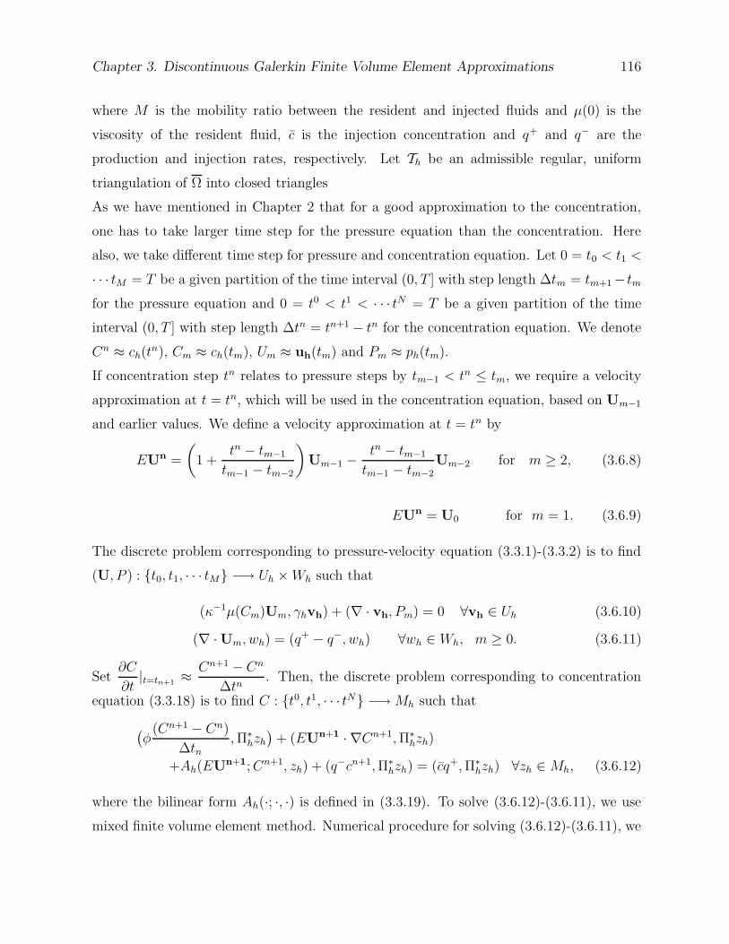
Chapter 3. Discontinuous Galerkin Finite Volume Element Approximations 116
where M is the mobility ratio between the resident and injected fluids and µ(0) is the
viscosity of the resident fluid, c is the injection concentration and q+ and q− are the
production and injection rates, respectively. Let Th be an admissible regular, uniform
triangulation of Ω into closed triangles
As we have mentioned in Chapter 2 that for a good approximation to the concentration,
one has to take larger time step for the pressure equation than the concentration. Here
also, we take different time step for pressure and concentration equation. Let 0 = t0 < t1 <
· · · tM = T be a given partition of the time interval (0, T ] with step length ∆tm = tm+1− tmfor the pressure equation and 0 = t0 < t1 < · · · tN = T be a given partition of the time
interval (0, T ] with step length ∆tn = tn+1 − tn for the concentration equation. We denote
Cn ≈ ch(tn), Cm ≈ ch(tm), Um ≈ uh(tm) and Pm ≈ ph(tm).
If concentration step tn relates to pressure steps by tm−1 < tn ≤ tm, we require a velocity
approximation at t = tn, which will be used in the concentration equation, based on Um−1
and earlier values. We define a velocity approximation at t = tn by
EUn =
(
1 +tn − tm−1
tm−1 − tm−2
)
Um−1 −tn − tm−1
tm−1 − tm−2Um−2 for m ≥ 2, (3.6.8)
EUn = U0 for m = 1. (3.6.9)
The discrete problem corresponding to pressure-velocity equation (3.3.1)-(3.3.2) is to find
(U, P ) : t0, t1, · · · tM −→ Uh ×Wh such that
(κ−1µ(Cm)Um, γhvh) + (∇ · vh, Pm) = 0 ∀vh ∈ Uh (3.6.10)
(∇ · Um, wh) = (q+ − q−, wh) ∀wh ∈ Wh, m ≥ 0. (3.6.11)
Set∂C
∂t|t=tn+1
≈ Cn+1 − Cn
∆tn. Then, the discrete problem corresponding to concentration
equation (3.3.18) is to find C : t0, t1, · · · tN −→Mh such that
(
φ(Cn+1 − Cn)
∆tn,Π∗
hzh)
+ (EUn+1 · ∇Cn+1,Π∗hzh)
+Ah(EUn+1;Cn+1, zh) + (q−cn+1,Π∗hzh) = (cq+,Π∗
hzh) ∀zh ∈ Mh, (3.6.12)
where the bilinear form Ah(·; ·, ·) is defined in (3.3.19). To solve (3.6.12)-(3.6.11), we use
mixed finite volume element method. Numerical procedure for solving (3.6.12)-(3.6.11), we
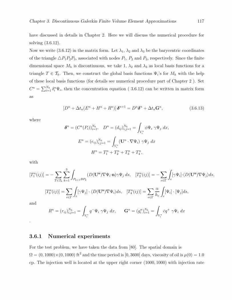
Chapter 3. Discontinuous Galerkin Finite Volume Element Approximations 117
have discussed in details in Chapter 2. Here we will discuss the numerical procedure for
solving (3.6.12).
Now we write (3.6.12) in the matrix form. Let λ1, λ2 and λ3 be the barycentric coordinates
of the triangle 4P1P2P3, associated with nodes P1, P2 and P3, respectively. Since the finite
dimensional space Mh is discontinuous, we take 1, λ2 and λ3 as local basis functions for a
triangle T ∈ Th. Then, we construct the global basis functions Ψi’s for Mh with the help
of these local basis functions (for details see numerical procedure part of Chapter 2 ). Set
Cn =∑Nh
i=1 δni Ψi, then the concentration equation ( 3.6.12) can be written in matrix form
as
[Dn + ∆tn(En +Hn +Rn)] δn+1 = Dnδn + ∆tnG
n, (3.6.13)
where
δn = (Cn(Pi))Nh
i=1, Dn = (dij)Nh
i,j=1 =
∫
V ∗
i
φΨi γΨj dx,
En = (eij)Nh
i,j=1 =
∫
V ∗
i
(Un · ∇Ψi) γΨj dx
Hn = T n1 + T n2 + T n3 + T n4 ,
with
[T n1 (ij)] = −∑
T∈Th
3∑
k=1
∫
Pk+1BPk
(D(Un)∇Ψi·n)γΨj ds, [T n2 (ij)] = −∑
e∈Γ
∫
e
[γΨi]·〈D(Un)∇Ψj〉ds,
[T n3 (ij)] =∑
e∈Γ
∫
e
[γΨj] · 〈D(Un)∇Ψi〉ds, [T n4 (ij)] =∑
e∈Γ
α
he
∫
e
[Ψi] · [Ψj]ds,
and
Rn = (rij)Nh
i,j=1 =
∫
V ∗
i
q−Ψi γΨj dx, Gn = (gni )Nh
i=1 =
∫
V ∗
i
cq+ γΨi dx
.
3.6.1 Numerical experiments
For the test problem, we have taken the data from [80]. The spatial domain is
Ω = (0, 1000)×(0, 1000) ft2 and the time period is [0, 3600] days, viscosity of oil is µ(0) = 1.0
cp. The injection well is located at the upper right corner (1000, 1000) with injection rate
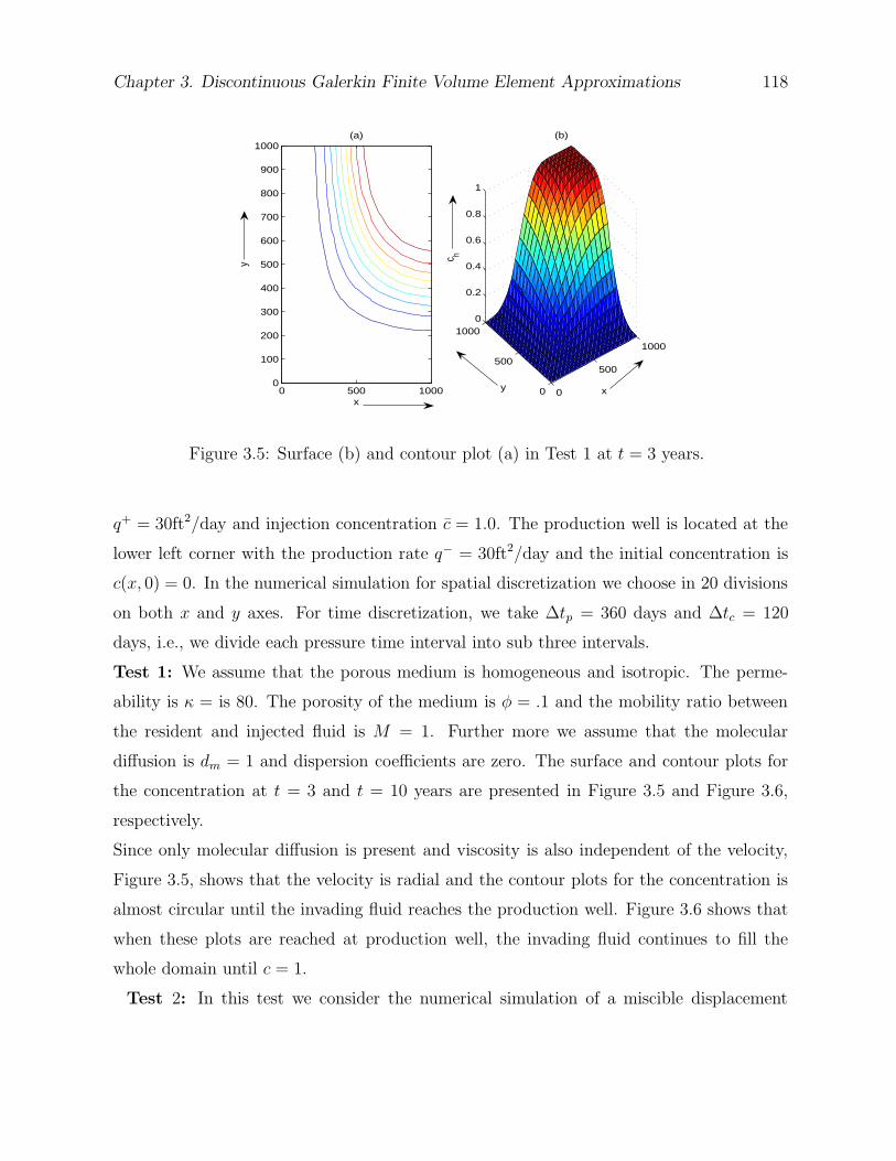
Chapter 3. Discontinuous Galerkin Finite Volume Element Approximations 118
0
500
1000
0
500
10000
0.2
0.4
0.6
0.8
1
x
(b)
y
c h
x
y
(a)
0 500 10000
100
200
300
400
500
600
700
800
900
1000
Figure 3.5: Surface (b) and contour plot (a) in Test 1 at t = 3 years.
q+ = 30ft2/day and injection concentration c = 1.0. The production well is located at the
lower left corner with the production rate q− = 30ft2/day and the initial concentration is
c(x, 0) = 0. In the numerical simulation for spatial discretization we choose in 20 divisions
on both x and y axes. For time discretization, we take ∆tp = 360 days and ∆tc = 120
days, i.e., we divide each pressure time interval into sub three intervals.
Test 1: We assume that the porous medium is homogeneous and isotropic. The perme-
ability is κ = is 80. The porosity of the medium is φ = .1 and the mobility ratio between
the resident and injected fluid is M = 1. Further more we assume that the molecular
diffusion is dm = 1 and dispersion coefficients are zero. The surface and contour plots for
the concentration at t = 3 and t = 10 years are presented in Figure 3.5 and Figure 3.6,
respectively.
Since only molecular diffusion is present and viscosity is also independent of the velocity,
Figure 3.5, shows that the velocity is radial and the contour plots for the concentration is
almost circular until the invading fluid reaches the production well. Figure 3.6 shows that
when these plots are reached at production well, the invading fluid continues to fill the
whole domain until c = 1.
Test 2: In this test we consider the numerical simulation of a miscible displacement
Chapter 3. Discontinuous Galerkin Finite Volume Element Approximations 119
0
500
1000
0
500
10000.4
0.5
0.6
0.7
0.8
0.9
1
x
(b)
y
c h
x
y
(a)
0 500 10000
100
200
300
400
500
600
700
800
900
1000
Figure 3.6: Surface (b) and contour plot (a) in Test 1 at t = 10 years.
problem with discontinuous permeability. Here, the data is same as given in Test 1 ex-
cept the permeability of the medium κ(x). We take κ = 80 on the sub domain ΩL :=
(0, 1000) × (0, 500) and κ = 20 on the sub domain ΩU := (0, 1000) × (500, 1000). The
contour and surface plot at t = 3 and t = 10 years are given in Figure 3.7 and Figure 3.8
respectively.
In Test 2, the lower half domain has a larger permeability than the upper half. Figure 3.7
and Figure 3.8 shows that when the injecting fluid reaches the lower half domain, it starts
moving much faster in the horizontal direction on this domain compared to the low perme-
ability domain that is upper half domain. We observe that one should put the production
well in a low permeability zone to increase the area swept by the injected fluid.
Order of convergence. We compute the order of convergence in the L2- norm. Figure
3.9 shows that the computed order of convergence in L2- norm is approximately 2, which
matches our theoretical findings.
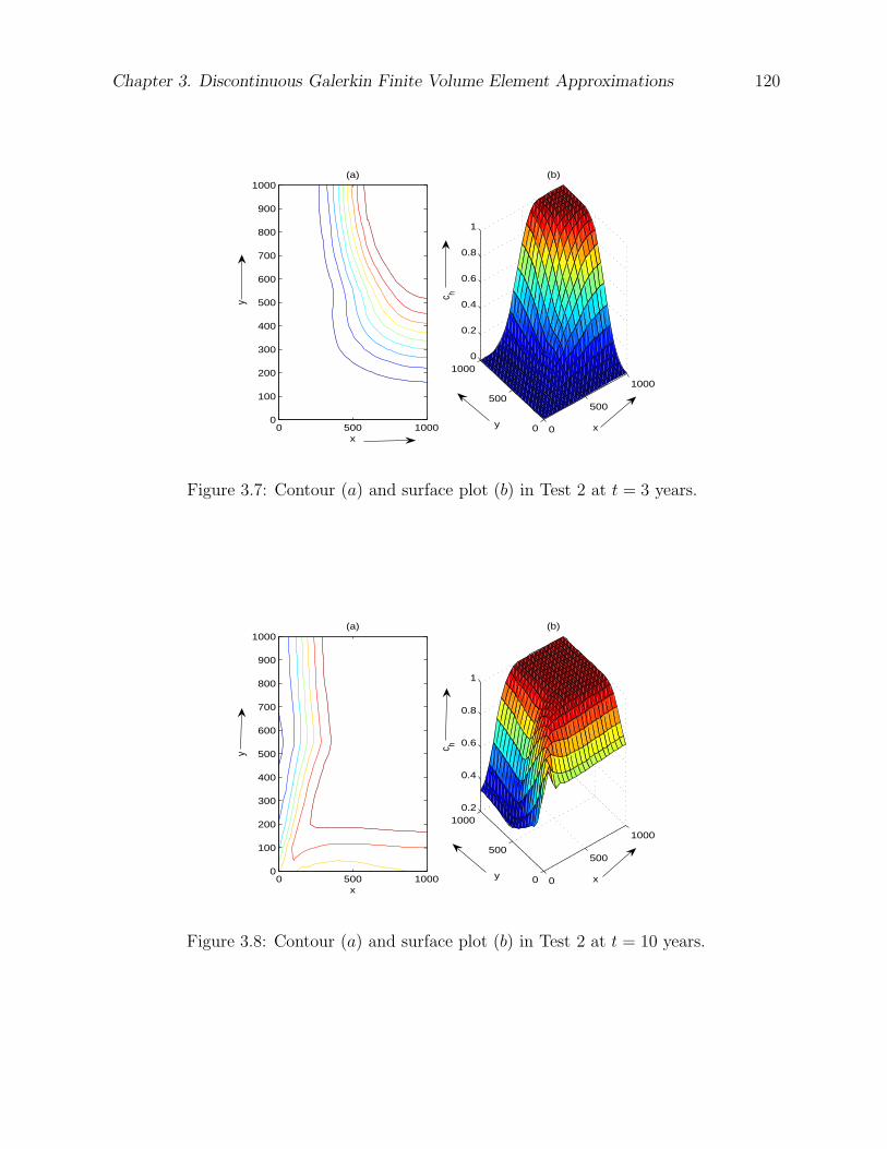
Chapter 3. Discontinuous Galerkin Finite Volume Element Approximations 120
0
500
1000
0
500
10000
0.2
0.4
0.6
0.8
1
x
(b)
y
c h
x
y
(a)
0 500 10000
100
200
300
400
500
600
700
800
900
1000
Figure 3.7: Contour (a) and surface plot (b) in Test 2 at t = 3 years.
0
500
1000
0
500
10000.2
0.4
0.6
0.8
1
x
(b)
y
c h
x
y
(a)
0 500 10000
100
200
300
400
500
600
700
800
900
1000
Figure 3.8: Contour (a) and surface plot (b) in Test 2 at t = 10 years.
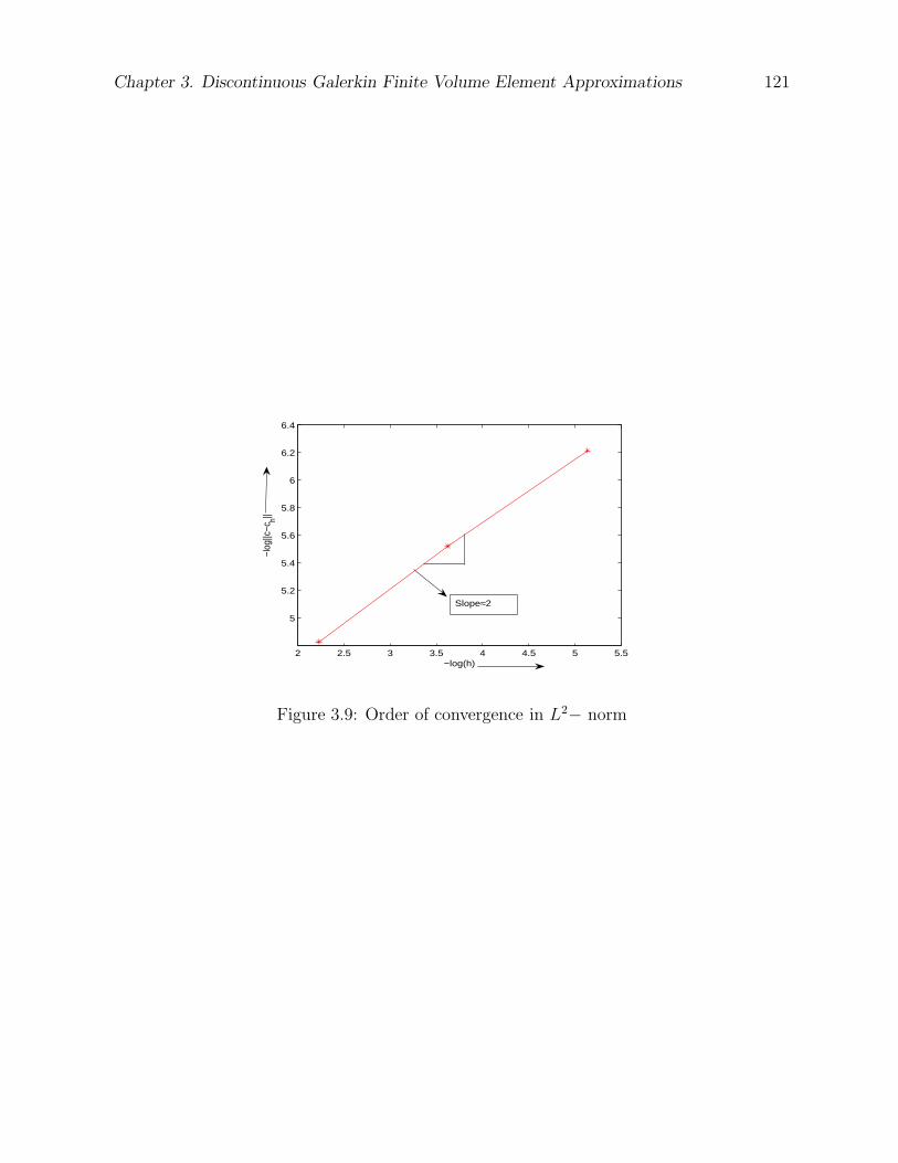
Chapter 3. Discontinuous Galerkin Finite Volume Element Approximations 121
2 2.5 3 3.5 4 4.5 5 5.5
5
5.2
5.4
5.6
5.8
6
6.2
6.4
−log(h)
−log
||c−c
h||
Slope≈2
Figure 3.9: Order of convergence in L2− norm
Chapter 4
The Modified Method of
Characteristics Combined with
FVEM
4.1 Introduction
The following system of coupled nonlinear partial differential equations describe the miscible
displacement of one incompressible fluid by another. Find the pressure p, velocity u and
the concentration c such that
u = −κ(x)µ(c)
∇p ∀(x, t) ∈ Ω × J, (4.1.1)
∇ · u = q ∀(x, t) ∈ Ω × J, (4.1.2)
φ(x)∂c
∂t+ u · ∇c−∇ · (D(u)∇c) = (c− c)q ∀(x, t) ∈ Ω × J, (4.1.3)
with boundary conditions
u · n = 0 ∀(x, t) ∈ ∂Ω × J, (4.1.4)
D(u)∇c · n = 0 ∀(x, t) ∈ ∂Ω × J, (4.1.5)
and initial condition
c(x, 0) = c0(x) ∀x ∈ Ω, (4.1.6)
122
Chapter 4. The Modified Method of Characteristics 123
where c is the concentration of the injective fluid. We assume that the domain Ω is a
rectangle and all functions in (4.1.1)-(4.1.3) are spatially Ω-periodic. This assumption on
Ω is physically reasonable, because the boundary condition (4.1.5) can be considered as a
reflection boundary and in the reservoir simulation the boundary effect are of less interest
compared to the inner flow.
As mentioned in Chapter 1, the concentration equation (4.1.3) is convection dominated
diffusion type. The standard numerical schemes fail to provide a physically relevant solu-
tion because most of these methods suffer from grid orientation effects. The other way to
minimize the grid orientation effect is to use modified methods of characteristics (MMOC).
Douglas and Russell [41] introduced and analyzed MMOC for the approximation of convec-
tion dominated diffusion equations. The authors in [34, 44, 72] studied MMOC combined
with Galerkin finite element methods for incompressible miscible displacement problems.
In this chapter, we apply MMOC combined with FVEM for the approximation of concen-
tration equation (4.1.3) and mixed FVEM for pressure-velocity equations (4.1.1)-(4.1.2).
The basic idea behind the modified method of characteristics for approximating the con-
centration equation (4.1.3) is to set the hyperbolic part, i.e., φ∂c
∂t+ u · ∇c, as a directional
derivative.
Set
ψ(x, t) = (|u(x, t)|2 + φ(x)2)1
2 = (u1(x, t)2 + u2(x, t)
2 + φ(x)2)1
2 .
The characteristic direction with respect to the operator φ∂
∂t+ u · ∇ is the unit vector
s(x, t) =(u1(x, t), u2(x, t), φ(x))
ψ(x, t).
The directional derivative of the concentration c(x, t) in the direction of s is given by
∂c
∂s=∂c
∂t
φ(x)
ψ(x, t)+
u.∇cψ(x, t)
This implies that
ψ(x, t)∂c
∂s= φ(x)
∂c
∂t+ u.∇c,
where ∇c =( ∂c
∂x,∂c
∂y
)
.
Hence, (4.1.3) can be rewritten as
ψ(x, t)∂c
∂s−∇ · (D(u)∇c) = (c− c)q ∀(x, t) ∈ Ω × J. (4.1.7)
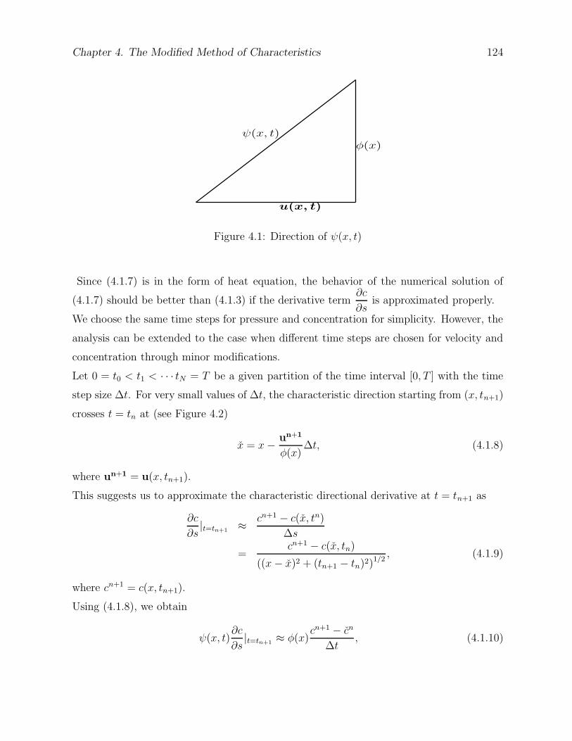
Chapter 4. The Modified Method of Characteristics 124
u(x, t)
ψ(x, t)φ(x)
Figure 4.1: Direction of ψ(x, t)
Since (4.1.7) is in the form of heat equation, the behavior of the numerical solution of
(4.1.7) should be better than (4.1.3) if the derivative term∂c
∂sis approximated properly.
We choose the same time steps for pressure and concentration for simplicity. However, the
analysis can be extended to the case when different time steps are chosen for velocity and
concentration through minor modifications.
Let 0 = t0 < t1 < · · · tN = T be a given partition of the time interval [0, T ] with the time
step size ∆t. For very small values of ∆t, the characteristic direction starting from (x, tn+1)
crosses t = tn at (see Figure 4.2)
x = x− un+1
φ(x)∆t, (4.1.8)
where un+1 = u(x, tn+1).
This suggests us to approximate the characteristic directional derivative at t = tn+1 as
∂c
∂s|t=tn+1
≈ cn+1 − c(x, tn)
∆s
=cn+1 − c(x, tn)
((x− x)2 + (tn+1 − tn)2)1/2, (4.1.9)
where cn+1 = c(x, tn+1).
Using (4.1.8), we obtain
ψ(x, t)∂c
∂s|t=tn+1
≈ φ(x)cn+1 − cn
∆t, (4.1.10)
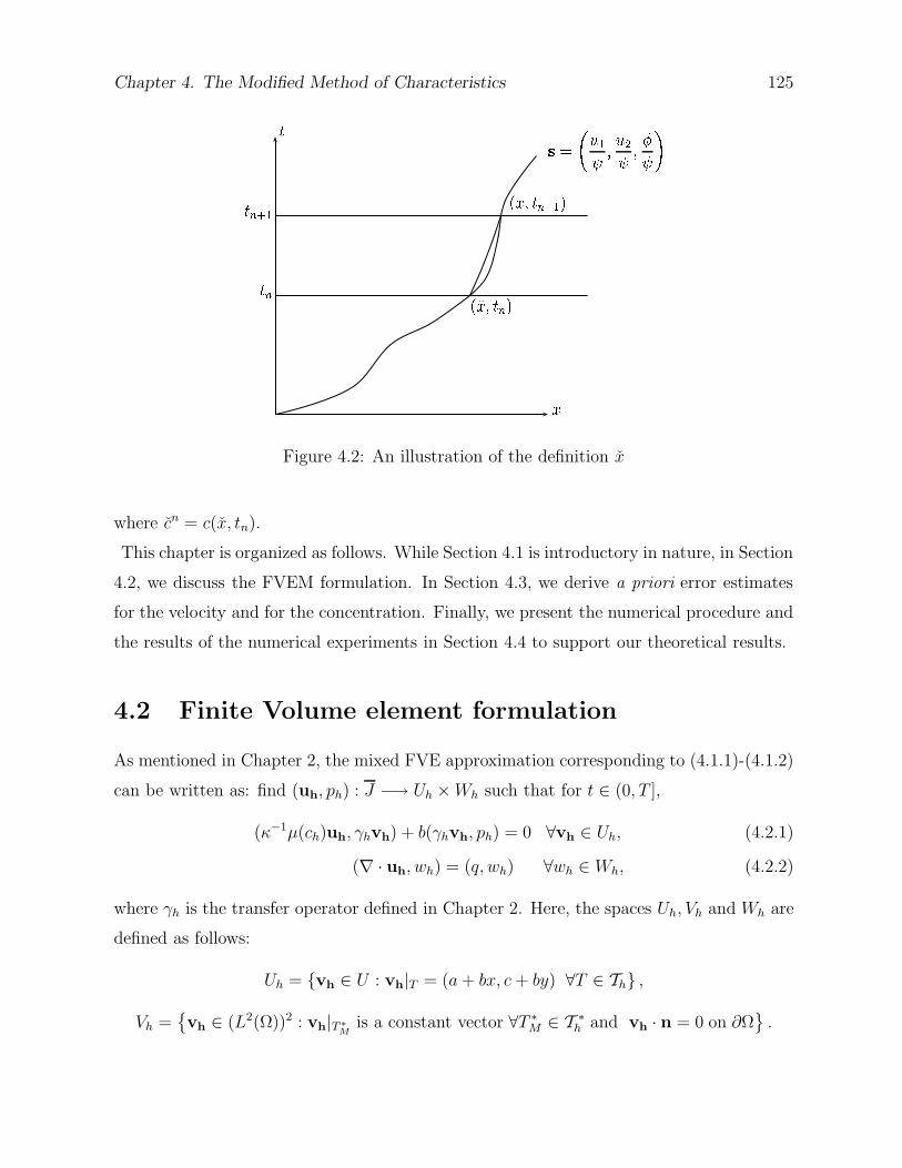
Chapter 4. The Modified Method of Characteristics 125
Figure 4.2: An illustration of the definition x
where cn = c(x, tn).
This chapter is organized as follows. While Section 4.1 is introductory in nature, in Section
4.2, we discuss the FVEM formulation. In Section 4.3, we derive a priori error estimates
for the velocity and for the concentration. Finally, we present the numerical procedure and
the results of the numerical experiments in Section 4.4 to support our theoretical results.
4.2 Finite Volume element formulation
As mentioned in Chapter 2, the mixed FVE approximation corresponding to (4.1.1)-(4.1.2)
can be written as: find (uh, ph) : J −→ Uh ×Wh such that for t ∈ (0, T ],
(κ−1µ(ch)uh, γhvh) + b(γhvh, ph) = 0 ∀vh ∈ Uh, (4.2.1)
(∇ · uh, wh) = (q, wh) ∀wh ∈ Wh, (4.2.2)
where γh is the transfer operator defined in Chapter 2. Here, the spaces Uh, Vh and Wh are
defined as follows:
Uh = vh ∈ U : vh|T = (a+ bx, c + by) ∀T ∈ Th ,
Vh =
vh ∈ (L2(Ω))2 : vh|T ∗
Mis a constant vector ∀T ∗
M ∈ T ∗h and vh · n = 0 on ∂Ω
.
Chapter 4. The Modified Method of Characteristics 126
and
Wh = wh ∈ W : wh|T is a constant ∀T ∈ Th .
Let us define the discrete norm for vh = (v1h, v
2h) ∈ Uh as
‖vh‖21,h = ‖vh‖2
(L2(Ω))2 + |vh|21,h, (4.2.3)
where |vh|21,h =∑
T∈Th
‖∇v1h‖2
0,T + ‖∇v2h‖2
0,T . For vh ∈ Uh, it is straight forward to check that
‖vh‖1,h ≤ C‖vh‖H(div;Ω), (4.2.4)
where C is a constant independent of h. For vh ∈ Uh the following inequality
‖vh‖(L∞(Ω))2 ≤ C
(
log1
h
)1/2
‖vh‖1,h, (4.2.5)
holds true when Ω is in R2 and the triangulation Th is quasi-uniform and can be proved
using the same arguments as in the proof of Lemma 4 in [78, pp. 67].
For applying the standard finite volume element method to approximate the concentration,
we define the trial space Mh on Th and the test space Lh on V∗h as follows:
Mh =
zh ∈ C0(Ω) : zh|T ∈ P1(T ) ∀T ∈ Th
Lh =
wh ∈ L2(Ω) : wh|V ∗
Pis a constant ∀V ∗
P ∈ V∗h
.
We now recall the transfer operator Π∗h : Mh −→ Lh which is defined as
Π∗hzh(x) =
Nh∑
j=1
zh(Pj)χj(x) ∀x ∈ Ω, (4.2.6)
where χj’s are the characteristic functions corresponding to the control volume V ∗Pj
, i.e.,
χj(x) =
1, if x ∈ V ∗Pj
0, elsewhere.
For any given v ∈ U, χ ∈ H1(Ω) and ψh ∈ Lh, we define the bilinear form ah(v; ·, ·) as
ah(v;χ, ψh) = −Nh∑
j=1
∫
∂V ∗
Pj
(
D(v)∇χ · nPj
)
Π∗hψhds,
Chapter 4. The Modified Method of Characteristics 127
where nPjis the unit outward normal to the boundary of V ∗
Pj.
Then, the FVE approximation corresponding to the concentration equation (4.1.7) is to
find a solution ch : J −→Mh such that for t ∈ (0, T ],
(
ψ∂ch∂s
,Π∗hzh)
+ ah(uh; ch, zh) + (chq,Π∗hzh) = (cq,Π∗
hzh) ∀zh ∈Mh (4.2.7)
ch(0) = c0,h,
where c0,h is an approximation to c0 to be defined later.
To approximate the concentration at any time say tn+1, we use the approximation to the
velocity at the previous time step. The fully discrete scheme corresponding to (4.2.1),
(4.2.2) and (4.2.7) is defined as: For n = 0, 1 · · ·N , find (cnh, pnh,u
nh) ∈ Mh ×Wh × Uh such
that
c0h = Rhc(0), (4.2.8)
(κ−1µ(cnh)unh, γhvh) + b(γhvh, p
nh) = 0 ∀vh ∈ Uh, (4.2.9)
(∇ · unh, wh) = (qn, wh) ∀wh ∈ Wh, (4.2.10)
(
φcn+1h − cnh
∆t,Π∗
hχh
)
+ ah(unh; cn+1
h , χh) + (qn+1cn+1h ,Π∗
hχh)
= (qn+1cn+1,Π∗hχh) ∀χh ∈Mh, (4.2.11)
where cnh = ch(x, tn) = ch(x−un
h
φ∆t, tn) and Rhc is a projection of c onto Mh which will be
defined in (4.3.3).
Note that in (4.1.9), we use the following notation for the exact velocity
cn = c(x, tn) = c(x− un+1
φ∆t, tn).
4.3 A priori error estimates
In this section, we derive a priori error estimates for the concentration and the velocity. We
have derived the following estimates for u and p in terms of the concentration in Chapter
2 (see Theorem 2.4.1).
Chapter 4. The Modified Method of Characteristics 128
Theorem 4.3.1 Assume that the triangulation Th is quasi-uniform. Let (u, p) and (uh, ph),
respectively, be the solutions of (4.1.1)-(4.1.2) and (4.2.1)-(4.2.2). Then, there exists a pos-
itive constant C, independent of h, but dependent on the bounds of κ−1 and µ such that
‖u − uh‖(L2(Ω))2 + ‖p− ph‖ ≤ C[
‖c− ch‖ + h(‖u‖(H1(Ω))2 + ‖p‖1)]
, (4.3.1)
‖∇ · (u − uh)‖ ≤ Ch‖∇ · u‖1, (4.3.2)
provided u(t) ∈ (H1(Ω))2, ∇ · u(t) ∈ H1(Ω) and p(t) ∈ H1(Ω), for t ∈ (0, T ] a.e.
Let Rh : H1(Ω) −→Mh be the projection of c defined by
A(u; c−Rhc, χ) = 0 ∀χ ∈Mh, (4.3.3)
where
A(u;ψ, χ) = ah(u;ψ, χ) + (qψ, χ) + (λψ, χ) ∀χ ∈Mh. (4.3.4)
The function λ will be chosen such that the coercivity of A(u; ·, ·) is assured.
The following lemma, which gives a bound for the error between the bilinear forms ah(u; ·, ·)and a(u; ·, ·), can be proved using similar arguments as used in Lemma 2.4.2 of Chapter 2.
Lemma 4.3.1 There exists a positive constant C such that
|εa(u; c−Rhc, χh)| ≤ Ch2
(
|(c− c)q|1 + |ψ∂c∂s
|1 + ‖c‖2
)
|χh|1 ∀χh ∈Mh. (4.3.5)
We also state the following lemma, which gives us H1- norm error estimates for the operator
Rh and can be easily proved using the similar arguments as in proof of Lemma 2.4.1.
Lemma 4.3.2 There exists a positive constant C independent of h such that
‖c−Rhc‖1 ≤ Ch‖c‖2, (4.3.6)
provided c(t) ∈ H2(Ω), for t ∈ (0, T ] a.e.
We also recall the following lemma from Chapter 2.
Chapter 4. The Modified Method of Characteristics 129
Lemma 4.3.3 There exists a positive constant C such that ∀θ ∈Mh,
|ah(u;Rhc, θ) − ah(uh;Rhc, θ)| ≤ C(
‖u − uh‖(L2(Ω))2 + h‖∇ · (u − uh)‖)
|θ|1. (4.3.7)
In the next lemma, we state the error estimate for Rh in L2- norm, the proof of which can
be obtained by a modification of Lemma 2.4.3 in Chapter 2.
Lemma 4.3.4 There exists a positive constant C independent of h such that
‖c−Rhc‖ ≤ Ch2
(
|(c− c)q|1 + |ψ∂c∂s
|1 + ‖c‖2
)
, (4.3.8)
provided c ∈ H2(Ω) and ψ∂c
∂s∈ H1(Ω) for t ∈ (0, T ] a.e.
Before proving the main theorem, we prove the following two lemmas for our future use.
Lemma 4.3.5 For f ∈ H1(Ω) , there exists a positive constant C independent of h and ∆t
such that
∥
∥f − f∥
∥ ≤ C∆t‖∇fn‖, (4.3.9)
where f = f(x) = f(
x− un+1(x)
φ(x)∆t)
.
Proof. Note that
∥
∥f − f∥
∥
2=
∫
Ω
(
f − f)2dx
=
∫
Ω
(∫ x
x
∇f · dθ)2
dx (4.3.10)
where θ = (1− z)x+ zx, with z ∈ [0, 1] parametrizes the line segment joining x to x. Then,
∥
∥f − f∥
∥
2 ≤∫
Ω
[∫ 1
0
(x− x)2dz
]1/2[
∫ 1
0
(
∂f
∂z((1 − z)x+ zx)
)2
dz|x]1/2
dx, (4.3.11)
where z is the unit vector in the direction of x− x and∂fn
∂zis the directional derivative of
f in the direction of z.
Since |x− x| ≤ ∆t
∣
∣
∣
∣
un+1(x)
φ(x)
∣
∣
∣
∣
, we find that
∥
∥f − f∥
∥
2 ≤ (∆t)2
∥
∥
∥
∥
un+1(x)
φ(x)
∥
∥
∥
∥
2
∞
∫
Ω
∫ 1
0
(
∂f
∂z((1 − z)x + zx)
)2
dzdx (4.3.12)
Chapter 4. The Modified Method of Characteristics 130
Define the transformation
y = Gz(x) = (1 − z)x + zx = x− un+1(x)
φ(x)∆t(1 − z). (4.3.13)
The Jacobian of the map Gz, say DGz with un+1 = (un+11 , un+1
2 ) is given by
DGz =
1 − ∂∂x1
(
un+1
1(x)
φ(x)∆t(1 − z)
)
− ∂∂x2
(
un+1
1(x)
φ(x)∆t(1 − z)
)
− ∂∂x1
(
un+1
2(x)
φ(x)∆t(1 − z)
)
1 − ∂∂x2
(
un+1
2(x)
φ(x)∆t(1 − z)
)
.
Since un+1 and its first order partial derivatives are bounded, the determinant of DGz is
of the form 1 +O(∆t).
A change in the order of integration and variables in (4.3.12) yields
∥
∥fn − f∥
∥
2 ≤ C(∆t)2
∫ 1
0
∑
T∈Th
∫
Gz(T )
∣
∣
∣
∣
∂f
∂z(y)
∣
∣
∣
∣
2
dxdz. (4.3.14)
For small ∆t it can been seen that Gz is one-one mapping on each T . Moreover, for small h
and ∆t, Gz maps T into itself and its its immediate-neighbor element. Hence, Gz is globally
at most finitely one-one and maps Ω into itself and its immediate-neighbor periodic copies.
Thus the sum in (4.3.14) is bounded by finite many multiples of an Ω- integral. This implies
that
∥
∥f − f∥
∥ ≤ C∆t‖∇f‖. (4.3.15)
Lemma 4.3.6 [41, pp. 875] If η ∈ L2(Ω) and η(x) = η(x) with x = x − r(x)∆t, for a
nonzero function r(x) such that r and ∇ · r are bounded, then
‖η − η‖−1 ≤ C‖η‖∆t, (4.3.16)
where C is a positive constant independent of h and ∆t.
Proof. Let z = G(x) = x − r(x)∆t. For sufficiently small ∆t, the determinant of DG is
nonzero. It can be easily seen that the determinant of DG and DG−1 are both of the form
1 +O(∆t).
Using the definition of ‖ · ‖−1 norm, we have
‖η − η‖−1 = supf∈H1(Ω)/0
(
1
‖f‖1
∫
Ω
[η(x) − η(x− r(x)∆t)] f(x)dx
)
. (4.3.17)
Chapter 4. The Modified Method of Characteristics 131
Using a change of variable in the second term of the right hand side of (4.3.17), we obtain
‖η − η‖−1 = supf∈H1(Ω)/0
(
1
‖f‖1
[∫
Ω
η(x)f(x)dx−∫
Ω
η(x)f(G−1(x)) detDG−1(x)dx
])
≤ supf∈H1(Ω)/0
1
‖f‖1
[∫
Ω
η(x)f(x)(
1 − detDG−1(x))
dx
]
+ supf∈H1(Ω)/0
1
‖f‖1
[∫
Ω
η(x)(
f(x) − f(G−1(x)))
detDG−1(x)dx
]
= W1 +W2, say. (4.3.18)
Since |1 − detDG−1(x)| ≤ C∆t. Hence,
|W1| ≤ C∆t supf∈H1(Ω)/0
1
‖f‖1‖f‖‖η‖ ≤ C∆t‖η‖. (4.3.19)
To bound W2, we proceed as follows. Using the Cauchy-Schwarz inequality and the fact
that | detDG−1| ≤ C, we have
|W2| ≤ C supf∈H1(Ω)/0
1
‖f‖1
‖η(x)‖ ‖f(x) − f(G−1(x))‖. (4.3.20)
Note that
‖f(x) − f(G−1(x))‖2 =
∫
Ω
[
f(x) − f(G−1(x))]2
dx. (4.3.21)
Proceeding as in the proof of Lemma 4.3.5, we obtain
‖f(x) − f(G−1(x)‖ ≤ C(∆t)‖f‖1. (4.3.22)
Substituting (4.3.22) in (4.3.20), we obtain
|W2| ≤ C∆t‖η‖. (4.3.23)
Substitute (4.3.19) and (4.3.23) in (4.3.18) to complete the rest of the proof.
Now, we prove our main theorem.
Theorem 4.3.2 Let cn and cnh be the solutions of (4.1.3) and (4.2.11) at t = tn respectively,
and let ch(0) = c0,h = Rhc(0). Further assume that ∆t = O(h). Then, for sufficiently small
Chapter 4. The Modified Method of Characteristics 132
h, there exists a positive constant C(T ) independent of h but dependent on the bounds of
κ−1 and µ such that
max0≤n≤N
‖cn − cnh‖2(L2(Ω))2 ≤ C
[
h4(
‖(c− c)q‖2L∞(0,T ;H1) + ‖ψ∂c
∂s‖2L∞(0,T ;H1) + ‖c‖2
L∞(0,T ;H2)
+‖∇.u‖2L∞(0,T ;H1) + ‖ct‖2
L∞(0,T ;H2) + ‖ψ ∂2c
∂t∂s‖2L∞(0,T ;H1)
)
+(∆t)2(
‖ut‖2L2(0,T ;(L2(Ω))2) + ‖(∇ · u)t‖2
L2(0,T ;L2) + ‖ ∂2c
∂τ 2‖2L2(0,T,L2)
)
+h2(
‖u‖2L∞(0,T ;(H1(Ω))2) + ‖p‖2
L∞(0,T ;H1)
)]
. (4.3.24)
Proof. Write cn − cnh = (cn −Rhcn) − (cnh −Rhc
n) = ρn − θn. Since the estimates of ρn are
known, it is enough to estimate θn.
Multiplying (4.1.3) by Π∗hχh and subtracting the resulting equation from (4.2.11) at t =
tn+1, we obtain
(
φcn+1h − cnh
∆t,Π∗
hχh
)
+ ah(unh; cn+1
h , χh) − ah(un+1; cn+1, χh) + (qn+1cn+1
h ,Π∗hχh)
− (qn+1cn+1,Π∗hχ) =
(
un+1 · ∇cn+1 + φ∂cn+1
∂t,Π∗
hχh
)
∀χh ∈Mh. (4.3.25)
Choose χh = θn+1 in (4.3.25) and use the definition of Rh to obtain
(
φθn+1 − θn
∆t,Π∗
hθn+1
)
+ ah(unh; θn+1, θn+1) = (θn+1qn+1,Π∗
hθn+1)
+(ρn+1, θn+1) + (ρn+1qn+1, θn+1 − Π∗hθ
n+1)
+[
ah(un+1;Rhc
n+1, θn+1) − ah(un+1h ;Rhc
n+1, θn+1)]
+(
un+1 · ∇cn+1 + φ∂cn+1
∂t− φ
(cn+1 − cn)
∆t,Π∗
hθn+1)
+
(
φ(ρn+1 − ρn)
∆t,Π∗
hθn+1
)
−(
φ(θn − θn)
∆t,Π∗
hθn+1
)
+
(
φ(Rhc
n − Rhcn)
∆t,Π∗
hθn+1
)
= T1 + T2 + T3 + T4 + T5 + T6 + T7 + T8. (4.3.26)
Chapter 4. The Modified Method of Characteristics 133
To estimate T1, T2 and T3, we use the Cauchy-Schwarz inequality, boundedness of q and
(2.3.47) to obtain
|T1| = |(θn+1qn+1,Π∗hθ
n+1)| ≤ C‖θn+1‖2, (4.3.27)
|T2| = |(ρn+1, θn+1)| ≤ C‖ρn+1‖ ‖θn+1‖, (4.3.28)
and
|T3| = |(ρn+1qn+1, θn+1 − Π∗hθ
n+1)| ≤ C‖ρn+1‖ ‖θn+1‖. (4.3.29)
To bound T4, we use Lemma 4.3.3 to obtain
|T4| = |ah(un+1;Rhcn+1, θn+1) − ah(u
n+1h ;Rhc
n+1, θn+1)|
≤ C(
‖un+1 − unh‖(L2(Ω))2 + h‖∇ · (un+1 − un+1
h )‖)
|θn+1|1≤ C
(
‖un+1 − un‖(L2(Ω))2 + ‖un − unh‖(L2(Ω))2 + h‖∇ · (un+1 − un)‖
+h‖∇ · (un − unh)‖)
|θn+1|1. (4.3.30)
From (2.5.22) and (2.5.23), we find that
‖un+1 − un‖2(L2(Ω))2 ≤ ∆t‖ut‖2
L2(tn,tn+1;(L2(Ω))2), (4.3.31)
and
‖∇ · (un+1 − un)‖2L2(Ω) ≤ ∆t‖(∇ · u)t‖2
L2(tn ,tn+1;L2). (4.3.32)
Hence,
|T4| ≤ C[
(∆t)1/2(
‖ut‖L2(tn,tn+1,(L2(Ω))2) + h‖(∇ · u)t‖L2(tn ,tn+1,L2(Ω))
)
+‖un − unh‖(L2(Ω))2 + h‖∇ · (un − uh
n)‖]
|θn+1|. (4.3.33)
Using the Cauchy- Schwarz inequality and (2.3.47), we obtain
|T5| =
∣
∣
∣
∣
(
un+1 · ∇cn+1 + φ∂cn+1
∂t− φ
(cn+1 − cn)
∆t,Π∗
hθn+1)
∣
∣
∣
∣
≤ C
∥
∥
∥
∥
un+1 · ∇cn+1 + φ∂cn+1
∂t− φ
(cn+1 − cn)
∆t
∥
∥
∥
∥
‖θn+1‖. (4.3.34)
Chapter 4. The Modified Method of Characteristics 134
To bound
∥
∥
∥
∥
un+1 · ∇cn+1 + φ∂cn+1
∂t− φ
(cn+1 − cn)
∆t
∥
∥
∥
∥
, we use the similar arguments given in
[44]. Let σ(x) = [φ(x)2 + un+1(x)2]1/2
, so that
φ∂cn+1
∂t+ un+1 · ∇cn+1 = σ
∂cn+1
∂τ. (4.3.35)
where τ approximates the characteristic unit vector s. Let τ ∈ [0, 1] parametrize the
approximate characteristic tangent from (x, tn)[τ = 0] to (x, tn+1)[τ = 1]. A use of Taylor
expansion along the characteristic gives us
σ∂cn+1
∂τ− φ
cn+1 − cn
∆t=
φ
∆t
∫ (x,tn+1)
(x,tn)
[|x(τ) − x|2 + (t(τ) − tn)2]1/2
∂2c
∂τ 2dτ. (4.3.36)
Taking the square of the L2(Ω) norm, we obtain
∥
∥
∥
∥
σ∂cn+1
∂τ− φ
cn+1 − cn
∆t
∥
∥
∥
∥
2
≤∫
Ω
[
φ
∆t
]2 [σ∆t
φ
]2∣
∣
∣
∣
∣
∫ (x,tn+1)
(x,tn)
∂2c
∂τ 2dτ
∣
∣
∣
∣
∣
2
dx.
Using the Cauchy-Schwarz inequality, we find that
∥
∥
∥
∥
σ∂cn+1
∂τ− φ
cn+1 − cn
∆t
∥
∥
∥
∥
2
≤ ∆t
∥
∥
∥
∥
σ3
φ
∥
∥
∥
∥
∞
∫
Ω
∫ (x,tn+1)
(x,tn)
∣
∣
∣
∣
∂2c
∂τ 2
∣
∣
∣
∣
2
dτdx
≤ ∆t
∥
∥
∥
∥
σ4
φ2
∥
∥
∥
∥
∞
∫
Ω
∫ tn+1
tn
∣
∣
∣
∣
∂2c
∂τ 2(τ x + (1 − τ )x, t)
∣
∣
∣
∣
2
dtdx.(4.3.37)
For a fixed τ consider the transformation
y = fτ = τ x + (1 − τ )x = x− un+1
φ∆tτ .
Since u, φ and their first order partial derivatives are bounded, the determinant of Dfτ is
1 + O(∆t) and hence Dfτ is invertible for sufficiently small ∆t. By a change of variable
argument, we have
∥
∥
∥
∥
σ∂cn+1
∂τ− φ
cn+1 − cn
∆t
∥
∥
∥
∥
2
≤ C∆t‖ ∂2c
∂τ 2‖2L2(tn,tn+1;L2). (4.3.38)
Hence, T5 bounded as follows
|T5| ≤ C(∆t)1/2‖ ∂2c
∂τ 2‖L2(tn,tn+1;L2)‖θn+1‖. (4.3.39)
Chapter 4. The Modified Method of Characteristics 135
To bound T6, we proceed as follows
|T6| =
∣
∣
∣
∣
(
φ(ρn+1 − ρn)
∆t,Π∗
hθn+1
)∣
∣
∣
∣
≤∣
∣
∣
∣
(
φ(ρn+1 − ρn)
∆t, θn+1 − Π∗
hθn+1
)∣
∣
∣
∣
+
∣
∣
∣
∣
(
φ(ρn+1 − ρn)
∆t, θn+1
)∣
∣
∣
∣
= I1 + I2. (4.3.40)
Now I1 can be written as
I1 ≤∣
∣
∣
∣
(
φ(ρn+1 − ρn)
∆t, θn+1 − Π∗
hθn+1
)∣
∣
∣
∣
+
∣
∣
∣
∣
(
φ(ρn − ρn)
∆t, θn+1 − Π∗
hθn+1
)∣
∣
∣
∣
. (4.3.41)
A use of Lemma 4.3.5 yields∥
∥
∥
∥
(ρn − ρn)
∆t
∥
∥
∥
∥
≤ C‖∇ρn‖. (4.3.42)
It is easy to show that∥
∥
∥
∥
(ρn+1 − ρn)
∆t
∥
∥
∥
∥
≤ C(∆t)−1/2‖∂ρ∂t
‖L2(tn ,tn+1,L2). (4.3.43)
Using (4.3.42), (4.3.43), (2.3.16) and the Cauchy-Schwarz inequality, we obtain
I1 ≤ C
[
‖θn+1 − Π∗hθ
n+1‖(
(∆t)−1/2‖∂ρ∂t
‖L2(tn,tn+1,L2) + ‖∇ρn‖)]
≤ Ch
[
(∆t)−1/2‖∂ρ∂t
‖L2(tn ,tn+1,L2) + ‖∇ρn‖]
‖∇θn+1‖. (4.3.44)
I2 can be bounded as follows:
I2 ≤∣
∣
∣
∣
(
φ(ρn+1 − ρn)
∆t, θn+1
)∣
∣
∣
∣
+
∣
∣
∣
∣
(
φ(ρn − ρn)
∆t, θn+1
)∣
∣
∣
∣
= J1 + J2. (4.3.45)
A use of Cauchy-Schwarz inequality yields
J1 ≤ C(∆t)−1/2‖∂ρ∂t
‖L2(tn,tn+1,L2)‖θn+1‖. (4.3.46)
Using Lemma 4.3.6, we obtain
J2 ≤ C
∥
∥
∥
∥
(ρn − ρn)
∆t
∥
∥
∥
∥
−1
‖θn+1‖1 ≤ C‖ρn‖‖θn+1‖1. (4.3.47)
This implies that
I2 ≤ C
(
(∆t)−1/2‖∂ρ∂t
‖L2(tn,tn+1,L2) + ‖ρn‖)
‖θn+1‖. (4.3.48)
Chapter 4. The Modified Method of Characteristics 136
Using (4.3.44), (4.3.48) and (4.3.40), we obtain the following bound for T6:
|T6| ≤ C
(
(∆t)−1/2‖∂ρ∂t
‖L2(tn ,tn+1,L2) + h‖∇ρn‖ + ‖ρn‖)
‖θn+1‖. (4.3.49)
Using the Cauchy-Schwarz inequality, we obtain
|T7| ≤∣
∣
∣
∣
∣
(
(θn − θn)
∆t,Π∗
hθn+1 − θn+1
)∣
∣
∣
∣
∣
+
∣
∣
∣
∣
∣
(
(θn − θn)
∆t, θn+1
)∣
∣
∣
∣
∣
≤∥
∥
∥
∥
∥
(θn − θn)
∆t
∥
∥
∥
∥
∥
‖Π∗hθ
n+1 − θn+1‖ +
∥
∥
∥
∥
∥
(θn − θn)
∆t
∥
∥
∥
∥
∥
−1
‖θn+1‖1. (4.3.50)
We use Lemma 4.3.5 and Lemma 4.3.6 to bound
∥
∥
∥
∥
∥
θn − θn
∆t
∥
∥
∥
∥
∥
and
∥
∥
∥
∥
∥
θn − θn
∆t
∥
∥
∥
∥
∥
−1
, respectively.
For this, we need that unh and its first derivative are bounded.
First let us make an induction hypothesis. Let there is a constant say K∗ ≥ 2K with
‖unh‖(L∞(Ω))2 ≤ K such that
‖unh‖(L∞(Ω))2 ≤ K∗, (4.3.51)
where uh is the projection of uh at t = tn defined by (see Chapter 2, (2.4.8)-(2.4.9))
(κ−1µ(c)uh,vh) − (∇ · vh, ph) = 0 ∀vh ∈ Uh, (4.3.52)
(∇ · uh, wh) = (q, wh) ∀wh ∈ Wh. (4.3.53)
To bound ‖∇.unh‖∞, we use inverse inequality and (4.3.51)
‖∇.unh‖∞∆t ≤ Ch−1∆t‖un
h‖∞ ≤ C. (4.3.54)
where we have used the assumption that ∆t = O(h).
Using Lemma 4.3.5, we have∥
∥
∥
∥
∥
θn − θn
∆t
∥
∥
∥
∥
∥
≤ C(K∗)‖∇θn‖. (4.3.55)
Similar arguments as in the proof of Lemma 4.3.6, gives∥
∥
∥
∥
∥
θn − θn
∆t
∥
∥
∥
∥
∥
−1
≤ C(K∗)‖θn‖. (4.3.56)
Chapter 4. The Modified Method of Characteristics 137
Now using (2.3.16), (4.3.55), inverse inequality (2.3.15) and (4.3.56), we obtain the following
bound for T7:
|T7| ≤ C(K∗)‖θn‖ ‖θn+1‖1. (4.3.57)
To bound T8, we use maximum norm estimate of ∇Rhc (see (2.4.43)).∥
∥
∥
∥
∥
Rhcn − Rhc
n
∆t
∥
∥
∥
∥
∥
≤ ‖Rhc‖1,∞‖un − unh‖ ≤ C‖un − un
h‖(L2(Ω))2 , (4.3.58)
and hence, using (2.3.47), T8 is bounded as follows
T8 ≤ C‖θn+1‖ ‖un − unh‖(L2(Ω))2 . (4.3.59)
Substitute the estimates of T1, T2 · · ·T8 in (4.3.26) and use non-singular property of φ, kick
back argument with the Young’s inequality to obtain
1
∆t
[
(θn+1,Π∗hθ
n+1) − (θn,Π∗hθ
n+1)]
≤ C(K∗)[
∆t−1‖∂ρ∂t
‖2L2(tn ,tn+1,L2) + ‖θn+1‖2
+‖θn+1‖21 + ‖θn‖2 + ‖ρn+1‖2 + ∆t
(
‖ut‖2L2(tn ,tn+1;(L2(Ω))2) + ‖∇ · u)t‖2
L2(tn,tn+1;L2
+‖ ∂2c
∂τ 2‖2L2(tn,tn+1,L2)
)
+ ‖un − unh‖2
(L2(Ω))2
+h2‖∇.(un − unh)‖2 + ‖ρn‖2 + h2‖∇ρn‖2
]
. (4.3.60)
Using (4.3.1) and (4.3.2), we obtain
‖un − unh‖(L2(Ω))2 ≤ C
[
‖cn − cnh‖ + h(
‖un‖(H1(Ω))2 + ‖pn‖21
)
]
≤ C[
‖θn‖ + ‖ρn‖ + h(
‖un‖(H1(Ω))2 + ‖pn‖21
)
]
, (4.3.61)
and
‖∇ · (un − unh)‖ ≤ Ch‖∇ · un‖1. (4.3.62)
Substitute (4.3.61) and (4.3.62) in (4.3.60) to obtain
‖|θn+1‖|2 − ‖|θn‖|2 ≤ C(K∗)[
∆t(
‖θn+1‖2 + ‖θn‖2 + ‖ρn‖2 + ‖ρn+1‖2 + h2‖∇ρn‖2)
+(∆t)2(
‖ut‖2L2(tn,tn+1;(L2(Ω))2) + ‖∇ · ut‖2
L2(tn,tn+1;L2)
+‖ ∂2c
∂τ 2‖2L2(tn,tn+1,L2)
)
+ ‖∂ρ∂t
‖2L2(tn,tn+1,L2)
+h2∆t(
h2‖∇ · un‖21 + ‖un‖2
(H1(Ω))2 + ‖pn‖21
) ]
. (4.3.63)
Chapter 4. The Modified Method of Characteristics 138
Taking summation over n = 0 · · ·m− 1, we obtain
‖|θm‖|2 − ‖|θ0‖|2 ≤ C(K∗)[
m−1∑
n=0
∆t(
‖θn+1‖2 + ‖θn‖2 + ‖ρn‖2 + ‖ρn+1‖2 + h2‖∇ρn‖2)
+(∆t)2(
‖ut‖2L2(tn,tn+1;(L2(Ω))2) + ‖∇ · ut‖2
L2(tn ,tn+1;L2) + ‖ ∂2c
∂τ 2‖2L2(tn ,tn+1,L2)
)
+‖∂ρ∂t
‖2L2(tn,tn+1;L2) + h2∆t
(
h2‖∇ · un‖21 + ‖un‖2
(H1(Ω))2 + ‖pn‖21
)]
. (4.3.64)
Now using discrete Gronwall’s ( see Lemma 1.2.8), equivalence of the norms (2.3.46) and
the estimates of ρ, we obtain
‖θm‖2 ≤ C(K∗)[
‖θ0‖2 + h4(
‖(c− c)q‖2L∞(0,T ;H1) + ‖ψ∂c
∂s‖2L∞(0,T ;H1) + ‖c‖2
L∞(0,T ;H2)
+‖∇.u‖2L∞(0,T ;H1) + ‖ct‖2
L∞(0,T ;H2) + ‖ψ ∂2c
∂t∂s‖2L∞(0,T ;H1)
)
+(∆t)2(
‖ut‖2L2(0,T ;(L2(Ω))2) + ‖∇ · ut‖2
L2(0,T ;L2) + ‖ ∂2c
∂τ 2‖2L2(0,T,L2)
)
+h2(
‖u‖2L∞(0,T ;(H1(Ω))2) + ‖p‖2
L∞(0,T ;H1)
)]
. (4.3.65)
Now it remains to show the induction hypothesis (4.3.51). Using (4.2.4) and (4.2.5), we
have
‖unh‖(L∞(Ω))2 ≤ ‖un
h − unh‖(L∞(Ω))2 + ‖un
h‖(L∞(Ω))2
≤ C(
log1
h
)1/2
‖unh − un
h‖H(div;Ω) +K.
Using ‖∇.(unh − un
h)‖ = 0, we have
‖unh − un
h‖(L∞(Ω))2 ≤ C(
log1
h
)1/2
‖unh − un
h‖(L2(Ω))2 . (4.3.66)
Now using (2.4.22) and (4.3.65), we obtain for small h
‖unh‖(L∞(Ω))2 ≤ C(K∗) log
1
h(h+ ∆t) +K ≤ 2K. (4.3.67)
Here we have used ∆t = O(h) and h log1
h−→ 0 as h → 0 and this proves our induction
hypothesis (4.3.51).
Now combine the estimates of ρ and θ and use triangle inequality to complete the rest of
the proof.
Using (4.3.1) and Theorem 4.3.2, we obtain the following error estimates for velocity as
well as pressure.
Chapter 4. The Modified Method of Characteristics 139
Theorem 4.3.3 Assume that the triangulation Th is quasi-uniform. Let (u, p) and (uh, ph)
be respectively the solutions of (4.1.1)-(4.1.2) and (4.2.1)-(4.2.2) and let ch(0) = c0,h =
Rhc(0). Further assume that ∆t = O(h). Then for sufficiently small h there exists a
positive constant C(T ) independent of h but dependent on the bounds of κ−1 and µ such
that
max0≤n≤N
‖un − unh‖2
(L2(Ω))2 ≤ C[
h4(
‖(c− c)q‖2L∞(0,T ;H1) + ‖ψ∂c
∂s‖2L∞(0,T ;H1) + ‖c‖2
L∞(0,T ;H2)
+‖∇.u‖2L∞(0,T ;H1) + ‖ct‖2
L∞(0,T ;H2) + ‖ψ ∂2c
∂t∂s‖2L∞(0,T ;H1)
)
+(∆t)2(
‖ut‖2L2(0,T ;(L2(Ω))2) + ‖∇ · ut‖2
L2(0,T ;L2) + ‖ ∂2c
∂τ 2‖2L2(0,T,L2)
)
+h2(
‖u‖2L∞(0,T ;(H1(Ω))2) + ‖p‖2
L∞(0,T ;H1)
)]
. (4.3.68)
4.4 Numerical Experiments
As mentioned in Chapter 2, we use larger time steps for the pressure equation than the
concentration equation. Let 0 = t0 < t1 < · · · tM = T be a given partition of the time
interval (0, T ] with step length ∆tm = tm+1−tm for the pressure equation and 0 = t0 < t1 <
· · · tN = T be a given partition of the time interval (0, T ] with step length ∆tn = tn+1 − tn
for the concentration equation. Let Cn, Um and Pm be the approximation values of ch, uh,
ph at t = tn and t = tm, respectively.
If concentration step tn relates to pressure steps by tm−1 < tn ≤ tm, we require a velocity
approximation at t = tn, which will be used in the concentration equation, based on Um−1
and earlier values. We define a velocity approximation [44, pp. 81] at t = tn by
EUn =
(
1 +tn − tm−1
tm−1 − tm−2
)
Um−1 −tn − tm−1
tm−1 − tm−2Um−2 for m ≥ 2, (4.4.1)
EUn = U0 for m = 1. (4.4.2)
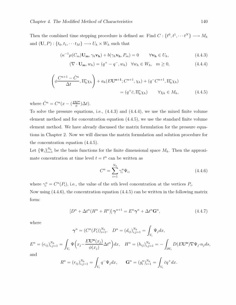
Chapter 4. The Modified Method of Characteristics 140
Then the combined time stepping procedure is defined as: Find C : t0, t1, · · · tN −→Mh
and (U, P ) : t0, t1, · · · tM −→ Uh ×Wh such that
(κ−1µ(Cm)Um, γhvh) + b(γhvh, Pm) = 0 ∀vh ∈ Uh, (4.4.3)
(∇ · Um, wh) = (q+ − q−, wh) ∀wh ∈ Wh, m ≥ 0, (4.4.4)
(
φCn+1 − Cn
∆t,Π∗
hχh
)
+ ah(EUn+1;Cn+1, χh) + (q−Cn+1,Π∗hχh)
= (q+c,Π∗hχh) ∀χh ∈Mh, (4.4.5)
where Cn = Cn(x− (EUn
φ)∆t).
To solve the pressure equations, i.e., (4.4.3) and (4.4.4), we use the mixed finite volume
element method and for concentration equation (4.4.5), we use the standard finite volume
element method. We have already discussed the matrix formulation for the pressure equa-
tions in Chapter 2. Now we will discuss the matrix formulation and solution procedure for
the concentration equation (4.4.5).
Let ΨiNh
i=1 be the basis functions for the finite dimensional space Mh. Then the approxi-
mate concentration at time level t = tn can be written as
Cn =
Nh∑
i=1
γni Ψi, (4.4.6)
where γni = Cn(Pi), i.e., the value of the nth level concentration at the vertices Pi.
Now using (4.4.6), the concentration equation (4.4.5) can be written in the following matrix
form:
[Dn + ∆tn(Hn +Rn)] γn+1 = Enγn + ∆tnGn, (4.4.7)
where
γn = (Cn(Pi))Nh
i=1, Dn = (dij)Nh
i,j=1 =
∫
Vi
Ψjdx,
En = (eij)Nh
i,j=1 =
∫
Vi
Ψ(
xj−EUn(xj)
φ(xj)∆tn
)
dx, Hn = (hij)Nh
i,j=1 = −∫
∂Vi
D(EUn)∇Ψj·njds,
and
Rn = (rij)Nh
i,j=1 =
∫
Vi
q−Ψjdx, Gn = (gni )Nh
i=1 =
∫
Vi
cq+dx.
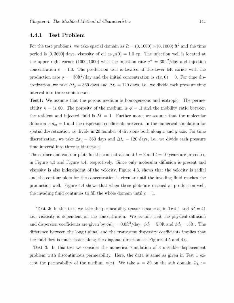
Chapter 4. The Modified Method of Characteristics 141
4.4.1 Test Problem
For the test problems, we take spatial domain as Ω = (0, 1000)× (0, 1000) ft2 and the time
period is [0, 3600] days, viscosity of oil as µ(0) = 1.0 cp. The injection well is located at
the upper right corner (1000, 1000) with the injection rate q+ = 30ft2/day and injection
concentration c = 1.0. The production well is located at the lower left corner with the
production rate q− = 30ft2/day and the initial concentration is c(x, 0) = 0. For time dis-
cretization, we take ∆tp = 360 days and ∆tc = 120 days, i.e., we divide each pressure time
interval into three subintervals.
Test1: We assume that the porous medium is homogeneous and isotropic. The perme-
ability κ = is 80. The porosity of the medium is φ = .1 and the mobility ratio between
the resident and injected fluid is M = 1. Further more, we assume that the molecular
diffusion is dm = 1 and the dispersion coefficients are zero. In the numerical simulation for
spatial discretization we divide in 20 number of divisions both along x and y axis. For time
discretization, we take ∆tp = 360 days and ∆tc = 120 days, i.e., we divide each pressure
time interval into three subintervals.
The surface and contour plots for the concentration at t = 3 and t = 10 years are presented
in Figure 4.3 and Figure 4.4, respectively. Since only molecular diffusion is present and
viscosity is also independent of the velocity, Figure 4.3, shows that the velocity is radial
and the contour plots for the concentration is circular until the invading fluid reaches the
production well. Figure 4.4 shows that when these plots are reached at production well,
the invading fluid continues to fill the whole domain until c = 1.
Test 2: In this test, we take the permeability tensor is same as in Test 1 and M = 41
i.e., viscosity is dependent on the concentration. We assume that the physical diffusion
and dispersion coefficients are given by φdm = 0.0ft2/day, φdt = 5.0ft and φdt = .5ft . The
difference between the longitudinal and the transverse dispersity coefficients implies that
the fluid flow is much faster along the diagonal direction see Figures 4.5 and 4.6.
Test 3: In this test we consider the numerical simulation of a miscible displacement
problem with discontinuous permeability. Here, the data is same as given in Test 1 ex-
cept the permeability of the medium κ(x). We take κ = 80 on the sub domain ΩL :=
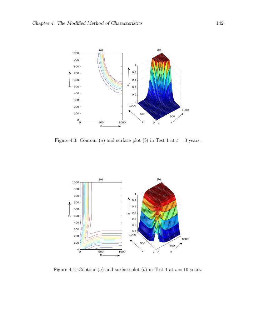
Chapter 4. The Modified Method of Characteristics 142
0
500
1000
0
500
10000
0.2
0.4
0.6
0.8
1
x
(b)
y
c hx
y
(a)
0 500 10000
100
200
300
400
500
600
700
800
900
1000
Figure 4.3: Contour (a) and surface plot (b) in Test 1 at t = 3 years.
0
500
1000
0
500
10000.4
0.5
0.6
0.7
0.8
0.9
1
x
(b)
y
c h
x
y
(a)
0 500 10000
100
200
300
400
500
600
700
800
900
1000
Figure 4.4: Contour (a) and surface plot (b) in Test 1 at t = 10 years.
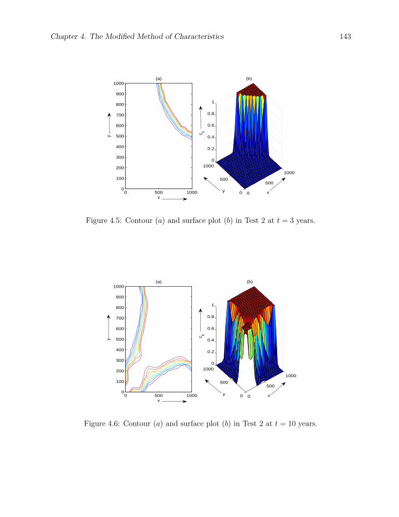
Chapter 4. The Modified Method of Characteristics 143
0
500
1000
0
500
10000
0.2
0.4
0.6
0.8
1
x
(b)
y
c h
x
y
(a)
0 500 10000
100
200
300
400
500
600
700
800
900
1000
Figure 4.5: Contour (a) and surface plot (b) in Test 2 at t = 3 years.
0
500
1000
0
500
10000
0.2
0.4
0.6
0.8
1
x
(b)
y
c h
x
y
(a)
0 500 10000
100
200
300
400
500
600
700
800
900
1000
Figure 4.6: Contour (a) and surface plot (b) in Test 2 at t = 10 years.
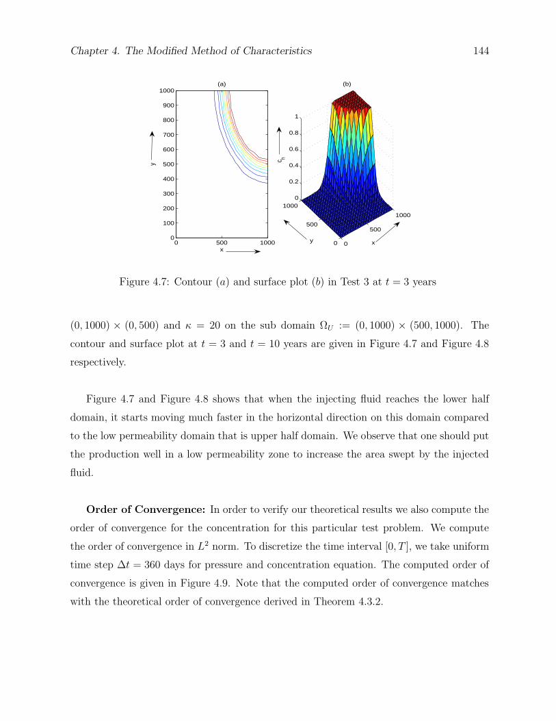
Chapter 4. The Modified Method of Characteristics 144
0
500
1000
0
500
10000
0.2
0.4
0.6
0.8
1
x
(b)
y
c h
x
y
(a)
0 500 10000
100
200
300
400
500
600
700
800
900
1000
Figure 4.7: Contour (a) and surface plot (b) in Test 3 at t = 3 years
(0, 1000) × (0, 500) and κ = 20 on the sub domain ΩU := (0, 1000) × (500, 1000). The
contour and surface plot at t = 3 and t = 10 years are given in Figure 4.7 and Figure 4.8
respectively.
Figure 4.7 and Figure 4.8 shows that when the injecting fluid reaches the lower half
domain, it starts moving much faster in the horizontal direction on this domain compared
to the low permeability domain that is upper half domain. We observe that one should put
the production well in a low permeability zone to increase the area swept by the injected
fluid.
Order of Convergence: In order to verify our theoretical results we also compute the
order of convergence for the concentration for this particular test problem. We compute
the order of convergence in L2 norm. To discretize the time interval [0, T ], we take uniform
time step ∆t = 360 days for pressure and concentration equation. The computed order of
convergence is given in Figure 4.9. Note that the computed order of convergence matches
with the theoretical order of convergence derived in Theorem 4.3.2.
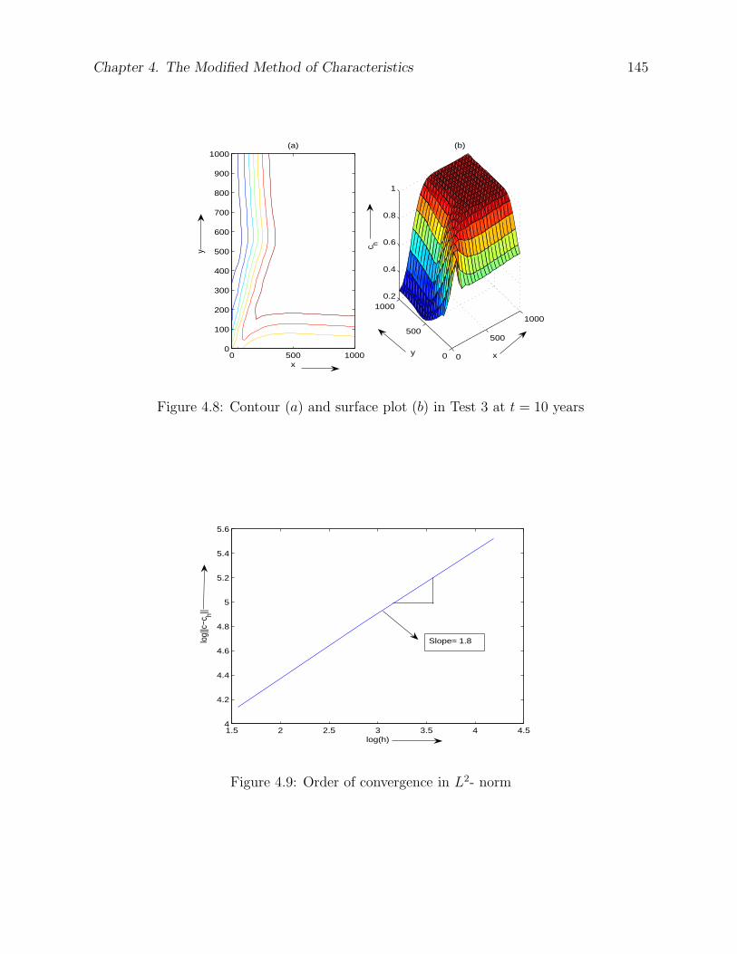
Chapter 4. The Modified Method of Characteristics 145
0
500
1000
0
500
10000.2
0.4
0.6
0.8
1
x
(b)
y
c hx
y
(a)
0 500 10000
100
200
300
400
500
600
700
800
900
1000
Figure 4.8: Contour (a) and surface plot (b) in Test 3 at t = 10 years
1.5 2 2.5 3 3.5 4 4.54
4.2
4.4
4.6
4.8
5
5.2
5.4
5.6
log(h)
log|
|c−c
h||
Slope≈ 1.8
Figure 4.9: Order of convergence in L2- norm

Chapter 5
Conclusions and Future Directions
In this thesis, an attempt has been made to study finite volume element methods for a
coupled system of nonlinear elliptic and parabolic equations arising in the incompressible
miscible displacement problems in porous media.
5.1 Summary
In Chapters 2, 3 and 4, we have applied a mixed finite volume element method for approx-
imating the pressure equation and different kinds of methods for the approximation of the
concentration equation. In Chapter 1, we have discussed briefly theoretical and computa-
tional issues related to the incompressible miscible displacement problems in porous media.
Moreover, an extensive survey for the finite volume element methods is presented.
In Chapter 2, we have applied a mixed finite volume element method for the pressure equa-
tion and a standard finite volume element method for the approximation of the concen-
tration equation. The trial space for velocity consists of the lowest order Raviart-Thomas
element while the trial space for concentration is C0- piecewise linear. We have obtained
a priori error estimates in L∞(L2) norm for the concentration as well as for the velocity,
see Theorem 2.4.2 and 2.4.3. We have also presented a couple of numerical experiments for
the verification of our theoretical findings.
In Chapter 3, we have applied a discontinuous Galerkin finite volume element method for
the approximation of the concentration equation and a mixed finite volume element method
146
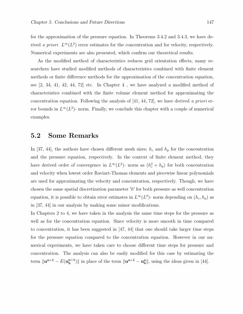
Chapter 5. Conclusions and Future Directions 147
for the approximation of the pressure equation. In Theorems 3.4.2 and 3.4.3, we have de-
rived a priori L∞(L2) error estimates for the concentration and for velocity, respectively.
Numerical experiments are also presented, which confirm our theoretical results.
As the modified method of characteristics reduces grid orientation effects, many re-
searchers have studied modified methods of characteristics combined with finite element
methods or finite difference methods for the approximation of the concentration equation,
see [2, 34, 41, 42, 44, 72] etc. In Chapter 4 , we have analyzed a modified method of
characteristics combined with the finite volume element method for approximating the
concentration equation. Following the analysis of [41, 44, 72], we have derived a priori er-
ror bounds in L∞(L2)- norm. Finally, we conclude this chapter with a couple of numerical
examples.
5.2 Some Remarks
In [37, 44], the authors have chosen different mesh sizes; hc and hp for the concentration
and the pressure equation, respectively. In the context of finite element method, they
have derived order of convergence in L∞(L2)- norm as (h2c + hp) for both concentration
and velocity when lowest order Raviart-Thomas elements and piecewise linear polynomials
are used for approximating the velocity and concentration, respectively. Though, we have
chosen the same spatial discretization parameter ′h′ for both pressure as well concentration
equation, it is possible to obtain error estimates in L∞(L2)- norm depending on (hc, hp) as
in [37, 44] in our analysis by making some minor modifications.
In Chapters 2 to 4, we have taken in the analysis the same time steps for the pressure as
well as for the concentration equation. Since velocity is more smooth in time compared
to concentration, it has been suggested in [47, 44] that one should take larger time steps
for the pressure equation compared to the concentration equation. However in our nu-
merical experiments, we have taken care to choose different time steps for pressure and
concentration. The analysis can also be easily modified for this case by estimating the
term ‖un+1 − E(un+1h )‖ in place of the term ‖un+1 − un
h‖, using the ideas given in [44].
Chapter 5. Conclusions and Future Directions 148
5.3 Comparison
In Chapter 2, we have applied a mixed FVEM for approximating the pressure equation and
a standard FVEM for approximation of the concentration equation. Since discontinuous
Galerkin methods are easy to implement and also element wise conservative, in Chapter
3, we have applied DGFVEM for approximating the concentration equation. In numeri-
cal procedure presented in Chapter 2, for approximating the concentration equation, we
have chosen the basis functions which are continuous through the inter element boundaries
but, in Chapter 3, the basis functions are discontinuous. In DGFVEM, the support of the
control volume is small compared to the support of the control volume in the standard
FVEM. In addition, in DGFVEM the control volumes have support inside the triangle in
which they belong to, but in the standard FVEM the control volumes have support in
neighboring triangles also. The construction of the control volumes in DGFVEM is also
similar to the construction of the control volumes in mixed FVEM which is not the case in
the standard FVEM. We find that DGFVEM are also suitable for the approximation of the
miscible displacement problems. But like DGFEMs, DGFVEMs are not well developed in
the literature for miscible displacement problems. The main aim of Chapter 3 is to study
DGFVEM for the miscible displacement problems in porous media. Using cut-off functions
technique, we have derived a priori error estimates for the velocity and the concentration
which match with the order of convergence obtained as in the case of the standard FVEM.
In Chapter 4, we have applied modified methods of characteristics combined with FVEM
for the approximation of the concentration equation. After applying MMOC, the concentra-
tion equation behaves like the heat equation. It is expected that behavior of the numerical
solution of the heat equation should be better compared to the convection dominated dif-
fusion equation. If we compare the numerical results of this chapter with those obtained in
the remaining chapters ( Chapter 2 and 3) for the case when only the molecular diffusion
is present and the effect of molecular diffusion is negligible, we observe that the contour
plots are almost circular until the invading fluids reach to the production well. Figure 4.3
shows the contour plots are much circular compared to Figures 2.11 and 3.5. Essentially,
we may infer that MMOC combined with FVEM yields better approximation for the con-
centration compared to standard FVEM and DGFVEM. Note that the derived order of
Chapter 5. Conclusions and Future Directions 149
convergence in L∞(L2)- norm for the velocity as well concentration are same in the three
chapters (Chapter 2, 3 and 4).
5.4 Future Directions
Since the concentration equation behaves more like a hyperbolic equation. It is expected
that use of local discontinuous Galerkin (LDG) method with appropriate choice of numerical
fluxes may provide a good approximation to the concentration equation. LDG finite element
methods have been studied for elliptic problems by [11, 33] etc. In [11], the authors have
considered the P k − P k elements while in [33] P k+1 − P k elements are used, where k
being degree of the polynomial. Now, we briefly discuss the local discontinuous Galerkin
finite volume element method (LDGFVEM) for the approximation of the following elliptic
problem based on [33].
Given f , find (u, p) such that
u = −K∇p in Ω, (5.4.1)
∇ · u = f in Ω, (5.4.2)
p = 0 on Ω, (5.4.3)
where Ω is a bounded, convex polygonal domain in R2 with boundary ∂Ω and K =
(kij(x))2×2 ∈(
W 2,∞(Ω))4
is a real valued, symmetric and uniformly positive definite ma-
trix, i.e., there exists a positive constant α0 such that
ξTKξ ≥ α0ξT ξ ∀ξ ∈ R
2. (5.4.4)
We also assume that K satisfy the following condition
K∗ ≥ K−1 ≥ K∗ > 0, (5.4.5)
where K∗ and K∗ are constants.
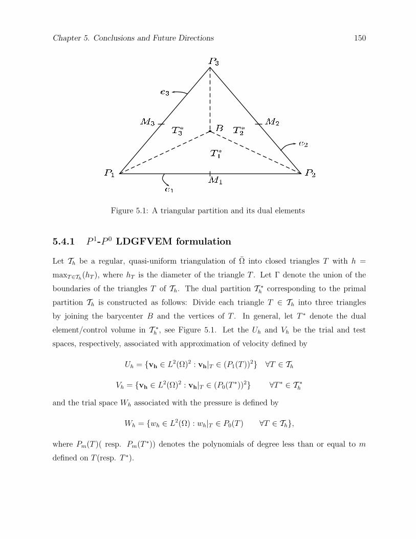
Chapter 5. Conclusions and Future Directions 150
Figure 5.1: A triangular partition and its dual elements
5.4.1 P 1-P 0 LDGFVEM formulation
Let Th be a regular, quasi-uniform triangulation of Ω into closed triangles T with h =
maxT∈Th(hT ), where hT is the diameter of the triangle T . Let Γ denote the union of the
boundaries of the triangles T of Th. The dual partition T ∗h corresponding to the primal
partition Th is constructed as follows: Divide each triangle T ∈ Th into three triangles
by joining the barycenter B and the vertices of T . In general, let T ∗ denote the dual
element/control volume in T ∗h , see Figure 5.1. Let the Uh and Vh be the trial and test
spaces, respectively, associated with approximation of velocity defined by
Uh = vh ∈ L2(Ω)2 : vh|T ∈ (P1(T ))2 ∀T ∈ Th
Vh = vh ∈ L2(Ω)2 : vh|T ∈ (P0(T∗))2 ∀T ∗ ∈ T ∗
h
and the trial space Wh associated with the pressure is defined by
Wh = wh ∈ L2(Ω) : wh|T ∈ P0(T ) ∀T ∈ Th,
where Pm(T )( resp. Pm(T ∗)) denotes the polynomials of degree less than or equal to m
defined on T (resp. T ∗).
Chapter 5. Conclusions and Future Directions 151
Let U(h) = Uh + H2(Ω). For connecting the trial and test spaces, define the transfer
operator γ : V (h) −→ Uh as follows:
γv|T ∗ =1
he
∫
e
v|T ∗ds, T ∗ ∈ T ∗h , (5.4.6)
where e is an edge in T , T ∗ is the dual element in T ∗h containing e and he is the length of
the edge e.
Multiplying (5.4.1) by vh ∈ Vh, integrating over the control volumes T ∗ ∈ T ∗h , applying
Gauss’s divergence theorem and summing up over all the control volumes, we obtain
(K−1u,vh) −∑
T ∗∈T ∗
h
∫
∂T ∗
pvh · nds = 0 ∀vh ∈ Vh, (5.4.7)
where n denotes the outward unit normal vector to the boundary ∂T ∗ of T ∗. Let T ∗j ∈
T ∗h (j = 1, 2, 3) be the three triangles in T ∈ Th, (see Figure 5.1). Then, for wh ∈ Wh
∑
T ∗∈T ∗
h
∫
∂T ∗
pvh · nds =∑
T∈Th
3∑
j=1
∫
∂T ∗
j
pvh · nds
=∑
T∈Th
3∑
j=1
∫
Aj+1BAj
pvh · nds+∑
T∈Th
∫
∂T
pvh · nds. (5.4.8)
In order to rewrite the last term on the right hand side of (5.4.8), we note that for any four
real numbers a, b, c and d, we have
ac− bd =1
2(a + b)(c− d) +
1
2(a− b)(c + d). (5.4.9)
Using (5.4.3), (5.4.9) and the fact that [p] = 0, (5.4.8) becomes
∑
T ∗∈T ∗
h
∫
∂T ∗
pvh · nds =∑
T∈Th
3∑
j=1
∫
Aj+1BAj
pvh · nds+∑
e∈Γ
∫
e
[vh] · 〈p〉ds. (5.4.10)
Now we are in position to define our P 1 − P 0 LDGFVEM:
Find (uh, ph) ∈ Uh ×Wh such that
(uh, γvh) +∑
T∈Th
3∑
j=1
∫
Aj+1BAj
phγvh · nds+∑
e∈Γ
∫
e
ph[γvh]ds = 0 ∀vh ∈ Uh (5.4.11)
(∇.uh) −∑
e∈Γ
∫
e
wh[γuh] = (f, wh) ∀wh ∈ Wh (5.4.12)
Chapter 5. Conclusions and Future Directions 152
where wh are the approximation of wh referred to as numerical flux, on the boundary of a
triangle T ∈ Th.In immediate future, we propose to develop the error estimates for the LDGFVEM applied
to the concentration equation. Note that LDG methods also can be a good choice for
the approximation of the convection-diffusion equations if the numerical fluxes are chosen
suitably, see [12, 30].
5.4.2 Modified methods of characteristics with adjust advection
(MMOCAA) procedure
The modified method of characteristics is not conservative in nature, but a modification
of MMOC called MMOCAA, proposed by Douglas et al. [39] is conservative in nature. It
also has been observed that this new scheme is naturally parallelizable and more accurate
as it reduces the effects of grid orientation, the excessive smoothing of the sharp fronts and
has low storage requirements. As in Chapter 4, the concentration equation can be written
as
ψ(x, t)∂c
∂s−∇ · (D(u)∇c) = (c− c)q ∀(x, t) ∈ Ω × J. (5.4.13)
where ψ(x, t) = (|u(x, t)|2 + φ(x)2)1
2 = (u1(x)2 + u2(x)
2 + φ(x)2)1
2 and s be the unit vector
in the direction of (u1, u2, φ) in Ω × J .
In MMOCAA procedure one splits the concentration equations into two sub equations
namely, advection and transport equations and different time steps can be used for these
equations. Essentially, in the MMOCCA procedure the advection term is treated as a
primary variable and hence, more accurate approximation for the advection is excepted.
Following this procedure, the concentration equation (5.4.13) can be split into a system of
partial differential equations as
v = −D(u)∇c ∀(x, t) ∈ Ω × J, (5.4.14)
ψ(x)∂c
∂s+ ∇ · v = (c− c)q ∀(x, t) ∈ Ω × J, (5.4.15)
It is also noted through experiments in [39] that there are advantages if one considers larger
time step for advection term. We also plan to study MMOCAA for the approximation of the
Chapter 5. Conclusions and Future Directions 153
concentration equation. Since in LDG methods also, we split the second order equations
into two first order equations, it would be good idea to combined LDG methods with
MMOC.
Bibliography
[1] M. Ali, Numerical methods for enhanced oil recovery in reservoir simulation, Ph.D
Thesis, I.I.T. Bombay, 1997.
[2] M. Ali and A. K. Pani, An H1-Galerkin mixed finite element method combined with the
modified method of characteristics for incompressible miscible displacement problems
in porous media., Differential Equations and Dynam. Systems 6 (1998), 135–147.
[3] D. N. Arnold, An interior penalty finite element method with discontinuous elements,
SIAM J. Numer. Anal. 19 (1982), 742–760.
[4] D. N. Arnold, F. Brezzi, B. Cockburn, and L. D. Marini, Unified analysis of dis-
continuous Galerkin methods for elliptic problems, SIAM J. Numer. Anal. 39 (2002),
1749–1779.
[5] I. Babuska, The finite element method with penalty, Math. Comp. 27 (1973), 221–228.
[6] C. Bahriawati and C. Carstensen, Three matlab implementation of the lowest-order
Raviart-Thomas MFEM with a posteriori error control, Comput. Methods Appl. Math.
5 (2005), 333–361.
[7] R. E. Bank and D. J. Rose, Some error estimates for the box method, SIAM J. Numer.
Anal. 24 (1987), 777–787.
[8] S. C. Brenner and L. R. Scott, The mathematical theory of finite element methods,
Springer-Verlag, New York, 1994.
154
BIBLIOGRAPHY 155
[9] F. Brezzi and M. Fortin, Mixed and hybrid finite element methods, Springer -Verlag,
New York, 1991.
[10] Z. Cai, On the finite volume element method, Numer. Math. 58 (1991), 713–735.
[11] P. Castillo, B. Cockburn, I. Perugia, and D. Schotzau, An a priori error analysis of
the local discontinuous Galerkin method for elliptic problems, SIAM J. Numer. Anal.
38 (2000), 1676–1706.
[12] P. Castillo, B. Cockburn, D. Schotzau, and C. Schwab, Optimal a priori error estimates
for the hp-version of the local discontinuous Galerkin method for convection-diffusion
problems., Math. Comp. 71 (2002), 455–478.
[13] S. Champier, T. Gallouet, and R. Herbin, Convergence of an upstream finite volume
scheme for a nonlinear hyperbolic equation on a triangular mesh, Numer. Math. 66
(1993), 139–157.
[14] P. Chatzipantelidis, A finite volume method based on the Crouzeix-Raviart element for
elliptic PDE’s in two dimensions, Numer. Math. 82 (1999), 409–432.
[15] , Finite volume methods for elliptic PDE’s: A new approach, M2AN Math.
Model. Numer. Anal. 36 (2002), 307–324.
[16] P. Chatzipantelidis, V. Ginting, and R. D. Lazarov, A finite volume element method
for a nonlinear elliptic problem, Numer. Linear Algebra Appl. 12 (2005), 515–546.
[17] P. Chatzipantelidis, R. D. Lazarov, and V. Thomee, Error estimates for a finite volume
element method for parabolic equations in convex polygonal domains, Numer. Methods
Partial Differential Equations 20 (2004), 650–674.
[18] G. Chavent and J. Jaffre, Mathematical models and finite elements for reservoir sim-
ulation, Elsevier, Amsterdam, 1986.
BIBLIOGRAPHY 156
[19] Z. Chen, Finite element methods and their applications, Springer-Verlag, New York,
2005.
[20] Z. Chen and R. E. Ewing, Mathematical analysis for reservoir models, SIAM J. Math.
Anal. 30 (1999), 431–453.
[21] C. Choquet, On a fully coupled nonlinear parabolic problem modelling miscible dis-
placement in porous media, J. Math. Anal. Appl. 339 (2008), 1112–1133.
[22] S. H. Chou, Analysis and convergence of a covolume method for the generalized Stokes
problem, Math. Comp. 66 (1997), 85–104.
[23] S. H. Chou and D. Y. Kwak, Mixed covolume methods on rectangular grids for elliptic
problems., SIAM J. Numer. Anal. 37 (2000), 758–771.
[24] S. H. Chou, D. Y. Kwak, and K. Y. Kim, Mixed finite volume methods on nonstaggered
quadrilateral grids for elliptic problems, Math. Comp. 72 (2002), 525–539.
[25] S. H. Chou, D. Y. Kwak, and Q. Li, Lp error estimates and superconvergence for covol-
ume or finite volume element methods, Numer. Methods Partial Differential Equations
19 (2003), 463–486.
[26] S. H. Chou, D. Y. Kwak, and P. S. Vassilevski, Mixed covolume methods for elliptic
problems on triangular grids, SIAM J. Numer. Anal. 35 (1998), 1850–1861.
[27] S. H. Chou and Q. Li, Error estimates in L2, H1 and L∞ in covolume methods for
elliptic and parabolic problems: A unified approach, Math. Comp. 69 (2000), 103–120.
[28] S. H. Chou and X. Ye, Unified analysis of finite volume methods for second order
elliptic problems, SIAM J. Numer. Anal. 45 (2007), 1639–1653.
[29] P. G. Ciarlet, The finite element method for elliptic problems, North-Holland, New
York, 1978.
BIBLIOGRAPHY 157
[30] B. Cockburn and C. Shu, The local discontinuous Galerkin method for time-dependent
convection-diffusion systems, SIAM J. Numer. Anal. 35 (1998), 2440–2463.
[31] B. L. Darlow, R. E. Ewing, and M. F. Wheeler, Mixed finite element methods for
miscible displacement in porous media, SPEJ 24 (1984), 391–398.
[32] P. C. Das and A. K. Pani, C0- interior penalty Galerkin procedures for slightly com-
pressible miscible displacement in porous media, Proc. International conference on non-
linear mechanics, Shanghai, China, Oct, 28-31, 1985, Chien WeiZang (Ed.), Sciences
Press, Beijing, 1985, pp. 1186–1191.
[33] C. Dawson, P k+1−Sk local discontinuous Galerkin method for elliptic equations, SIAM
J. Numer. Anal. 40 (2002), 2151–2170.
[34] C. N. Dawson, T. F. Russell, and M. F. Wheeler, Some improved error estimates for
the modified method of characteristics, SIAM J. Numer. Anal. 26 (1989), 1487–1512.
[35] J. Douglas, Jr., and T. Dupont, Interior penalty procedures for elliptic and parabolic
Galerkin methods, in Computing Methods in Applied Sciences, Lecture notes in
Physics, 58, Springer-Verlag, Berlin, 1976, pp. 207–216.
[36] J. Douglas, Jr., T. Dupont, and R. E. Ewing, Incomplete iteration for time-stepping
a Galerkin method for a quasilinear parabolic problem, SIAM J. Numer. Anal. 16
(1979), 503–522.
[37] J. Douglas, Jr., R. E. Ewing, and M. F. Wheeler, The approximation of the pressure
by a mixed method in the simulation of miscible displacement, RAIRO Anal. Numer.
17 (1983), 17–33.
[38] , A time-discretization procedure for a mixed finite element approximation of
miscible displacement in porous media, RAIRO Anal. Numer. 17 (1983), 249–265.
[39] J. Douglas, Jr., F. Frederico, and P. Felipe, On the numerical simulation of water-
flooding of heterogeneous petroleum reservoirs, Comput. Geosci. 1 (1997), 155–190.
BIBLIOGRAPHY 158
[40] J. Douglas, Jr., M. F. Wheeler, B. L. Darlow, and R. P. Kendall, Self-adaptive finite
element simulation of miscible displacement in porous media, Comput. Meth. Appl.
mech. Engrg. 47 (1984), 131–159.
[41] Jim Douglas, Jr., and T. F. Russell, Numerical methods for convection-dominated
diffusion problems based on combining the method of characteristics with finite element
method or finite difference procedures, SIAM J. Numer. Anal. 19 (1982), 871–885.
[42] R. G. Duran, On the approximation of miscible displacement in porous media by a
method characteristics combined with a mixed method, SIAM J. Numer. Anal. 25
(1988), 989–1001.
[43] L. C. Evans, Partial differential equations, graduate studies in mathematics, American
Mathematical society, Rhode Island, 1998.
[44] R. E. Ewing, , T. F. Russell, and M. F. Wheeler, Convergence analysis of an ap-
proximation of miscible displacement in porous media by mixed finite elements and
a modified method of characteristics, Comput. Meth. Appl. mech. Engrg. 47 (1984),
73–92.
[45] R. E. Ewing, R. D. Lazarov, and Y. Lin, Finite volume element approximations of
nonlocal reactive flows in porous media, Numer. Methods Partial Differential Equations
16 (2000), 285–311.
[46] R. E. Ewing, T. Lin, and Y. Lin, On the accuracy of the finite volume element method
based on piecewise linear polynomials, SIAM J. Numer. Anal. 39 (2002), 1865–1888.
[47] R. E. Ewing and T. F. Russell, Efficient time-stepping methods for miscible displace-
ment problems in porous media, SIAM J. Numer. Anal. 19 (1982), 1–67.
[48] R. E. Ewing and M. F. Wheeler, Galerkin methods for miscible displacement problems
in porous media, SIAM J. Numer. Anal. 17 (1980), 351–365.
BIBLIOGRAPHY 159
[49] X. Feng, On existence and uniqueness results for a coupled system modeling miscible
displacement in porous media., J. Math. Anal. Appl. 194 (1995), 883–910.
[50] P. Houston, C. Schwab, and E. Suli, Discontinuous hp-finite element methods for
advection-diffusion-reaction problems, SIAM J. Numer. Anal. 39 (2002), 2133–2163.
[51] H. Jianguo and X. Shitong, On the finite volume element method for general self-
adjoint elliptic problems, SIAM J. Numer. Anal. 35 (1998), 1762–1774.
[52] S. Kesawan, Topics in functional analysis and applications, Wiley-Eastern Ltd., New
Delhi, 1989.
[53] K. Y. Kim, Mixed finite volume method for nonlinear elliptic problems, Numer. Meth-
ods Partial Differential Equations 21 (2005), 791–809.
[54] G. Kossioris, Ch. Makridakis, and P. E. Souganidis, Finite volume schemes for
Hamilton-Jacobi equations, Numer. Math. 83 (1999), 427–442.
[55] S. Kumar, N. Nataraj, and A. K. Pani, Discontinuous Galerkin finite volume ele-
ment methods for second order linear elliptic problems, Submitted to Numer. Methods
Partial Differential Equations.
[56] , Finite volume element method for second order hyperbolic equations, Inl. J.
Numer. Anal. and Model. 5 (2008), 132–151.
[57] D. Y. Kwak and K. Y. Kim, Mixed covolume methods for quasi-linear second-order
elliptic problems, SIAM J. Numer. Anal. 38 (2000), 1057–1072.
[58] Y. Kwon and F. A. Milner, L∞-error estimates for mixed methods for semilinear
second-order elliptic equations, SIAM J. Numer. Anal. 25 (1988), 46–53.
[59] R. H. Li, Generalized difference methods for a nonlinear Dirichlet problem, SIAM J.
Numer. Anal. 24 (1987), 77–88.
BIBLIOGRAPHY 160
[60] R. H. Li, Z. Y. Chen, and W. Wu, Generalized difference methods for differential
equations, Marcel Dekker, New York, 2000.
[61] N. Mangiavacchi, A. Castelo, M. F. Tome, J. A. Cuminato, M. L. B. de Oliveira, and
S. McKee, An effective implementation of surface tension using the marker and cell
method for axisymmetric and planar flows, SIAM J. Sci. Comput. 26 (2005), 1340–
1368.
[62] T. McCracken and J. Yanosik, A nine-point finite difference reservoir simulation for
realistic prediction of adverse mobility ratio displacement, SPEJ 19 (1979), 253–262.
[63] F. A. Milner, Mixed finite element methods for quasilinear second-order elliptic prob-
lems, Math. Comp. 44 (1985), 303–320.
[64] I. D. Mishev, Finite volume and finite volume element methods for non-symmetric
problems, Ph.D Thesis, Technical Report ISC-96-04-MATH, Institute of Scientific
Computation, Texas A&M University, College Station, TX, 1997.
[65] A. K. Pani, V. V. Thomee, and L. B. Wahlbin, Numerical methods for hyperbolic
and parabolic integro-differential equations, J. Integral Equations and Appl. 4 (1992),
533–584.
[66] D. W. Peaceman, Improved treatment of dispersion in numerical calculations of mul-
tidimensional miscible displacement, SPEJ 6 (1966), 213–216.
[67] , Fundamentals of numerical reservoir simulation, Elsevier, Amsterdam, 1977.
[68] S. Prodhomme, F. Pascal, J. T. Oden, and A. Romkes, Review of error estimation of
discontinuous Galerkin methods, TICAM REPORT 00-27, October 17, 2000.
[69] Rama Mohana Rao, M., Ordinary differential equations theory and applications, East-
West Press Pvt. Ltd., New Delhi, 1980.
BIBLIOGRAPHY 161
[70] B. Riviere, M. F. Wheeler, and V. Girault, A priori error estimates for finite element
methods based on discontinuous approximation spaces for elliptic problems, SIAM J.
Numer. Anal. 39 (2001), 902–931.
[71] G. E. Robertson and P. T. Woo, Grid orientation effects and the use of orthogonal
curvilinear coordinates in reservoir simulation, SPEJ 18 (1978), 13–19.
[72] T. F. Russell, An incompletely iterated characteristic finite element method for a mis-
cible displacement problem, Ph.D. Thesis, Univ. Chicago, Illinois, 1980.
[73] T. F. Russell and M. F. Wheeler, Finite element and finite difference methods for
continuous flows in porous media, The Mathematics of reservoir simulation, R. E.
Ewing (ed.), SIAM, Philadelphia (1983), 35–107.
[74] P. H. Sammon, Numerical approximations for a miscible displacement process in porous
media., SIAM J. Numer. Anal. 23 (1986), 508–542.
[75] R. K. Sinha, R. E. Ewing, and R. D. Lazarov, Some new error estimates of a semidis-
crete finite volume element method for a parabolic intgro-differential equation with
nonsmooth initial data, SIAM J. Numer. Anal. 43 (2006), 2320–2343.
[76] S. Sun, B. Riviere, and M. F. Wheeler, A combined mixed finite element and discon-
tinuous Galerkin method for miscible displacement problem in porous media, Recent
progress in Computational and Applied PDEs, Conference Proceedings for the Inter-
national Conference Held in Zhangjiaje, 2001, pp. 321–348.
[77] S. Sun and M. F. Wheeler, Symmetric and nonsymmetric discontinuous Galerkin meth-
ods for reactive transport in porous media, SIAM J. Numer. Anal. 43 (2005), 195–219.
[78] V. Thomee, Galerkin finite element methods for parabolic problems, Springer-Verlag,
New York, 1984.
[79] M. R. Todd, P. M. O’Dell, and G. J. Hirasaki, Methods for increased accuracy in
numerical simulation, SPEJ 12 (1972), 515–530.
BIBLIOGRAPHY 162
[80] H. Wang, D. Liang, R. E. Ewing, S. L. Lyons, and G. Qin, An approximation to miscible
fluid flows in porous media with point sources and sinks by an Eulerian-Lagrangian
localized adjoint method and mixed finite element methods, SIAM J. Sci. Comput. 22
(2000), 561–581.
[81] T. Wang, A mixed finite volume element method based on rectangular mesh for bihar-
monic equations, J. Comput. Appl. Math. 172 (2004), 117–130.
[82] M. F. Wheeler, An elliptic collocation-finite element method with interior penalties,
SIAM J. Numer. Anal. 15 (1978), 152–161.
[83] M. F. Wheeler and B. L. Darlow, Interior penalty Galerkin procedures for miscible dis-
placement problems in porous media, Computational Methods in Nonlinear Mechanics,
J. T. Oden (ed.), North-Holand (1980), 485–506.
[84] D. Q. Yang, Mixed methods with dynamic finite element spaces for miscible displace-
ment in porous media, J. Comput. Appl. Math. 30 (1990), 313–328.
[85] Xiu Ye, A new discontinuous finite volume method for elliptic problems, SIAM J.
Numer. Anal. 42 (2004), 1062–1072.
[86] , A discontinuous finite volume method for the Stokes problems, SIAM J. Nu-
mer. Anal. 44 (2006), 183–198.

Acknowledgments
It is a great pleasure to take this opportunity to acknowledge the people who have supported
me during the period of research.
First and foremost, I would like to express my heartiest gratitude to my supervisor Prof.
Neela Nataraj for her enthusiastic supervision and kind support. Her detailed and con-
structive lectures on ’MATLAB implementations for finite element methods’, have helped
me a lot in understanding the basics of numerical implementations. This understanding
really helped me in developing implementation procedure for my research problems. I really
learned a lot of mathematics by attending some of her talks and lectures.
Secondly, I am deeply grateful to my co-supervisor Prof. Amiya K. Pani for giving me
invaluable suggestions throughout this research. I express my heart-full thanks to him for
suggesting me the model problem and introducing the field of finite element methods. I
cannot imagine to have completed this research work without his intuitive suggestions and
excellent lectures. I owe a lot of gratitude to him for showing me the way of research. I am
also very thankful to his wife Mrs. Tapaswani Pani for her support.
I am greatly thankful to my RPC (Research Progress Committee) members: Prof. Rekha
P. Kulkarni and Prof. K. Suresh Kumar for their valuable suggestions and comments.
I am very thankful to the Department of Mathematics, IIT Bombay for providing me the
working place and computing facility during my research work.
I acknowledge the National Board for Higher Mathematics for providing me with financial
support to attend some international conferences abroad.
Many thanks to my parents Shri Mool Chand and Smt. Beena Devi, who taught me the
value of hard work by their own example. I am also grateful to my younger brother Mr.
Pravesh Kumar for his encouragement and moral support to continue my studies and in
taking care of my family in my absence at my village Bahadarpur.
Thanks to my dear friends and colleagues for their help and also for creating a homely

environment at IIT Bombay. My special thanks goes to Sangita Yadav who really helped
me in Matlab implementation. I am also thankful to my senior Dr. Tirupathi Gudi for his
valuable discussions.
Finally, I would like to thank all whose direct and indirect support helped me in completing
my thesis.
IIT Bombay Sarvesh Kumar
Recommended