CER
N-T
HES
IS-2
013-
036
16/0
5/20
13
DEPARTMENT OF MECHANICAL ENGINEERING
FINITE ELEMENT MODELLING OF X-BAND RF FLANGES
Lauri Kortelainen
BACHELOR’S THESIS
2013
Supervisors: Dr. Hannu Koivurova
Dr. Germana Riddone

ABSTRACT
Finite element modelling of x-band RF flanges
Lauri Kortelainen
University of Oulu, Department of Mechanical Engineering
Bachelor’s thesis 2013, 48 p. + 2 p. appendixes
Supervisor(s): Dr. Hannu Koivurova
Dr. Germana Riddone
A finite element model of different versions of RF flange used in Compact Linear
Collider modules was created in ANSYS Workbench software. A 2D idealisation of the
assembly was modelled using both plane stress and plane strain elements. Three of the
versions were also modelled using 3D elements. A detailed description of finite element
models and theoretical background accompanying the models are presented in this
thesis.
Keywords: CERN, FEA, RF, FLANGE

TIIVISTELMÄ
Finite element modelling of x-band RF flanges
Lauri Kortelainen
Oulun yliopisto, Konetekniikan osasto
Kandidaatintyö 2013, 48 s. + 2 s. liitteitä
Työn ohjaaja(t): TkT Hannu Koivurova
Dr. Germana Riddone (CERN)
Compact Linear Collider –moduuleissa sijaitsevan laippakokoonpanon eri versiot
mallinnettiin käyttäen elementtimenetelmää ANSYS Workbench –ohjelmistolla.
Kokoonpano mallinnettiin käyttäen kaksiulotteisia tasojännitys ja –venymäelementtejä.
Kolme versioista mallinnettiin myös käyttäen kolmiulotteisia solidielementtejä. Tämä
työ esittelee mallinnuksen yksityiskohdat ja teoriaa liittyen aiheeseen.
Asiasanat: CERN, FEA, RF, FLANGE
ACKNOWLEDGEMENT
This thesis was carried out at CERN in a collaboration with Helsinki Institute of Physics
(HIP) and University of Oulu. I would like to thank my supervisors Dr. Hannu
Koivurova and Dr. Germana Riddone for their guidance and support. I also thank Dr.
Fabrizio Rossi for giving me technical advice during the development of the simulation.
Geneva, 16th of April 2013
Lauri Kortelainen

TABLE OF CONTENTS
ABSTRACT
TIIVISTELMÄ
ACKNOWLEDGEMENT
TABLE OF CONTENTS
NOTATIONS
ABBREVIATIONS
1 INTRODUCTION............................................................................................................... 7
1.1 Background .................................................................................................................. 8
1.2 CLIC study ................................................................................................................... 9
2 THEORETICAL BACKGROUND .................................................................................. 12
2.1 Tensile tests ................................................................................................................ 12
2.1.1 Behaviour at larger strains ................................................................................ 15
2.1.2 True stress and strain ........................................................................................ 16
2.2 Material models .......................................................................................................... 18
2.2.1 Linear elastic ..................................................................................................... 18
2.2.2 Nonlinear elastic-plastic material model .......................................................... 20
2.3 2D idealisation ........................................................................................................... 22
2.4 Influence of heat treatment on mechanical properties of material: annealing ........... 24
3 TECHNICAL DESCRIPTION OF THE X-BAND RF FLANGE ................................... 25
3.1 Geometry .................................................................................................................... 25
4 2D FINITE ELEMENT MODEL DESCRIPTION .......................................................... 26
4.1 Model ......................................................................................................................... 26
4.2 Material ...................................................................................................................... 28
4.3 Mesh ........................................................................................................................... 29
4.4 Contact modelling ...................................................................................................... 30
4.5 Boundary conditions .................................................................................................. 31
5 3D FINITE ELEMENT MODEL DESCRIPTION .......................................................... 33
5.1 Model ......................................................................................................................... 33
5.2 Material ...................................................................................................................... 34
5.3 Mesh ........................................................................................................................... 34
5.4 Contact modelling ...................................................................................................... 34
5.5 Boundary conditions .................................................................................................. 35

6 RESULTS ......................................................................................................................... 37
6.1.1 2D plane stress and strain modelling ................................................................ 37
6.1.2 3D modelling .................................................................................................... 39
7 CONCLUSIONS AND FUTURE STEPS ........................................................................ 46
8 REFERENCES .................................................................................................................. 47
APPENDIX 1
NOTATIONS
A cross-sectional area
E Young’s Modulus
Et tangent modulus
F force
ε engineering strain
εt true strain
υ Poisson’s ratio
Δl elongation
σ engineering stress
σt true stress

ABBREVIATIONS
CLIC Compact Linear Collider
ILC International Linear Collider
LEP Large Electron-Positron Collider
LHC Large Hadron Collider
AS Accelerating Structure
PETS Power Extraction and Transfer Structure
RF Radio Frequency
MB Main Beam
DB Drive Beam
FEA Finite Element Analysis

7
1 INTRODUCTION
This thesis presents the finite element modelling of x-band RF flange used in CLIC
modules. The aim of the finite element modelling is to examine the deformations of the
copper gasket for different versions of the flange and to check if the specified
requirements are met. In addition to the detailed description of the numerical
simulations, the theoretical background is presented. The theoretical part of the thesis
includes information about tensile tests and how the data obtained from them can be
implemented in the finite element modelling. Elastic-plastic material models are
described as well and the theory behind the two-dimensional idealisation of three-
dimensional structure is presented.
Chapter 1 introduces CERN, CLIC project and CLIC two-beam modules. The
theoretical background for the simulation is presented in chapter 2. Chapter 3 presents
the flange assembly in question and its technical specifications. Chapter 4 describes the
two-dimensional finite element model, whereas chapter 5 describes the three-
dimensional one. Results of the simulations are presented in chapter 6. Chapter 7
includes conclusions and future steps.

8
1.1 Background
The European Organization for Nuclear Research (CERN), one of the world’s largest
and most respected particle physics laboratory, was founded in 1954. Today CERN is
run by 20 Member States but also many non-European countries are involved in
different research programs. (Ellis 2000.) Currently about 2400 people are employed by
CERN but over 10 000 visiting scientists are related to the on-going projects through
their research. They represent 608 universities and 113 nationalities. (About CERN
2013.)
CERN’s main function is to provide accelerators for the high-energy physics research.
During CERN’s existence, several important scientific discoveries have been made in
physics. Furthermore, the research work related to particle accelerator studies has
revolutionized the technology used in many other fields. For example, CERN had an
important role in the discovery of Positron Emission Tomography (PET) technology,
which enables three-dimensional imaging of the functional processes of the brain.
Recently, CERN has been a centre for the development of the grid network which
enables the handling of large amounts of data produced by the current accelerator
projects. (Physics for Health 2010.)
At the moment, LHC (Large Hadron Collider), which was completed in 2008, is
CERN’s most important accelerator. The circular LHC tunnel, which was occupied by
LEP (Large Electron-Positron Collider) until year 2000, has a circumference of 27 km
and is located 100 meters underground. On the 4th of July 2012 CERN held a press
conference in which the finding of a new gauge boson was confirmed. As of February
2013 the operation of LHC was interrupted for LS1 (Long Shutdown 1). During
shutdown wear parts will be replaced and upgrades will be made.
Many of the open questions in physics can be best addressed by a lepton-antilepton
(electron-positron collider) instead of a hadron collider like LHC. A consensus has been
reached among particle physicists that the results from the LHC have to be
complemented by experiments at an electron-positron collider operating in the TeV
9
energy range. (Ellis 2000: 3.) Today, two approaches as a future linear collider are
being developed in parallel: International Linear Collider (ILC) and Compact Linear
Collider (CLIC). They have a different energy range, which leads to a different choice
of technology. The main difference between the two is that ILC uses superconducting
technology like LHC, which means components must be close to the absolute zero
temperature, while CLIC uses normal-conducting technology at temperatures close to
room temperature. (Geschonke 2010.)
1.2 CLIC study
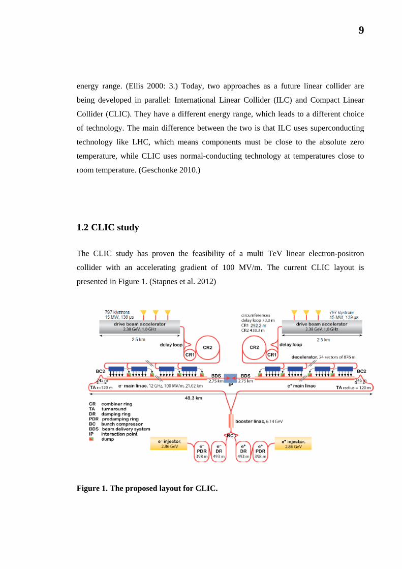
The CLIC study has proven the feasibility of a multi TeV linear electron-positron
collider with an accelerating gradient of 100 MV/m. The current CLIC layout is
presented in Figure 1. (Stapnes et al. 2012)
Figure 1. The proposed layout for CLIC.

10
The layout of CLIC relies on transforming the high current intensity and low energy
from the Drive Beam (DB) to the low current and high energy Main Beam (MB). The
RF power created in Power Extraction and Transfer Structures (PETS) is transferred
through RF network to the Accelerating Structures (AS). The beam focusing is achieved
by using quadrupole magnets which are situated along the whole length of the linac.
The concept of the accelerator with the main components such as AS, PETS and
quadrupoles can be seen in Figure 2. (Stapnes et al. 2012)
Figure 2. The CLIC Two-Beam scheme. The power provided by PETS is
transferred to AS through RF network.
The CLIC main linacs consist of a series of two-beam modules each having a length of
about 2 metres. The main components of a module are Accelerating Structures (AS) and
Power-Extraction and Transfer Structures (PETS). A 3D model of a two-beam module
is shown in Figure 3.

11
Figure 3. CLIC Two-Beam Module typical configuration.

12
2 THEORETICAL BACKGROUND
This chapter presents theoretical background for the finite element simulations.
2.1 Tensile tests
The aim of a tensile test is to evaluate material properties for the metal in question. The
properties obtained can then be used for the design of components. For the tensile test
first the specimen is placed in the testing machine (Figure 4) and then a force is applied.
The force is increased very slowly and a strain gauge measures the change of length in
the specimen. The results of a single test can then be applied to all sizes and cross-
sections of specimens if the force is converted to stress and the distance between gauge
marks to strain. Engineering stress and strain are defined in equations (1) and (2).
(Askeland et al. 2010: 159-161.)
Figure 4. Uniaxial testing machine for tensile test.

13
(1)
where, σ
F
A0
engineering stress [Pa]
force [N]
initial cross-sectional area [m2]
(2)
where, ε
engineering strain
elongation [m]
initial length of the test specimen [m]
Figure 5 presents a typical stress-strain curve at small strains obtained from a tensile
test. The highest stress that can be applied in the linear region is called the
proportional limit. The maximum stress that can be applied without causing permanent
deformations is called the elastic limit. Usually the value found from reference books
of material properties is neither of these. The departure from elasticity is defined by
means of proof stress, value which is independent of the accuracy of the measurement
device. This is done by choosing a strain value (normally 0.2%) and drawing a line
parallel to Young’s modulus at this point. The point of intersection between this line
and the stress-strain curve marks the proof stress. This procedure also known as the
offset method is shown in Figure 6. (Martin 2006: 37-38.)

14
Figure 5. Behaviour of metal at small strains.
Figure 6. The offset method for evaluating the proof stress.
15
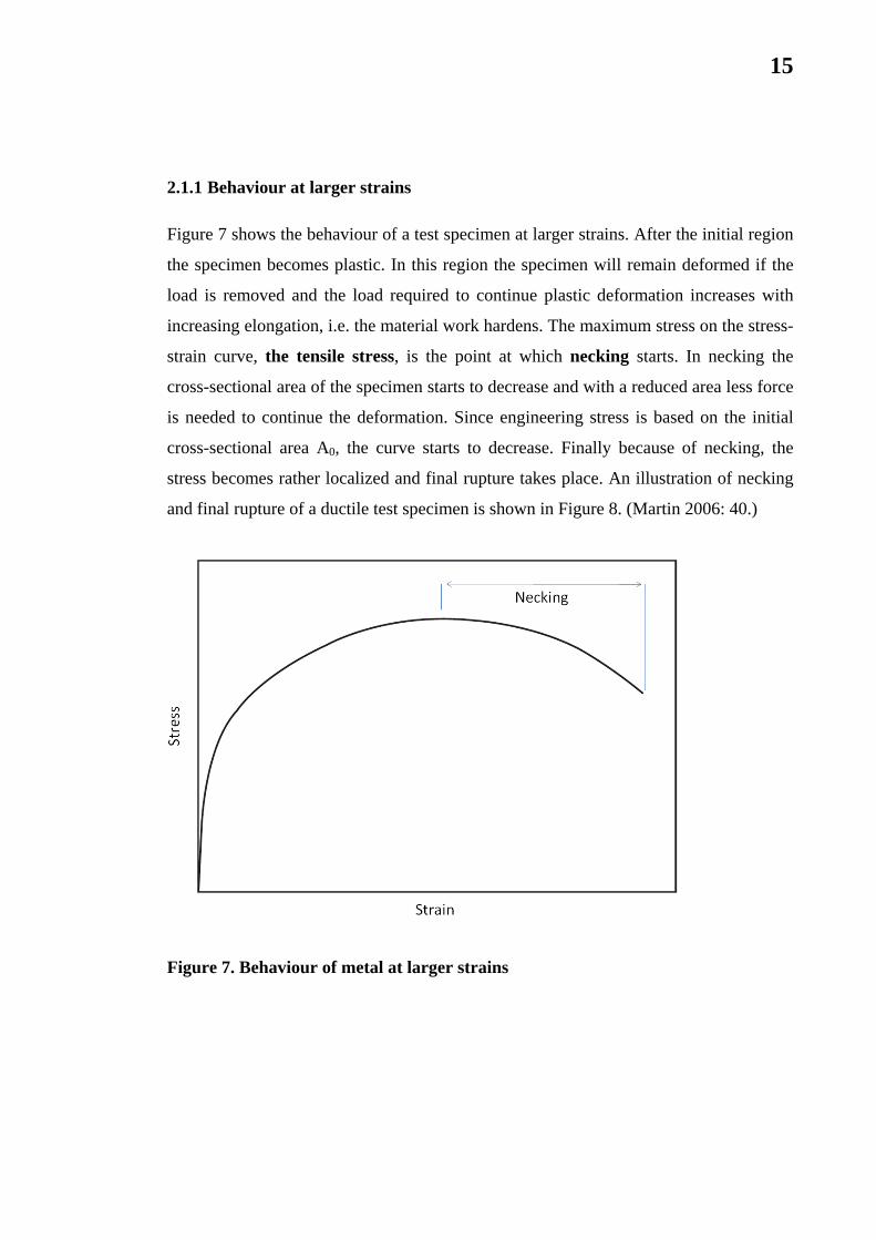
2.1.1 Behaviour at larger strains
Figure 7 shows the behaviour of a test specimen at larger strains. After the initial region
the specimen becomes plastic. In this region the specimen will remain deformed if the
load is removed and the load required to continue plastic deformation increases with
increasing elongation, i.e. the material work hardens. The maximum stress on the stress-
strain curve, the tensile stress, is the point at which necking starts. In necking the
cross-sectional area of the specimen starts to decrease and with a reduced area less force
is needed to continue the deformation. Since engineering stress is based on the initial
cross-sectional area A0, the curve starts to decrease. Finally because of necking, the
stress becomes rather localized and final rupture takes place. An illustration of necking
and final rupture of a ductile test specimen is shown in Figure 8. (Martin 2006: 40.)
Figure 7. Behaviour of metal at larger strains

16
Figure 8. Necking (a) and final rupture (b) of a ductile test specimen.
2.1.2 True stress and strain
Engineering stress is defined by using the initial cross-sectional area A0, which leads to
the decrease in engineering stress at the onset of necking. In reality the cross-sectional
area changes continually. True stress is defined by using the deformed cross-section
instead of the initial one. True strain, also known as the logarithmic strain, provides the
correct measure of the strain when deformation occurs incrementally, taking into
account the influence of the strain path. Equations (3) and (4) define true stress and true
strain while equations (5) and (6) show the relationships between engineering and true
stress, and engineering and true strain respectively. Equations (5) and (6) are only valid
until the onset of necking. Beyond this point true stress and strain should be computed
from actual load, cross-sectional area and gauge length parameters. (Callister 2001:
167-168; Smallman 1999: 197-199.)

17
(3)
where,
F
A
true stress [Pa]
force [N]
cross-sectional area [m2]
ln ln
(4)
where,
true strain
1 (5)
1 (6)
The true stress-strain curve is compared with the engineering stress-strain curve in
Figure 9. The curves are identical until the yield point. After this, true stress continues
to increase. Although the required load decreases, the cross-sectional area decreases
even more leading to increase in stress. (Beer et al 2012: 61-62.)

18
Figure 9. True stress-strain and engineering stress-strain curves.
2.2 Material models
2.2.1 Linear elastic
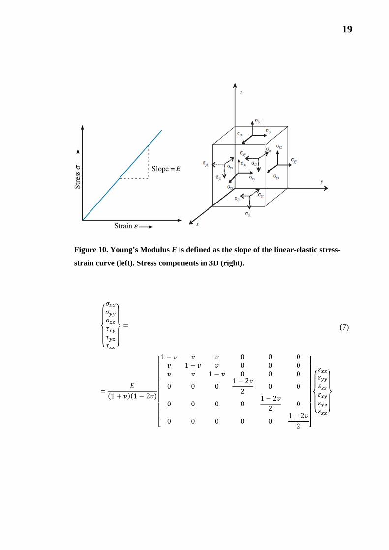
Figure 10 presents the stress-strain curve of a linear elastic material under uniaxial load
and the stress components in 3D. Most engineering structures are designed to undergo
only small deformations, involving only the linear part of the stress-strain curve, in
which the slope of the curve is called Young’s Modulus E. The relationship between
stress and strain components applied in three dimensions, shown in equation (7), is
called the generalized Hooke’s law. (Beer et al 2012: 62.)
19
Figure 10. Young’s Modulus E is defined as the slope of the linear-elastic stress-
strain curve (left). Stress components in 3D (right).
1 1 2
1 0 0 01 0 0 0
1 0 0 0
0 0 01 22
0 0
0 0 0 01 22
0
0 0 0 0 01 22
(7)
20
where,
ε
E
υ
stress component
strain component
Young’s Modulus
Poisson’s Ratio
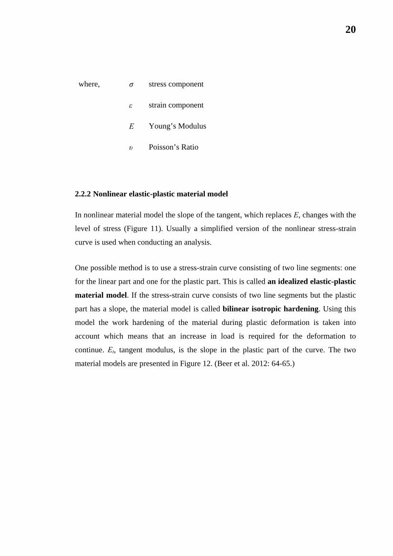
2.2.2 Nonlinear elastic-plastic material model
In nonlinear material model the slope of the tangent, which replaces E, changes with the
level of stress (Figure 11). Usually a simplified version of the nonlinear stress-strain
curve is used when conducting an analysis.
One possible method is to use a stress-strain curve consisting of two line segments: one
for the linear part and one for the plastic part. This is called an idealized elastic-plastic
material model. If the stress-strain curve consists of two line segments but the plastic
part has a slope, the material model is called bilinear isotropic hardening. Using this
model the work hardening of the material during plastic deformation is taken into
account which means that an increase in load is required for the deformation to
continue. Et, tangent modulus, is the slope in the plastic part of the curve. The two
material models are presented in Figure 12. (Beer et al. 2012: 64-65.)

21
Figure 11. Nonlinear stress-strain curve.
Figure 12. An idealized elastic-plastic material model (left) and bilinear hardening
material model (right). E is Young’s Modulus and Et tangent modulus.
22
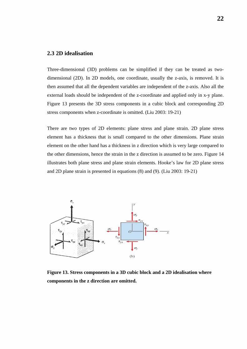
2.3 2D idealisation
Three-dimensional (3D) problems can be simplified if they can be treated as two-
dimensional (2D). In 2D models, one coordinate, usually the z-axis, is removed. It is
then assumed that all the dependent variables are independent of the z-axis. Also all the
external loads should be independent of the z-coordinate and applied only in x-y plane.
Figure 13 presents the 3D stress components in a cubic block and corresponding 2D
stress components when z-coordinate is omitted. (Liu 2003: 19-21)
There are two types of 2D elements: plane stress and plane strain. 2D plane stress
element has a thickness that is small compared to the other dimensions. Plane strain
element on the other hand has a thickness in z direction which is very large compared to
the other dimensions, hence the strain in the z direction is assumed to be zero. Figure 14
illustrates both plane stress and plane strain elements. Hooke’s law for 2D plane stress
and 2D plane strain is presented in equations (8) and (9). (Liu 2003: 19-21)
Figure 13. Stress components in a 3D cubic block and a 2D idealisation where
components in the z direction are omitted.

23
Figure 14. Illustration of plane stress (thin body) and plane strain (thick body)
solids.
1
1 01 0
0 012
(8)
11 1 2
11
0
11 0
0 01 22 1
(9)

24
2.4 Influence of heat treatment on mechanical properties of material: annealing
Annealing is a heat treatment in which a material is exposed to an elevated temperature
and then cooled. This process leads to the elimination of the residual stresses produced
during cold working. Annealing at low temperatures will eliminate the residual stresses
that were produced during cold working without affecting the mechanical properties of
the part. Cold working annealing cycle can be repeated many times to produce the
required material properties. Normally a fine-grained microstructure is desired so the
heat treatment is stopped before appreciable grain growth has occurred. Temperatures
commonly used for annealing cold-worked oxygen free copper are between 250 and 650
°C. (Callister 2001: 124.)

25
3 TECHNICAL DESCRIPTION OF THE X-BAND RF FLANGE
3.1 Geometry
Figure 15 presents the geometry of the flange assembly with the main dimensions. The
assembly consists of two stainless steel flanges and an annealed copper gasket between
them. In order to assure the leak tightness, the two flanges are pushed against each other
by threading the eight screws connecting them. As a result, the copper gasket is
compressed by the axial forces produced by the tightening torque (~8 Nm).
Figure 15. Assembly of RF flanges and the copper gasket (all dimensions are in
millimetres).

26
4 2D FINITE ELEMENT MODEL DESCRIPTION
2D finite element modelling is described in detail in this chapter.
4.1 Model
2D analyses using plane stress and plane strain elements were created in ANSYS
Workbench FEA software to evaluate the deformations of the gasket when compressed
by the two flanges. Figure 16 presents the dimensions of the geometry, the flange knife
being on the left. Twelve different geometries summarized in Table 1 were simulated.
Detailed drawings of the flange and the gasket can be found in Appendix 1. Large
deformation option was enabled to take into account large strains occurring in the
gasket.
Figure 16. 2D model of the flange with gasket.

27
Table 1. Flange geometry parameters for versions 1 to 12.
Version a (mm) b (mm)
1 0.75 0.35
2 0.75 0.3
3 0.5 0.35
4 0.5 0.3
5 1 0.35
6 1 0.3
7 0.5 0.4
8 0.5 0.25
9 0.75 0.4
10 0.75 0.25
11 1 0.4
12 1 0.25

28
4.2 Material
Stainless steel flange was modelled as a linear elastic material. Table 2 shows the
material parameters used for stainless steel.
Table 2. Material properties of stainless steel.
Property Value
Modulus of Elasticity 206 GPa
Poisson’s Ratio 0.3
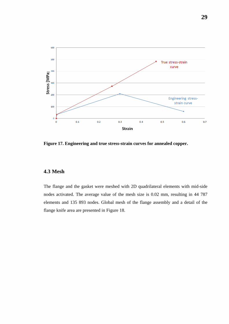
Annealed copper gasket was modelled with a linear-plastic material model. The data
from the material database MatWeb, shown in Table 3, were used to create a bilinear
elastic-plastic engineering stress-strain curve which was further converted to equivalent
true stress-strain curve to model the real behaviour of the material (Figure 17).
Table 3. Material properties of annealed copper.
Property Value
Hardness 50 HV
Tensile Strength, Ultimate 210 MPa
Tensile Strength, Yield 33.3 MPa
Elongation at Break 60 %
Modulus of Elasticity 110 GPa
Bulk Modulus 140 GPa
Poisson’s Ratio 0.343
Shear Modulus 46 GPa
29
Figure 17. Engineering and true stress-strain curves for annealed copper.
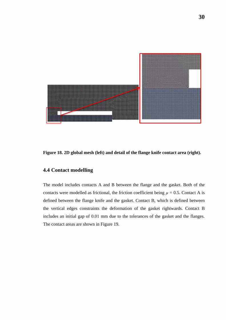
4.3 Mesh
The flange and the gasket were meshed with 2D quadrilateral elements with mid-side
nodes activated. The average value of the mesh size is 0.02 mm, resulting in 44 787
elements and 135 893 nodes. Global mesh of the flange assembly and a detail of the
flange knife area are presented in Figure 18.
30
Figure 18. 2D global mesh (left) and detail of the flange knife contact area (right).
4.4 Contact modelling
The model includes contacts A and B between the flange and the gasket. Both of the
contacts were modelled as frictional, the friction coefficient being µ = 0.5. Contact A is
defined between the flange knife and the gasket. Contact B, which is defined between
the vertical edges constraints the deformation of the gasket rightwards. Contact B
includes an initial gap of 0.01 mm due to the tolerances of the gasket and the flanges.
The contact areas are shown in Figure 19.

31
Figure 19. Contact definitions for 2D analysis.
4.5 Boundary conditions
Three boundary conditions, shown in Figure 20, were applied to the model. Boundary
condition C is an imposed displacement up to the symmetry line. Because only half
(one flange and half of the gasket) of the geometry was modelled, boundary condition D
was added to represent the symmetry, while boundary condition E constraints the left
side of the flange.
C: y = imposed displacement to the symmetry line
D: y = 0 (symmetry)
E: x = 0

32
Figure 20. Boundary conditions for 2D analysis.

33
5 3D FINITE ELEMENT MODEL DESCRIPTION
This chapter describes in detail the 3D finite element model.
5.1 Model
3D model was created in ANSYS Workbench FEA software to evaluate the
deformations of the gasket for versions 1, 7 and 12. In particular, on the basis of 2D
results, version 7 had the minimum deformations, while version 12 had the maximum
deformations. Because of symmetry only 1/8 of the geometry was used. In Figure 21, L
refers to the long face of the gasket, while S refers to the short face of it. As in 2D
simulation, large deformation option was enabled to take into account large strains
occurring in the gasket.
Figure 21. Left: Assembly of the flanges and the gasket (half). Right: A view of the
finite element geometry (L: long face of the gasket, S: short face of the gasket).

34
5.2 Material
The same material models as in the 2D simulation (chapter 4.2) were used.
5.3 Mesh
The gasket was meshed with hexagonal cube elements and the flange with tetrahedrons,
mid-side nodes being activated in both parts; in order to improve the accuracy of the
simulation and to reduce the computational time, the mesh was refined in the contact
area. The average value of the mesh size is 0.1 mm, resulting in 189 378 elements and
478 009 nodes (Figure 22).
Figure 22. Left: Global mesh. Right: Detailed view of the contact area.
5.4 Contact modelling
Three contacts were defined for the analysis (Figure 23). Contacts A and B are defined
between the vertical surfaces of the flange and the external surfaces of the gasket, so
that the outward expansion of the gasket is constrained by the internal surfaces of the
flange. Contact C, defined between the flange knife and the gasket, is transferring the
load from the flange to the gasket. Friction coefficient µ = 0.5 was used for all the
contacts.

35
Figure 23. Contact definition for the 3D modelling.
5.5 Boundary conditions
Boundary conditions are presented in Figure 24. The symmetry boundary D condition
was reproduced using frictionless supports. Displacement boundary condition E was
applied to the bottom surface of the flange.

36
Figure 24. Symmetry boundary condition (D) and displacement boundary
condition (E).

37
6 RESULTS
In this chapter the results of the finite element simulations using both 2D and 3D
elements are presented and compared.
6.1.1 2D plane stress and strain modelling
Twelve versions of different flange knife dimensions were simulated.
Figure 25 shows deformations in the x direction for flange version 1 using plane strain
elements. The elements near the flange knife were the most distorted during the
simulation, thus leading to convergence problems, especially for versions having the
highest final deformations. Table 4 presents the maximum deformation values of the
gasket in the x direction for all the case studies, the maximum being at point A. From
the results it can be observed that as the width and the length of the knife increase, the
gasket deforms more. Version 12, having the largest flange knife dimensions, yields the
maximum deformations (maximum 234 µm) of the gasket.

38
Figure 25. Top: Deformations in the x direction. Bottom: Detailed view of
deformations in the flange knife area (version 1).
Table 4. Maximum deformation of the gasket in 2D plane strain model.
Version a (mm) b (mm) Plane strain: directional deformation at
point A (µm)
1 0.75 0.35 -122 2 0.75 0.3 -171 3 0.5 0.35 -101 4 0.5 0.3 -139 5 1 0.35 -140 6 1 0.3 -187 7 0.5 0.4 -59 8 0.5 0.25 -179 9 0.75 0.4 -78
10 0.75 0.25 -212 11 1 0.4 -89 12 1 0.25 -234
39
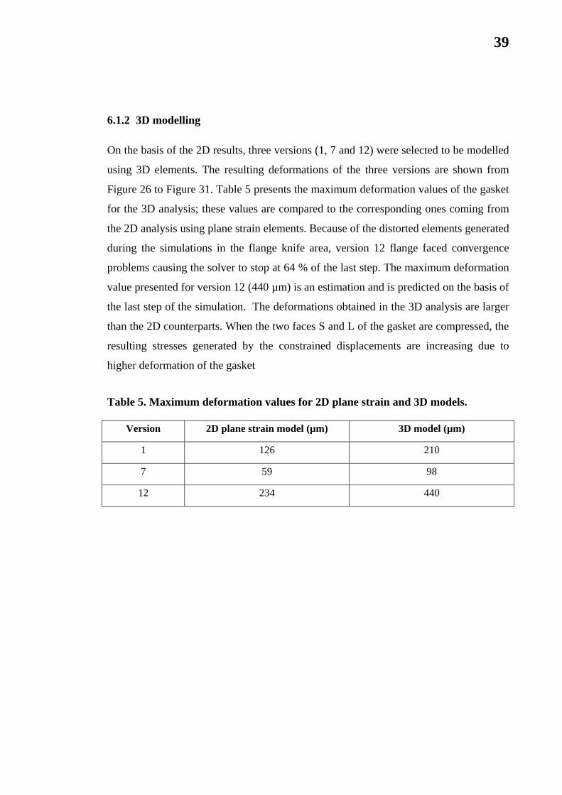
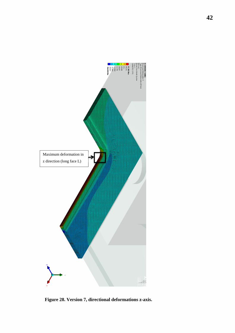
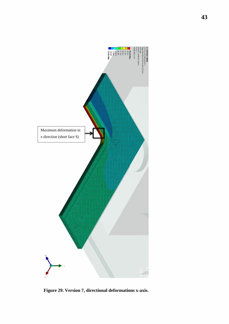
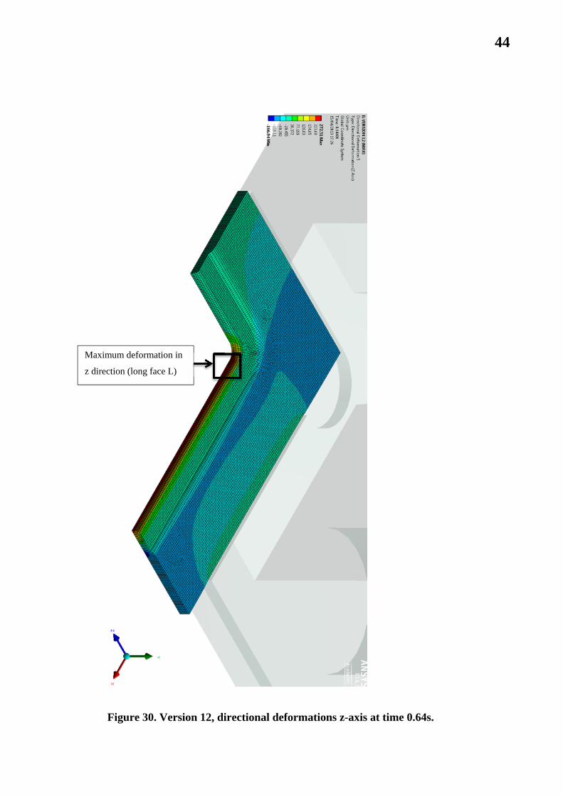
6.1.2 3D modelling
On the basis of the 2D results, three versions (1, 7 and 12) were selected to be modelled
using 3D elements. The resulting deformations of the three versions are shown from
Figure 26 to Figure 31. Table 5 presents the maximum deformation values of the gasket
for the 3D analysis; these values are compared to the corresponding ones coming from
the 2D analysis using plane strain elements. Because of the distorted elements generated
during the simulations in the flange knife area, version 12 flange faced convergence
problems causing the solver to stop at 64 % of the last step. The maximum deformation
value presented for version 12 (440 µm) is an estimation and is predicted on the basis of
the last step of the simulation. The deformations obtained in the 3D analysis are larger
than the 2D counterparts. When the two faces S and L of the gasket are compressed, the
resulting stresses generated by the constrained displacements are increasing due to
higher deformation of the gasket
Table 5. Maximum deformation values for 2D plane strain and 3D models.
Version 2D plane strain model (µm) 3D model (µm)
1 126 210
7 59 98
12 234 440

40
Figure 26. Version 1, directional deformations z-axis.
Maximum deformation in
z direction (long face L)
41
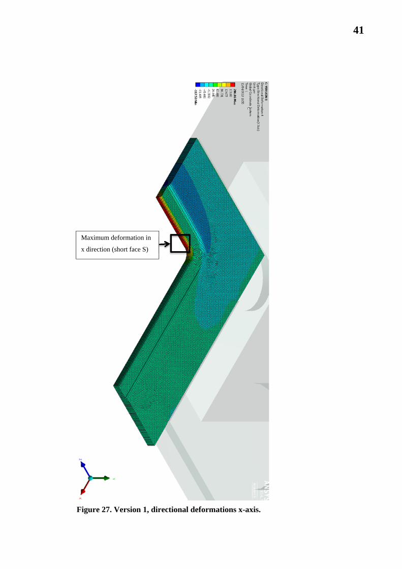
Figure 27. Version 1, directional deformations x-axis.
Maximum deformation in
x direction (short face S)
42
Figure 28. Version 7, directional deformations z-axis.
Maximum deformation in
z direction (long face L)
43
Figure 29. Version 7, directional deformations x-axis.
Maximum deformation in
x direction (short face S)
44
Figure 30. Version 12, directional deformations z-axis at time 0.64s.
Maximum deformation in
z direction (long face L)

45
Figure 31. Version 12, directional deformations x-axis at time 0.64s.
Maximum deformation
in x direction (short
face S)

46
7 CONCLUSIONS AND FUTURE STEPS
The newly designed x-band RF flange assembly was simulated with ANSYS FEA
software. Twelve different versions of flanges were simulated using 2D plane stress and
plane strain elements. Three of these versions were also modelled using 3D elements.
The resulting deformations obtained using plane stress elements were smaller than the
ones obtained with plane strain elements; in particular in the first case, deformations
perpendicular to the plane were allowed and no additional stresses were contributing to
the total deformation of the gasket. By comparing these results with the ones obtained
using solid elements, it can be seen that the deformations in the 3D analysis are even
bigger, since the lateral faces of the flange taken into account in this modelling are
constraining further the expansion of the gasket in the other directions, thus resulting in
additional stresses. Overall, the deformations obtained for all the versions are meeting
the specified requirements.
In the next future, experimental tests will be conducted at CERN and the theoretical
results presented in this thesis will be validated.
47
8 REFERENCES
Stapnes et al. (2012) A Multi-TeV linear collider based on CLIC technology: CLIC
Conceptual Design Report. CERN 2012-007.
Askeland et al. (2010) Essentials of Materials Science and Engineering. Stamford:
Cengage Learning.
Beer et al. (2012) Mechanics of Materials. New York: McGraw-Hill.
Callister WD Jr (2001) Fundamentals of Materials Science and Engineering. New York:
John Wiley & Sons.
CERN (2013) About CERN. http://home.web.cern.ch/about. [1.4.2013]
CERN (2013) Member states. http://home.web.cern.ch/about/member-states. [1.4.2013]
CERN (2010) Physics for health. http://physics-for-health.web.cern.ch/physics-for-
health. [1.4.2013]
Ellis JR (2000) Physics Goals of the Next Century at CERN. CERN-TH-2000-050.
Ellis JR & Wilson I (2000) New Physics with the Compact Linear Collider. CLIC-Note-
466.
Geschonke G (2010) The Next Energy-Frontier Accelerator a Linear e+e- Collider?.
CERN-OPEN-2010-007. CLIC-Note-807.
Martin J (2006) Materials for engineering. Cambridge: Woodhead Publishing Limited
and Maney Publishing Limited.

48
Roylance D (2000) Introduction to Elasticity. Cambridge: Department of Materials
Science and Engineering.
Smallman RE (1999) Modern Physical Metallurgy & Materials Engineering. Oxford: A
division of Reed Educational and Professional Publishing Ltd.
ANSYS Workbench ™, ANSYS, Inc.
MatWeb. Material property data.
http://www.matweb.com/Search/MaterialGroupSearch.aspx?GroupID=179
[1.4.2013]

49
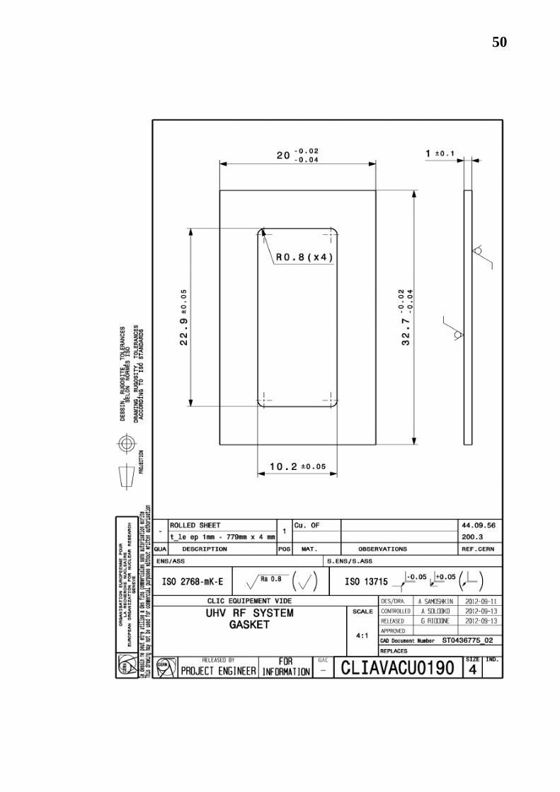
APPENDIX 1 DETAILED DRAWINGS OF THE FLANGE AND THE GASKET
50
Recommended