Financing Local Development: Quasi-Experimental Evidence fromMunicipalities in Brazil, 1980-1991�
Stephan Litschig�
June 22, 2012
Abstract
This paper uses a regression discontinuity design to estimate the impact of additional unre-
stricted grant �nancing on local public spending, public service provision, schooling, literacy, and
income at the community (município) level in Brazil. Additional transfers increased local pub-
lic spending per capita by about 20% with no evidence of crowding out own revenue or other
revenue sources. The additional local spending increased schooling per capita by about 7% and
literacy rates by about 4 percentage points. The implied marginal cost of schooling�accounting
for corruption and other leakages�amounts to about US$ 126, which turns out to be similar to
the average cost of schooling in Brazil in the early 1980s. In line with the effect on human capital,
the poverty rate was reduced by about 4 percentage points, while income per capita gains were
positive but not statistically signi�cant. Results also suggest that additional public spending had
stronger effects on schooling and literacy in less developed parts of Brazil, while poverty reduction
was evenly spread across the country.
Keywords: intergovernmental grants, decentralization, economic developmentJEL: D70, H40, H72, O15
�Discussion and results in this paper's sections 2.1, 2.2, 3.2, 4, 5, 6, 7.1, tables 2, 3, 5 and �gures 1, 2, 3, and 4 areidentical or essentially identical to corresponding sections, tables, and �gures in Litschig and Morrison (2012). This paperrevises and extends a version from 2008, which was entitled "Intergovernmental Transfers and Elementary Education:Quasi-Experimental Evidence from Brazil". I am grateful to Antonio Ciccone, Rajeev Dehejia, Claudio Ferraz, AlbertFishlow, Patricia Funk, José Garcia Montalvo, Wojciech Kopczuk, David Lee, Leigh Linden, Bentley MacLeod, KevinMorrison, Gaia Narciso, Kevin O'Rourke, Steve Pischke, Kiki Pop-Eleches, Bernard Salanié, Joseph Stiglitz, AlessandroTarozzi, Miguel Urquiola, Pedro Vicente and Till von Wachter for their comments and support throughout this project. Ialso received helpful feedback from seminar participants at the Center for Global Development, Columbia University, FGVRio de Janeiro, the Harris School, UC Merced, University of Montreal, Universitat Pompeu Fabra, University of Toronto,Trinity College Dublin, the BWPI summer school 2007 at Manchester University, and the 2007 NSEA conference in St.Gallen. I thankfully acknowledge �nancial support from David Lee and the Department of Economics, PER and ILAS atColumbia University. All remaining errors are my own.�Universitat Pompeu Fabra and Barcelona GSE, [email protected].
1

1 Introduction
Many economists are skeptical whether making more funds available to governments in poor coun-
tries leads to better development outcomes (Easterly 2006, 2008). Similar skepticism applies to
intergovernmental transfers, and more speci�cally to whether providing additional �nancing to
local governments in developing countries raises living standards of the local population (Shah
2006).1 The reasons to worry are many, including corruption (Reinikka and Svensson 2004; Olken
2007; Ferraz and Finan 2008), simple waste in the provision of public services (Bandiera, Prat,
and Valletti 2009), and capture of the political process by the local elite (Bardhan and Mookherjee
2005). Moreover, funds might be rationally crowded out by benevolent and ef�cient local gov-
ernments and even the money that ends up being spent on actual service improvements might fail
to have the intended impact. Given these facts and concerns about local government spending,
it is not clear ex ante to what extent providing more �nancing improves public service delivery
at the margin. However, due to high data requirements, there is very little research that looks at
the impact of additional �scal transfers on public services and development outcomes, such as
human capital accumulation and earnings. Since intergovernmental transfers �nance a large share
of decentralized public service provision in developing countries around the world (Rodden 2004,
Shah 2006), it is important to know to what extent additional funding to local governments actually
"trickles down" to the population.
This paper provides the �rst quasi-experimental evidence regarding the impact of intergovern-
mental transfers on local public services and living standards in a developing country. I analyze
the effect of additional unrestricted grant �nancing on local public spending, public service provi-
sion, schooling, literacy, and income at the community (município) level in Brazil over the period
1980-1991.2 Municipalities in Brazil elect their own local executives and legislators who are in
charge of local spending, mainly on education, housing and urban infrastructure, and transporta-
tion. Brazil does not have a good reputation in terms of public governance in general3 and there
is recent objective evidence of corruption in the local delivery of centrally funded services from1Shah starts his review of the literature with the following (anonymous) quote: "The practice of intergovernmental �scal
transfers is the magical art of passing money from one government to another and seeing it vanish in thin air."2Municipalities are the lowest level of government in Brazil (below the federal and state governments). The discussion
refers to counties, communities or municipalities interchangeably.3According to Transparency International's Corruption Perception Index for 1995 (the earliest available year), Brazil
ranked as the �fth most corrupt out of 41 surveyed countries.
2

audit reports (Ferraz and Finan 2008). Moreover because about 40% of the Brazilian population
was illiterate and therefore did not have the right to vote until 1985, concerns about elite capture
of the local political process are likely to apply.
In order to address the likely endogeneity of central government funding, my identi�cation
strategy exploits the fact that a substantial part of national tax revenue in Brazil is redistributed
strictly on the basis of population, via a formula based on cutoffs. That is, if a municipality's
population is over the �rst population cutoff, it receives additional resources, over the second
threshold a higher amount, and so forth. Around the population cutoffs there are thus jumps in
per capita central government funding and local public spending which are "as good as" randomly
assigned (under relatively weak, and to some extent testable, assumptions further discussed below).
The main empirical result of the paper is that communities that received extra �nancing from the
central government over the period 1982-1985 bene�ted in terms of education outcomes (higher
schooling4 and literacy rates) and income (lower poverty rates), measured in 1991.5 Some of the
channels through which these effects on living standards arose were as follows: Additional trans-
fers increased local public spending per capita by about 20%, with no evidence of crowding out
own revenue or other revenue sources. Local spending shares remained essentially unchanged, that
is, local spending on education, housing and urban infrastructure, and transportation all increased
by about 20% per capita. Direct evidence on public service improvements is mixed: while there
is some indication that student-teacher ratios in local primary school systems fell, there is little
evidence that housing and urban development spending affected housing conditions.
An important limitation of looking at direct public service measures is that there are no data on
what the money was actually spent on, and so it is dif�cult to know whether the available measures
are the "right" ones. Quality improvements and repairs, for example, would be impossible to detect
with simple quantity measures of public services. In order to deal with this issue, I also investigate
whether the extra spending affected household income and municipal education outcomes, as mea-
sured by community average schooling and literacy rates. Education outcomes and earnings can4Schooling refers to completed grades, not "years in school".5I focus on the beginning of the 1980s because starting in 1988, of�cial population estimates were updated annually,
which meant that the magnitude of the variation in funding at the cutoffs was signi�cantly reduced (Supplementary Law no59/1988). In addition, there is strong evidence of manipulation of the 1991 estimates, which determined transfers throughthe entire decade of the 1990s and beyond (Litschig 2008).
3

be thought of as indirect summary measures of public services: extra public spending on education
should improve the quality of local schools, thus increasing the marginal bene�t of education for
any given level of schooling (Behrman and Birdsall 1983). At the same time, other public inputs,
such as spending on road quality, should reduce the marginal cost of schooling, thus increasing
households' equilibrium schooling choice (Birdsall 1985; Behrman, Birdsall, and Kaplan 1996).
The results for education outcomes suggest that the relevant school-age cohorts acquired about
0.3 additional years of schooling per capita (a 7% increase), and literacy rates increased by about
four percentage points on average (compared to a 76% literacy rate in the comparison commu-
nities). In order to interpret these results, it is useful to consider the marginal cost of a year of
schooling implied by these estimates and compare it to the average cost of schooling in Brazil
at the time. This requires some assumptions, but a rough comparison can be made. My back-
of-the-envelope calculations suggest that the implied marginal cost of schooling�accounting for
corruption and other leakages�amounts to about US$ 126, which turns out to be similar to the
average cost of schooling in Brazil in the early 1980s. While these are rough estimates, the simi-
larity of the marginal cost to the average cost indicate that the �ndings here are certainly plausible.
Moreover these estimates suggest that�accounting for corruption and other leakages�providing
more �nancing to local governments at the margin improved education outcomes at reasonable
cost.
In turn, better and more widespread education and better local public service quality overall
(better infrastructure and primary health care for example) are likely to increase household in-
comes. The evidence suggests that the extra public spending indeed had an effect on income,
although only for the poor. Speci�cally, I �nd that the poverty rate (measured relative to the na-
tional income poverty line) was reduced by about 4 percentage points from a comparison group
mean poverty rate of 64%. Income per capita gains were positive but not statistically signi�cant.
The income gains for the poor are unlikely to be driven by direct welfare transfers since these were
negligible at the time, and also since income was measured in 1991 and the funding differential
lasted only until the end of 1985. My back-of-the-envelope calculations suggest that about 2 per-
centage points of the poverty reduction are plausibly accounted for by the education channel alone,
leaving the remaining 2 percentage points to better local public service quality overall.
4

Brazil is a very diverse country and so it is instructive to evaluate whether the impacts of local
public spending on schooling and income vary depending on existing levels of development in
1980. Assuming a decreasing marginal productivity of local spending, one would expect stronger
effects in the less developed northern parts of the country, all else equal.6 All else might not be
equal, however. In particular, governance might be generally worse in the North and thus extra
resources received might not be spent as productively as in the South. Moreover, asymmetries
in political awareness and participation of the poor might be higher in the less developed North,
leading to a public service provision that is less responsive to the needs of the poor (Bardhan and
Mookherjee 2005). Results suggest that the same additional public spending had stronger effects
on schooling and literacy in the North of Brazil, while the effect on poverty reduction was evenly
spread across the country. In addition, I also �nd stronger effects on schooling in more rural
compared to more urban municipalities, which would be consistent with the larger role municipal
governments play in the provision of elementary education in rural areas.
In order to assess the internal validity of these results, I run a series of tests and robustness
checks. First, there is no evidence of manipulation of the 1980 census municipality population
�gures. Second, I verify whether municipalities in the marginal (to the cutoff) treatment and com-
parison groups were ex ante comparable7 by testing for discontinuities in pre-treatment covariates
such as whether the municipality was aligned with the central government in 1982, municipality
own and total revenues, income per capita, poverty, urbanization, elementary school enrollment,
schooling, literacy, and infant mortality. The results show that there is no statistical evidence of
discontinuities in these potentially confounding factors although some of the point estimates sug-
gest that treatment group municipalities were already doing somewhat better than those in the
comparison group as of 1980. Third, I show that all results are robust to both the inclusion of
pre-treatment covariates (including pre-treatment education and earnings outcomes) and to the
choice of bandwidth and functional form. Fourth, I show that the education gains are robust to a
difference-in-differences approach that directly controls for pre-treatment schooling differences of
elementary-school-age cohorts. In contrast, the corresponding difference-in-differences estimates6Local inputs might also be cheaper in less developed parts of the country.7Municipalities in the marginal treatment (comparison) group are those whose 1980 census population falls in the interval
c; cC " .c� "; c/, where c is a cutoff and " some small number relative to municipality population.
5

for cohorts that have largely completed their education�and for whom one would expect smaller
or no impacts�are close to zero in magnitude and very far from statistical signi�cance.8 Finally, I
�nd almost identical results when I restrict the sample to individuals who were born in the munici-
pality and never moved away, which suggests that the schooling and literacy gains were not driven
by selective migration.
It is worth emphasizing that the estimates reported here represent effects of local public spend-
ing increases for the subpopulation of municipalities with populations at or near the cutoffs spec-
i�ed in the revenue-sharing mechanism.9 Because I �nd similar effects at these cutoffs, however,
results are likely to generalize to small local communities in Brazil. Whether providing additional
�nancing to local governments in other contexts would yield similar results is an open empirical
question. The most closely related study investigates the effects of oil windfalls on local spending
and living standards also at the local level in Brazil, albeit in a later period and using a different
design (Caselli and Michaels 2009). Their results suggest that additional local public spending
�nanced through royalties had little if any effect on local public services or household income per
capita, although in some speci�cations they also �nd a reduction in the poverty rate.
Existing studies on the effects of unconditional grants have tended to focus on spending deci-
sions by the local community without evaluating effects on public services or human capital and
earnings outcomes. Speci�cally, the result obtained here that additional transfers to local govern-
ments increased local public spending one-for-one, with no evidence of crowding out own revenue
or other revenue sources, has been found in many previous studies in the literature on intergov-
ernmental grants and local spending.10 This empirical regularity is referred to as the "�ypaper
effect", since the grant money sticks where it hits (the public budget) rather than �nding its way
into private budgets (through tax breaks or direct transfers), which is what theory would predict if
transfer income and private income were perfectly fungible and local government spending deci-8Strictly speaking this is not a placebo experiment. Although one would expect smaller effects on education outcomes
for cohorts that were beyond regular elementary schooling age, the effect need not be zero since older cohorts mighthave attended adult literacy programs that were promoted by the military government, such as the MOBRAL (MovimentoBrasileiro de Alfabetização), and offered through the local administration.9See Lee (2008) for an alternative interpretation of the treatment effect identi�ed in an RD analysis as a weighted average
of individual treatment effects where the weights re�ect the ex ante probability that an individual´s score is realized closeto the cutoff.10The result is less surprising for the relatively small local governments considered in this study, since they collect onlyabout 6% of total revenue from their own residents and therefore have only little room to give tax reductions. I cannotsay whether such low own-revenue collection represents an optimal choice or whether it re�ects an inability to raise morerevenue locally. See Hines and Thaler (1996) for a review of the �ypaper literature and problems with the empirical work.
6

sions re�ected preferences of voters (Bradford and Oates 1971).
While the effects on education and income presented here are best interpreted as local public
spending or public service quality effects, it is useful to contrast these �ndings with those of the
aggregate (state, district, or community) literature on school quality or school resource effects.
In fact, the distinction between this study and most existing aggregate studies on school quality,
education, and earnings might not be very signi�cant in practice, since these aggregate studies
typically use measures of school resources that are likely correlated with other dimensions of the
public service environment.11
The positive effects on educational attainment (completed years of schooling) reported here
are qualitatively consistent with aggregate studies in the U.S. and in developing countries.12 The
positive effects on educational achievement (literacy) are also in line with most of the estimates
in the aggregate literature that evaluates effects on test scores, which is summarized by Hanushek
(2006).13 However, in contrast to most of these studies, the results presented here are comfortably
signi�cant at conventional levels. The poverty reduction estimated here is also in line with most
of the aggregate literature for the US, which tends to �nd positive and statistically signi�cant
effects on earnings (Card and Krueger 1996). For developing countries, the aggregate evidence
on school quality and earnings is scant, except for Du�o's (2001) study on school construction in
Indonesia, which shows positive effects on earnings (in addition to positive effects on schooling),
and Behrman and Birdsall (1983) and Behrman, Birdsall and Kaplan (1996), who also estimate
positive returns to school quality in Brazil.
Needless to say, the results that transfers were spent one-for-one and that they had an impact on
education and earnings outcomes do not imply that none of the extra funds were privately appropri-
ated by the incumbent, wasted or used for political patronage. Indeed, some of the reported extra
spending likely never translated into service improvements "on the ground" for precisely these rea-11Behrman and Birdsall (1983) and Birdsall (1985) use average schooling of teachers and average teacher income acrossgeographical areas in Brazil. Card and Krueger (1992) use teacher-student ratios, average teacher pay, and length of theschool year across states in the U.S.12For aggregate evidence for the U.S. see Card and Krueger (1992) and Heckman, Layne-Farrar, Todd (1996). Fordeveloping countries see Birdsall (1985) for Brazil, Lavy (1996) for Ghana, Case and Deaton (1999) for South Africa andDu�o (2001) for Indonesia. For micro studies see Chin (2005) and Banerjee, Jacob, Kremer, Lanjouw and Lanjouw (2000)for evidence on India. Glewwe, Kremer and Moulin (2009) provide evidence for Africa.13See Hoxby (2000) and Hanushek (2006) for a skeptical reading of the evidence on resource effects in education, bothin the US and in developing countries. See Krueger (2003) and Krueger and Whitmore (2001) for the view that additionaleducation resources, class size reductions in particular, do matter in the US.
7

sons and there is recent direct evidence to back this up. Speci�cally, Brollo, Nannicini, Perotti and
Tabellini (2010) adopt the identi�cation strategy of this paper and use the audit reports in Ferraz
and Finan (2008), to show that municipalities that got a windfall of the same unrestricted funds an-
alyzed here also experienced a roughly proportional increase in public management irregularities.
They also provide evidence that the quality of candidates running for local of�ce deteriorated in
these municipalities. Increasing the accountability of both local politicians and service providers is
therefore likely to improve public service quality, as discussed in Bjoerkman and Svensson (2009)
for example. The results presented here do suggest, however, that even in the absence of reforms
that strengthen local accountability, and despite well founded worries about corruption, other leak-
ages, and local capture, local governments in Brazil did use the additional funds they received to
expand public services to the general local population at reasonable cost.
The remainder of the paper is organized as follows: Section 2 documents the role of local
governments in public service provision in Brazil and gives institutional background on revenue
sharing. Section 3 provides the conceptual framework and discusses the identifying assumptions
for a causal interpretation of the estimates presented in this paper. Section 4 describes the data.
Section 5 discusses the estimation approach and Section 6 evaluates the internal validity of the
study. Section 7 presents the main results. Section 8 provides further robustness checks. Section 9
discusses heterogeneity of impacts depending on the initial level of development of the municipal-
ity. The paper concludes with a discussion of limitations and extensions.
2 Background
2.1 Local public services and their �nancing in Brazil
Local government responsibilities at the beginning of the 1980s were mostly to provide elemen-
tary education, housing and urban infrastructure as well as local transportation services.14 Because
municipalities have never collected much in the way of own revenues, intergovernmental transfers
were essential to their functioning. In the early 1980s, total government revenue in Brazil was
about 25% of GDP, of which municipalities collected about 4%. At the same time, local govern-14Local governments also provided some primary health care services (about 10% of local budgets). Local welfareassistance was close to negligible at the beginning of the 1980s.
8

ments managed about 17% of public resources (Shah 1991). In other words, intergovernmental
transfers to local governments represented about 3.25% of GDP. The most important among these
transfers was the federal Fundo de Participação dosMunicípios (FPM), a largely unconditional rev-
enue sharing grant funded by federal income and industrial products taxes.15 This grant accounted
for about 50% of the revenue of the municipalities used in this study.
In the empirical analysis below, I estimate the effect of additional FPM �nancing over the
four year period 1982-1985 on local public spending, public service provision, schooling, literacy,
and income. The public service indicators I consider are dictated by data availability. They are
measured in 1991, the earliest post-treatment year for which comprehensive data on municipalities
are available. The indicators are supposed to capture improvements in the main spending areas of
education as well as housing and urban infrastructure. Unfortunately I do not have any indicators
on local transportation services or infrastructure.
In the area of education, I use the teacher-student ratio in municipal elementary schools and
the number of schools run by the municipal government. It is easy to see how extra spending
over the period 1982-1985 might affect the number of schools six years later in 1991. Effects on
teacher-student ratios in 1991 might arise if the extra spending on education was in fact smoothed
over subsequent years or if additional teachers could not easily be dismissed once the funding
differential stopped. Public service measures in the area of housing and urban infrastructure are
the percentages of individuals in the municipality with access to water, sewer, electricity and living
in substandard housing.
I also use education outcomes for the relevant school-age population, measured in 1991, as
indirect summary measures of public service improvements. Public provision of elementary edu-
cation in Brazil was for the most part a joint responsibility of state and local governments, while
the federal government was primarily involved in �nancing and standard setting. Of total public
elementary education spending in the early 1980's, local governments accounted for about 26%,
while state governments accounted for about 65%, with the remainder accounted for by the federal
government. About 21% of local government budgets were devoted to education, with the bulk15 The one condition is that municipalities must spend 25 percent of the transfers on education. This constraint is usuallyconsidered non-binding, in that municipalities typically spend about 20% of their total revenue on education. It is not clearhow this provision was enforced in practice since there is no clear de�nition of education expenditures and accountinginformation provided by local governments was not systematically veri�ed.
9

(72%) going to fundamental education (grades 1-8) and the remainder to intermediary education
(grades 9-12) (World Bank 1985).
In 1980, 55% of all elementary school students in Brazil were enrolled in state administered
schools, 31% in municipality schools and the remaining 14% in private schools. In small and rural
municipalities, such as those considered here, the proportion of students in schools managed by
local governments was 0.74 while the proportions for state-run and private schools were 0.24 and
0.02, respectively. Elementary school was compulsory for 7-to 14-year-olds, but less than 14% of
an age cohort in 1980 completed the 8 grades of compulsory schooling in 8 years. The average
number of completed grades after 8 years in school was about 5. Individuals were eligible to
attend regular elementary school until the age of 18 and regular secondary school until the age of
21. Beyond these age limits individuals had to enroll in special education classes (World Bank
1985).
2.2 Mechanics of revenue sharing in Brazil
In order to estimate the effect of additional grants on local living standards, I exploit variation
in FPM funding at several population cutoffs using regression-discontinuity (RD) analysis. The
critical feature of the FPM revenue-sharing mechanism for the purposes of this analysis is Decree
1881/81, which stipulates that transfer amounts depend on municipality population in a discontin-
uous fashion. More speci�cally, based on municipality population estimates, pope, municipalities
are assigned a coef�cient k D k.pope/, where k(.) is the step function shown in Table 1. For
counties with up to 10'188 inhabitants, the coef�cient is 0.6; from 10'189 to 13'584 inhabitants,
the coef�cient is 0.8; and so forth. The coef�cient k.pope/ determines the share of total FPM
resources, revt , distributed to municipality m in year t according to the following formula:
FPMmt Dk.popem/Pmkm
revt
This equation makes it clear that local population estimates should be the only determinant of
cross-municipality variation in FPM funding. Exact county population estimates are only available
for census years or years when a national population count is conducted. Transfers were allocated
based on 1980 census population from 1982 (the �rst year the 1980 census �gures were used)
10

until 1985.16 Previously, from 1976 to 1981, the transfers had been based on extrapolations from
the 1960 and 1970 censuses, produced by the national statistical agency, IBGE.17 Likewise, from
1986 to 1988, the transfers were also based on such extrapolations, this time based on 1970 and
1980 census population �gures.18 As a result of the update in 1986, the funding discontinuities
for those municipalities around the cutoffs based on the 1980 census disappeared because many
municipalities changed brackets due to decreases or, more often, increases in their population
relative to 1980.19 The "treatment" therefore consists of a (presumably) unexpected temporary
funding windfall to the municipal budget, which lasted for four years from the beginning of 1982
through the end of 1985.
While this design of the revenue sharing mechanism is fortunate for scienti�c purposes, it also
represents somewhat of a puzzle: why would politicians allocate resources based on objective cri-
teria, such as population, rather than use discretion? The answer to this question lies in the political
agenda of the military dictatorship that came to power in 1964. As detailed by Hagopian (1996),
one of the major objectives of the military was to wrest control over resources from the traditional
political elite and at the same time to depoliticize public service provision. The creation of a rev-
enue sharing fund for the municípios based on an objective criterion of need, population, was part
of this greater agenda. It re�ected an attempt to break with the clientelistic practice of the tradi-
tional elite, which manipulated public resources to the bene�t of narrowly de�ned constituencies.
The reason for allocating resources by brackets, i.e. as a step function of population as in Decree
1881/81, is less clear. One explanation could be that compared to a linear schedule, for example,
the bracket design mutes incentives for local of�cials at the interior of the bracket to tinker with
their population �gures or to contest the accuracy of the estimates in order to get more transfers. A
related question is where the exact cutoffs come from�that is, why 10'188, 13'584, 16'980, and
so forth? While I was unable to trace the origin of these cutoffs precisely, I know roughly how they
came about. The initial legislation from 1967 created cutoffs at multiples of 2'000 up to 10'000,16The 1985 of�cial estimates were already based on extrapolations which resulted in minor changes compared to the 1980census numbers.17The methodology used by the statistical agency in principle ensures that population estimates are consistent betweenmunicipalities, states, and the updated population estimate for the country as a whole (Instituto Brasileiro de Geogra�a eEstatística 2002).18Beginning in 1989 the population estimates were updated on a yearly basis.19To be clear, there are no economically or statistically signi�cant differences in FPM transfers between the treatment andcomparison group (those around the �rst three cutoffs based on the 1980 census) from 1986 onwards. Results are omittedto save space and are available upon request.
11

then every 4'000 up to 30'000 and so forth. The legislation also stipulated that these cutoffs should
be updated proportionally with population growth in Brazil.20 The cutoffs were thus presumably
updated twice, once with the census of 1970 and then with the census of 1980, which explains
the "odd" numbers. It is noteworthy that the thresholds are still equidistant from one another, the
distance being 6'792 for the �rst seven cutoffs (except for the second cutoff, which lies exactly
halfway in between the �rst and the third cutoffs).
Perhaps most important for this analysis is that over the study period, the transfers were in
fact allocated as stipulated in Decree 1881/81. Figure 1 plots cumulative FPM transfers over the
period 1982 to 1985 against 1982 of�cial population. Each dot in this �gure corresponds to a
municipality. The horizontal lines correspond to the modal levels of cumulative transfers for each
bracket in the data. The �gure shows that funding jumps by about 1'320'000 Reais (2008 prices) or
about 1'000'000 international US$ at each threshold over this period.21 Observations that appear
above or below the horizontal lines are most likely due to measurement error, because transfer data
in this �gure are self-reported by municipalities, rather than based on administrative records of the
Ministry of Finance, which are not available for the period considered.22 The cumulative transfer
differential over the period 1982-1985 corresponds to about 2.5% of annual GDP in rural areas of
the country and about 1.4% of annual GDP in urban areas for the counties in the estimation sample
(Table 2).
Although the funding jump is the same in absolute terms at each cutoff, the jump declines in
per capita terms the higher the cutoff. As is apparent from Figure 1, funding jumps by about R$
130 (US$ 95) per capita at the �rst threshold, R$ 97 (US$ 70) at the second, R$ 78 (US$ 57) at the
third, and declines monotonically for the following cutoffs (R$ 55, R$ 43 and R$ 35, respectively).
Immediately to the left of the �rst three cutoffs, per capita FPM funding is about R$ 390 (286
US$), and this amount declines monotonically for the following cutoffs. For the �rst three cutoffs
the funding increase per capita is therefore from the same baseline level and represents about 33%
at the �rst, 25% at the second, and 20% at the third cutoff. Though the differences are not great,
this means that the treatment in terms of additional per capita funding is not exactly the same20Supplementary Law No. 35, 1967, Art. 1, Paragraphs 2 and 4.21The 2005 Real/$ PPP exchange rate was about 1.36 (World Bank 2008).22For later periods the data is available from the Ministry of Finance, and in these data there is essentially no variation inFPM transfers for a given state and population bracket.
12

across these cutoffs. However, since there are likely to be economies of scale in the provision of
local public services�that is, unit costs decline with scale�the differences in treatment across
cutoffs might be even smaller than what the per capita funding jumps would suggest. It thus seems
reasonable to expect similar treatment effects around these cutoffs, as further discussed in Section
5 below.
3 Conceptual framework and identi�cation
3.1 Conceptual framework
Because the additional FPM transfers provide unrestricted budget support, effects on schooling
and income may arise through a variety of channels in addition to education spending, such as
improved local roads, for example. The following presents a framework for thinking about the
causal effects estimated here and compares them to the micro and aggregate literatures on school
resources, schooling, and earnings.
Assume that schooling S in the local community depends on public spending on education E ,
for example through class size C; and on another public input, say transportation infrastructure T;
which in turn both depend on the overall level of local public spending or resources R of which
FPM transfers F represent an important share. Also assume that household income I depends
on schooling and local public service quality (transportation infrastructure for example). These
relations can be summarized as follows:
S D S.C.E.R.F///; T .R.F///
I D I .S.:/; T .R.F///
Micro studies would typically estimate the effect of providing real resources to particular
schools or classrooms, i.e. they would evaluate the partial derivatives SC or IC for example. In
contrast, the effects estimated here can be thought of as SF and IF which represent total deriva-
tives of schooling and income with respect to �nancial resource transfers, i.e. they capture effects
arising through multiple spending channels, not just education spending. In particular, SF and IF
both incorporate RF , the marginal propensity to spend transfers received and ER and TR , the mar-
13
ginal propensities to spend on education and transportation infrastructure, respectively. These total
derivatives may be higher or lower than those from speci�c education or infrastructure projects,
depending on complementarities between these interventions.
The contribution of this paper is to provide the �rst quasi-experimental estimates of SF and IF ,
the effects of �nancial transfers on schooling and income, respectively. Existing aggregate studies
on resource effectiveness in the education sector essentially evaluate SE and IE . The distinction
between this study and most existing aggregate studies on school quality, education, and earn-
ings might not be very signi�cant in practice, however, since these aggregate studies typically use
measures of school resources that are likely correlated with other dimensions of the public service
environment as well.
If total spending is the only channel through which additional transfers operate (the exclusion
restriction), the estimates presented here additionally identify SR and IR; the impacts of local pub-
lic spending on schooling and income, respectively. Reductions in local taxes and corresponding
increases in private consumption would violate the exclusion restriction for example. Empirically,
local taxes do not seem to have responded to additional transfers as further detailed in Section 7.
3.2 Identi�cation
The basic intuition behind the RD approach is that, in the absence of program manipulation, mu-
nicipalities to the left of the treatment-determining population cutoff should provide valid coun-
terfactual outcomes for municipalities on the right side of the cutoff (which received additional
resources). More formally, let Y denote an outcome variable (e.g. public service levels, average
schooling, poverty rate), � the (constant) treatment effect, D the indicator function for treatment
(additional resources), pop municipality population, c a particular cutoff, f .pop/ a polynomial
function of population and u unobserved factors that affect outcomes. The model is as follows:
Y D �D C f .pop/C u
D D 1[pop > c]
If the potential regression functions E[Y jD D 1; pop] and E[Y jD D 0; pop] are both contin-
uous in population, or equivalently, if E[ujpop] is continuous, then the difference in conditional
14
expectations identi�es the treatment effect at the threshold:23
limpop#c
E[Y jpop]� limpop"c
E[Y jpop] D � (1)
With a continuous endogenous variable, such as local public spending or public resources R,
the model is as follows:
Y D YRR C f .pop/C u
R D �D C v
D D 1[pop > c]
where YR is the effect of R on Y , � represents the jump in spending that occurs at the cutoff
and v represents other factors that affect spending: Under the continuity assumption above, the
difference in conditional means of Y at the cutoff is now
limpop#c
E[Y jpop]� limpop"c
E[Y jpop] D�limpop#c
E[Rjpop]� limpop"c
E[Rjpop]�YR (2)
If government spending is the only channel through which additional transfers operate (the
exclusion restriction), the ratio of jumps in Y and R identi�es YR; the impact of local public
spending on outcome Y: Reductions in local taxes and corresponding increases in private spending
would violate this exclusion restriction, for example. However, as shown in Section 7 below, local
taxes do not seem to have responded to additional transfers. There is also no evidence that state or
federal levels of government altered other governmental transfers around the cutoffs.
The most important assumption for this study concerns the continuity of the potential regres-
sion functions, or equivalently, the continuity of E[ujpop];which gives the estimands in equations
(1) and (2) above a causal interpretation. Intuitively, the continuity assumption requires that un-
observables, u, vary smoothly as a function of population and, in particular, do not jump at the
cutoff. As shown in Lee (2008) and Lee and Lemieux (2009), suf�cient for the continuity of the
regression functions (or the continuity of E[ujpop]) is the assumption that individual densities
of the treatment-determining variable are smooth. In the case considered here, this assumption23With heterogeneous treatment effects, the RD gap identi�es the average treatment effect at the cutoff. See Lee (2008)for an alternative interpretation of the treatment effect identi�ed in this case as a weighted average of individual treatmenteffects, where the weights re�ect the ex ante probability that an individual´s score is realized close to the cutoff.
15

explicitly allows for mayors or other agents in the municipality to have some control over their
particular value of population. As long as this control is imprecise, treatment assignment is ran-
domized around the cutoff. The continuity of individual population density functions also directly
ensures that treatment status (extra transfers) is randomized close to the cutoff (an additional con-
cern would be imperfect compliance with the treatment rule, but over the study period all eligible
municipalities received more FPM transfers, and none of the ineligible ones did).
How reasonable is the continuity assumption in the context considered here? Local elites in
Brazil clearly had an incentive to manipulate, and presumably also some control over, the number
of their local residents. It seems implausible, however, that this control was perfect, so the key
identifying assumption is likely to hold here. It is also worth considering that under imperfect
control, bringing people into the municipality is risky because there is always the chance that on
census day the counted number falls just short of the cutoff and hence per capita funding actually
falls. Moreover, even if local elites had perfect control over the number of residents in their mu-
nicipality, the legislation speci�ed that thresholds would be updated in accordance with population
growth in the country as a whole after the release of the 1980 census results. Put differently, lo-
cal elites were unlikely to know the exact locations of the new thresholds even if they wanted to
manipulate their population count.
Still, one might worry that leaders in the central government had incentives to alter the cutoffs to
bene�t local leaders they favored. It is unlikely, however, that this kind of manipulation would have
occurred. For example, in order for leaders at the central government level to have used the cutoffs
to bene�t mayors of their party, there would have had to be places on the support of the municipality
population distribution where aligned municipalities had a systematically higher density than other
municipalities. It is noteworthy in this context that the thresholds are equidistant from one another,
making it even less likely that the thresholds were set in order to bene�t leaders of a certain type.
In support of this contention, I show in Section 6 below that local governments that were run by
the PDS24, the party of the authoritarian regime that was in control of the central government until
1985, were not over-represented to the right of the cutoffs during the study period.25
24PDS stands for Partido Democrático Social25See Litschig (2008) for evidence that over the 1990s the transfer mechanism was manipulated to bene�t aligned (right-wing) national deputies in electorally fragmented local political systems as well as aligned local executives.
16

A �nal potential concern is that other government policies are also related to the cutoffs speci-
�ed in Decree 1881/81. If so, � and YR would re�ect the combined causal effect of extra funding
and other policies. To my knowledge, however, there are no other programs that use the same
cutoffs, although some government programs and policies do use other local population cutoffs for
targeting.
4 Data
The analysis in this paper draws on multiple data sources from Brazil. Population estimates de-
termining transfer amounts from 1982 until 1991 were transcribed from successive reports issued
by the federal court of accounts (TCU). Data on local public budgets, including FPM transfers and
spending categories, were self-reported by municipality of�cials and compiled into reports by the
secretariat of economics and �nance inside the federal ministry of �nance. The data from these
reports were entered into spreadsheets using independent double-entry processing. All public �-
nance data were converted into 2008 currency units using the GDP de�ator for Brazil and taking
account of the various monetary reforms that occurred in the country since 1980.
Data on 1980 municipality characteristics are based on the 25% sample of the census and have
been calculated by the national statistical agency (only a shorter census survey was administered
to 100% of the population). As pre-treatment covariates, I include the 1980 levels of municipal-
ity income per capita, average years of schooling for individuals 25 years and older, the poverty
headcount ratio, the illiterate percentage of people over 14 years old, the infant mortality rate, the
school enrollment rate of 7- to 14-year-olds, and the percent of the municipal population living in
urban areas. The 1991 poverty rate was calculated by the government research institute IPEA26
based on the 1991 census, using a poverty line of half the minimum wage in August 2000 (75.5
R$ at the time and about 140 R$ in 2008 prices) and household income per capita as the measure
of individual-level income.
Data on municipal elementary schools and primary school teacher-student ratios are from the
1991 school infrastructure survey. Primary school teachers are those working in grades 1-4 as
opposed to grades 5-8. I use microdata from the 10% and 20% samples of the 1991 census and26Instituto de Pesquisa Econômica Aplicada.
17

from the 25% sample of the 1980 census to compute municipality-level average years of schooling
(that is, grades completed, not just "years in school") and the percent literate for the cohorts aged
19-28 years old on census day (September 1st) in 1991. This was the cohort most likely affected
by the public spending increase from 1982 to 1985, since the 19-year-olds in 1991 were about 10
years old in 1982 and hence in the middle of elementary schooling age (7-14), while the 29-year-
olds were at least 19 years old (age 20 on September 1st 1982 but 19 at some point during the year
1982 for some) and hence ineligible to attend regular elementary school, which has a cutoff age at
18.
While I only include cohorts up to and including age 18 in 1982, older cohorts might have
been affected by the additional spending as well, although likely to a lesser extent. For example,
older cohorts might have gone to local secondary schools (although there are relatively few of
them) or to state secondary schools paid for by the local government (World Bank 1985). Even
those over the age of 21 (cutoff age for secondary schooling) in 1982 might have enrolled in adult
literacy programs that were promoted by the military government and offered through the local
administration, such as the MOBRAL (Movimento Brasileiro de Alfabetização). Nevertheless,
one would expect smaller effects on education outcomes for cohorts that were beyond regular
schooling age. I provide evidence that this was in fact the case in Section 8 below.
I also compute average years of schooling and the literacy rate for the 9- to 18-years-old cohort
in 1991 (0-9 in 1982) because local governments in Brazil also provided pre-school education and
day-care services which could have bene�ted even the newborn cohort in 1982. One would expect
this younger age group to exhibit a smaller treatment effect because most of them were not of
elementary schooling age when spending increased in 1982. Moreover, most of this cohort had
not completed elementary school in 1991 and so part of the impact on their level of schooling
might be missed if the spending increase produced school quality improvements that had not faded
completely by 1991. The 19- to 28-year-olds in contrast likely completed elementary and even
intermediary education by 1991.
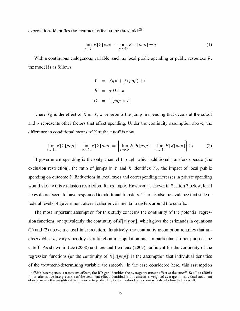
Table 2 shows descriptive statistics for the variables used in the statistical analysis, as well as
other information regarding revenue and expenditures in the municipalities. The numbers show
that FPM transfers are the most important source of revenue for the relatively small local govern-
18

ments considered here, amounting to about 50% on average and 56% in rural areas. Table 2 also
shows that education spending accounts for about 20% of local budgets on average, with similar
shares going to housing and urban infrastructure, and transportation spending. In addition, Table 2
documents a marked difference in development indicators between the relatively developed south-
ern part of the country (South, Southeast and Center-West regions) and the less developed northern
regions (North and Northeast region, see Table 2 for de�nitions). The contrast between rural and
urban communities is similarly striking.
5 Estimation approach
Following Hahn, Todd, and Van der Klaauw (2001) and Imbens and Lemieux (2008), the main
estimation approach is to use local linear regression in samples around the discontinuity, which
amounts to running simple linear regressions allowing for different slopes of the regression func-
tion in the neighborhood of the cutoff. Allowing for slope is particularly important in the present
application because per capita transfers are declining as population approaches the threshold from
below, and again declining after the threshold. Assuming that a similar pattern characterizes out-
comes as a function of population, a simple comparison of means for counties above and below the
cutoff would provide downward biased estimates of the treatment effect. I follow the suggestions
by Imbens and Lemieux (2008) and use a rectangular kernel (i.e. equal weight for all observations
in the estimation sample).
Because there are relatively few observations in a local neighborhood of each threshold, I also
makes use of more distant municipalities. The disadvantage of this approach is that the speci�-
cation of the function f .pop/, which determines the slopes and curvature of the regression line,
becomes particularly important. To ensure that �ndings are not driven by functional form assump-
tions, I present most estimation results from linear speci�cations in the discontinuity samples,
adding quadratic speci�cations as a robustness check. I supplement the local linear estimates with
higher order polynomial speci�cations, using an extended support, and I choose the order of the
polynomial such that it best matches the local linear estimates in the discontinuity samples. This
approach thus combines the advantage of local linear regression�comparing municipalities close
to the cutoff, where local randomization of the treatment is most likely to hold but the variance of
19

the estimates is relatively high�with the main advantage of using an extended support, namely
sample size, which helps to reduce standard errors.
In the analysis that follows, I focus particularly on the �rst three population cutoffs (c1 D10'188,
c2 D13'584, and c3 D16'980). At subsequent cutoffs the variation in FPM transfers is too small
to affect municipal overall budgets, and hence there is no "�rst stage" in terms of overall resources
available for the municipality, as shown in Section 7 below. While I present results for the �rst three
cutoffs individually, I also pool the municipalities across these cutoffs in order to gain statistical
power.
Pooling requires the treatment intensity to be of comparable magnitude in order to interpret the
size of estimated impacts.27 As discussed above, although the funding jump is about 1'320'000
Reais (2008 prices) or about 1'000'000 international US$ at each cutoff, the treatment in terms
of additional per capita funding is not the same across cutoffs. However, the differences across
the �rst three cutoffs are not that large, and since there are likely to be economies of scale in
the provision of local public services�that is, unit costs decline with scale�the differences in
treatment across cutoffs are likely even smaller than what the differences in per capita funding
jumps suggest. With similar treatment intensity it seems reasonable to expect similar treatment
effects at least around the �rst few cutoffs, a testable hypothesis for which I �nd support below.
The speci�cation I use to test the null hypothesis of common (average) effects across the �rst
three cutoffs is as follows. Let seg j denote the four integers (7'500, 11'800, 15'100, and 23'772)
that bound and partition the population support into three segments; Yms an outcome in munici-
pality m, state s; zms a set of pre-treatment covariates; as a �xed effect for each state; and ums an
error term for each county. Neither covariates nor state �xed effects are needed for identi�cation.
I include them to guard against chance correlations with treatment status and to increase the preci-
sion of the estimates. The testing speci�cation for a given percentage distance p from the cutoffs27Treatment effects need not be the same across cutoffs. If treatment effects are heterogeneous, the pooled estimatesidentify an average treatment effect across cutoffs.
20

is then:
Yms D�� 11[popms > c1]C �10 popms C �11.popms � c1/1[popms > c1]
�11p
C�� 21[popms > c2]C �20 popms C �21.popms � c2/1[popms > c2]
�12p
C�� 31[popms > c3]C �30 popms C �31.popms � c3/1[popms > c3]
�13p
C3PjD1� j1[seg j�1 < popms � seg j ]1 j p C zms C as C ums
seg0 D 7500; seg1 D 11800; seg2 D 15100; seg3 D 23772
1 j p D 1[c j .1� p/ < popms < c j .1C p/]; j D 1; 2; 3I p D 2; 3; 4%
Figure 2 illustrates the estimation approach. I fail to reject the null hypotheses � 1 D � 2 D � 3 at
conventional levels of signi�cance for all outcomes and in all speci�cations.
For the pooled analysis, I need to make observations comparable in terms of the distance from
their respective cutoff. To do this, I rescale population to equal zero at the respective thresholds
within each of the �rst three segments, and then use the scaled variable, Xms (municipality m in
state s), for estimation purposes:
Xms D popms � 10188 if seg0 < popms � seg1
popms � 13564 if seg1 < popms � seg2
popms � 16980 if seg2 < popms � seg3
Yms D �1[Xms > 0]1p C [�10Xms C �11Xms1[Xms > 0]] 11p (3)
C [�20Xms C �21Xms1[Xms > 0]] 12p
C [�30Xms C �31Xms1[Xms > 0]] 13p
C3PjD1� j1[seg j�1 < popms � seg j ]1 j p C zms C as C ums
1p D 11p C 12p C 13p
Essentially this equation allows for six different slopes, one each on either side of the three cut-
21

offs, but imposes a common effect � . Under the continuity assumption above, the pooled treatment
effect is given by lim1#0
E[Y jX D 1] � E[Y jX D 0] D � . Both the pooled treatment effect and
effects at individual cutoffs are estimated using observations within successively larger neighbor-
hoods (larger p) around the cutoff in order to assess the robustness of the results.
6 Internal validity checks
Since extensive manipulation of the population �gures on which FPM allocations were based
would cast serious doubts on the internal validity of the design, I check for any evidence of sort-
ing, notably discontinuous population distributions. Figure 4 plots the histogram for 1982 of�cial
municipality population.28 The bin-width in this histogram (283) is set to ensure that the various
cutoffs coincide with bin limits. That is, no bin counts observations from both sides of any cutoff.
Visual inspection reveals no discontinuities and the null hypothesis of a smooth density cannot be
rejected anywhere near conventional signi�cance levels for any of the �rst six cutoffs according to
the density test suggested by McCrary (2008).29
In Table 3, I estimate equation (3) pooled across the �rst three cutoffs for a host of pre-treatment
outcomes and other covariates. The results show that, in the samples with population of +/- 2 or
3 percentage points around the cutoffs, there is no statistical evidence of discontinuities in the
1980 pre-treatment covariates mentioned above. Nor is there statistical evidence of pre-treatment
differences in the total public budget or its main components. While the 1981 public �nance reports
do not disaggregate transfers into FPM transfers and other categories, FPM transfers represent the
bulk of current transfers, and so any discontinuities in pre-treatment FPM transfers should show
up in 1981 current or capital transfers. Table 3 shows that such is not the case.
In the larger samples that include municipalities within +/- 4 to 6 percentage points, some in-
dividual discontinuities in Table 3 are statistically signi�cant. This happens mostly due to larger
point estimates compared to the smaller bandwidths, rather than lower standard errors, which sug-
gests that these signi�cant results might re�ect a speci�cation error.30 Table 3.1 in the Online28The histogram for the full support is omitted to save space and available upon request.29The estimates (and standard errors) are, for the �rst to sixth cutoffs respectively, -0.085 (0.098), -0.002 (0.112), 0.152(0.135), 0.071 (0.167), -0.041 (0.253), 0.324 (0.344). Separate density plots for each cutoff are presented in Figure 4.1 inthe Online Appendix.30See for example Lee and Lemieux (2009) for more discussion on this point.
22

Appendix shows results from quadratic speci�cations that con�rm this view: virtually none of the
pre-treatment differences found in the 4 and 5 percent samples in Table 3 are now statistically sig-
ni�cant, due to both lower estimates and higher standard errors. Moreover, all F-tests in Tables 3
and 3.1 fail to reject the joint null hypotheses of no discontinuities in any pre-treatment covariate
at conventional levels of signi�cance (lowest p-value is 0.26).31 In other words, from a statistical
point of view, there is no evidence that treatment group municipalities were systematically differ-
ent in terms of local development or overall public resources from municipalities in the marginal
comparison group in the pre-treatment period.32
Nonetheless, the point estimates for education outcomes and public revenues are all positive.
Moreover, some of these estimates are of the same order of magnitude as those found in the post-
treatment period as further discussed below, suggesting that treatment group municipalities might
already have been somewhat better off than those in the comparison group as of 1980. In Section
7 below I show that the estimated effects are robust to the inclusion of relevant pre-treatment
covariates, including the four pre-treatment education and earnings outcomes shown in Table 3.
In Section 8, results are shown to be robust to a difference-in-differences approach that directly
controls for pre-treatment schooling differences of elementary-school-age cohorts.
7 Main estimation results
This section starts out by demonstrating that FPM transfers increased local total revenue and spend-
ing per capita by about 20%, with no evidence of crowding out own revenue or other revenue
sources. Local spending shares remained essentially unchanged, that is, local spending on educa-
tion, housing and urban infrastructure, and transportation all increased by about 20% per capita.
The second subsection presents direct evidence on public service improvements in these broad
spending areas. The third subsection discusses the main empirical result of the paper which is that
communities that received extra �nancing from the central government bene�ted in terms of edu-
cation outcomes (higher schooling and literacy rates). The fourth subsection presents and discusses
effects on income (lower poverty rates). The �nal subsection shows that the estimated impacts are31The test of the joint null hypotheses of no jumps in pre-treatment covariates is done by stacking these variables andrunning a joint estimation of individual discontinuities (Lee and Lemieux, 2009).32Results for the �rst two cutoffs pooled are quantitatively similar and available upon request.
23

not only individually but jointly signi�cant.
All the tables below show results for the �rst two cutoffs pooled and the �rst three cutoffs
pooled, as well as for the cutoffs individually. The tables present results for successively larger
samples around the cutoffs (p D 2; 3; 4;and 15%) and for each sample with and without covariates.
The discussion will focus on the pooled estimates because F-tests fail to reject the null hypothesis
of homogenous effects at the three cutoffs at conventional levels of signi�cance for all outcomes
and in all speci�cations. Among the pooled estimates, those that control for covariates (including
pre-treatment outcomes) are the most reliable because they control for chance correlations with
treatment status. They are also the most precisely estimated, because the covariates absorb some
of the variation in the outcome measures.
7.1 Effects on overall spending and spending shares
Table 4 gives estimates of the jump in total local public revenue per capita over the 1982-1985
period. The pooled estimates in the �rst two rows suggest that per capita revenues increased by
about 20 percent at the thresholds. The magnitude of the jump is roughly consistent with the size
of FPM transfers in local budgets (about 50%) and the jump in per capita FPM transfers at the
cutoffs (about 33% for the 10'188 cutoff and less for subsequent cutoffs).33 Figure 4 graphically
represents the results for FPM transfers, total revenue, own revenue and other revenues, which are
composed of other federal and state government transfers, all cumulative over the period 1982-
1985. Each dot represents the residual from a regression of the dependent variable on state and
segment dummies averaged for a particular bin. The state and segment effects are included to
absorb some of the variation in the dependent variable and make the jump at the cutoff more easily
visible. For example, the �rst dot to the left of zero in panel B of Figure 4 represents average
residual total government revenue per capita for all municipalities within one percentage point (in
terms of population) to the left of one of the �rst three population thresholds.34
33To see this, let R denote total revenue, F FPM funding and O other funding, such that R D F C O and 1RR D
1FFFRC
1OO
OR . If1O D 0, as shown below, and
FR D 0:5 on average, as shown in Table 2, then
1RR D 33%�50% D 16:5%:
The estimates in Table 4 are somewhat larger, perhaps because municipalities with missing FPM information rely moreheavily on FPM funding, in which case FR might be more like 0:6, or simply by chance. Note that proportional changes atthe cutoff are identical whether or not the variable is scaled by population, P: 1 ln
� RP�D 1 ln.R/ �D 1R
R .34The null hypothesis that population means are equal for two sub-bins within each bin cannot be rejected, suggestingthat the graph does not oversmooth the data (Lee and Lemieux 2009).
24

To demonstrate the correspondence between panel B of Figure 4 and the results in Table 4, if
instead of �tting two straight regression lines through the ten dots on either side of the cutoff, this
�gure were to �t two lines through the �rst two dots on either side of the cutoff, the result would
roughly illustrate the jump estimated in column 1 of Table 4 for pooled cutoffs 1-3 in the two
percent neighborhood without covariates. With this in mind, the �gure shows clear evidence of
a discontinuity in total per capita revenue at the pooled cutoff, and it additionally shows that the
discontinuity is visually robust irrespective of the width of the neighborhood examined. It is also
worth noting that both the regression functions for total revenue per capita and FPM per capita
(panel A) slope downward, to the left and to the right of the cutoff, as expected given the FPM
allocation mechanism.
At the same time, panels C and D of Figure 4 show that there are no discontinuities in either
own revenue or other revenues. This suggests that the effects on education and poverty discussed
below can be attributed to local spending on public services, rather than additional private spending
associated with local tax breaks (that is, the exclusion restriction discussed in Section 3 seems to
hold). Statistical analysis con�rms this conclusion but is not presented here to save space (results
are available on request). Table 5 shows that total spending increased by an almost identical per-
centage as total revenue. Because small local governments were running close to balanced budgets
at the time, this implies that total spending increased essentially one-for-one with FPM transfers.35
This result is also borne out when I estimate the effect of FPM funding per capita on total per capita
spending directly, using the treatment indicator I [X > 0] as the instrument. Estimates are almost
always at 1 or above, statistically different from zero, and virtually never statistically different from
unity as shown in Table 5.1 in the Online Appendix.
Tables 4 and 5 also show that for larger municipalities around the 4th cutoff, the increase in
FPM transfers was too small to affect their overall budget, and hence there was no "�rst stage" in
terms of overall resources.36 One could argue that the 4th cutoff could be used as well because,
although not signi�cant, the point estimates are similar to those at preceding cutoffs. While this is35To see this, let R denote total revenue as before, Exp; total expenditures and B the budget balance, such that R DExp C B and 1R
R D 1ExpExp
ExpR C 1B
BBR . If the budget is balanced, B D 0, then
1RR D 1Exp
Exp implies that every Real ofextra revenue was spent. But if B > 0 for example, we could �nd 1R
R D 1ExpExp and yet part of the extra revenue would
have been saved or used to pay back debt.36At the 5th cutoff the discontinuity estimates are much more variable and they are nowhere near statistical signi�cance.Results are available on request.
25

a sensible argument, estimates around higher cutoffs are not pursued here for the sake of brevity
and ease of interpretation of the estimated impacts (see Section 7.3 below). Another point worth
noting is that the included pre-treatment covariates are signi�cant predictors of municipality per
capita revenue and spending, thus lowering standard errors. Pretreatment covariates also seem to
be weakly related to the treatment indicators although the change in point estimates is relatively
minor.
Figure 5 documents effects on total spending per capita as well as on the main local expenditure
categories: education, housing and urban infrastructure, and transportation. As with total revenue,
there is clear evidence of a jump of about 20% at the cutoff in all of these variables, although the
jumps in expenditure categories are nowmore sensitive to the width of the neighborhood examined.
The regression lines also slope downward almost without exception, which is further evidence
favoring the validity of the design. The spending category graphs are considerably noisier than the
total spending graph because the sample size is smaller (due to missing values) and because the
expenditure categories are only available for the years 1982 and 1983, whereas total spending is
reported over the entire period 1982 to 1985. Nevertheless, the jumps in the expenditure categories
are also statistically signi�cant as shown in Table 6. This evidence thus suggests that local spending
on education, housing and urban infrastructure, and transportation all increased by about 20% per
capita, leaving local spending shares essentially unchanged.37
7.2 Effects on public services
Having established that additional FPM transfers were used to �nance an expansion of public
spending per capita of about 20% over the period 1982-1985, the remainder of this section proceeds
to document impacts of this extra spending on public services.
Table 7 shows effects on the primary school teacher-student ratio. Although the extra FPM
funding stopped by the end of 1985, effects on teacher-student ratios in 1991 might arise if the
extra spending on education was in fact smoothed over subsequent years or if additional teachers
could not easily be dismissed. Estimates are reasonably close across samples and suggest that the
teacher-student ratio increased by about .01, or one teacher per hundred students. This compares37To be precise, the null hypothesis of a proportional, 20 percent per capita increase cannot be rejected in any of thespeci�cations.
26

to an average teacher-student ratio in the marginal comparison group of about .05. The implied
average class-size reduction at the primary school level amounts to about 3 students per teacher.
In contrast, results on municipal elementary schools (not shown) display no clear patterns and are
imprecisely estimated, suggesting that transfers �nanced mostly more labor input as opposed to
school infrastructure.
Housing infrastructure measures do not indicate much evidence of public service improvements
although they are for the most part positive and also statistically signi�cant in some speci�cations.
Rather than showing separate tables with mostly insigni�cant results, I present the school and
housing infrastructure estimates below when I test the joint signi�cance of all the outcome vari-
ables. Figure 6 shows the results for the teacher-student ratio, elementary schools, and water and
electricity access graphically (the graphs for sewer and inadequate housing look very similar to the
electricity graph). Direct evidence on public service improvements is thus mixed at best: while
there is evidence that student-teacher ratios in local primary school systems fell, there is little
evidence that housing and urban development spending affected housing conditions.
7.3 Effects on education outcomes
This section presents estimates of education and income gains for the communities that received
extra �nancing from the central government. Tables 8 and 9 present results for average years
of schooling (completed grades) of individuals 19 to 28 years and 9 to 18 years of age in 1991,
respectively. The pooled point estimates in rows 1 and 2 of Table 9 suggest that the older cohort
accumulated about 0.3 additional years of schooling per capita (speci�cations with covariates).
This schooling gain would be consistent with 3 out of 10 individuals from this cohort completing
an additional year of schooling for example. The estimates at individual cutoffs are all positive
but more variable, which likely re�ects small sample biases. While most of the estimates from
individual cutoffs are not signi�cantly different from zero, the pooling across cutoffs c1 and c2, as
well as c1; c2 and c3, yields statistically signi�cant estimates (at 1%) even within a relatively small
neighborhood of +/- 3% around the cutoffs.
Corresponding results for the younger cohort shown in Table 9 suggest a schooling gain of about
0.15 years per capita. Pooled estimates are again mostly signi�cantly different from zero even in
27

the discontinuity samples. Given that average years of schooling in marginal comparison group
counties for the 19-28 aged cohort in 1991 was about 4.3 years with a standard deviation of 1.45
years, the schooling gains amount to about 7% or about 0.2 standard deviations. For the younger
cohort, the marginal comparison group years of schooling were 2.7 years with a standard deviation
of 1.08 years. The 0.15 schooling gain thus amounts to about 6% or 0.14 standard deviations.
It is important to note that the 4.3 average years of schooling for the older cohort represents
grades completed, not "years in school". We do not know how many years the cohort 19-28 in
1991 (10-19 in 1982) spent in school, but it should be at least 8 because schooling is compulsory
for children aged 7-14 years. On average in Brazil at the time, a year in school led to about 0.625
completed grades�5 years of completed grades for 8 years in school�which is consistent with the
4.3 years of schooling we �nd in the comparison municipalities (World Bank, 1985). In addition
to the 10- to 14-year-olds in 1982, years of schooling might also have increased because of the
cohorts aged 15 through 18 who were still eligible for elementary school. Even most of the 19-
year-olds on September 1st in 1982 (28 in 1991), the last cohort included in the analysis, were
18 years old at some point during 1982 and hence could have bene�ted from improvements in the
elementary school system.
In order to interpret these results, it is useful to consider the marginal cost of a year of schooling
implied by these estimates and compare it to the average cost of schooling in Brazil at the time.
This requires some assumptions, but a rough comparison can be made. The cumulative (1982-
1985) jump in per capita funding averaged across the �rst three cutoffs is about 100 R$ expressed
in 2008 prices, or 71 international US$.38 Assuming that about 20% of the additional FPM funds
were spent on education (Table 6), and assuming further that only the 0- to 18-year-olds in 1982,
about 50% of the total population,39 were at least marginally affected by the spending boom,
marginal education spending per student was about $71� 0:2� 2 D $28:4. According to Tables 8
and 9, this marginal spending purchased about 0.3 years and 0.15 years of schooling (speci�cations
with covariates), respectively. Taking an unweighted average of 0.225, the implied marginal cost of38Note that the 100R$ jump is averaged over three treatment intensities, namely 78R$, 97R$ and 130R$ per capita. Thecalculations below use this "average extra funding" which roughly corresponds to funding received by municipalities atthe second cutoff. Adding more dissimilar funding jumps would further complicate the interpretation of estimated impactsbased on pooled speci�cations.39Census tabulations in De Carvalho (1997).
28

an additional completed year of schooling is about $28:4� 10:225 D $126. This compares to average
annual education expenditures per capita at the cutoffs in 1982 of about 44 R$ in 2008 prices, or 31
international US$. Assuming again that these funds were spent on the 0- to 18-year-olds, and that a
year in school leads to about 0.625 completed grades on average (World Bank, 1985), the average
cost of a completed additional year of schooling is about $31� 2� 10:625 D $99. While these are
rough estimates, the similarity of the marginal cost to the average cost indicate that the �ndings
here are certainly plausible. Moreover these estimates suggest that�accounting for corruption and
other leakages�providing more �nancing to local governments at the margin improved education
outcomes at reasonable cost.
Tables 10 and 11 show that students not only completed more grades in municipalities that
received extra funds but that for some of them it made the difference between being able to read
and write or not. For the older cohort the effect on literacy amounts to about 4 percentage points,
compared to an average literacy rate of about 76% in the comparison group. For the younger
cohort the literacy differential is about 3 percentage points compared to an average literacy rate of
about 74% in the comparison group. Panels A and B of Figure 7 show the schooling and literacy
results for the older cohort graphically (the graphs for the younger cohort are omitted to save space
and are available on request). In line with this graphical evidence, estimates of the discontinuity
for neighborhoods not shown in Tables 8 through 12 are quantitatively similar to the estimates
presented here and are available upon request.
7.4 Effects on poverty and income per capita
Both better and more widespread education and better local public service quality overall (better
infrastructure and primary health care for example) are likely to increase household incomes. The
evidence suggests that the extra public spending indeed had an effect on income, although only for
the poor. Speci�cally, Table 12 shows impacts on the municipality poverty rate (measured relative
to the national income poverty line). All pooled estimates shown in rows 1 and 2 are negative, with
values around -4 to -5 percentage points, down from a mean poverty rate of 64% in the comparison
group. The estimates at individual cutoffs are also all negative although they are more variable.
While most of the estimates from individual cutoffs are not signi�cantly different from zero, the
29

pooling across cutoffs yields statistically signi�cant estimates (at 1%) even in the discontinuity
samples. While income per capita in 1991 is higher in the communities that got more funding,
the difference is not statistically signi�cant (results not shown). Panels C and D of Figure 7 show
effects on the poverty rate and on household income per capita graphically.
In order to interpret the results on poverty reduction, it is again useful to do some back-of-the-
envelope calculations. As emphasized in Section 3, impacts on poverty are likely to arise through
better and more widespread education, as well as through better local public service quality overall
(better infrastructure and primary health care for example). Regarding the education channel,
Tables 8 and 9 show that the schooling gains for the 10- to 19-year-olds and the 0- to 9-year-olds in
1982 were 0.3 years and 0.15 years, respectively. A likely distribution of individual-level gains that
would lead to this average impact is that 30 out of 100 individuals in the older cohort and 15 out of
100 in the younger cohort completed another year of schooling. Given the shares of these cohorts
in the total population�27% and 23%, respectively, according to De Carvalho (1997)�we can
thus estimate what percent of the overall population got an additional year of schooling, namely
about 27%� 15%C 23%� 30% D 11%.
Now suppose that an extra year of schooling raises wages by 12% (Behrman and Birdsall 1983),
that labor supply is constant, and that about 10% of the population earn per capita income that falls
within a 12% range below the poverty line. Suppose further that about 64% of the total population
would have been poor in the absence of the extra funding (this corresponds to the comparison
group average poverty rate shown in Table 12) and that schooling only increased among the poor,
so that 0:11=0:64 D 17:2% of the poor got an additional year of education. If the schooling gains
are independent from the distance to the poverty line, then 10% � 17:2% D 1:72% of the total
population escaped poverty through the schooling channel alone. This number will be higher the
larger the (average) returns to schooling, the larger the share of the population within range to
cross the poverty line given returns to schooling, and the higher the share of the poor within that
range that do get an additional year of schooling (those closer to the poverty line might be more
likely to get more schooling than those that are extremely poor). The education channel alone can
thus account for about 2 percentage points of the estimated total 4-5 percentage points of poverty
reduction, leaving the remaining 2 to 3 percentage points to better local public service quality
30

overall.
7.5 Testing joint signi�cance
The analysis so far has examined the effects of additional �nancing on several intermediary and
�nal outcomes, some of which were statistically signi�cant, while others were not. Since exam-
ining a suf�cient number of variables would always yield some that are statistically different from
zero simply by chance, it is important to test the joint hypotheses of zero effects in all variables.
Table 13 presents local linear estimates from the pooled speci�cation across the �rst 3 cutoffs and
the results of F-statistics, testing the null hypothesis of no discontinuities in any outcome variable.
The tests clearly reject these joint hypotheses, suggesting that at least some of the effects are real.
Overall there is thus strong evidence that the additional public spending improved education
outcomes at reasonable cost and reduced the number of poor people relative to the national income
poverty line. It is worth remembering at this point that�under the continuity assumption and
exclusion restriction discussed in Section 5 above�these effects can be attributed to extra local
public spending (although not exclusively to education spending), rather than private spending,
since there is no evidence of local tax breaks, and direct welfare spending by local governments
was very limited.
8 Further robustness checks
This section provides further robustness checks regarding functional form of both the running
variable (population) and of pre-treatment covariates, as well as difference-in-differences estimates
that directly control for pre-treatment schooling differences of elementary-school-age cohorts. The
corresponding difference-in-differences estimates are also presented for cohorts that have largely
completed their education and for whom one would expect smaller or no impacts. A �nal robust-
ness check uses only the sub-sample of individuals who were born in the municipality and never
moved away. The section starts out with robustness checks for schooling (8.1), followed by literacy
(8.2) and poverty (8.3). All the previously discussed results turn out to be robust to these additional
tests. The corresponding tables are available in an online appendix.
31

8.1 Schooling
Table 8.1 presents pooled estimates across cutoffs c1 and c2, as well as c1; c2 and c3 for the older
cohorts of 19- to 28-year-olds in 1991 and for the three previously used bandwidths (p D 2%; 3%
and 4%). For each bandwidth Table 8.1 has 3 columns, corresponding to the following speci�-
cations: �rst, linear population polynomial with pre-treatment covariates as in Table 8 but now
including average years of schooling of the 8- to 17-year-olds in 1980 (19- to 28-year-olds in
1991) based on the 1980 census micro-data as an additional control; second, quadratic population
polynomial without covariates; and third, linear population polynomial with a quadratic speci�-
cation of the pre-treatment covariates. The corresponding results for the younger cohort of 9- to
18-year-olds in 1991 are presented in Table 9.1.
All estimates in Table 8.1 are positive and most of them fall in the 0.2 to 0.3 range, the same
result encountered in Table 8 for the speci�cations with covariates. And as before, these estimates
become statistically signi�cant (at 5%) even within a relatively small neighborhood of +/- 3%
around the cutoffs. Table 8.1 also gives results of three hypothesis tests, one for each of the three
speci�cations discussed above. The �rst is a t-test of the hypothesis that the coef�cient on the pre-
treatment outcome is equal to one, as imposed in the �rst-difference speci�cation further discussed
below. This null hypothesis is soundly rejected across bandwidths and cutoffs (p-values of 0.01 or
lower). It turns out, however, that whether the coef�cient on initial schooling is imposed or not
matters little for the results. The second test investigates the joint hypotheses that the coef�cients
on the quadratic population terms on either side of the cutoff are zero, that is, whether linearity
of the population polynomial can be rejected. As expected, there is no statistical evidence against
linearity close to the cutoff (p D 2% and 3%) although for the p D 4% bandwidth linearity is
clearly rejected. The third is an F-test for the joint hypotheses that the coef�cients on the quadratics
in covariates are all zero. It turns out that the statistical evidence against including covariates
linearly is weak across bandwidths and cutoffs.
Estimates of the schooling gains for the 9- to 18-year-old cohort in 1991 based on the same
speci�cations as above are presented in Table 9.1. The only difference is that pre-treatment average
schooling for this cohort (0- to 7-year-olds in 1980) is not included since the census only collects
schooling information for those aged 5 or above. As in Table 9, the discontinuity estimates �uctuate
32

around 0.15 years per capita, again statistically signi�cant even in the narrow samples around the
cutoffs. Again there is no statistical evidence against linearity of the population polynomial close
to the cutoff .p D 2% and 3%) and only weak statistical evidence against including covariates
linearly.
Table 8.2 presents estimates of a difference-in-differences approach where the dependent vari-
able is the difference in average years of schooling between 1991 and 1980 of the older cohorts
(19- to 28-year-olds in 1991). This approach effectively controls for municipality-level unob-
served time-invariant factors that might be correlated with extra funding but imposes a coef�cient
of one on initial schooling of this cohort, rather than allowing the coef�cient to be estimated as
in Table 8.1 above. For each bandwidth Table 8.2 has 3 columns, corresponding to the following
speci�cations: �rst, linear population polynomial without covariates; second, quadratic population
polynomial without covariates; and third, linear population polynomial with covariates. Again,
all estimates in Table 8.2 are positive, most of them fall in the 0.2 to 0.3 range and they become
statistically signi�cant even within a relatively small neighborhood of +/- 3% around the cutoffs.
In contrast, the corresponding difference-in-differences estimates for those 25 years and older
in 1980�typically considered to have completed most of their schooling�are close to zero in
magnitude (sometimes negative) and very far from statistical signi�cance as shown in Table 8.3.
These estimates are for the exact same cohorts for which Table 3 shows a positive schooling dif-
ferential before the extra funding had started. While it is reassuring that these older cohorts did
not experience any schooling gains, strictly speaking this is not a placebo experiment. Although
one would expect smaller effects on education outcomes for cohorts that were beyond regular el-
ementary schooling age, the effect need not be zero since older cohorts might have attended adult
literacy programs that were promoted by the military government and offered through the local
administration, such as the MOBRAL (Movimento Brasileiro de Alfabetização). In fact the dif-
ference in average years of schooling of these cohorts in the comparison group is about 0.32, on
average (Table 8.3). This would be consistent with roughly one out of three individuals among
those 25 years and older getting an extra year of schooling over the eleven-year-period from 1980
to 1991.
As a �nal robustness check, I also estimate the impact on schooling for the 19- to 28-year-olds
33

in 1991 on a restricted sample of individuals who were born in a given municipality and never
moved away. The results are shown in Table 8.4 and are again quantitatively close to those from
the unrestricted sample. This provides suggestive evidence that the schooling gains stem at least
partly from existing residents, rather than being driven by in-migration of more highly educated
individuals in response to public service improvements. The results are only suggestive, however,
because there could be selective attrition among non-migrants across treatment and comparison
communities. In particular, more educated individuals might be more likely to stay in the munici-
pality in response to public service improvements.
8.2 Literacy
Tables 10.1 and 11.1 present robustness checks for literacy outcomes of the 19- to 28-year-olds
and 9- to 18-year-olds in 1991, respectively, using the same speci�cations as in Tables 8.1 and 9.1
above. As in Table 10, the estimates in Table 10.1 suggest a literacy gain of about four percentage
points throughout, signi�cant even in the +/- 2% window around the cutoffs. As with schooling
above, the hypothesis that the coef�cient on the pre-treatment outcome is equal to one is soundly
rejected across bandwidths and cutoffs (p-values of 0.00). And again as expected, there is no
statistical evidence against linearity of the population polynomial close to the cutoff (p D 2% and
3%) although for the p=4% bandwidth linearity is again rejected. There is also strong statistical
evidence across bandwidths and cutoffs against including covariates linearly. This turns out not to
matter much since estimates with linear vs. quadratic covariates are very similar if not identical.
Estimates of the literacy gains for the 9- to 18-year-old cohort in 1991 are presented in Table
11.1. As in Table 11, estimated impacts are all around three percentage points, again statistically
signi�cant even in the discontinuity samples. As in Table 10.1 there is no statistical evidence
against linearity of the population polynomial close to the cutoff and strong evidence against in-
cluding covariates linearly across bandwidths and cutoffs.
Table 10.2 presents estimates where the dependent variable is the difference in literacy rates
between 1991 and 1980 of the older cohorts (19- to 28-year-olds in 1991). Compared to the
estimates of about four percentage points in Tables 10 and 10.1, those in Table 10.2 suggest a
slightly lower literacy gain of about three percentage points, again statistically signi�cant even
34

within a relatively small neighborhood of +/- 3% around the cutoffs.
Table 10.3 presents the �nal robustness check for the literacy gains of the 19- to 28-year-olds
in 1991 based on the sub-sample of individuals who were born in a given municipality and never
moved away. The results are again quantitatively close to those from the unrestricted sample.
8.3 Poverty
Table 12.1 presents robustness checks for the poverty rate using the same speci�cations as in Table
8.1 above. As in Table 12, the estimates in Table 12.1 suggest a poverty reduction of about four to
�ve percentage points, signi�cant even in the +/- 2% window around the cutoffs. As with school-
ing and literacy above, the hypothesis that the coef�cient on pre-treatment poverty is equal to one
is soundly rejected across bandwidths and cutoffs (p-values of 0.00). There is no statistical evi-
dence against linearity of the population polynomial for any bandwidth. In contrast, there is strong
statistical evidence across bandwidths and cutoffs against including covariates linearly. Again, this
turns out not to matter much since estimates with linear vs. quadratic covariates are always very
similar if not identical.
9 Heterogeneous effects
In this section I show that additional resources had stronger effects on schooling and literacy in the
North of Brazil, which is generally less developed than the South (see Table 2 for the de�nitions of
North and South). In contrast, poverty reduction was evenly spread across the country. I also �nd
stronger effects on schooling in rural compared to urban municipalities, which would be consistent
with the larger role municipal governments play in the provision of elementary education in rural
areas.
Table 14 shows the effects of additional FPM transfers on total public spending per capita and
on the primary school teacher-student ratio in northern and southern states of Brazil. Spending
increased by about 20% in both parts of the country and effects on primary school teacher-student
ratios tend to be positive and statistically signi�cant, especially in the South. Although all estimates
tend to be larger in the South they are not statistically different from each other. None of the other
public service indicators are statistically signi�cant in either region (results not shown).
35

Table 15 shows that the average schooling and literacy gains reported earlier are for the most
part accounted for by gains in the northern part of the country. The estimates with covariates put
the schooling gains in the North at about 0.3 to 0.4 years. Literacy gains are also larger in the
North than in the South. These regional differences in literacy and schooling gains are statistically
signi�cant.40 The poverty reduction, in contrast, is larger in the South, although this difference is
not statistically signi�cant.
Tables 16 and 17 examine whether the notion that extra funds have stronger effects in less
developed areas holds true not just between the northern and southern parts of Brazil but also
across rural and urban areas as distinguished by the median percentage of urban residents in 1980.
Table 16 shows that spending increased by about 20% in both urban and rural municipalities. The
effect on primary school teacher-student ratios tends to be positive and statistically signi�cant in
rural areas, with no real difference in urban areas although the differential effect is not statistically
signi�cant.41 Again, none of the other public service indicators are statistically signi�cant in either
region (results not shown).
The results in Table 17 suggest that almost the entire schooling gains come from rural munici-
palities (an additional 0.5 year of schooling per capita). Effects in urban communities are smaller,
statistically insigni�cant and statistically different from the effects in rural communities.42 The lit-
eracy gains are more evenly spread although they too are concentrated among rural municipalities
and somewhat smaller in urban municipalities although the difference is not statistically signi�-
cant.43 The poverty reduction is evenly spread across urban and rural communities. Overall, these
results suggest that additional public spending had stronger effects on schooling and literacy in
less developed parts of Brazil, while poverty reduction was evenly spread across the country.44
An alternative explanation for these effects is that poor communities had stronger preferences
for education than richer communities and hence spent a higher proportion of extra funds on ed-
ucation. A direct test of this alternative view is to examine the share of education expenditure in40The coef�cients and standard errors on the interaction of the treatment indicator with the region indicator (1 for North)in the pooled sample for schooling and literacy are, respectively: 0.208 (0.105) and 0.019 (0.011).41The coef�cient and standard error on the interaction term of the treatment indicator with the urban indicator (1 forurban) are -.003 and (.004).42The coef�cient and standard error on the interaction term are -.185 and (.106).43The coef�cient and standard error on the interaction term are -.005 and (.011).44I also break the sample into high vs. low education and low vs. high initial poverty counties and �nd quantitativelysimilar results.
36

total spending subsequent to the increase in funding in poor vs. rich areas. Unfortunately, however,
existing expenditure data do not allow such a disaggregation between 1984 and 1989. When I test
for differential effects on education expenditure shares using data from 1982 and 1983, I �nd no
signi�cant effects (results not shown), suggesting that stronger preferences for education in poor
communities are not the driving force behind the higher schooling and literacy gains found in less
developed parts of Brazil.
10 Conclusion
Results presented in this paper suggest that communities that received extra �nancing from the
central government bene�ted in terms of education outcomes, used as an indirect summary mea-
sure of public service improvements. The implied marginal cost of schooling�accounting for
corruption and other leakages�amounts to about US$ 126, which turns out to be similar to the av-
erage cost of schooling in Brazil in the early 1980s. In turn, more education and better local public
service quality overall increased household incomes, although only for the poor. These effects can
be attributed to local public spending (although not exclusively to education spending), rather than
private spending, since there is no evidence of local tax breaks, and direct welfare spending by
local governments was very limited. It also seems that additional public spending had stronger
effects on schooling and literacy in less developed parts of Brazil, while poverty reduction was
evenly spread across the country.
As with any regression discontinuity analysis, the treatment effects presented in this paper apply
only to municipalities with population levels at the respective cutoffs. However, because results
are quantitatively similar across the �rst three thresholds it seems likely that the effects presented
here generalize at least to the subpopulation of municipalities in the approximate population range
8'500-18'700, which represents about 30% of Brazilian municipalities at the time. Whether pro-
viding additional �nancing to local governments in other contexts would yield similar results is an
open empirical question. The most closely related study on the effects of oil windfalls on local
spending and living standards in Brazilian municipalities �nds little if any effect on local public
services or household income per capita, although in some speci�cations they also �nd a reduction
in the poverty rate (Caselli and Michaels 2009).
37

Needless to say, the results presented in this paper do not imply that all is well with the way
public services are delivered in Brazil. The results do suggest, however, that even in the absence
of reforms that strengthen local accountability, and despite well founded worries about corruption,
other leakages, and local capture, local governments in Brazil did use the additional funds they re-
ceived to expand public services to the general local population at reasonable cost. Future research
might attempt to assess the relative magnitudes of leakage and service provision in (marginal)
government spending by looking at the exact services the money was spent on. Another important
question left unanswered here is what the effects of extra funding would be in a centralized system
without locally elected politicians. Given the scarcity of studies that trace the effects of funds on
spending to public services and into development outcomes, there is thus a lot of room for future
research.
38

11 References
Bandiera O., A. Prat and T. Valletti, 2009, �Active and Passive Waste in Government Spending:
Evidence from a Policy Experiment,� American Economic Review, 99: 1278-1308.
Banerjee, A., S. Jacob, M. Kremer, J. Lanjouw and P. Lanjouw, 2000, �Promoting School Partic-
ipation in Rural Rajasthan,� unpublished manuscript, MIT.
Bardhan, P. and D. Mookherjee, 2005, �Decentralizing antipoverty program delivery in develop-
ing countries,� Journal of Public Economics, 89: 675-704.
Behrman, J. R., and N. Birdsall, 1983, �The Quality of Schooling: Quantity Alone is Misleading,�
American Economic Review, 73(5): 928-946.
�,� and R. Kaplan, 1996, �The Quality of Schooling and Labor Market Outcomes,� in Bird-
sall N. and R. H. Sabot, editors, Opportunity Foregone: Education in Brazil, IADB, Johns
Hopkins University Press, 245-267.
Birdsall, N., 1985, �Public Inputs and Child Schooling in Brazil,� Journal of Development Eco-
nomics, 18: 67-86.
Bjoerkman, M. and J. Svensson, 2009, �Power to the People: Evidence from a Randomized Field
Experiment on Community-Based Monitoring in Uganda,� Quarterly Journal of Economics,
124(2): 735-769.
Bradford, D. F. and W. E. Oates, 1971, �The Analysis of Revenue Sharing in a New Approach to
Collective Fiscal Decisions,� Quarterly Journal of Economics, 85(3): 416-439.
Brollo F., Nannicini T., Perotti R. and G. Tabellini, 2010, �The Political Resource Curse,� NBER
Working Paper 15705.
Card, D. and A. B. Krueger, 1992, �Does School Quality Matter? Returns to Education and the
Characteristics of Public School in the United States,� Journal of Political Economy, 100:
1-40.
39

� and �, 1996, �School Resources and Student Outcomes: An Overview of the Literature and
New Evidence from North and South Carolina,� Journal of Economic Perspectives, 10(4):
31-50.
Carvalho, J. A. M. de 1997, �Demographic Dynamics in Brazil: recent trends and perspectives,�
Brazilian Journal of Population Studies, 1: 5-23.
Case, A. and A. Deaton, 1999, �School Inputs and Educational Outcomes in South Africa,�Quar-
terly Journal of Economics, 114(3), 1047-1085.
Caselli, F. and G. Michaels, 2009, �Do Oil Windfalls Improve Living Standards? Evidence from
Brazil,� unpublished manuscript.
Chin, A., 2005, �Can Redistributing Teachers Across Schools Raise Educational Attainment?
Evidence from Operation Blackboard in India,� Journal of Development Economics, 78: 384-
405.
Du�o, E., 2001, �Schooling and Labor Market Consequences of School Construction in Indone-
sia: Evidence from an Unusual Policy Experiment,� American Economic Review, 91(4):795-
813.
Easterly, W. R., 2006, The white man's burden: why the West's efforts to aid the rest have done
so much ill and so little good, Oxford. Oxford University Press.
��, ed., 2008, Reinventing foreign aid, Cambridge MA. MIT Press.
Ferraz, C. and F. Finan, 2008, �Exposing Corrupt Politicians: The Effects of Brazil´s Publicly
Released Audits on Electoral Outcomes,� Quarterly Journal of Economics, 123: 703-745.
Glewwe, P. and M. Kremer, 2006, �Schools, Teachers and Education Outcomes in Developing
Countries,� Handbook of the Economics of Education, Vol. 2.
��, ��, and S. Moulin, 2009, �Many Children Left Behind? Textbooks and Test Scores in
Kenya,� American Economic Journal: Applied Economics, 1(1): 112�35.
Hagopian, F. 1996, Traditional Politics and Regime Change, Cambridge University Press.
40

Hahn, J., P. Todd and W. Van der Klaauw, 2001, �Identi�cation and Estimation of Treatment
Effects with a Regression-Discontinuity Design,� Econometrica, 69: 201-209.
Hanushek, E. A., 2006, �School Resources,� Handbook of the Economics of Education, Vol. 2.
��, 1997, �Assessing the Effects of School Resources on Student Performance: An Update,�
Educational Evaluation and Policy Analysis, 19(2): 141-164.
Heckman, J. J., A. Layne-Farrar and P. Todd, 1996, �Does Measured School Quality Really Mat-
ter? An Examination of the Income-Quality Relationship,� in Burtless Gary ed., Does Money
Matter? The Effect of School Resources on Student Achievement and Adult Success, Wash-
ington, D. C., Brookings Institution, pp. 192-289.
Hines, J. R. and R. H. Thaler, 1995, �Anomalies: The Flypaper Effect,� Journal of Economic
Perspectives, 9(4): 217-26.
Hoxby, C. M., 2000, �The effects of class size on student achievement: New evidence from
population variation,� Quarterly Journal of Economics, 115(3): 1239-1285.
Imbens, G. and T. Lemieux, 2008, �Regression Discontinuity Designs: A Guide to Practice,�
Journal of Econometrics 142(2): 615-635.
Instituto Brasileiro de Geogra�a e Estatística, 2002, �Estimativas Populacionais do Brasil, Grandes
Regioes, Unidades da Federacao e Municípios,� IBGE background paper, Rio de Janeiro.
Krueger, A. B., 2003, �Economic Considerations and Class Size,� Economic Journal, 113: 34-63.
�� and D. M. Whitmore, 2001, �The Effect of Attending a Small Class in the Early Grades on
College-Test Taking and Middle School Test Results: Evidence from Project STAR,� Eco-
nomic Journal, 111: 1-28.
Lavy, V., 1996, �School supply constraints and children´s educational outcomes in rural Ghana,�
Journal of Development Economics, 51: 291-314.
Lee, D. S., 2008, �Randomized experiments from non-random selection in U.S. House elections,�
Journal of Econometrics 142(2): 675-697.
41

Lee, D. S. and T. Lemieux, 2009, �Regression Discontinuity Designs in Economics,� Journal of
Economic Literature, 48(2): 281-355.
Litschig, S., 2008, �Rules vs. political discretion: evidence from constitutionally guaranteed
transfers to local governments in Brazil,� Universitat Pompeu Fabra Working Paper 1144.
Litschig, S. and K. Morrison, 2012, �Government Spending and Re-election: Quasi-Experimental
Evidence from Brazilian Municipalities,� Universitat Pompeu Fabra Working Paper 1233.
Reinikka, R. and J. Svensson, 2004, �Local Capture: Evidence from a Central Government Trans-
fer Program in Uganda,� Quartely Journal of Economics, 199(2): 679-705.
Rodden, J. 2004, �Comparative federalism and decentralization: On meaning and measurement,�
Comparative Politics 36(4): 481-500.
Shah, A., 1991, �The new �scal federalism in Brazil,� World Bank Discussion Papers, 124, Wash-
ington, D.C.
� 2006, �A practitioner's guide to intergovernmental �scal transfers,� World Bank Policy Re-
search Working Paper 4039,Washington, DC: World Bank.
Van der Klaauw, W., 2002, �Estimating the Effect of Financial Aid Offers on College Enrollment:
A Regression Discontinuity Approach,� International Economic Review, 43(4): 1249�1287.
World Bank, 1985, Brazil: Finance of Primary Education, Washington D.C.
42

Table 1: Brackets and coef�cients for the FPM transfer
Population bracket Coefficientup to 10’188 0.6from 10’189 to 13’584 0.8from 13’585 to 16’980 1from 16’981 to 23’772 1.2from 23’773 to 30’564 1.4from 30’565 to 37’356 1.6from 37’357 to 44’148 1.8from 44’149 to 50’940 2from 50’941 to 61’128 2.2from 61’129 to 71’316 2.4from 71’317 to 81’504 2.6from 81’505 to 91’692 2.8from 91’693 to 101’880 3from 101’881 to 115’464 3.2from 115’465 to 129’048 3.4from 129’049 to 142’632 3.6from 142’633 to 156’216 3.8above 156’216 4Source: Decree 1881/81
43
Table 2: Descriptive statistics (sample means)
7'500 44'148 Sample Full Full North South Rural Urban
Observations 2306 1248 536 712 624 624
1980 county characteristics (IBGE)Average years of schooling (25 years and older) 1.96 1.90 1.04 2.56 1.52 2.29Percentage of residents living in urban areas (%) 30.0 27.9 22.4 32.2 14.8 41.7Net enrollment rate of 7 to 14yearolds (%) 55.6 55.5 39.5 67.6 48.9 62.1Illiteracy rate, 15 years and older (%) 39.0 39.1 56.0 26.3 44.4 33.7Poverty headcount ratio (national poverty line, %) 58.6 59.3 78.0 45.3 67.9 50.7Income per capita (% of minimum salary in 1991) 77.5 75.2 41.0 101.0 58.6 91.9Infant mortality (per 1000 life births) 88.9 88.5 129.0 57.6 96.2 80.7GDP ('000) 2008 Reais (IPEA) 108'587 64'214 33'023 87'728 46'827 81'741
1982 Financial data (Ministry of Finance)Total county revenue ('000) 2008 Reais 3'957 2'876 1'826 3'562 2'360 3'365Total county revenue 1982/GDP 1980 (%) 5.3 5.6 7.3 4.5 6.2 5.0FPM transfers/total revenue (%) 48.0 49.7 66.4 37.9 56.4 43.3Own revenue/total revenue (%) 5.9 5.1 1.1 7.7 2.6 7.5Other revenue/total revenue (%) 46.9 45.9 32.9 54.7 41.9 49.7Administrative spending/total spending (%) 22.3 22.3 22.9 21.7 21.8 22.9Education spending/total spending (%) 20.9 21.2 23.9 18.6 22.3 20.0Housing spending/total spending (%) 19.5 17.9 19.9 16.0 15.9 20.2Health spending/total spending (%) 9.9 10.4 14.3 6.3 11.1 9.6Transportation spending/total spending (%) 20.9 21.8 12.2 30.0 23.2 20.2Other spending/total spending (%) 8.5 8.5 8.5 8.5 8.2 8.6
1991 Real school resources (school census)Number of municipal elementary schools 37.8 30.2 41.0 20.0 37.5 21.4Primary school studentteacher ratio 20.3 19.7 22.5 17.1 20.4 18.9
1991 Housing and urban services (IBGE)Individuals with access to electricity (%) 71.0 70.0 52.4 83.3 58.2 81.9Individuals with access to drinking water (%) 70.0 69.4 50.0 83.8 62.2 76.5Individuals with access to sewer (%) 41.3 41.6 19.7 54.2 30.9 50.2Individuals living in inadequate housing (%) 0.61 0.53 0.62 0.47 0.46 0.62
1991 education outcomes (census)Average years of schooling (19 to 28yearolds) 4.6 4.5 3.33 5.5 4.0 5.1Literacy rate (19 to 28yearolds) (%) 78.8 79.0 63.0 91.1 73.7 84.3Average years of schooling (9 to 18yearolds) 2.8 2.9 1.8 3.6 2.5 3.2Literacy rate (9 to 18yearolds) (%) 76.8 77.2 57.8 91.9 71.1 83.4
1991 Household income (IBGE)Poverty headcount ratio (R$140 poverty line) (%) 60.0 60.2 80.0 45.3 69.2 51.2Household income per capita 2008 Reais 224 217 116 294 169 266
8'500 18'700 Population range
Notes : North includes North and Northeast regions, South includes CenterWest, Southeast and South regions. North region:Acre, Amazonas, Para, Amapa, Rondonia, Roraima states; Northeast region: Maranhao, Piaui, Ceara, Rio Grande do Norte,Paraiba, Pernambuco, Alagoas, Sergipe, Bahia states; CenterWest region: Mato Grosso, Mato Grosso do Sul, Goias states;Southeast region: Minas Gerais, Espirito Santo, Rio de Janeiro, Sao Paulo states; South region: Parana, Santa Catarina, RioGrande do Sul states. Rural sample: percentage of municipality residents living in urban areas < 24.8; Urban sample: percentage ofmunicipality residents living in urban areas > 24.8.
44

Table 3: Test of discontinuities in pre-treatment covariates
Polynomial specification: Linear Linear Linear Linear Linear
Neighborhood (%): 2 3 4 5 6
Opposition party (0/1) 0.131 0.078 0.049 0.056 0.061(0.108) (0.092) (0.082) (0.072) (0.066)
Average years of schooling 0.057 0.173 0.202* 0.231** 0.159*(25 years and older) (0.174) (0.137) (0.117) (0.108) (0.094)
Urban residents (%) 0.005 0.007 0.004 0.004 0.015(0.045) (0.036) (0.031) (0.029) (0.025)
Net enrollment rate (%) 2.060 3.382 4.595* 4.260** 2.076(7 to 14yearolds) (3.821) (2.891) (2.403) (2.133) (1.890)
Illiteracy rate (%) 1.146 1.511 2.638 2.886 1.794(15 years and older) (3.157) (2.286) (1.951) (1.782) (1.587)
Poverty headcount ratio (%) 3.895 0.563 1.523 2.077 0.186(National poverty line) (3.733) (2.868) (2.439) (2.227) (1.948)
Income per capita (%) 0.031 0.029 0.045 0.062 0.030(percent of minimum salary) (0.082) (0.059) (0.049) (0.045) (0.040)
Infant mortality 2.263 3.776 6.490 3.910 3.530(per 1000 life births) (5.406) (4.506) (4.111) (3.493) (3.221)
Log current transfers 1981 0.090 0.067 0.081 0.068 0.007(per capita) (0.093) (0.071) (0.065) (0.061) (0.056)
Log capital transfers 1981 0.027 0.097 0.097 0.062 0.064(per capita) (0.163) (0.130) (0.127) (0.109) (0.099)
Log total revenue 1981 0.085 0.080 0.130** 0.109* 0.050(per capita) (0.089) (0.072) (0.062) (0.057) (0.052)
Log own revenue 1981 0.498 0.464 0.411 0.348 0.299(per capita) (0.414) (0.315) (0.258) (0.232) (0.215)
Municipalities 200 293 386 471 561
Fstatistic[pvalue]
0.85[0.60]
0.80[0.65]
1.22[0.26]
1.16[0.31]
1.23[0.26]
Notes: Table entries are OLS estimates (standard errors) of discontinuities in pretreatment covariatesusing the pooled specification across the first three cutoffs described in Section 5, equation (3) in the maintext. Fstatistic tests the joint null hypotheses of no discontinuities in any pretreatment covariate.Clustered (at the municipality level) standard errors in parentheses. Neighborhood (%) is % distance fromrespective cutoff. All specifications include state fixed effects and segment dummies. All specificationsallow for differential slopes by segment and on each side of the cutoff. Opposition party is an indicator forwhether the county was run by a PDS mayor from 19821988 (0) or a mayor from an opposition party(PMDB, PDT, PT or PTB) (1). (***, **, and *) denote significance at the 1%, 5% and 10% levels,respectively.
45

Table 4: Impact on total revenue
Dependent variable: log total revenue per capita (19821985)
Polynomial specification: Linear Linear Linear Linear Linear Linear Various1
Neighborhood (%): 2 2 3 3 4 4 15
Pretreatment covariates: N Y N Y N Y Y
Pooled cutoffs 13I[X > 0] 0.146* 0.192*** 0.171*** 0.167*** 0.199*** 0.179*** 0.160***
(0.077) (0.071) (0.061) (0.053) (0.056) (0.050) (0.037)Observations 176 173 252 249 332 328 1041Rsquared 0.75 0.85 0.72 0.82 0.65 0.78 0.75
Pooled cutoffs 12I[X > 0] 0.169* 0.256*** 0.207** 0.217*** 0.202*** 0.193*** 0.210***
(0.102) (0.086) (0.082) (0.072) (0.075) (0.067) (0.048)Observations 116 115 173 172 222 220 711Rsquared 0.73 0.84 0.73 0.82 0.70 0.81 0.76
1st cutoffI[pop > 10188] 0.143 0.320** 0.255** 0.267** 0.233** 0.223** 0.256***
(0.154) (0.155) (0.113) (0.112) (0.101) (0.099) (0.085)Observations 58 57 88 87 117 115 386Rsquared 0.86 0.91 0.86 0.91 0.81 0.87 0.80
2nd cutoffI[pop > 13584] 0.148 0.195 0.205 0.291** 0.218* 0.282** 0.153**
(0.182) (0.180) (0.135) (0.142) (0.123) (0.124) (0.060)Observations 58 58 85 85 105 105 325Rsquared 0.67 0.82 0.67 0.80 0.67 0.81 0.75
3rd cutoffI[pop > 16980] 0.045 0.036 0.008 0.044 0.095 0.096 0.084*
(0.133) (0.102) (0.114) (0.080) (0.113) (0.069) (0.047)Observations 60 58 79 77 110 108 330Rsquared 0.86 0.95 0.82 0.92 0.63 0.81 0.76
4th cutoffI[pop > 23772] 0.023 0.142 0.088 0.093 0.202 0.102 0.096
(0.258) (0.131) (0.203) (0.164) (0.147) (0.118) (0.081)Observations 39 39 62 61 89 88 302Rsquared 0.90 0.96 0.81 0.88 0.77 0.86 0.82
Notes: OLS estimations. Heteroskedasticityrobust standard errors in parentheses. Neighborhood (%) is % distance fromrespective cutoff. All specifications include state fixed effects. The pooled specifications include segment dummies. Pretreatment covariates (1980 census) include county income per capita, average years of schooling for individuals 25 years andolder, poverty headcount ratio, illiterate percentage of people over 14 years old, infant mortality, enrollment of 7 to 14yearolds and percent of population living in urban areas. All specifications allow for differential slopes or curvature by segmentand on each side of the cutoff. (***, **, and *) denote significance at the 1%, 5% and 10% levels, respectively.1Moving down the table from the pooled 13 cutoffs to the single 4th cutoff, the specifications are quadratic, quadratic, cubic,linear, linear, and quadratic, respectively.
46

Table 5: Impact on total public spending
Dependent variable: log total public spending per capita (19821985)
Polynomial specification: Linear Linear Linear Linear Linear Linear Various1
Neighborhood (%): 2 2 3 3 4 4 15
Pretreatment covariates: N Y N Y N Y Y
Pooled cutoffs 13I[X > 0] 0.173** 0.211*** 0.172*** 0.163*** 0.206*** 0.184*** 0.158***
(0.076) (0.065) (0.060) (0.051) (0.055) (0.047) (0.036)Observations 191 188 278 275 368 364 1158Rsquared 0.76 0.85 0.73 0.83 0.68 0.80 0.76
Pooled cutoffs 12I[X > 0] 0.227*** 0.280*** 0.227*** 0.218*** 0.231*** 0.207*** 0.208***
(0.098) (0.082) (0.078) (0.070) (0.071) (0.062) (0.046)Observations 124 124 190 189 247 245 789Rsquared 0.75 0.85 0.74 0.82 0.73 0.82 0.77
1st cutoffI[pop > 10188] 0.199 0.379** 0.263** 0.267** 0.249*** 0.234** 0.248***
(0.161) (0.159) (0.113) (0.112) (0.094) (0.093) (0.057)Observations 62 61 95 94 128 126 428Rsquared 0.84 0.90 0.85 0.89 0.81 0.86 0.80
2nd cutoffI[pop > 13584] 0.214 0.188 0.227* 0.258* 0.249** 0.262** 0.205**
(0.172) (0.166) (0.127) (0.135) (0.114) (0.111) (0.095)Observations 63 63 95 95 119 119 361Rsquared 0.70 0.84 0.71 0.82 0.71 0.83 0.77
3rd cutoffI[pop > 16980] 0.038 0.027 0.008 0.023 0.073 0.091 0.094**
(0.145) (0.113) (0.122) (0.083) (0.117) (0.077) (0.045)Observations 66 64 88 86 121 119 369Rsquared 0.84 0.93 0.82 0.92 0.67 0.84 0.77
4th cutoffI[pop > 23772] 0.045 0.165 0.152 0.134 0.159 0.061 0.111
(0.272) (0.184) (0.195) (0.144) (0.146) (0.115) (0.070)Observations 44 44 69 68 96 95 353Rsquared 0.79 0.91 0.83 0.91 0.80 0.89 0.84
Notes: OLS estimations. Heteroskedasticityrobust standard errors in parentheses. Neighborhood (%) is % distance fromrespective cutoff. All specifications include state fixed effects. The pooled specifications include segment dummies. Pretreatment covariates (1980 census) include county income per capita, average years of schooling for individuals 25 yearsand older, poverty headcount ratio, illiterate percentage of people over 14 years old, infant mortality, enrollment of 7 to14yearolds and percent of population living in urban areas. All specifications allow for differential slopes or curvatureby segment and on each side of the cutoff. (***, **, and *) denote significance at the 1%, 5% and 10% levels,respectively.
1Moving down the table from the pooled 13 cutoffs to the single 4th cutoff, the specifications are quadratic, quadratic,quadratic, cubic, linear, and quadratic, respectively.
47

Table 6: Impacts on spending categories
Polynomial specification: Linear Linear Linear Linear Linear Linear Various1
Neighborhood (%): 2 2 3 3 4 4 15
Pretreatment covariates: N Y N Y N Y Y
Panel A: log education spending per capita (19821983)
Pooled cutoffs 13I[X > 0] 0.283 0.235 0.224 0.128 0.293** 0.232* 0.190***
(0.195) (0.214) (0.140) (0.142) (0.119) (0.121) (0.066)Observations 140 137 205 202 273 269 832Rsquared 0.44 0.54 0.49 0.55 0.46 0.51 0.43
Pooled cutoffs 12 I[X > 0] 0.442* 0.519** 0.390** 0.270 0.320** 0.322** 0.340***
(0.230) (0.253) (0.176) (0.181) (0.143) (0.144) (0.110) Observations 94 93 141 140 185 183 578 Rsquared 0.57 0.69 0.59 0.63 0.52 0.57 0.45
Panel B: log housing and urban infrastructure spending per capita (19821983)
Pooled cutoffs 13I[X > 0] 0.100 0.050 0.152 0.010 0.352* 0.277 0.312**
(0.315) (0.332) (0.242) (0.231) (0.207) (0.203) (0.147)Observations 136 133 198 195 263 259 810Rsquared 0.43 0.58 0.37 0.54 0.35 0.52 0.45
Pooled cutoffs 12 I[X > 0] 0.396 0.135 0.435 0.141 0.550** 0.462** 0.451***
(0.323) (0.332) (0.278) (0.249) (0.236) (0.231) (0.163) Observations 92 91 136 135 180 178 564 Rsquared 0.46 0.69 0.41 0.60 0.36 0.53 0.43
Panel C: log transportation spending per capita (19821983)
Pooled cutoffs 13I[X > 0] 0.156 0.064 0.130 0.105 0.258 0.222 0.170*
(0.232) (0.267) (0.177) (0.198) (0.161) (0.163) (0.100)Observations 139 136 202 199 267 263 810Rsquared 0.80 0.82 0.78 0.80 0.73 0.74 0.70
Pooled cutoffs 12 I[X > 0] 0.208 0.232 0.218 0.232 0.258 0.276 0.221**
(0.288) (0.364) (0.226) (0.264) (0.199) (0.205) (0.113) Observations 93 92 139 138 181 179 565 Rsquared 0.83 0.85 0.82 0.83 0.78 0.79 0.73
Notes: OLS estimations. Heteroskedasticityrobust standard errors in parentheses. Neighborhood (%) is % distancefrom respective cutoff. All specifications include state fixed effects and segment dummies. Pretreatment covariates(1980 census) include county income per capita, average years of schooling for individuals 25 years and older, povertyheadcount ratio, illiterate percentage of people over 14 years old, infant mortality, enrollment of 7 to 14yearolds andpercent of population living in urban areas. All specifications allow for differential slopes or curvature by segment andon each side of the cutoff. (***, **, and *) denote significance at the 1%, 5% and 10% levels, respectively.
1Moving down the table from the top of Panel A to the bottom of panel C, the specifications are linear, quadratic,quadratic, quadratic, linear, and linear, respectively.
48

Table 7: Impact on teacher-student ratio
Dependent variable: primary school teacherstudent ratio in 1991, LHS mean: 0.054, sd: 0.02
Polynomial specification: Linear Linear Linear Linear Linear Linear Quartic
Neighborhood (%): 2 2 3 3 4 4 15
Pretreatment covariates: N Y N Y N Y Y
Pooled cutoffs 13I[X > 0] 0.012** 0.010** 0.009** 0.007* 0.008** 0.006* 0.012***
(0.005) (0.005) (0.004) (0.004) (0.004) (0.003) (0.005)Observations 173 170 259 256 340 336 1098Rsquared 0.45 0.53 0.44 0.52 0.42 0.50 0.48
Pooled cutoffs 12 I[X > 0] 0.012** 0.012** 0.008* 0.010** 0.006 0.006 0.007
(0.005) (0.006) (0.005) (0.005) (0.004) (0.004) (0.005)Observations 112 111 177 176 232 230 753Rsquared 0.45 0.56 0.45 0.53 0.41 0.48 0.47
1st cutoffI[pop > 10188] 0.009 0.011 0.015 0.014 0.011 0.011* 0.016**
(0.013) (0.014) (0.010) (0.008) (0.008) (0.006) (0.008)Observations 54 53 89 88 122 120 411Rsquared 0.37 0.71 0.36 0.56 0.36 0.50 0.46
2nd cutoffI[pop > 13584] 0.015 0.019 0.004 0.011 0.002 0.002 0.005
(0.010) (0.012) (0.007) (0.007) (0.006) (0.006) (0.005)Observations 58 58 88 88 110 110 342Rsquared 0.57 0.65 0.59 0.67 0.56 0.62 0.49
3rd cutoffI[pop > 16980] 0.019* 0.011 0.013* 0.007 0.013** 0.009 0.026***
(0.010) (0.012) (0.008) (0.008) (0.007) (0.006) (0.008)Observations 61 59 82 80 108 106 345Rsquared 0.72 0.77 0.66 0.75 0.58 0.66 0.53
Notes: OLS estimations. Heteroskedasticityrobust standard errors in parentheses. Neighborhood (%) is % distancefrom respective cutoff. All specifications include state fixed effects. The pooled specifications include segment dummies.Pretreatment covariates (1980 census) include county income per capita, average years of schooling for individuals 25years and older, poverty headcount ratio, illiterate percentage of people over 14 years old, infant mortality, enrollment of7 to 14yearolds and percent of population living in urban areas. All specifications allow for differential slopes orcurvature by segment and on each side of the cutoff. (***, **, and *) denote significance at the 1%, 5% and 10% levels,respectively.
49

Table 8: Impact on schooling, 19- to 28-year-olds in 1991
Dependent variable: average years of schooling, 19 to 28yearolds in 1991, LHS mean: 4.3, sd: 1.45
Polynomial specification: Linear Linear Linear Linear Linear Linear Quartic
Neighborhood (%): 2 2 3 3 4 4 15
Pretreatment covariates: N Y N Y N Y Y
Pooled cutoffs 13 I[X > 0] 0.330 0.231 0.527*** 0.312*** 0.551*** 0.290*** 0.356**
(0.260) (0.151) (0.199) (0.114) (0.172) (0.102) (0.140)Observations 200 197 293 290 386 382 1243Rsquared 0.72 0.89 0.71 0.89 0.69 0.89 0.88
Pooled cutoffs 12 I[X > 0] 0.415 0.191 0.511** 0.309** 0.512** 0.304** 0.374**
(0.324) (0.180) (0.243) (0.140) (0.215) (0.129) (0.179)Observations 131 130 200 199 259 257 857Rsquared 0.74 0.90 0.74 0.89 0.71 0.88 0.87
1st cutoffI[pop > 10188] 0.286 0.557 0.445 0.439 0.403 0.424* 0.525*
(0.500) (0.484) (0.352) (0.302) (0.340) (0.242) (0.313)Observations 66 65 101 100 135 133 470Rsquared 0.79 0.91 0.78 0.89 0.75 0.89 0.87
2nd cutoffI[pop > 13584] 0.398 0.347* 0.497 0.338* 0.585* 0.257 0.215
(0.530) (0.204) (0.373) (0.172) (0.305) (0.158) (0.193)Observations 65 65 99 99 124 124 387Rsquared 0.77 0.96 0.76 0.93 0.73 0.90 0.88
3rd cutoffI[pop > 16980] 0.024 0.403 0.280 0.185 0.552 0.169 0.366
(0.507) (0.333) (0.385) (0.224) (0.353) (0.192) (0.231)Observations 69 67 93 91 127 125 386Rsquared 0.77 0.94 0.73 0.93 0.70 0.92 0.91
Notes: OLS estimations. Heteroskedasticityrobust standard errors in parentheses. Neighborhood (%) is % distancefrom respective cutoff. All specifications include state fixed effects. The pooled specifications include segment dummies.Pretreatment covariates (1980 census) include county income per capita, average years of schooling for individuals 25years and older, poverty headcount ratio, illiterate percentage of people over 14 years old, infant mortality, enrollment of7 to 14yearolds and percent of population living in urban areas. All specifications allow for differential slopes orcurvature by segment and on each side of the cutoff. (***, **, and *) denote significance at the 1%, 5% and 10% levels,respectively.
50

Table 9: Impact on schooling, 9- to 18-year-olds in 1991
Dependent variable: average years of schooling, 9 to 18yearolds in 1991, LHS mean: 2.7, sd: 1.08
Polynomial specification: Linear Linear Linear Linear Linear Linear Quartic
Neighborhood (%): 2 2 3 3 4 4 15
Pretreatment covariates: N Y N Y N Y Y
Pooled cutoffs 13I[X > 0] 0.211 0.158* 0.293** 0.173** 0.301*** 0.144** 0.181**
(0.157) (0.095) (0.117) (0.071) (0.099) (0.062) (0.082)Observations 200 197 293 290 386 382 1243Rsquared 0.84 0.94 0.83 0.93 0.81 0.93 0.92
Pooled cutoffs 12I[X > 0] 0.269 0.175 0.287* 0.209** 0.285** 0.176** 0.218**
(0.204) (0.120) (0.150) (0.090) (0.130) (0.081) (0.103)Observations 131 130 200 199 259 257 857Rsquared 0.83 0.94 0.83 0.93 0.81 0.92 0.91
1st cutoffI[pop > 10188] 0.245 0.412 0.340* 0.352** 0.268 0.265* 0.370**
(0.270) (0.270) (0.202) (0.168) (0.189) (0.134) (0.170)Observations 66 65 101 100 135 133 470Rsquared 0.88 0.95 0.87 0.93 0.84 0.93 0.91
2nd cutoffI[pop > 13584] 0.298 0.264 0.255 0.191 0.307 0.102 0.115
(0.311) (0.157) (0.224) (0.116) (0.191) (0.110) (0.082)Observations 65 65 99 99 124 124 387Rsquared 0.84 0.96 0.84 0.95 0.81 0.93 0.91
3rd cutoffI[pop > 16980] 0.052 0.145 0.127 0.022 0.296 0.060 0.128
(0.282) (0.225) (0.210) (0.144) (0.188) (0.124) (0.147)Observations 69 67 93 91 127 125 386Rsquared 0.88 0.96 0.85 0.95 0.83 0.94 0.94
Notes: OLS estimations. Heteroskedasticityrobust standard errors in parentheses. Neighborhood (%) is % distancefrom respective cutoff. All specifications include state fixed effects. The pooled specifications include segmentdummies. Pretreatment covariates (1980 census) include county income per capita, average years of schooling forindividuals 25 years and older, poverty headcount ratio, illiterate percentage of people over 14 years old, infantmortality, enrollment of 7 to 14yearolds and percent of population living in urban areas. All specifications allow fordifferential slopes or curvature by segment and on each side of the cutoff. (***, **, and *) denote significance at the1%, 5% and 10% levels, respectively.
51

Table 10: Impact on literacy, 19- to 28-year-olds in 1991
Dependent variable: literacy rate, 19 to 28yearolds in 1991, LHS mean: 0.76, sd: 0.17
Polynomial specification: Linear Linear Linear Linear Linear Linear Quartic
Neighborhood (%): 2 2 3 3 4 4 15
Pretreatment covariates: N Y N Y N Y Y
Pooled cutoffs 13I[X > 0] 0.058** 0.048*** 0.064*** 0.050*** 0.062*** 0.042*** 0.054***
(0.027) (0.016) (0.019) (0.012) (0.016) (0.011) (0.014)Observations 200 197 293 290 386 382 1243Rsquared 0.78 0.91 0.80 0.92 0.80 0.91 0.90
Pooled cutoffs 12 I[X > 0] 0.055 0.044** 0.046** 0.047*** 0.046** 0.037*** 0.053***
(0.035) (0.019) (0.023) (0.015) (0.021) (0.014) (0.018)Observations 131 130 200 199 259 257 857Rsquared 0.79 0.93 0.83 0.93 0.81 0.91 0.90
1st cutoffI[pop > 10188] 0.059 0.066* 0.059 0.076*** 0.042 0.048* 0.073**
(0.059) (0.037) (0.040) (0.026) (0.039) (0.024) (0.031)Observations 66 65 101 100 135 133 470Rsquared 0.83 0.95 0.84 0.94 0.82 0.93 0.90
2nd cutoffI[pop > 13584] 0.044 0.031 0.036 0.022 0.052** 0.027* 0.029**
(0.040) (0.023) (0.028) (0.015) (0.023) (0.015) (0.013)Observations 65 65 99 99 124 124 387Rsquared 0.82 0.95 0.85 0.93 0.86 0.93 0.90
3rd cutoffI[pop > 16980] 0.044 0.042 0.065* 0.042 0.073** 0.030 0.058***
(0.044) (0.030) (0.036) (0.026) (0.031) (0.020) (0.021)Observations 69 67 93 91 127 125 386Rsquared 0.86 0.95 0.84 0.94 0.82 0.94 0.92
Notes: OLS estimations. Heteroskedasticityrobust standard errors in parentheses. Neighborhood (%) is % distancefrom respective cutoff. All specifications include state fixed effects. The pooled specifications include segment dummies.Pretreatment covariates (1980 census) include county income per capita, average years of schooling for individuals 25years and older, poverty headcount ratio, illiterate percentage of people over 14 years old, infant mortality, enrollment of7 to 14yearolds and percent of population living in urban areas. All specifications allow for differential slopes orcurvature by segment and on each side of the cutoff. (***, **, and *) denote significance at the 1%, 5% and 10% levels,respectively.
52

Table 11: Impact on literacy, 9- to 18-year-olds in 1991
Dependent variable: literacy rate, 9 to 18yearolds in 1991, LHS mean: 0.74, sd: 0.20
Polynomial specification: Linear Linear Linear Linear Linear Linear Quartic
Neighborhood (%): 2 2 3 3 4 4 15
Pretreatment covariates: N Y N Y N Y Y
Pooled cutoffs 13I[X > 0] 0.038 0.028 0.043** 0.027* 0.048*** 0.026** 0.032**
(0.028) (0.019) (0.020) (0.014) (0.017) (0.012) (0.016)Observations 200 197 293 290 386 382 1243Rsquared 0.82 0.93 0.83 0.91 0.82 0.91 0.90
Pooled cutoffs 12I[X > 0] 0.050 0.036 0.038 0.037** 0.040* 0.028* 0.043**
(0.037) (0.023) (0.025) (0.017) (0.022) (0.016) (0.019)Observations 131 130 200 199 259 257 857Rsquared 0.82 0.93 0.84 0.92 0.82 0.91 0.90
1st cutoffI[pop > 10188] 0.050 0.057 0.061 0.073** 0.054 0.059** 0.073**
(0.058) (0.048) (0.041) (0.032) (0.040) (0.026) (0.031)Observations 66 65 101 100 135 133 470Rsquared 0.85 0.94 0.84 0.92 0.81 0.91 0.90
2nd cutoffI[pop > 13584] 0.041 0.037 0.024 0.020 0.034 0.006 0.019
(0.045) (0.037) (0.031) (0.020) (0.026) (0.018) (0.014)Observations 65 65 99 99 124 124 387Rsquared 0.84 0.94 0.88 0.95 0.87 0.94 0.90
3rd cutoffI[pop > 16980] 0.006 0.011 0.029 0.010 0.058* 0.015 0.015
(0.050) (0.045) (0.039) (0.034) (0.034) (0.026) (0.031)Observations 69 67 93 91 127 125 386Rsquared 0.87 0.94 0.85 0.93 0.84 0.93 0.92
Notes: OLS estimations. Heteroskedasticityrobust standard errors in parentheses. Neighborhood (%) is % distancefrom respective cutoff. All specifications include state fixed effects. The pooled specifications include segmentdummies. Pretreatment covariates (1980 census) include county income per capita, average years of schooling forindividuals 25 years and older, poverty headcount ratio, illiterate percentage of people over 14 years old, infantmortality, enrollment of 7 to 14yearolds and percent of population living in urban areas. All specifications allow fordifferential slopes or curvature by segment and on each side of the cutoff. (***, **, and *) denote significance at the1%, 5% and 10% levels, respectively.
53

Table 12: Impact on the poverty rate in 1991
Dependent variable: 1991 poverty rate, LHS mean: 0.64, sd: 0.22
Polynomial specification: Linear Linear Linear Linear Linear Linear Quartic
Neighborhood (%): 2 2 3 3 4 4 15
Pretreatment covariates: N Y N Y N Y Y
Pooled cutoffs 13I[X > 0] 0.038 0.066*** 0.062** 0.053*** 0.058** 0.039*** 0.043***
(0.039) (0.022) (0.029) (0.017) (0.024) (0.015) (0.018)Observations 200 197 293 290 386 382 1243Rsquared 0.79 0.93 0.78 0.92 0.76 0.91 0.91
Pooled cutoffs 12I[X > 0] 0.012 0.052* 0.043 0.042** 0.036 0.023 0.038
(0.052) (0.029) (0.039) (0.022) (0.032) (0.019) (0.023)Observations 131 130 200 199 259 257 857Rsquared 0.77 0.93 0.77 0.93 0.76 0.92 0.91
1st cutoffI[pop > 10188] 0.019 0.100** 0.032 0.048 0.026 0.027 0.027
(0.056) (0.048) (0.044) (0.032) (0.042) (0.031) (0.018)Observations 66 65 101 100 135 133 470Rsquared 0.87 0.95 0.84 0.93 0.81 0.92 0.90
2nd cutoffI[pop > 13584] 0.014 0.048 0.060 0.055 0.042 0.026 0.054
(0.010) (0.055) (0.063) (0.040) (0.051) (0.033) (0.035)Observations 65 65 99 99 124 124 387Rsquared 0.73 0.94 0.74 0.93 0.74 0.93 0.91
3rd cutoffI[pop > 16980] 0.096 0.100** 0.096* 0.070** 0.088** 0.061** 0.071**
(0.067) (0.047) (0.050) (0.031) (0.043) (0.027) (0.035)Observations 69 67 93 91 127 125 386Rsquared 0.85 0.94 0.82 0.93 0.78 0.92 0.91
Notes: OLS estimations. Heteroskedasticityrobust standard errors in parentheses. Neighborhood (%) is % distancefrom respective cutoff. All specifications include state fixed effects. The pooled specifications include segment dummies.Pretreatment covariates (1980 census) include county income per capita, average years of schooling for individuals 25years and older, poverty headcount ratio, illiterate percentage of people over 14 years old, infant mortality, enrollment of7 to 14yearolds and percent of population living in urban areas. All specifications allow for differential slopes orcurvature by segment and on each side of the cutoff. (***, **, and *) denote significance at the 1%, 5% and 10% levels,respectively.
54

Table 13: Joint signi�cance test of education, income and public service outcomes
Neighborhood (%): 2 2 3 3 4 4
Pretreatment covariates
Education Outcomes
N Y N Y N Y
Literacy rate 0.058** 0.048*** 0.064*** 0.050*** 0.062*** 0.042***(19 to 28yearolds) (0.027) (0.016) (0.019) (0.012) (0.016) (0.011)
Literacy rate 0.038 0.028 0.043** 0.027* 0.048*** 0.026**(9 to 18yearolds) (0.028) (0.019) (0.020) (0.015) (0.018) (0.012)
Average years of schooling 0.330 0.231 0.527*** 0.312*** 0.551*** 0.290***(19 to 28yearolds) (0.261) (0.151) (0.199) (0.114) (0.172) (0.103)
Average years of schooling 0.211 0.158* 0.293** 0.173** 0.301*** 0.144**(9 to 18yearolds) (0.158) (0.096) (0.118) (0.071) (0.010) (0.062)
Household income
Poverty headcount ratio 0.038 0.065*** 0.062** 0.053*** 0.058** 0.039***(National poverty line) (0.039) (0.022) (0.028) (0.017) (0.024) (0.015)
Income per capita 8.170 17.42 16.19 5.731 20.10 6.107(R$ 2008) (24.37) (17.93) (19.60) (16.11) (17.53) (14.35)
School resources
Number of municipal 5.163 4.317 0.807 2.190 2.896 0.243elementary schools (5.770) (5.141) (4.578) (4.194) (4.077) (3.623)
Primary school 0.012** 0.010** 0.009** 0.007* 0.008** 0.006*Teacherstudent ratio
Housing and urban services
(0.005) (0.005) (0.004) (0.004) (0.003) (0.003)
Individuals with access to 3.850 5.163* 5.555 3.618 4.182 1.864electricity (%) (4.538) (2.986) (3.687) (2.551) (3.140) (2.113)
Individuals with access to 5.258 5.919* 6.025** 5.587* 1.032 0.043water (%) (3.620) (3.527) (3.055) (2.894) (2.841) (2.741)
Individuals with access to 2.249 4.783 8.265 8.806 1.679 2.650sewer (%) (7.361) (6.956) (5.726) (5.483) (5.027) (4.736)
Individuals living in 0.029 0.188 0.000 0.011 0.167 0.119inadequate housing (%) (0.666) (0.635) (0.320) (0.359) (0.404) (0.392)
Fstatistic 1.47 2.79 1.84 3.47 1.94 2.33[pvalue] [0.14] [0.00] [0.04] [0.00] [0.03] [0.00]
Notes: All entries are local linear estimates from the pooled specification across the first three cutoffsdescribed in Section 5, equation (3) in the main text. The Fstatistic tests the joint null hypotheses of nodiscontinuities in any outcome variable. All outcome variables from the 1991 school or regular census.Clustered (at the municipality level) standard errors in parentheses. Neighborhood (%) is % distance fromrespective cutoff. All specifications allow for differential slopes by segment and on each side of the cutoff.
55

Table 14: Total spending and teacher-student ratio, North vs. South
Polynomial specification: Linear Linear Linear Linear Linear Linear Quartic
Neighborhood (%): 2 2 3 3 4 4 15
Pretreatment covariates: N Y N Y N Y Y
Panel A: South of Brazil (South, Southeast and Centerwest regions)
Dependent variable: log total public spending per capita (19821985)
I[X > 0] 0.202* 0.228** 0.183** 0.201*** 0.222*** 0.215*** 0.187***(0.106) (0.091) (0.087) (0.074) (0.080) (0.071) (0.052)
Observations 106 103 151 148 203 199 644 Rsquared 0.60 0.75 0.59 0.76 0.55 0.73 0.65
Dependent variable: primary school teacherstudent ratio in 1991, LHS mean: 0.062, sd: 0.03
I[X > 0] 0.018** 0.018** 0.013* 0.012** 0.011* 0.010* 0.018**(0.010) (0.008) (0.007) (0.006) (0.006) (0.006) (0.008)
Observations 87 84 129 126 171 167 550 Rsquared 0.32 0.46 0.30 0.45 0.24 0.38 0.40
Panel B: North of Brazil (North and Northeast regions)
Dependent variable: log total public spending per capita (19821985)
I[X > 0] 0.145 0.149* 0.191** 0.142** 0.207*** 0.118** 0.142**(0.095) (0.074) (0.080) (0.067) (0.075) (0.056) (0.063)
Observations 85 85 127 127 165 165 514Rsquared 0.36 0.64 0.43 0.63 0.31 0.58 0.40
Dependent variable: primary school teacherstudent ratio in 1991, LHS mean: 0.046, sd: 0.01
I[X > 0] 0.006 0.001 0.004 0.001 0.006 0.004 0.007*(0.005) (0.005) (0.004) (0.003) (0.004) (0.003) (0.004)
Observations 86 86 130 130 169 169 548Rsquared 0.38 0.46 0.40 0.48 0.58 0.50 0.40
Notes: All entries are local linear estimates (standard errors) from the pooled specification across the first 3cutoffs. Heteroskedasticityrobust standard errors in parentheses. Neighborhood (%) is % distance from respectivecutoff. All specifications include state fixed effects and segment dummies. Pretreatment covariates (1980 census)include county income per capita, average years of schooling for individuals 25 years and older, poverty headcountratio, illiterate percentage of people over 14 years old, infant mortality, enrollment of 7 to 14yearolds and percentof population living in urban areas. All specifications allow for differential slopes or curvature by segment and oneach side of the cutoff. (***, **, and *) denote significance at the 1%, 5% and 10% levels, respectively.
56

Table 15: Schooling, literacy and poverty, North vs. South
Polynomial specification: Linear Linear Linear Linear Linear Linear Quartic
Neighborhood (%): 2 2 3 3 4 4 15
Pretreatment covariates: N Y N Y N Y Y
Panel A: South of Brazil (South, Southeast and Centerwest regions)
Dependent variable: average years of schooling, 19 to 28yearolds in 1991, LHS mean: 5.4, sd: 0.90
I[X > 0] 0.162 0.148 0.361 0.198 0.293 0.138 0.137(0.347) (0.171) (0.272) (0.125) (0.229) (0.122) (0.157)
Observations 114 111 163 160 217 213 695Rsquared 0.32 0.75 0.32 0.78 0.24 0.76 0.76
Dependent variable: literacy rate, 19 to 28yearolds in 1991, LHS mean: 0.90, sd: 0.06
I[X > 0] 0.035 0.038*** 0.033* 0.028*** 0.023 0.020** 0.024*** (0.023) (0.010) (0.019) (0.008) (0.016) (0.008) (0.008)
Observations 114 111 163 160 217 213 695Rsquared 0.39 0.87 0.36 0.85 0.28 0.81 0.80
Dependent variable: 1991 poverty rate, LHS mean: 0.47, sd: 0.17
I[X > 0] 0.038 0.085*** 0.068 0.070*** 0.072* 0.062*** 0.054** (0.064) (0.031) (0.046) (0.024) (0.039) (0.021) (0.024)
Observations 114 111 163 160 217 213 695Rsquared 0.50 0.87 0.46 0.86 0.39 0.83 0.82
Panel B: North of Brazil (North and Northeast regions)
Dependent variable: average years of schooling, 19 to 28yearolds in 1991, LHS mean: 3.0, sd: 0.90
I[X > 0] 0.613 0.250 0.764** 0.315 0.937*** 0.341** 0.461**(0.415) (0.272) (0.306) (0.217) (0.257) (0.171) (0.218)
Observations 86 86 130 130 169 169 548Rsquared 0.35 0.76 0.31 0.70 0.26 0.70 0.68
Dependent variable: literacy rate, 19 to 28yearolds in 1991, LHS mean: 0.60, sd: 0.12
I[X > 0] 0.093 0.057 0.110*** 0.074** 0.116*** 0.058** 0.065**(0.059) (0.038) (0.039) (0.030) (0.031) (0.023) (0.028)
Observations 86 86 130 130 169 169 548Rsquared 0.33 0.72 0.36 0.70 0.36 0.70 0.65
Dependent variable: 1991 poverty rate, LHS mean: 0.82, sd: 0.06
I[X > 0] 0.041* 0.023 0.045** 0.011 0.046** 0.006 0.033(0.024) (0.023) (0.021) (0.020) (0.020) (0.016) (0.021)
Observations 86 86 130 130 169 169 548Rsquared 0.44 0.73 0.43 0.68 0.39 0.64 0.55
Notes: All entries are local linear estimates (standard errors) from the pooled specification across the first 3 cutoffs.Heteroskedasticityrobust standard errors in parentheses. Neighborhood (%) is % distance from respective cutoff. Allspecifications include state fixed effects and segment dummies. Pretreatment covariates (1980 census) include countyincome per capita, average years of schooling for individuals 25 years and older, poverty headcount ratio, illiteratepercentage of people over 14 years old, infant mortality, enrollment of 7 to 14yearolds and percent of populationliving in urban areas. All specifications allow for differential slopes or curvature by segment and on each side of thecutoff. (***, **, and *) denote significance at the 1%, 5% and 10% levels, respectively.
57
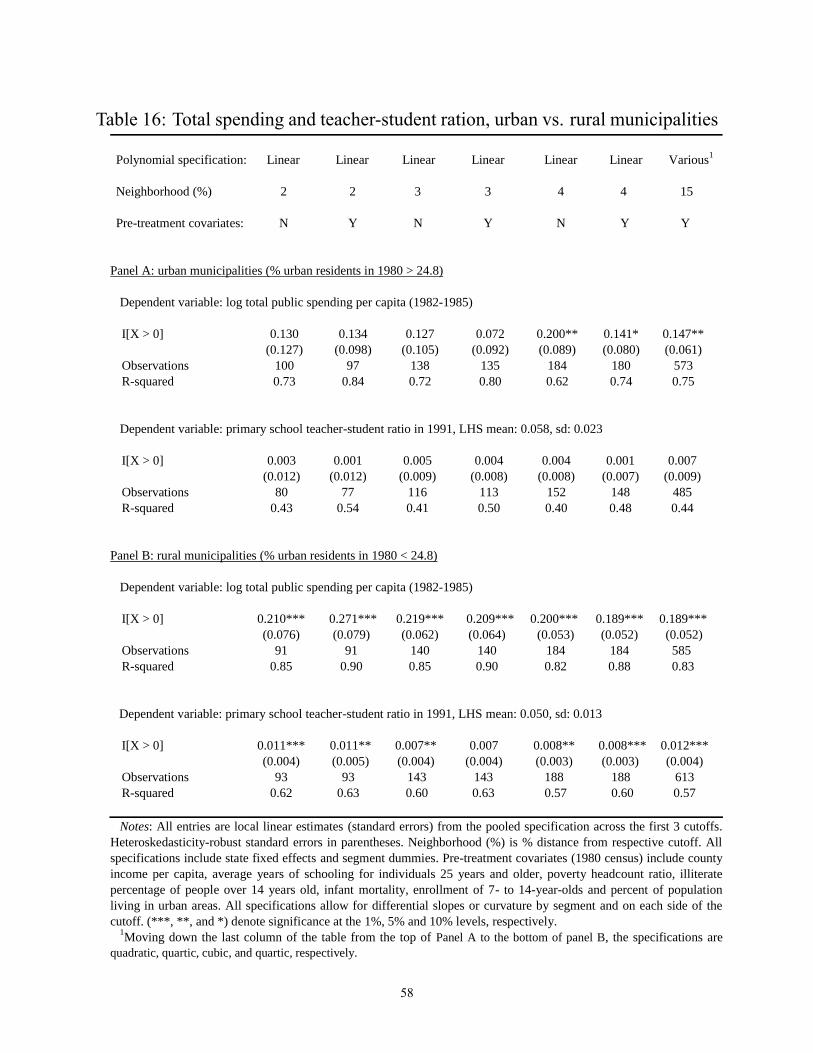
Table 16: Total spending and teacher-student ration, urban vs. rural municipalities
Polynomial specification: Linear Linear Linear Linear Linear Linear Various1
Neighborhood (%) 2 2 3 3 4 4 15
Pretreatment covariates: N Y N Y N Y Y
Panel A: urban municipalities (% urban residents in 1980 > 24.8)
Dependent variable: log total public spending per capita (19821985)
I[X > 0] 0.130 0.134 0.127 0.072 0.200** 0.141* 0.147**(0.127) (0.098) (0.105) (0.092) (0.089) (0.080) (0.061)
Observations 100 97 138 135 184 180 573Rsquared 0.73 0.84 0.72 0.80 0.62 0.74 0.75
Dependent variable: primary school teacherstudent ratio in 1991, LHS mean: 0.058, sd: 0.023
I[X > 0] 0.003 0.001 0.005 0.004 0.004 0.001 0.007(0.012) (0.012) (0.009) (0.008) (0.008) (0.007) (0.009)
Observations 80 77 116 113 152 148 485Rsquared 0.43 0.54 0.41 0.50 0.40 0.48 0.44
Panel B: rural municipalities (% urban residents in 1980 < 24.8)
Dependent variable: log total public spending per capita (19821985)
I[X > 0] 0.210*** 0.271*** 0.219*** 0.209*** 0.200*** 0.189*** 0.189***(0.076) (0.079) (0.062) (0.064) (0.053) (0.052) (0.052)
Observations 91 91 140 140 184 184 585Rsquared 0.85 0.90 0.85 0.90 0.82 0.88 0.83
Dependent variable: primary school teacherstudent ratio in 1991, LHS mean: 0.050, sd: 0.013
I[X > 0] 0.011*** 0.011** 0.007** 0.007 0.008** 0.008*** 0.012***(0.004) (0.005) (0.004) (0.004) (0.003) (0.003) (0.004)
Observations 93 93 143 143 188 188 613Rsquared 0.62 0.63 0.60 0.63 0.57 0.60 0.57
Notes: All entries are local linear estimates (standard errors) from the pooled specification across the first 3 cutoffs.Heteroskedasticityrobust standard errors in parentheses. Neighborhood (%) is % distance from respective cutoff. Allspecifications include state fixed effects and segment dummies. Pretreatment covariates (1980 census) include countyincome per capita, average years of schooling for individuals 25 years and older, poverty headcount ratio, illiteratepercentage of people over 14 years old, infant mortality, enrollment of 7 to 14yearolds and percent of populationliving in urban areas. All specifications allow for differential slopes or curvature by segment and on each side of thecutoff. (***, **, and *) denote significance at the 1%, 5% and 10% levels, respectively.
1Moving down the last column of the table from the top of Panel A to the bottom of panel B, the specifications arequadratic, quartic, cubic, and quartic, respectively.
58

Table 17: Schooling, literacy, poverty, urban vs. rural municipalities
Polynomial specification: Linear Linear Linear Linear Linear Linear Quartic
Neighborhood (%): 2 2 3 3 4 4 15
Pretreatment covariates: N Y N Y N Y Y
Panel A: urban municipalities (% urban residents in 1980 > 24.8)
Dependent variable: average years of schooling,19 to 28yearolds in 1991, LHS mean: 5.1, sd: 1.18
I[X > 0] 0.114 0.122 0.404 0.185 0.489** 0.163 0.128(0.316) (0.183) (0.266) (0.156) (0.223) (0.139) (0.167)
Observations 105 102 146 143 193 189 609Rsquared 0.68 0.88 0.71 0.87 0.69 0.86 0.86
Dependent variable: literacy rate, 19 to 28yearolds in 1991, LHS mean: 0.84, sd: 0.14
I[X > 0] 0.038* 0.038** 0.054*** 0.042*** 0.070*** 0.043*** 0.038***(0.022) (0.014) (0.019) (0.012) (0.017) (0.012) (0.013)
Observations 105 102 146 143 193 189 609Rsquared 0.87 0.94 0.87 0.94 0.85 0.93 0.91
Dependent variable: 1991 poverty rate, LHS mean: 0.52, sd: 0.22
I[X > 0] 0.051 0.057** 0.066* 0.045** 0.072** 0.038** 0.030***(0.044) (0.028) (0.034) (0.022) (0.031) (0.019) (0.001)
Observations 105 102 146 143 193 189 609Rsquared 0.82 0.95 0.84 0.94 0.82 0.93 0.92
Panel B: Rural Municipalities (% urban residents in 1980 < 24.8)
Dependent variable: average years of schooling, 19 to 28yearolds old in 1991, LHS mean: 3.5, sd: 1.38
I[X > 0] 0.351 0.237 0.589** 0.476 0.653*** 0.494*** 0.463**(0.412) (0.276) (0.297) (0.203) (0.243) (0.167) (0.211)
Observations 95 95 147 147 193 193 634Rsquared 0.72 0.89 0.75 0.88 0.73 0.87 0.87
Dependent variable: literacy rate, 19 to 28yearolds in 1991, LHS mean: 0.69, sd: 0.17
I[X > 0] 0.057 0.037 0.055 0.050* 0.056* 0.044** 0.043*(0.054) (0.038) (0.036) (0.027) (0.028) (0.022) (0.023)
Observations 95 95 147 147 193 193 634 Rsquared 0.72 0.91 0.78 0.91 0.78 0.90 0.88
Dependent variable: 1991 poverty rate, LHS mean: 0.76, sd: 0.15
I[X > 0] 0.002 0.041 0.048 0.050* 0.047 0.036 0.050*(0.045) (0.031) (0.034) (0.028) (0.029) (0.022) (0.026)
Observations 95 95 147 147 193 193 634Rsquared 0.77 0.88 0.73 0.87 0.71 0.85 0.85
Notes: All entries are local linear estimates (standard errors) from the pooled specification across the first 3 cutoffs.Heteroskedasticityrobust standard errors in parentheses. Neighborhood (%) is % distance from respective cutoff. Allspecifications include state fixed effects and segment dummies. Pretreatment covariates (1980 census) include countyincome per capita, average years of schooling for individuals 25 years and older, poverty headcount ratio, illiteratepercentage of people over 14 years old, infant mortality, enrollment of 7 to 14yearolds and percent of population livingin urban areas. All specifications allow for differential slopes or curvature by segment and on each side of the cutoff. (***,**, and *) denote significance at the 1%, 5% and 10% levels, respectively.
59

Figure1:FPMTransfers,1982-1985(in'000of2008Reais)
39786616925411915
1018
813
584
1698
023
772
3056
437
356
4414
819
82 o
ffic
ial p
opul
atio
nN
otes
: Eac
h do
t rep
rese
nts a
mun
icip
ality
. FPM
tran
sfer
s are
self
repo
rted
by m
unic
ipal
ities
. 198
2 of
ficia
lpo
pula
tion
is b
ased
on
the
1980
cen
sus c
ondu
cted
by
the
natio
nal s
tatis
tical
age
ncy,
IBG
E.
60

Figure2:EstimationApproach
c 1(1
p)
c1
c 1(1
+p)c
2(1p
) c
2c 2
(1+p
) c3(1
p)
c3
c 3(1
+p)
1982
off
icia
l pop
ulat
ion
(pop
)
Outcome variable (Y)
} τ1
} τ2
} τ3
61

Figure3:Histogramfor1982of�cialpopulation,smalltomediummunicipalities
020406080Frequency
1018
816
980
2377
230
564
3735
644
148
1982
off
icia
l pop
ulat
ion
Note
s: T
he b
inw
idth
is 2
83. 1
982
offic
ial p
opul
atio
n is
bas
ed o
n th
e 19
80 c
ensu
s co
nduc
ted
by th
e na
tiona
lsta
tistic
al a
genc
y, IB
GE.
McC
rary
den
sity
test
fails
to re
ject
the
null
of n
o di
scon
tinui
ty in
the
dens
ity a
tco
nven
tiona
l lev
els o
f sig
nific
ance
for t
he fi
rst s
ix c
utof
fs.
62

Figure4:Firststageandimpactsontotalrevenue,otherrevenueandownrevenue
.3.2.10.1.2.3 10%
8%
6%
4%
2%
02%
4%6%
8%10
%(P
opul
atio
nc)
/c
Pane
l A: l
og F
PM tr
ansf
ers p
er c
apita
.3.2.10.1.2.3 10%
8%
6%
4%
2%
02%
4%6%
8%10
%(P
opul
atio
nc)
/c
Pane
l B: l
og to
tal r
even
ue p
er c
apita
.3.2.10.1.2.3 10%
8%
6%
4%
2%
02%
4%6%
8%10
%(P
opul
atio
nc)
/c
Pane
l C: l
og o
ther
reve
nue
per c
apita
.3.2.10.1.2.3 10%
8%
6%
4%
2%
02%
4%6%
8%10
%(P
opul
atio
nc)
/c
Pane
l D: l
og o
wn
reve
nue
per c
apita
Not
es: A
ll va
riabl
es a
re s
umm
ed o
ver t
he p
erio
d 19
821
985
and
scal
ed b
y 19
80 m
unic
ipal
ity c
ensu
s pop
ulat
ion.
Eac
h do
tre
pres
ents
the
sam
ple
aver
age
of th
e (p
artia
lled
out)
depe
nden
t var
iabl
e in
a g
iven
bin
. The
bin
wid
th is
1 p
erce
ntag
e po
int
of th
e re
spec
tive
thre
shol
d, c
=10'
188,
13'58
4,16
'980
.
63

Figure5:Impactsontotalspendingandmainspendingcategories
.3.2.10.1.2.3 10%
8%
6%
4%
2%
02%
4%6%
8%10
%(P
opul
atio
nc)
/c
Pane
l A: l
og to
tal s
pend
ing
per c
apita
.3.2.10.1.2.3 10%
8%
6%
4%
2%
02%
4%6%
8%10
%(P
opul
atio
nc)
/c
Pane
l B: l
og e
duca
tion
spen
ding
per
cap
ita.3.2.10.1.2.3 1
0%8
%6
%4
%2
%0
2%4%
6%8%
10%
(Pop
ulat
ion
c)/c
Pane
l C: l
og h
ousin
g sp
endi
ng p
er c
apita
.3.2.10.1.2.3 10%
8%
6%
4%
2%
02%
4%6%
8%10
%(P
opul
atio
nc)
/c
Pane
l D: l
og tr
ansp
orta
tion
spen
ding
per
cap
ita
Note
s: T
otal
spen
ding
is su
mm
ed o
ver t
he p
erio
d 19
821
985.
The
spen
ding
cat
egor
ies a
re su
mm
ed o
ver t
he p
erio
d 19
821
983.
All
varia
bles
are
scal
ed b
y 19
80 m
unic
ipal
ity c
ensu
s pop
ulat
ion.
Eac
h do
t rep
rese
nts t
he sa
mpl
e av
erag
e of
the
(par
tialle
d ou
t)de
pend
ent v
aria
ble
in a
giv
en b
in. T
he b
inw
idth
is 1
per
cent
age
poin
t of t
he re
spec
tive
thre
shol
d, c
=10'1
88,1
3'584
,16'9
80.
64

Figure6:Impactsondirectpublicservicemeasures
.004.0020.002.004 10%
8%
6%
4%
2%
02%
4%6%
8%10
%(P
opul
atio
nc)
/c
Pane
l A: t
each
ers
tude
nt ra
tio
505 10%
8%
6%
4%
2%
02%
4%6%
8%10
%(P
opul
atio
nc)
/c
Pane
l B: n
umbe
r of e
lem
enta
ry sc
hool
s505 1
0%8
%6
%4
%2
%0
2%4%
6%8%
10%
(Pop
ulat
ion
c)/c
Pane
l C: a
cces
s to
wat
er (%
)
42024 10%
8%
6%
4%
2%
02%
4%6%
8%10
%(P
opul
atio
nc)
/c
Pane
l D: a
cces
s to
elec
trici
ty (%
)
Not
es: E
ach
dot r
epre
sent
s the
sam
ple
aver
age
of th
e (p
artia
lled
out)
depe
nden
t var
iabl
e in
a g
iven
bin
. The
bin
wid
this
1 p
erce
ntag
e po
int o
f the
resp
ectiv
e th
resh
old,
c=1
0'188
,13'
584,
16'9
80.
65

Figure7:Impactsonschooling,literacyandhouseholdincome
3.64.24.85.4 10%
8%
6%
4%
2%
02%
4%6%
8%10
%(P
opul
atio
nc)
/c
Pane
l A: s
choo
ling,
19
to 2
8ye
aro
lds
.69.75.81.87 10%
8%
6%
4%
2%
02%
4%6%
8%10
%(P
opul
atio
nc)
/c
Pane
l B: l
itera
cy ra
te, 1
9 to
28
year
old
s.50.57.64.71 1
0%8
%6
%4
%2
%0
2%4%
6%8%
10%
(Pop
ulat
ion
c)/c
Pane
l C: p
over
ty ra
te
160200240280 10%
8%
6%
4%
2%
02%
4%6%
8%10
%(P
opul
atio
nc)
/c
Pane
l D: i
ncom
e pe
r cap
ita
Not
es: A
ll va
riabl
es b
ased
on
the
1991
cen
sus.
Eac
h do
t rep
rese
nts t
he s
ampl
e av
erag
e of
the
depe
nden
t var
iabl
e in
agi
ven
bin.
The
bin
wid
th is
1 p
erce
ntag
e po
int o
f the
resp
ectiv
e th
resh
old,
c=1
0'18
8,13
'584
,16'9
80.
66
Recommended