Financial Constraints, Asset Tangibility, andCorporate

Investment*

Heitor Almeida

New York University and NBER

Murillo Campello

University of Illinois and NBER

(This version: September 17, 2006)

*Corresponding author: Murillo Campello, Wohlers Hall 430-A, 1206 South Sixth Street, Champaign, IL

61820. E-mail: campello@uiuc.edu. We thank Matias Braun, Charlie Calomiris, Glenn Hubbard (NBER

discussant), Owen Lamont, Anthony Lynch, Bob McDonald (the editor), Eli Ofek, Leonardo Rezende, David

Scharfstein, Rodrigo Soares, Sheri Tice, Greg Udell, Belén Villalonga (AFA discussant), Daniel Wolfenzon,

and an anonymous referee for their suggestions. Comments from seminar participants at the AFA meetings

(2005), Baruch College, FGV-Rio, Indiana University, NBER Summer Institute (2003), New York University,

and Yale University are also appreciated. Joongho Han provided support with GAUSS programming. Patrick

Kelly and Sherlyn Lim assisted us with the Census data collection. All remaining errors are our own.

1

© The Author 2007. Published by Oxford University Press on behalf of The Society for Financial Studies.All rights reserved. For permissions, please email: journals.permissions@oxfordjournals.org.

RFS Advance Access published April 12, 2007

Abstract

Pledgeable assets support more borrowing, which allows for further investment in pledgeable

assets. We use this credit multiplier to identify the impact of �nancing frictions on corporate

investment. The multiplier suggests that investment�cash �ow sensitivities should be increasing

in the tangibility of �rms�assets (a proxy for pledgeability), but only if �rms are �nancially

constrained. Our empirical results con�rm this theoretical prediction. Our approach is not

subject to the Kaplan and Zingales (1997) critique, and sidesteps problems stemming from

unobservable variation in investment opportunities. Thus, our results strongly suggest that

�nancing frictions a¤ect investment decisions.

2

Whether �nancing frictions in�uence real investment decisions is an important matter in con-

temporary �nance. Unfortunately, identifying �nancing�investment interactions is not an easy task.

The standard identi�cation strategy is based on the work of Fazzari et al. (1988), who argue that

the sensitivity of investment to internal funds should increase with the wedge between the costs of

internal and external funds (monotonicity hypothesis).1 Accordingly, one should be able to gauge

the impact of credit frictions on corporate spending by comparing the sensitivity of investment to

cash �ow across samples of �rms sorted on proxies for �nancing constraints. A number of recent

papers, however, question this approach. Kaplan and Zingales (1997) argue that the monotonic-

ity hypothesis is not a necessary property of optimal constrained investment, and report evidence

that contradicts Fazzari et al.�s �ndings. Erickson and Whited (2000), Gomes (2001), and Alti

(2003) further show that the results reported by Fazzari et al. are consistent with models in which

�nancing is frictionless.

In this paper, we develop a new theoretical argument to identify whether �nancing frictions

a¤ect corporate investment. We explore the idea that variables that increase a �rm�s ability to

obtain external �nancing may also increase investment when �rms have imperfect access to credit.

One such variable is the tangibility of a �rm�s assets. Assets that are more tangible sustain more

external �nancing because such assets mitigate contractibility problems: tangibility increases the

value that can be captured by creditors in default states. Building on Kiyotaki and Moore�s (1997)

credit multiplier, we show that investment�cash �ow sensitivities are increasing in the tangibility

of constrained �rms� assets. However, we �nd that tangibility has no e¤ect on the cash �ow

sensitivities of �nancially unconstrained �rms. Crucially, asset tangibility itself a¤ects the credit

status of the �rm, as �rms with very tangible assets may become unconstrained. This argument

implies a non-monotonic e¤ect of tangibility on cash �ow sensitivities: at low levels of tangibility,

the sensitivity of investment to cash �ow increases with asset tangibility, but this e¤ect disappears

3

at high levels of tangibility.

We use our theory to formulate an empirical test of the interplay between �nancial constraints

and investment based on a di¤erences-in-di¤erences approach. Using a sample of manufacturing

�rms drawn from COMPUSTAT between 1985 and 2000, we compare the e¤ect of tangibility on

investment�cash �ow sensitivities across di¤erent regimes of �nancial constraints. Our investment

equations resemble those of Fazzari et al., but include an interaction term that captures the e¤ect of

asset tangibility on investment�cash �ow sensitivities. We consider various measures of tangibility.

Our baseline proxy is taken from Berger et al. (1996) and gauges the expected liquidation value of

�rms�main categories of operating assets (cash, accounts receivable, inventories, and �xed capital).

Additional (industry-level) proxies gauge the salability of second-hand assets (cf. Shleifer and

Vishny (1992)). As is standard, our investment equations are separately estimated across samples

of constrained and unconstrained �rms. However, our benchmark tests do not rely on a priori

assignments of �rms into �nancial constraint categories. Instead, we employ a switching regression

framework in which the probability that �rms face constrained access to credit is jointly estimated

with the investment equations. In line with our theory, we include tangibility as a determinant of the

�rm�s constraint status, alongside other variables suggested by previous research (e.g., Hovakimian

and Titman (2004)).2

Our tests show that asset tangibility positively a¤ects the cash �ow sensitivity of investment in

�nancially constrained �rms, but not in unconstrained �rms. The results are identical whether we

use maximum likelihood (switching regression), traditional OLS, or error-consistent GMM estima-

tors, and our inferences are the same whether we use �rm- or industry-level proxies for tangibility.

The impact of asset tangibility on constrained �rms�investment is economically signi�cant. Finally,

the switching regression estimator suggests that �rms with higher tangibility are more likely to be

�nancially unconstrained. These �ndings are strongly consistent with our hypotheses.

4

Our approach mitigates the criticisms of the Fazzari et al. methodology. First, our approach

is not subject to the Kaplan and Zingales�critique. In fact, our identi�cation strategy explicitly

incorporates their argument that investment�cash �ow sensitivities are not monotonically related

to the degree of �nancing constraints. In contrast to Kaplan and Zingales, however, we argue

that investment�cash �ow sensitivities can be used to gauge the e¤ect of �nancing frictions on

investment. Second, our approach sidesteps the impact of biases stemming from unobservable

variation in investment opportunities. Unlike standard Fazzari et al. results, our �ndings cannot

be easily reconciled with models in which �nancing is frictionless.

Our study is not the �rst attempt at addressing the problems in Fazzari et al. Whited (1992)

and Hubbard et al. (1995) adopt an Euler equation approach to test for �nancial constraints. As

discussed by Gilchrist and Himmelberg (1995), however, this approach is unable to identify con-

straints when �rms are as constrained today as they are in the future. Blanchard et al. (1994),

Lamont (1997), and Rauh (2006) use �natural experiments� to bypass the need to control for

investment opportunities. However, it is di¢ cult to generalize �ndings derived from natural ex-

periments to other settings (see Rosenzweig and Wolpin (2000)). Almeida et al. (2004) use the

cash �ow sensitivity of cash holdings to test for �nancial constraints. While they only examine

a �nancial variable, this study establishes a link between �nancing frictions and real corporate

decisions. Overall, our paper provides a unique complement to the literature, suggesting new ways

in which to study the impact of �nancial constraints on �rm behavior.

The paper is organized as follows: Section 1 formalizes our hypotheses about the relation

between investment�cash �ow sensitivities, asset tangibility, and �nancial constraints; Section 2

uses our proposed strategy to test for �nancial constraints in a large sample of �rms; and Section

3 concludes.

5

1 The Model

To identify the e¤ect of tangibility on investment we study a simple theoretical framework in which

�rms have limited ability to pledge cash �ows from new investments. We use Hart and Moore�s

(1994) inalienability of human capital assumption to justify limited pledgeability, since this allows

us to derive our main implications in a simple, intuitive way. As we discuss in Section 1.2.1,

however, our results do not hinge on the inalienability assumption.

1.1 Analysis

The economy has two dates, 0 and 1. At time 0, the �rm has access to a production technology f(I)

that generates output (at time 1) from physical investment I. f(I) satis�es standard functional

assumptions, but production only occurs if the entrepreneur inputs her human capital. By this

we mean that if the entrepreneur abandons the project, only the physical investment I is left in

the �rm. We assume that some amount of external �nancing, B, may be needed to initiate the

project. Since human capital is inalienable, the entrepreneur cannot credibly commit her input to

the production process. It is common knowledge that she may renege on any contract she signs,

forcing renegotiation at a future date. As shown in Hart and Moore (1994), if creditors have no

bargaining power the contractual outcome in this framework is such that they will only lend up to

the expected value of the �rm in liquidation. This amount of credit can be sustained by a promised

payment equal to the value of physical investment goods under creditors�control and a covenant

establishing a transfer of ownership to creditors in states when the entrepreneur does not make the

payment.

Let the physical goods invested by the �rm have a price equal to 1, which is constant across

time. We model the pledgeability of the �rm�s assets by assuming that liquidation of those assets by

creditors entails �rm-speci�c transaction costs that are proportional to the value of the assets. More

6

precisely, if a �rm�s physical assets are seized by its creditors at time 1, only a fraction � 2 (0; 1)

of I can be recovered. � is a natural function of the tangibility of the �rm�s physical assets and

of other factors, such as the legal environment that dictates the relations between borrowers and

creditors.3 Firms with high � are able to borrow more because they invest in assets whose value

can be largely recaptured by creditors in liquidation states.

Creditors�valuation of assets in liquidation, �I, will establish the �rm�s borrowing constraint:

B � �I; (1)

where B is the amount of new debt that is supported by the project. Besides the new invest-

ment opportunity, we suppose that the �rm also has an amount W of internal funds available for

investment.

The entrepreneur maximizes the value of new investment I. Assuming that the discount rate

is equal to zero, the entrepreneur�s program can be written as:

maxI

f(I)� I, s:t: (2)

I �W + �I: (3)

The �rst-best level of investment, IFB, is such that f0(IFB) = 1. If the constraint in (3)

is satis�ed at IFB, the �rm is �nancially unconstrained. Thus, investment is constrained (i.e.,

I� < IFB) when

� < ��(W; IFB) = max

�1� W

IFB; 0

�: (4)

Notice that 0 � ��(W; IFB) � 1, and that if IFB �W < 0 the �rm is unconstrained irrespective of

the level of � (hence �� = 0). If the �rm is constrained, the level of investment is determined by

the �rm�s budget (or credit) constraint. The general expression for the optimal level of investment

7

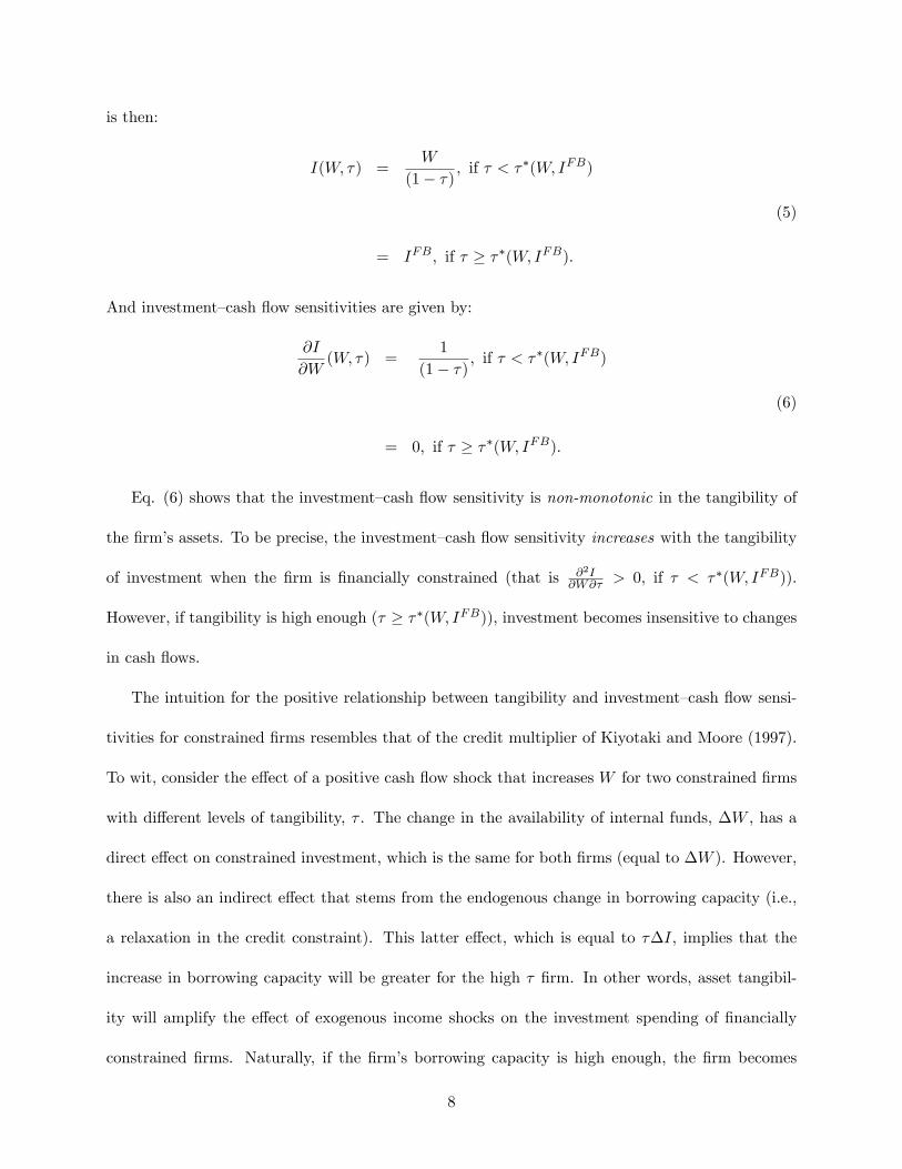
is then:

I(W; �) =W

(1� �) ; if � < ��(W; IFB)

(5)

= IFB; if � � ��(W; IFB):

And investment�cash �ow sensitivities are given by:

@I

@W(W; �) =

1

(1� �) ; if � < ��(W; IFB)

(6)

= 0; if � � ��(W; IFB):

Eq. (6) shows that the investment�cash �ow sensitivity is non-monotonic in the tangibility of

the �rm�s assets. To be precise, the investment�cash �ow sensitivity increases with the tangibility

of investment when the �rm is �nancially constrained (that is @2I@W@� > 0, if � < ��(W; IFB)).

However, if tangibility is high enough (� � ��(W; IFB)), investment becomes insensitive to changes

in cash �ows.

The intuition for the positive relationship between tangibility and investment�cash �ow sensi-

tivities for constrained �rms resembles that of the credit multiplier of Kiyotaki and Moore (1997).

To wit, consider the e¤ect of a positive cash �ow shock that increases W for two constrained �rms

with di¤erent levels of tangibility, � . The change in the availability of internal funds, �W , has a

direct e¤ect on constrained investment, which is the same for both �rms (equal to �W ). However,

there is also an indirect e¤ect that stems from the endogenous change in borrowing capacity (i.e.,

a relaxation in the credit constraint). This latter e¤ect, which is equal to ��I, implies that the

increase in borrowing capacity will be greater for the high � �rm. In other words, asset tangibil-

ity will amplify the e¤ect of exogenous income shocks on the investment spending of �nancially

constrained �rms. Naturally, if the �rm�s borrowing capacity is high enough, the �rm becomes

8

unconstrained and the investment�cash �ow sensitivity drops to zero. This implies that further

changes in tangibility will have no impact on the investment�cash �ow sensitivity of a �rm that

is �nancially unconstrained. We state these results in a proposition that motivates our empirical

strategy:

Proposition 1 The cash �ow sensitivity of investment, @I@W , bears the following relationship with

asset tangibility:

i) At low levels of tangibility (� < ��(W; IFB)), the �rm is �nancially constrained and

@I@W increases in asset tangibility,

ii) At high levels of tangibility (� � ��(W; IFB)), the �rm is �nancially unconstrained and

@I@W is independent of asset tangibility:

Whether the �rm is �nancially constrained depends not only on asset tangibility, but also on

other variables that a¤ect the likelihood that the �rm will be able to undertake all of its investment

opportunities. In the model, these variables are subsumed in the cut-o¤ ��(W; IFB). If �� is high,

the �rm is more likely to be �nancially constrained. The simple model we analyze suggests that ��

is increasing in the �rm�s investment opportunities (IFB), and decreasing in the �rm�s availability

of funds for investment (W ). More generally, however, �� should be a function of other variables

that a¤ect the �rm�s external �nancing premium. Accordingly, the empirical analysis considers

not only the variables used in the model above, but also other variables that prior literature has

identi�ed as being indicative of �nancing frictions.

1.2 Discussion

Before we move on to the empirical analysis, we discuss a few issues related to our theory.

9

1.2.1 Inalienability of human capital and creditor bargaining power

We used Hart and Moore�s (1994) inalienability of human capital assumption to derive our main

proposition. A natural question is: what elements of the Hart and Moore framework are strictly

necessary for our results to hold?

The crucial element of our theory is that the capacity for external �nance generated by new

investments is a positive function of the tangibility of the �rm�s assets (the credit multiplier). The

Hart and Moore (1994) setup is a convenient way to generate a relationship between debt capacity

and tangibility, but it is not the only way to get at the credit multiplier. Alternatively, one can argue

that asset tangibility reduces asymmetric information problems because tangible assets�payo¤s are

easier to observe. Bernanke et al. (1996) explore yet another rationale (namely, agency problems)

in their version of the credit multiplier. Finally, in an earlier version of the model we use Holmstrom

and Tirole�s (1997) theory of moral hazard in project choice to derive similar implications.

We also assumed that creditors have no bargaining power when renegotiating debt repayments

with entrepreneurs. In this way, speci�ed payments cannot exceed liquidation (collateral) values,

which is the creditor�s outside option. A similar link between collateral values and debt capacity

is assumed in the related papers of Kiyotaki and Moore (1997) and Diamond and Rajan (2001),

who in addition show that the link between debt capacity and collateral does not go away when

creditors have positive bargaining power.

1.2.2 Quantity versus cost constraints

In Section 1.1 we assumed a quantity constraint on external funds: �rms can raise external �nance

up to the value of collateralized debt, and they cannot raise additional external funds irrespective

of how much they would be willing to pay. We note, however, that there will be a multiplier e¤ect

even if �rms can raise external �nance beyond the limit implied by the quantity constraint. The

10

key condition that is required for the multiplier to remain operative is that raising external funds

beyond this limit entails a deadweight cost of external �nance (in addition to the fair cost of raising

funds). A reasonable assumption supporting this story is that the marginal deadweight cost of

external funds is increasing in the amount of uncollateralized �nance that the �rm is raising (as in

Froot et al. (1993) and Kaplan and Zingales (1997)).

Under the deadweight cost condition, the relation between tangibility and the multiplier arises

from the simple observation that having more collateral reduces the cost premium associated with

external funds. If tangibility is high, a given increase in investment has a lower e¤ect on the marginal

cost of total (i.e., collateralized and uncollateralized) external �nance because it creates higher

collateralized debt capacity. If tangibility is low, on the other hand, then the cost of borrowing

increases very rapidly, as the �rm has to tap more expensive sources of �nance in order to fund

the new investment. Because increases in �nancing costs dampen the e¤ect of a cash �ow shock,

investment will tend to respond more to a cash �ow shock when the tangibility of the underlying

assets is high (a detailed derivation is available from the authors).

2 Empirical Tests

To implement a test of Proposition 1, we need to specify an empirical model relating investment

with cash �ows and asset pledgeability. We will tackle this issue shortly. First we describe our

data.

2.1 Data Selection

Our sample selection approach is roughly similar to that of Gilchrist and Himmelberg (1995), and

Almeida et al. (2004). We consider the universe of manufacturing �rms (SICs 2000�3999) over the

1985�2000 period with data available from COMPUSTAT�s P/S/T and Research tapes on total

11

assets, market capitalization, capital expenditures, cash �ow, and plant property and equipment

(capital stock). We eliminate �rm-years for which the value of capital stock is less than $5 million,

those displaying real asset or sales growth exceeding 100%, and those with negative Q or with

Q in excess of 10. The �rst selection rule eliminates very small �rms from the sample, those for

which linear investment models are likely inadequate (see Gilchrist and Himmelberg). The second

rule eliminates those �rm-years registering large jumps in business fundamentals (size and sales);

these are typically indicative of mergers, reorganizations, and other major corporate events. The

third data cut-o¤ is introduced as a �rst, crude attempt to address problems in the measurement

of investment opportunities in the raw data and in order to improve the �tness of our investment

demand model � Abel and Eberly (2001), among others, discuss the poor empirical �t of linear

investment equations at high levels of Q.4 We de�ate all series to 1985 dollars using the CPI.

Many studies in the literature use relatively short data panels and require �rms to provide

observations during the entire period under investigation (e.g., Whited (1992), Himmelberg and

Petersen (1994), and Gilchrist and Himmelberg (1995)). While there are advantages to this attrition

rule in terms of series consistency and stability of the data process, imposing it on our 16-year-long

sample would lead to obvious concerns with survivorship biases. We instead require that �rms only

enter our sample if they appear for at least three consecutive years in the data. This is the minimum

number of years required for �rms to enter our estimations given the lag structure of our regression

models and our instrumental-variables approach. Our sample consists of 18,304 �rm-years.

2.2 An Empirical Model of Investment, Cash Flow, and Asset Tangibility

2.2.1 Speci�cation

We experiment with a parsimonious model of investment demand, augmenting the traditional

investment equation with a proxy for asset tangibility and an interaction term that allows the e¤ect

12

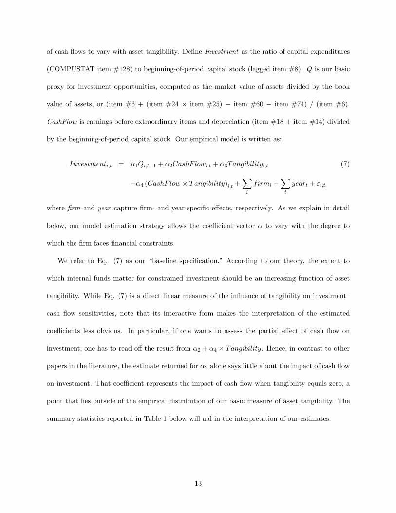
of cash �ows to vary with asset tangibility. De�ne Investment as the ratio of capital expenditures

(COMPUSTAT item #128) to beginning-of-period capital stock (lagged item #8). Q is our basic

proxy for investment opportunities, computed as the market value of assets divided by the book

value of assets, or (item #6 + (item #24 � item #25) � item #60 � item #74) / (item #6).

CashFlow is earnings before extraordinary items and depreciation (item #18 + item #14) divided

by the beginning-of-period capital stock. Our empirical model is written as:

Investmenti;t = �1Qi;t�1 + �2CashF lowi;t + �3Tangibilityi;t (7)

+�4 (CashF low � Tangibility)i;t +Xi

firmi +Xt

yeart + "i;t;

where �rm and year capture �rm- and year-speci�c e¤ects, respectively. As we explain in detail

below, our model estimation strategy allows the coe¢ cient vector � to vary with the degree to

which the �rm faces �nancial constraints.

We refer to Eq. (7) as our �baseline speci�cation.� According to our theory, the extent to

which internal funds matter for constrained investment should be an increasing function of asset

tangibility. While Eq. (7) is a direct linear measure of the in�uence of tangibility on investment�

cash �ow sensitivities, note that its interactive form makes the interpretation of the estimated

coe¢ cients less obvious. In particular, if one wants to assess the partial e¤ect of cash �ow on

investment, one has to read o¤ the result from �2 + �4 � Tangibility. Hence, in contrast to other

papers in the literature, the estimate returned for �2 alone says little about the impact of cash �ow

on investment. That coe¢ cient represents the impact of cash �ow when tangibility equals zero, a

point that lies outside of the empirical distribution of our basic measure of asset tangibility. The

summary statistics reported in Table 1 below will aid in the interpretation of our estimates.

13

2.2.2 Model Estimation

To test our theory, we need to identify �nancially constrained and unconstrained �rms. Following

the work of Fazzari et al. (1988), the standard approach in the literature is to use exogenous,

a priori sorting conditions that are hypothesized to be associated with the extent of �nancing

frictions that �rms face (see Erickson and Whited (2000), Almeida et al., (2004), and Hennessy

and Whited (2006) for recent examples of this strategy). After �rms are sorted into constrained

and unconstrained groups, Eq. (7) could be separately estimated across those di¤erent categories.

One of the central predictions of our theory, however, is that the �nancial constraint status

is endogenously related to the tangibility of the �rm�s assets. Hence, we need an estimator that

incorporates the e¤ect of tangibility both on cash �ow sensitivities and on the constraint status.

To allow for this e¤ect, we follow Hu and Schiantarelli (1998) and Hovakimian and Titman (2004)

and use a switching regression model with unknown sample separation to estimate our investment

regressions. This model allows the probability of being �nancially constrained to depend on asset

tangibility and on standard variables used in the literature (e.g., �rm size, age, and growth oppor-

tunities). As explained next, the model simultaneously estimates the equations that predict the

constraint status and the investment spending of constrained and unconstrained �rms.

Our analysis takes the switching regression model as the baseline estimation procedure. How-

ever, for ease of replicability, and to aid in the comparability of our results with those in the previous

literature, we also use the more traditional a priori constraint classi�cation approach to test our

story.5

The switching regression model (endogenous constraint selection) Hu and Schiantarelli

(1998) and Hovakimian and Titman (2004) provide a detailed description of the switching regression

estimator. Our approach follows theirs very closely, with the only di¤erence being the use of asset

14

tangibility as a predictor of �nancial constraints. Here we give a brief summary of the methodology.

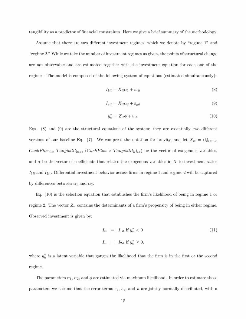
Assume that there are two di¤erent investment regimes, which we denote by �regime 1� and

�regime 2.�While we take the number of investment regimes as given, the points of structural change

are not observable and are estimated together with the investment equation for each one of the

regimes. The model is composed of the following system of equations (estimated simultaneously):

I1it = Xit�1 + "1it (8)

I2it = Xit�2 + "2it (9)

y�it = Zit�+ uit: (10)

Eqs. (8) and (9) are the structural equations of the system; they are essentially two di¤erent

versions of our baseline Eq. (7). We compress the notation for brevity, and let Xit = (Qi;t�1,

CashF lowi;t, Tangibilityi;t, (CashF low � Tangibility)i;t) be the vector of exogenous variables,

and � be the vector of coe¢ cients that relates the exogenous variables in X to investment ratios

I1it and I2it. Di¤erential investment behavior across �rms in regime 1 and regime 2 will be captured

by di¤erences between �1 and �2.

Eq. (10) is the selection equation that establishes the �rm�s likelihood of being in regime 1 or

regime 2. The vector Zit contains the determinants of a �rm�s propensity of being in either regime.

Observed investment is given by:

Iit = I1it if y�it < 0 (11)

Iit = I2it if y�it � 0;

where y�it is a latent variable that gauges the likelihood that the �rm is in the �rst or the second

regime.

The parameters �1, �2, and � are estimated via maximum likelihood. In order to estimate those

parameters we assume that the error terms "1 , "2 , and u are jointly normally distributed, with a

15

covariance matrix that allows for nonzero correlation between the shocks to investment and the

shocks to �rms�characteristics.6 The extent to which investment spending di¤ers across the two

regimes and the likelihood that �rms are assigned to either regime are simultaneously determined.

The approach yields separate regime-speci�c estimates for investment equations, dispensing with

the need to use ex-ante regime sortings.

We note that in order to fully identify the switching regression model we need to determine

which regime is the constrained one and which regime is the unconstrained. The algorithm speci�ed

in Eqs. (8)�(11) creates two groups of �rms that di¤er according to their investment behavior,

but it does not automatically tell the econometrician which �rms are constrained. To achieve

identi�cation, we need to use our theoretical priors about which �rm characteristics are associated

with �nancial constraints. As we will see below, this assignment turns out to be unambiguous in

our data.

One advantage of our approach is that it allows us to use multiple variables to predict whether

�rms are constrained or unconstrained in the selection equation (Eq. (10)). In contrast, the tradi-

tional method of splitting the sample according to a priori characteristics is typically implemented

using one characteristic at a time. In particular, the estimation of the selection equation allows us

to assess the statistical signi�cance of a given factor assumed to proxy for �nancing constraints,

while controlling for the information contained in other factors. Of course, one question is which

variables should be used in the selection vector Z. Here, we follow the existing literature but add

to the set of variables included in Z the main driver of our credit multiplier story: asset tangibility.

The set of selection variables that we consider comes directly from Hovakimian and Titman

(2004).7 Those variables naturally capture di¤erent ways in which �nancing frictions may be mani-

fested. The set includes a �rm�s size (proxied by the natural logarithm of total assets) and a �rm�s

age (proxied by the natural logarithm of the number of years the �rm appears in the COMPUSTAT

16

tapes since 1971). We label these variables LogBookAssets and LogAge, respectively. We construct

the other variables as follows. DummyDivPayout is a dummy variable that equals 1 if the �rm

has made any cash dividend payments in the year. ShortTermDebt is the ratio of short-term debt

(item #34) to total assets. LongTermDebt is the ratio of long-term debt (item #9) to total assets.

GrowthOpportunities is the ratio of market to book value of assets. DummyBondRating is a dummy

variable that equals 1 if the �rm has a bond rating assigned by Standard & Poors. FinancialSlack

is the ratio of cash and liquid securities to lagged assets. Finally, we include Tangibility in this set

(see de�nitions in Section 2.2.3). We enter all these variables in the selection equation in lagged

form.8

The standard regression model (ex-ante constraint selection) The standard empirical

approach uses ex-ante �nancial constraint sortings and least square regressions of investment equa-

tions. Estimations are performed separately for each constraint regime. We also use this approach

in our tests of the multiplier e¤ect, implementing the sorting schemes discussed in Almeida et al.

(2004):

� Scheme #1: In every year over the 1985�2000 period we rank �rms based on their payout

ratio and assign to the �nancially constrained (unconstrained) group those �rms in the bottom

(top) three deciles of the annual payout distribution. We compute the payout ratio as the ratio

of total distributions (dividends plus stock repurchases) to operating income. The intuition

that �nancially constrained �rms have signi�cantly lower payout ratios follows from Fazzari

et al. (1988).

� Scheme #2: In every year over the 1985�2000 period we rank �rms based on their total assets

and assign to the �nancially constrained (unconstrained) group those �rms in the bottom

(top) three deciles of the annual asset size distribution. This approach resembles Gilchrist

17

and Himmelberg (1995) and Erickson and Whited (2000), among others.

� Scheme #3: In every year over the 1985�2000 period we retrieve data on bond ratings assigned

by Standard & Poor�s and categorize those �rms with debt outstanding but without a bond

rating as �nancially constrained. Financially unconstrained �rms are those whose bonds are

rated. Similar approaches are used by, e.g., Kashyap et al. (1994), Gilchrist and Himmelberg

(1995), and Cummins et al. (1999).

� Scheme #4: In every year over the 1985�2000 period we retrieve data on commercial paper

ratings assigned by Standard & Poor�s and categorize those �rms with debt outstanding

but without a commercial paper rating as �nancially constrained. Financially unconstrained

�rms are those whose commercial papers are rated. This approach follows from the work of

Calomiris et al. (1995) on the characteristics of commercial paper issuers.

2.2.3 Tangibility measures

Asset tangibility (Tangibility) is measured in three alternative ways. First, we construct a �rm-level

measure of expected asset liquidation values that borrows from Berger et al. (1996). In determining

whether investors rationally value their �rms�abandonment option, Berger et al. gather data on

the proceeds from discontinued operations reported by a sample of COMPUSTAT �rms over the

1984�1993 period. The authors �nd that a dollar of book value yields, on average, 72 cents in exit

value for total receivables, 55 cents for inventory, and 54 cents for �xed assets. Following their

study, we estimate liquidation values for the �rm-years in our sample via the computation:

Tangibility = 0:715�Receivables+ 0:547� Inventory + 0:535� Capital;

where Receivables is COMPUSTAT item #2, Inventory is item #3, and Capital is item #8. As in

Berger et al., we add the value of cash holdings (item #1) to this measure and scale the result by

18

total book assets. Although we believe that the nature of the �rm production process will largely

determine the �rm�s asset allocation across �xed capital, inventories, etc., there could be some

degree of endogeneity in this measure of tangibility. In particular, one could argue that whether a

�rm is constrained might a¤ect its investments in more tangible assets and thus its credit capacity.

The argument for an endogenous bias in our tests along these lines, nonetheless, becomes a very

unlikely proposition when we use either one of the next two measures of tangibility.

The second measure of tangibility we use is a time-variant, industry-level proxy that gauges

the ease with which lenders can liquidate a �rm�s productive capital. Following Kessides (1990)

and Worthington (1995), we measure asset redeployability using the ratio of used to total (i.e.,

used plus new) �xed depreciable capital expenditures in an industry. The idea that the degree of

activity in asset resale markets � i.e., demand for second-hand capital � will in�uence �nancial

contractibility along the lines we explore here was �rst proposed by Shleifer and Vishny (1992).

To construct the intended measure, we hand-collect data for used and new capital acquisitions at

the four-digit SIC level from the Bureau of Census�Economic Census. These data are compiled

by the Bureau once every �ve years. We match our COMPUSTAT data set with the Census series

using the most timely information on the industry ratio of used to total capital expenditures for

every �rm-year throughout our sample period.9 Estimations based on this measure of tangibility

use smaller sample sizes since not all of COMPUSTAT�s SIC codes are covered by the Census and

recent Census surveys omit the new/used capital purchase breakdown.

The third measure of tangibility we consider is related to the proxy just discussed in that it

also gauges creditors�ability to readily dispose of a �rm�s assets. Based on the well-documented

high cyclicality of durable goods industry sales, we use a durable/nondurable industry dichotomy

that relates asset illiquidity to operations in the durables sector. This proxy is also in the spirit of

Shleifer and Vishny (1992), who emphasize the decline in collateralized borrowing in circumstances

19

in which assets in receivership will not be assigned to �rst-best alternative users: other �rms in the

same industry. To wit, because durable goods producers are highly cycle-sensitive, negative shocks

to demand will likely a¤ect all best alternative users of a durables producer�s assets, decreasing

tangibility. Our implementation follows the work of Sharpe (1994), who groups industries according

to the historical covariance between their sales and the GNP. The set of high covariance industries

includes all of the durable goods industries (except SICs 32 and 38) plus SIC 30. We refer to these

industries as �durables,�and label the remaining industries �nondurables.�We conjecture that the

assets of �rms operating in nondurables (durables) industries are perceived as more (less) liquid by

lenders, and assign to �rms in these industries the value of 1 (0).

Tangibility of new versus existing assets One potential caveat is that, strictly speaking,

Proposition 1 refers to variations in the tangibility of new investments. The three measures that we

use, however, refer to the tangibility of assets in place. If the assets that are acquired with the new

investment are of a similar nature to those that are already in place, then the distinction between

tangibility of new and existing assets is unimportant for most practical purposes. In this case, our

measures will be good proxies for the tangibility of new investment. We believe this is a reasonable

assumption for a very large portion of observed capital expenditures in our data, specially given

that we restrict our sample to manufacturing �rms, and discard from our sample those �rms that

display large jumps in business fundamentals (size and sales). These data �lters allow us to focus

on �rms whose demand for capital investment follows a more predictable/standard expansion path.

Unfortunately, data limitations preclude us from providing direct evidence for the conjecture

that the tangibility of assets in place is a good proxy for the tangibility of new investment. In

particular, we don�t have detailed information on the types of physical assets that are acquired

with the marginal dollar of investment. We note, however, that if the tangibility of the existing

20

assets is a poor proxy for the tangibility of marginal investments, then our tests should lack the

power to identify the credit multiplier e¤ect. In Section 2.6, we provide an indirect challenge to

our scale-enhancing assumption.

2.2.4 The use of Q in investment demand equations

One issue to consider is whether the presence of Q in our regressions will bias the inferences that

we can make about the impact of cash �ows on investment spending. Such concerns have become

a topic of debate in the literature, as evidence of higher investment�cash �ow sensitivities for

constrained �rms has been ascribed to measurement and interpretation problems with regressions

including Q (see Cummins et al. (1999), Erickson and Whited (2000), Gomes (2001), and Alti

(2003)). In particular, these papers have shown that the standard Fazzari et al. (1988) results

can be explained by models in which �nancing is frictionless, and in which Q is a noisy proxy for

investment opportunities.

Fortunately, these problems are unlikely to have �rst-order e¤ects on the types of inferences

about constrained investment that we can make with our tests. The standard argument in the

literature (e.g., Gomes (2001) and Alti (2003)) is that Q can be a comparatively poorer proxy for

investment opportunities for �rms typically classi�ed as �nancially constrained. This proxy quality

problem can bias upwards the level of investment�cash �ow sensitivities for �rms seen as constrained

even in the absence of �nancing frictions, because the cash �ow coe¢ cient captures information

about investment opportunities. Our proposed testing strategy sidesteps this problem because our

empirical test is independent of the level of the estimated cash �ow coe¢ cients of constrained and

unconstrained �rms. In contrast, it revolves around the marginal e¤ect of asset tangibility on the

impact of income shocks on spending under credit constraints. Even if the cash �ow coe¢ cient

contains information about investment opportunities, it is unlikely that the bias is higher both for

21

constrained and for highly tangible �rms. In particular, any bias that is systematically related to

the �nancial constraints proxies will be di¤erenced out by looking at the di¤erences between �rms

with highly tangible assets and those with less tangible assets.

Nevertheless, cross-sample di¤erences in the quality of the proxy for investment opportunities

are not the only source of problems for tests that rely on standard investment�cash �ow sensitivities.

In the context of the Fazzari et al. (1988) test, for example, Erickson and Whited (2000) have shown

that cross-sample di¤erences in the variance of cash �ows alone may generate di¤erences in cash

�ow sensitivities across constrained and unconstrained �rms when investment opportunities are

mismeasured. It is possible that similar statistical issues could bias the inferences that we can

make using the credit multiplier mechanism.10 We cannot completely rule out the possibility that

some property of the joint statistical distribution of the variables in our analysis, coupled with

measurement error, might introduce estimation biases that are di¢ cult to sign.

In order to provide more concrete evidence that mismeasurement in investment opportunities is

not explaining our results, we experiment with several techniques that produce reliable sensitivity

estimates even when such mismeasurement is important. First, we follow Cummins et al. (1999)

and estimate our baseline model using a GMM estimator that uses �nancial analysts� earnings

forecasts as instruments for Q. Second, we use the measurement error-consistent GMM estimator

suggested by Erickson and Whited (2000). Finally, we estimate Bond and Meghir�s (1994) Euler-

based empirical model of capital investment; this estimator entirely dispenses with the need to

include a Q in the set of regressors. As we will show, our main results hold under all these

estimation approaches.

22

2.3 Sample Characteristics

Our sample selection criteria and variable construction follow the standard in the �nancial con-

straints literature. The only exception concerns the central variable of our study: asset tangibility.

To save space, our discussion about basic sample characteristics revolves around that variable.

Table 1 reports detailed summary statistics for each of the three measures of asset tangibility we

use. The �rst tangibility measure indicates that a �rm�s assets in liquidation are expected to fetch,

on average, 53 cents on the dollar of book value. The second measure indicates that the average

industry-level ratio of used to total (i.e., used plus new) capital acquisitions is 7.4%. The third

indicates that 46.4% of the sample �rms operate in the nondurable goods industries.

Table 1 about here

Table 2 reports summary statistics for �rm investment, Q, and cash �ows, separately for �rms

with high and low tangibility levels. The purpose of this table is to check whether there are

distributional patterns in those three variables that are systematically related with asset tangibility.

Our �rst two measures of tangibility are continuous variables and we categorize as �low-tangibility�

(�high-tangibility�) �rms those �rms ranked in the bottom (top) three deciles of the tangibility

distribution; these rankings are performed on an annual basis. The third tangibility measure is

a dichotomous variable and we categorize as low-tangibility (high-tangibility) �rms those �rms in

durables (nondurables) industries. The numbers in Table 2 imply the absence of any systematic

patterns for investment demand, investment opportunities, and cash �ows across low- and high-

tangibility �rms. For example, while high-tangibility �rms seem to invest more and have higher

cash �ows according to the �rst two tangibility proxies, the opposite is true when the third proxy

is used.

Table 2 about here

23

2.4 Results

We �rst report and interpret the results from the switching regression model. Then we describe

the results we obtain when we use the standard estimation approach to investment spending across

constrained and unconstrained �rms.

2.4.1 Switching regressions

Table 3 presents the results returned from the switching regression estimation of our baseline

model (Eqs. (8)�(10)). Panel A contains the results from the structural investment equations

for constrained and unconstrained �rms. In this panel, each of the three rows reports the results

associated with a particular measure of asset tangibility. Panel B contains the results from the

constraint selection equations. In this panel, each of the three columns corresponds to a particular

measure of asset tangibility. In addition, the last row of panel B reports P -values for the test of the

null hypothesis that a single investment regime � as opposed to two regimes (constrained versus

unconstrained) � is su¢ cient to describe the data. This test is based on a likelihood ratio statistic,

for which the �2 distribution can be used for statistical inferences (cf. Goldfeld and Quandt (1976)).

We report a total of 6 investment equations (3 tangibility proxies � 2 constraints categories),

yielding 3 constrained�unconstrained comparison pairs. Since we use interaction terms in all of our

regressions and because the key variable used to gauge interaction e¤ects (namely, Tangibility) is

de�ned di¤erently across our estimations, we carefully discuss the economic meaning of all of the

estimates we report.

Table 3 about here

Consider the results from the selection equations (Panel B). As it turns out, the results we obtain

are very similar to those of Table 4 in Hovakimian and Titman (we note that the outputs from the

two papers have reversed signs by construction). As in their paper, we �nd that companies that

24

are smaller, that are younger, that pay lower amounts of dividends, that have greater investment

opportunities, that do not have bond ratings, and that carry greater �nancial slack are grouped

together into one of the investment regimes (regime 1).11 Our theoretical priors suggest that this

is the group of �rms that are most likely to be �nancially constrained. We also �nd that short-

and long-term ratios have relatively little e¤ect on the likelihood of being classi�ed in either group.

More important for our story, note that Tangibility leads to a lower probability of being in regime

1, that is, a lower probability of facing �nancial constraints � its implied e¤ect is comparable to

that of bond ratings.12 And this result is statistically signi�cant for each one of our tangibility

proxies.

Panel A of Table 3 reports the central �ndings of this paper. Based on the results from the

selection model, we call the �rms classi�ed in investment regime 1 (regime 2) �constrained�(�un-

constrained�) �rms. Notice that each and every one of the regression pairs in the table reveals

the same key result: constrained �rms� investment�cash �ow sensitivities are increasing in asset

tangibility, while unconstrained �rms�sensitivities show no or little response (often in the opposite

direction) to tangibility. Indeed, the interaction between cash �ow and tangibility attracts posi-

tive, statistically signi�cant coe¢ cients in all of the constrained �rm estimations. Further, these

coe¢ cients are uniformly higher than those of the unconstrained samples, and statistically di¤erent

at the 1% (alternatively, 5%) test level in all but one (alternatively, all) of the comparison pairs.

Because higher tangibility makes it more likely that a �rm will be unconstrained (Panel B), the

positive e¤ect of tangibility on investment�cash �ow sensitivities is most likely to obtain for low

levels of tangibility. These �ndings are fully consistent with the presence of a multiplier e¤ect for

constrained �rm investment that works along the lines of our model.

It is important to illustrate the impact of asset tangibility on the sensitivity of investment to cash

�ows when the �rm is �nancially constrained (the credit multiplier e¤ect). To do so, we consider

25

the estimates associated with our baseline measure of tangibility (�rst row of Panel A in Table 3).

Notice that when calculated at the �rst quartile of Tangibility (i.e., at 0:32, see Table 1), the partial

e¤ect of a one-standard-deviation cash �ow innovation (which is equal to 0:67) on investment per

dollar of capital is approximately 0:09. In contrast, at the third quartile of the same measure

(i.e., at 0:69), that partial e¤ect exceeds 0:20.13 To highlight the importance of these estimates we

note that the mean investment-to-capital ratio in our sample is 0:24. Analogous calculations for

unconstrained �rms yield mostly economically and statistically insigni�cant e¤ects regarding the

e¤ect of asset tangibility. Because we are not strictly estimating structural investment equations,

these economic magnitudes should be interpreted with some caution. Yet, they clearly ascribe an

important role to the credit multiplier in shaping the investment behavior of constrained �rms.

Notice that the coe¢ cients on CashFlow are negative in row 1 of Table 3, but positive in

the estimations reported in rows 2 and 3. The observed sign reversal is due to the impact of

the (tangibility-) �interaction� e¤ect on the �main� regression e¤ect of cash �ows, coupled with

the fact that Tangibility is a quite di¤erent regressor across the estimations in rows 1 through 3.

Importantly, the estimates in row 1 do not suggest that positive cash �ow shocks are detrimental to

�rm investment. To see this, note that although CashFlow attracts a negative coe¢ cient, in order

for cash �ow to hamper investment, Tangibility should equal zero (or be very close to zero), which

as one can infer from Table 1, is a point outside the empirical distribution of that �rm-level measure

of tangibility.14 Indeed, when we compute the partial e¤ect of cash �ows on investment we �nd that

these e¤ects are positive even at very low levels of tangibility. On the other hand, Tangibility is

often either very small or exactly zero when the industry-level measures of asset tangibility are used

in the estimations (rows 2 and 3). In those estimations, CashFlow returns a positive signi�cant

coe¢ cient, also consistent with the idea that cash �ow and investment are positively correlated,

even when tangibility is low.

26

The remaining estimates in Panel A of Table 3 display patterns that are also consistent with

our story and with previous research. For instance, the coe¢ cients returned for Q are in the same

range as those reported by Gilchrist and Himmelberg (1995) and Polk and Sapienza (2004), among

other comparable studies. Those coe¢ cients tend to be somewhat larger for the constrained �rms,

a pattern also seen in some of the estimations in Fazzari et al. (1988), Hoshi et al. (1991), and

Cummins et al. (1999). The coe¢ cients returned for Tangibility are positive in our estimations,

although statistically insigni�cant.

2.4.2 Standard regressions

Table 4 presents the results returned from the estimation of our baseline regression model for a

priori determined sample partitions and for each of our three tangibility proxies. Here, Eq. (7)

is estimated via OLS with �rm- and year-�xed e¤ects,15 and the error structure (estimated via

Huber-White) allows for residual heteroskedasticity and time clustering. We report a total of 8

estimated equations (4 constraints criteria � 2 constraints categories) in each of the 3 panels in the

table, yielding 12 constrained�unconstrained comparison pairs.

Table 4 about here

As in our previous estimations, notice that each one of the regression pairs in the table show

that constrained �rms�investment�cash �ow sensitivities are increasing in asset tangibility, while

unconstrained �rms�sensitivities show little or no response to tangibility. Once again, the inter-

action between cash �ow and tangibility attracts positive, statistically signi�cant coe¢ cients in all

of the constrained �rm estimations. And these coe¢ cients are uniformly higher than those of the

unconstrained samples: constrained�unconstrained coe¢ cient di¤erences are signi�cant at the 1%

test level in 10 of the 12 pairs. The results we obtain through this estimation approach are also

fully consistent with the presence of the credit multiplier e¤ect our theory describes. They are of

27

special interest in that they are very closely related to the types of tests implemented in the vast

literature on �nancial constraints.

2.5 Robustness

We subject our �ndings to a number of robustness checks in order to address potential concerns

with empirical biases in our estimations. These additional checks involve, among others, changes

to our baseline speci�cation (including the use of alternative lagging schemes), changes to proxy

construction and instrumentation, subsampling checks, and outlier treatment (e.g., winsorizing at

extreme quantiles). These tests produce no qualitative changes to our empirical �ndings and are

omitted from the paper for space considerations. In contrast, we report here a number of less

standard, more sophisticated checks of the reliability of our �ndings. These tests build on the

traditional constraint classi�cation approach, for which previous research has developed alternative

procedures meant to verify estimation robustness. It is worth pointing out that checks of the types

we describe below have been used to dismiss the inferences one achieves based on estimates of

investment�cash �ow sensitivities. We report the results from these checks in Table 5, where for

conciseness, we only present the estimates returned for the interaction term CashF low�Tangibility

� this term captures our credit multiplier e¤ect. For ease of exposition, we focus our discussion

on the results associated with our baseline proxy for asset tangibility.

The primary concern we want to address is the issue of measurement errors in our proxy for

investment opportunities, Q. We investigate the possibility that mismeasurement in investment

opportunities may a¤ect our inferences by using the estimators of three papers that tackle this

empirical issue: Cummins et al. (1999), Erickson and Whited (2000), and Bond and Meghir

(1994). Results from these GMM estimators (including the associated Hansen�s J -statistics for

28

overidenti�cation restrictions) are reported in Table 5.

Table 5 about here

In the �rst row of Table 5, we follow the work of Cummins et al. (1999) and use �nancial

analysts� forecasts of earnings as an instrument for Q in a GMM estimation of our investment

model. As in Almeida et al. (2004), we employ the median forecast of the two-year ahead earnings

scaled by lagged total assets to construct the earnings forecast measure. The set of instruments in

these estimations also includes lags 2 through 4 of �rm investment and cash �ows. Although only

some 80% of the �rm-years in our original sample provide valid observations for earnings forecasts,

our basic results remain.

The second row of Table 5 displays the interaction term coe¢ cients we obtain from the estima-

tor labeled GMM5 in Erickson and Whited (2000); this uses higher-order moment conditions for

identi�cation (as opposed to conditional mean restrictions).16 One di¢ culty we �nd in implement-

ing the estimator proposed by Erickson and Whited is isolating observations that are suitable for

their procedure. We can only isolate windows of three consecutive years of data after subjecting

our sample to those authors�data �pre-tests,� and these windows cover di¤erent stretches of our

sample period. Moreover, the use of their procedure fails to return estimates for the constraint

characterizations that are based on payout ratios and bond ratings.17 In spite of these limitations,

we �nd that our previous inferences continue to hold for each of the remaining constraint criteria.

In row 3, we experiment with the Euler-type investment model proposed by Bond and Meghir

(1994), by adding the lag of investment, its square, the lagged ratio of sales to capital, and the

squared, lagged debt-to-capital ratio to the set of regressors. In estimating this lagged dependent

variable model, we use the two-step dynamic panel GMM estimator proposed by Arellano and Bond

(1991), where di¤erenced regressors are instrumented by their lagged levels. A noticeable feature of

this empirical model is the absence of Q from the set of regressors � estimates are free from issues

29

concerning mismeasurement in Q. Results in row 3 show that our conclusions about the multiplier

e¤ect on constrained investment continue to hold.

The results in Table 5 suggest that biases stemming from unobservable variation in investment

opportunities cannot explain our main results. Unlike standard Fazzari et al. (1988) results, our

�ndings cannot be easily reconciled by models in which �nancing is frictionless.

2.6 Di¤erent Types of Investment: Fixed Capital versus R&D Expenditures

Our analysis has implicitly assumed that the tangibility of existing assets is a good proxy for

the tangibility of marginal investments (see Section 2.2.3). In this section, we revisit our proxy

assumption based on an indirect line of reasoning. To wit, we challenge our data assumptions

and experiment with the idea that if the tangibility of the existing assets is a poor proxy for the

tangibility of marginal investments, then our tests should lack the power to identify the credit

multiplier e¤ect.

To do so, we gather data on expenditures that do not obey the scale-enhancing restriction.

R&D expenditures constitute a good example. Irrespective of the tangibility of the �rm�s assets,

marginal R&D investments should be associated with very low tangibility (if any). Di¤erently from

capital expenditures, investments in intangible assets do not generate additional debt capacity, and

thus should not yield a multiplier e¤ect. Our theory would then suggest that we should not �nd

a credit multiplier e¤ect if we estimate the cash �ow sensitivity of R&D expenditures. While

con�rming this conjecture is not a direct proof that our scale-enhancing hypothesis is correct for

capital expenditures, it provides evidence that if our hypothesis were incorrect (i.e., that if we used

very poor proxies for marginal tangibility) we would not have found the results that we report.

To specify a test that isolates the multiplier e¤ect associated with R&D investments, we must

address the following complication. Because a cash �ow innovation will translate into variations

30

in both R&D and �xed capital expenditures for a constrained �rm (see Himmelberg and Petersen

(1994)), it is possible that the ampli�cation e¤ect that stems from regular capital expenditures will

correlate with spending in R&D. Hence, it is not necessarily the case that the cash �ow sensitivity

of R&D investment is uncorrelated with tangibility in the data, even when R&D adds nothing to

a �rm�s credit capacity.

This argument suggests that in order to isolate the R&D multiplier, we have to control for

the level of endogenous capital expenditures in the R&D regression. Because the e¤ect of (�xed

capital) tangibility on R&D is transmitted through a variation in capital expenditures, the cash

�ow sensitivity of R&D expenditures should then be independent of asset tangibility. One way

to perform this estimation is to use a two-stage least squares procedure, whereby we estimate the

�rm�s expected �xed investment in the �rst stage as a function of all of the exogenous parameters,

and then include the predicted values from this equation in a second-stage equation where we relate

R&D spending to cash �ows and endogenous �xed investment.

We implement this testing strategy by �tting our baseline investment equation (Eq. (7)) to

the data in order to generate predicted �xed capital investment values (denoted by bI) and thenestimating the following model:

IR&Di;t = �1bIi;t + �2CashF lowi;t + �3Tangibilityi;t (12)

+�4 (CashF low � Tangibility)i;t +Xi

firmi +Xt

yeart + "i;t:

Notice that we do not need to include proxies for investment opportunities in the set of regressors

in Eq. (12), because the e¤ect of investment opportunities is also subsumed in the relationship

between IR&D and bI. This insight in turn allows us to use lagged Q to identify the model.18 Our

hypothesis is that the e¤ect of cash �ow on R&D investment is independent of tangibility, even for

constrained �rms.

Table 6 reports the results from the estimation of Eq. (12) via switching regressions. Each

31

of the three rows in the table refers to one of our measures of tangibility, where we report the

results for the structural equations across constrained and unconstrained sample, but omit the

output from the selection equation. Focusing on the estimates of interest, note that while there

is indeed a strong association between R&D and �xed capital expenditures. Once we control for

this association, however, the sensitivity of R&D expenditures to cash �ow is not increasing in the

level of tangibility. In fact, all of the CashF low � Tangibility interaction terms attract negative

(mostly statistically insigni�cant) coe¢ cients. These results agree with our conjecture that the use

of poor proxies for marginal tangibility should lead to failure in uncovering the credit multiplier.

Table 6 about here

3 Concluding Remarks

Despite the theoretical plausibility of a channel linking �nancing frictions and real investment,

previous literature has found it di¢ cult to empirically identify this channel. This paper proposes

a novel identi�cation scheme, which is based on the e¤ect of asset pledgeability on �nancially

constrained corporate investment. Our strategy is not subject to the empirical problems that

have been associated with the traditional Fazzari et al.�s (1988) approach, since it does not rely

on a simple comparison of the levels of investment�cash �ow sensitivities across constrained and

unconstrained samples. Our approach also incorporates Kaplan and Zingales�s (1997) suggestion

that investment�cash �ow sensitivities need not decrease monotonically with variables that relax

�nancing constraints. We argue that this non-monotonicity can be used in a positive way, to help

uncover information about �nancing constraints that might be embedded in investment�cash �ow

sensitivities. We believe that our testing approach will prove useful for future researchers in need

of a reliable method of identifying the impact of �nancial constraints on investment and other

�nancial variables, and in more general contexts where investment�cash �ow sensitivities might

32

help in drawing inferences about the interplay between capital markets and corporate behavior.

The evidence we uncover in this paper is strongly consistent with a link between �nancing fric-

tions and investment. As we hypothesize, we �nd that while asset tangibility increases investment�

cash �ow sensitivities for �nancially constrained �rms, no such e¤ects are observed for unconstrained

�rms. Moreover, tangibility in�uences a �rm�s credit status according to theoretical expectations:

�rms with more tangible assets are less likely to be �nancially constrained. The positive e¤ect of

tangibility on constrained cash �ow sensitivities is evidence for a credit multiplier in U.S. corporate

investment. Income shocks have especially large e¤ects for constrained �rms with tangible assets,

because these �rms have highly procyclical debt capacity. This insight can have interesting impli-

cations for asset pricing and macroeconomics, which could be explored by future researchers and

policymakers.19

33

References

Abel, A., and J. Eberly, 2001, �Investment and Q with Fixed Costs: An Empirical Analysis,�Working paper, University of Pennsylvania.

Almeida, H., M. Campello, and C. Liu, 2006, �The Financial Accelerator: Evidence FromInternational Housing Markets,�Review of Finance 10, 1-32.

Almeida, H., M. Campello, and M. Weisbach, 2004, �The Cash Flow Sensitivity of Cash,�Journal of Finance 59, 1777-1804.

Alti, A., 2003, �How Sensitive is Investment to Cash Flow When Financing is Frictionless?�Journal of Finance 58, 707-722.

Arellano, M., and S. Bond, 1991, �Some Tests of Speci�cation for Panel Data: Monte CarloEvidence and an Application to Employment Equations,�Review of Economic Studies 58,277-297.

Berger, P., E. Ofek, and I. Swary, 1996, �Investor Valuation and Abandonment Option,�Journal of Financial Economics 42, 257-287.

Bernanke, B., M. Gertler, and S. Gilchrist, 1996, �The Financial Accelerator and the Flightto Quality,�Review of Economics and Statistics 78, 1-15.

Blanchard, O., F. Lopez-de-Silanes, and A. Shleifer, 1994, �What Do Firms Do with CashWindfalls?�Journal of Financial Economics 36, 337-360.

Bond, S., and C. Meghir, 1994, �Dynamic Investment Models and the Firm�s Financial Pol-icy,�Review of Economic Studies 61, 197-222.

Calomiris, C., C. Himmelberg, and P. Wachtel, 1995, �Commercial Paper and CorporateFinance: A Microeconomic Perspective,� Carnegie Rochester Conference Series on PublicPolicy 45, 203-250.

Calomiris, C., and R. G. Hubbard, 1995, �Internal Finance and Firm-Level Investment: Ev-idence from the Undistributed Pro�ts Tax of 1936-37,�Journal of Business 68, 443-482.

Cummins, J., K. Hasset, and S. Oliner, 1999, �Investment Behavior, Observable Expectations,and Internal Funds,�forthcoming, American Economic Review.

Devereux, M., and F. Schiantarelli, 1990, �Investment Financial Factors and Cash Flow: Ev-idence from UK Panel Data,�In: Hubbard, R. G. (Ed.), Asymmetric Information CorporateFinance and Investment, University of Chicago Press, Chicago, 279-306.

Diamond, D. and R. Rajan, 2001, �Liquidity Risk, Liquidity Creation, and Financial Fragility:A Theory of Banking,�Journal of Political Economy 109, 287-327.

Erickson, T., and T. Whited, 2000, �Measurement Error and the Relationship between In-vestment and Q,�Journal of Political Economy 108, 1027-1057.

Fazzari S., R. G. Hubbard, and B. Petersen, 1988, �Financing Constraints and CorporateInvestment,�Brookings Papers on Economic Activity 1, 141-195.

34

Fazzari, S., and B. Petersen, 1993, �Working Capital and Fixed Investment: New Evidenceon Financing Constraints,�RAND Journal of Economics 24, 328-342.

Froot, K., D. Scharfstein, and J. Stein, 1993, �Risk Management: Coordinating CorporateInvestment and Financing Policies,�Journal of Finance 48, 1629-1658.

Gan, J., 2006, �Financial Constraints and Corporate Investment: Evidence from an Exoge-nous Shock to Collateral,�forthcoming, Journal of Financial Economics.

Gilchrist, S., and C. Himmelberg, 1995, �Evidence on the Role of Cash Flow for Investment,�Journal of Monetary Economics 36, 541-572.

Goldfeld, S. and R. Quandt, 1976, �Techniques for Estimating Switching Regressions,� inGoldfeld and Quandt (eds.), Studies in Non-Linear Estimation, Cambridge: Ballinger, 3-36.

Gomes, J., 2001, �Financing Investment,�American Economic Review 91, 1263-1285.

Hahn, J. and H. Lee, 2005, �Financial Constraints, Debt Capacity, and the Cross Section ofStock Returns,�Working paper, University of Washington and Korea Development Institute.

Hart, O., and J. Moore, 1994, �A Theory of Debt Based on the Inalienability of HumanCapital,�Quarterly Journal of Economics 109, 841-879.

Hennessy, C., and T. Whited, 2006, �How Costly is External Financing? Evidence from aStructural Estimation,�forthcoming, Journal of Finance.

Himmelberg, C., and B. Petersen, 1994, �R&D and Internal Finance: A Panel Study of SmallFirms in High-Tech Industries,�Review of Economics and Statistics 76, 38-51.

Holmstrom, B., and J. Tirole, 1997, �Financial Intermediation, Loanable Funds and the RealSector,�Quarterly Journal of Economics 112, 663-691.

Hoshi, T., A. Kashyap, and D. Scharfstein, 1991, �Corporate Structure, Liquidity, and In-vestment: Evidence from Japanese Industrial Groups,�Quarterly Journal of Economics 106,33-60.

Hovakimian, G., and S. Titman, 2004, �Corporate Investment with Financial Constraints:Sensitivity of Investment to Funds from Voluntary Asset Sales,� forthcoming, Journal ofMoney, Credit, and Banking.

Hubbard, R. G., 1998, �Capital Market Imperfections and Investment,�Journal of EconomicLiterature 36, 193-227.

Hu, X., and F. Schiantarelli, 1997, �Investment and Capital Market Imperfections: A Switch-ing Regression Approach Using U.S. Firm Panel Data,�Review of Economics and Statistics79, 466-479.

Hubbard, R. G., Kashyap, A., andWhited, T., 1995, �Internal Finance and Firm Investment,�Journal of Money, Credit, and Banking 27, 683-701.

Kadapakkam, P., P. Kumar, and L. Riddick, 1998, �The Impact of Cash Flows and Firm Sizeon Investment: The International Evidence,�Journal of Banking and Finance 22, 293-320.

35

Kaplan, S., and L. Zingales, 1997, �Do Financing Constraints Explain why Investment isCorrelated with Cash Flow?�Quarterly Journal of Economics 112, 169-215.

Kashyap, A., O. Lamont, and J. Stein, 1994,�Credit Conditions and the Cyclical Behavior ofInventories,�Quarterly Journal of Economics 109, 565-592.

Kessides, I., 1990, �Market Concentration, Contestability, and Sunk Costs,�Review of Eco-nomics and Statistics 72, 614-622.

Kiyotaki, N., and J. Moore, 1997, �Credit Cycles,�Journal of Political Economy 105, 211-248.

Maddala, G. S., 1986, �Disequilibrium, Self-selection, and Switching Models,�in Griliches, Z.and M. D. Intriligator (eds.), Handbook of Econometrics, Vol.3, Amsterdam: Elsevier Science,1633-1688.

Myers, S., and R. Rajan, 1998, �The Paradox of Liquidity,�Quarterly Journal of Economics113, 733-777.

Polk, C., and P. Sapienza, 2004, �The Real E¤ects of Investor Sentiment,�Working paper,Northwestern University.

Rauh, J., 2006, �Investment and Financing Constraints: Evidence from the Funding of Cor-porate Pension Plans,�Journal of Finance 61, 33-71.

Rosenzweig, M., and K. Wolpin, 2000, �Natural �Natural Experiments�in Economics,�Jour-nal of Economic Literature 38, 827-874.

Sharpe, S., 1994, �Financial Market Imperfections, Firm Leverage and the Cyclicality ofEmployment,�American Economic Review 84, 1060-1074.

Shleifer, A., and R. Vishny, 1992, �Liquidation Values and Debt Capacity: A Market Equi-librium Approach,�Journal of Finance 47, 1343-1365.

Whited, T., 1992, �Debt, Liquidity Constraints, and Corporate Investment: Evidence fromPanel Data,�Journal of Finance 47, 425-460.

Worthington P., 1995, �Investment, Cash Flow, and Sunk Costs,�Journal of Industrial Eco-nomics 43, 49-61..

36

Endnotes

1. A partial list of papers that use this methodology includes Devereux and Schiantarelli (1990), Hoshi et

al. (1991), Fazzari and Petersen (1993), Himmelberg and Petersen (1994), Bond and Meghir (1994),

Calomiris and Hubbard (1995), Gilchrist and Himmelberg (1995), and Kadapakkam et al. (1998). See

Hubbard (1998) for a survey.

2. To allow for comparability with existing research, in complementary tests we assign observations into

groups of constrained and unconstrained �rms based only on characteristics such as payout policy,

size, and credit ratings.

3. Myers and Rajan (1998) parameterize the liquidity of a �rm�s assets in a similar way.

4. These same cut-o¤s for Q are used by Gilchrist and Himmelberg and we �nd that their adoption

reduces the average Q in our sample to about 1.0; only slightly lower than studies that use our same

data sources and de�nitions but that do not impose bounds on the empirical distribution of Q (Kaplan

and Zingales (1997) report an average Q of 1.2, while Polk and Sapienza (2004) report 1.6).

5. An advantage of using the traditional approach is that some of our robustness tests can only be

performed in this simpler setting, notably the use of measurement-error consistent GMM estimators

that we describe in Section 2.5.

6. The covariance matrix has the form =

26666664�11 �12 �1u

�21 �22 �2u

�u1 �u2 1

37777775, where var(u) is normalized to 1.See Maddala (1986), Hu and Schiantarelli (1998), and Hovakimian and Titman (2004) for additional

details.

7. The set of variables used in Hu and Schiantarelli (1997) resembles that of Hovakimian and Titman,

but is more parsimonious. We omit from the paper the results that we obtain with the use of this

37

alternative set. They are similar to what we report below.

8. In a previous version of the paper, we also used a second set of selection variables that closely resemble

those used in the ex-ante selection model below. The results are virtually identical to those reported

in Table 3 and are omitted for space considerations.

9. E.g., we use the 1987 Census to gauge the asset redeployability of COMPUSTAT �rms with �scal

years in the 1985�1989 window.

10. Taken literally, Erickson and Whited�s arguments imply that any regression featuring Q may be subject

to biases.

11. Note that the dependent variable in Panel B of Table 3 is a dummy that is equal to 1 if the �rm is in

investment regime 1, and 0 if the �rm is in investment regime 2.

12. For illustration, while holding other variables at their unconditional average values, a large (two

standard deviation) increase in Tangibility brings down the probability of being �nancially constrained

by about as much as the granting of a bond rating by S&P.

13. The partial e¤ects are equal to the standard deviation of cash �ows times the coe¢ cient on CashFlow,

plus that same standard deviation times the coe¢ cient on the interaction term times the level of

Tangibility (�rst or third quartiles).

14. The linear estimator for interactive models will produce vector coe¢ cients for the �main�e¤ects of the

interacted variables even when those e¤ects accrue to data points that lie outside of the actual sample

distribution. The minimum observation in the distribution of our baseline measure of tangibility is

0.11.

15. The only exception applies to the results in the last panel (durables/nondurables dichotomy), where

including �rm-�xed e¤ects is unfeasible since �rms are assigned to only one (time-invariant) industry

38

category.

16. We implement the GAUSS codes made available by Toni Whited in her Webpage.

17. Erickson and Whited, too, report these sampling di¢ culties in their paper; their sample is constrained

to a four-year window containing only 737 �rms. Di¤erently from their paper, our speci�cation features

a proxy for tangibility and a cash �ow�tangibility interaction term. This complicates our search for

a stretch of data that passes their estimator�s pre-tests. We could only �nd suitable samples of both

�nancially constrained and unconstrained �rms by size and commercial paper ratings over the 1996�

1998 and 1992�1994 periods, respectively.

18. We let Q provide the extra vector dimensionality necessary for model identi�cation because this follows

more naturally from the empirical framework we use throughout the paper. In unreported estimations,

however, we experiment with alternative regressors (e.g., sales growth) and obtain the same results.

19. See Hahn and Lee (2005) for recent evidence that the credit multiplier has implications for the cross-

section of stock returns, Almeida et al. (2006), for evidence that the credit multiplier ampli�es �uc-

tuations in housing prices and housing credit demand, and Gan (2006), who examines the interaction

between the credit multiplier and the collapse of Japanese land prices in the 1990�s.

39

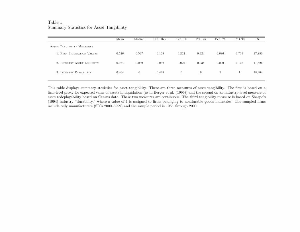
Table 1Summary Statistics for Asset Tangibility

Mean Median Std. Dev. Pct. 10 Pct. 25 Pct. 75 Pc.t 90 N

Asset Tangibility Measures

1. Firm Liquidation Values 0.526 0.537 0.169 0.262 0.324 0.686 0.739 17,880

2. Industry Asset Liquidity 0.074 0.059 0.052 0.026 0.038 0.099 0.136 11,826

3. Industry Durability 0.464 0 0.499 0 0 1 1 18,304

This table displays summary statistics for asset tangibility. There are three measures of asset tangibility. The �rst is based on a�rm-level proxy for expected value of assets in liquidation (as in Berger et al. (1996)) and the second on an industry-level measure ofasset redeployability based on Census data. These two measures are continuous. The third tangibility measure is based on Sharpe�s(1994) industry �durability,�where a value of 1 is assigned to �rms belonging to nondurable goods industries. The sampled �rmsinclude only manufacturers (SICs 2000�3999) and the sample period is 1985 through 2000.

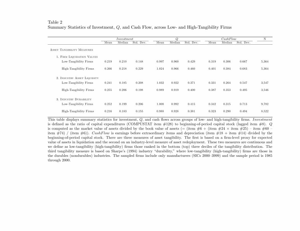
Table 2Summary Statistics of Investment, Q, and Cash Flow, across Low- and High-Tangibility Firms

Investment Q CashF low NMean Median Std. Dev. Mean Median Std. Dev. Mean Median Std. Dev.

Asset Tangibility Measures

1. Firm Liquidation Values

Low-Tangibility Firms 0.219 0.210 0.148 0.997 0.960 0.429 0.319 0.306 0.667 5,364

High-Tangibility Firms 0.266 0.218 0.229 1.024 0.966 0.460 0.401 0.384 0.683 5,364

2. Industry Asset Liquidity

Low-Tangibility Firms 0.241 0.185 0.208 1.032 0.922 0.371 0.331 0.264 0.547 3,547

High-Tangibility Firms 0.255 0.206 0.198 0.989 0.919 0.400 0.387 0.353 0.495 3,546

3. Industry Durability

Low-Tangibility Firms 0.252 0.199 0.206 1.008 0.992 0.415 0.342 0.315 0.713 9,782

High-Tangibility Firms 0.216 0.183 0.155 0.988 0.928 0.381 0.323 0.290 0.494 8,522

This table displays summary statistics for investment, Q, and cash �ows across groups of low- and high-tangibility �rms. Investmentis de�ned as the ratio of capital expenditures (COMPUSTAT item #128) to beginning-of-period capital stock (lagged item #8). Qis computed as the market value of assets divided by the book value of assets (= (item #6 + (item #24 � item #25) � item #60 �item #74) / (item #6)). CashF low is earnings before extraordinary items and depreciation (item #18 + item #14) divided by thebeginning-of-period capital stock. There are three measures of asset tangibility. The �rst is based on a �rm-level proxy for expectedvalue of assets in liquidation and the second on an industry-level measure of asset redeployment. These two measures are continuous andwe de�ne as low-tangibility (high-tangibility) �rms those ranked in the bottom (top) three deciles of the tangibility distribution. Thethird tangibility measure is based on Sharpe�s (1994) industry �durability,� where low-tangibility (high-tangibility) �rms are those inthe durables (nondurables) industries. The sampled �rms include only manufacturers (SICs 2000�3999) and the sample period is 1985through 2000.

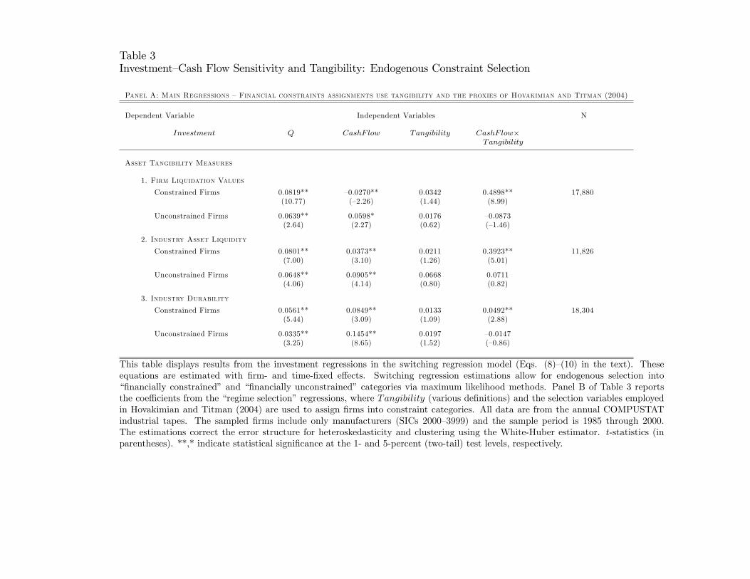
Table 3Investment�Cash Flow Sensitivity and Tangibility: Endogenous Constraint Selection

Panel A: Main Regressions �Financial constraints assignments use tangibility and the proxies of Hovakimian and Titman (2004)

Dependent Variable Independent Variables N

Investment Q CashF low Tangibility CashF low�Tangibility

Asset Tangibility Measures

1. Firm Liquidation Values

Constrained Firms 0.0819** �0.0270** 0.0342 0.4898** 17,880(10.77) (�2.26) (1.44) (8.99)

Unconstrained Firms 0.0639** 0.0598* 0.0176 �0.0873(2.64) (2.27) (0.62) (�1.46)

2. Industry Asset Liquidity

Constrained Firms 0.0801** 0.0373** 0.0211 0.3923** 11,826(7.00) (3.10) (1.26) (5.01)

Unconstrained Firms 0.0648** 0.0905** 0.0668 0.0711(4.06) (4.14) (0.80) (0.82)

3. Industry Durability

Constrained Firms 0.0561** 0.0849** 0.0133 0.0492** 18,304(5.44) (3.09) (1.09) (2.88)

Unconstrained Firms 0.0335** 0.1454** 0.0197 �0.0147(3.25) (8.65) (1.52) (�0.86)

This table displays results from the investment regressions in the switching regression model (Eqs. (8)�(10) in the text). Theseequations are estimated with �rm- and time-�xed e¤ects. Switching regression estimations allow for endogenous selection into��nancially constrained�and ��nancially unconstrained� categories via maximum likelihood methods. Panel B of Table 3 reportsthe coe¢ cients from the �regime selection�regressions, where Tangibility (various de�nitions) and the selection variables employedin Hovakimian and Titman (2004) are used to assign �rms into constraint categories. All data are from the annual COMPUSTATindustrial tapes. The sampled �rms include only manufacturers (SICs 2000�3999) and the sample period is 1985 through 2000.The estimations correct the error structure for heteroskedasticity and clustering using the White-Huber estimator. t-statistics (inparentheses). **,* indicate statistical signi�cance at the 1- and 5-percent (two-tail) test levels, respectively.

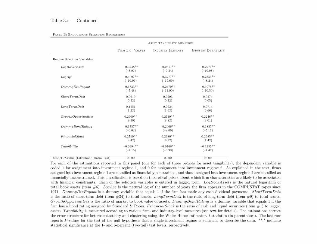
Table 3.: � Continued

Panel B: Endogenous Selection Regressions

Asset Tangibility Measures

Firm Liq. Values Industry Liquidity Industry Durability

Regime Selection Variables

LogBookAssets �0.3248** �0.2811** �0.2271**(�8.97) (�9.34) (�10.98)

LogAge �0.4097** �0.3277** �0.2355**(�10.96) (�15.69) (�8.24)

DummyDivPayout �0.1833** �0.2479** �0.1976**(�7.48) (�11.90) (�10.50)

ShortTermDebt 0.0919 0.0293 0.0274(0.22) (0.12) (0.05)

LongTermDebt 0.1551 0.0924 0.0714(1.22) (1.02) (0.66)

GrowthOpportunities 0.2609** 0.2719** 0.2246**(9.30) (8.82) (8.01)

DummyBondRating �0.1757** �0.2066** �0.1855**(�6.02) (�8.09) (�5.11)

FinancialSlack 0.2719** 0.2980** 0.2985**(8.42) (9.32) (7.42)

Tangibility �0.0994** �0.0766** �0.1255**(�7.15) (�6.98) (�7.42)

Model P -value (Likelihood Ratio Test) 0.000 0.000 0.000

For each of the estimations reported in this panel (one for each of three proxies for asset tangibility), the dependent variable iscoded 1 for assignment into investment regime 1, and 0 for assignment into investment regime 2. As explained in the text, �rmsassigned into investment regime 1 are classi�ed as �nancially constrained, and those assigned into investment regime 2 are classi�ed as�nancially unconstrained. This classi�cation is based on theoretical priors about which �rm characteristics are likely to be associatedwith �nancial constraints. Each of the selection variables is entered in lagged form. LogBookAssets is the natural logarithm oftotal book assets (item #6). LogAge is the natural log of the number of years the �rm appears in the COMPUSTAT tapes since1971. DummyDivPayout is a dummy variable that equals 1 if the �rm has made any cash dividend payments. ShortTermDebtis the ratio of short-term debt (item #34) to total assets. LongTermDebt is the ratio of long-term debt (item #9) to total assets.GrowthOpportunities is the ratio of market to book value of assets. DummyBondRating is a dummy variable that equals 1 if the�rm has a bond rating assigned by Standard & Poors. FinancialSlack is the ratio of cash and liquid securities (item #1) to laggedassets. Tangibility is measured according to various �rm- and industry-level measures (see text for details). The estimations correctthe error structure for heteroskedasticity and clustering using the White-Huber estimator. t-statistics (in parentheses). The last rowreports P -values for the test of the null hypothesis that a single investment regime is su¢ cient to describe the data. **,* indicatestatistical signi�cance at the 1- and 5-percent (two-tail) test levels, respectively.

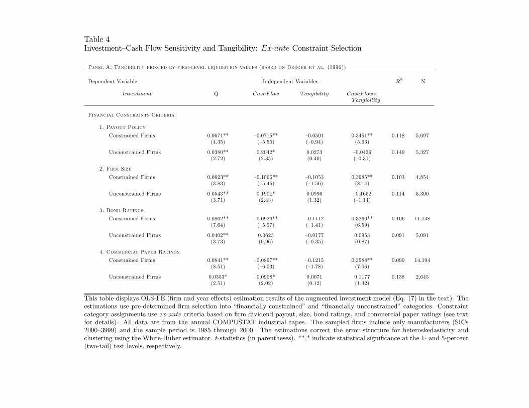
Table 4Investment�Cash Flow Sensitivity and Tangibility: Ex-ante Constraint Selection

Panel A: Tangibility proxied by firm-level liquidation values (based on Berger et al. (1996))

Dependent Variable Independent Variables R2 N

Investment Q CashF low Tangibility CashF low�Tangibility

Financial Constraints Criteria

1. Payout Policy

Constrained Firms 0.0671** �0.0715** �0.0501 0.3451** 0.118 5,697(4.35) (�5.55) (�0.94) (5.63)

Unconstrained Firms 0.0380** 0.2042* 0.0273 �0.0439 0.149 5,327(2.72) (2.35) (0.40) (�0.31)

2. Firm Size

Constrained Firms 0.0623** �0.1066** �0.1053 0.3985** 0.103 4,854(3.83) (�5.46) (�1.56) (8.14)

Unconstrained Firms 0.0543** 0.1901* 0.0996 �0.1652 0.114 5,300(3.71) (2.43) (1.32) (�1.14)

3. Bond Ratings

Constrained Firms 0.0862** �0.0926** �0.1112 0.3260** 0.106 11,748(7.64) (�5.97) (�1.41) (6.59)

Unconstrained Firms 0.0402** 0.0623 �0.0177 0.0953 0.091 5,091(3.73) (0.96) (�0.35) (0.87)

4. Commercial Paper Ratings

Constrained Firms 0.0841** �0.0897** �0.1215 0.3588** 0.099 14,194(8.51) (�6.03) (�1.78) (7.06)

Unconstrained Firms 0.0353* 0.0908* 0.0071 0.1177 0.138 2,645(2.51) (2.02) (0.12) (1.42)

This table displays OLS-FE (�rm and year e¤ects) estimation results of the augmented investment model (Eq. (7) in the text). Theestimations use pre-determined �rm selection into ��nancially constrained�and ��nancially unconstrained�categories. Constraintcategory assignments use ex-ante criteria based on �rm dividend payout, size, bond ratings, and commercial paper ratings (see textfor details). All data are from the annual COMPUSTAT industrial tapes. The sampled �rms include only manufacturers (SICs2000�3999) and the sample period is 1985 through 2000. The estimations correct the error structure for heteroskedasticity andclustering using the White-Huber estimator. t-statistics (in parentheses). **,* indicate statistical signi�cance at the 1- and 5-percent(two-tail) test levels, respectively.

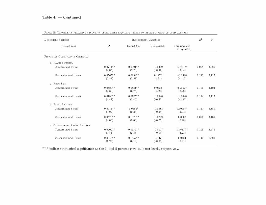
Table 4: � Continued

Panel B: Tangibility proxied by industry-level asset liquidity (based on redeployment of used capital)

Dependent Variable Independent Variables R2 N

Investment Q CashF low Tangibility CashF low�Tangibility

Financial Constraints Criteria

1. Payout Policy

Constrained Firms 0.0711** 0.0591** �0.0359 0.5781** 0.078 3,387(4.05) (2.70) (�0.41) (3.84)

Unconstrained Firms 0.0565** 0.0934** 0.1276 �0.2328 0.142 3,117(3.37) (5.58) (1.21) (�1.15)

2. Firm Size

Constrained Firms 0.0820** 0.0881** 0.0633 0.2952* 0.100 3,104(4.30) (3.75) (0.62) (2.28)

Unconstrained Firms 0.0753** 0.0725** �0.0820 �0.3448 0.114 3,117(4.42) (3.40) (�0.56) (�1.08)

3. Bond Ratings

Constrained Firms 0.0914** 0.0660* �0.0083 0.5048** 0.117 6,889(7.09) (2.36) (�0.08) (2.94)

Unconstrained Firms 0.0576** 0.1078** �0.0799 0.0607 0.092 3,169(4.03) (3.00) (�0.75) (0.28)

4. Commercial Paper Ratings

Constrained Firms 0.0900** 0.0682** �0.0127 0.4631** 0.109 8,471(7.71) (2.88) (�0.14) (3.23)

Unconstrained Firms 0.0313** 0.1552** �0.1371 0.0454 0.143 1,587(3.22) (6.19) (�0.85) (0.21)

**,* indicate statistical signi�cance at the 1- and 5-percent (two-tail) test levels, respectively.

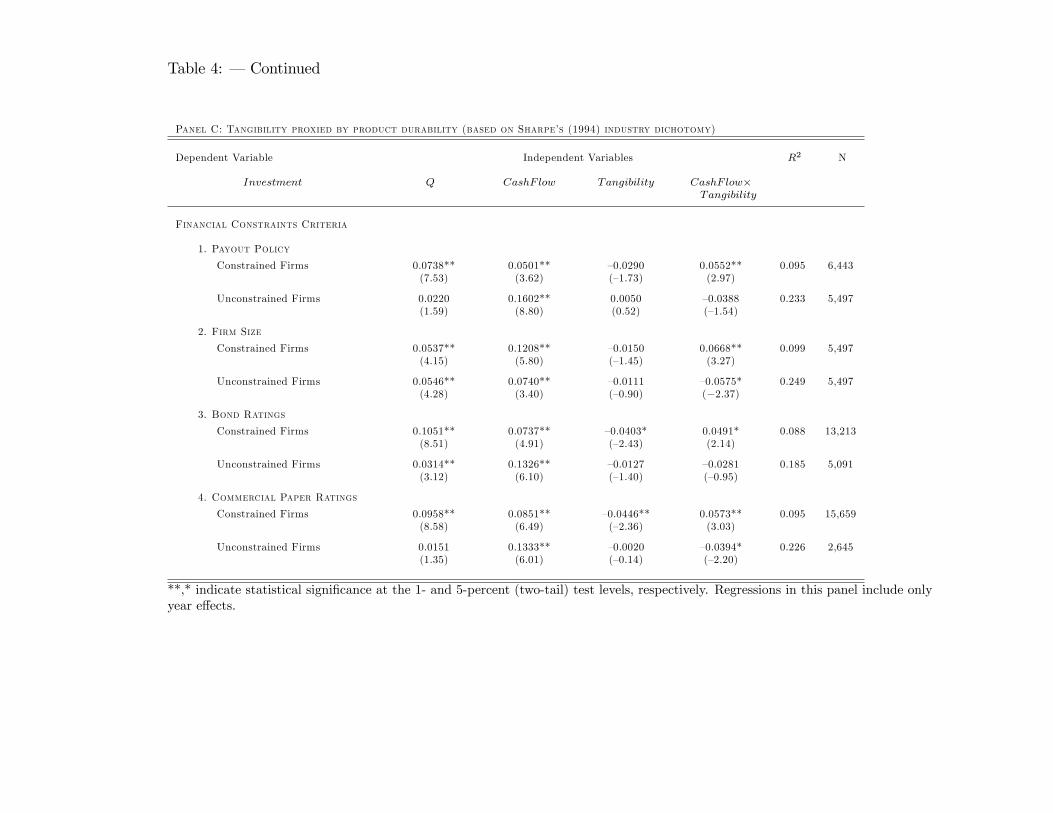
Table 4: � Continued

Panel C: Tangibility proxied by product durability (based on Sharpe�s (1994) industry dichotomy)

Dependent Variable Independent Variables R2 N

Investment Q CashF low Tangibility CashF low�Tangibility

Financial Constraints Criteria

1. Payout Policy

Constrained Firms 0.0738** 0.0501** �0.0290 0.0552** 0.095 6,443(7.53) (3.62) (�1.73) (2.97)

Unconstrained Firms 0.0220 0.1602** 0.0050 �0.0388 0.233 5,497(1.59) (8.80) (0.52) (�1.54)

2. Firm Size

Constrained Firms 0.0537** 0.1208** �0.0150 0.0668** 0.099 5,497(4.15) (5.80) (�1.45) (3.27)

Unconstrained Firms 0.0546** 0.0740** �0.0111 �0.0575* 0.249 5,497(4.28) (3.40) (�0.90) (�2.37)

3. Bond Ratings

Constrained Firms 0.1051** 0.0737** �0.0403* 0.0491* 0.088 13,213(8.51) (4.91) (�2.43) (2.14)

Unconstrained Firms 0.0314** 0.1326** �0.0127 �0.0281 0.185 5,091(3.12) (6.10) (�1.40) (�0.95)

4. Commercial Paper Ratings

Constrained Firms 0.0958** 0.0851** �0.0446** 0.0573** 0.095 15,659(8.58) (6.49) (�2.36) (3.03)

Unconstrained Firms 0.0151 0.1333** �0.0020 �0.0394* 0.226 2,645(1.35) (6.01) (�0.14) (�2.20)

**,* indicate statistical signi�cance at the 1- and 5-percent (two-tail) test levels, respectively. Regressions in this panel include onlyyear e¤ects.

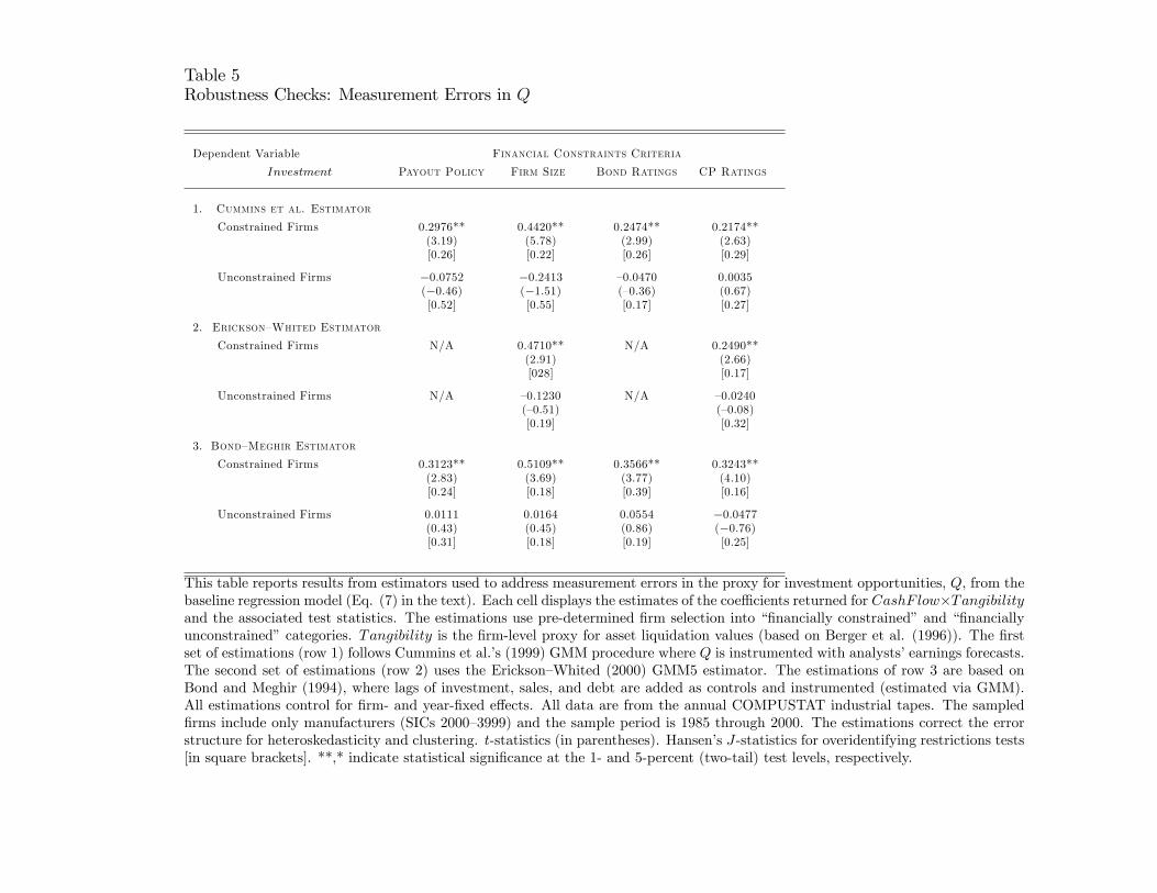
Table 5Robustness Checks: Measurement Errors in Q

Dependent Variable Financial Constraints Criteria

Investment Payout Policy Firm Size Bond Ratings CP Ratings

1. Cummins et al. Estimator

Constrained Firms 0.2976** 0.4420** 0.2474** 0.2174**(3.19) (5.78) (2.99) (2.63)[0.26] [0.22] [0.26] [0.29]

Unconstrained Firms �0.0752 �0.2413 �0.0470 0.0035(�0.46) (�1.51) (�0.36) (0.67)[0.52] [0.55] [0.17] [0.27]

2. Erickson�Whited Estimator

Constrained Firms N/A 0.4710** N/A 0.2490**(2.91) (2.66)[028] [0.17]

Unconstrained Firms N/A �0.1230 N/A �0.0240(�0.51) (�0.08)[0.19] [0.32]

3. Bond�Meghir Estimator

Constrained Firms 0.3123** 0.5109** 0.3566** 0.3243**(2.83) (3.69) (3.77) (4.10)[0.24] [0.18] [0.39] [0.16]

Unconstrained Firms 0.0111 0.0164 0.0554 �0.0477(0.43) (0.45) (0.86) (�0.76)[0.31] [0.18] [0.19] [0.25]

This table reports results from estimators used to address measurement errors in the proxy for investment opportunities, Q, from thebaseline regression model (Eq. (7) in the text). Each cell displays the estimates of the coe¢ cients returned for CashF low�Tangibilityand the associated test statistics. The estimations use pre-determined �rm selection into ��nancially constrained�and ��nanciallyunconstrained�categories. Tangibility is the �rm-level proxy for asset liquidation values (based on Berger et al. (1996)). The �rstset of estimations (row 1) follows Cummins et al.�s (1999) GMM procedure where Q is instrumented with analysts�earnings forecasts.The second set of estimations (row 2) uses the Erickson�Whited (2000) GMM5 estimator. The estimations of row 3 are based onBond and Meghir (1994), where lags of investment, sales, and debt are added as controls and instrumented (estimated via GMM).All estimations control for �rm- and year-�xed e¤ects. All data are from the annual COMPUSTAT industrial tapes. The sampled�rms include only manufacturers (SICs 2000�3999) and the sample period is 1985 through 2000. The estimations correct the errorstructure for heteroskedasticity and clustering. t-statistics (in parentheses). Hansen�s J-statistics for overidentifying restrictions tests[in square brackets]. **,* indicate statistical signi�cance at the 1- and 5-percent (two-tail) test levels, respectively.

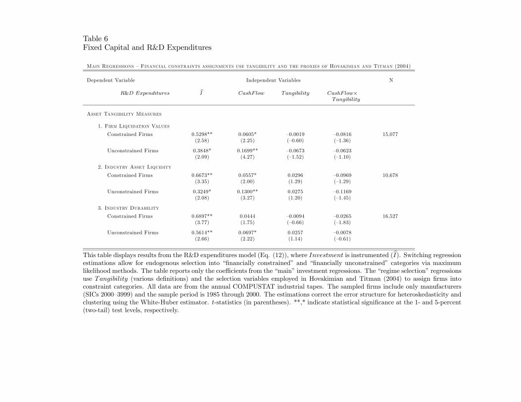
Table 6Fixed Capital and R&D Expenditures

Main Regressions �Financial constraints assignments use tangibility and the proxies of Hovakimian and Titman (2004)

Dependent Variable Independent Variables N

R&D Expenditures bI CashF low Tangibility CashF low�Tangibility

Asset Tangibility Measures

1. Firm Liquidation Values

Constrained Firms 0.5298** 0.0605* �0.0019 �0.0816 15,077(2.58) (2.25) (�0.60) (�1.36)

Unconstrained Firms 0.3848* 0.1699** �0.0673 �0.0623(2.09) (4.27) (�1.52) (�1.10)

2. Industry Asset Liquidity

Constrained Firms 0.6673** 0.0557* 0.0296 �0.0969 10,678(3.35) (2.00) (1.29) (�1.29)

Unconstrained Firms 0.3249* 0.1300** 0.0275 �0.1169(2.08) (3.27) (1.20) (�1.45)

3. Industry Durability

Constrained Firms 0.6897** 0.0444 �0.0094 �0.0265 16,527(3.77) (1.75) (�0.66) (�1.83)

Unconstrained Firms 0.5614** 0.0697* 0.0257 �0.0078(2.66) (2.22) (1.14) (�0.61)

This table displays results from the R&D expenditures model (Eq. (12)), where Investment is instrumented (bI). Switching regressionestimations allow for endogenous selection into ��nancially constrained� and ��nancially unconstrained� categories via maximumlikelihood methods. The table reports only the coe¢ cients from the �main�investment regressions. The �regime selection�regressionsuse Tangibility (various de�nitions) and the selection variables employed in Hovakimian and Titman (2004) to assign �rms intoconstraint categories. All data are from the annual COMPUSTAT industrial tapes. The sampled �rms include only manufacturers(SICs 2000�3999) and the sample period is 1985 through 2000. The estimations correct the error structure for heteroskedasticity andclustering using the White-Huber estimator. t-statistics (in parentheses). **,* indicate statistical signi�cance at the 1- and 5-percent(two-tail) test levels, respectively.