Financial Constraints and Nominal Price Rigidities

Almut Balleer, Nikolay Hristov, and Dominik Menno∗

January 9, 2017

Abstract

This paper investigates how �nancial market imperfections and the frequency of price adjustment

interact. Based on new �rm-level evidence for Germany, we document that �nancially constrained

�rms adjust prices more often than their unconstrained counterparts, both upwards and downwards.

We show that these empirical patterns are consistent with a partial equilibrium menu-cost model

with a working capital constraint. We then use the model to show how the presence of �nancial

frictions changes pro�ts and the price distribution of �rms compared to a model without �nancial

frictions. Our results suggest that tighter �nancial constraints are associated with lower nominal

rigidities, higher prices and lower output. Moreover, in response to aggregate shocks, aggregate price

rigidity moves substantially, the response of in�ation is dampened, while output reacts more in the

presence of �nancial frictions. This means that �nancial frictions make the aggregate supply curve

�atter for all calibrations considered in our model. We show that this di�ers fundamentally from

models in which the extensive margin of price adjustment is absent (Rotemberg, 1982) or constant

(Calvo, 1983). Hence, the interaction of �nancial frictions and the frequency of price adjustment

potentially induces important consequences for the e�ectiveness of monetary policy.

Keywords: Frequency of price adjustment, �nancial frictions, menu cost model

JEL-Codes: E31, E44

∗Balleer: RWTH Aachen, IIES at Stockholm University and CEPR, balleer@ewifo.rwth-aachen.de. Hristov: ifo Institute

Munich, hristov@ifo.de. Menno: Aarhus University, dmenno@econ.au.dk. We would like to thank Christoph Boehm,

Tobias Broer, Zeno Enders, Giorgio Fabbri, Andrei Levchenko, Stefan Pitschner, Morten Ravn, Andreas Schabert, Marija

Vukotic, and numerous participants at the DFG Priority Programme 1578 workshops, the ifo Macro and Survey data

workshop, SED Warsaw, VfS-Annual Conference, joint BoE, ECB, CEPR and CFM Conference on Credit Dynamics and

the Macroeconomy, ESSIM Helsinki, ICMAIF-Annual Conference 2016, CESifo Area Conference on Macro, Money and

International Finance 2016, Belgrade Young Economists Conference, and NORMAC 2016 as well as seminar participants

at the ifo Institute, Riksbank Sweden, Bundesbank, IWH Halle, and the Universities of Augsburg, Basel, Berlin, Konstanz,

Linz, Louvain-la-Neuve, Michigan and Warwick. Financial support from the DFG Priority Programme 1578 is gratefully

acknowledged.

1 Introduction

How do �nancial frictions a�ect macroeconomic outcomes? This paper investigates the interaction be-

tween �nancial frictions and the frequency of price adjustment in the economy. We document empirically

that �nancially constrained �rms adjust prices more often than their unconstrained counterparts, both

up- and downwards. We replicate this pattern in a partial-equilibrium menu cost model with a working

capital constraint. Based on this model, we then explore the cross-sectional distribution of pricing deci-

sions in response to idiosyncratic and aggregate shocks and show how it interacts with �nancial frictions.

In particular, we document that �nancial frictions impose important asymmetries in the pro�ts and the

price gap distribution of both �nancially constrained and unconstrained �rms. Based on this, we show

that aggregate price rigidity and prices increase, while output falls in the presence of �nancial frictions.

Moreover, in response to aggregate shocks, aggregate price rigidity moves substantially, the response of

in�ation is dampened, while output reacts more in the presence of �nancial frictions. Hence, �nancial

frictions potentially induce important consequences for the e�ectiveness of monetary policy.

We explore rich plant-level data for Germany: the ifo Business Survey, a monthly representative

panel of 3600 manufacturing �rms covering the years 2002-2014. The survey contains information about

the extensive margin, i.e., whether and in what direction individual �rms change prices. In addition,

the survey provides two high-frequency, direct �rm-speci�c measures of �nancial constraints: Firms give

appraisals of their access to bank credit which is the predominant way of �nancing operational costs and

investment externally in Germany. Firms also report whether they are experiencing production shortages

due to �nancial constraints. Regardless of the measure of �nancial constrainedness used and the frequency

of data, we �nd that �nancially constrained �rms adjust prices more often than unconstrained �rms. In

particular, the typical �nancially constrained �rm exhibits a signi�cantly higher frequency for both an

upward and a downward price adjustment. These patterns are also statistically signi�cant in di�erent

subperiods: before, during and after the Great Recession. To check the robustness of our results, we

exploit balance-sheet based indicators of the individual access to credit for a subset of �rms in our sample.

The existing empirical literature on the relationship between pricing decisions of �rms and �nancial

constraints is relatively scarce. It has mainly focused on price adjustment along the intensive margin1

and has also mostly not included evidence on the Great Recession period. At the same time, it mostly

relies on indirect measures of individual �nancial conditions such as the state of the business cycle or

balance sheet measures.2 Our evidence stands out since we report high-frequency survey-based measures

and evidence for a large European economy. Since we have balance sheet information for a subset of �rms

in our sample, we can compare direct and indirect measures of �nancial constraints. The study that is

closest to ours is a recent study for the US by Gilchrist et al. (2013). Based on balance sheet measures,

Gilchrist et al. also show that among price adjusters �nancially constrained �rms adjust prices up more

often than unconstrained �rms with the relationship being signi�cant only during the Great Recession.

Unlike in the current paper, they focus on the intensive margin of price adjustment rather than on the

interaction between �nancial constraints and the frequency of price changes.

Our interpretation of the empirical facts is guided by a partial-equilibrium menu cost model with

�nancial frictions which provides an explicit rationale for the interactions between �nancial constraints

and nominal rigidities. Here, we extend the standard menu-cost model with heterogeneous �rms by

adding a working capital constraint.3 In this model, �nancial frictions and price setting may a�ect each

1See for example Chevalier and Scharfstein (1996) for the US or Gottfries (2002) and Asplund et al. (2005) for Sweden.2Only Bhaskar et al. (1993) use a small-sample one time cross-sectional survey for small �rms in the UK.3In contrast, existing studies on the interaction between �nancial frictions and pricing decisions consider the intensive

margin only, i.e., the fraction of �rms that adjust prices is always equal to one, see e.g. Gilchrist et al. (2013), Gottfries

2

other in several ways. On the one hand, being �nancially constrained may a�ect the pricing decision of a

�rm: �rms with initially low prices that sell large quantities may not be able to �nance their production

inputs and may therefore �nd it optimal to scale down production and/or to adjust prices up. On the

other hand, �rms seeking to gain market share may want to lower their prices. However, by doing so,

they may run into �nancial constraints when expanding production. Finally, �rms trade-o� current and

expected future pro�ts and may be inclined to set prices such that future expected menu-costs can be

reduced (as the expected time until the next price adjustment is maximized).

We document that the presence of �nancial constraints makes the individual �rm's pro�t function

more concave in the price and introduces important asymmetries. Pro�ts fall more quickly for prices

below compared to above the constrained optimal reset price, since these prices imply rationing output

which is very costly to �rms. This means that the inaction region in which it is optimal for �rms not to

adjust prices is more narrow and more asymmetric around the optimal constrained reset price compared

to the optimal unconstrained reset price. As a result, for any given beginning-of-period price, �rms are

more likely to adjust prices. At the same time, the presence of �nancial frictions reduces the elasticity

of the optimal reset price with respect to productivity, i.e., the optimal reset price falls less strongly

with increasing productivity. Financial frictions also change the stationary distribution of beginning-of-

period prices as the price gap distribution becomes less dispersed. This distributional e�ect reduces the

frequency of price changes.

For the bulk of empirically plausible parameterizations, the width of the inaction region e�ect is

stronger than the distributional e�ect for �nancially constrained �rms compared to �nancially uncon-

strained �rms. Hence, our model replicates the empirical �nding that �nancially constrained �rms adjust

prices more often than unconstrained �rms. We also decompose this e�ect for di�erent productivity levels

of �rms and show that the frequency of price changes is generally low for intermediate productivity levels.

Moreover, most unconstrained �rms have intermediate productivity realizations. Financially constrained

�rms tend to adjust prices down very often for high productivity realizations. At the same time, many

�nancially constrained �rms have low productivity realizations at which the price adjustment (upwards)

is still substantial. It is important to note however, that the above holds in a world with �nancial fric-

tions. When comparing a world with to a world without �nancial frictions, the distributional e�ect is

very strong at all productivity levels and for all types of �rms, the unconstrained �rms in particular.

Hence, even though �nancially constrained �rms adjust their prices more often than their unconstrained

counterparts, the overall frequency of price changes falls in the presence of �nancial frictions.

To investigate the implications of �nancial frictions on the economy, we consider the responses of

average in�ation and real output to aggregate nominal demand shocks. In our partial-equilibrium model,

these shocks can be interpreted as responses of a single sector to aggregate business cycle shocks. Doing

so, we obviously ignore important general equilibrium e�ects, in particular the response of real wages.

We nevertheless believe this to be an instructive exercise as real wages might be sticky or downward

rigid in the short run. We �nd that, due to the asymmetry in the price distribution, �rms adjust

prices more often in a boom and less often in a recession when �nancial constraints are present. In

addition, due to the lower average frequency of price adjustment, the aggregate demand shock induces

a smaller change in in�ation and a stronger reaction of output relative to an economy without credit

(1991), Chevalier and Scharfstein (1996) or Lundin and Yun (2009). The literature on menu costs has in turn not focusedon �nancial frictions, e.g. Barro (1972), Caplin and Spulber (1987), Dotsey et al. (1999), Golosov and Lucas (2007) orGilchrist et al. (2013). Extensions as stochastic idiosyncratic menu costs and leptokurtic productivity shocks are analysedin Dotsey and King (2005) and Midrigan (2011) respectively. Multi-sector and multi-product versions of the model aredeveloped by Nakamura and Steinsson (2010) and Alvarez and Lippi (2014). Vavra (2013) and Bachmann et al. (2013)investigate the consequences of uncertainty shocks for the price distribution and the e�ectiveness of monetary policy.

3

market imperfections. This means that �nancial constraints alter a central trade-o� faced by the central

bank: In order to engineer an increase in in�ation by a certain amount the monetary authority needs to

generate larger changes in nominal demand. At the same time, it needs to take into account that larger

changes in nominal demand induce even stronger responses of average output. This model implication

is very similar to what has been highlighted as the �cost channel� of �nancial frictions by Gilchrist et al.

(2013). In our framework, this means that �nancial frictions decrease the slope of the aggregate supply

curve. In contrast, we show that other sources of nominal rigidities such as exogenous probabilities of

price adjustment as in Calvo (1983) or convex price adjustment costs as in Rotemberg (1982) generate

the opposite result, i.e. the inclusion of �nancial frictions generates larger in�ation and smaller output

responses to aggregate shocks with compared to without �nancial frictions. Hence, menu costs and the

associated endogenous link between the fraction of price adjusters and the presence of credit market

imperfections play a crucial role for aggregate �uctuations.

The remainder of the paper is organized as follows. Section 2 documents the data and the empirical

relationship between �nancial frictions and the price setting of �rms. Section 3 presents the model, derives

the central insights from the static model, discusses the calibration and documents the implications for

the cross-section of �rms. Section 4 documents and discusses the aggregate implications, compares the

results to alternative sources of nominal rigidities, discusses robustness of the results and considers the

special case of a �nancial recession. Section 5 concludes.

2 Empirical Evidence

2.1 Data

We use data from the ifo Business Survey which is a representative sample of 3600 plants in the German

manufacturing sector in 2002-2014. The survey starts as early as the 1950's, but our sample is restricted

by the fact that the questions about �nancial constrainedness were added in 2002. The main advantages

of the dataset relative to data used in other studies on price stickiness are twofold. First it enables us to

link individual plant's pricing decisions to both direct survey-based measures of plant-speci�c �nancial

constrainedness and to indirect proxies for the �nancial situation based on balance sheet information.

Second, the survey is conducted on a monthly basis which enables us to track important aspects of a

plant's actual behavior over time as it undergoes both phases of easy and such of subdued access to

credit while at the same time facing the alternating states of the business cycle. Since plants respond on

a voluntary basis and, thus, not all plants respond every month, the panel is unbalanced.

In particular, we have monthly information about the extensive margin of price adjustment, i.e.

whether and in what direction �rms adjust prices. More precisely, �rms answer the question: �Have

you in the last month increased, decreased or left unchanged your domestic sales prices?�.4 Since we do

not have information about the intensive margin of price adjustment in our dataset, the calibration and

implications of our model will be compared to information from other data sources (see Section 3 below).

More than 97% of the cross-sectional units in our sample are single-product plants. Additionally, some

plants �ll in a separate questionnaire for each product (product group) they produce. In what follows,

we use the terms ��rm�, �plant� and �product� interchangeably.

The ifo survey encompasses two questions regarding the �nancial constrainedness of �rms. In the

4These prices are home country producer prices and refer to the baseline or reference producer price (not to sales, etc.).Bachmann et al. (2013) have used the same dataset to assess the e�ect of uncertainty shocks on price setting. Strasser(2013) uses the dataset to study the role of �nancial frictions for the exchange rate pass through of exporting �rms.

4

monthly survey, �rms are asked about their access to bank lending: �Are you assessing the willingness of

banks to lend as restrictive, normal or accommodating?�. We �ag �rms as �nancially constrained when

they answer that bank lending is restrictive and we will use this as our baseline measure of �nancial

constraints. Note that this answer might imply that �rms experience restrictive bank lending in general,

but do not necessarily need to borrow more or have been declined credit. This means that they are

potentially not restricted in the way they invest, hire or produce.5 However, assessing the current

situation as one with restricted access to credit may still a�ect �rm behavior, e.g. via the future lending

conditions the �rm expects to face.

Bank lending is the key �nancing channel in Germany. Appendix A.1 exhibits information about

the �nancing structure in Germany in general and in the ifo dataset in particular. Generally, German

�rms show a much higher share of loans in their balance sheets than their US counterparts, while the

equity share is comparable. External �nancing through securities and bonds is marginal in Germany.

Further, a �ow-of-funds analysis of the Bundesbank documents that within equity, internal �nancing

works through retaining pro�ts, while market-�nancing plays almost no role, not even in the Great

Recession.6 Restrictions in bank lending therefore pose serious constraints to the �rms in our sample.

Below, we will additionally consider to role of �rm size, multi-products or exports for the results as these

may re�ect di�erent �nancial possibilities of �rms.

A second question in the survey relates �nancial and production constraints more closely: �Are your

domestic production activities currently constrained due to di�culties in �nancing?�. This question is

very close to the actual de�nition of �nancial constraints in the economic model that we present below.

However, it is only available at quarterly frequency. In addition, the response rate on this and other

questions about production shortages is very low. The question is only answered positively, not negatively

which means that we cannot tell apart missing data from unconstrained �rms. We will use this question

in order to explore robustness. A fraction of 84% of the �rms that qualify as restricted according to the

banking measure respond positively to the production shortage question.

Our sample exhibits an average of 32% of constrained �rms according to the banking measure and 5%

of constrained �rms according to the production measure. In Appendix A.1 we show a time-series plot

of the fraction of constrained �rms according to both measures of �nancial constraints. One can see that

the fraction of constrained �rms increases in a boom and decreases in a recession. One can also see that

the banking measure is available at monthly frequency from 2009 onwards, and semi-annually before. In

our estimations below, we interpolate all measures to monthly frequency throughout the sample.

We would like to know whether �nancially constrained and unconstrained �rms are systematically

di�erent in some important aspect. The literature has discussed that small rather than large �rms

tend to be �nancially constrained.7 For our baseline measure, our data does not exhibit this feature.

In Appendix A.1, we show that �rms that have restrictive access to bank lending are not signi�cantly

smaller than other �rms in terms of employment, sales or total assets. We also show that the fraction of

constrained �rms varies greatly between sectors.

Existing evidence on �nancial constraints is primarily based on balance sheet data rather than survey

data. For a subsample of the �rms in our survey, we have access to annual balance sheet information

and we can calculate liquidity ratios similar to Gilchrist et al. (2013).8 In Appendix A.1 we show that

5Based on a similar survey with a similar question about re�nancing conditions for Austria Fdrmuc, Hainz and Hoelzl(2016) con�rm that a �rm's own recent experience regarding credit negotiations with banks is by far the main driver of itsappraisals of banks' willingness to lend. In contrast, aggregate or sector-speci�c conditions are of minor importance.

6See DeutscheBundesbank (2013) and DeutscheBundesbank (2014).7See Carpenter et al. (1994) for an early contribution on the topic.8The data source here is the EBDC-BEP (2012): Business Expectations Panel 1/1980 12/2012, LMU-ifo Economics

and Business Data Center, Munich, doi: 10.7805/ebdc-bep-2012. This dataset links �rms' balance sheets from the Bureau

5

liquidity ratios are a little lower for �rms that are constrained according to our survey questions. The

di�erence is minimal for our baseline measure, however. The conventional balance-sheet based measure

de�nes �rms to be �nancially constrained if they are below the median liquidity ratio with respect to

all �rms in the sample. The overlap between this type of balance sheet measure and both of our survey

questions is very small (see Appendix). Generally, a low liquidity ratio can be the result of easy access

to credit, while not a�ecting production possibilities of �rms. It may therefore not measure �nancial

constraints per se. For example, consider a �rm experiencing a sudden decline in its marginal costs.

Such a �rm will typically decrease its prices and try to scale up the level of operation. If expanding

the production capacity requires external funding, the �rm may hit the upper limit of its �nancial

constraint, but may still enjoy a relatively high liquidity ratio. Hence, one may wrongly conclude that it

is �nancially unconstrained today. Below, we document that the relationship between price setting and

�nancial constrainedness does not crucially depend on the measure of �nancial constraints.

Table 1 shows the relationship between price adjustments and being �nancially constrained in our

dataset. In general few German �rms adjust their prices on a monthly basis: a little more than 20%

on average. Out of these, 10% of �rms adjust prices up and down on average (not shown in the Table).

These will be three central moments that we target when calibrating our model in Section 3 below.

In Appendix A.1, we document that there is a lot of variation in price changes and hence changes

in nominal rigidities over time. We also document that all �rms (both constrained and unconstrained

�rms) decrease prices more often and increase prices less often in a recession. Over time, �nancially

constrained �rms decrease prices more often than unconstrained �rms, regardless of the business cycle

state. While the di�erences between price increases of constrained and unconstrained �rms is small,

more unconstrained �rms leave prices constant relative to constrained �rms in a recession compared to

outside a recession. Clearly, the time series variation of pricing decisions may be driven by two facts:

the business cycle itself, sector-speci�c aspects and a possible selection of �rms over the business cycle.

Based on our estimations below, we can however exclude that these e�ects are driving the di�erences in

pricing decisions.

2.2 Estimation

In order to control for time and individual �xed e�ects, we decompose the correlation between price

changes and �nancial constrainedness using the following speci�cation

I(∆pijt Q 0) = β0 + β1FCijt + ∆pijt−1 + cj + θt + xijt + uijt. (1)

Based on this equation, we estimate independently three linear models for which the dependent variable

measures whether the prices change, increase or decrease.9 The left-hand side, I(∆pijt Q 0), is an

indicator function that takes the value 1 if the price stays constant, increases, or decreases, respectively.

The right-hand side contains the measure of being �nancially constrained, the lagged pricing decision

to control for the fact that �rms may have been a�ected by di�erent shocks previously as well as sector

and time �xed e�ects. The coe�cient β1 then measures the within-�rm variation over time between

being �nancially constrained and the probability of adjusting the price at all, up or down. Note that

this coe�cient should not be interpreted as causal, since it may well be that price adjustments in�uence

van Dyk (BvD) Amadeus database and the Hoppenstedt database to a subset of the �rms in the ifo Business Survey. SeeKleemann and Wiegand (2014) for a detailed description of this data source. Liquidity ratios are de�ned as cash and cashequivalents over total assets.

9We also considered a multinomial speci�cation. Doing so does not alter the main conclusions, see Appendix A.1 fordetails.

6

Table 1: Financial Constraints and Price Setting

unconstrained constrained

Bank lending

Fractions 0.68 0.32∆p = 0 0.80 0.76∆p < 0 0.08 0.14∆p > 0 0.13 0.10

Production shortage

Fractions 0.95 0.05∆p = 0 0.80 0.75∆p < 0 0.08 0.12∆p > 0 0.11 0.13

Source: ifo Business Survey, 2002-2014. Numbers shown are sample averages of fractions of constrained and unconstrained�rms in all �rms and fractions of price changes within unconstrained and constrained �rms. Numbers for productionshortage question are based on quarterly data, interpolated to monthly frequency.

whether a �rm is �nancially constrained or not (as is motivated in the introduction and documented in

detail in Section 3 below). Instead, this speci�cation seeks to control for variation over time, i.e., business

cycle e�ects, possible selection of �rms into being �nancially constrained or not and other aspects that

could have in�uenced the unconditional moments in Table 1.

The �rst column in Table 2 shows the baseline results for our bank lending measure of �nancial con-

straints. Financially constrained �rms adjust prices more often than unconstrained �rms, the di�erence

in probability is about 4%. This di�erences is composed of �nancially constrained �rms increasing prices

about 1% more often and decreasing prices about 3% more often than unconstrained �rms. All of these

di�erences are highly signi�cant. The Table documents that the results are robust to various subsam-

ples. Small and medium sized �rms may be particularly a�ected by restricted bank lending, exporting

�rms may be less a�ected. West German �rms are potentially less a�ected by �nancial frictions and

single-product �rms may be less able to shift funds to avoid restrictions. In addition, we consider two

subsamples that end and start before and after the Great Recession period respectively. Our results are

robust to all of these subsamples.

Appendix A.1 shows further results investigating robustness along a number of dimensions. For

example, we add various control variables that could a�ect both price setting and whether �rms are

�nancially constrained or not. These include �rm size, receiving wage subsidies in the form of short-time

work programmes, lagged and current assessment of the state of business, current assessment of the state

of orders and future assessment of commercial operations. All of these variables stem from the ifo survey

and are answered qualitatively according to three categories: improved, unchanged, worsened. We also

conduct robustness with respect to di�erent speci�cations. Among others, we add seasonal (quarterly)

�xed e�ects and an interaction term between sector j and seasonal �xed e�ects. We further cluster the

standard errors at the sectoral level and allow for product-speci�c (i.e. individual) �xed e�ects rather

than sectoral �xed e�ects. In order to investigate possible e�ects of attrition of the sample, we consider a

long-coverage panel (�rms are in panel at least 8 years) and a completely-balanced panel. Furthermore,

in the Appendix we document that our results do not depend on the speci�cation being linear, as a logit

model estimation leaves the results virtually unchanged.

We have replicated all of the above results using our production constraint measures instead of the

7

Table 2: Financial Constraints and Price Setting: Subsample robustness

baseline SMEs west exporting post 2009 pre 2009 single product

→ -0.036*** -0.048*** -0.037*** -0.036*** -0.036*** -0.034*** -0.036***(0.000) (0.000) (0.000) (0.000) (0.000) (0.000) (0.000)

↑ 0.008*** 0.016*** 0.009*** 0.009*** 0.008*** 0.009** 0.008***(0.000) (0.000) (0.000) (0.000) (0.000) (0.011) (0.000)

↓ 0.028*** 0.032*** 0.028*** 0.027*** 0.029*** 0.025*** 0.028***(0.000) (0.000) (0.000) (0.000) (0.000) (0.000) (0.000)

Observations 180871 77130 146647 144441 150774 30097 179589

Notes: Survey dataset. Sample: 2002:1 - 2014:12. OLS estimation with time t and sector j �xed e�ects. Consideringsubsamples: small and medium-sized �rms only (50-250 employees), west only, exporting �rms only, before and after 2009,single product �rms. Results including very small �rms (below 250) are not shown in the table, but available upon request.Standard errors in parentheses, *** p < 0.01, ** p < 0.05, * p < 0.1.

bank lending measure for �nancial constrainedness. The results are shown in the Appendix. Generally,

the di�erence in the frequency of price adjustment between �nancially constrained and unconstrained

�rms is slightly larger in this measure. As before, �nancially constrained �rms adjust prices more often

than unconstrained �rms, but the di�erence is now equally driven by upward as by downward price

adjusters.

In a related paper, Gilchrist et al. (2013) show that US �rms that are �nancially constrained increase

prices more often than their unconstrained counterparts, but do not decrease their prices more often.

While the �rst �nding is supported using our estimation, the second �nding is not. A potential source of

this di�erence is the measure of �nancial constrainedness of �rms. While we use direct survey questions

to identify �nancially constrained �rms, Gilchrist et al. employ an indirect measure based on balance

sheet information of �rms. In the Appendix we show results when using the liquidity ratio (measured as

described above) in order to measure �nancial constrainedness. In line Gilchrist et al. (2013), constrained

�rms are those with liquidity ratios below the median value of all �rms. Our analysis shows that our

results support the results by Gilchrist et al. (2013) as �nancially constrained �rms change their prices

more often. Constrained �rms increase and decrease prices more often, but only the price increases are

statistically signi�cant. Note that potentially, our results could be very di�erent from Gilchrist et al.

(2013), since we consider a central European economy, the manufacturing sector only and many small

�rms in addition to large publicly traded �rms.

3 Model

In this section, we develop a simple partial-equilibrium model which replicates the empirical facts pre-

sented in the previous section. In particular, the model combines menu costs as a source of price rigidity

with a working capital constraint as a source of a �nancial friction. Section 3.1 presents the model and

Section 3.2 develops the economic intuition based on a static version of the model. Section 3.3 presents

the calibration and quantitative results of the dynamic model.

8

3.1 Baseline Model

Our model consists of a �rm's problem only. There is a continuum of �rms in the economy indexed by

i. Each �rm produces using a linear technology

yit = zithit.

Here, yit denotes the output of the �rm in period t, zit denotes the productivity of the �rm's labor input

in period t, and hit is the amount of labor hired by the �rm in period t. The logarithm of �rm-speci�c

productivity follows an exogenous AR(1), or

log(zit) = ρz log(zit−1) + εit. (2)

We assume that demand cit for the good produced by �rm i in period t is given by

cit =

(pitPt

)−θCt, (3)

where pit is the nominal price the �rm charges in period t, Pt denotes the aggregate price level in period t,

and Ct determines the potential total size of the market for the �rms' goods in period t. The parameter θ

is the elasticity of substitution between di�erent goods.10 Aggregate consumption Ct and the aggregate

nominal price level Pt are exogenously given. We assume that nominal total demand St = PtCt follows

an exogenous stochastic process. In line with Nakamura and Steinsson (2008), the logarithm of nominal

demand �uctuates around a trend:

log(St) = µ+ log(St−1) + ηt,

where µ is the average nominal demand growth rate in the economy.11

Working hours are hired at a real wage w. Following Nakamura and Steinsson (2008), w is assumed

to be constant and equal to

w =Wt

Pt=θ − 1

θ, (4)

where Wt denotes the nominal wage in period t.12

The �rst friction included in our theoretical set-up is a standard menu-cost. That is, the �rm has to

hire an extra �xed amount of labor f in case it decides to adjust its price. We assume that the �xed

cost f has to be paid at the end of the period after revenues have been realized.

The second friction is a �nancial constraint in the form of a working capital constraint, i.e., we assume

that payments of wages have to be made prior to the realization of revenues. Accordingly, the �rm faces

a cash �ow mismatch during the period and has to raise funds amounting to lit = whit in the form of

10The demand function re�ects the optimal decision of the consumer if her consumption basket is given by the CESindex:

C =

(∫ 1

i=0ct(i)

θθ−1 di

) θ−1θ

.

11In the numerical simulations we assume for simplicity that the size of the market Ct = C = 1 is constant over time.This is without loss of generality in this partial equilibrium setting. As a consequence, the shock speci�cation for nominaldemand is equivalent to assuming that the logarithm of the price level follows a random walk.

12We use this normalization for simplicity, it is not essential for the quantitative results. The expression of the real wageabove arises in the steady state of a general equilibrium model with a linear aggregate production function depending onlyon labor input and no �nancial constraint, monopolistic competition among �rms in the goods market, and a good-speci�cdemand function given by (3).

9

an intra-period loan. However, the �rm cannot borrow more than the a fraction of the sum of the real

liquidation value of its capital plus its sales.13

whit ≤ ξ(kit +pitPtzithit). (5)

Here, ξ is the fraction of the real value of capital (kit) plus real sales that �rms can pledge as collateral

to lenders. In principle, we can allow kit to be a �rm-speci�c choice variable. In the baseline model,

however, we abstract from heterogeneous availability of collateral across �rms and assume that capital

is �xed, kit = k = 1 ∀t. The parameter ξ is a constant and can be interpreted as the expected real

liquidation value of capital and sales in the economy.14

Firms start the period with a given nominal price pit and observe the exogenous realizations of the

aggregate nominal price level Pt as well as idiosyncratic shocks to productivity zit, respectively. Before

producing, they choose whether to change the price to qit 6= pit or to leave the nominal price unchanged.

In case the �rm is unconstrained, given the new price, the demand function then pins down the desired

level of output and the necessary amount of labor associated with that level of output. The �nancial

constraint, in turn, determines whether the desired demand and therefore output level is feasible or

not. If not, the �nancial constraint pins down the amount of labor that can be used for production and

therefore determines the output level. In case the �rm leaves the price unchanged, �nancially constrained

�rms might �nd it optimal to ration supply, in the sense that the �nancially constrained �rm does not

supply the amount demanded at the given price.

The formal structure of the �rm's optimization problem is as follows: Given (pit, Pt, zit), the �rm's

real pro�t stream each period is given by

Πit =

(pitPt− w

zit

)zithit. (6)

The associated value function is

V (pit/Pt, zit) = max{V a(zit), Vna(pit/Pt, zit)} (7)

with

V na(pit/Pt, zit) = maxhit

(pitPt− w

zit

)zithit + βEtV (pit/Pt+1, zit+1)

s.t. zithit ≤ pitPt

−θC

whit ≤ ξ(1 + pitPtzithit)

(8)

13As in Jermann and Quadrini (2012), we assume that debt contracts are not enforceable as the �rm can default. Defaulttakes place at the end of the period before the intra-period loan has to be repaid. In case of default, the lender has theright to liquidate the �rm's assets. However, the loan li represents liquid funds that can be easily diverted by the �rm incase of default. The implicit assumption is that �rms can divert parts of their revenues, so lenders can only access partξ of the value of the �rm's capital stock plus its current cash-�ow. The lower the resale value of capital and the morecash-�ow the �rm can divert, the lower the recovery value of the lenders in case of default. The working capital constraintcan therefore be viewed as an enforcement constraint.

14In Appendix A.7, we present a model version with idiosyncratic �nancial shocks, where we allow ξ to be time-varyingand to follow an idiosyncratic exogenous stochastic process.

10

and

V a(pit/Pt, zit) = maxqit 6=pit,hit

(qitPt− w

zit

)zithit − wf + βEtV (qit/Pt+1, zit+1)

s.t. zithit ≤ qitPt

−θC

whit ≤ ξ(1 + qitPtzithit)

(9)

where V a and V na are the �rm's value functions in the case the �rm adjusts its nominal price (V a)

or leaves the nominal price unchanged (V na), respectively. The �x cost f needs to be paid if the �rm

decides to change its price. Note that through yit ≤ cit we allow the �rm to produce less than the

amount of goods demanded.

3.2 Special Case: Myopic Firms

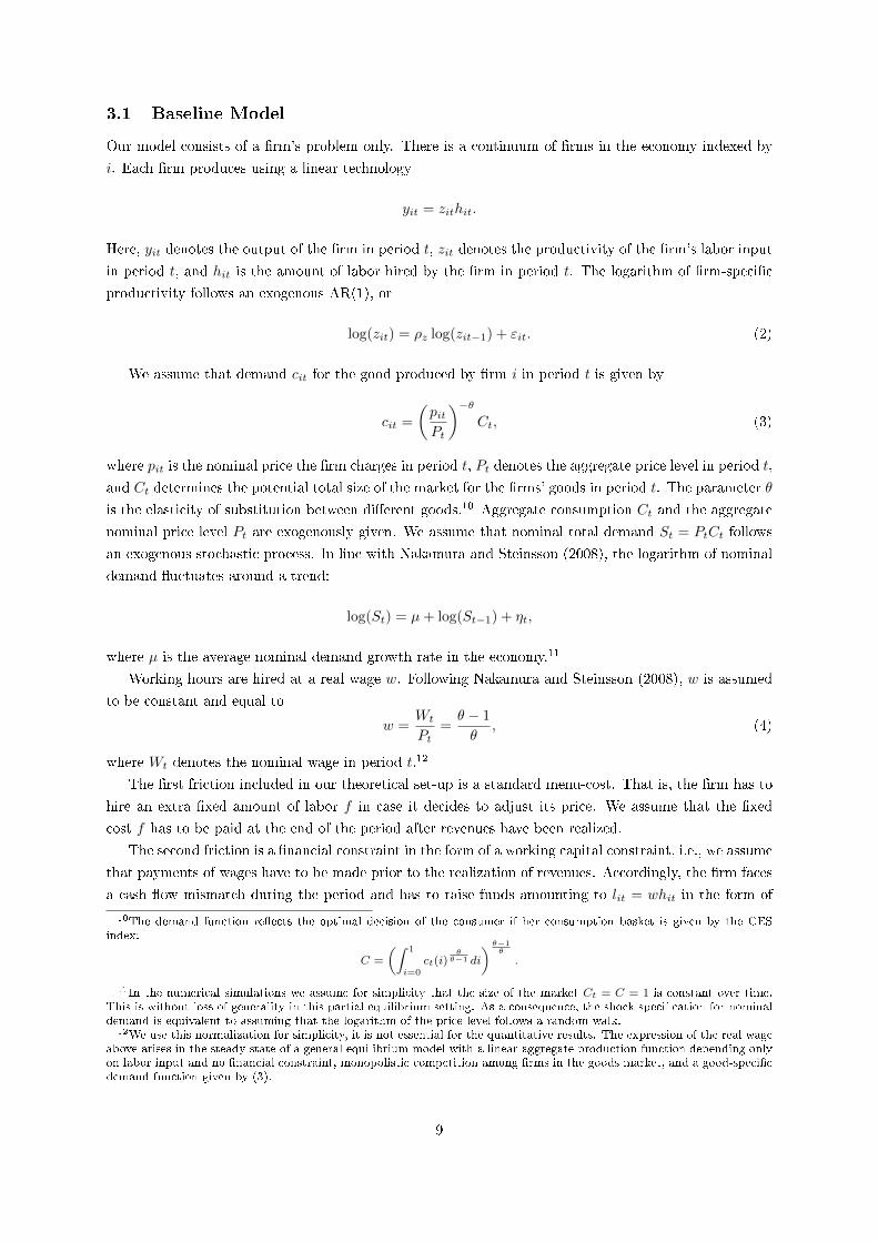
The most important insights from the model can be discussed in a simpler version of the model where

�rms are perfectly myopic, or β = 0. To enhance readability we drop time indices wherever appropriate.

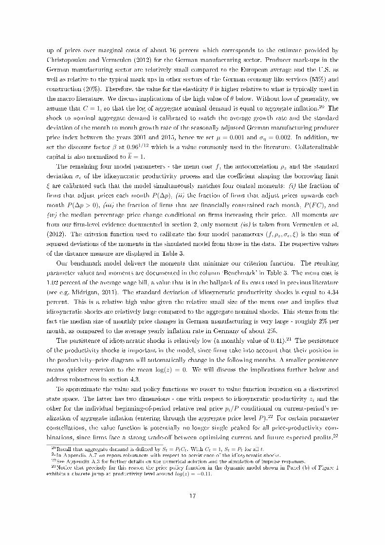
When �rms adjust their price and are �nancially unconstrained, their optimal reset price is given by

quc

P=

θ

θ − 1

w

z=

1

z, (10)

where the last equation follows from the de�nition of the real wage. Hence, �nancially unconstrained

�rms optimally charge a constant mark-up over marginal costs. Figure 1 exhibits the relationship between

the real optimal price quc/P and productivity z (blue dashed line).

In Appendix A.2 we show that if the �rm decides to adjust the price, demand is always satis�ed with

equality, independent of whether the �rm is �nancially constrained or not. Hence, when the �nancial

constraint is binding, the optimal reset price is given by:

qfc

P=

(1 + µ)

(1 + µξ)

θ

θ − 1

w

z(11)

where µ ≥ 0 is the Lagrangian multiplier associated with the �nancial constraint. This means that

the �nancially constrained �rm charges a mark-up over marginal costs w/z that is larger than the

mark-up of unconstrained �rms whenever µ is strictly positive. Further, it can be shown that µ is

increasing in productivity whenever ξ < 1.15 Accordingly, any increase in productivity has two opposing

e�ects on the �nancially constrained �rms' e�ective marginal costs: it decreases them via the standard

marginal cost channel by reducing the term w/z but it also increases them via the Lagrangean multiplier

µ as the borrowing constraint becomes more painful. Consequently, the elasticity of the �nancially

constrained optimal price qfc with respect to productivity z is smaller than (or at most as large as) the

corresponding elasticity of the optimal price without a �nancial constraint quc.16 Figure 1 illustrates

this result graphically: the black dashed line displays price-productivity combinations for which both

the �nancial constraint and the �rm's demand schedule is binding. This means that price-productivity

combinations exactly on as well as below the black dashed line are associated with a binding �nancial

constraint, price-productivity combinations above the black dashed line imply that the constraint is slack.

Note that to the right of the intersection between the black and the blue dashed line, the unconstrained

15Henceforth we will assume that this condition is satis�ed. See Appendix A.2 for a formal proof.16Appendix A.2 we show that revenues per unit labor employed qz are increasing in productivity. This means that the

elasticity of the price changes with respect to productivity changes is less than unity for �nancially constrained �rms, whileit is equal to unity for unconstrained �rms).

11

Figure 1: Pricing policy function

(a) Myopic �rms (β = 0)

-0.15

-0.10

-0.05

0.00

0.05

0.10

0.15

-0.15 -0.10 -0.05 0.00 0.05 0.10 0.15

log(r

eal price)

log(productivity)

price adjustment thresholds model with FC

non binding FC

binding FC

(b) Dynamic Model (benchmark)

-0.08

-0.06

-0.04

-0.02

0.00

0.02

0.04

0.06

0.08

0.10

0.12

0.14

0.16

0.18

-0.20 -0.15 -0.10 -0.05 0.00 0.05 0.10 0.15 0.20

log(r

eal price)

log(productivity)

price adjustment thresholds model with FC

non binding FC

binding FC

Notes: The x-axis displays the logarithm of the productivity levels zi and the y-axis shows the logarithm of the real price of the�rm pi = pi/P . Panel (a) shows the policy function in the model with myopic �rms, hence shutting down the intertemporalchannel. The corresponding calibration can be found in the robustness Section in the Appendix A.7. Panel (b) shows the policyfunction for the benchmark calibration of the dynamic model, see Table 3. In both Panels, the blue dashed line is the optimalreset price in case there is no �nancial constraint. The green lines limit the inaction region in the model without �nancial friction:A �rm with a pair (z, p) in the interval spanned by the green lines will optimally not adjust its price. The dashed black line is themaximum feasible price of a �rm that is �nancially constrained and adjusting its price (hence, the price where both the �nancialconstraint and demand are binding with equality). The red dashed line displays the optimal reset price in the model with �nancialconstraint. The purple lines limit the inaction region in the model with �nancial constraint.

pro�t maximum can no longer be achieved. For each productivity level, the red line displays the optimal

reset price in the model with �nancial constraint.

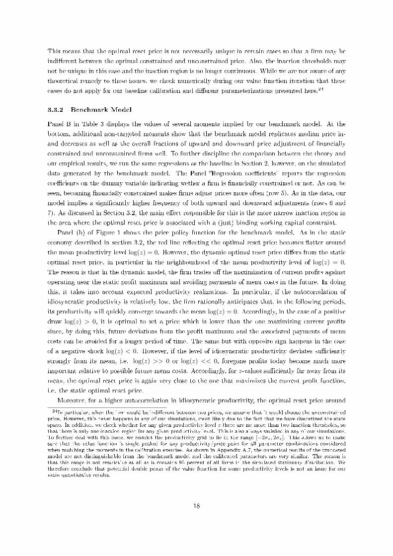
With menu costs, �rms trade o� the gain in revenue from changing the price and the cost of adjusting

the price. That gain is determined by the curvature of the pro�t function, especially in the neighbourhood

of the optimal reset price where most �rms will be located. The higher the curvature, the larger the

pro�t losses for prices away from the optimal reset prices and, hence the stronger the incentives to pay

the menu costs in order to adjust the price. Accordingly, �rms will adjust prices more frequently (as a

reaction to smaller shocks) if their pro�t function declines more steeply to the left and to the right of

the optimal reset price.

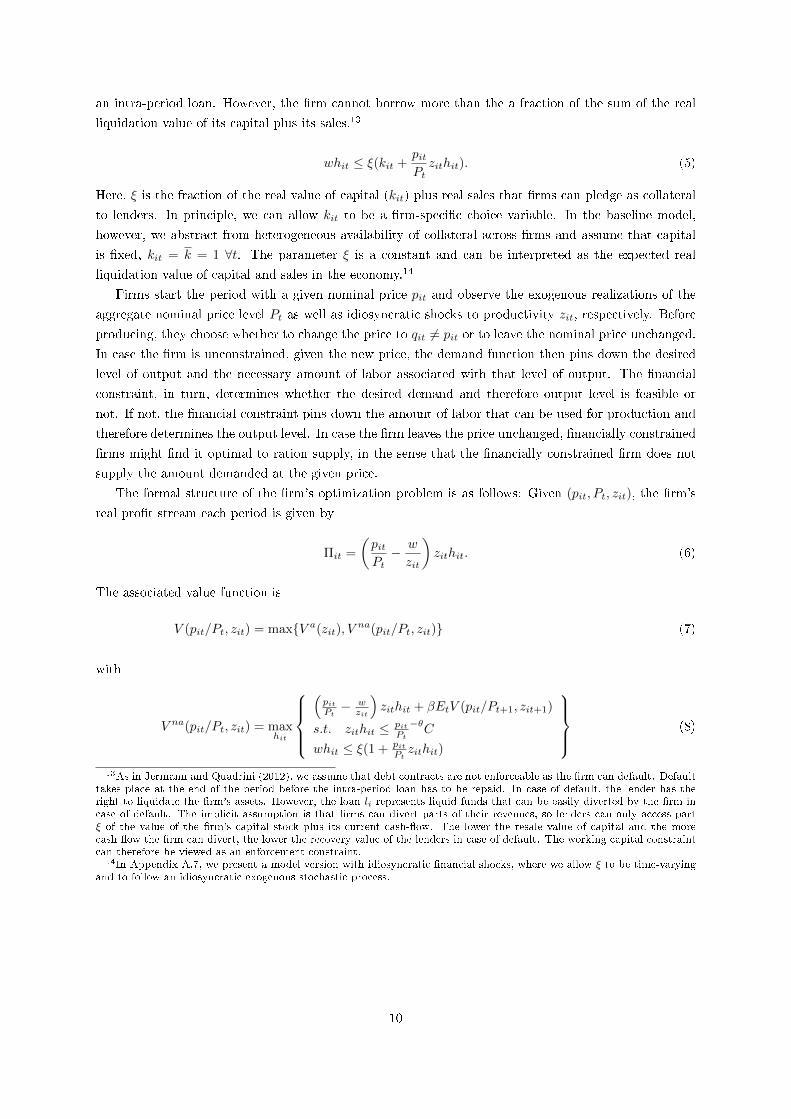
The introduction of the working capital constraint a�ects the behavior of an individual �rm by

changing the shape of its pro�t function. This is illustrated in Figure 2 for an exemplary productivity

level of log(z) = 0. In Panel (a), the concave solid blue line corresponds to the pro�t of a �nancially

unconstrained �rm as a function of the logarithm of its real price p. The pro�t function has its maximum

at p = 1 which corresponds to the optimal price in a world with fully �exible prices. The vertical dashed

lines around the maximum mark the inaction region: only �rms whose real prices lie outside the inaction

region, e.g. due to trend in�ation or the realization of exogenous shocks, will adjust their price towards

the pro�t maximum. Firms whose prices are still within the region spanned by the dashed vertical lines

will not adjust their price as in that case, the gain in pro�ts would be smaller than the menu-cost. Pro�t

functions for di�erent productivity levels are shown in Figure A.4 in Appendix A.4. The inaction regions

for all di�erent price-productivity combinations are also depicted by the area in between the green lines

in Figure 1.

Panel (b) in Figure 2 shows pro�ts in an economy without �nancial frictions (solid blue) and with

�nancial frictions (dashed red) for the same level of productivity log(z) = 0. The red pro�t function

displays a kink at the price where both the �nancial constraint and demand hold with equality. As shown

in the Appendix, this point corresponds to the constrained optimal reset price in the myopic model (for

productivity level log(z) = 0). For prices higher than the price at (or to the right of) the kink, the

12

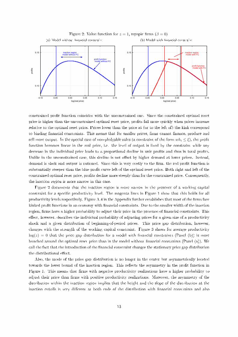
Figure 2: Value function for z = 1, myopic �rms (β = 0)

(a) Model without �nancial constraint

0.10

0.15

-0.10 -0.05 0.00 0.05 0.10 0.15

pro

fits

log(real price)

profit function model without FC

inaction region model without FC

(b) Model with �nancial constraint

0.10

0.15

-0.10 -0.05 0.00 0.05 0.10 0.15

pro

fits

log(real price)

profit function model with FC

inaction region model with FC

constrained pro�t function coincides with the unconstrained one. Since the constrained optimal reset

price is higher than the unconstrained optimal reset price, pro�ts fall more quickly when prices increase

relative to the optimal reset price. Prices lower than the price at (or to the left of) the kink correspond

to binding �nancial constraints. This means that for smaller prices, �rms cannot �nance, produce and

sell more output. In the special case of non-pledgable sales (a constraint of the form whi ≤ ξ), the pro�tfunction becomes linear in the real price, i.e. the level of output is �xed by the constraint while any

decrease in the individual price leads to a proportional decline in unit pro�ts and thus in total pro�ts.

Unlike in the unconstrained case, this decline is not o�set by higher demand at lower prices. Instead,

demand is slack and output is rationed. Since this is very costly to the �rm, the red pro�t function is

substantially steeper than the blue pro�t curve left of the optimal reset price. Both right and left of the

constrained optimal reset price, pro�ts decline more steeply than for the constrained price. Consequently,

the inaction region is more narrow in this case.

Figure 2 documents that the inaction region is more narrow in the presence of a working capital

constraint for a speci�c productivity level. The magenta lines in Figure 1 show that this holds for all

productivity levels respectively. Figure A.4 in the Appendix further establishes that most of the �rms face

kinked pro�t functions in an economy with �nancial constraints. Due to the smaller width of the inaction

region, �rms have a higher probability to adjust their price in the presence of �nancial constraints. This

e�ect, however, describes the individual probability of adjusting prices for a given size of a productivity

shock and a given distribution of beginning-of-period prices. This price gap distribution, however,

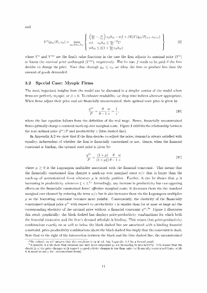
changes with the strength of the working capital constraint. Figure 3 shows for average productivity

log(z) = 0 that the price gap distribution for a model with �nancial constraints (Panel (b)) is more

bunched around the optimal reset price than in the model without �nancial constraints (Panel (a)). We

call the fact that the introduction of the �nancial constraint changes the stationary price gap distribution

the distributional e�ect.

Also, the mode of the price gap distribution is no longer in the center but asymmetrically located

towards the lower bound of the inaction region. This re�ects the asymmetry in the pro�t function in

Figure 1. This means that �rms with negative productivity realizations have a higher probability to

adjust their price than �rms with positive productivity realizations. Moreover, the asymmetry of the

distribution within the inaction region implies that the height and the slope of the distribution at the

inaction cuto�s is very di�erent at both ends of the distribution with �nancial constraints and also

13

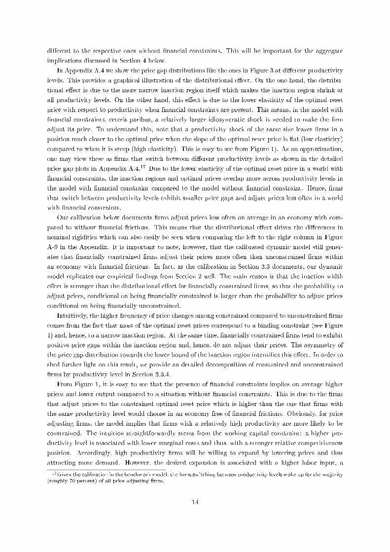
di�erent to the respective ones without �nancial constraints. This will be important for the aggregate

implications discussed in Section 4 below.

In Appendix A.4 we show the price gap distributions like the ones in Figure 3 at di�erent productivity

levels. This provides a graphical illustration of the distributional e�ect. On the one hand, the distribu-

tional e�ect is due to the more narrow inaction region itself which makes the inaction region shrink at

all productivity levels. On the other hand, this e�ect is due to the lower elasticity of the optimal reset

price with respect to productivity when �nancial constraints are present. This means, in the model with

�nancial constraints, ceteris paribus, a relatively larger idiosyncratic shock is needed to make the �rm

adjust its price. To understand this, note that a productivity shock of the same size leaves �rms in a

position much closer to the optimal price when the slope of the optimal reset price is �at (low elasticity)

compared to when it is steep (high elasticity). This is easy to see from Figure 1). As an approximation,

one may view these as �rms that switch between di�erent productivity levels as shown in the detailed

price gap plots in Appendix A.4.17 Due to the lower elasticity of the optimal reset price in a world with

�nancial constraints, the inaction regions and optimal prices overlap more across productivity levels in

the model with �nancial constraint compared to the model without �nancial constraint. Hence, �rms

that switch between productivity levels exhibit smaller price gaps and adjust prices less often in a world

with �nancial constraints.

Our calibration below documents �rms adjust prices less often on average in an economy with com-

pared to without �nancial frictions. This means that the distributional e�ect drives the di�erences in

nominal rigidities which can also easily be seen when comparing the left to the right column in Figure

A-9 in the Appendix. It is important to note, however, that the calibrated dynamic model still gener-

ates that �nancially constrained �rms adjust their prices more often than unconstrained �rms within

an economy with �nancial frictions. In fact, as the calibration in Section 3.3 documents, our dynamic

model replicates our empirical �ndings from Section 2 well. The main reason is that the inaction width

e�ect is stronger than the distributional e�ect for �nancially constrained �rms, so that the probability to

adjust prices, conditional on being �nancially constrained is larger than the probability to adjust prices

conditional on being �nancially unconstrained.

Intuitively, the higher frequency of price changes among constrained compared to unconstrained �rms

comes from the fact that most of the optimal reset prices correspond to a binding constraint (see Figure

1) and, hence, to a narrow inaction region. At the same time, �nancially constrained �rms tend to exhibit

positive price gaps within the inaction region and, hence, do not adjust their prices. The asymmetry of

the price gap distribution towards the lower bound of the inaction region intensi�es this e�ect. In order to

shed further light on this result, we provide an detailed decomposition of constrained and unconstrained

�rms by productivity level in Section 3.3.4.

From Figure 1, it is easy to see that the presence of �nancial constraints implies on average higher

prices and lower output compared to a situation without �nancial constraints. This is due to the �rms

that adjust prices to the constrained optimal reset price which is higher than the one that �rms with

the same productivity level would choose in an economy free of �nancial frictions. Obviously, for price

adjusting �rms, the model implies that �rms with a relatively high productivity are more likely to be

constrained. The intuition straightforwardly stems from the working capital constraint: a higher pro-

ductivity level is associated with lower marginal costs and thus, with a stronger relative competitiveness

position. Accordingly, high productivity �rms will be willing to expand by lowering prices and thus

attracting more demand. However, the desired expansion is associated with a higher labor input, a

17Given the calibration in the benchmark model, the �rms switching between productivity levels make up for the majority(roughly 70 percent) of all price adjusting �rms.

14

Figure 3: Price-gap distribution

(a) Myopic �rms (β = 0), no �nancial constraint (b) Myopic �rms (β = 0), with �nancial constraint

(c) Dynamic model (benchmark), no �nancial constraint (d) Dynamic model (benchmark), with �nancial constraint

Notes: The histograms display the distribution of the price gap, de�ned as the actual (pre-adjustment) price minus the optimalreset price, or log(pi) − log(p∗i ), where p∗i is �rm i's optimal reset price and pi is �rm i's price before price adjustment. Thesolid vertical lines mark the inaction region for a �rm with average productivity (i.e. log(z) = 0) in the model with and without�nancial constraint, respectively. The dashed line at zero shows the location of the optimal reset price. The dotted lines in Panels(b) and (d) are the same as the vertical solid lines for the 'No FC'-model shown in Panels (a) and (c), respectively.

higher wage bill, a higher level of borrowing and a higher likelihood of being constrained. The models

proposed by Cooley and Quadrini (2001), Azariadis and Kaas (2012), Buera et al. (2013), Khan and

Thomas (2013), Midrigan and Xu (2014) also predict a positive relationship between the level of id-

iosyncratic productivity and the likelihood of being constrained � conditional on the �rm speci�c capital

stock. In these models, �rms receiving a sequence of favourable productivity shocks tend to accelerate

the accumulation of capital which, in the long run, enables them to outgrow the credit constraint. This

mechanism is absent here as capital is assumed to be �xed.

There are three reasons why we abstract from a more complicated setup than presented here. First,

our model already delivers rich predictions about the relationship between productivity and being �-

nancially constrained. On the one hand, the prediction that more productive �rms are the ones that

are �nancially constrained only applies to �rms that optimally choose to adjust their price. On the

other hand, among the �rms that optimally decide not to adjust the price, the relationship is reversed:

relatively less productive �rms will be �nancially constrained. These are �rms that draw a negative

productivity shock that is large enough to make their �nancial constraint bind (due to their increased

15

wage bill) but not large enough to drive them out of the inaction region, so they do not �nd it optimal to

adjust the price.18 Second, in the dynamic version of our model, Figure 1 documents that both �rms with

low and high productivity levels will end up being �nancially constrained even when adjusting the price.

Third, as we will show below, the aggregate implications do not depend on whether more productive

or less productive �rms are likely to be constrained. Instead, the e�ect of aggregate shocks depends on

which �rms select into adjustment, which depends on the width of the inaction region, the distributional

e�ect and the asymmetry of the price gap distribution within the inaction region. It is important to not

that, as we discussed above, the presence of �nancial frictions changes the desired price gap distribution

for all �rms, i.e. for both �nancially constrained and unconstrained �rms.

Figures 1, 2 and 3 display the results of the static model for speci�c model parameters that align

with our benchmark calibration discussed in Section 3.3. These parameters a�ect the di�erences between

the model with and without �nancial constraints and therefore the aggregate implications discussed in

Section 4. For example, the more symmetric the pro�ts without �nancial constraints, the larger the e�ect

from introducing asymmetries associated with the �nancial constraint. In Appendix A.7 we show that

a lower value for the demand elasticity θ increases the symmetry of the pro�t function of unconstrained

�rms and makes the pro�t function �atter and the inaction region wider. In other words, the impact

of �nancial constraints is expected to be larger in industries with lower elasticity of substitutions. Also,

when sales can be pledged as collateral as in our benchmark model, the elasticity of the constrained

optimal reset price with respect to productivity decreases less compared to a situation in which sales are

non pledgable. This will play a role for ability of the model to match the data moments.19

3.3 Dynamic Model

In the previous section, we have documented that the interaction between �nancial frictions and the

pricing decisions of �rms works in both directions. On the one hand, the presence of the credit constraint

a�ects the pro�t function and thus the policy function of �rms by changing the location and the width

of the inaction region. The presence of credit constraints also a�ects the price gap distribution of �rms.

On the other hand, the optimal pricing decision determines whether the �rm will end up facing a binding

or a slack �nancial constraint. In a dynamic set-up with forward looking �rms (0 < β < 1), �rms now

trade-o� the e�ect of their pricing decision on current and expected pro�ts. Unlike in the model with

myopic �rms, the �ex-price optimum in a dynamic economy does no longer necessarily coincide with the

maximum of the current pro�t function. As Figure 1 shows, the optimal constrained and unconstrained

reset prices di�er in the static and the dynamic model. As a consequence, �rms are �nancially constrained

or unconstrained at di�erent productivity-price combinations in both versions of the model. The presence

and size of these e�ects depends on the calibration of the model. Below, we discuss how the calibration

a�ects the policy functions of the dynamic model in detail.

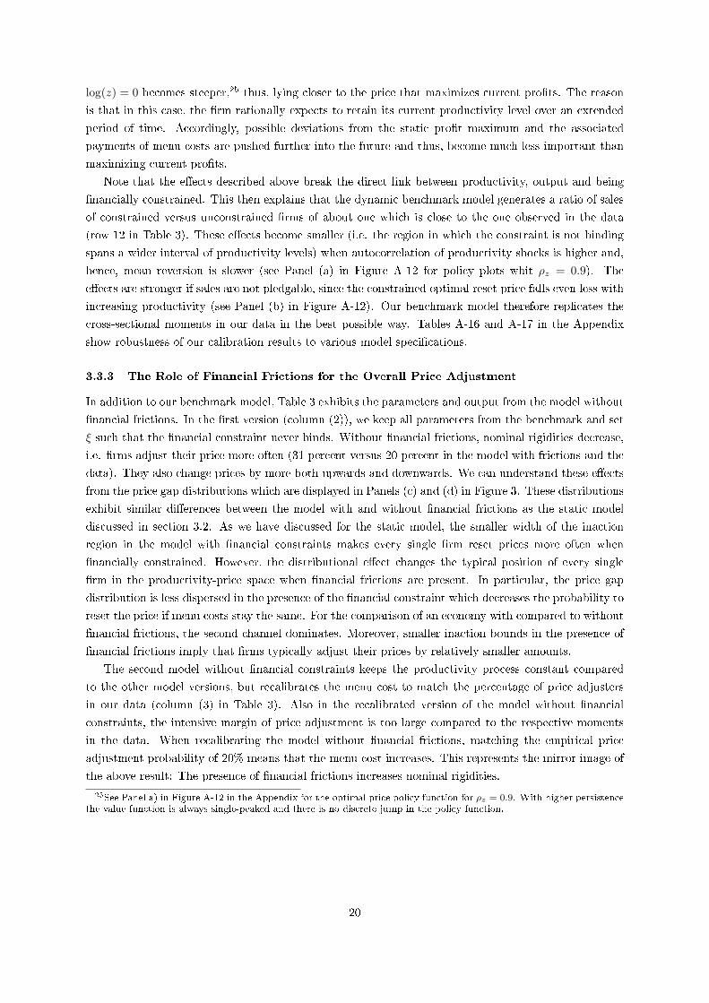
3.3.1 Calibration and Parametrization

We assume that time is measured in months which is consistent with the frequency of our data. The

elasticity of substitution between individual goods θ is set to 7.25. This value implies an average mark-

18See Appendix A.2 for a formal proof of these claims.19We have also conducted robustness with respect to decreasing returns and di�erent values of the super-elasticity using

the Kimball (1995) aggregator. Both, more decreasing returns and higher values for the super-elasticity are associated with�atter optimal price schedules for unconstrained �rms, �atter in the sense that �rms respond less to idiosyncratic shocks.As a consequence, the di�erence between a world with and without �nancial constraint is lower. However, all these modelsperformed worse in matching the micro data moments when compared to the benchmark with CES demand schedule andconstant returns.

16

up of prices over marginal costs of about 16 percent which corresponds to the estimate provided by

Christopoulou and Vermeulen (2012) for the German manufacturing sector. Producer mark-ups in the

German manufacturing sector are relatively small compared to the European average and the U.S. as

well as relative to the typical mark-ups in other sectors of the German economy like services (53%) and

construction (20%). Therefore, the value for the elasticity θ is higher relative to what is typically used in

the macro literature. We discuss implications of the high value of θ below. Without loss of generality, we

assume that C = 1, so that the log of aggregate nominal demand is equal to aggregate in�ation.20 The

shock to nominal aggregate demand is calibrated to match the average growth rate and the standard

deviation of the month to month growth rate of the seasonally adjusted German manufacturing producer

price index between the years 2001 and 2015, hence we set µ = 0.001 and ση = 0.002. In addition, we

set the discount factor β at 0.961/12 which is a value commonly used in the literature. Collateralizable

capital is also normalized to k = 1.

The remaining four model parameters - the menu cost f , the autocorrelation ρz and the standard

deviation σε of the idiosyncratic productivity process and the coe�cient shaping the borrowing limit

ξ are calibrated such that the model simultaneously matches four central moments: (i) the fraction of

�rms that adjust prices each month P (∆p), (ii) the fraction of �rms that adjust prices upwards each

month P (∆p > 0), (iii) the fraction of �rms that are �nancially constrained each month, P (FC), and

(iv) the median percentage price change conditional on �rms increasing their price. All moments are

from our �rm-level evidence documented in section 2, only moment (iv) is taken from Vermeulen et al.

(2012). The criterion function used to calibrate the four model parameters (f, ρz, σε, ξ) is the sum of

squared deviations of the moments in the simulated model from those in the data. The respective values

of the distance measure are displayed in Table 3.

Our benchmark model delivers the moments that minimize our criterion function. The resulting

parameter values and moments are documented in the column `Benchmark' in Table 3. The menu cost is

1.02 percent of the average wage bill, a value that is in the ballpark of �x costs used in previous literature

(see e.g. Midrigan, 2011). The standard deviation of idiosyncratic productivity shocks is equal to 4.34

percent. This is a relative high value given the relative small size of the menu cost and implies that

idiosyncratic shocks are relatively large compared to the aggregate nominal shocks. This stems from the

fact the median size of monthly price changes in German manufacturing is very large - roughly 2% per

month, as compared to the average yearly in�ation rate in Germany of about 2%.

The persistence of idiosyncratic shocks is relatively low (a monthly value of 0.41).21 The persistence

of the productivity shocks is important in the model, since �rms take into account that their position in

the productivity�price diagram will automatically change in the following months. A smaller persistence

means quicker reversion to the mean log(z) = 0. We will discuss the implications further below and

address robustness in section 4.3.

To approximate the value and policy functions we resort to value function iteration on a discretized

state space. The latter has two dimensions - one with respect to idiosyncratic productivity zi and the

other for the individual beginning-of-period relative real price pi/P conditional on current-period's re-

alization of aggregate in�ation (entering through the aggregate price level P ).22 For certain parameter

constellations, the value function is potentially no longer single peaked for all price-productivity com-

binations, since �rms face a strong trade-o� between optimizing current and future expected pro�ts.23

20Recall that aggregate demand is de�ned by St = PtCt. With Ct = 1, St = Pt for all t.21In Appendix A.7 we report robustness with respect to persistence of the idiosyncratic shocks.22See Appendix A.3 for further details on the numerical solution and the simulation of impulse responses.23Notice that precisely for this reason the price policy function in the dynamic model shown in Panel (b) of Figure 1

exhibits a discrete jump at productivity level around log(z) = −0.11.

17

This means that the optimal reset price is not necessarily unique in certain cases so that a �rm may be

indi�erent between the optimal constrained and unconstrained price. Also, the inaction thresholds may

not be unique in this case and the inaction region is no longer continuous. While we are not aware of any

theoretical remedy to these issues, we check numerically during our value function iteration that these

cases do not apply for our baseline calibration and di�erent parameterizations presented here.24

3.3.2 Benchmark Model

Panel B in Table 3 displays the values of several moments implied by our benchmark model. At the

bottom, additional non-targeted moments show that the benchmark model replicates median price in-

and decreases as well as the overall fractions of upward and downward price adjustment of �nancially

constrained and unconstrained �rms well. To further discipline the comparison between the theory and

our empirical results, we run the same regressions as the baseline in Section 2, however, on the simulated

data generated by the benchmark model. The Panel �Regression coe�cients� reports the regression

coe�cients on the dummy variable indicating wether a �rm is �nancially constrained or not. As can be

seen, becoming �nancially constrained makes �rms adjust prices more often (row 5). As in the data, our

model implies a signi�cantly higher frequency of both upward and downward adjustments (rows 6 and

7). As discussed in Section 3.2, the main e�ect responsible for this is the more narrow inaction region in

the area where the optimal reset price is associated with a (just) binding working capital constraint.

Panel (b) of Figure 1 shows the price policy function for the benchmark model. As in the static

economy described in section 3.2, the red line re�ecting the optimal reset price becomes �atter around

the mean productivity level log(z) = 0. However, the dynamic optimal reset price di�ers from the static

optimal reset price, in particular in the neighbourhood of the mean productivity level of log(z) = 0.

The reason is that in the dynamic model, the �rm trades o� the maximization of current pro�ts against

operating near the static pro�t maximum and avoiding payments of menu costs in the future. In doing

this, it takes into account expected productivity realizations. In particular, if the autocorrelation of

idiosyncratic productivity is relatively low, the �rm rationally anticipates that, in the following periods,

its productivity will quickly converge towards the mean log(z) = 0. Accordingly, in the case of a positive

draw log(z) > 0, it is optimal to set a price which is lower than the one maximizing current pro�ts

since, by doing this, future deviations from the pro�t maximum and the associated payments of menu

costs can be avoided for a longer period of time. The same but with opposite sign happens in the case

of a negative shock log(z) < 0. However, if the level of idiosyncratic productivity deviates su�ciently

strongly from its mean, i.e. log(z) >> 0 or log(z) << 0, foregone pro�ts today become much more

important relative to possible future menu costs. Accordingly, for z-values su�ciently far away from its

mean, the optimal reset price is again very close to the one that maximizes the current pro�t function,

i.e. the static optimal reset price.

Moreover, for a higher autocorrelation in idiosyncratic productivity, the optimal reset price around

24In particular, when the �rm would be indi�erent between two prices, we assume that it would choose the unconstrainedprice. However, this never happens in any of our simulations, most likely due to the fact that we have discretized the statespace. In addition, we check whether for any given productivity level z there are no more than two inaction thresholds, sothat there is only one inaction region for any given productivity level. This is also always satis�ed in any of our simulations.To further deal with this issue, we restrict the productivity grid to lie in the range [−2σz , 2σz ]. This allows us to makesure that the value function is single peaked for any productivity/price pairs for all parameter combinations consideredwhen matching the moments in the calibration exercise. As shown in Appendix A.7, the numerical results of the truncatedmodel are not distinguishable from the benchmark model and the calibrated parameters are very similar. The reason isthat this range is not restrictive at all as it contains 95 percent of all �rms in the simulated stationary distribution. Wetherefore conclude that potential double peaks of the value function for some productivity levels is not an issue for ourmain quantitative results.

18

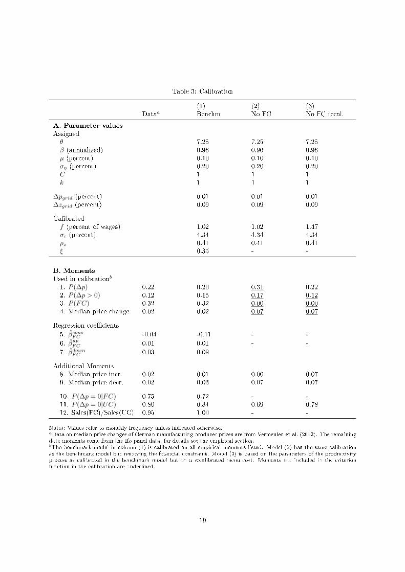
Table 3: Calibration

(1) (2) (3)Dataa Benchm No FC No FC recal.

A. Parameter valuesAssignedθ 7.25 7.25 7.25β (annualized) 0.96 0.96 0.96µ (percent) 0.10 0.10 0.10ση (percent) 0.20 0.20 0.20C 1 1 1k 1 1 1

∆pgrid (percent) 0.01 0.01 0.01∆zgrid (percent) 0.09 0.09 0.09

Calibratedf (percent of wages) 1.02 1.02 1.47σε (percent) 4.34 4.34 4.34ρz 0.41 0.41 0.41ξ 0.35 - -

B. MomentsUsed in calibrationb

1. P (∆p) 0.22 0.20 0.31 0.222. P (∆p > 0) 0.12 0.15 0.17 0.123. P (FC) 0.32 0.32 0.00 0.004. Median price change 0.02 0.02 0.07 0.07

Regression coe�cients

5. βconsFC -0.04 -0.11 - -

6. βupFC 0.01 0.01 - -

7. βdownFC 0.03 0.09 - -

Additional Moments8. Median price incr. 0.02 0.01 0.06 0.079. Median price decr. 0.02 0.03 0.07 0.07

10. P (∆p = 0|FC) 0.75 0.72 - -11. P (∆p = 0|UC) 0.80 0.84 0.69 0.7812. Sales(FC)/Sales(UC) 0.95 1.00 - -

Notes: Values refer to monthly frequency unless indicated otherwise.aData on median price changes of German manufacturing producer prices are from Vermeulen et al. (2012). The remainingdata moments come from the Ifo panel data, for details see the empirical section.bThe benchmark model in column (1) is calibrated on all empirical moments listed. Model (2) has the same calibrationas the benchmark model but removing the �nancial constraint. Model (3) is based on the parameters of the productivityprocess as calibrated in the benchmark model but on a recalibrated menu cost. Moments not included in the criterionfunction in the calibration are underlined.

19

log(z) = 0 becomes steeper,25 thus, lying closer to the price that maximizes current pro�ts. The reason

is that in this case, the �rm rationally expects to retain its current productivity level over an extended

period of time. Accordingly, possible deviations from the static pro�t maximum and the associated

payments of menu-costs are pushed further into the future and thus, become much less important than

maximizing current pro�ts.

Note that the e�ects described above break the direct link between productivity, output and being

�nancially constrained. This then explains that the dynamic benchmark model generates a ratio of sales

of constrained versus unconstrained �rms of about one which is close to the one observed in the data

(row 12 in Table 3). These e�ects become smaller (i.e. the region in which the constraint is not binding

spans a wider interval of productivity levels) when autocorrelation of productivity shocks is higher and,

hence, mean reversion is slower (see Panel (a) in Figure A-12 for policy plots whit ρz = 0.9). The

e�ects are stronger if sales are not pledgable, since the constrained optimal reset price falls even less with

increasing productivity (see Panel (b) in Figure A-12). Our benchmark model therefore replicates the

cross-sectional moments in our data in the best possible way. Tables A-16 and A-17 in the Appendix

show robustness of our calibration results to various model speci�cations.

3.3.3 The Role of Financial Frictions for the Overall Price Adjustment

In addition to our benchmark model, Table 3 exhibits the parameters and output from the model without

�nancial frictions. In the �rst version (column (2)), we keep all parameters from the benchmark and set

ξ such that the �nancial constraint never binds. Without �nancial frictions, nominal rigidities decrease,

i.e. �rms adjust their price more often (31 percent versus 20 percent in the model with frictions and the

data). They also change prices by more both upwards and downwards. We can understand these e�ects

from the price gap distributions which are displayed in Panels (c) and (d) in Figure 3. These distributions

exhibit similar di�erences between the model with and without �nancial frictions as the static model

discussed in section 3.2. As we have discussed for the static model, the smaller width of the inaction

region in the model with �nancial constraints makes every single �rm reset prices more often when

�nancially constrained. However, the distributional e�ect changes the typical position of every single

�rm in the productivity-price space when �nancial frictions are present. In particular, the price gap

distribution is less dispersed in the presence of the �nancial constraint which decreases the probability to

reset the price if menu costs stay the same. For the comparison of an economy with compared to without

�nancial frictions, the second channel dominates. Moreover, smaller inaction bounds in the presence of

�nancial frictions imply that �rms typically adjust their prices by relatively smaller amounts.

The second model without �nancial constraints keeps the productivity process constant compared

to the other model versions, but recalibrates the menu cost to match the percentage of price adjusters

in our data (column (3) in Table 3). Also in the recalibrated version of the model without �nancial

constraints, the intensive margin of price adjustment is too large compared to the respective moments

in the data. When recalibrating the model without �nancial frictions, matching the empirical price

adjustment probability of 20% means that the menu cost increases. This represents the mirror image of

the above result: The presence of �nancial frictions increases nominal rigidities.

25See Panel a) in Figure A-12 in the Appendix for the optimal price policy function for ρz = 0.9. With higher persistencethe value function is always single-peaked and there is no discrete jump in the policy function.

20

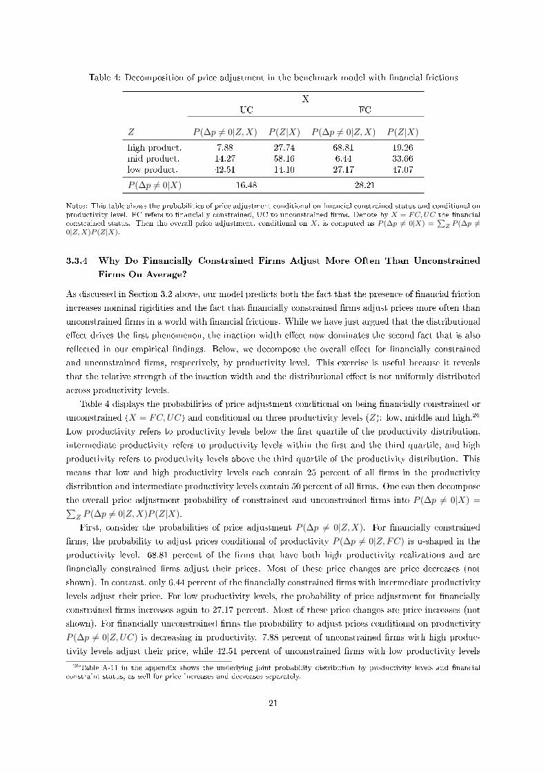
Table 4: Decomposition of price adjustment in the benchmark model with �nancial frictions

XUC FC

Z P (∆p 6= 0|Z,X) P (Z|X) P (∆p 6= 0|Z,X) P (Z|X)

high product. 7.88 27.74 68.81 19.26mid product. 14.27 58.16 6.44 33.66low product. 42.51 14.10 27.17 47.07

P (∆p 6= 0|X) 16.48 28.21

Notes: This table shows the probabilities of price adjustment conditional on �nancial constrained status and conditional onproductivity level. FC refers to �nancially constrained, UC to unconstrained �rms. Denote by X = FC,UC the �nancialconstrained status. Then the overall price adjustment, conditional on X, is computed as P (∆p 6= 0|X) =

∑Z P (∆p 6=

0|Z,X)P (Z|X).

3.3.4 Why Do Financially Constrained Firms Adjust More Often Than Unconstrained

Firms On Average?

As discussed in Section 3.2 above, our model predicts both the fact that the presence of �nancial friction

increases nominal rigidities and the fact that �nancially constrained �rms adjust prices more often than

unconstrained �rms in a world with �nancial frictions. While we have just argued that the distributional

e�ect drives the �rst phenomenon, the inaction width e�ect now dominates the second fact that is also

re�ected in our empirical �ndings. Below, we decompose the overall e�ect for �nancially constrained

and unconstrained �rms, respectively, by productivity level. This exercise is useful because it reveals

that the relative strength of the inaction width and the distributional e�ect is not uniformly distributed

across productivity levels.

Table 4 displays the probabilities of price adjustment conditional on being �nancially constrained or

unconstrained (X = FC,UC) and conditional on three productivity levels (Z): low, middle and high.26

Low productivity refers to productivity levels below the �rst quartile of the productivity distribution,

intermediate productivity refers to productivity levels within the �rst and the third quartile, and high

productivity refers to productivity levels above the third quartile of the productivity distribution. This

means that low and high productivity levels each contain 25 percent of all �rms in the productivity

distribution and intermediate productivity levels contain 50 percent of all �rms. One can then decompose

the overall price adjustment probability of constrained and unconstrained �rms into P (∆p 6= 0|X) =∑Z P (∆p 6= 0|Z,X)P (Z|X).

First, consider the probabilities of price adjustment P (∆p 6= 0|Z,X). For �nancially constrained

�rms, the probability to adjust prices conditional of productivity P (∆p 6= 0|Z,FC) is u-shaped in the

productivity level. 68.81 percent of the �rms that have both high productivity realizations and are

�nancially constrained �rms adjust their prices. Most of these price changes are price decreases (not

shown). In contrast, only 6.44 percent of the �nancially constrained �rms with intermediate productivity

levels adjust their price. For low productivity levels, the probability of price adjustment for �nancially

constrained �rms increases again to 27.17 percent. Most of these price changes are price increases (not

shown). For �nancially unconstrained �rms the probability to adjust prices conditional on productivity

P (∆p 6= 0|Z,UC) is decreasing in productivity. 7.88 percent of unconstrained �rms with high produc-

tivity levels adjust their price, while 42.51 percent of unconstrained �rms with low productivity levels

26Table A-11 in the appendix shows the underlying joint probability distribution by productivity levels and �nancialconstraint status, as well for price increases and decreases separately.

21

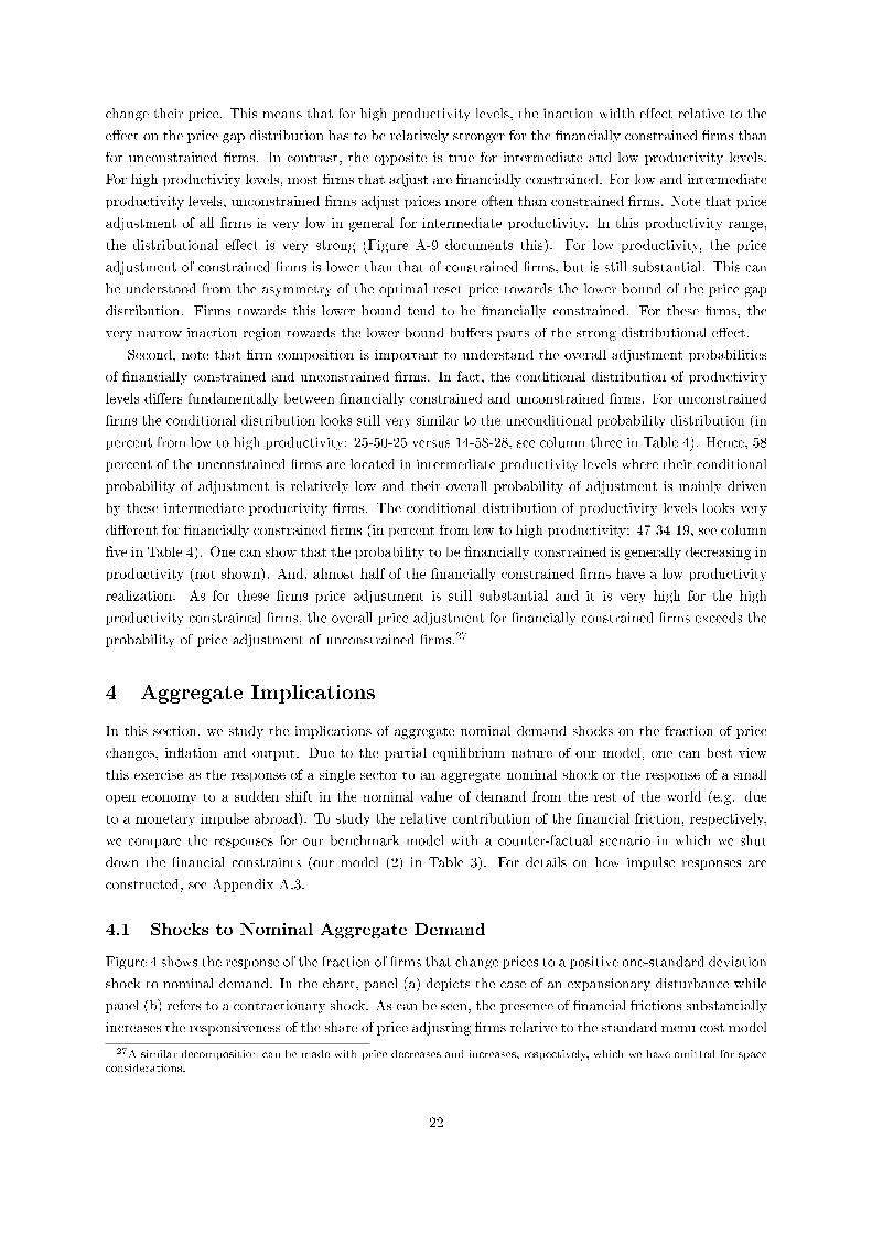
change their price. This means that for high productivity levels, the inaction width e�ect relative to the

e�ect on the price gap distribution has to be relatively stronger for the �nancially constrained �rms than

for unconstrained �rms. In contrast, the opposite is true for intermediate and low productivity levels.

For high productivity levels, most �rms that adjust are �nancially constrained. For low and intermediate

productivity levels, unconstrained �rms adjust prices more often than constrained �rms. Note that price

adjustment of all �rms is very low in general for intermediate productivity. In this productivity range,

the distributional e�ect is very strong (Figure A-9 documents this). For low productivity, the price

adjustment of constrained �rms is lower than that of constrained �rms, but is still substantial. This can

be understood from the asymmetry of the optimal reset price towards the lower bound of the price gap

distribution. Firms towards this lower bound tend to be �nancially constrained. For these �rms, the

very narrow inaction region towards the lower bound bu�ers parts of the strong distributional e�ect.

Second, note that �rm composition is important to understand the overall adjustment probabilities

of �nancially constrained and unconstrained �rms. In fact, the conditional distribution of productivity

levels di�ers fundamentally between �nancially constrained and unconstrained �rms. For unconstrained

�rms the conditional distribution looks still very similar to the unconditional probability distribution (in

percent from low to high productivity: 25-50-25 versus 14-58-28, see column three in Table 4). Hence, 58

percent of the unconstrained �rms are located in intermediate productivity levels where their conditional

probability of adjustment is relatively low and their overall probability of adjustment is mainly driven

by these intermediate productivity �rms. The conditional distribution of productivity levels looks very

di�erent for �nancially constrained �rms (in percent from low to high productivity: 47-34-19, see column

�ve in Table 4). One can show that the probability to be �nancially constrained is generally decreasing in

productivity (not shown). And, almost half of the �nancially constrained �rms have a low productivity

realization. As for these �rms price adjustment is still substantial and it is very high for the high

productivity constrained �rms, the overall price adjustment for �nancially constrained �rms exceeds the

probability of price adjustment of unconstrained �rms.27

4 Aggregate Implications

In this section, we study the implications of aggregate nominal demand shocks on the fraction of price

changes, in�ation and output. Due to the partial equilibrium nature of our model, one can best view

this exercise as the response of a single sector to an aggregate nominal shock or the response of a small

open economy to a sudden shift in the nominal value of demand from the rest of the world (e.g. due

to a monetary impulse abroad). To study the relative contribution of the �nancial friction, respectively,

we compare the responses for our benchmark model with a counter-factual scenario in which we shut

down the �nancial constraints (our model (2) in Table 3). For details on how impulse responses are

constructed, see Appendix A.3.

4.1 Shocks to Nominal Aggregate Demand

Figure 4 shows the response of the fraction of �rms that change prices to a positive one-standard deviation

shock to nominal demand. In the chart, panel (a) depicts the case of an expansionary disturbance while

panel (b) refers to a contractionary shock. As can be seen, the presence of �nancial frictions substantially

increases the responsiveness of the share of price adjusting �rms relative to the standard menu cost model

27A similar decomposition can be made with price decreases and increases, respectively, which we have omitted for spaceconsiderations.

22

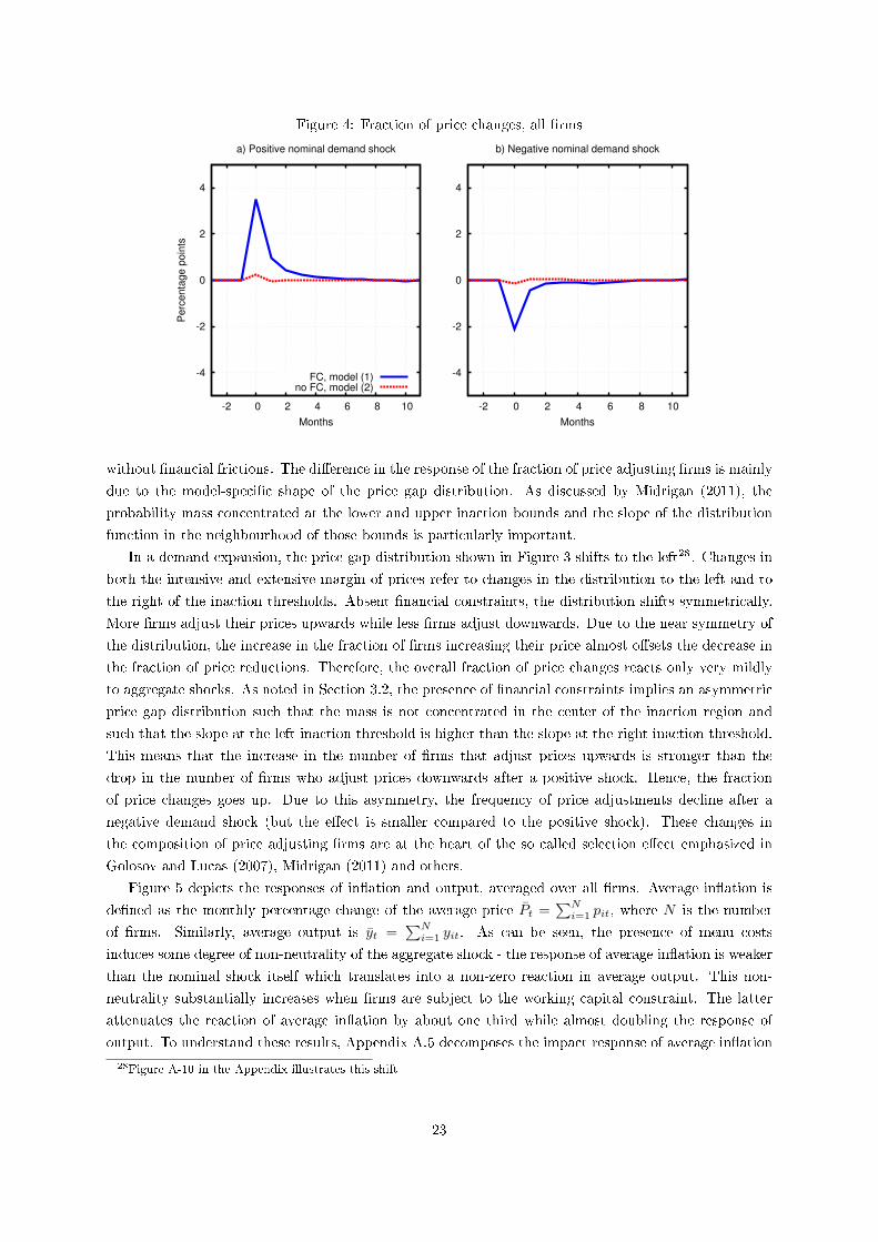
Figure 4: Fraction of price changes, all �rms

-4

-2

0

2

4

-2 0 2 4 6 8 10

Perc

enta

ge p

oin

ts

Months

a) Positive nominal demand shock

FC, model (1)no FC, model (2)

-4

-2

0

2

4

-2 0 2 4 6 8 10

Months

b) Negative nominal demand shock

without �nancial frictions. The di�erence in the response of the fraction of price adjusting �rms is mainly

due to the model-speci�c shape of the price gap distribution. As discussed by Midrigan (2011), the

probability mass concentrated at the lower and upper inaction bounds and the slope of the distribution

function in the neighbourhood of those bounds is particularly important.

In a demand expansion, the price gap distribution shown in Figure 3 shifts to the left28. Changes in

both the intensive and extensive margin of prices refer to changes in the distribution to the left and to

the right of the inaction thresholds. Absent �nancial constraints, the distribution shifts symmetrically.

More �rms adjust their prices upwards while less �rms adjust downwards. Due to the near symmetry of

the distribution, the increase in the fraction of �rms increasing their price almost o�sets the decrease in

the fraction of price reductions. Therefore, the overall fraction of price changes reacts only very mildly

to aggregate shocks. As noted in Section 3.2, the presence of �nancial constraints implies an asymmetric

price gap distribution such that the mass is not concentrated in the center of the inaction region and

such that the slope at the left inaction threshold is higher than the slope at the right inaction threshold.

This means that the increase in the number of �rms that adjust prices upwards is stronger than the

drop in the number of �rms who adjust prices downwards after a positive shock. Hence, the fraction

of price changes goes up. Due to this asymmetry, the frequency of price adjustments decline after a

negative demand shock (but the e�ect is smaller compared to the positive shock). These changes in

the composition of price adjusting �rms are at the heart of the so called selection e�ect emphasized in

Golosov and Lucas (2007), Midrigan (2011) and others.

Figure 5 depicts the responses of in�ation and output, averaged over all �rms. Average in�ation is

de�ned as the monthly percentage change of the average price Pt =∑Ni=1 pit, where N is the number

of �rms. Similarly, average output is yt =∑Ni=1 yit. As can be seen, the presence of menu costs

induces some degree of non-neutrality of the aggregate shock - the response of average in�ation is weaker

than the nominal shock itself which translates into a non-zero reaction in average output. This non-

neutrality substantially increases when �rms are subject to the working capital constraint. The latter

attenuates the reaction of average in�ation by about one third while almost doubling the response of

output. To understand these results, Appendix A.5 decomposes the impact response of average in�ation

28Figure A-10 in the Appendix illustrates this shift

23

and output into changes in the extensive and intensive margin. It is evident from that both models'

response of in�ation is almost entirely driven by the extensive margin (see Tables A-12 and A-13). In the

economy without �nancial frictions, the extensive margin of price increasers, whose number increases,

contributes almost equally strong to average in�ation as the extensive margin of price lowering �rms,

whose number declines. In our benchmark model, the contribution of the extensive margin of price

increasers is much larger as the rise in their fraction is signi�cantly stronger than the drop in the number

of price decreases as was already discussed above. The inaction regions and price gap distribution of

�rms at di�erent productivity levels are similarly a�ected by the introduction of the credit constraint29.

Thus, the behavior of the extensive margin in our benchmark model is not only driven by �rms in regions

where the maximum of the value function is associated with a binding working capital constraint, but

also by �rms for which the corresponding maximum implies a slack �nancial restriction.

However, although the fraction of price adjusters in the benchmark model exhibit a much stronger

positive reaction than the corresponding fractions in the economy without �nancial frictions, the bench-

mark model implies a weaker reaction of average in�ation. This is due to the smaller steady-state

magnitude of price changes in the benchmark economy which more than compensates the substantially

more pronounced selection e�ect compared to the model without �nancial constraints. In fact, a posi-

tive aggregate nominal demand shock reduces average price changes even further in the economy with

�nancial frictions, while it increases average price changes in the economy without �nancial frictions.

The reason is that the price gap distribution is more compressed with more mass at the lower bound of

the inaction region (see panel (d) in Figure 3). As a result of this distributional asymmetry, a large mass

of �rms increase prices by very small amounts as their prices lie only slightly below the optimal reset

price. Since many more �rms now increase prices by very little, the average price increase falls. Likewise,

the mass of �rms with small price decreases now declines, since these �rms now optimally choose not

to adjust their price. This results in an rise of the average price decrease. However, the latter e�ect is

weaker as the mass at the inaction cuto� below the optimal reset price is smaller than to above. On

the contrary, the fatter-tailed and more evenly dispersed price gap distribution in the economy without

�nancial frictions is associated with an ampli�cation of upward and an attenuation of downward price

adjustments in the case of an expansionary aggregate shock. Put di�erently, surprising changes in the

aggregate nominal price Pt are passed through to the average nominal price to a larger extent in the

economy without �nancial frictions.

Finally, to understand why the benchmark model implies a relatively stronger output reaction to

nominal aggregate shocks, note that the two models are identical regarding the economy wide demand

schedule. The latter is governed by only one parameter, the demand elasticity θ, and one exogenous

variable, the aggregate nominal price level Pt. Moreover, the �nancial friction leaves the demand side of

the economy completely una�ected. Hence, the aggregate shock shifts the demand schedule by exactly

the same amount in each of the two models. Along identical demand curves, a weaker in�ation increase

can be only associated with a more pronounced increase in output and vice versa. The implied �attening

of the supply curve means that �nancial constraints alter a central trade-o� faced by the central bank: In

order to engineer an increase in in�ation by a certain amount the monetary authority needs to generate

larger changes in nominal demand. At the same time, it needs to take into account that larger changes

in nominal demand induce even stronger responses of average real output.

29In particular, we can show that �rms with below average productivity (log(z) ∈ [−0.10,−0.03]), medium productivity(log(z) ∈ [−0.03, 0.03]) and above average productivity (log(z) ∈ [0.03, 0.1]) provide an almost equal contribution to thechange in the extensive margin. These price gap distributions are available upon request from the authors.

24

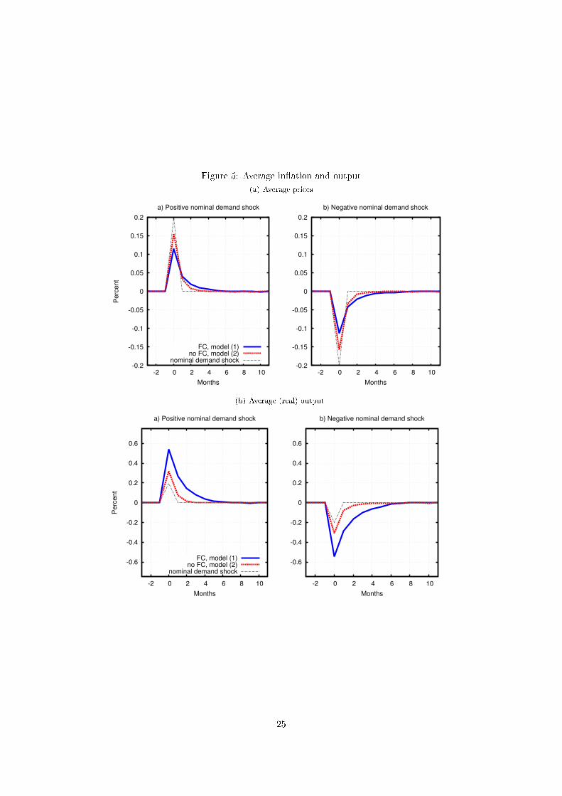
Figure 5: Average in�ation and output

(a) Average prices

-0.2

-0.15

-0.1

-0.05

0

0.05

0.1

0.15

0.2

-2 0 2 4 6 8 10

Perc

ent

Months

a) Positive nominal demand shock

FC, model (1)no FC, model (2)

nominal demand shock-0.2

-0.15

-0.1

-0.05

0

0.05

0.1

0.15

0.2

-2 0 2 4 6 8 10

Months

b) Negative nominal demand shock

(b) Average (real) output

-0.6

-0.4

-0.2

0

0.2

0.4

0.6

-2 0 2 4 6 8 10

Perc

ent

Months

a) Positive nominal demand shock

FC, model (1)no FC, model (2)

nominal demand shock

-0.6

-0.4

-0.2

0

0.2

0.4

0.6

-2 0 2 4 6 8 10

Months

b) Negative nominal demand shock

25

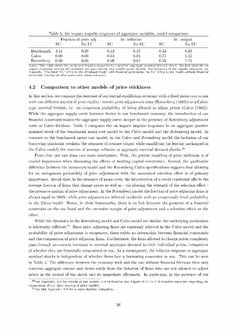
Table 5: On impact impulse responses of aggregate variables, model comparison

Fraction of price adj. Av. in�ation Av. outputFC No FC FC No FC FC No FC

Benchmark 3.41 0.23 0.12 0.15 0.53 0.33Calvo 0.00 0.00 0.04 0.04 0.71 1.15Rotemberg 0.00 0.00 0.09 0.04 0.55 1.15

Notes: This table shows the on impact impulse responses to a positive aggregate nominal demand shock. We just show the onimpact responses because the dynamics are qualitatively very similar across models. For dynamics of the impulse responses, seeAppendix. The label 'FC' refers to the simulated model with �nancial constraints, 'no FC' refers to the model without �nancialconstraint (leaving all other parameter values constant).

4.2 Comparison to other models of price stickiness

In this section, we compare the response of our partial equilibrium economy with a �xed menu cost to one

with two di�erent sources of price rigidity: convex price adjustment costs (Rotemberg (1982)) or a Calvo-

type nominal friction, i.e. an exogenous probability of being allowed to adjust prices (Calvo (1983)).

While the aggregate supply curve becomes �atter in our benchmark economy, the introduction of our

�nancial constraint makes the aggregate supply curve steeper in the presence of Rotemberg adjustment

costs or Calvo frictions. Table 5 compares the on impact impulse responses to an aggregate positive

nominal shock of the benchmark menu cost model to the Calvo model and the Rotemberg model. In

contrast to the benchmark menu cost model, in the Calvo and Rotemberg model the inclusion of our

borrowing constraint weakens the response of average output while amplifying (or leaving unchanged in

the Calvo model) the reaction of average in�ation to aggregate nominal demand shocks.30

From this, one can draw two main conclusions. First, the precise modeling of price stickiness is of

crucial importance when discussing the e�ects of working capital constraints. Second, the qualitative

di�erence between the menu-cost model and the Rotemberg/Calvo speci�cations suggests that allowing

for an endogenous probability of price adjustment with the associated selection e�ect is of primary

importance. Recall that, in the presence of menu costs, the introduction of a credit constraint a�ects the

average fraction of �rms that change prices as well as - via altering the strength of the selection e�ect -

the intensive margin of price adjustment. In the Rotemberg model the fraction of price adjusting �rms is

always equal to 100%, while price adjusters are selected randomly with an exogenously �xed probability

in the Calvo model. Hence, in these frameworks, there is no link between the presence of a �nancial

constraint on the one hand and the extensive margin of price adjustment and a selection e�ect on the

other.

While the dynamics in the Rotemberg model and Calvo model are similar, the underlying mechanism

is inherently di�erent.31 Since price adjusting �rms are randomly selected in the Calvo model and the

probability of price adjustment is exogenous, there exists no interaction between �nancial constraints

and the composition of price adjusting �rms. Furthermore, the �rms allowed to change prices completely

pass through permanent increases in nominal aggregate demand to their individual prices, irrespective

of whether they are �nancially constrained or not. As a consequence, the in�ation response to aggregate

nominal shocks is independent of whether �rms face a borrowing constraint or not. This can be seen

in Table 5. The di�erence between the economy with and the one without �nancial frictions then only

concerns aggregate output and stems solely from the behavior of �rms who are not allowed to adjust

prices in the period of the shock and its immediate aftermath. In particular, in the presence of our

30See Appendix A.6 for details of the models, the calibration and Figure A-11 for full impulse-responses regarding thecomparison of the three sources of price rigidity.

31See also Appendix A.6 for a more detailed discussion.

26

borrowing constraint, the non-adjusters that face a binding credit restriction will be forced to produce

o� their demand schedule and ration output. The fraction of such �rms tends to increase when positive

aggregate nominal shocks hit the economy and the fraction of price adjusters cannot adjust at the same

time. The opposite happens for negative demand shocks. These time varying output losses due to

rationing dampen the output response relative to a Calvo-economy without �nancial frictions.

In the case of Rotemberg adjustment costs, �rms facing a binding �nancial constraint pass changes in

the aggregate price level completely through to their individual prices. The reason is that the borrowing

restriction acts as a capacity limit. As soon as �full capacity� is reached, the �rm-speci�c supply curve is

approximately vertical and any further demand increases can only be accompanied by raising prices. In

contrast, the degree of pass-through is incomplete for unconstrained �rms. Accordingly, as long as the

fraction of �nancially constrained �rms is larger than zero, the pass-through of economy-wide nominal

demand shocks to the average price level will be stronger relative to an economy without �nancial

frictions. Consequently, the response of average output will be lower in an economy with compared to

one without �nancial frictions. To summarize, price-adjusting �rms in the Calvo model pass-through

nominal shocks completely independent of their �nancial status, but ration output when �nancially

constrained. In the Rotemberg model, no �rm rations output, but �nancially constrained �rms pass

through nominal shocks to a larger extent than unconstrained �rms, as shown in the appendix.

4.3 Robustness

We have conducted a wide variety of robustness checks for two purposes. First, to understand which

parameters/model elements are important to qualitatively and quantitatively explain the moments from

the micro data we have documented in the empirical section of this paper. Second, whether and how

the aggregate implications are a�ected by di�erent parameter values. Here we just summarize the main

�ndings. The robustness section in Appendix A.7 reports detailed tables on the calibrated parameter

values, the implied moments, the model �t to the micro data, and the implied on impact impulse responses

to an aggregate demand shock for all model versions considered here.

Myopic �rms. A model with myopic �rms (β = 0) is instructive because it shows whether considering

a dynamic model is important in order to match the micro evidence documented in the empirical section

of this paper and how important that is for the aggregate implications of the model. Both regarding

the micro moments and the aggregate implications, the model is very similar to the dynamic benchmark

model. However, the model with myopic �rms displays a lower �t to the targeted micro moments.

Regarding the pricing implications, the model with myopic �rms predicts that �nancially constrained

�rms adjust prices more often than unconstrained �rms in line with the benchmark model. However, the

myopic model model only predicts that �nancially constrained �rms adjust prices more often downwards

but not upwards. The reason was already mentioned in Section 3 above: The myopic model implies that

more productive �rms are more likely to be �nancially constrained, i.e. those �rms that have strong

incentives to decrease their prices.

Persistence of the idiosyncratic productivity shock. The persistence of the shocks are important

to explain the moments in the data, in particular the relative price adjustment frequencies of �nancially

constrained and unconstrained �rms. When the persistence of the shock is very high, the dynamic

model behaves very similar to a model with myopic �rms. That is, the slower the mean reversion,

the more important are current pro�ts relative to expected pro�ts for the optimal price decision of the

27

�rm. Ceteris paribus, higher persistence levels are associated with more price adjustment of all �rms

because with higher persistence the unconditional volatility of the idiosyncratic shock increases. For

all persistence parameters considered, �nancially constrained �rms adjust prices more often, however,

it seems that there is a non-monotonic relationship between the persistence and how much more often

�nancially constrained �rms adjust.

Model where sales are not collateralizable. With this robustness check we investigate the role of

sales as collateral. Sales as collateral are qualitatively and quantitatively important to explain the �rm

level pricing moments, in particular to explain the fact that �nancially constrained �rms adjust prices

more often upwards than unconstrained �rms. The reason is related to the discussion above. Sales in

the constraint change the elasticity of the optimal constrained reset prices with respect to idiosyncratic

shocks. And this is important in a model with forward looking �rms.

Elasticity of substitution. A crucial parameter in this model is the elasticity of substitution. We

repeat the calibration exercise for a lower and a higher demand elasticity, so that implied average mark-

ups in those alternative calibrations are 12.5 and 20 percent, respectively. The model �t does not improve

compared to the benchmark model. Furthermore, the model with lower demand elasticity generates

quantitatively too much price adjustment of �nancially constrained �rms while the model with higher

demand elasticity generates too little price adjustment of �nancially constrained �rms (in particular

upward adjusters) relative to unconstrained �rms and therefore performs less well in this respect than

the benchmark model. The aggregate implications are qualitatively similar to the benchmark model.

Idiosyncratic �nancial shocks. In the Appendix, we show a model version with both idiosyncratic

productivity and idiosyncratic �nancial shocks. For the benchmark targets, in particular targeting a

fraction of 32 percent of �nancially constrained �rms (see Table 1 section 'bank lending') this does not

improve the model �t. However, when targeting a fraction of �nancially constrained �rms that is lower

(the fraction of constrained �rms is equal to 6 percent, see section labeled 'production constrained' in

Table 1) idiosyncratic �nancial shocks help to reconcile model and the data. In particular, the model with

idiosyncratic �nancial shocks makes sure that �nancially constrained and unconstrained �rms are similar

in terms of average sales as in the data. Regarding the pricing behavior, the model performs very similar

to the benchmark model: Financially constrained �rms adjust price more often upwards and downwards.

Quantitatively, however, the model with �nancial shocks overestimate the fraction of constrained �rms

that adjust upwards and downwards and therefore the overall di�erence between �nancially constrained

and unconstrained �rms. The aggregate implications are qualitatively similar to the benchmark model.32

5 Conclusion

This paper investigates how �nancial market imperfections and nominal rigidities interact. Based on

new �rm-level evidence for Germany, we document that �nancially constrained �rms adjust prices more

often than their unconstrained counterparts, both upward and downward. We show that these empirical

patterns are consistent with a partial equilibrium menu-cost model with a working capital constraint.

Our results suggest that the presence of �nancial constraints is associated with a higher degree of nominal

rigidities, i.e. lower frequency of price changes, higher prices and lower output. Furthermore, the presence

of �nancial constraints results in a time varying frequency of price adjustments. In particular, we �nd

32The impulse responses of the model with idiosyncratic �nancial shocks are available upon request.

28

that, due to the asymmetry in the price distribution, �rms adjust prices more often in boom and less often

in a recession when �nancial constraints are present. In addition, due to the lower average frequency of

price adjustment, monetary policy shocks induce a smaller change in in�ation and a stronger reaction

of output relative to an economy without credit market imperfections. Accordingly �nancial constraints

alter a central trade-o� faced by the central bank: In order to raise in�ation by a certain amount the

monetary authority needs to accept relatively stronger responses of average output. In contrast, we

show that other sources of nominal rigidities such as exogenous probabilities of price adjustment as in

Calvo (1983) or convex price adjustment costs as in Rotemberg (1982) generate the opposite result, i.e.

the inclusion of �nancial frictions generates larger in�ation and smaller output responses to aggregate

shocks with compared to without �nancial frictions. Hence, menu costs and the associated endogenous

link between reaction of the fraction of price adjusters and the presence of �nancial imperfections are

important.

29

References

Alvarez, F. and F. Lippi (2014): �Price setting with menu cost for multiproduct �rms,� Econometrica,

82, 89�135.

Asplund, M., R. Eriksson, and N. Strand (2005): �Prices, Margins and Liquidity Constraints:

Swedish Newspapers, 1990�1992,� Economica, 72, 349�359.

Azariadis, C. and L. Kaas (2012): �Capital misallocation and aggregate factor productivity,� Working

Papers 2012-046, Federal Reserve Bank of St. Louis.

Bachmann, R., B. Born, S. Elstner, and C. Grimme (2013): �Time-Varying Business Volatility,

Price Setting, and the Real E�ects of Monetary Policy,� NBER Working Papers 19180, National

Bureau of Economic Research, Inc.

Barro, R. J. (1972): �A theory of monopolistic price adjustment,� The Review of Economic Studies,

39, 17�26.

Bhaskar, V., S. Machin, and G. C. Reid (1993): �Price and Quantity Adjustment over the Business

Cycle: Evidence from Survey Data,� Oxford Economic Papers, 45, 257�68.

Buera, F., B. Moll, and Y. Shin (2013): �Well-Intended Policies,� Review of Economic Dynamics,

16, 216�230.

Calvo, G. A. (1983): �Staggered prices in a utility-maximizing framework,� Journal of Monetary

Economics, 12, 383�398.

Caplin, A. S. and D. F. Spulber (1987): �Menu Costs and the Neutrality of Money,� The Quarterly

Journal of Economics, 102, 703�25.

Carpenter, R. E., S. M. Fazzari, and B. C. Petersen (1994): �Inventory Investment, Internal-

Finance Fluctuations, and the Business Cycle,� Brookings Papers on Economic Activity, 2, 75�138.

Chevalier, J. A. and D. S. Scharfstein (1996): �Capital market imperfections and countercyclical

markups: Theory and evidence,� American Economic Review, 86, 703�25.

Christopoulou, R. and P. Vermeulen (2012): �Markups in the Euro area and the US over the

period 1981�2004: a comparison of 50 sectors,� Empirical Economics, 42, 53�77.

Cooley, T. F. and V. Quadrini (2001): �Financial Markets and Firm Dynamics,� American Economic

Review, 91, 1286�1310.

DeutscheBundesbank (2013): �Financial accounts for Germany 2007 to 2012,� Special statistical

publication 4, Deutsche Bundesbank.

��� (2014): �Financial accounts for Germany 2008 to 2013,� Special statistical publication 4, Deutsche

Bundesbank.

Dotsey, M., R. King, and A. Wolman (1999): �State-Dependent Pricing And The General Equilib-

rium Dynamics Of Money And Output,� The Quarterly Journal of Economics, 114, 655�690.

Dotsey, M. and R. G. King (2005): �Implications of state-dependent pricing for dynamic macroeco-

nomic models,� Journal of Monetary Economics, 52, 213�242.

30

Gilchrist, S., R. Schoenle, and E. Zakrajsek (2013): �In�ation Dynamics During the Financial

Crisis,� in 2013 Meeting Papers, Society for Economic Dynamics, 826.

Golosov, M. and R. E. Lucas (2007): �Menu Costs and Phillips Curves,� Journal of Political Econ-

omy, 115, 171�199.

Gottfries, N. (1991): �Customer markets, credit market imperfections and real price rigidity,� Eco-

nomica, 58, 317�23.

��� (2002): �Market shares, �nancial constraints and pricing behaviour in the export market,� Eco-

nomica, 69, 583�607.

Guerrieri, L. and M. Iacoviello (2015): �OccBin: A toolkit for solving dynamic models with

occasionally binding constraints easily,� Journal of Monetary Economics, 70, 22�38.

Jermann, U. and V. Quadrini (2012): �Macroeconomic E�ects of Financial Shocks,� American Eco-

nomic Review, 102, 238�71.

Khan, A. and J. K. Thomas (2013): �Credit Shocks and Aggregate Fluctuations in an Economy with

Production Heterogeneity,� Journal of Political Economy, 121, 1055 � 1107.

Kimball, M. S. (1995): �The Quantitative Analytics of the Basic Neomonetarist Model,� Journal of

Money, Credit and Banking, 27, 1241�1277.

Kleemann, M. and M. Wiegand (2014): �Are Real E�ects of Credit Supply Overestimated? Bias

from Firms' Current Situation and Future Expectations,� ifo Working Paper 192, ifo institute.

Lundin, N. and L. Yun (2009): �International Trade and Inter-Industry Wage Structure in Swedish

Manufacturing: Evidence from Matched Employer�Employee Data*,� Review of International Eco-

nomics, 17, 87�102.

Midrigan, V. (2011): �Menu Costs, Multiproduct �rms, and Aggregate Fluctuations,� Econometrica,

79, 1139�1180.

Midrigan, V. and D. Y. Xu (2014): �Finance and Misallocation: Evidence from Plant-Level Data,�

American Economic Review, 104, 422�58.

Nakamura, E. and J. Steinsson (2008): �Five Facts about Prices: A Reevaluation of Menu Cost

Models,� The Quarterly Journal of Economics, 123, 1415�1464.

��� (2010): �Monetary non-neutrality in a multisector menu cost model,� The Quarterly Journal of

Economics, 125, 961�1013.

Rotemberg, J. J. (1982): �Monopolistic Price Adjustment and Aggregate Output,� Review of Economic

Studies, 49, 517�531.

Strasser, G. (2013): �Exchange rate pass-through and credit constraints,� Journal of Monetary Eco-

nomics, 60, 25�38.

Tauchen, G. (1986): �Finite state markov-chain approximations to univariate and vector autoregres-

sions,� Economics letters, 20, 177�181.

31

Vavra, J. (2013): �In�ation dynamics and time-varying uncertainty: New evidence and an ss interpre-

tation,� The Quarterly Journal of Economics, forthcoming.

Vermeulen, P., D. A. Dias, M. Dossche, E. Gautier, I. Hernando, R. Sabbatini, and

H. Stahl (2012): �Price Setting in the Euro Area: Some Stylized Facts from Individual Producer

Price Data,� Journal of Money, Credit and Banking, 44, 1631�1650.

32

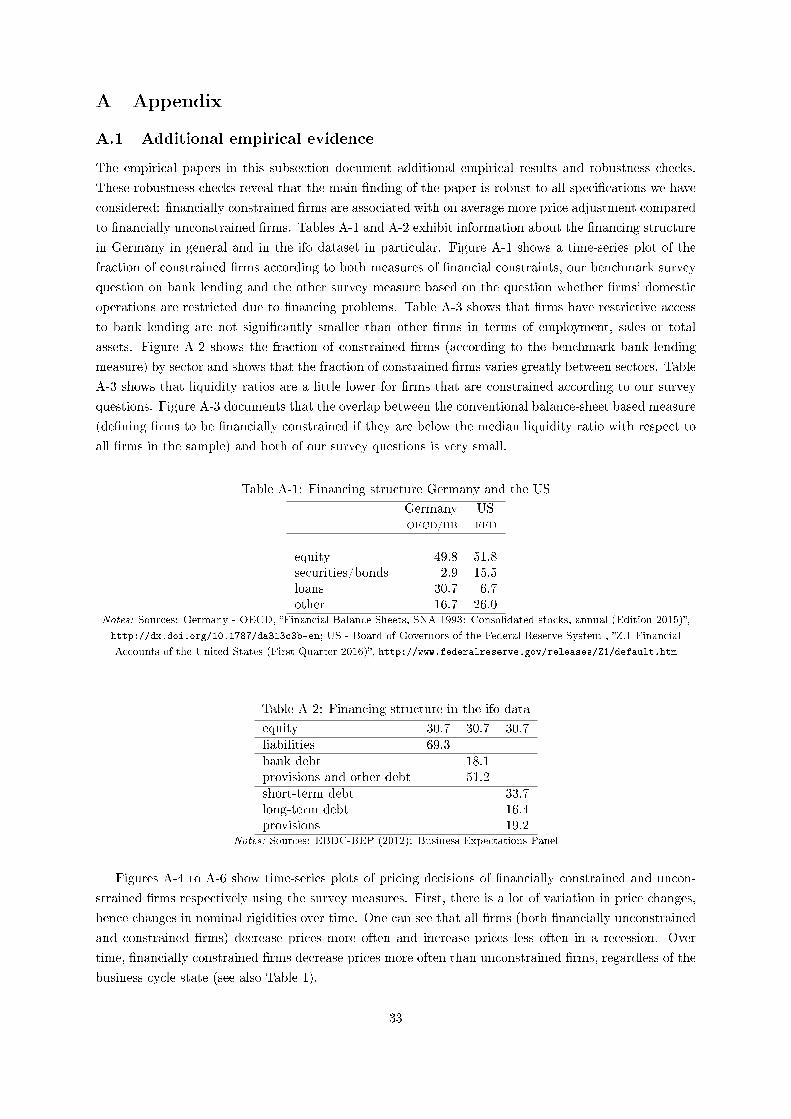
A Appendix

A.1 Additional empirical evidence

The empirical papers in this subsection document additional empirical results and robustness checks.

These robustness checks reveal that the main �nding of the paper is robust to all speci�cations we have

considered: �nancially constrained �rms are associated with on average more price adjustment compared

to �nancially unconstrained �rms. Tables A-1 and A-2 exhibit information about the �nancing structure

in Germany in general and in the ifo dataset in particular. Figure A-1 shows a time-series plot of the

fraction of constrained �rms according to both measures of �nancial constraints, our benchmark survey

question on bank lending and the other survey measure based on the question whether �rms' domestic

operations are restricted due to �nancing problems. Table A-3 shows that �rms have restrictive access

to bank lending are not signi�cantly smaller than other �rms in terms of employment, sales or total

assets. Figure A-2 shows the fraction of constrained �rms (according to the benchmark bank lending

measure) by sector and shows that the fraction of constrained �rms varies greatly between sectors. Table

A-3 shows that liquidity ratios are a little lower for �rms that are constrained according to our survey

questions. Figure A-3 documents that the overlap between the conventional balance-sheet based measure

(de�ning �rms to be �nancially constrained if they are below the median liquidity ratio with respect to

all �rms in the sample) and both of our survey questions is very small.

Table A-1: Financing structure Germany and the US

Germany USOECD/BB FED

equity 49.8 51.8securities/bonds 2.9 15.5loans 30.7 6.7other 16.7 26.0

Notes: Sources: Germany - OECD, �Financial Balance Sheets, SNA 1993: Consolidated stocks, annual (Edition 2015)�,

http://dx.doi.org/10.1787/da313c3b-en; US - Board of Governors of the Federal Reserve System , �Z.1 Financial

Accounts of the United States (First Quarter 2016)�, http://www.federalreserve.gov/releases/Z1/default.htm

Table A-2: Financing structure in the ifo data

equity 30.7 30.7 30.7liabilities 69.3bank debt 18.1provisions and other debt 51.2short-term debt 33.7long-term debt 16.4provisions 19.2

Notes: Sources: EBDC-BEP (2012): Business Expectations Panel

Figures A-4 to A-6 show time-series plots of pricing decisions of �nancially constrained and uncon-

strained �rms respectively using the survey measures. First, there is a lot of variation in price changes,

hence changes in nominal rigidities over time. One can see that all �rms (both �nancially unconstrained

and constrained �rms) decrease prices more often and increase prices less often in a recession. Over

time, �nancially constrained �rms decrease prices more often than unconstrained �rms, regardless of the

business cycle state (see also Table 1).

33

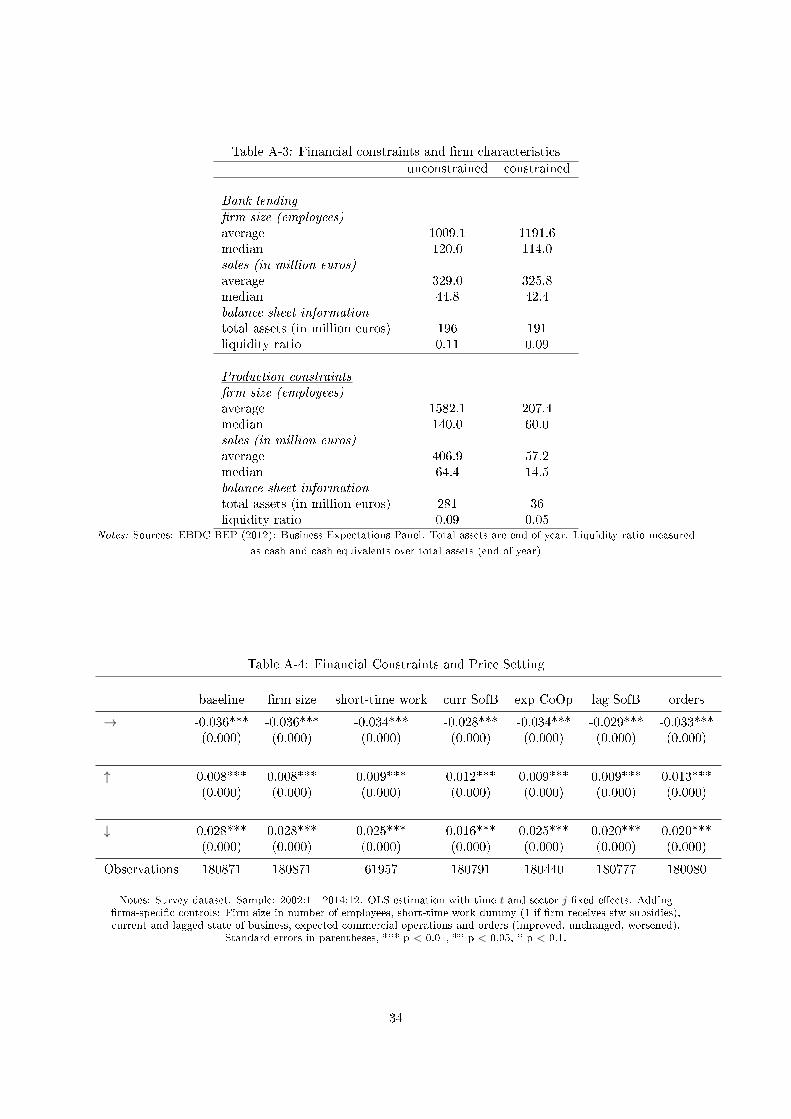
Table A-3: Financial constraints and �rm characteristics

unconstrained constrained

Bank lending

�rm size (employees)average 1009.1 1191.6median 120.0 114.0sales (in million euros)average 329.0 325.8median 44.8 42.4balance sheet informationtotal assets (in million euros) 196 191liquidity ratio 0.11 0.09

Production constraints�rm size (employees)average 1582.1 207.4median 140.0 60.0sales (in million euros)average 406.9 57.2median 64.4 14.5balance sheet informationtotal assets (in million euros) 281 36liquidity ratio 0.09 0.05

Notes: Sources: EBDC-BEP (2012): Business Expectations Panel. Total assets are end of year. Liquidity ratio measured

as cash and cash equivalents over total assets (end of year)

Table A-4: Financial Constraints and Price Setting

baseline �rm size short-time work curr SofB exp CoOp lag SofB orders

→ -0.036*** -0.036*** -0.034*** -0.028*** -0.034*** -0.029*** -0.033***(0.000) (0.000) (0.000) (0.000) (0.000) (0.000) (0.000)

↑ 0.008*** 0.008*** 0.009*** 0.012*** 0.009*** 0.009*** 0.013***(0.000) (0.000) (0.000) (0.000) (0.000) (0.000) (0.000)

↓ 0.028*** 0.028*** 0.025*** 0.016*** 0.025*** 0.020*** 0.020***(0.000) (0.000) (0.000) (0.000) (0.000) (0.000) (0.000)

Observations 180871 180871 61957 180791 180440 180777 180080

Notes: Survey dataset. Sample: 2002:1 - 2014:12. OLS estimation with time t and sector j �xed e�ects. Adding�rms-speci�c controls: Firm size in number of employees, short-time work dummy (1 if �rm receives stw subsidies),current and lagged state of business, expected commercial operations and orders (improved, unchanged, worsened).

Standard errors in parentheses, *** p < 0.01, ** p < 0.05, * p < 0.1.

34

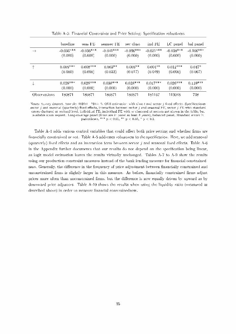
Table A-5: Financial Constraints and Price Setting: Speci�cation robustness

baseline seas FE seassec FE sec clust ind FE LC panel bal panel

→ -0.036*** -0.036*** -0.041*** -0.036*** -0.021*** -0.038*** -0.166***(0.000) (0.000) (0.000) (0.000) (0.000) (0.000) (0.000)

↑ 0.008*** 0.008*** 0.003** 0.008** 0.004** 0.012*** 0.047*(0.000) (0.000) (0.033) (0.017) (0.049) (0.000) (0.067)

↓ 0.028*** 0.028*** 0.038*** 0.028*** 0.017*** 0.026*** 0.119***(0.000) (0.000) (0.000) (0.000) (0.000) (0.000) (0.000)

Observations 180871 180871 180871 180871 181167 113048 728

Notes: Survey dataset. Sample: 2002:1 - 2014:12. OLS estimation with time t and sector j �xed e�ects. Speci�cations:sector j and seasonal (quarterly) �xed e�ects, interaction between sector j and seasonal FE, sector j FE with standarderrors clustered at sectoral level, individual FE, individual FE with se clustered at sectors not shown in the table, butavailable upon request. Long-coverage panel (�rms are in panel at least 8 years), balanced panel. Standard errors in

parentheses, *** p < 0.01, ** p < 0.05, * p < 0.1.

Table A-4 adds various control variables that could a�ect both price setting and whether �rms are

�nancially constrained or not. Table A-5 addresses robustness to the speci�cation. Here, we add seasonal

(quarterly) �xed e�ects and an interaction term between sector j and seasonal �xed e�ects. Table A-6

in the Appendix further documents that our results do not depend on the speci�cation being linear,

as logit model estimation leaves the results virtually unchanged. Tables A-7 to A-9 show the results

using our production constraint measures instead of the bank lending measure for �nancial constrained-

ness. Generally, the di�erence in the frequency of price adjustment between �nancially constrained and

unconstrained �rms is slightly larger in this measure. As before, �nancially constrained �rms adjust

prices more often than unconstrained �rms, but the di�erence is now equally driven by upward as by

downward price adjusters. Table A-10 shows the results when using the liquidity ratio (measured as

described above) in order to measure �nancial constrainedness.

35

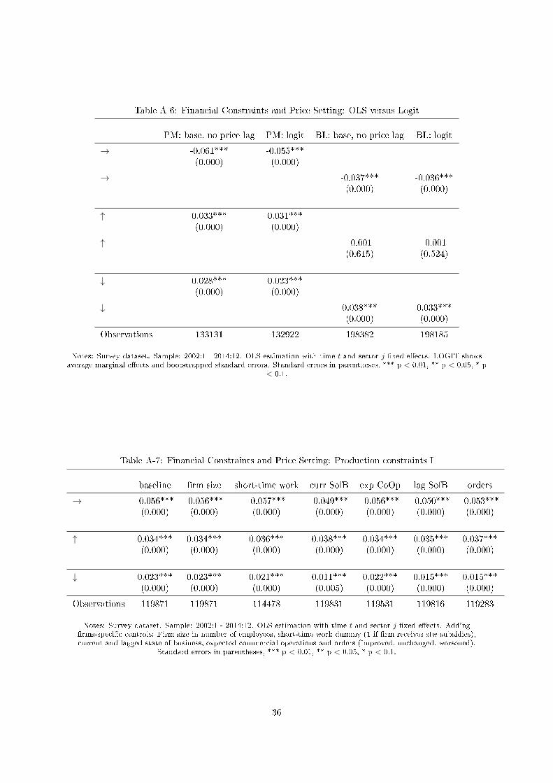
Table A-6: Financial Constraints and Price Setting: OLS versus Logit

PM: base, no price lag PM: logit BL: base, no price lag BL: logit

→ -0.061*** -0.055***(0.000) (0.000)

→ -0.037*** -0.036***(0.000) (0.000)

↑ 0.033*** 0.031***(0.000) (0.000)

↑ -0.001 -0.001(0.615) (0.524)

↓ 0.028*** 0.023***(0.000) (0.000)

↓ 0.038*** 0.033***(0.000) (0.000)

Observations 133131 132922 198382 198185

Notes: Survey dataset. Sample: 2002:1 - 2014:12. OLS estimation with time t and sector j �xed e�ects. LOGIT showsaverage marginal e�ects and bootstrapped standard errors. Standard errors in parentheses, *** p < 0.01, ** p < 0.05, * p

< 0.1.

Table A-7: Financial Constraints and Price Setting: Production constraints I

baseline �rm size short-time work curr SofB exp CoOp lag SofB orders

→ -0.056*** -0.056*** -0.057*** -0.049*** -0.056*** -0.050*** -0.053***(0.000) (0.000) (0.000) (0.000) (0.000) (0.000) (0.000)

↑ 0.034*** 0.034*** 0.036*** 0.038*** 0.034*** 0.035*** 0.037***(0.000) (0.000) (0.000) (0.000) (0.000) (0.000) (0.000)

↓ 0.023*** 0.023*** 0.021*** 0.011*** 0.022*** 0.015*** 0.015***(0.000) (0.000) (0.000) (0.005) (0.000) (0.000) (0.000)

Observations 119871 119871 114478 119831 119531 119816 119283

Notes: Survey dataset. Sample: 2002:1 - 2014:12. OLS estimation with time t and sector j �xed e�ects. Adding�rms-speci�c controls: Firm size in number of employees, short-time work dummy (1 if �rm receives stw subsidies),current and lagged state of business, expected commercial operations and orders (improved, unchanged, worsened).

Standard errors in parentheses, *** p < 0.01, ** p < 0.05, * p < 0.1.

36

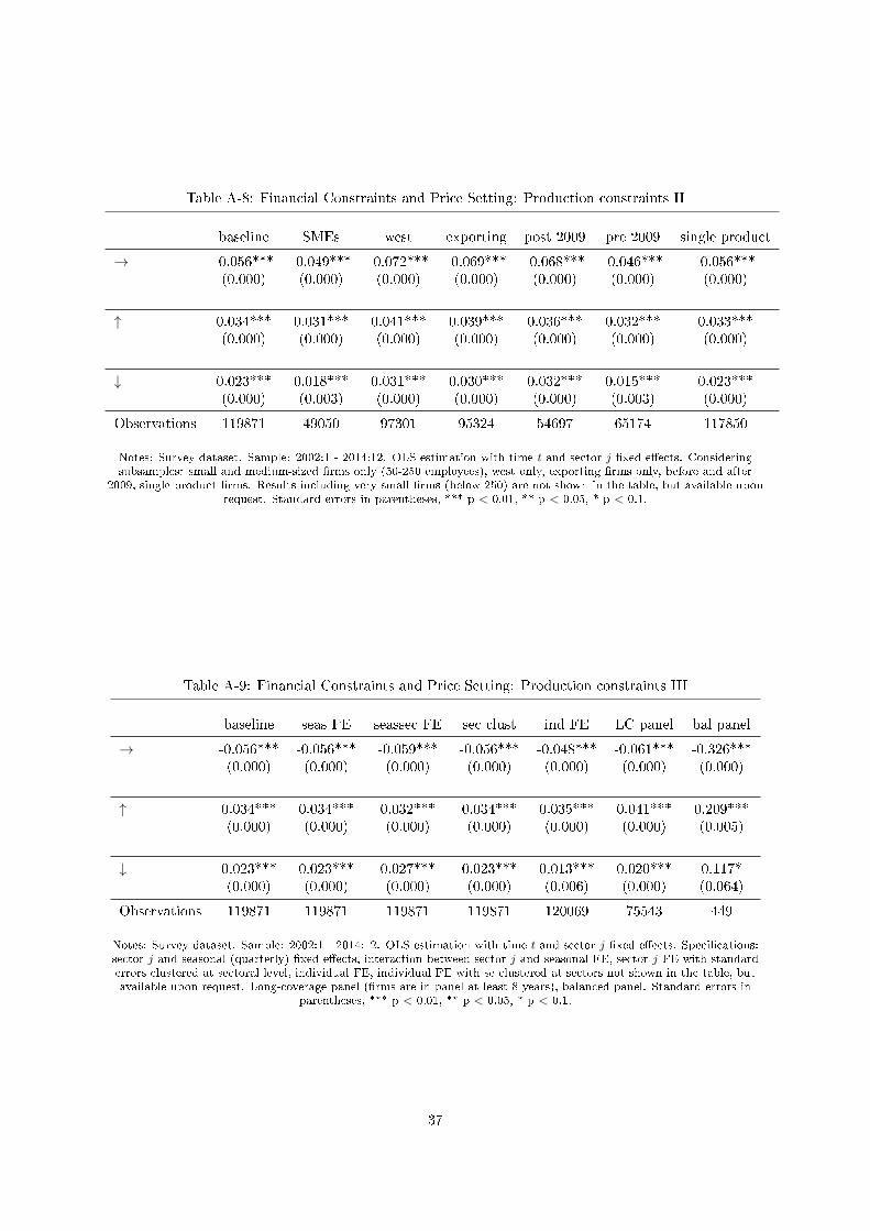
Table A-8: Financial Constraints and Price Setting: Production constraints II

baseline SMEs west exporting post 2009 pre 2009 single product

→ -0.056*** -0.049*** -0.072*** -0.069*** -0.068*** -0.046*** -0.056***(0.000) (0.000) (0.000) (0.000) (0.000) (0.000) (0.000)

↑ 0.034*** 0.031*** 0.041*** 0.039*** 0.036*** 0.032*** 0.033***(0.000) (0.000) (0.000) (0.000) (0.000) (0.000) (0.000)

↓ 0.023*** 0.018*** 0.031*** 0.030*** 0.032*** 0.015*** 0.023***(0.000) (0.003) (0.000) (0.000) (0.000) (0.003) (0.000)

Observations 119871 49050 97301 95324 54697 65174 117850

Notes: Survey dataset. Sample: 2002:1 - 2014:12. OLS estimation with time t and sector j �xed e�ects. Consideringsubsamples: small and medium-sized �rms only (50-250 employees), west only, exporting �rms only, before and after

2009, single product �rms. Results including very small �rms (below 250) are not shown in the table, but available uponrequest. Standard errors in parentheses, *** p < 0.01, ** p < 0.05, * p < 0.1.

Table A-9: Financial Constraints and Price Setting: Production constraints III

baseline seas FE seassec FE sec clust ind FE LC panel bal panel

→ -0.056*** -0.056*** -0.059*** -0.056*** -0.048*** -0.061*** -0.326***(0.000) (0.000) (0.000) (0.000) (0.000) (0.000) (0.000)

↑ 0.034*** 0.034*** 0.032*** 0.034*** 0.035*** 0.041*** 0.209***(0.000) (0.000) (0.000) (0.000) (0.000) (0.000) (0.005)

↓ 0.023*** 0.023*** 0.027*** 0.023*** 0.013*** 0.020*** 0.117*(0.000) (0.000) (0.000) (0.000) (0.006) (0.000) (0.064)

Observations 119871 119871 119871 119871 120069 75543 449

Notes: Survey dataset. Sample: 2002:1 - 2014:12. OLS estimation with time t and sector j �xed e�ects. Speci�cations:sector j and seasonal (quarterly) �xed e�ects, interaction between sector j and seasonal FE, sector j FE with standarderrors clustered at sectoral level, individual FE, individual FE with se clustered at sectors not shown in the table, butavailable upon request. Long-coverage panel (�rms are in panel at least 8 years), balanced panel. Standard errors in

parentheses, *** p < 0.01, ** p < 0.05, * p < 0.1.

37

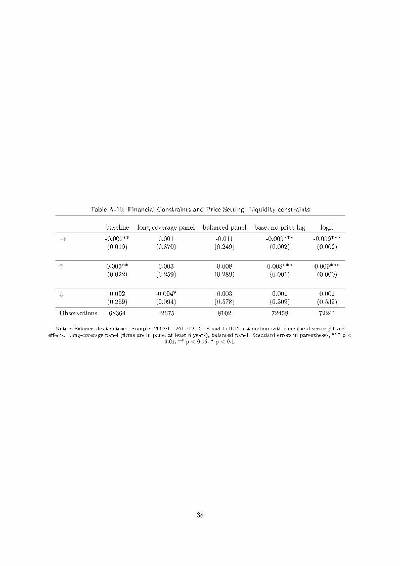
Table A-10: Financial Constraints and Price Setting: Liquidity constraints

baseline long coverage panel balanced panel base, no price lag logit

→ -0.007** 0.001 -0.011 -0.009*** -0.009***(0.019) (0.870) (0.249) (0.002) (0.002)

↑ 0.005** 0.003 0.008 0.008*** 0.009***(0.022) (0.259) (0.289) (0.001) (0.000)

↓ 0.002 -0.004* 0.003 0.001 0.001(0.269) (0.094) (0.578) (0.509) (0.535)

Observations 68364 42675 8102 72458 72241

Notes: Balance sheet dataset. Sample: 2002:1 - 2011:12. OLS and LOGIT estimation with time t and sector j �xede�ects. Long-coverage panel (�rms are in panel at least 8 years), balanced panel. Standard errors in parentheses, *** p <

0.01, ** p < 0.05, * p < 0.1.

38

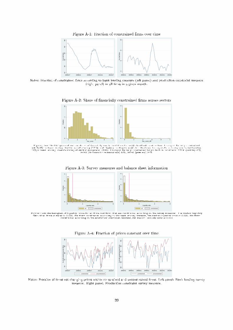
Figure A-1: Fraction of constrained �rms over time

1020

3040

5060

% o

f all

firm

s

2003m7 2006m1 2008m7 2011m1 2013m7

46

810

% o

f all

firm

s

2002m1 2004m1 2006m1 2008m1 2010m1 2012m1 2014m1

Notes: Fraction of constrained �rms according to bank lending measure (left panel) and production constraint measure(right panel) in all �rms in a given month.

Figure A-2: Share of �nancially constrained �rms across sectors

0.0

5.1

.15

Fra

ctio

n

0 .2 .4 .6 .8 1frac_const

0.2

.4.6

Fra

ctio

n

0 .2 .4 .6 .8 1frac_const_diff

Figures show the histogram of various shares of �nancially constrained �rms for wz93 classi�cation of sectors. Examples for very constrained(90-100%) in bank lending: textile manufacturing (17150 and 17300 according to wz93 classi�cation). Examples for not very constrained (below10%)in bank lending: manufacturing of electric equipment, 31600. Examples for very constrained for production constraint: 17300 (textile) 22%,

26240 (ceramics for technical use) 33%, 36200 (jewelery) 34%.

Figure A-3: Survey measures and balance sheet information

0.1

.2.3

.4F

ract

ion

0 .1 .2 .3Liquidity ratio

all constrained

0.1

.2.3

.4.5

Fra

ctio

n

0 .1 .2 .3Liquidity ratio

all constrained

Figures show the histogram of liquidity ratios for all �rms and �rms that are constrained according to the survey measures. The median liquidityratio of all �rms is equal to 0.036. For �rms constrained according to the bank lending measure, the median liquidity ratio is 0.026. For �rms

constrained according to the production constraint measure, the median liquidity ratio is 0.014

Figure A-4: Fraction of prices constant over time

7075

8085

90%

of a

ll co

nstr

/unc

onst

r fir

ms

2003m7 2006m1 2008m7 2011m1 2013m7

constrained unconstrained

6065

7075

8085

% o

f all

cons

tr/u

ncon

str

firm

s

2002m1 2004m1 2006m1 2008m1 2010m1 2012m1 2014m1

constrained unconstrained

Notes: Fraction of �rms not changing prices within constrained and unconstrained �rms. Left panel: Bank lending surveymeasure. Right panel: Production constraint survey measure.

39

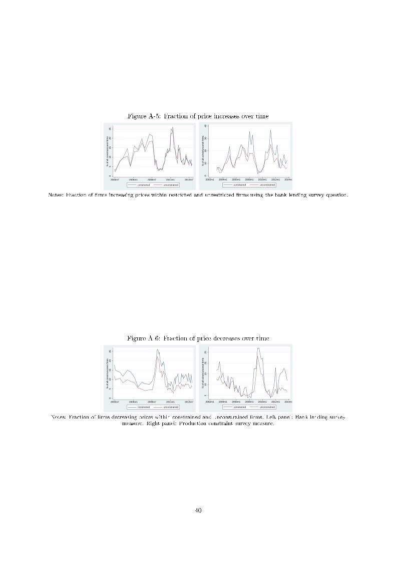
Figure A-5: Fraction of price increases over time0

510

1520

25%

of a

ll co

nstr

/unc

onst

r fir

ms

2003m7 2006m1 2008m7 2011m1 2013m7

constrained unconstrained

010

2030

40%

of a

ll co

nstr

/unc

onst

r fir

ms

2002m1 2004m1 2006m1 2008m1 2010m1 2012m1 2014m1

constrained unconstrained

Notes: Fraction of �rms increasing prices within restricted and unrestricted �rms using the bank lending survey question.

Figure A-6: Fraction of price decreases over time

05

1015

2025

% o

f all

cons

tr/u

ncon

str

firm

s

2003m7 2006m1 2008m7 2011m1 2013m7

constrained unconstrained

510

1520

25%

of a

ll co

nstr

/unc

onst

r fir

ms

2002m1 2004m1 2006m1 2008m1 2010m1 2012m1 2014m1

constrained unconstrained

Notes: Fraction of �rms decreasing prices within constrained and unconstrained �rms. Left panel: Bank lending surveymeasure. Right panel: Production constraint survey measure.

40

A.2 The model with myopic �rms

The purpose of this subsection is threefold. First, we provide the formal proofs to the claims in the main

text for the simpli�ed model with β = 0. Second, we show that there is no unambiguous relationship

between �rm productivity and a binding �nancial constraint. In fact, this depends crucially on whether

the �rm decides to adjust the price or not; in case of no price adjustment, low productivity �rms are more

likely to be �nancially constrained, while in the case of price adjustment, �rms with relatively higher

productivity will be more likely �nancially constrained. Third, we show that �nancially constrained �rms

that optimally adjust the price charge a mark-up over marginal costs that is increasing in productivity.

This implies that �nancially constrained �rms, on average, have higher mark-ups.

A.2.1 Problem of the �rm

For simplicity, we normalize the aggregate price level P = 1. Hence, the �rm's nominal price is also

its real price. To save on notation, we drop all time indices. In addition, we normalize the aggregate

consumption level C = 1. Also recall that we have normalized real wages by w = (θ−1)/θ. The problem

of the �rm can then be written as

V (p, z) = max{V a(p, z), V na(p, z)}

where the value of price adjustment is given by

V A(p, z) = maxh,q 6=p

{zh

(q − w

z

)− fw

}

subject to

zh ≤ q−θ (φ)

wh ≤ ξ(1 + qzh) (µ)

and the value of not adjusting the price is given by

V NA(p, s) = maxh

zh

(p− w

z

)

subject to

zh ≤ p−θ (φ)

wh ≤ ξ(1 + pzh) (µ)

where as in the main text we have normalized capital, ki = 1 for all i.

41

A.2.2 No price adjustment

Conditional on not adjusting the price, the �rm chooses hours to maximize pro�ts. The �rst order

conditions read as

0 =

(p− w

z

)− φ+ µ

(ξp− w

z

)zh ≤ p−θ ⊥ φ ≥ 0

wh ≤ ξ(1 + pzh) ⊥ µ ≥ 0

For z ≤ w/p the optimal solution is h = y = φ = µ = 0. That is, for a given price, �rms with su�ciently

low productivity do not produce. In what follows assume pz > w and consider the following cases:

1. Demand holds with equality while the �nancial constraint is slack. Complementary slackness

requires µ = 0. From the demand equation we have

h =1

zp−θ

φ =

(p− w

z

)Note that in this case it has to be true that

z >w

ξ(pθ + p)(A.1)

that is, �rms with su�ciently high productivity (given the price) are unconstrained. Notice that

this condition only gets some bite if we further assume that wξ(pθ+p)

> w/p or ξ < ppθ+p

at least for

some p. Otherwise, (A.1) would be always the trivially satis�ed for all �rms (recall by assumption

pz > w).

2. Demand is slack while the �nancial constraint is binding. Complementary slackness requires φ = 0.

Then we have

h =ξ

w − ξpz

µ =pz − ww − ξpz

(A.2)

This solution assumes that φ = 0. This is the case whenever z ≤ wξ(pθ+p)

which is just the

complement of the requirement in case 1 above. Notice that when this condition is met, it is

also true that z < wpξ which is the requirement for µ ≥ 0. This means that for given p and ξ,

�rms productivity below this threshold are constrained. Furthermore, inspecting equation (A.2)

reveals that for a given price, the Lagrange multiplier µ is increasing in productivity z. This is

intuitive because for higher productivity �rms the shadow value of relaxing the �nancial constraint

marginally is higher than for �rms with relatively less productivity (more precisely the gradient

of the Lagrange function increases for higher productivity because the pro�t function is increasing

in z). However, once productivity is high enough the �rm needs so little labor input to satisfy

the demand at the current price that the �nancial constraint is no longer binding. The Lagrange

multiplier then falls to zero.

To summarize, it is worth highlighting that conditional on not adjusting the price, the �rms with low

42

productivity are �nancially constrained. On the other hand, �rms with su�ciently high productivity

above a certain threshold are �nancially unconstrained.

A.2.3 Price adjustment

In case the �rm chooses to adjust the price optimally, i.e. conditional on paying the �x cost, the �rst

order conditions for prices, hours, and output are given by

0 = zh+ µξzh− φθq−θ−1

0 =

(q − w

z

)− φ− µ

(wz− ξp

)zh ≤ q−θ ⊥ φ ≥ 0

wh ≤ ξ(1 + pzh) ⊥ µ ≥ 0

Consider the following cases:

1. The �nancial constraint is binding and the demand function is slack. In this case, by hypothesis

φ = 0 and

h =ξ

w − ξqz0 = zh(1 + ξµ)

µ =(wz− ξq

)−1((

q − w

z

)).

This implies h = 0, a contradiction unless ξ = 0, assuming that productivity is always positive

z > 0 and focusing on positive prices q > 0 (which is without loss of generality as demand is in�nite

for a zero price). Henceforth, we exclude this case by assuming that ξ > 0. Therefore, in case the

�rm �nds it optimal to adjust its price, it will always satisfy demand.

2. The �nancial constraint is not binding and demand is satis�ed. This implies that µ = 0 and

h =1

zq−θ

0 = zh− φθq−θ−1

φ =

(q − w

z

)

so that

0 = 1− θ(q − w

z

)q−1

or

q =θ

θ − 1

w

z(A.3)

which is the familiar result that optimal price is a constant mark-up θ/(θ− 1) over marginal costs

w/z.

43

3. Both, the demand function and the �nancial constraint are satis�ed with equality. Then

h =ξ

w − ξqzq−θ = zh

φ =1

θzhq1+θ(1 + ξµ)

µ =(wz− ξq

)−1((

q − w

z

)− φ

). (A.4)

Hence, the price of the constrained �rm solves

q−θ =ξz

w − ξqz(A.5)

Alternatively, as in the main text, the optimal constrained adjusting price can be expressed in

terms of the Lagrange multiplier that is attached to the �nancial constraint:

q =(1 + µ)

(1 + µξ)

θ

θ − 1

w

z

where the Lagrange multiplier µ solves equation (A.4). Notice that in principle equation (A.5)

can have multiple and complex solutions. However, as this equation is a polynomial of degree θ

with only one sign change, there is at most one positive solution.33 So any other (complex or real)

solutions to equation (A.5) are non-positive. We can exclude solutions involving negative prices

because in that case the Lagrange multiplier µ is negative, clearly a contradiction. Henceforth, we

focus on positive real solutions to equation (A.5).34 It is straightforward to show that the solution

to equation (A.5) that is consistent with a positive Lagrange multiplier µ ≥ 0 lies in the interval

q ∈ [ 1z ,

1ξz ) if and only if ξ < 1.35 With other words, ξ < 1 is a necessary and su�cient condition

for the existence of a unique positive solution to equations (A.5) that is consistent with a positive

Lagrange-multiplier.

We now are ready to show that the Lagrange multiplier µ is increasing in productivity. First, we

use a change of variables x = qz and rewrite (A.4) as µ(1− ξx) = (x− 1). Notice that x ∈ [1, 1/ξ)

whenever ξ < 1 (see above). Taking the total derivative and rearranging we obtain

dµ =1 + ξµ

1− ξxdx, (A.6)

33To see this, rewrite (A.5) as ξ(qθ + q)− w/z = 0.34For θ = 2 we can solve for the price analytically and show that there are two real solutions, one negative and one

positive. Abstracting from the negative solution (as this would imply a negative Lagrange multiplier), the optimal adjusting

price is given by q = 0.5(√

(1 + 4w/(ξz))− 1) which is strictly positive for any w, ξ, z > 0. In addition, at this price hoursworked are positive (h > 0) for any w, ξ, z > 0.

35Suppose ξ < 1. First we show that qz < 1/ξ so that the inverse term on the right hand side of equation (A.4) is wellde�ned and strictly positive. Combine equations (A.4) and (A.5) and use the normalization of wages w = (θ− 1)/θ to get

qz <1

ξ⇔

(1 + µ)

(1 + µξ)<

1

ξ⇔ ξ < 1

where we have used the fact that µ ≥ 0 by assumption. Second, we show that qz ≥ 1. Use the normalization of wages andrewrite equation (A.4) as

µ =

(1

z− ξq

)−1 (q −

1

z

)The �rst inverse term is strictly positive for ξ < 1 as shown above. This implies that µ ≥ requires q ≥ 1/z.

44

which says that the Lagrange multiplier is increasing in x for ξ < 1. Using the same change of

variables and taking the total derivative of equation (A.5) we obtain the result that x is increasing

in z:

dx = ξx

1− ξx

(xz

)θdz (A.7)

Recall that θ > 1 and x ∈ [1, 1/ξ) for ξ < 1, so that the right side is positive for positive

changes in z. This means that x = pz � the revenue per unit labor employed � is increasing in

productivity. Finally, combining (A.6) and (A.7) gives the result that the Lagrange multiplier

is increasing in productivity. With other words, the mark-up of �nancially constrained �rms is

monotonically increasing in productivity because the mark-up depends on the Lagrange multiplier

which is increasing in productivity.

Finally, together with the result that the mark-up of unconstrained price adjusting �rms is constant

(see equation (A.3)), this implies that there is a productivity cut-o� for which the �rms become

�nancially constrained: only �rms with su�ciently high productivity z ≥ z are �nancially con-

strained. One can solve for the threshold productivity z by equating the unconstrained price with

the �nancially constrained price and then using (A.5) to solve for productivity. Formally, �rms are

�nancially constrained if and only if

z ≥(

ξ

w − ξ

) 1θ−1

and unconstrained otherwise (case 2. above). Notice that this threshold productivity is strictly

positive if and only if ξ < w where by normalization w < 1. In all calibrations in the main text we

assume that ξ < w.36

The last remark concerns the pass-through of idiosyncratic shocks: the optimal price of �nancially

constrained �rms responds less to productivity shocks than the price of adjusting unconstrained

�rms. To see this, note that equation (A.3) implies that revenue per unit labor xuc = qucz does not

change when productivity changes, or formally dxuc = dz = 0; this is only possible if unconstrained

optimal prices decrease (increase) one for one with positive (negative) productivity shocks. On the

other hand, in equation (A.7), we have shown that for constrained �rms dxfc = dz > 0. This means

the constrained price qfc changes less than one for one with productivity shocks, or |dqfc| < |dz|.With other words, for �nancially constrained �rms, there is incomplete pass-through of idiosyncratic

shocks. This result is key for understanding the stationary price distribution and the transmission

of aggregate nominal shocks. We provide more intuition in the following subsection.

A.2.4 Summary and intuition

In case the �rm does not adjust the price, for example because the menu cost is large, condition (A.1)

tells us that �rms with su�ciently low productivity levels are �nancially constrained. The intuition

behind this result is the following. For low productivity levels, �rms need a relatively large amount of

labor input in order to produce the amount that is demanded at the given price. For those �rms the wage

bill that has to be �nanced is relatively high and it is therefore more likely that those low productivity

�rms face a binding constraint. Once productivity increases, the required labor input decreases, the wage

36To be more precise, for all calibrations the guess of ξ for the numerical solver is set to a value below w. In all simulationsand all iterations, the numerical solver always selected lower values of ξ and never considered selected values close or abovew.

45

bill that has to be �nanced decreases, and this relaxes the �nancial constraint. If productivity is large

enough the constraint becomes eventually non-binding.

In case of price adjustment, �rms with higher productivity levels are likely to be more constrained.

This is an implication from the fact that the Lagrange multiplier is increasing in productivity z, as shown

analytically above. As mentioned above, for �rms with higher productivity, the optimal constrained price

lies further away from the optimal unconstrained price (the latter exhibiting a constant markup). The

reason for the positive relationship between µ and z can be understood by noting that the Lagrangean

multiplier µ measures the marginal rise in pro�ts resulting from an in�nitesimal loosening of a binding

�nancial constraint. To see this, recall that when both, the �nancial and the demand constraint bind,

the �rst derivative of �rm i's Lagrange function with respect to the individual nominal price pi imply

µi =∂Πi

∂pi︸︷︷︸A

·

B︷ ︸︸ ︷(1

wz∂Di∂pi

),

where Πi and Di denote �rm i' pro�ts and demand respectively. Note further, that the term in brackets

B equals the amount of the nominal price decrease which becomes possible due to an in�nitesimal

loosening of the credit constraint. The term A measures the change in pro�ts induced by an unit

in�nitesimal change in pi. It is easy to show, that both, ∂Πi∂pi

and wz∂Di∂pi

increase in absolute value in

the level of idiosyncratic productivity zi. However, the slope of the pro�t function∂Πi∂pi

is substantially

more sensitive to variation in zi than the marginal change in costs wz∂Di∂pi

. To see this, note �rst, that

a higher zi allows to lower the nominal price which, in turn is associated with an increase in demand

Di and a much larger increase in the steepness of the demand function ∂Di/∂pi. However, the amount

of the possible price decrease is relatively small. To see this consider the simpler case of the �nancial

constraint omitting the sales on the right hand side, or wh ≤ ξ. When the �nancial constraint is binding,

we have pi =(wξzi

) 1θ

P instead of pi = θθ−1

wziP . This incomplete pass-through of idiosyncratic shocks

dampens the increase in the slope of demand ∂Di∂pi

. The latter is in fact largely o�set by the decrease in

marginal costs w/zi. In contrast, the same incomplete pass-through implies that a lower zi is associated

with higher unit pro�ts pi − w/zi. Since the slope of the pro�t function is given by

∂Πi

∂pi=∂Di

∂pi(pi −

w

zi) +Di,

the increase in the steepness of demand ∂Di∂pi

is not o�set but rather scaled up by the increase in unit

pro�ts. Note further that the sensitivity of the level of demand Di with respect to pi is an order of

magnitude smaller than that of the slope ∂Di∂pi

. Consequently, a higher productivity level zi translates

into a substantially steeper pro�t function, driven by the increase in the term ∂Di∂pi

(pi− wzi

). The intuition

in the case of a �nancial constraint given by whi ≤ ξ(1 + pizihi) is similar.

A.3 Details on the numerical simulation

A.3.1 Details on the simulation of the model and calibration

To simulate the dynamic model of section 3, we iterate the Bellman operator in equation (7) on a

logarithmic grid of productivity zit and the �rm's real initial period price (before price adjustment)

pit/Pt. The grid for the price is chosen such that an increment is no greater than 0.01% change in the

46

price (typically around 4000 grid points). The grid for productivity is chosen such that an increment is no

greater than 0.1 % in productivity (typically around 500 grid points) and so it covers ±4.5 unconditional

standard deviations for the stochastic shock. There are two shocks to the model for which �rms have

to form expectations. First, the aggregate price level Pt follows a random walk with drift ln(Pt) =

ln(π) + ln(Pt−1) + ηt where ηt is a normal distributed random variable. Furthermore throughout the

simulations, we assume Ct = 1 for all t. With these assumptions, aggregate nominal demand St = PtCt

follows the same process as the aggregate price level. Second, �rms face idiosyncratic productivity

shocks that follow the AR(1) process ln(zit) = ρz ln(zit−1) + εit. We assume that realizations of the

productivity shock are stochastically independent from realizations of the aggregate shock. Given the

grid for productivity and the real price level, we obtain the transition matrix of exogenous shocks using

the Tauchen (1986) method.

Given the grid and the transition matrices, we iterate the Bellman operator to �nd policy functions

given initial price and productivity level. Once we have the �rm's policy functions, we then simulate

a panel of �rms similar to the one in the empirical section of the paper. More precisely, all reported

moments come from a panel of 5000 �rms of 144 months where aggregate shocks are drawn randomly. We

�rst simulate the model for 1000 adjustment periods so that the moments stationary distribution is not

a�ected by initial conditions. The stationary price gap distributions come from the pooled cross-section

of the simulated panel (in total 720000 observations). We then repeat the same regressions in the model

as in the empirical section. In particular, we control for aggregate time dummies or the aggregate shocks

directly but including them or not had no e�ect on the quantitative results.

For one robustness check we also add idiosyncratic �nancial shocks. We assume that the collateral-

izable fraction ξ follows a stochastic process log(ξit) = ρξ log(ξi,t−1) + εξ,i,t. This is a reduced form way

to capture that heterogeneity in �rm �nancing possibilities even after controlling for capital and sales.

Alternatively, we could have assumed that �rm's capital resale value ki,t follows an exogenous process

and obtain similar results. For the results reported in this appendix, the grid of the �nancial shock has

9 grid points and spans ±3 of the unconditional standard deviation; the transition matrix was obtained

using Tauchen (1986) procedure.

A.3.2 Details on the impulse responses

Here we describe in more detail on how we construct the impulse responses that are in Section 4. Impulse

response in period t of economic variables like the nominal price level and output are computed as the

di�erences of the period t average log price (log output), averaged over N �rms, coming from a model

simulation with aggregate shock and the period t average log price (log output) of a model simulation

without the aggregate shocks. Impulse responses of probabilities are shown as the absolute di�erence of

the probabilities in the model simulation with aggregate shock and the probabilities in the simulation

without shock. Averages are computed over N = 5000 �rms and the impulse responses are averaged over

K = 1000 simulations.

Formally, the evolution of variable x in period t are computed as follows:

∆xt =1

K

K∑k=1

(1

N

N∑i=1

ln(xSitk)− 1

N

N∑i=1

ln(xNSitk )

)t = 0, . . . , T

or

∆xt =1

KN

K∑k=1

N∑i=1

(ln(xSitk)− ln(xNSitk )

)t = 0, . . . , T

47

where the superscript S denotes values of x from the model simulation with aggregate shock and NS

denotes values of x from the model simulation absent aggregate shocks. For each simulation k, the model

with and without aggregate shock are simulated using the same set of N random draws of idiosyncratic

productivity. For any simulation k1 6= k2 the random draws of the idiosyncratic shock are allowed to

di�er.

Analogously we compute the impulse response of probability of event A, Pr(A), in period t as

∆Pr(A)t =1

K

K∑k=1

(ˆPr(A)

S

tk − ˆPr(A)NS

tk

)t = 0, . . . , T.

The probability in each simulation are estimated using the relative frequencies of occurrence of the event.

For example, the change in the probability of price adjustment is computed as

∆Pr(adj)t =1

K

K∑k=1

(NSadj,t,k

N−NNSadj,t,k

N

)t = 0, . . . , T.

where NSadj,t,k denotes the number of �rms that adjust their price in period t in the model simulation

with aggregate shocks (denoted by the superscript S); analogously, NNSadj,t,k denotes the number of �rms

that adjust their price in period t in the model simulation without aggregate shocks.

48

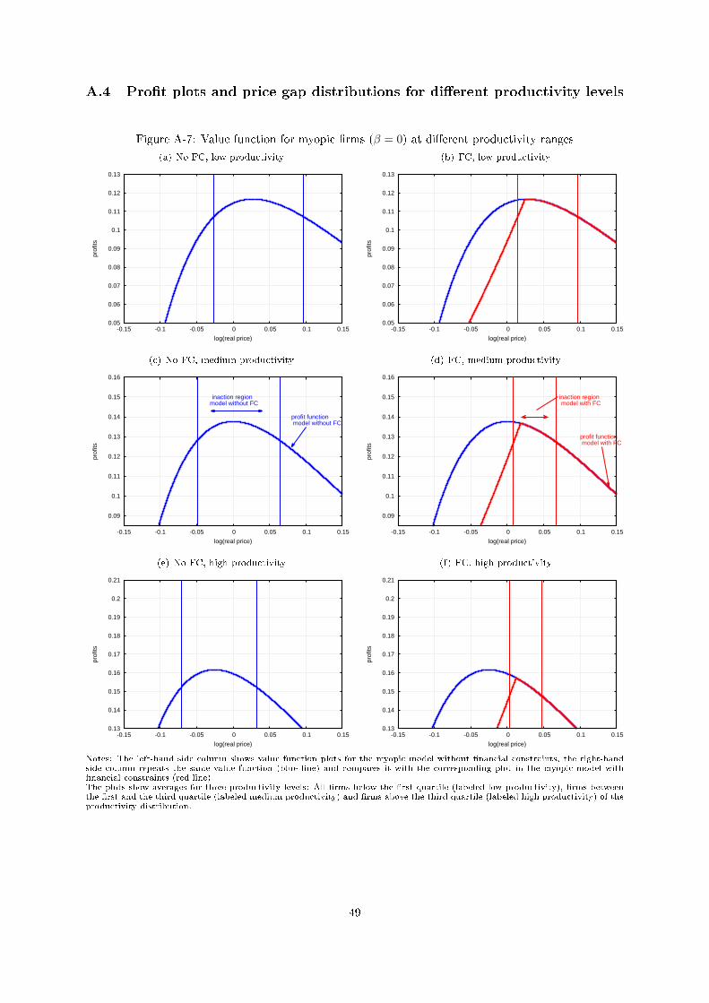
A.4 Pro�t plots and price gap distributions for di�erent productivity levels

Figure A-7: Value function for myopic �rms (β = 0) at di�erent productivity ranges

(a) No FC, low productivity

0.05

0.06

0.07

0.08

0.09

0.1

0.11

0.12

0.13

-0.15 -0.1 -0.05 0 0.05 0.1 0.15

prof

its

log(real price)

(b) FC, low productivity

0.05

0.06

0.07

0.08

0.09

0.1

0.11

0.12

0.13

-0.15 -0.1 -0.05 0 0.05 0.1 0.15

prof

its

log(real price)

(c) No FC, medium productivity

0.09

0.1

0.11

0.12

0.13

0.14

0.15

0.16

-0.15 -0.1 -0.05 0 0.05 0.1 0.15

prof

its

log(real price)

profit function model without FC

inaction region model without FC

(d) FC, medium productivity

0.09

0.1

0.11

0.12

0.13

0.14

0.15

0.16

-0.15 -0.1 -0.05 0 0.05 0.1 0.15

prof

its

log(real price)

profit function model with FC

inaction region model with FC

(e) No FC, high productivity

0.13

0.14

0.15

0.16

0.17

0.18

0.19

0.2

0.21

-0.15 -0.1 -0.05 0 0.05 0.1 0.15

prof

its

log(real price)

(f) FC, high productivity

0.13

0.14

0.15

0.16

0.17

0.18

0.19

0.2

0.21

-0.15 -0.1 -0.05 0 0.05 0.1 0.15

prof

its

log(real price)

Notes: The left-hand side column shows value function plots for the myopic model without �nancial constraints, the right-handside column repeats the same value function (blue line) and compares it with the corresponding plot in the myopic model with�nancial constraints (red line).The plots show averages for three productivity levels: All �rms below the �rst quartile (labeled low productivity), �rms betweenthe �rst and the third quartile (labeled medium productivity) and �rms above the third quartile (labeled high productivity) of theproductivity distribution.

49

Figure A-8: Real price distributions (before adjustment) in the myopic model with and without �nancialconstraint by productivity level

(a) Model without �nancial constraint, low productivity (b) Model with �nancial constraint, low productivity

(c) Model without �nancial constraint, medium productivity (d) Model with �nancial constraint, medium productivity

(e) Model without �nancial constraint, high productivity (f) Model with �nancial constraint, high productivity

Notes: The histograms display the distribution of real prices log(pi), where pi is �rm i's price before price adjustment. Thesolid vertical lines mark the respective inaction region for �rms exactly at the cuto�. Unlike in Figure 3 in the main text, thedistributions are not normalized by the optimal reset price.The left-hand side column shows plots for the myopic model without �nancial constraints, the right-hand side column documentsthe corresponding plot in the myopic model with �nancial constraints.All �rms below the �rst quartile (labeled low productivity), �rms between the �rst and the third quartile (labeled mediumproductivity) and �rms above the third quartile (labeled high productivity) of the productivity distribution.

50

Figure A-9: Real price distributions (before adjustment) in the dynamic model with and without �nancialconstraint by productivity level

(a) Model without �nancial constraint, low productivity (b) Model with �nancial constraint, low productivity

(c) Model without �nancial constraint, medium productivity (d) Model with �nancial constraint, medium productivity

(e) Model without �nancial constraint, high productivity (f) Model with �nancial constraint, high productivity

Notes: The histograms display the distribution of real prices log(pi), where pi is �rm i's price before price adjustment. Thesolid vertical lines mark the respective inaction region for �rms exactly at the cuto�. Unlike in Figure 3 in the main text, thedistributions are not normalized by the optimal reset price.The left-hand side column shows plots for the myopic model without �nancial constraints, the right-hand side column documentsthe corresponding plot in the myopic model with �nancial constraints.All �rms below the �rst quartile (labeled low productivity), �rms between the �rst and the third quartile (labeled mediumproductivity) and �rms above the third quartile (labeled high productivity) of the productivity distribution.

51

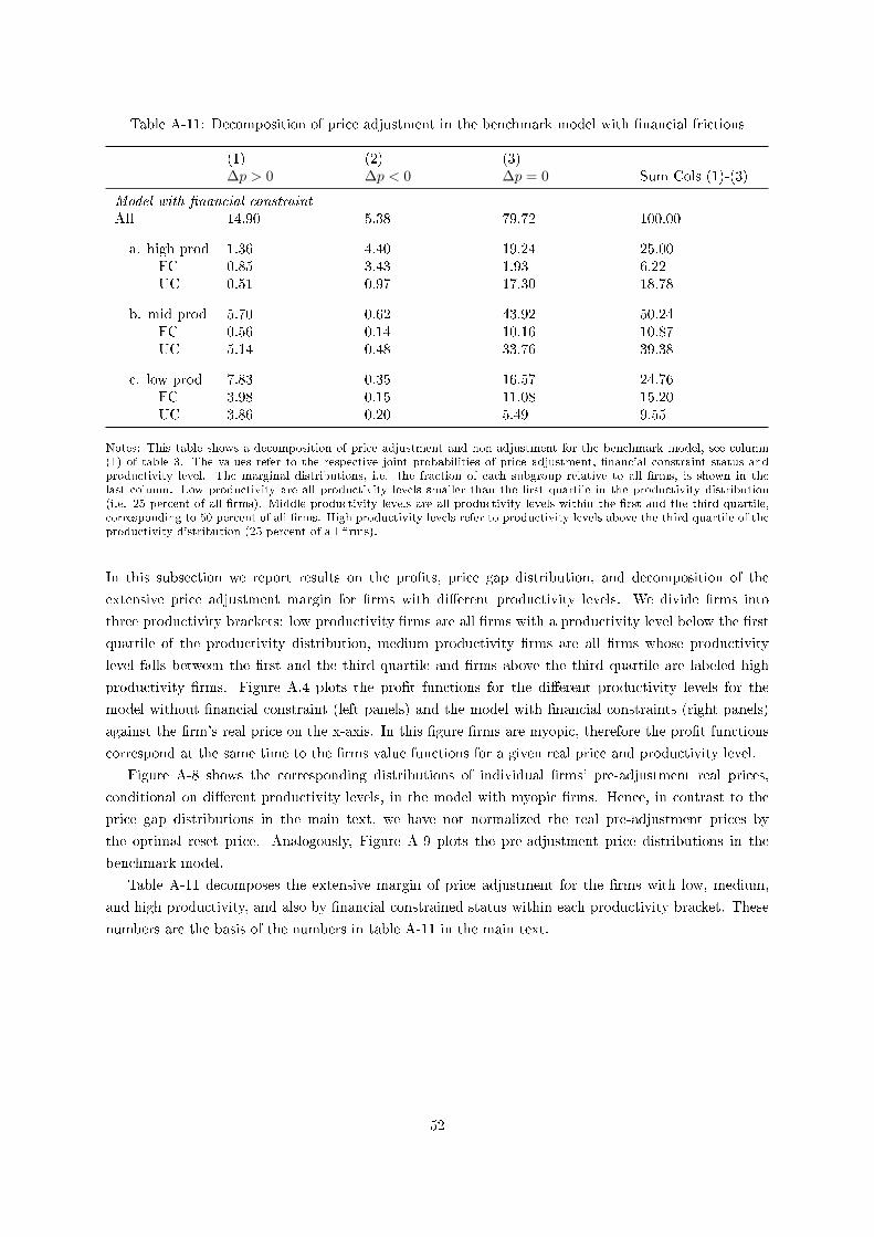
Table A-11: Decomposition of price adjustment in the benchmark model with �nancial frictions

(1) (2) (3)∆p > 0 ∆p < 0 ∆p = 0 Sum Cols (1)-(3)

Model with �nancial constraintAll 14.90 5.38 79.72 100.00

a. high prod 1.36 4.40 19.24 25.00FC 0.85 3.43 1.93 6.22UC 0.51 0.97 17.30 18.78

b. mid prod 5.70 0.62 43.92 50.24FC 0.56 0.14 10.16 10.87UC 5.14 0.48 33.76 39.38

c. low prod 7.83 0.35 16.57 24.76FC 3.98 0.15 11.08 15.20UC 3.86 0.20 5.49 9.55

Notes: This table shows a decomposition of price adjustment and non-adjustment for the benchmark model, see column(1) of table 3. The values refer to the respective joint probabilities of price adjustment, �nancial constraint status andproductivity level. The marginal distributions, i.e. the fraction of each subgroup relative to all �rms, is shown in thelast column. Low productivity are all productivity levels smaller than the �rst quartile in the productivity distribution(i.e. 25 percent of all �rms). Middle productivity levels are all productivity levels within the �rst and the third quartile,corresponding to 50 percent of all �rms. High productivity levels refer to productivity levels above the third quartile of theproductivity distribution (25 percent of all �rms).

In this subsection we report results on the pro�ts, price gap distribution, and decomposition of the

extensive price adjustment margin for �rms with di�erent productivity levels. We divide �rms into

three productivity brackets: low productivity �rms are all �rms with a productivity level below the �rst

quartile of the productivity distribution, medium productivity �rms are all �rms whose productivity

level falls between the �rst and the third quartile and �rms above the third quartile are labeled high

productivity �rms. Figure A.4 plots the pro�t functions for the di�erent productivity levels for the

model without �nancial constraint (left panels) and the model with �nancial constraints (right panels)

against the �rm's real price on the x-axis. In this �gure �rms are myopic, therefore the pro�t functions

correspond at the same time to the �rms value functions for a given real price and productivity level.

Figure A-8 shows the corresponding distributions of individual �rms' pre-adjustment real prices,

conditional on di�erent productivity levels, in the model with myopic �rms. Hence, in contrast to the

price gap distributions in the main text, we have not normalized the real pre-adjustment prices by

the optimal reset price. Analogously, Figure A-9 plots the pre-adjustment price distributions in the

benchmark model.

Table A-11 decomposes the extensive margin of price adjustment for the �rms with low, medium,

and high productivity, and also by �nancial constrained status within each productivity bracket. These

numbers are the basis of the numbers in table A-11 in the main text.

52

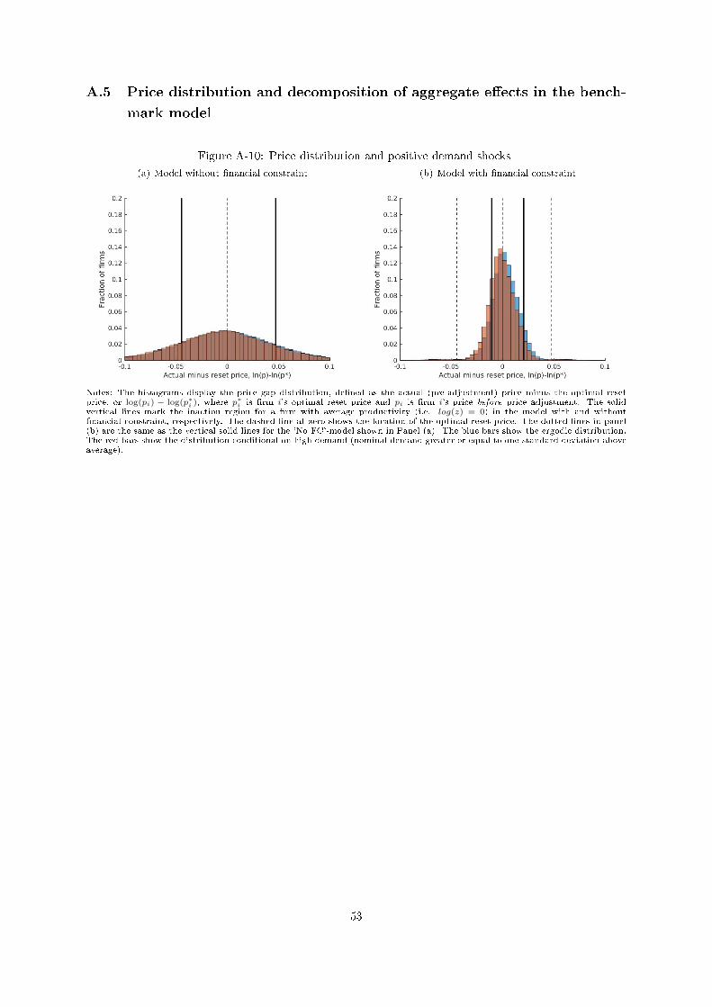
A.5 Price distribution and decomposition of aggregate e�ects in the bench-

mark model

Figure A-10: Price distribution and positive demand shocks

(a) Model without �nancial constraint (b) Model with �nancial constraint

Notes: The histograms display the price gap distribution, de�ned as the actual (pre-adjustment) price minus the optimal resetprice, or log(pi) − log(p∗i ), where p∗i is �rm i's optimal reset price and pi is �rm i's price before price adjustment. The solidvertical lines mark the inaction region for a �rm with average productivity (i.e. log(z) = 0) in the model with and without�nancial constraint, respectively. The dashed line at zero shows the location of the optimal reset price. The dotted lines in panel(b) are the same as the vertical solid lines for the 'No FC'-model shown in Panel (a). The blue bars show the ergodic distribution.The red bars show the distribution conditional on high demand (nominal demand greater or equal to one-standard deviation aboveaverage).

53

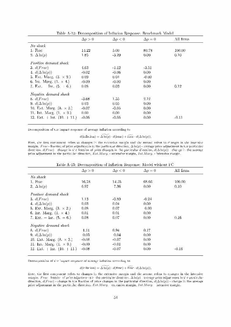
Table A-12: Decomposition of In�ation Response: Benchmark Model

∆p > 0 ∆p < 0 ∆p = 0 All �rms

No shock1. Frac 14.22 5.00 80.78 100.002. ∆ ln(p) 1.85 -3.29 0.00 0.10

Positive demand shock3. d(Frac) 4.63 -1.12 -3.514. d(∆ ln(p)) -0.02 -0.06 0.005. Ext. Marg. (3. × 2.) 0.09 0.04 -0.006. Int. Marg. (1. × 4.) -0.00 -0.00 0.007. Ext. + Int. (5. + 6.) 0.08 0.03 0.00 0.12

Negative demand shock8. d(Frac) -3.68 1.55 2.129. d(∆ ln(p)) 0.03 0.05 0.0010. Ext. Marg. (8. × 2.) -0.07 -0.05 0.0011. Int. Marg. (1. × 9.) 0.00 0.00 0.0012. Ext. + Int. (10. + 11.) -0.06 -0.05 0.00 -0.11

Decomposition of the impact response of average in�ation according to

d(in�ation) = ∆ ln(p) · d(Frac) + Frac · d(∆ ln(p)),

Here, the �rst component refers to changes in the extensive margin and the second refers to changes in the intensivemargin. Frac - fraction of price adjustments in the particular direction, ∆ ln(p) - average price adjustment in the particulardirection, d(Frac) - change in the fraction of price changes in the particular direction, d(∆ ln(p)) - change in the averageprice adjustment in the particular direction, Ext.Marg. - extensive margin, Int.Marg. - intensive margin.

Table A-13: Decomposition of In�ation Response: Model without FC

∆p > 0 ∆p < 0 ∆p = 0 All �rms

No shock1. Frac 16.78 14.55 68.66 100.002. ∆ ln(p) 6.97 -7.36 0.00 0.10

Positive demand shock3. d(Frac) 1.13 -0.89 -0.244. d(∆ ln(p)) 0.03 0.04 0.005. Ext. Marg. (3. × 2.) 0.08 0.07 -0.006. Int. Marg. (1. × 4.) 0.01 0.01 0.007. Ext. + Int. (5. + 6.) 0.08 0.07 0.00 0.16

Negative demand shock8. d(Frac) -1.11 0.94 0.179. d(∆ ln(p)) -0.03 -0.04 0.0010. Ext. Marg. (8. × 2.) -0.08 -0.07 0.0011. Int. Marg. (1. × 9.) -0.00 -0.01 0.0012. Ext. + Int. (10. + 11.) -0.08 -0.07 0.00 -0.16

Decomposition of the impact response of average in�ation according to

d(in�ation) = ∆ ln(p) · d(Frac) + Frac · d(∆ ln(p)),

Here, the �rst component refers to changes in the extensive margin and the second refers to changes in the intensivemargin. Frac - fraction of price adjustments in the particular direction, ∆ ln(p) - average price adjustment in the particulardirection, d(Frac) - change in the fraction of price changes in the particular direction, d(∆ ln(p)) - change in the averageprice adjustment in the particular direction, Ext.Marg. - extensive margin, Int.Marg. - intensive margin.

54

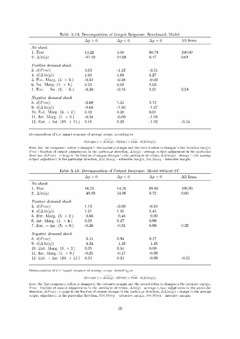
Table A-14: Decomposition of Output Response: Benchmark Model

∆p > 0 ∆p < 0 ∆p = 0 All �rms

No shock1. Frac 14.22 5.00 80.78 100.002. ∆ ln(y) -11.29 24.69 0.47 0.01

Positive demand shock3. d(Frac) 4.63 -1.12 -3.514. d(∆ ln(y)) 1.60 1.89 1.275. Ext. Marg. (3. × 2.) -0.52 -0.28 -0.026. Int. Marg. (1. × 4.) 0.23 0.09 1.037. Ext. + Int. (5. + 6.) -0.30 -0.18 1.01 0.54

Negative demand shock8. d(Frac) -3.68 1.55 2.129. d(∆ ln(y)) -1.69 -1.80 -1.2710. Ext. Marg. (8. × 2.) 0.42 0.38 0.0111. Int. Marg. (1. × 9.) -0.24 -0.09 -1.0312. Ext. + Int. (10. + 11.) 0.18 0.29 -1.02 -0.54

Decomposition of the impact response of average output according to

d(output) = ∆ ln(y) · d(Frac) + Frac · d(∆ ln(y)),

Here, the �rst component refers to changes in the extensive margin and the second refers to changes in the intensive margin.Frac - fraction of output adjustments in the particular direction, ∆ ln(y) - average output adjustment in the particulardirection, d(Frac) - change in the fraction of output changes in the particular direction, d(∆ ln(y)) - change in the averageoutput adjustment in the particular direction, Ext.Marg. - extensive margin, Int.Marg. - intensive margin.

Table A-15: Decomposition of Output Response: Model without FC

∆p > 0 ∆p < 0 ∆p = 0 All �rms

No shock1. Frac 16.78 14.55 68.66 100.002. ∆ ln(y) -49.83 54.06 0.72 0.00

Positive demand shock3. d(Frac) 1.13 -0.89 -0.244. d(∆ ln(y)) 1.21 1.16 1.455. Ext. Marg. (3. × 2.) -0.56 -0.48 -0.006. Int. Marg. (1. × 4.) 0.20 0.17 0.997. Ext. + Int. (5. + 6.) -0.36 -0.31 0.99 0.32

Negative demand shock8. d(Frac) -1.11 0.94 0.179. d(∆ ln(y)) -1.24 -1.16 -1.4510. Ext. Marg. (8. × 2.) 0.55 0.51 0.0011. Int. Marg. (1. × 9.) -0.21 -0.17 -0.9912. Ext. + Int. (10. + 11.) 0.34 0.34 -0.99 -0.31

Decomposition of the impact response of average output according to

d(output) = ∆ ln(y) · d(Frac) + Frac · d(∆ ln(y)),

Here, the �rst component refers to changes in the extensive margin and the second refers to changes in the intensive margin.Frac - fraction of output adjustments in the particular direction, ∆ ln(y) - average output adjustment in the particulardirection, d(Frac) - change in the fraction of output changes in the particular direction, d(∆ ln(y)) - change in the averageoutput adjustment in the particular direction, Ext.Marg. - extensive margin, Int.Marg. - intensive margin.

55

A.6 Partial equilibrium models with alternative mechanisms to generate

price stickiness

The subsection discusses the implications for price adjustment of working capital constraints in a model

with nominal rigidities in the tradition of Calvo (1983) and a model with convex price adjustment costs

as in Rotemberg (1982). The �rst purpose of this subsection is to show analytically why in these type

of models aggregate output responds less when �nancial frictions are present compared to the situation

when the �nancial constraint is removed. For this purpose we use log-linearization techniques. Second,

we brie�y describe how we numerically implement and parameterize the models.

A.6.1 Exogenous Probability of Price Adjustment (Calvo (1983))

In this subs section, we replace the �xed menu cost of price adjustment by nominal rigidities in the

tradition of Calvo (1983) which means that every �rm faces an exogenously given probability f ∈ (0, 1)

per period for not being allowed to adjust its price. With probability (1 − f) the �rm is allowed to

optimally reset its price. Adjustments are assumed to be costless irrespective of their magnitude. f

corresponds to the so called Calvo parameter. Non-adjusters simply continue to sell their products at

previous period's price: pnait = pit−1. When choosing the optimal price pait, adjusters take into account

that with certain probability, the nominal price chosen today will be retained in the future, e.g. pit+1 = paitwith probability f . The law of large numbers implies that in each period the fraction of non-adjusters

is equal to f and their average price is equal to previous period's economy-wide average nominal price,

i.e. Pnat = Pt−1.

The Lagrangean for the problem of a �rm allowed to adjust its price in period t reads

L = Et

∞∑j=0

βjf j{pitPt+j

zit+jhit+j − whit+j}

+ Et

∞∑j=0

βjf j{γit+j

(ξ + ξ

pitPt+j

zit+jhit+j − whit+j)}

(A.8)

+ Et

∞∑j=0

βjf j

{δit+j

((pitPt+j

)−θCt+j − zit+jhit+j

)},

where δit denotes the Lagrangean multiplier associated with the demand constraint, Et is the expectation

operator conditional on period t information, hit is labor input of �mr i, zit denotes the productivity

shock of �rm i, and Pt,Ct denote the aggregate nominal price level and aggregate demand, respectively.

The �rst order conditions with respect to hit and pit read:

δit = (1 + γitξ)pitPt− (1 + γit)

w

zit, (A.9)

Et

∞∑j=0

βjf j

{(1 + γit+jξ)

zit+jhit+jPt+j

− θδit+j(pitPt+j

)−θ−1Ct+jPt+j

}= 0, (A.10)

56

γit

{ξ

(1 +

pitPtzithit

)− whit

}= 0

(A.11)

γit ≥ 0, ξ

(1 +

pitPtzithit

)≥ whit.

δit

{(pitPt

)−θCt − zithit

}= 0

(A.12)

δit ≥ 0,

(pitPt

)−θCt ≥ zithit.

Since we focus on the reaction to an unexpected change in the aggregate price level Pt, we assume

that idiosyncratic productivity does not deviate from the path expected prior to the occurrence of the

aggregate shock. For simplicity, we assume {zit+j}∞j=0 = z. Replacing this �at pro�le by a given

but non-constant path, will make the derivations considerably more tedious without delivering di�erent

implications or further insights. Next, recall that by assumption, nominal aggregate demand St =

PtCt follows a Random Walk with drift µ, logSt = µ + logSt−1 + ηt. Since throughout the paper

we assume Ct = C ∀t, the disturbances ηt correspond to one-time shifts in the aggregate in�ation rate

logPt− logPt−1 and, at the same time, to permanent shifts in the nominal price level Pt. The permanent

nature of the changes in Pt combined with the purely static structure of the two constraints on the one

hand and the assumption on the path of zit, implies that if a constraint is binding (non-binding) today

it will be expected to be binding (non-binding) over the entire future. Furthermore, it is straightforward

to show that, as in the menu-cost model as well as the Rotemberg model, a price adjuster will always

decide to be located on her demand schedule, i.e. will avoid rationing.

Accordingly, we have(pitPt

)−θCt = zithit while equation (A.9) simply determines the value of the

Lagrangean multiplier δit for given paths of the other endogenous variables. Moreover, we can reduce

the system (A.9) through (A.12) to

(θ − 1)Et

∞∑j=0

βjf j

{(1 + γit+jξ)

(pitPt+j

)−θCt+jPt+j

}=

(A.13)

= θEt

∞∑j=0

βjf j

{(1 + γit+j)

w

zit+j

(pitPt+j

)−θ−1Ct+jPt+j

},

and

γit

{ξ

(1 +

(pitPt

)1−θ

Ct

)− w

zit

(pitPt

)−θCt

}= 0

(A.14)

γit ≥ 0, ξ

(1 +

(pitPt

)1−θ

Ct

)≥ w

zit

(pitPt

)−θCt.

57

To derive the dynamics resulting from (A.13) and (A.14), we log-linearize these conditions and view

the system as a piecewise linear one in the sense of Guerrieri and Iacoviello (2015). Without loss of

generality, we log-linearize around pi = P and zi = 1. There are two relevant cases: a slack and a

binding �nancial constraint. In the former, the Lagrange multiplier {γit+j}∞j=0 = 0 and (A.13) reduces

to its well known form lying at the heart of the New Keynesian Phillips Curve:

(θ − 1)Et

∞∑j=0

βjf j

{(pitPt+j

)−θCt+jPt+j

}= θEt

∞∑j=0

βjf j

{w

zit+j

(pitPt+j

)−θ−1Ct+jPt+j

}.

Log-linearizing and rearranging yields

1

1− βfpit =

∞∑j=0

βjf jEtPt+j −∞∑j=0

βjf jEtzit+j .

Thus, if zit = 0 ∀t and the shock to the aggregate price level is permanent, i.e. Pt = Pt+j ∀j ≥ 1, we

obtain

pit = Pt − (1− βf)

∞∑j=0

βjf jEtzit+j .

In other words, unconstrained adjusters approximately completely pass-through permanent shifts in Pt

to their individual nominal prices pit. The same holds for price adjusters facing a binding borrowing con-

straint. For in that case the choice of the optimal price is restricted by (A.14) with ξ

(1 +

(pitPt

)1−θCt

)=

wzit

(pitPt

)−θCt while (A.13) simply determines the path of the Lagrangean multiplier γit for a given path

of the individual nominal price. Log-linearization and rearranging yields

pit = Pt −w

ξ(1− θ) + θwzit.

In sum, price adjusters choose a complete pass-through of changes in the aggregate price level Pt to

their individual prices pit, irrespective of whether they face a slack or a binding �nancial constraint. In

fact, independent of the presence of a �nancial constraint, the average price Pt responds to permanent

changes in Pt as follows:ˆPt = (1− f)Pt,

ˆPt+1 = f(1− f)Pt,ˆPt+2 = f2(1− f)Pt and so on. This is the

case since in each period, a new fraction (1− f) of the �rms who had not yet been able to react to the

shock in Pt are given this opportunity. They respond by applying complete pass-through.

The only di�erence between the economy with and the one without the �nancial friction results from

non-adjusters. In a world without credit market frictions, each �rm operates at its demand curve. If,

however, �rm's behavior is restricted by a borrowing limit, some non-adjusters - those facing a binding

�nancial constraint - will have to produce o� their demand schedule and thus ration demand. Since the

fraction of such �rms increases in the case of a positive innovation to the aggregate price level Pt, output

losses due to rationing increase, causing the output to increase by less than in a world without �nancial

frictions.

A.6.2 Convex Price-Adjustment Costs (Rotemberg (1982))

In this section, we replace the �xed menu cost of price adjustment by a convex price-adjustment cost

function like in Rotemberg (1982). Everything else remains unchanged. For simplicity and as usually

done in the literature, we assume that the price-adjustment cost function is quadratic and equal across

58

�rms. In particular, each change of the individual nominal price is associated with costs amounting to

κ2

(pitpit−1

−Π)2

Ct where κ > 0 and Ct is aggregate demand. The parameter κ measures the degree of

price rigidity and, as we will show below, a�ects the slope of the individual supply curve. Π = 1 + µ is

the gross rate of growth in nominal aggregate demand.37

Each �rm chooses its nominal price pit such that the present discounted value of current and future

pro�ts is maximized subject to the demand and the borrowing constraint. It is easy to show that the

demand constraint is always binding. Thus, we can replace yit by the demand function(pitPt

)−θCt. The

resulting Langrangean reads

L =

(pitPt

)−θCt

(pitPt− w

zit

)− κ

2

(pitpit−1

−Π

)2

Ct

+ γit

(ξ

(1 +

(pitPt

)1−θ

Ct

)− w

zit

(pitPt

)−θCt

)(A.15)

+ Et

{β

(...− κ

2

(pit+1

pit−Π

)2

Ct+1 + ...

)}+ ...,

where γit is the Lagrange multiplier associated with the �nancial constraint and, to save on space, we

neglect terms independent of pit. The �rst order condition with respect to pit reads

(1− θ)(pitPt

)−θ+ θ(1 + γit)

w

zit

(pitPt

)−θ−1

+ γitξ(1− θ)(PitPt

)−θ=

(A.16)

θ(Πit −Π)Πit

(pitPt

)−1

− βθEt

{(Πit+1 −Π)Πit+1

(pitPt

)−1Ct+1

Ct

},

and

γit

{ξ

(1 +

(pitPt

)1−θ

Ct

)− w

zit

(pitPt

)−θCt

}= 0

(A.17)

γit ≥ 0, ξ

(1 +

(pitPt

)1−θ

Ct

)≥ w

zit

(pitPt

)−θCt.

where Πit = pit/pit−1 is the �rm-speci�c gross rate of in�ation. Equations (A.16) and (A.17) represent

the �rm speci�c supply curve. If the �nancial constraint does not bind, the optimal pricing decision

is determined by (A.16) with γit = 0. In contrast, if the �nancial constraint binds, pit is derived from

(A.17) with ξ

(1 +

(pitPt

)1−θCt

)= w

zit

(pitPt

)−θCt while (A.16) determines the value of the Lagrange

multiplier γit.

The easiest way to derive the main tendencies implied by (A.16) and (A.17) is by log-linearizing

them and viewing the system as a piecewise linear one in the sense of Guerrieri and Iacoviello (2015).

Without loss of generality, we log-linearize around pi = P and zi = 1. In addition, since we focus on the

e�ects of unexpected changes in Pt, we assume that zit does not deviate from its initial value zi. If the

�nancial constraint is not binding, the optimal pricing decision is approximately determined according

37If Ct = C ∀t, then µ corresponds to the aggregate in�ation rate.

59

to the log-linear version of (A.16) with γit = 0:

pit =θ − 1

θ − 1 + κ(1 + β)(Pt − zit)

+κ

θ − 1 + φ(1 + β)pit−1 +

βκ

θ − 1 + κ(1 + β)Etpit+1, (A.18)

where xt = (xt− x)/x denotes a relative deviation from the point around which we linearize. It is easily

seen from (A.18) that in the short run, temporary as well as permanent shocks to the aggregate price level

Pt are incompletely passed through to changes in the individual nominal price pit since the coe�cient in

front of Pt,θ−1

θ−1+κ(1+β) , lies within the open interval (0, 1).38 In contrast, when the �nancial constraint

binds, the �rm sets its price according to the constraint itself,

ξ

(1 +

(pitPt

)1−θ

Ct

)=

w

zit

(pitPt

)−θCt.

Log-linearizing the last equation yields

pit = Pt −w

ξ(1− θ) + θwzit. (A.19)

Obviously, (A.19) implies that if the �rm is restricted by its borrowing limit, its optimal pricing decision

will be approximately associated with full pass-through of movements in the aggregate price level Pt to

changes in the individual price pit. The intuition is as follows: The borrowing limit actually works as a

capacity constraint imposing an upper bound on the quantity the �rm is able to produce. As soon as full

capacity is reached, the individual supply curve becomes approximately (up to a linear approximation)

vertical. Any further increases of demand can only be accommodated by raising �rm's prices but not by

expanding production. In other words, any shifts of the demand curve - due to changes in the economy-

wide variables Pt or in Ct - represent shifts along an approximately vertical individual supply schedule

and thus, are associated with no quantity but a relatively strong price reaction.

Based on the discussion in this section, it is easy to understand why an economy free of �nancial

frictions will respond to exogenous permanent shifts in the aggregate price level Pt di�erently from

an economy subject to our borrowing constraint. In the former, each �rm sets its optimal nominal

price according to (A.18). Hence, the shock to Pt is not fully transmitted to the average price level

Pt =∑Ni=1 pit, where N is the number of �rms, with the degree of pass-through being approximately

equal across �rms. In contrast, if the economy is subject to our �nancial friction and there is a strictly

positive fraction of �rms facing a binding constraint, only part of the �rms - the unconstrained ones

- will set prices according to (A.18). The rest - for which the constraint binds - will choose to fully

pass the shift in Pt through to their individual prices pit. Accordingly, the pass-through from Pt to

the average nominal price level Pt will be relatively more complete. Consequently, given the downward

sloping demand curve, the average output response in an economy subject to the �nancial constraint

will tend to be relatively weaker. Note further, that in the case of positive shocks to Pt, the di�erence

between the two economies is further magni�ed as the fraction of �nancially constrained �rms increases.

38Note that the short-run pass-through of movements in Pt to changes in pit is incomplete even if the shift in Pt ispermanent as is the case with our assumed process for Pt, i.e. log(St) = µ + log(St−1) + ηt where nominal demand

St = PtCt and Ct = const. To see this, consider two polar cases: Etpit+1 = Pt and Etpit+1 = pit. In the former, the

coe�cient linking pit and Pt in the short run becomes θ−1+βκθ−1+f(1+β)

which is strictly larger than zero and smaller than

unity. In the case Etpit+1 = pit, the corresponding coe�cient becomes θ−1θ−1+f

which also lies within (0, 1).

60

The opposite happens - the di�erence between the economy with and the one without �nancial frictions

becomes smaller - when there is a permanent drop in Pt since the number of �rms with a binding credit

constraint decreases.

A.6.3 Numerical Implementation and Parametrization

For the results reported in the main text we solve both the Calvo and the Rotemberg model by value

function iteration. To be more precise, we solve a version of the Calvo model as in Nakamura and

Steinsson (2010) where �rms with probability 1− α draw a �x cost (fH) and with probability α draw a

low �x cost (fL). We then solve the model by value. In practice we set fL = 0 and fH to a very high

value, so that �rms that draw the high �x cost never adjust prices and �rms that draw the zero �x cost

always adjust. We then calibrate the fraction 1− α to match the average frequency of price adjustment

in our data.

For the Rotemberg model, we set the menu cost to zero but introduce quadratic adjustment costs.

Given the �rm's beginning of period nominal price pit, the end-of-period nominal price qit, the aggregate

price level Pt, and idiosyncratic productivity zit, the value function of �rm i in the Rotemberg model is

given by

V (pit/Pt, zit) = maxqit,hit

(qitPt− w

zit

)zithit − κ

2

(qitpit− eµ

)2

C + βEtV (qit/Pt+1, zit+1)

s.t. zithit ≤ qitPt

−θC

whit ≤ ξ(1 + qitPtzithit)

where we have assumed that Ct = C for all t and that the adjustment costs are de�ned relative to the

average gross in�ation rate eµ. As in the benchmark model, we solve both models presented here using

value function iteration on a discretized productivity and price grid.

We have parameterized the models in the following way. The discount factor and the demand elasticity

are calibrated as in the benchmark model, equal to 7.25 and 0.961/12, respectively. For simplicity, the

parameters of the shock process are calibrated as in the benchmark model. The probability of price

adjustment in the Calvo model is set to (1 − α) = 0.22 to match the empirical moment from our

data. The adjustment cost parameter in the Rotemberg model κ is set such that the Calvo model and

the Rotemberg model imply the same level of aggregate nominal rigidity in the absence of �nancial

constraints.

A.6.4 Impulse responses

Figure A-11 show the impulse responses of average output and in�ation to a positive nominal demand

shock in the Calvo and Rotemberg model, respectively, and compare them to the impulse responses of

the benchmark menu cost model.

61

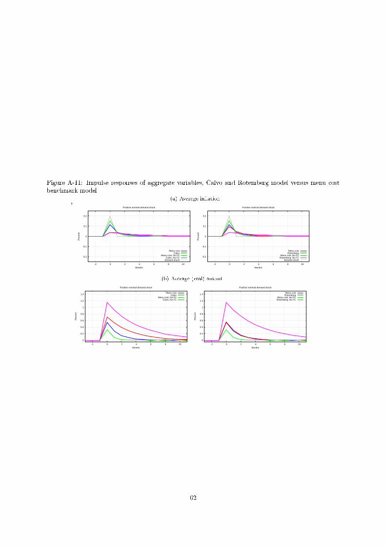
Figure A-11: Impulse responses of aggregate variables, Calvo and Rotemberg model versus menu costbenchmark model

,(a) Average in�ation

-0.2

-0.1

0

0.1

0.2

-2 0 2 4 6 8 10

Per

cent

Months

Positive nominal demand shock

Menu costCalvo

Menu cost, No FCCalvo, No FC

demand shock-0.2

-0.1

0

0.1

0.2

-2 0 2 4 6 8 10

Per

cent

Months

Positive nominal demand shock

Menu costRotemberg

Menu cost, No FCRotemberg, No FC

demand shock

(b) Average (real) output

0

0.2

0.4

0.6

0.8

1

1.2

1.4

-2 0 2 4 6 8 10

Per

cent

Months

Positive nominal demand shock

Menu costCalvo

Menu cost, No FCCalvo, No FC

0

0.2

0.4

0.6

0.8

1

1.2

1.4

-2 0 2 4 6 8 10

Per

cent

Months

Positive nominal demand shock

Menu costRotemberg

Menu cost, No FCRotemberg, No FC

62

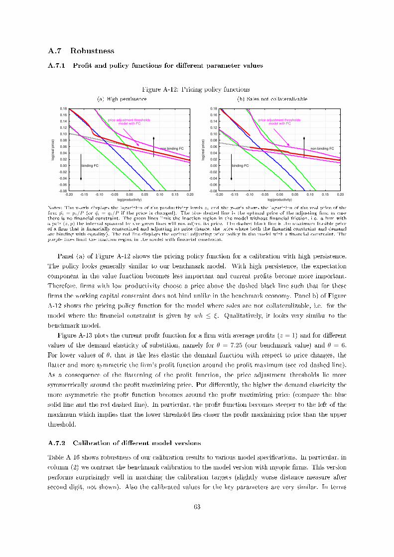
A.7 Robustness

A.7.1 Pro�t and policy functions for di�erent parameter values

Figure A-12: Pricing policy functions

(a) High persistence

-0.08

-0.06

-0.04

-0.02

0.00

0.02

0.04

0.06

0.08

0.10

0.12

0.14

0.16

0.18

-0.20 -0.15 -0.10 -0.05 0.00 0.05 0.10 0.15 0.20

log(r

eal price)

log(productivity)

price adjustment thresholds model with FC

non binding FC

binding FC

(b) Sales not collateralizable

-0.08

-0.06

-0.04

-0.02

0.00

0.02

0.04

0.06

0.08

0.10

0.12

0.14

0.16

0.18

-0.20 -0.15 -0.10 -0.05 0.00 0.05 0.10 0.15 0.20

log(r

eal price)

log(productivity)

price adjustment thresholds model with FC

non binding FC

binding FC

Notes: The x-axis displays the logarithm of the productivity levels zi and the y-axis shows the logarithm of the real price of the�rm pi = pi/P (or qi = qi/P if the price is changed). The blue dashed line is the optimal price of the adjusting �rm in casethere is no �nancial constraint. The green lines limit the inaction region in the model without �nancial friction; i.e. a �rm witha pair (z, p) the interval spanned by the green lines will not adjust its price. The dashed black line is the maximum feasible priceof a �rm that is �nancially constrained and adjusting its price (hence, the price where both the �nancial constraint and demandare binding with equality). The red line displays the optimal adjusting price policy in the model with a �nancial constraint. Thepurple lines limit the inaction region in the model with �nancial constraint.

Panel (a) of Figure A-12 shows the pricing policy function for a calibration with high persistence.

The policy looks generally similar to our benchmark model. With high persistence, the expectation

component in the value function becomes less important and current pro�ts become more important.

Therefore, �rms with low productivity choose a price above the dashed black line such that for these

�rms the working capital constraint does not bind unlike in the benchmark economy. Panel b) of Figure

A-12 shows the pricing policy function for the model where sales are not collateralizable, i.e. for the

model where the �nancial constraint is given by wh ≤ ξ. Qualitatively, it looks very similar to the

benchmark model.

Figure A-13 plots the current pro�t function for a �rm with average pro�ts (z = 1) and for di�erent

values of the demand elasticity of substition, namely for θ = 7.25 (our benchmark value) and θ = 6.

For lower values of θ, that is the less elastic the demand function with respect to price changes, the

�atter and more symmetric the �rm's pro�t function around the pro�t maximum (see red dashed line).

As a consequence of the �attening of the pro�t function, the price adjustment thresholds lie more

symmetrically around the pro�t maximizing price. Put di�erently, the higher the demand elasticity the

more asymmetric the pro�t function becomes around the pro�t maximizing price (compare the blue

solid line and the red dashed line). In particular, the pro�t function becomes steeper to the left of the

maximum which implies that the lower threshold lies closer the pro�t maximizing price than the upper

threshold.

A.7.2 Calibration of di�erent model versions

Table A-16 shows robustness of our calibration results to various model speci�cations. In particular, in

column (2) we contrast the benchmark calibration to the model version with myopic �rms. This version

performs surprisingly well in matching the calibration targets (slightly worse distance measure after

second digit, not shown). Also the calibrated values for the key parameters are very similar. In terms

63

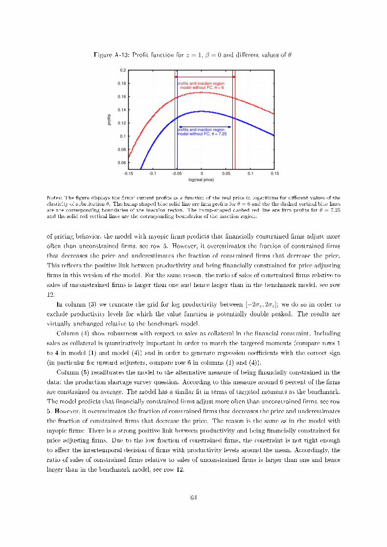
Figure A-13: Pro�t function for z = 1, β = 0 and di�erent values of θ

0.06

0.08

0.1

0.12

0.14

0.16

0.18

0.2

-0.15 -0.1 -0.05 0 0.05 0.1 0.15

pro

fits

log(real price)

profits and inaction region model without FC, θ = 7.25

profits and inaction region model without FC, θ = 6

Notes: The �gure displays the �rms' current pro�ts as a function of the real price in logarithms for di�erent values of theelasticity of substitution θ. The hump-shaped blue solid line are �rm pro�ts for θ = 6 and the the dashed vertical blue linesare the corresponding boundaries of the inaction region. The hump-shaped dashed red line are �rm pro�ts for θ = 7.25and the solid red vertical lines are the corresponding boundaries of the inaction region.

of pricing behavior, the model with myopic �rms predicts that �nancially constrained �rms adjust more

often than unconstrained �rms, see row 5. However, it overestimates the fraction of constrained �rms

that decreases the price and underestimates the fraction of constrained �rms that decrease the price.

This re�ects the positive link between productivity and being �nancially constrained for price adjusting

�rms in this version of the model. For the same reason, the ratio of sales of constrained �rms relative to

sales of unconstrained �rms is larger than one and hence larger than in the benchmark model, see row

12.

In column (3) we truncate the grid for log productivity between [−2σz, 2σz]; we do so in order to

exclude productivity levels for which the value function is potentially double peaked. The results are

virtually unchanged relative to the benchmark model.

Column (4) show robustness with respect to sales as collateral in the �nancial constraint. Including

sales as collateral is quantitatively important in order to match the targeted moments (compare rows 1

to 4 in model (1) and model (4)) and in order to generate regression coe�cients with the correct sign

(in particular for upward adjusters, compare row 6 in columns (1) and (4)).

Column (5) recalibrates the model to the alternative measure of being �nancially constrained in the

data: the production shortage survey question. According to this measure around 6 percent of the �rms

are constrained on average. The model has a similar �t in terms of targeted moments as the benchmark.

The model predicts that �nancially constrained �rms adjust more often than unconstrained �rms, see row

5. However, it overestimates the fraction of constrained �rms that decreases the price and underestimates

the fraction of constrained �rms that decrease the price. The reason is the same as in the model with

myopic �rms: There is a strong positive link between productivity and being �nancially constrained for

price adjusting �rms. Due to the low fraction of constrained �rms, the constraint is not tight enough

to a�ect the intertemporal decision of �rms with productivity levels around the mean. Accordingly, the

ratio of sales of constrained �rms relative to sales of unconstrained �rms is larger than one and hence

larger than in the benchmark model, see row 12.

64

Columns (6) and (7) show the calibration results when we consider values for the elasticity of demand

that are lower and higher, respectively, as compared to the benchmark. The model implications are

similar to the benchmark model. However, the model (6) largely overestimates the fraction of constrained

�rms that increase their price (row 6) and therefore overestimates the price adjustment probability of

�nancially constrained �rms (row 5). The model with higher elasticity of substitution underestimates the

upward price adjustment of �nancially constrained �rms relative to unconstrained �rms (row 6) while

leaving the downward price adjustment of �nancially constrained �rms una�ected (row 7) compared to

the benchmark.

Table A-17 reports robustness results with respect to the idiosyncratic shock persistence. Here, we

increase the shock persistence leaving all other parameters as in the benchmark calibration in order

to show the ceteris paribus e�ect of higher persistence. Two results stand out: First, the only targeted

moments that are sensitive to di�erent values of shock persistence are the fractions of price changes. This

is intuitive as a ceteris paribus change in the persistence changes the variance of the productivity shock.

Hence, higher persistence means larger shocks and a higher probability to be outside the inaction region

if menu costs stay the same. Second, shock persistence a�ects quantitatively our regressions results (see

row 5-7). The main conclusion however is una�ected: for all productivity levels, the model predicts that

�nancially constrained �rms adjust prices more often than unconstrained �rms.

Table A-18 reports the results for a model version where we allow for two types of idiosyncratic shocks:

productivity and �nancial shocks. Financial shocks are modeled as shocks to ξ, i.e. the collateralizable

fraction of capital and sales. In particular log(ξ) follows an AR(1) process with standard deviation σξ

and persistence ρξ.39 In the calibration shown here we assume that �nancial and productivity shocks

have the same persistence ρz = ρξ. We calibrate the variance of the �nancial shock so that median

sales are the same for �nancially constrained and unconstrained �rms, see row 5. Column (1) uses

the benchmark calibration strategy targeting a fraction of 32 percent of �nancially constrained �rms.

This model does not perform better than the benchmark without �nancial shocks. Column (2) uses the

alternative target of 6 percent of constrained �rms as suggested by the production shortage question

in the survey data. In this case, the model performance improves as the model now also predicts that

�nancially constrained �rms adjust more often than unconstrained �rms, see regression coe�cient in row

7. These are likely �rms that are hit by a negative �nancial shock and therefore have to increase their

price as the unconstrained price is no longer attainable given their productivity level.

A.7.3 Aggregate implications of di�erent model versions

Table A-19 shows the on impact impulse responses to a positive aggregate nominal demand shock compar-

ing the di�erent model versions to the benchmark model. All models have the same qualitative message:

the model with �nancial constraints exhibits smaller in�ation responses and larger output responses

than the model without �nancial constraint. In all model versions the fraction of price adjusting �rms

increases signi�cantly in response to the shocks in contrast to the models without �nancial constraints.

39Theoretically log(ξ) follows a truncated normal distribution, so that ξ lies in the interval (0,1). In practice, since wediscretize the state space the bounds are not relevant for the simulation.

65

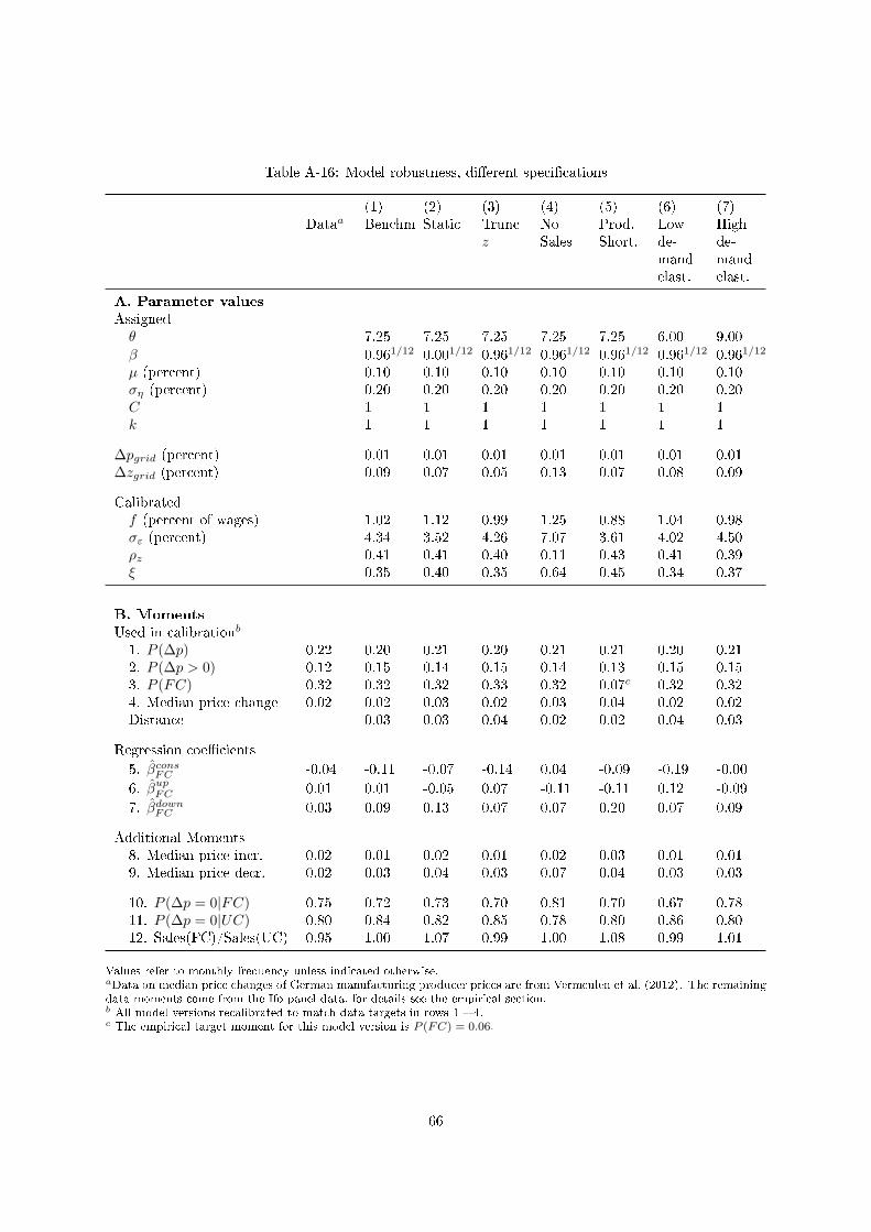
Table A-16: Model robustness, di�erent speci�cations

(1) (2) (3) (4) (5) (6) (7)Dataa Benchm Static Trunc

zNoSales

Prod.Short.

Lowde-mandelast.

Highde-mandelast.

A. Parameter valuesAssignedθ 7.25 7.25 7.25 7.25 7.25 6.00 9.00β 0.961/12 0.001/12 0.961/12 0.961/12 0.961/12 0.961/12 0.961/12

µ (percent) 0.10 0.10 0.10 0.10 0.10 0.10 0.10ση (percent) 0.20 0.20 0.20 0.20 0.20 0.20 0.20C 1 1 1 1 1 1 1k 1 1 1 1 1 1 1

∆pgrid (percent) 0.01 0.01 0.01 0.01 0.01 0.01 0.01∆zgrid (percent) 0.09 0.07 0.05 0.13 0.07 0.08 0.09

Calibratedf (percent of wages) 1.02 1.12 0.99 1.25 0.88 1.04 0.98σε (percent) 4.34 3.52 4.26 7.07 3.61 4.02 4.50ρz 0.41 0.41 0.40 0.11 0.43 0.41 0.39ξ 0.35 0.40 0.35 0.64 0.45 0.34 0.37

B. MomentsUsed in calibrationb

1. P (∆p) 0.22 0.20 0.21 0.20 0.21 0.21 0.20 0.212. P (∆p > 0) 0.12 0.15 0.14 0.15 0.14 0.13 0.15 0.153. P (FC) 0.32 0.32 0.32 0.33 0.32 0.07c 0.32 0.324. Median price change 0.02 0.02 0.03 0.02 0.03 0.04 0.02 0.02Distance 0.03 0.03 0.04 0.02 0.02 0.04 0.03

Regression coe�cients

5. βconsFC -0.04 -0.11 -0.07 -0.14 0.04 -0.09 -0.19 -0.00

6. βupFC 0.01 0.01 -0.05 0.07 -0.11 -0.11 0.12 -0.09

7. βdownFC 0.03 0.09 0.13 0.07 0.07 0.20 0.07 0.09

Additional Moments8. Median price incr. 0.02 0.01 0.02 0.01 0.02 0.03 0.01 0.019. Median price decr. 0.02 0.03 0.04 0.03 0.07 0.04 0.03 0.03

10. P (∆p = 0|FC) 0.75 0.72 0.73 0.70 0.81 0.70 0.67 0.7811. P (∆p = 0|UC) 0.80 0.84 0.82 0.85 0.78 0.80 0.86 0.8012. Sales(FC)/Sales(UC) 0.95 1.00 1.07 0.99 1.00 1.08 0.99 1.01

Values refer to monthly frequency unless indicated otherwise.aData on median price changes of German manufacturing producer prices are from Vermeulen et al. (2012). The remainingdata moments come from the Ifo panel data, for details see the empirical section.b All model versions recalibrated to match data targets in rows 1 � 4.c The empirical target moment for this model version is P (FC) = 0.06.

66

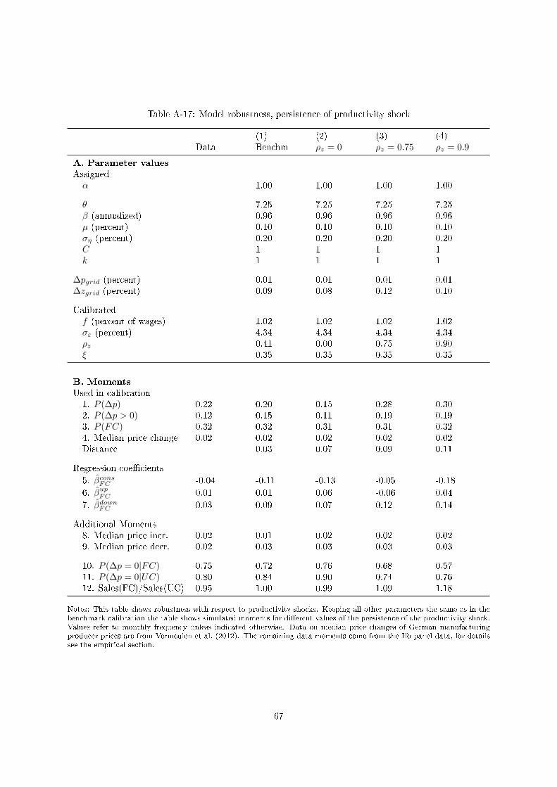
Table A-17: Model robustness, persistence of productivity shock

(1) (2) (3) (4)Data Benchm ρz = 0 ρz = 0.75 ρz = 0.9

A. Parameter valuesAssignedα 1.00 1.00 1.00 1.00

θ 7.25 7.25 7.25 7.25β (annualized) 0.96 0.96 0.96 0.96µ (percent) 0.10 0.10 0.10 0.10ση (percent) 0.20 0.20 0.20 0.20C 1 1 1 1k 1 1 1 1

∆pgrid (percent) 0.01 0.01 0.01 0.01∆zgrid (percent) 0.09 0.08 0.12 0.10

Calibratedf (percent of wages) 1.02 1.02 1.02 1.02σε (percent) 4.34 4.34 4.34 4.34ρz 0.41 0.00 0.75 0.90ξ 0.35 0.35 0.35 0.35

B. MomentsUsed in calibration1. P (∆p) 0.22 0.20 0.15 0.28 0.302. P (∆p > 0) 0.12 0.15 0.11 0.19 0.193. P (FC) 0.32 0.32 0.31 0.31 0.324. Median price change 0.02 0.02 0.02 0.02 0.02Distance 0.03 0.07 0.09 0.11

Regression coe�cients

5. βconsFC -0.04 -0.11 -0.13 -0.05 -0.18

6. βupFC 0.01 0.01 0.06 -0.06 0.04

7. βdownFC 0.03 0.09 0.07 0.12 0.14

Additional Moments8. Median price incr. 0.02 0.01 0.02 0.02 0.029. Median price decr. 0.02 0.03 0.03 0.03 0.03

10. P (∆p = 0|FC) 0.75 0.72 0.76 0.68 0.5711. P (∆p = 0|UC) 0.80 0.84 0.90 0.74 0.7612. Sales(FC)/Sales(UC) 0.95 1.00 0.99 1.09 1.18

Notes: This table shows robustness with respect to productivity shocks. Keeping all other parameters the same as in thebenchmark calibration the table shows simulated moments for di�erent values of the persistence of the productivity shock.Values refer to monthly frequency unless indicated otherwise. Data on median price changes of German manufacturingproducer prices are from Vermeulen et al. (2012). The remaining data moments come from the Ifo panel data, for detailssee the empirical section.

67

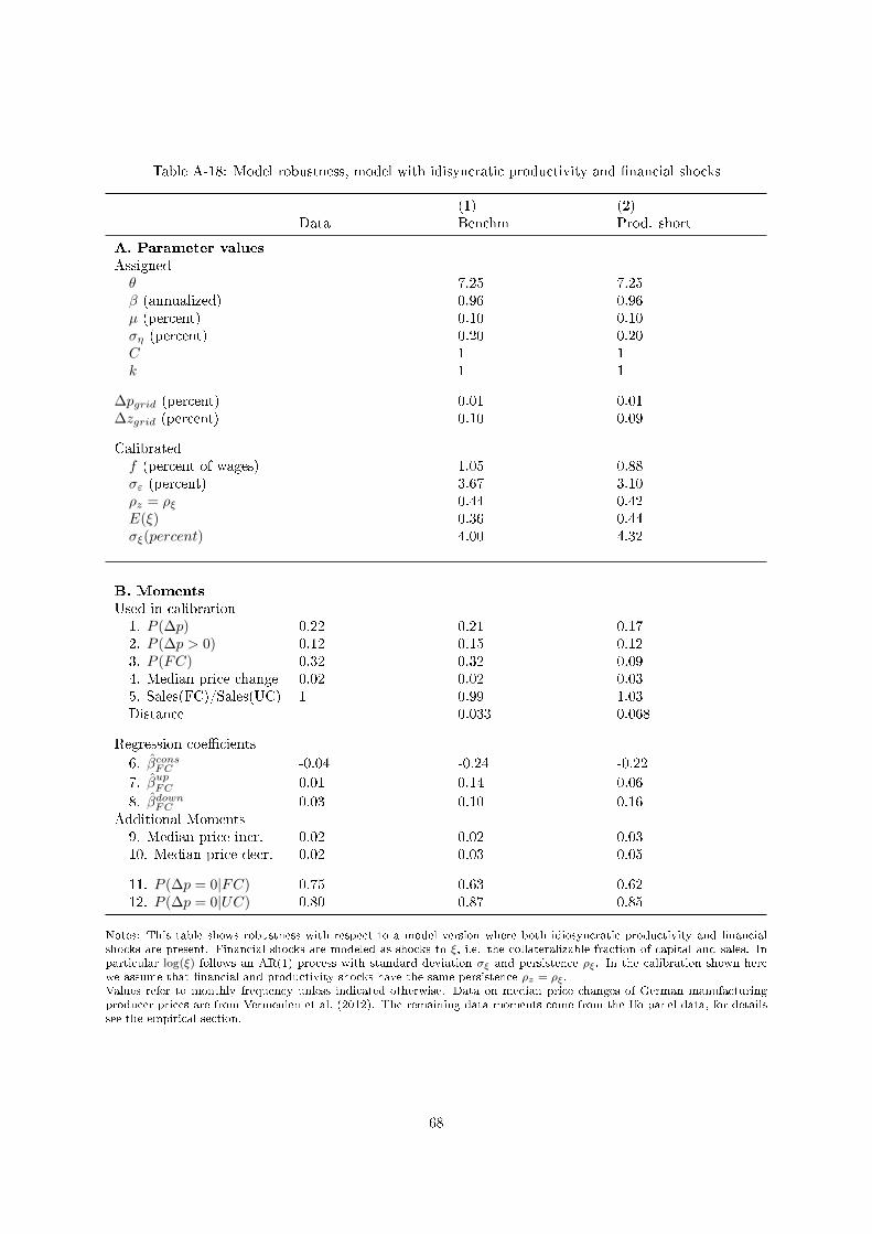
Table A-18: Model robustness, model with idisyncratic productivity and �nancial shocks

(1) (2)Data Benchm Prod. short

A. Parameter valuesAssignedθ 7.25 7.25β (annualized) 0.96 0.96µ (percent) 0.10 0.10ση (percent) 0.20 0.20C 1 1k 1 1

∆pgrid (percent) 0.01 0.01∆zgrid (percent) 0.10 0.09

Calibratedf (percent of wages) 1.05 0.88σε (percent) 3.67 3.10ρz = ρξ 0.44 0.42E(ξ) 0.36 0.44σξ(percent) 4.00 4.32

B. MomentsUsed in calibration1. P (∆p) 0.22 0.21 0.172. P (∆p > 0) 0.12 0.15 0.123. P (FC) 0.32 0.32 0.094. Median price change 0.02 0.02 0.035. Sales(FC)/Sales(UC) 1 0.99 1.03Distance 0.033 0.068

Regression coe�cients

6. βconsFC -0.04 -0.24 -0.22

7. βupFC 0.01 0.14 0.06

8. βdownFC 0.03 0.10 0.16Additional Moments9. Median price incr. 0.02 0.02 0.0310. Median price decr. 0.02 0.03 0.05

11. P (∆p = 0|FC) 0.75 0.63 0.6212. P (∆p = 0|UC) 0.80 0.87 0.85

Notes: This table shows robustness with respect to a model version where both idiosyncratic productivity and �nancialshocks are present. Financial shocks are modeled as shocks to ξ, i.e. the collateralizable fraction of capital and sales. Inparticular log(ξ) follows an AR(1) process with standard deviation σξ and persistence ρξ. In the calibration shown herewe assume that �nancial and productivity shocks have the same persistence ρz = ρξ.Values refer to monthly frequency unless indicated otherwise. Data on median price changes of German manufacturingproducer prices are from Vermeulen et al. (2012). The remaining data moments come from the Ifo panel data, for detailssee the empirical section.

68

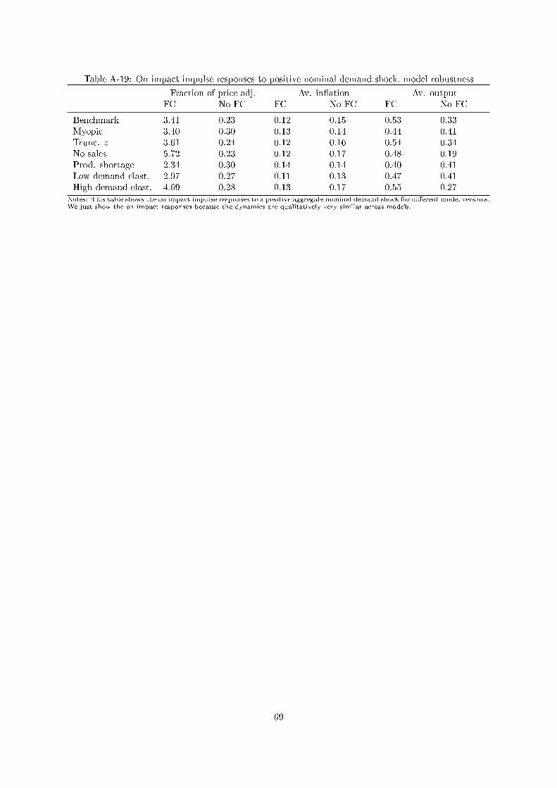
Table A-19: On impact impulse responses to positive nominal demand shock, model robustness

Fraction of price adj. Av. in�ation Av. outputFC No FC FC No FC FC No FC

Benchmark 3.41 0.23 0.12 0.15 0.53 0.33Myopic 3.40 0.30 0.13 0.14 0.44 0.41Trunc. z 3.61 0.24 0.12 0.16 0.54 0.34No sales 5.72 0.23 0.12 0.17 0.48 0.19Prod. shortage 2.34 0.30 0.14 0.14 0.40 0.41Low demand elast. 2.97 0.27 0.11 0.13 0.47 0.41High demand elast. 4.69 0.28 0.13 0.17 0.55 0.27

Notes: This table shows the on impact impulse responses to a positive aggregate nominal demand shock for di�erent model versions.We just show the on impact responses because the dynamics are qualitatively very similar across models.

69