Final Project Part IMATLAB Session
ES 156 Signals and Systems 2007
SEAS
Prepared by Frank Tompkins
Outline
• Discrete Cosine Transform (DCT)– Review of DFT/FFT– 1-D and 2-D
• Basic Image Processing– 2-D LTI systems
• Impulse response• Filtering kernels and fspecial•Thresholding

DFT Review
• Finite length discrete time signal x[n]
• Discrete fourier transform
• fft, ifft, fftshift, ifftshift in MATLAB
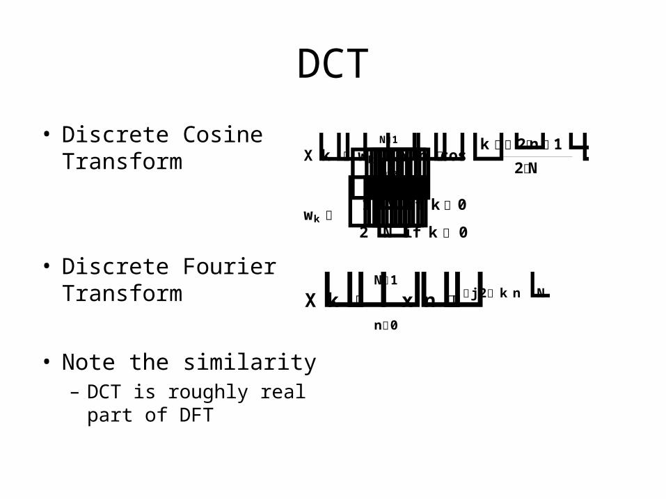
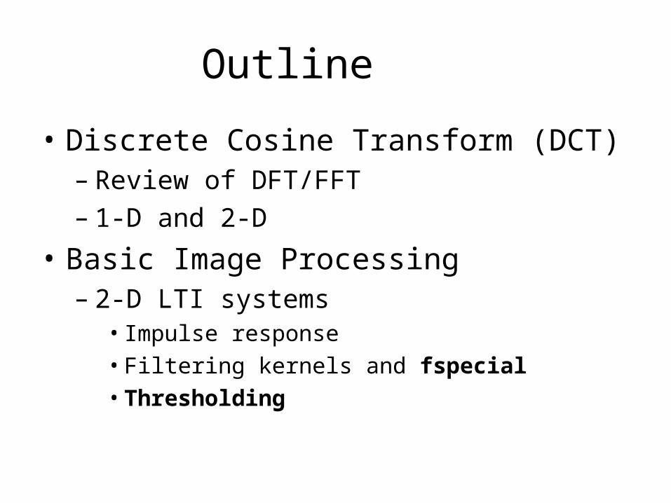
DCT
• Discrete Cosine Transform
• Discrete Fourier Transform
• Note the similarity– DCT is roughly real part
of DFT
Xkn0
N1xnj2 k nN
Xk wkn0
N1xncosk 2n1
2N
wk 1N if k 02N if k 0
2-D Discrete Time Signals
• x[m,n], finite length in both dimensions– Can think of it as a matrix
• Doesn’t have to be square
– An image is one example
• How to do frequency analysis of a 2-D signal?– Just do two Fourier transforms; one for each
dimension

DCT (2-D)
• Each signal/function can be thought of as a matrix• We can treat x[m,n] as a function of m for each n
– Define xn[m] = x[m,n]
• Compute DCT of xn[m], call it Xn[k]• Treat Xn[k] as a function of n for each k
– Define xk[n] = Xn[k]
• Compute DCT of xk[n], call it Xk[l]• Then we define the (2-D) DCT of x[m,n] to be X[k, l] = Xk[l]
DCT
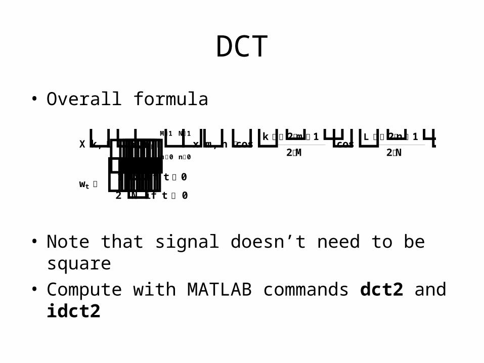
• Overall formula
• Note that signal doesn’t need to be square• Compute with MATLAB commands dct2 and idct2
Xk, L wkwLm0
M1n0
N1xm, ncosk 2m 1
2McosL 2n 1
2N
wt 1N if t 02N if t 0
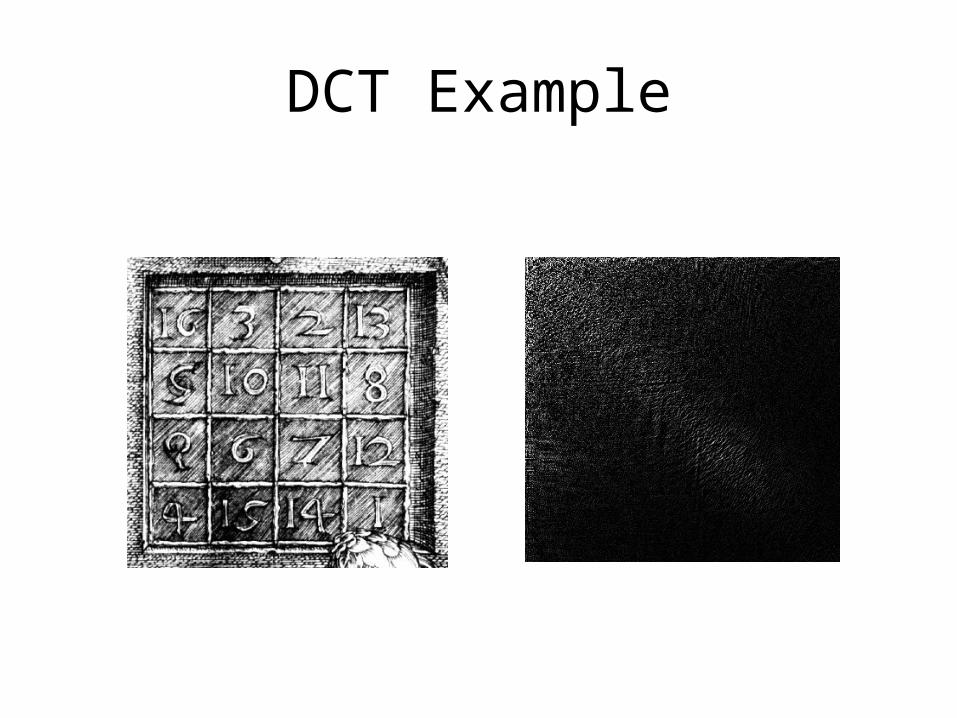
DCT Example
2-D LTI Systems
• In 1-D, LTI systems is characterized entirely by impulse response h[n]
– Input x[n] yields output y[n] = h[n] * x[n]
• For 2-D LTI systems, we have a similar result– Input x[m,n] yields output
y[m,n] = h[m,n] ** x[m,n]
• This is a 2-D convolution
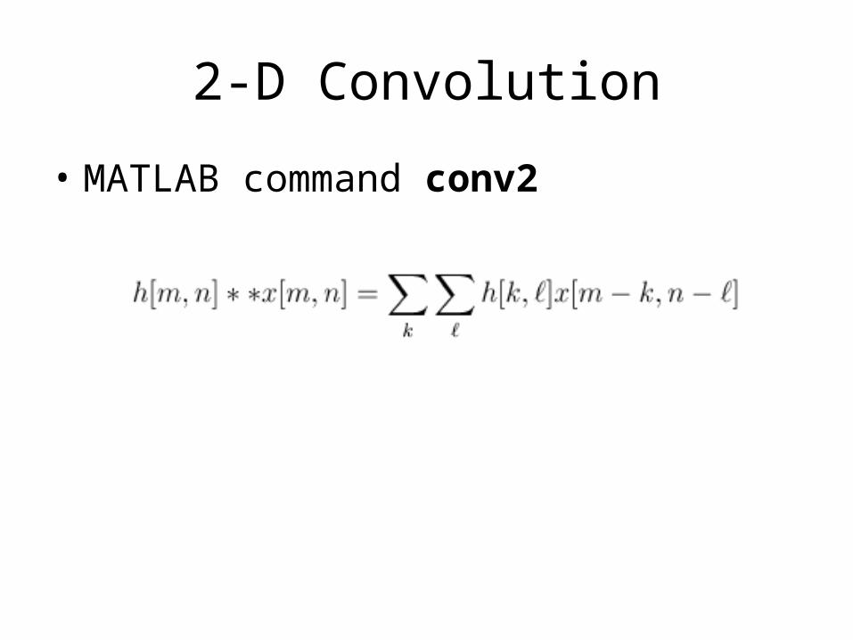
2-D Convolution
• MATLAB command conv2
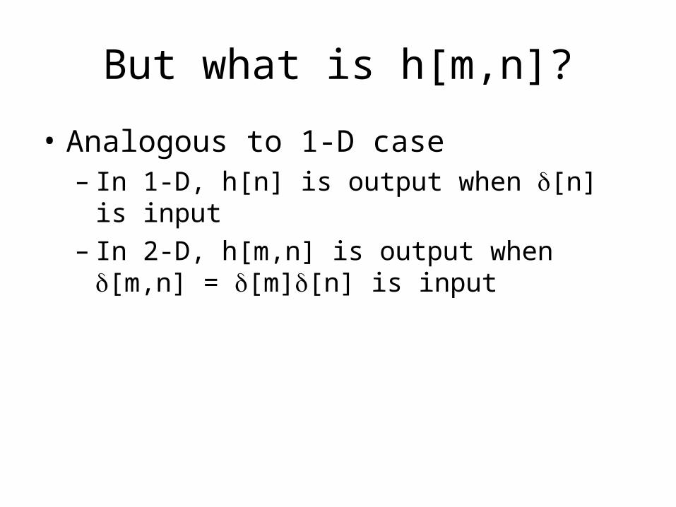
But what is h[m,n]?
• Analogous to 1-D case– In 1-D, h[n] is output when [n] is input– In 2-D, h[m,n] is output when
[m,n] = [m][n] is input
fspecial
• MATLAB command to generate some common 2-D filters (aka kernels)– Gaussian– Sobel– Prewitt
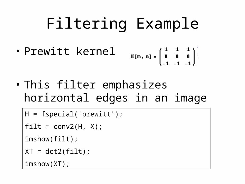
Filtering Example
• Prewitt kernel
• This filter emphasizes horizontal edges in an image
H = fspecial('prewitt');
filt = conv2(H, X);
imshow(filt);
XT = dct2(filt);
imshow(XT);
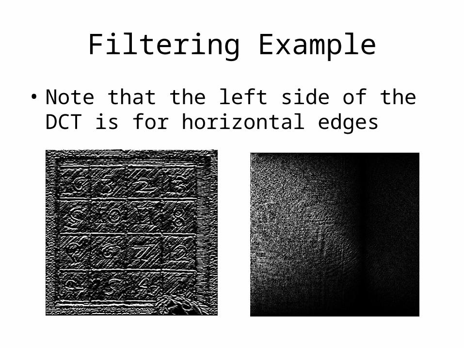
Filtering Example
• Note that the left side of the DCT is for horizontal edges
Thresholding
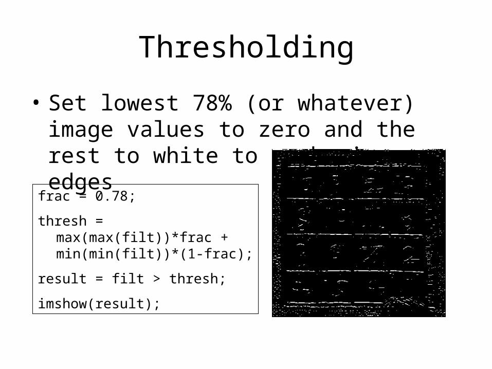
frac = 0.78;
thresh = max(max(filt))*frac + min(min(filt))*(1-frac);
result = filt > thresh;
imshow(result);
• Set lowest 78% (or whatever) image values to zero and the rest to white to emphasize edges
Recommended