General rights Copyright and moral rights for the publications made accessible in the public portal are retained by the authors and/or other copyright owners and it is a condition of accessing publications that users recognise and abide by the legal requirements associated with these rights.
Users may download and print one copy of any publication from the public portal for the purpose of private study or research.
You may not further distribute the material or use it for any profit-making activity or commercial gain
You may freely distribute the URL identifying the publication in the public portal If you believe that this document breaches copyright please contact us providing details, and we will remove access to the work immediately and investigate your claim.
Downloaded from orbit.dtu.dk on: Mar 12, 2020
FBG_SiMul V1.0: Fibre Bragg grating signal simulation tool for finite element methodmodels
Pereira, Gilmar Ferreira; McGugan, Malcolm; Mikkelsen, Lars Pilgaard
Published in:SoftwareX
Link to article, DOI:10.1016/j.softx.2016.08.001
Publication date:2016
Document VersionPeer reviewed version
Link back to DTU Orbit
Citation (APA):Pereira, G. F., McGugan, M., & Mikkelsen, L. P. (2016). FBG_SiMul V1.0: Fibre Bragg grating signal simulationtool for finite element method models. SoftwareX. https://doi.org/10.1016/j.softx.2016.08.001
FBG SiMul V1.0: Fibre Bragg Grating Signal
Simulation Tool for Finite Element Method Models
G. Pereiraa, M. McGugana, L. P. Mikkelsena
aTechnical University of Denmark, Department of Wind Energy, Frederiksborgvej 399,4000 Roskilde
Abstract
FBG SiMul V1.0 is a tool to study and design the implementation of fi-bre Bragg grating (FBG) sensors into any kind of structure or application.The software removes the need of an fibre optic expert user, becoming moreobvious the sensor response of a structural health monitoring solution usingFBG sensors. The software uses a modified T-Matrix method to simulate theFBG reflected spectrum based on the stress and strain from a finite elementmethod model. The article describes the theory and algorithm implementa-tion, followed by an empirical validation.
Keywords: Fibre Bragg Grating, Sensor Simulation in FEM, StructuralHealth Monitoring, Sensor Implementation and Optimization
1. Introduction1
More demanding structural applications and new design philosophies are2
increasingly motivating engineers and researchers to implement sensors into3
structures and to develop new structural health monitoring (SHM) solutions4
[1, 2]. This opportunity is driven by new low-cost sensors and transducers,5
new electronics and new manufacturing techniques. In particular, the cost6
of fibre Bragg grating (FBG) sensors has dropped over the last few years7
and robust fibre-optic monitoring systems suitable for SHM have become8
commercial off the shelf hardware.9
Email address: [email protected] (G. Pereira)
Preprint submitted to SoftwareX March 18, 2016

However, the sustainment of structures using these permanent on-board10
health monitoring systems is a complex and multi-disciplinary technological11
field that requires a holistic approach that cannot be addressed solely by ad-12
vances in the various technology platforms on which the SHM is constructed.13
What is required is twofold; that the next generation of research scientists14
and engineers are specifically trained with the skills, research experience,15
and multi-disciplinary background to adopt the new structural sustainment16
concepts. And that tools are available that enable the demanding task of17
integrating, supporting, and maintaining an innovative holistic health man-18
agement system and to propel its application in the aerospace, wind energy,19
and other industries.20
21
The FBG SiMul software described here is an example of the type of22
tool that will allow sensor simulation to become part of the design process,23
where output is simulated and optimised to a structure. This will have24
an immediate impact on the planning, development and implementation of25
SHM as well as provoking further research and development to include active26
control elements in the software and real-time data-driven feedback control27
for smart structures in the future. Equally important is that the software is28
robust and runs from a user friendly interface. This ensures its uptake both29
within and outside the modelling and sensor communities as it provides an30
opportunity for non-experts to simulate the signals and support their sensor31
implementation plans; whether for a one-off full-scale structural test, or a32
series of mechanical test specimens [3].33
2. Problems and Background34
The shape and response of the FBG reflected spectrum (measured signal)35
depends on the way that the grating is deformed, i.e., the stress and strain36
field acting along the grating will define the signal response. The FBG re-37
sponse simulation based on the stress and strain state from a finite element38
method (FEM) model was only recently addressed. Hu et al.[4] developed a39
Matlab code to simulate the FBG response under non-uniform strain fields40
caused by the transverse cracking in cross-ply laminates; and in a similar41
work, Hasson el al.[5] developed a Matlab code to simulate the FBG re-42
sponse for mode-I delamination detection. However, the code developed by43
both authors is limited either by the type of FEM model or by the type44
of sensor response analysed; and, in both cases the code/algorithm for the45
2

signal simulation code is not provided.46
47
Thus, FBG SiMul was developed to tackle this gap in the FBG simulation48
field, where the FBG response is simulated independently of the structure,49
loading, or application type. As the software removes the need of a fibre50
optic expert user, the FBG sensor response of a structural health monitoring51
solution becomes more intuitive.52
2.1. Fibre Bragg Grating Signal Response53
A FBG sensor is formed by a permanent periodic modulation of the re-54
fractive index along its core. When the optical fibre is illuminated by a55
broadband light source a narrow wavelength band is reflected back, as shown56
in figure 1.57
Figure 1: Fibre Bragg grating response for uniform strain, transverse stress and non-uniform strain.
Any external force/load acting in the grating region will change the effec-58
tive index and/or the period of modulation, which will create a shift in the59
wavelength and/or modify the shape of the reflected peak. However, differ-60
ent stress and strain fields acting in the FBG sensor create different signal61
responses [3, 11, 12, 13, 14] (see figure 1); a longitudinal uniform strain field62
creates a wavelength shift in the reflected peak (∆λ), but its shape remains63
unchanged; a longitudinal uniform and non-uniform strain field, acting along64
the grating, causes an increase in the reflected peak width (∆λWV ) and a65
wavelength shift (∆λ); a transverse stress field, acting along the grating,66
causes a separation of the reflected Bragg peak due to the optical fibre bire-67
fringent behaviour, which can be described by an increase in the reflected68
peak width (∆λWV ) and a wavelength shift (∆λ).69
3

2.2. Spectrum Simulation: Transfer-Matrix Method70
The transfer-matrix method was originally developed to simulate the re-71
flected spectrum of FBG sensors under a uniform strain field by Yamada and72
Sakuda [6]; later, this theory was modified to simulate the reflected spectrum73
of FBG sensors under other types of strain field or different FBG configu-74
rations [7, 8, 9, 10]. The modified T-Matrix method, developed by Peters75
et al.[7], consists of dividing the waveguides (grating periodic pattern) into76
short segments, and in each segment the grating is assumed to be periodic.77
This assumption allows each segment to be handled as a uniform grating and78
its signal to be simulated by the original Yamada T-Matrix method. Then,79
when the grating is deformed, the grating period (Λ) in each increment is80
calculated using the average strain acting in that increment; and, the total81
reflected signal is reconstructed by combining the signal contribution from82
all increments.83
2.3. From a Finite Element Method Model to Spectrum Simulation84
In a FEM model the structure domain is divided in small sections called85
elements, which contain stress and strain information that describes the86
structural behaviour. In the T-Matrix method the grating is divided into87
short segments, and the simulated signal from each segment is added to the88
total reflected signal. Thus, it is possible to simulate the FBG reflected spec-89
trum based on a FEM model, by matching the number of short segments used90
by the T-Matrix method with the number of elements in the FEM model, as91
shown in figure 2.
Figure 2: Schematic representation of the algorithm implemented in the FBG SiMul soft-ware: from a FEM model to FBG spectrum simulation;
4

92
Then, the stress and strain from each FEM element is used by FBG SiMul93
to simulate the sensor signal, using a modified T-Matrix method. The differnt94
theory and algorithm structure implemented in the software are presented in95
appendix A- Spectrum Simulation Theory and Algorithm.96
3. Software Description97
FBG SiMul was developed with a graphical user-interface, no program-98
ming knowledge is required to preform FBG simulation; all the input param-99
eters are pre-checked by the software, meaning that the simulation is robust100
and the code does not crash. However, the source code (python) is provided101
and it can be re-used or changed to fit any purpose. The software is provided102
in two formats: a standalone file, in .exe format, which does not require in-103
stallation or any dedicated software; and, in Python format, which can be104
modified but requires a python compiler.105
106
A user-manual is provided together with the software; In this documen-107
tation the user can find information about the code structure, the type of108
functions/algorithms implemented, the software input/output and different109
functionalities, and a software tutorial case.110
3.1. Software Conceptual Structure111
The FBG SiMul conceptual structure is shown in figure 3. First, the soft-112
ware extracts the stress and strain along a predefined path in a FEM model,113
and save it as a .txt file. This can be made for a specific/single time incre-114
ment, or for multiple time increments (ex: dynamic models, time dependent115
behaviour). Next, the software identifies the elements that are inside of each116
FBG, and creates a local variable per FBG sensor containing all information117
needed to simulate the FBG response, as the number of elements per grating,118
and the stress and strain field. Finally, two simulation options are given to119
the user: reflected spectrum simulation for a specific time increment, to eval-120
uate the shape of the reflected signal; and, FBG time response, to simulate121
the sensor response for multiple time increments.122
5

Figure 3: FBG SiMul conceptual structure. FBG spectrum simulation from a finite ele-ment method.
3.2. Software Functionalities123
The software is divided between 4 tabs according to functionality:124
• Tab 1- Software: Software front page, where the user can find infor-125
mation about all the different tabs and their functionalities, open the126
user manual, or learn more about the software copyright and author;127
• Tab 2- Extract Stress/Strain along Optical Fibre (Abaqus):128
Tool to automatically extract the stress and strain along a pre-defined129
path in a FEM model. The output is a .txt file containing the stress130
and strain distribution along a FBG path for a specific time increment.131
Tool options: multiple FBG paths; coordinate system rotation; single132
or multiple time increment;133
6

Note: this tool was developed for Abaqus FEM models. Nevertheless,134
the user can simulate the FBG response using a different FEM software135
by extracting the files manually, and ensuring that the files have the136
required format, as described in the user-manual.137
• Tab 3- FBG Spectrum Simulation (Specific Step Increment):138
FBG reflected spectrum simulation for a specific time increment. Here,139
the user can study the FBG spectrum response, plan the sensor loca-140
tion, optimise the sensor wavelength, check available bandwidth, eval-141
uate signal distortion or measurement errors, and so forth. The tab142
output is the FBG reflected spectrum, and it can be saved as an im-143
age or as a .txt file. Tool options: different SI units, mm or m; type144
of simulation, as longitudinal uniform strain, longitudinal non-uniform145
strain or transverse stress; user-defined optical fibre parameters; num-146
ber of FBG sensors per fibre; FBG length; user-defined FBG array147
configuration; plot configuration;148
• Tab 4- FBG Signal variation (Time Response): FBG signal re-149
sponse for multiple time increments. Here, the user can study the150
wavelength shift variation(∆λWV ) and the peak width variation (∆λ)151
along the selected time increments, compare the sensor response for152
multiple FBG paths, plan the sensor location, and so forth. The tab153
output is the ∆λWV and ∆λ along the selected time increments, and154
it can be saved as an image or as a .txt file. Tool options: different SI155
units, mm or m; user-defined optical fibre parameters; number of FBG156
sensors per fibre; FBG length; user-defined FBG array configuration;157
plot configuration;158
4. Software Empirical Validation159
To validate the software algorithm, 3 input files representing known cases160
of uniform strain, non-uniform strain and transverse stress were created. The161
wavelength shift, ∆λWV , and the peak width variation, ∆λ, for the 3 cases162
were calculated using the analytical equations (Eq. (3), (7), and (11)) de-163
veloped by Pereira et al. [3]. Each input file contains the stress and strain164
along a 10 mm grating, discretized in 20 segments.165
166
7

Theoretical results:167
• Uniform strain: grating under 1.0 ε(%) longitudinal strain. Theoretical168
output: ∆λ = 12.16 nm, ∆λWV = 0; for pe = 0.215 and λb = 1550 nm.169
• Non-uniform strain: half grating under 1.0 ε(%) and the other half170
under 0.5 ε(%) longitudinal strain. Theoretical output: ∆λ = 9.15nm,171
∆λWV = 6.07 nm; for pe = 0.215, λb = 1550 nm, neff = 1.46 and172
Λ0 = 530.82.173
• Transverse stress: grating under a compressive stress of 100MPa in174
the z direction. Theoretical output: ∆λ = 0 nm, ∆λWV = 0.3839 nm;175
for p11 = 0.121, p12 = 0.270, E = 70 GPa, ν = 0.17, λb = 1550 nm,176
neff = 1.46 and Λ0 = 530.82.177
Figure 4: FBG SiMul simulation results. Simulated test cases: uniform strain, non-uniform strain, and transverse stress.
The three empirical test cases were simulated with good accuracy by the178
FBG SiMul software, as shown in figure 4. Thus, it can be concluded that the179
software can represent the FBG response for different type of strain/stress180
fields.181
5. Illustrative Example182
In this section, the FBG SiMul was used simulate and design a delami-183
nation/crack monitoring solution based in FBG sensors. A double cantilever184
beam (DCB) FEM model, based on the work presented by Pereira et al. in185
[3], was used to represent the delamination phenomenon. The complete FEM186
8

model description and a simulation tutorial can be found in the FBG SiMul187
user-manual.188
The simulated virtual FBG array was composed of 5 gratings, spaced189
by 10 mm (see figure 5), and its path was a 0.03 mm line parallel with190
the delamination plane. Then, the FBG array spectrum response in the191
presence of a crack was simulated using the FBG SiMul tab 3; and, the192
FBG signal response during the delamination process was simulated using193
the FBG SiMul tab 4.194
Figure 5: FBG array configuration in the DCB specimen.
5.1. FBG Spectrum Simulation195
The reflected spectrum was simulated for a specific time increment using196
the FBG SiMul tab 3-FBG Spectrum Simulation, where the crack tip was197
situated 36 mm from the beginning of the optical fibre, which corresponds198
to the middle of the second grating.199
A screen-shoot of the FBG SiMul plot/output window is shown in figure200
6, where the deformed reflected spectrum (red curves) can be compared with201
the original reflected spectrum (grey curves). It can be observed that the202
two first FBGs measure a high amount of wavelength shift (∆λ) and peak203
width variation (∆λWV ), as result of the presence of the crack.204
5.2. FBG Time Response Simulation205
The FBG response was simulated using the FBG SiMul tab 4-FBG Signal206
Variation. It was used multiple time increments, representing the delamina-207
tion of the DCB specimen, from an undamaged to a fully damage state. A208
9

Figure 6: FBG SiMul plot window: FBG reflected spectrum simulation for the non-uniform strain contribution.
screen-shoot of the FBG SiMul plot/output window is shown in figure 7,209
where the top plot represents the wavelength shift(∆λWV ), and the bottom210
plot represents the peak width variation (∆λ). This simulation shows an211
increase of the ∆λ as the crack passes the position of the grating, caused by212
change in the material compliance and load distribution; and, an increase213
of the ∆λWV when the crack is near the grating, caused by a non-uniform214
strain field generated at the crack tip.215
10

Figure 7: FBG SiMul plot window: FBG time response simulation.
6. Conclusions216
FBG SiMul provides the user with a tool to study and design structural217
health monitoring solutions based on FBG sensors. The software is divided218
in 3 main tools: a tool to extract the stress and strain along an optical fibre219
path from a FEM model; a tool to simulate the reflected spectrum for a220
specific time increment; and a tool to simulate the FBG time response.221
222
The software uses a modified version of the T-Matrix method to simulate223
the FBG signal from a FEM model. Thus, it can simulate the FBG response224
independently of the type of structure, loading or application. Also, the225
software removes the need of a fibre optic expert to plan and design monitor-226
ing solutions. The user interacts with the software through a user-interface,227
meaning that no programming knowledge is required, making parameter ma-228
nipulation more intuitive to the user. Also, the input data is pre-checked by229
11
the software, meaning that the simulation is robust and does not crash or230
give calculation errors.231
Acknowledgements232
The author acknowledges the Seventh Framework Programme (FP7) for233
funding the project MareWint (Project reference: 309395) as Marie-Curie234
Initial Training Network.235
References236
[1] D.F.O. Braga, S.M.O. Tavares, L.F.M. da Silva, P.M.G.P. Mor-237
eira, P.M.S.T. de Castro, Advanced design for lightweight struc-238
tures: Review and prospects, Prog. Aerosp. Sci. 69 (2014) 2939.239
doi:10.1016/j.paerosci.2014.03.003.240
[2] P. Takoutsing, R. Wamkeue, M. Ouhrouche, F. Slaoui-Hasnaoui, T.241
Tameghe, G. Ekemb, Wind Turbine Condition Monitoring: State-of-242
the-Art Review, New Trends, and Future Challenges, Energies. 7 (2014)243
25952630. doi:10.3390/en7042595.244
[3] G.F. Pereira, L.P. Mikkelsen, M. McGugan, Crack Detection in Fibre245
Reinforced Plastic Structures Using Embedded Fibre Bragg Grating246
Sensors: Theory, Model Development and Experimental Validation.,247
PLoS One. 10 (2015) e0141495. doi:10.1371/journal.pone.0141495.248
[4] H. Hu, S. Li, J. Wang, Y. Wang, L. Zu, FBG-based real-time evaluation249
of transverse cracking in cross-ply laminates, Compos. Struct. 138 (2016)250
151160. doi:10.1016/j.compstruct.2015.11.037.251
[5] O. Hassoon, M. Tarfoui, a El Malk, Numerical Simulation of Fiber Bragg252
Grating Spectrum for Mode- Delamination Detection, Int. J. Mech.253
Aerospace, Ind. Mechatronics Eng. 9 (2015) 144149.254
[6] M. Yamada, K. Sakuda, Analysis of almost-periodic distributed feedback255
slab waveguides via a fundamental matrix approach., Appl. Opt. 26256
(1987) 34743478. doi:10.1364/AO.26.003474.257
12

[7] K. Peters, M. Studer, J. Botsis, A. Iocco, H. Limberger, R. Salath,258
Embedded optical fiber Bragg grating sensor in a nonuniform strain259
field: Measurements and simulations, Exp. Mech. 41 (2001) 1928.260
doi:10.1007/BF02323100.261
[8] H.-Y. Ling, K.-T. Lau, W. Jin, K.-C. Chan, Characterization of dynamic262
strain measurement using reflection spectrum from a fiber Bragg grating,263
Opt. Commun. 270 (2007) 2530. doi:10.1016/j.optcom.2006.08.032.264
[9] Y. Chen, J. Li, Y. Yang, M. Chen, J. Li, H. Luo, Numerical modeling265
and design of mid-infrared FBG with high reflectivity, Opt. - Int. J. Light266
Electron Opt. 124 (2013) 25652568. doi:10.1016/j.ijleo.2012.07.016.267
[10] A. Ikhlef, R. Hedara, M. Chikh-bled, Uniform Fiber Bragg Grating mod-268
eling and simulation used matrix transfer method, IJCSI Int. J. Comput.269
Sci. 9 (2012) 368374.270
[11] L. Bjerkan, K. Johannessen, X. Guo, Measurements of Bragg grating271
birefringence due to transverse compressive forces, Proc. 12th Interna-272
tional Conference on Optical Fiber Sensors, 16 (1997) 6063.273
[12] F. Jlich, J. Roths, Comparison of transverse load sensitivities of fibre274
Bragg gratings in different types of optical fibres, in: F. Berghmans,275
A.G. Mignani, C.A. van Hoof (Eds.), Opt. Sens. Detect., 2010: p.276
77261N. doi:10.1117/12.854019.277
[13] L. Sorensen, J. Botsis, T. Gmr, J. Cugnoni, Delamination detec-278
tion and characterisation of bridging tractions using long FBG opti-279
cal sensors, Compos. Part A Appl. Sci. Manuf. 38 (2007) 20872096.280
doi:10.1016/j.compositesa.2007.07.009.281
[14] S. Stutz, J. Cugnoni, J. Botsis, Crack fiber sensor interaction and char-282
acterization of the bridging tractions in mode I delamination, Eng. Fract.283
Mech. 78 (2011) 890900. doi:10.1016/j.engfracmech.2011.01.014.284
13
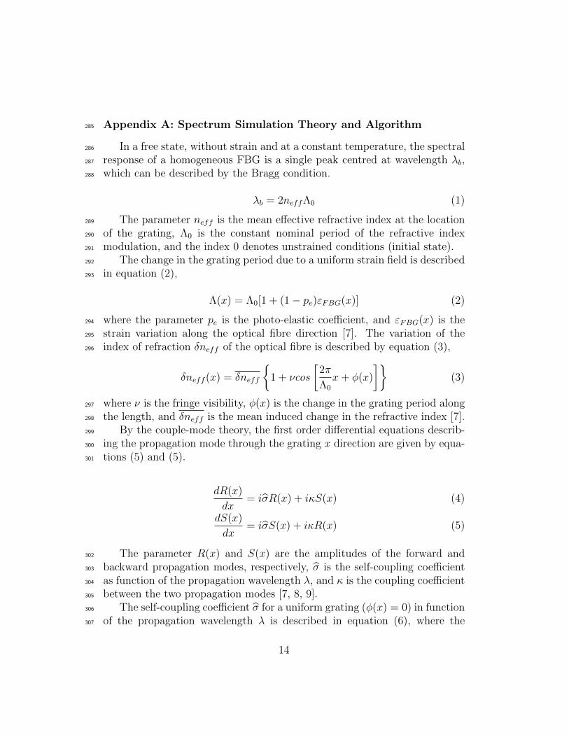
Appendix A: Spectrum Simulation Theory and Algorithm285
In a free state, without strain and at a constant temperature, the spectral286
response of a homogeneous FBG is a single peak centred at wavelength λb,287
which can be described by the Bragg condition.288
λb = 2neffΛ0 (1)
The parameter neff is the mean effective refractive index at the location289
of the grating, Λ0 is the constant nominal period of the refractive index290
modulation, and the index 0 denotes unstrained conditions (initial state).291
The change in the grating period due to a uniform strain field is described292
in equation (2),293
Λ(x) = Λ0[1 + (1− pe)εFBG(x)] (2)
where the parameter pe is the photo-elastic coefficient, and εFBG(x) is the294
strain variation along the optical fibre direction [7]. The variation of the295
index of refraction δneff of the optical fibre is described by equation (3),296
δneff (x) = δneff
{1 + νcos
[2π
Λ0
x+ φ(x)
]}(3)
where ν is the fringe visibility, φ(x) is the change in the grating period along297
the length, and δneff is the mean induced change in the refractive index [7].298
By the couple-mode theory, the first order differential equations describ-299
ing the propagation mode through the grating x direction are given by equa-300
tions (5) and (5).301
dR(x)
dx= iσ̂R(x) + iκS(x) (4)
dS(x)
dx= iσ̂S(x) + iκR(x) (5)
The parameter R(x) and S(x) are the amplitudes of the forward and302
backward propagation modes, respectively, σ̂ is the self-coupling coefficient303
as function of the propagation wavelength λ, and κ is the coupling coefficient304
between the two propagation modes [7, 8, 9].305
The self-coupling coefficient σ̂ for a uniform grating (φ(x) = 0) in function306
of the propagation wavelength λ is described in equation (6), where the307
14

parameter λb is the FBG reflected wavelength in an unstrained state defined308
by the equation (1).309
σ̂ = 2πneff
(1
λ− 1
λb
)+
2π
λδneff (6)
The coupling coefficient between the two propagation modes κ is defined310
by equation (7), where the parameter m is the striate visibility that is ≈ 1311
for the conventional single mode FBG [8, 9].312
κ =π
λmδneff (7)
Spectrum reconstruction313
314
The optical response matrix of the ith (each segment) uniform grating315
can be described by the coupled mode theory [4, 8]. By considering the FBG316
length (L) divided in n short segments, then the ∆x = L/n is the length317
of each segment. Note that n is constrained by the grating period [8], as318
described by equation (8).319
n ≤ 2neff
λbL (8)
For the FBG length limits, −L/2 ≤ x ≥ L/2, and the boundary condi-320
tions, R(−L/2) = 1 and S(L/2) = 0, the solution of the coupling mode of321
equations (5) and (5) can be expressed as:322 [R(xi+1)
S(xi+1)
]= Fxi,xi+1
[R(xi)
S(xi)
](9)
where R(zi) and S(zi) are the input light wave travelling in the positive323
and negative directions, respectively, and R(zi+1) and S(zi+1) are the output324
waves in the positive and negative directions, respectively. Thus, the TTM325
matrix Fxi,xi+1for each segment (∆x) of the grating can be calculated using326
the equation (10) and (11).327
Fxi,xi+1=
[S11 S12
S21 S22
](10)
15
S11 = cosh(γB∆x)− i σ̂γBsinh(γB∆x)
S12 = −i κγBsinh(γB∆x)
S21 = iκ
γBsinh(γB∆x)
S22 = cosh(γB∆x) + iσ̂
γBsinh(γB∆x)
γB =√κ2 − σ̂2
(11)
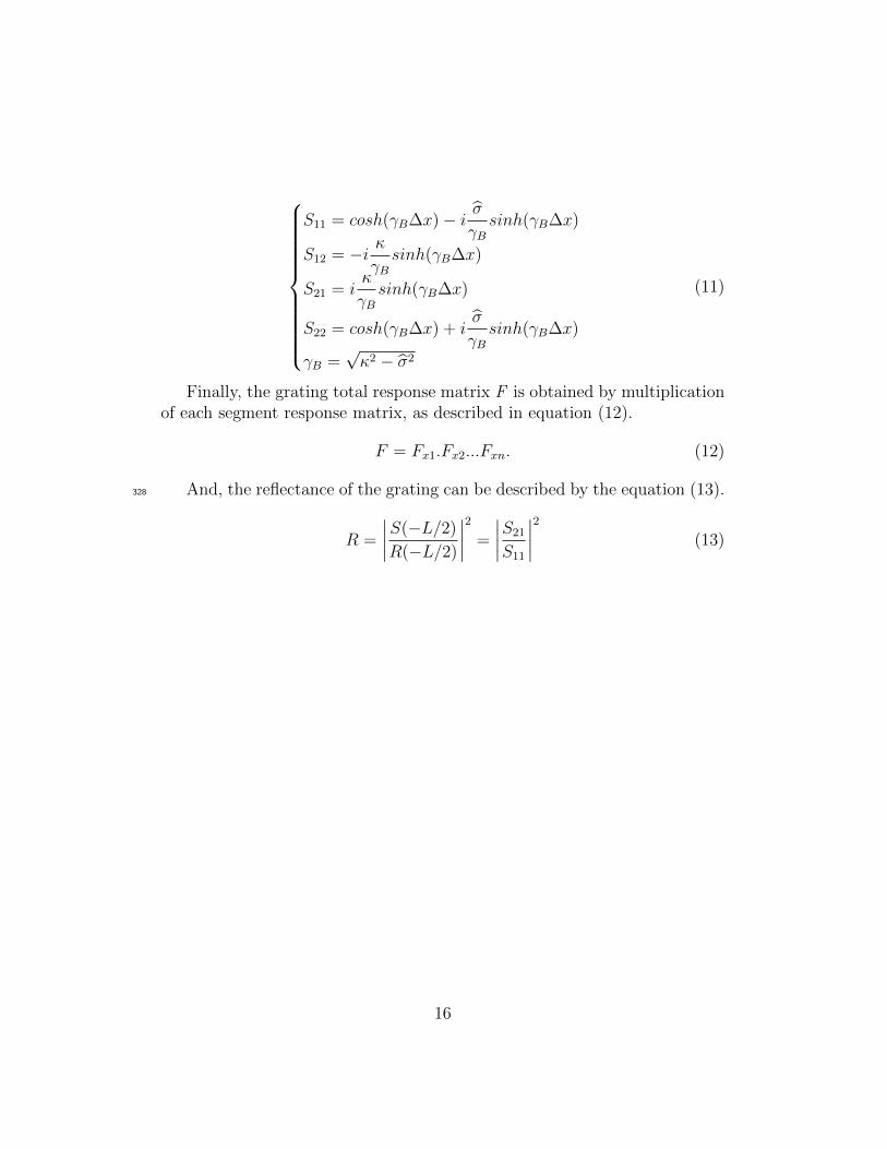
Finally, the grating total response matrix F is obtained by multiplicationof each segment response matrix, as described in equation (12).
F = Fx1.Fx2...Fxn. (12)
And, the reflectance of the grating can be described by the equation (13).328
R =
∣∣∣∣S(−L/2)
R(−L/2)
∣∣∣∣2 =
∣∣∣∣S21
S11
∣∣∣∣2 (13)
16

FBG SiMul spectrum simulation algorithm structure329
330
The structure of the spectrum simulation algorithm implemented in the331
FBG SiMul is shown in figure 8.332
Figure 8: FBG SiMul spectrum simulation algorithm structure.
17

Required Metadata333
Current executable software version334
Nr. (executable) Software metadatadescription
Please fill in this column
S1 Current software version V1.0S2 Permanent link to executables of
this versionhttps://github.com/GilmarPereira/FBG SiMul.git
S3 Legal Software License GNU GPL-3S4 Computing platform/ Operating
SystemWindows;
S5 Installation requirements & depen-dencies
None for standalone file; Python2.7.5 for Python format;
S6 If available, link to user manual - ifformally published include a refer-ence to the publication in the refer-ence list
https://github.com/GilmarPereira/FBG SiMul/blob/master/Standalone Version/Software Documentation.pdf
S7 Support email for questions [email protected];gilmar [email protected];
Table 1: Software metadata (optional)
18
Recommended