Proceedings of GPPS Forum 18 Global Power and Propulsion Society
Zurich, 10th-12th January 2018 www.gpps.global
© 2018 by General Electric Technology GmbH. All right reserved. Information contained in this document is indicative only. No representation or warranty is given
or should be relied on that it is complete or correct or will apply to any particular project. This will depend on the technical and commercial circumstances. It is
provided without liability and is subject to change without notice. Reproduction, use or disclosure to third parties, without express written authority, is strictly
prohibited.
GPPS-2018-0048
FAST NUMERICAL CALCULATION APPROACHES FOR THE MODELLING OF TRANSIENT TEMPERATURE FIELDS IN A STEAM TURBINE IN PRE-WARMING OPERATION WITH HOT AIR
Piotr Łuczyński RWTH Aachen
[email protected] Aachen, Germany
David Erdmann RWTH Aachen
[email protected] Aachen, Germany
Dennis Többen RWTH Aachen
[email protected] Aachen, Germany
Manfred Wirsum RWTH Aachen
[email protected] Aachen, Germany
Klaus Helbig GE Power AG
[email protected] Mannheim, Germany
Wolfgang Mohr GE Power AG
[email protected] Baden, Switzerland
ABSTRACT
Recently, the reduction of steam turbine start-up times has
become increasingly important. In pursuit of this objective,
General Electric has developed a concept for both the pre-
warming and warm-keeping of steam turbines with hot air. To
investigate the thermally induced stresses, a computationally
efficient method is required for the simulation of transient
temperature distribution in the turbine during pre-warming. In the
presented work, four transient calculation methods are
investigated for pre-warming simulation. Firstly, a modified
Frozen Flow method is used in order to conduct transient
conjugate heat transfer (CHT) simulations. Secondly, two
uncoupled approaches called TFEA-LINR and the TFEA-EXPO
are applied to calculate heat transfer coefficients from steady-
state calculations. In addition, a fourth approach called the
Equalized Timescales (ET) method is presented. In this CHT
method, the specific heat capacity of the solid state is reduced by
a “speed up factor” to reduce transient heating time.
1. INTRODUCTION
The situation of the European energy market is evolving
dynamically. The greatest challenge engineers have to face in the
field of successful integration of renewable energy sources with
existing power systems is a variability and certain
unpredictability of electricity generation from wind or solar
energy sources.
The flexibility and load gradients of coal-fired power plants
in particular must be increased for both economic reasons, and in
order to ensure a balance between total generation and
consumption of power in real time. The typical start-up time of a
conventional power unit (over 500 MWth) from cold state is
estimated to be about five to eight hours (Vogt et al., 2013), and
is influenced by high values of thermal stresses induced in the
thick-walled HP and IP steam turbine components. Steeper load
gradients during the frequent start-ups of a conventional power
plant unavoidably lead to higher thermal stresses and, from a
lifetime assessment point of view, increase the probability of
crack development. Hence, a reduction in the start-up time with
an unaffected turbine lifetime consumption requires innovative
technical solutions.
A possible solution to achieve a reduction of thermal stresses
during start-up is the concept of turbine warm-keeping, or pre-
warming. The warm-keeping methods focus on minimizing or
compensating for heat losses that occur during periods of turbine
inactivity and, in contrast to pre-warming operations, do not
require arduous turbine heating from cold states.
The concept of warm-keeping or pre-warming of steam
turbines with hot air (depending on the initial thermal boundary
conditions) was presented by Helbig et al. (2014). In the proposed
technical arrangement, the rotating turbine is heated by circulated
hot air. The first investigation of warm-keeping operations
concerning fluid field as well as heat transfer phenomena (based
on the concept developed by Helbig et al. (2014)) was given by
Toebben et al. (2017). This research is based on steady state
calculation approaches. In the next step presented in this work,
the numerical methods allowing unsteady simulation of pre-
warming operations are investigated.
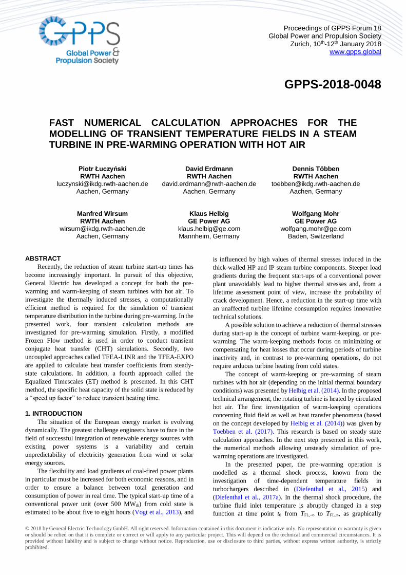
In the presented paper, the pre-warming operation is
modelled as a thermal shock process, known from the
investigation of time-dependent temperature fields in
turbochargers described in (Diefenthal et al., 2015) and
(Diefenthal et al., 2017a). In the thermal shock procedure, the
turbine fluid inlet temperature is abruptly changed in a step
function at time point t0 from TFL,-∞ to TFL,∞, as graphically
2
depicted in Figure 1. The resulting logarithmic growth of solid
body temperatures in pre-warming processes is situated between
cold turbine state at operating point 1 (OP1) and warm-keeping
operation at operating point 2 (OP2). Thus, due to the intense heat
exchange between cold turbine components and hot working
fluid, especially at the first phase of the pre-warming procedure,
higher temperature gradients are expected as in warm-keeping
operation. The main objective of the research presented in this
paper is the development of a fast and generally valid method for
the calculation of the transient temperature fields in turbine pre-
warming, with regards to thermomechanical fatigue. In order to
achieve this goal, several unsteady calculation approaches known
from literature are implemented into numerical models of pre-
warmed steam turbines. Of particular interest are the numerical
methods that enable the bridging of the gap between vastly
different time scales of solid and fluid states.
Figure 1 Behavior of fluid and solid temperatures in pre-warming and warm-keeping operation
In the following section (Sec. 2), the numerical models used
for steady and transient calculations are presented. Subsequently,
the unsteady simulation approaches allowing the calculation of
transient temperature fields in fluid and solid states are discussed
(Sec. 3). The comparison of the results obtained using the chosen
simulation methods is provided in the penultimate section
(Sec. 4), just before the conclusion (Sec. 5).
2. NUMERICAL MODEL
In cooperation with the industrial partner General Electric, a
numerical model of a single repeating turbine stage has been
developed. For pre-warming calculation purposes, the numerical
model for warm-keeping operation, known from research
presented by Toebben et al. (2017), is used, and hence, only the
most relevant information concerning model setup and changes
introduced to original settings are provided. Due to the high live
steam turbine temperature, the thermally induced stresses arise
particularly within the first turbine stage. Thus, the investigation
of heat transfer and calculation approaches focuses on a single
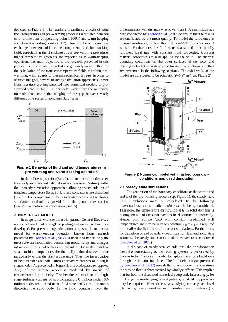
stage model. As presented in Figure 2, one blade passage (approx.
2.5°) of the turbine wheel is modelled by means of
circumferential periodicity. The hexahedral mesh of all single
stage turbines consists of approximately 6.8 million nodes. 3.6
million nodes are located in the fluid state and 3.1 million nodes
discretize the solid body. In the fluid boundary layer the
dimensionless wall distance y+ is lower than 1. A mesh study has
been conducted by Toebben et al. (2017) to ensure that the results
are unaffected by the mesh quality. To model the turbulence in
thermal sub-layers, the low Reynolds kω-SST turbulence model
is used. Furthermore, the fluid state is assumed to be a fully
turbulent ideal gas with constant fluid properties. Constant
material properties are also applied for the solid. The thermal
boundary conditions on the outer surfaces of the rotor and
housing differ between steady and transient simulations, and thus
are presented in the following sections. The axial walls of the
model are considered to be adiabatic (q̇=0 W m-2, cp. Figure 2).
Figure 2 Numerical model with marked boundary conditions and used denotation
2.1 Steady state simulations
For generation of the boundary conditions at the start t0 and
end t∞ of the pre-warming process (cp. Figure 1), the steady state
CHT simulations must be calculated. In the following
investigations, the so called cold start is being considered.
Therefore, the temperature distribution at t0 in solid domains is
homogenous and does not have to be determined numerically.
Hence, only simple CFD with constant predefined wall
temperatures and turbine inlet temperature TTI = TFL,∞ is required
to initialise the fluid field of transient simulations. Furthermore,
for definition of end boundary conditions for fluid and solid state
at time t∞, the steady state CHT calculations have to be conducted
(Toebben et al., 2017).
In the case of steady state calculations, the transformation
from the non-rotating to the rotating system is performed by
Frozen Rotor Interface, in order to capture the strong backflows
through the domains interfaces. The fluid field analysis presented
by Toebben et al. (2017) reveals that in warm-keeping operations
the turbine flow is characterized by windage effects. This implies
that for both the discussed numerical setup and, interestingly, for
multistage warm-keeping investigations, unsteady approaches
may be required. Nevertheless, a satisfying convergence level
(defined by presupposed values of residuals and imbalances) in

3
single stage simulations is achieved by a low value of timescale
applied to fluid domains, which result in under-relaxation of
governing equations.
Moreover, the missing thermal boundary conditions for rotor
and housing are defined as follows: surfaces of the predefined
concentric hole in the rotor, and the outer surfaces of the inner
steam turbine casing, are represented by TR and TH respectively
(cp. Figure 2). The temperature values amount to approximately
45% of the live steam temperature at nominal load.
2.2 Transient simulations
The pre-warming operation presented in this work is
modelled as a thermal shock process. Therefore, corresponding
with previously described assumptions of the thermal shock
procedure, the turbine inlet temperature TTI in pre-warming
operation is considered to be constant and equal to TFL,∞. As a
result of this assumption, the numerically determined temperature
gradients in turbine components can be overestimated, especially
at the beginning of the thermal shock process. Nevertheless, the
chosen modelling approach allows the identification of critical
zones in a pre-warmed steam turbine where, due to the varying
heat exchange conditions in the flow channel, high thermally
induced stresses occur.
The temperatures on the outer surfaces of the rotor
TR = T(q̇Rotor) and housing TH = T(q ̇Housing) (cp. Figure 2) are defined
based on the values of heat flux obtained from steady state
calculations. At the end of pre-warming procedure - time point t∞
- the boundary conditions correspond to the boundary conditions
of warm-keeping operation. Therefore, some of the
aforementioned considerations analysing unsteady numerical
approaches can additionally be used to investigate the warm-
keeping operation (cp. Figure 2, OP2).
3 MODELING OF HEAT TRANSFER
The key issue in the assessment of turbine lifetime
consumption, as well as in the determination of
thermomechanical fatigue caused by high thermally induced
stresses, is the modelling of heat exchange between fluid flow and
solid bodies with sufficient accuracy. Two main calculation
approaches can be distinguished in literature. In the coupled
method, also known as the conjugate heat transfer approach
(CHT), a CFD simulation is iteratively coupled with a conductive
finite element analysis (FEA). The solution of the energy
equation at the coupled boundaries ensures the continuity of the
heat fluxes and temperature fields on the fluid/solid interfaces.
The description of the investigation of employed CHT approach
is given at (Bohn et al., 2003), and its technical implementation
into the model of a turbocharger can be found at (Bohn et al.,
2005).
In contrast to CHT methods, most of the uncoupled
approaches are based on the assumption of constant heat transfer
coefficients (HTC) on boundary interfaces, implying a linear
relation between the convective heat fluxes across the fluid/solid
interface and the driving temperature differences. The HTC
values obtained by the CFD calculation are used in the subsequent
step for FEA calculation. Although the uncoupled methods may
lead to inaccuracies caused by locally nonlinear plots of HTC, a
significant reduction of computational time can be achieved.
Examples of these methods in the context of rotor-stator cavities
investigation are given by Alizadeh et al. (2007) as well as Lewis
and Provins (2004).
The main challenge unsteady coupled calculation
approaches face are the vastly different time scales of the
convective and the conductive heat transfer in fluid and solid
states, as reported by He and Oldfield (2011). Therefore, the CHT
methods are usually applied to steady state simulations, and their
implementation into time accurate calculations requires
additional assumptions.
In this work, four numerical methods – Frozen Flow (FF),
TFEA-EXPO, TFEA-LINR and Equalized Timescales (ET) – are
employed in order to calculate the heat transfer in pre-warming
operations. Furthermore, some of the presented calculation
approaches are successfully utilized by Diefenthal et al. (2017a)
for modelling of heat transfer in commercial vehicle
turbochargers. The fluid field in the turbine wheel of the
considered turbocharger is characterized by values of Re-number
between 7*105-2.7*106 (depending on the operating point), and
Pr-number of about 0.57-0.7. The heat transfer on a turbine wheel
is described by Nu-numbers, the values of which vary between 61
and 204 in stationary operation. Interestingly, the numerical
simulations of the pre-warming turbine operation reveal Re-
numbers of about 5.0*105 (value is strongly dependent on the
mass flow rate), Pr-number equal to 0.72 and Nu-numbers on
blade surfaces of about 67-100. Furthermore, as the concept of
pre-warming of steam turbines with hot air is an innovative
approach, there are still no validation data provided. Hence, due
to the similar heat transfer conditions in the numerical models of
both turbomachines, the modified reference simulation method of
turbocharger investigations (known as Frozen Flow method) is
also considered as a reference approach for pre-warming
calculations. The difference between the original FF method
(named as “FF transient update”) and modified FF approach (“FF
stationary update”) newly presented in this work, is the way of
“updating” the fluid field. In order to ensure that the introduced
changes to the FF method (which result in additional
computational time savings) do not significantly affect the
accuracy of the original simulation approach, in the first step the
FF stationary update method is validated on the model of the
turbocharger. In the second step, the validated FF stationary
update is used as a reference approach for pre-warming
calculations. A detailed description of both the FF methods and
validation of the FF stationary update approach on the model of
the turbocharger is given in Sec. 3.1. Moreover, based on the FF
results, the position of investigation points P1 and P2, in which
the highest temperature gradients in pre-warming operation
occur, is determined (cp. Figure 2). In the following sections, both
points located on vane and blade surfaces are used to compare
analysed simulation methods.
In the next step, the two methods belonging to the family of
uncoupled heat exchange simulation approaches are investigated.
In the first uncoupled approach model, the heat transfer
coefficients demonstrate exponential behaviour in the thermal
shock procedure and, hence, it is called a transient finite element
analysis method-exponential (TFEA-EXPO). The TFEA-EXPO
calculation approach has been developed by Diefenthal et al.
(2015) based on another uncoupled method, which enables

4
determination of transient temperature fields in solid state by
means of linear interpolation of HTCs over a specified time
period. Therefore, the second uncoupled approach is abbreviated
as TFEA-LINR. Both TFEA methods are discussed in Sec. 3.2.
The fourth and final method achieves a significant
computational time reduction by modification of material
properties of solid state, and thus equalization of fluid and solid
time scales. Hence, this approach – which is already used for
unsteady investigations of turbochargers (Diefenthal et al.,
2017a; Diefenthal et al., 2017b) – is referred to as the Equalized
Timescales method. This approach does not employ any
assumptions concerning fluid state (like FF method), and allows
coupled simulation over the whole transient process. A more
detailed description of ET approach follows in Sec. 3.3.
3.1 FF method
In order to overcome the extremely high computational times
in unsteady CHT calculations, it is assumed in the first method
that the pressure and velocity distribution of the fluid field remain
constant over certain periods of time. Hence, corresponding to
this assumption, the mass, momentum and turbulence equations
of the fluid state are not solved and consequently, larger time
steps can be used. Obviously, this assumption leads to
inaccuracies in solutions, especially in the first phase of the
thermal shock process, mainly due to the intense heat transfer
over the fluid/solid interfaces. In the FF approach originally
developed for investigations of turbochargers presented by Heuer
et al. (2006), no further precautions have been taken for
enhancement of calculation accuracy. An improved accuracy of
the discussed method has been achieved by introducing additional
CHT simulations, in which all equations (mass, momentum and
turbulence) are solved at the predefined time points of transient
processes and the “update” of fluid field occurs (Diefenthal et al.,
2015). The adjustment of velocity and pressure distribution to
transient temperature fields may also be realized by replacing the
fully unsteady CHT calculations with simple stationary CFD
simulations. In the following, the second possibility of the fluid
field update is investigated and in the first step it is applied to the
turbocharger model described by Diefenthal et al. (2015) for
validation purposes. Subsequently, the CFD update based FF
method is employed to determine the heat exchange and flow
field in a pre-warmed steam turbine.
The main goals of the experimental and numerical
investigations conducted for commercial vehicle turbochargers
were similar to the pre-warming objectives, as the turbocharger
analysis focused on the capturing of transient temperature fields
in the context of thermomechanical fatigue. The numerical model
of a turbocharger with its main components including inlet/outlet
pipes, volute and turbine wheel is shown in Figure 3.
The turbine wheel of the turbocharger is established as a
single rotor passage based on the mixing plane assumption
between stationary and rotating domains. The boundary
conditions on the shaft, including heat fluxes to the gas, lubricant
oil and to compressor side, are defined by means of heat transfer
coefficients α1, α2 (with reference temperatures Tref,1, Tref,2) and
heat flux q̇. Similar to the steam turbine simulations, the low
Reynolds kω-SST turbulence model is used to calculate the flow
field and heat transfer on the 6.2 million nodes mesh with
dimensionless wall distance y+ lower than 1. In the case of
turbocharger investigations, the thermal shock process is also
Figure 3 Numerical model of turbine housing (TH) and turbine wheel (TW)
considered, with the fluid flow temperatures TFL being abruptly
changed from TFL,-∞ = 200°C to TFL,∞ = 600°C. During the entire
thermal shock procedure, the temperature values at the
measurement points presented in Figure 4 are recorded. More
detailed information concerning experimental as well as
numerical setup may be found at (Diefenthal et al., 2015) and
(Diefenthal et al., 2017a).
In the original FF method applied to the turbocharger, the
fully transient CHT updates are conducted at 0s, 6s and 60s of the
thermal shock process (cp. Diefenthal et al., 2015). In the
presented work, the second, previously mentioned approach
based on the CFD update simulation is analysed.
Figure 4 Position of measurement points on turbine wheel
The stationary CFD update simulation procedure of the
thermal shock is given in Figure 5. At the beginning of the
simulation process, a conventional steady state CFD or CHT
calculation is conducted for initialisation of fluid field and
eventually, temperature distribution in solid state. After providing
the necessary start conditions, the time-marching CHT
calculation solving only energy equations (“Only Energy”
period) is performed. The determined temperatures on the flow
channel walls are used in steady state CFD update simulations as
boundary conditions, in order to achieve the adjustment of
pressure and velocity flow fields with regards to changing energy
content. The fluid field obtained in CFD, together with the solid-
state temperature distribution known from the last time point of
the previous Only Energy CHT calculation, are sufficient for
initialisation of the next Only Energy transient period. The

5
described procedure may be repeated for any required number of
update calculations. In contrast to the original FF approach, the
fully transient CHT periods are replaced with steady state CFDs.
Hence, in the discussed turbocharger model, the computational
time is decreased by a factor of 40 in reference to the fully
transient update method. This result is of particular importance,
especially in the case of simulations of long processes (like pre-
Figure 5 Stationary CFD update simulation procedure
warming), which may be characterized by a higher number of
required update calculations.
The heat exchange between fluid and solid in the operation
of turbochargers is mainly characterized by convective heat
transfer. Therefore, the impact of the updates on the fluid field in
the turbine wheel is evaluated by means of averaged relative
circumferential Reynolds-number, defined as:
𝑅𝑒Ω,av =𝑤av 𝜌av 𝐷TW
𝜇av (1)
The plots of averaged Re-number against time are given in
Figure 6. The impact of the transient CHT as well as the stationary
CFD updates can be seen in discontinuities of the Reynolds
number. The calculation errors caused by the assumption of
constant fluid field – only energy approach – are indicated by the
discontinuities, and have been determined for both update
approaches (cp. Figure 6). The number and position of update
simulations in numerical thermal shock modelling have been
investigated in detail by Diefenthal et al. (2015). Concerning the
solution accuracy, in addition to the computational time and user
effort, three transient CHT update simulations at 0s, 6s, 60s have
been chosen. Thus, the new FF modelling of thermal shock based
on the steady state CFD simulations is conducted for the same
time periods. As presented in Figure 6, the determined errors of
discontinuities in the Re-number plot remain almost unchanged
for both update procedures. Corresponding to the analysis given
at (Diefenthal et al., 2015), the following conclusions can be
drawn:
- The assumption of constant fluid field over the whole
thermal shock procedure is not justifiable (cp. plot “0
updates”, Figure 6),
- The highest discontinuities in the plots of Re-numbers
occur in the first few seconds of the thermal shock
process. Hence, the adjustment of velocity and pressure
values to energy field in turbine flow is of significant
importance during the first 200s of the simulation
procedure,
- The changes in fluid field at the end of the thermal shock
process are negligible (cp. fully transient simulation
procedure “5 updates”, Figure 6).
Figure 6 Averaged relative Re-number in turbine wheel during the thermal shock process
Furthermore, for evaluation purposes of time-dependent
temperature fields in the turbine wheel of a turbocharger, the
values of temperatures in measurement point 3 (MP3), obtained
by means of both FF approaches, are compared with experimental
data.
Figure 7 Temperatures at measurement point 3 during the thermal shock process
As given in Figure 7, the calculated temperatures remain in
good agreement with experimental values. A more detailed
assessment of temperature deviations in each of four MPs is
determined using cubical interpolation of data to a time step of 1s

6
and the definition of relative root mean square (RRMS) deviation
over a period of 800s:
∆𝑇RRMS = √1
𝑛∑ (
𝑇exp,𝑖−𝑇sim,𝑖
𝑇exp,𝑖)
2𝑛𝑖=1 (2)
Figure 8 RRMS deviation between measured and calculated temperature values
The RRMS values are summarized in Figure 8. The
presented analysis confirms the accuracy of FF method based on
the CFD update simulations. The maximal RRMS is obtained at
MP1, but its value does not exceed 4%. Hence, the developed FF
approach is used as a reference method for investigations of pre-
warmed steam turbines.
3.2 TFEA method
In accordance with the previous considerations, the TFEA
methods are based on the uncoupled approach. The transient
temperature fields are calculated by means of unsteady FEA
simulation. In this paper, two main calculation approaches are
considered: TFEA-LINR and TFEA-EXPO methods. In the first
approach, the HTCs are linearly interpolated by the user defined
time span of transient calculation, and are then held constant for
the rest of simulation. Considering the exponential behaviour of
HTCs in the pre-warming process, a linear interpolation
depends on user experience and may lead to higher inaccuracies.
The alternative approach – TFEA-EXPO – assumes that the
HTCs are changing linearly to the wall temperatures. The values
of HTCs are interpolated between the start and end of the pre-
warming procedure:
𝛼𝑖(𝑡) = 𝛼𝑖,0 + 𝐼(𝑡)(𝛼𝑖, − 𝛼𝑖,0) (3)
𝐼(𝑡) = (𝑇𝑖(𝑡) − 𝑇𝑖,0)/(𝑇𝑖, − 𝑇𝑖,0) (4)
The wall temperatures Ti,0 and Ti,∞, as well as the heat transfer
coefficients αi,0 and αi,∞, can be determined from steady state CHT
simulations conducted at the beginning t = t0 and at the end t = t∞
of the thermal shock process (cp. Figure 1). The detailed
description of TFEA-EXPO method is given at (Diefenthal et al.,
2015).
3.3 ET method
According to the investigation presented by He and Oldfield
(2011), the timescales of solid to fluid state differ by a factor of
about 104. Hence, in conventional unsteady CHT simulations, the
long conduction process must be calculated with small time steps
resulting from numerical stability of the fluid state. As shown in
(Diefenthal et al., 2017a) and (Diefenthal et al., 2017b), the
problem of the different timescales in both states can be solved
by modification of solid domain properties. The reduction of
specific heat capacity in solid state by a speed up factor SF leads
to a significantly faster heating or cooling process:
𝐶𝑝SL∗ = 𝐶𝑝SL /𝑆𝐹 𝑡∗ = 𝑡/𝑆𝐹 (5)
The modified specific heat capacity CpSL*, and resulting time
of transient process t*, depends on the value of SF, which can be
arbitrarily chosen at the beginning of simulations. Although
considering computational time the SF should be as high as
possible, the value of 104 stated previously may lead to an
unphysical solution, in which solid domains react faster to
changes in boundary conditions than the fluid state. Additional
questions requiring more detailed analysis are the interactions of
SF with time step (TS) on results accuracy during the first phase
of pre-warming processes, which is characterized by intense heat
exchange, and in warm-keeping operation.
4 COMPARISON OF NUMERICAL METHODS FOR MODELLING OF PRE-WARMING PROCESS
All four previously discussed methods are applied to the
numerical model of a pre-warmed steam turbine in order to
determine the transient temperature fields in solid domains with
regard to thermomechanical fatigue. The overview of the
conducted simulations, as well as the computational times of
particular simulations, are provided in Table 1.
Table 1 Comparison of the calculation times of the different methods in core-h.
Due to several applications known from literature, and in
correspondence with the investigations based on the validated
numerical turbocharger model, the FF method is chosen as a
reference approach. Furthermore, the impact of SF in the ET
method on the quality of the results is tested in simulations with
SF 1000, 10 000, 20 000, 100 000 and TS equal to 0.001s.
Additionally, the influence of TS is additionally investigated for
a constant value of SF 10 000.
In order to assess the differences in transient temperature fields
determined by the various presented numerical approaches, the
time-dependent plots of temperatures and of temperature
gradients in characteristic points P1 (vane) and P2 (blade)
method summary
CFD at start CHT at end transient parts CFD updates
FF 65.7 23.7 359.8 131.5 580.7
EXPO 65.7 23.7 95.3
LINEAR 65.7 23.7 96.8
SF103 TS10-3 65.7 23.7 2747.3
SF104 TS10-4 65.7 23.7 2523.4
SF104 TS10-3 65.7 23.7 462.7
SF104 TS10-2 65.7 23.7 116.7
SF2*104 TS10-3 65.7 23.7 225.2
SF105 TS10-3 65.7 23.7 116.5
boundary conditions
and initialisation filestransient calculation
5.9
7.4
2657.9
2434.0
373.3
27.3
135.8
27.1

7
Figure 9 Temperatures calculated at characteristic points P1 (vane, above) and P2 (blade, below)
(cp. Figure 2) are provided in Figure 9. As expected, the highest
deviations between investigated approaches and the reference
method occur during the first 400s of the pre-warming process,
mainly due to the high heat fluxes across fluid/solid boundaries.
Interestingly, in warm-keeping operations all approaches lead to
similar results. Moreover, the uncoupled methods deliver very
good approximations of transient temperature fields (compared to
the reference method) in pre-warmed turbines.
Surprisingly, the TFEA-LINR method achieves slightly
better accuracy than the TFEA-EXPO approach, mainly due to
the appropriately selected interpolation time. In the case of CHT
simulations – the ET method – a distinct trend in temperature
plots is observed: the lower value of SF and TS, the higher the
quality of the solution. Hence, a very good agreement with the FF
method is obtained by means of ET calculation with SF 1000 and
TS 0.001s. The plots of Bi-numbers on vane and blade surfaces
given in Figure 10 confirm the above statements. Particularly
interesting are the highly underestimated values of Bi-numbers,
and thus similarly underestimated values of HTCs, determined by
simulations with SF higher than 10 000. The results remain in
accordance with the time scales ratio between solid and fluid
Figure 10 RRMS deviation between measured and calculated temperature values
Figure 11 RRMS deviation between measured and calculated temperature values
states reported by He and Oldfield (2011). For quantitative
comparison purposes, the RRMS deviation for the first 1000s of
pre-warming process is provided in Figure 11. The TFEA

8
methods, in addition to the ET simulations with SF 1000 and
10 000, achieve RRMS deviations of less than 3% and, for this
reason, are preferred for numerical modelling of pre-warming
processes with hot air. With regards to calculation times (cp.
Table 1), the ET calculation with SF 1000 TS 0.001s requires 4.7
times higher computational effort than the FF method and,
therefore, is not preferable for extensive simulation matrixes. In
contrast, with regards to quasi-constant heat fluxes through
boundary interfaces in warm-keeping operations, the higher
values of SF and TS enabling additional savings in computational
time may be applied to the setup of the numerical model (even up
to SF 100 000).
5 CONCLUSIONS
In this paper, four different numerical methods belonging to
coupled and uncoupled simulation approaches are investigated in
pursuit of the calculation of transient temperature fields in a pre-
warmed steam turbine. The uncoupled TFEA-LINEAR and
TFEA-EXPO calculations achieve good accuracy in comparison
to the reference FF method (RRMS deviation under 2%), and
enable a reduction in computational time by a factor of about 6.
The accuracy of the coupled ET method significantly depends on
the setup of the simulation. The calculation with SF 1000 and TS
0.001s provides the highest quality solution, although this
requires 4.7 times higher computational resources. The additional
savings in calculation times (factor 1.26) and good accuracy
(RRMS deviation under 3%) are obtained by means of ET
calculation with SF 10 000 and TS 0.001s. Therefore, this setup
may be used to numerically solve the calculation matrix
consisting of several operating points. To conclude, the numerical
methods discussed in the presented work enable determination of
transient temperature fields in turbine components in long pre-
warming processes. As a result, the industrial partner is able to
further optimize the pre-warming arrangement with regards to
thermomechanical fatigue, in pursuit of faster turbine start-ups.
In a future paper, a comparison of pre-warming simulation, based
on one of the presented numerical methods, with experimental
data will be performed.
NOMENCLATURE Bi Biot-Number -
Cp Specific Heat Capacity J kg-1 K-1
DTW Diameter of the turbine wheel m
I Interpolation function -
ṁ Mass flow rate kg s-1
Pr Prandtl-Number -
q̇ Heat flux W m-2
ReΩ Circumferential Reynolds-Number -
SF Speed up factor -
T Temperature K
t Time s
w Velocity in relative frame m s-1
y+ Dimensionless wall distance -
α Heat transfer coefficient W m-2 K-1
µ Dynamic viscosity Pa s
ρ Density kg m-3
|T| Resulting temperature gradient K m-1
Indices 0 Time point zero
-∞ Time point before the start of a thermal shock process
∞ Time point at the end of a thermal shock
av Averaged
FL Fluid
MP Measuring point turbine wheel
ref Reference
SL Solid
Abbreviations CFD Computational fluid dynamics
CHT Conjugate Heat Transfer
ET Equalized timescales
FEA Finite element analysis
HTC Heat transfer coefficient
OP Operating point
RRMS Relative root mean square
ACKNOWLEDGMENTS The present work is a part of the joint research program
COOREFELX-Turbo in the frame of AG Turbo. This work is supported
by German ministry of economy and technology under grant number
03ET7041B. The authors would like to gratefully acknowledge GE
Electric whose support was essential for the presented investigations.
The responsibility for the content of this publication lies with the
corresponding authors.
REFERENCES Alizadeh S., Saunders K., Lewis L. V., and Provins J. (2007). The Use
of CFD to Generate Heat Transfer Boundary Conditions for a Rotor-Stator
Cavity in a Compressor Drum Thermal Model. ASME Turbo Expo GT2007-
28333, Montreal, Canada. doi:10.1115/GT2007-28333
Bohn D., Heuer T., and Kusterer K. (2005). Conjugate Flow and Heat
Transfer Investigation of a Turbocharger. ASME - Journal of Engineering for
Gas Turbines and Power 127(3), pp. 663-669. doi:10.1115/1.1839919
Bohn D., Ren J., and Kusterer K. (2003). Conjugate Heat Transfer
Analysis for Film Cooling Configurations with Different Hole Geometries.
ASME, Paper No. GT2003-38369. doi:10.1115/GT2003-38369
Diefenthal M., Rakut C., Tadesse H., Wirsum M., and Heuer T. (2015).
Temperature Gradients in a Radial Turbine in Steady State and Transient
Operation. International gas turbine conference, Tokyo, Japan.
Diefenthal M., Łuczyński P., Rakut C., Wirsum M., and Heuer T.
(2017a). Thermomechanical Analysis of Transient Temperatures in a Radial
Turbine Wheel. ASME - Journal of Turbomachinery, no. 139.
doi:10.1115/1.4036104
Diefenthal M., Łuczyński P., and Wirsum M. (2017b). Speed-up
Methods for the Modeling of Transient Temperatures with regard to Thermal
and Thermomechanical Fatigue. 12th European Turbomachinery Conference,
Paper ETC2017-160, Stockholm, Sweden.
He L., and Oldfield M. L. G. (2011). Unsteady Conjugate Heat Transfer
Modeling. ASME Journal of Turbomachinery, 133, No. 3.
doi:10.1115/1.4001245
Helbig K., Kuehne C., and Mohr W. F. D. (2014). A warming
arrangement for a steam turbine in a power plant. EP2738360A1.
Heuer T., Engels B., Klein A., and Heger H. (2006). Numerical and
Experimental Analysis of the Thermo-Mechanical Load on Turbine Wheels
of Turbochargers. ASME Turbo Expo GT2006-90526, Barcelona, Spain.
doi:10.1115/GT2006-90526
Lewis L.V., and Provins, J. I. (2004). A Non-Coupled CFD-FE
Procedure to Evaluate Windage and Heat Transfer in Rotor-Stator Cavities.
ASME Turbo Expo GT2004-53246, Vienna, Austria. doi:10.1115/GT2004-
53246
Toebben D., Łuczyński P., Diefenthal M., Wirsum M., Reitschmidt S.,
Mohr W. F. D., and Helbig K. (2017). Numerical Investigation of the Heat
Transfer and Flow Phenomena in an IP Steam Turbine in Warm-Keeping
Operation with Hot Air. ASME Turbo Expo GT2017-63555, Charlotte, USA.
doi:10.1115/GT2017-63555
Vogt J., Schaaf T., Mohr W. F. D., and Helbig K. (2013). Flexibility
improvement of the steam turbine of Conventional or CCPP.
Recommended