Basic principles of analytical ¯aw assessment methods
U. Zerbsta,*, R.A. Ainsworthb, K.-H. Schwalbea
aInstitute of Materials Research, GKSS Research Centre, Max Planck Str., D-21502 Geesthacht, GermanybBritish Energy Generation Limited, Barnwood, Gloucester, GL4 3RS, UK
Received 10 May 2000; revised 7 October 2000; accepted 9 October 2000
Abstract
Analytical ¯aw assessment methods play an important role in the industrial realisation of fracture mechanics application. In the ®eld of
general as well as speci®c standards and guidelines there have been rapid developments in recent years. This paper gives a brief review of
some of the more important methods, which have been developed over the last decades. Descriptions are given of various design curves and
failure assessment diagrams, net section yielding and EPRI type solutions, the reference stress method and approaches derived from it, the
ETM and the recently developed European ¯aw assessment method SINTAP. The discussion of these approaches is restricted to the basic
principles of each method. q 2001 Elsevier Science Ltd. All rights reserved.
Keywords: Crack driving force; Failure assessment diagram; Analytical ¯aw assessment
1. Introduction
In the common design philosophy, the applied stresses are
compared with a limit stress such as the yield strength of the
material. As long as the latter exceeds the applied stresses,
the component is regarded as safe. The implicit background
assumption is that the component is defect-free. If a real or
assumed crack or crack-like ¯aw affects the load carrying
capacity, fracture mechanics has to be applied. Then the
comparison between the applied and the material side has
to be carried out on the basis of crack tip parameters such as
the linear elastic stress intensity factor, K, the J integral or
the crack tip opening displacement (CTOD). As a result, the
fracture behaviour of the component can be predicted in
terms of a critical applied load or a critical crack size.
Standardised solutions for the crack tip parameters are
available for test specimens which are used for measuring
the material's resistance to fracture. As long as the deforma-
tion behaviour of the structural component is linear elastic,
then the relevant applied parameter in the component is K.
Comprehensive compendia of K factor solutions exist in
handbook format and as computer programs. The linear
elastic handbook solutions are usually approximations of
®nite element solutions, which have been generated for a
range of component and crack dimensions. Variations in the
loading geometry can be considered, for example, by apply-
ing the weight function method.
If the component behaves in an elastic±plastic manner,
the situation is much more complex because the crack tip
loading is additionally in¯uenced by the deformation
pattern of the material as given by its stress±strain curve.
This makes the generation of handbook solutions an expen-
sive task. To a limited extent this task has been realised for a
few component con®gurations, for example, in the Electric
Power Research Institute (EPRI) handbook (see below).
More generally, however, individual ®nite element analyses
have to be carried out. These analyses require a high level of
experience, which is not always available. Therefore,
despite the dif®culties described above, closed form analy-
tical solutions are desired in addition to ®nite element
analyses (Fig. 1). The aim of this paper is to give a brief
survey of the basic principles of the more common analy-
tical methods, some of which are discussed in more detail in
this special issue. A complete historical review is not
attempted.
Due to the inherent uncertainties in the determination of
the crack tip loading parameter analytical ¯aw assessment
methods are aimed at providing conservative results.
Consequently, an assessment leading to the result
ªunsafeº does not necessarily mean that the component
will fail. In those circumstances, a further analysis using
a numerical determination of the crack tip loading para-
meter may be carried out. However, it should be recog-
nised that uncertainties in the transferability of the
International Journal of Pressure Vessels and Piping 77 (2000) 855±867
0308-0161/00/$ - see front matter q 2001 Elsevier Science Ltd. All rights reserved.
PII: S0308-0161(01)00008-4
www.elsevier.com/locate/ijpvp
* Corresponding author. Tel.: 149-4152-872-611; fax: 149-4152-872-
625.
E-mail address: [email protected] (U. Zerbst).
material resistance for fracture in terms of fracture tough-
ness or an R-curve are not resolved in this way. Test
specimens, which model the constraint conditions of the
component under consideration, are needed to resolve the
degree of this uncertainty.
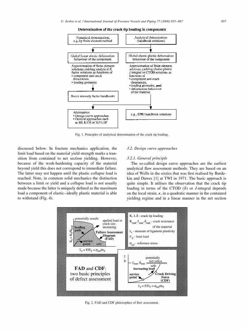
2. Failure assessment diagram or crack driving force?
The analytical ¯aw assessment methods pursue two
different philosophies, which can be designated as failure
assessment diagram (FAD) and crack driving force (CDF)
concepts (Fig. 2). In principle, the two concepts can be made
fully compatible. However, some of the methods, which
will be discussed later, prefer one of both presentations.
What is the difference? In the FAD route, a roughly
geometry-independent failure line is constructed by norma-
lising the crack tip loading by the material's fracture resis-
tance. The assessment of the component is then based on the
relative location of a geometry-dependent assessment point
with respect to this failure line. In the simplest application,
the component is regarded as safe as long as the assessment
point lies within the shaded area below the failure line. It is
regarded as potentially unsafe if it is located on the line or
outside the shaded area. An increased load or larger crack
size will move the assessment point along the loading path
towards the failure line.
In contrast to the FAD philosophy, in the CDF philosophy
the applied and material sides are strictly separated. The
determination of the crack tip loading, in the component
and its comparison with the fracture resistance of the
material are two separate steps. Like the failure line of the
FAD concept, the CDF curve can, by suitable normalisation
of the load, be made an approximately geometry-indepen-
dent function, which depends only on the deformation
behaviour of the material.
3. Analytical assessment methods
3.1. Introduction
Analytical ¯aw assessment methods have been developed
for more than 30 years. These are described in numerous
published papers but only a limited number can be discussed
within this brief survey. In addition, only the basic princi-
ples of the various methods will be reviewed. Industrial
realisations within guidelines and standards are mentioned
only in Table 1 at the end of this paper, but particularly in
this ®eld there have been rapid developments recently, as is
apparent from the other papers in this issue. Common to all
the methods discussed here is that they are not restricted to a
linear elastic deformation pattern of the material but cover
the whole range from linear elastic to elastic±plastic beha-
viour (Fig. 3).
It is important to note that the limit load of the cracked
component plays an important role in almost all the models
U. Zerbst et al. / International Journal of Pressure Vessels and Piping 77 (2000) 855±867856
Nomenclature
a Crack size
aeff Plastic zone corrected crack size (different
de®nitions for the EPRI and ETM
approaches)
E Young's modulus
E 0 E in plane stress; E=�1 2 n2� in plane strain
F Applied load (general for force, moment,
pressure, etc.)
FY Limit load
h Dimensionless function of geometry (EPRI
approach)
J J-integral
Je Linear elastic J-integral
Jmat Crack resistance in terms of critical J-integral
Jp Plastic component of the J-integral
Jssy Small scale yielding J-integral
JY J-integral at limit load
K Linear elastic stress intensity factor
Kmat Crack resistance in terms of critical K
Kr Ratio of the applied K to the crack resistance,
K/Kmat
L Characteristic length (EPRI approach)
Lr Ratio of applied load, F, to yield load, FY
Lmaxr Plastic collapse limit of Lr
N Strain hardening exponent (ETM de®nition)
n Strain hardening exponent (various de®ni-
tions)
P Applied load (EPRI approach)
Po Reference load (EPRI approach)
Rm Tensile strength
ReL Lower yield strength (materials with LuÈders
plateau)
Sr Ratio of applied load to plastic collapse load
a Fit parameter of the Ramberg±Osgood
formulation
De LuÈders strain
d CTOD
d e Linear elastic CTOD
dmat Crack resistance in terms of critical CTOD
dY CTOD at limit load
d 5 Speci®c de®nition of the CTOD (ETM
approach)
e Strain
eY Yield strain
e ref Reference strain (reference stress method)
n Poisson's ratio
s Stress
�s Flow strength (usually the average of yield
and tensile strength)
s ref Reference stress (reference stress method)
sY Yield strength
s o Normalising stress (EPRI approach)
discussed below. In fracture mechanics application, the
limit load based on the material yield strength marks a tran-
sition from contained to net section yielding. However,
because of the work-hardening capacity of the material
beyond yield this does not correspond to immediate failure.
The latter may not happen until the plastic collapse load is
reached. Note, in common solid mechanics the distinction
between a limit or yield and a collapse load is not usually
made because the latter is uniquely de®ned as the maximum
load a component of elastic±ideally plastic material is able
to withstand (Fig. 4).
3.2. Design curve approaches
3.2.1. General principle
The so-called design curve approaches are the earliest
analytical ¯aw assessment methods. They are based on an
idea of Wells in the sixties that was ®rst realised by Burde-
kin and Dawes [1] at TWI in 1971. The basic approach is
quite simple. It utilises the observation that the crack tip
loading in terms of the CTOD (d) or J-integral depends
on the local strain, e , in a quadratic manner in the contained
yielding regime and in a linear manner in the net section
U. Zerbst et al. / International Journal of Pressure Vessels and Piping 77 (2000) 855±867 857
Fig. 2. FAD and CDF philosophies of ¯aw assessment.
Fig. 1. Principles of analytical determination of the crack tip loading.
U. Zerbst et al. / International Journal of Pressure Vessels and Piping 77 (2000) 855±867858
Table 1
Overview on some methods for analytical ¯aw assessment
Basic approach Assessment routes Special features and range of application Realisation in industrial guidelines
Design curves (various
approaches mostly for CTOD)
FAD CDF No K factor solution is required where these
are based on strain, which is an advantage
for shallow crack con®gurations.
Application is usually restricted to shallow
cracks (preferably originating from
notches) and to limited ligament plasticity.
British standard BS 7910, assessment level
1, US American and Canadian documents
for welded pipelines, API 1104 and CSA
Z662, Chinese pressure vessel code CVDA-
1984; Japanese guideline WES 2805 for
¯aws in fusion welded joints.
FAD based on Dugdale model FAD Original FAD approach with the abscissa
normalised by the plastic collapse load;
should only be used for materials with a
yield to ultimate stress ratio close to unity.
BSI document PD 6493, now revised to
BS7910; `explanation document' of WES
2805.
EPRI-handbook CDF (FAD) Fully plastic solutions for the J-integral and
the CTOD derived by ®nite element
analyses. The application is restricted to a
limited number of component
con®gurations. Ramberg±Osgood
description of the stress±strain curve may
be a problem. Modi®ed versions for
strength mismatch assessment procedures
such as the American EWI and the French
ARAMIS methods.
ASME Boiler and Pressure Vessel Code,
Section XI, Appendixes G and H for
pipelines.
R6-routine FAD Based on the reference stress method of
Ainsworth, which is a generalisation of the
EPRI approach within the frame of FAD
philosophy. The R6 document includes
numerous appendices for treating weld
residual stresses and strength mismatch,
constraint effects, probabilistic sensitivity
analysis, special applications such as leak-
before-break analysis, etc.
Today the most widely applied method,
essential part of theBritish standard
BS7910, the Draft API 579 procedure of the
US American petrochemical industry, the
Swedish SAQ method, the French RSE-M
Code (2000 Addenda) for nuclear
application, and others. A partly modi®ed
version is a constituent element of the
European SINTAP procedure.
CEA-A 16 guide CDF Also based on the reference stress method.
The procedure includes guidance for leak-
before-break assessment and high
temperature creep.
Draft document for nuclear industry in
France.
ETM CDF The model is part of the comprehensive
EFAM methodology of GKSS, which
covers toughness testing and failure
assessment. In addition to the basic
procedure special options for strength
mismatch, shallow cracks at notches, and
strain-based assessment, guidance for
treating data scatter and size effects on
toughness are available.
A modi®ed version is a constituent element
of the European SINTAP procedure.
SINTAP FAD CDF Uni®ed European procedure, based on
elements of R6 and ETM as well as on
additional elements from various sources:
BS 7910, the SAQ method and others.
SINTAP includes explicitly strength
mismatch analysis, statistical treatment of
toughness data according to the VTT master
curve, compendia for stress intensity factor
and limit load solutions as well as for
residual stress pro®les, appendices for
constraint effects, reliability analysis and
special applications such as leak-before-
break analysis.
The procedure is designated for a technical
document of the CEN
yielding regime. In general terms this may be written as
d or J � eY
C1�e=eY�2 for �e=eY� , k;
C2�e=eY�1 C3 for �e=eY� . k
(�1�
with eY being the yield strain and C1,2,3 being empirical
constants. The quantity k varies within the different design
curve approaches from 0.5 to 1. In general terms, C1,2,3
depend on a range of parameters, in particular the geometry
and the loading type, for example, bending or tension. For
simplicity, these constants were derived for the centre
cracked plate loaded under tension, this being expected to
provide conservative estimates of the crack tip loading for
other con®gurations. Modern developments in design
curves tend to overcome the restriction to tension loading
and to incorporate the detailed deformation behaviour of the
material. Although solutions for deeper cracks exist, the
preferred ®eld of application is the assessment of shallow
cracks, such as those originating from notches. An advan-
tage of the design curve approaches is that they do not
require stress intensity factor solutions for the con®gura-
tions to be assessed. A dif®culty is that the strain, e , is not
clearly de®ned. Design curves can, in principle, be applied
in the frame of the FAD or CDF philosophy (Fig. 5), but are
more commonly applied in the CDF framework.
3.2.2. The TWI design curve
The most widely applied design curve approach still is
that developed by Burdekin and Dawes [1]. In CDF terms it
can be written as
d � 2peYa�e=eY�2 for �e=eY� # 0:5;
�e=eY�2 0:25 for �e=eY� . 0:5:
(�2�
In special FAD terms, the failure assessment curve becomes
FD � dmat
2peYa� �e=eY �2 for �e=eY� # 0:5;
�e=eY �2 0:25 for �e=eY� . 0:5
(�3�
for ferritic steel applications. Eq. (2) is restricted to ligament
plasticity at about the limit load of the cracked component
and to shallow cracks. The latter is due to the fact that the
crack tip loading is correlated with the applied strain, which
is usually de®ned at the outer surface of the component. The
FAD and CDF approaches of Eqs. (3) and (2) are shown in
Fig. 5a and b, respectively.
Some years later, Dawes proposed a modi®cation of Eq.
(2) for deeper cracks [2] and rewrote it in terms of stress in
order to ®t it into the FAD approach of the British PD 6493
[3] procedure. The latter modi®cation is still part of the
recently revised version of that document, the British
Standard Guide BS 7910 [4]. With some modi®cations,
the TWI design curve is also a constituent element of indus-
trial guidelines such as the US and Canadian documents for
welded pipelines, API 1104 [5] and CSA Z662 [6], and the
Chinese pressure vessel code CVDA-1984 [7].
3.2.3. The EnJ design curve
A J-integral based design curve was proposed by Turner
at Imperial College, London, in 1981 [8]. The basic equation
of the ªEnJ methodº was
J � JY
�ef =eY�2�1 1 0:5�ef =eY�2� for �ef =eY� # 1:2;
2:5 ��ef =eY �2 0:2� for �ef =eY � . 1:2
8<: �4�
with e f being the so-called ªcracked body structural strainº.
Although Turner gave expressions for e f for some basic
con®gurations, it is not clear how this is de®ned in general.
The quantity JY is the energy release rate, G, calculated
elastically, for a load equal to the limit load.
3.2.4. More recent developments
Based on extensive ®nite element analyses, a J-based
design curve approach was further developed by a group
U. Zerbst et al. / International Journal of Pressure Vessels and Piping 77 (2000) 855±867 859
Fig. 3. Application ranges of various fracture mechanics concepts. General
approaches cover all ranges within a uni®ed method.
Fig. 4. Schematics of limit and plastic collapse loads: (a) in fracture mechanics application, and (b) in common solid mechanics.
at the University of Wales, Swansea. Fitting the material's
stress±strain curve by a piece-wise power law
e=eY �s=sY for e # eY;
�s=sY�n for e . eY
(�5�
and determining the J-integral from the HRR ®eld, Lau
et al. [9] derived an expression for shallow cracks �0:05 #a=W # 0:1� and for a strain hardening exponent between
2 # n # 30 :
J � JY
�e=eY�2 for �e=eY� # 0:85;
Ce
eY
2 1:2
� ��n11�=n1JNG for �e=eY� . 1:2
8><>: �6�
with JNG and C being functions of the relative crack depth,
a/W, and the strain hardening exponent, n. J is interpolated
by a straight line between 0:85 , e=eY # 1:2: The authors
obtained a similar expression for pure bending [10], which
has recently been modi®ed for a more generalised stress±
strain curve ®t [11].
A largely independent design curve approach was devel-
oped by the Japan Welding Engineering Society (WES).
Since 1976, the WES 2805 standard and within this frame
the Japanese CTOD based design curve has been revised
several times. In the most recent version of 1997 [12] it is
given by
d �p
2eYa�e=eY�2 for �e=eY� # 1
p
8eYa�9�e=eY�2 5� for �e=eY� . 1
26643775: �7�
A special feature of the WES 2805 design curve is that the
applied strain, e , is determined from the membrane and
bending stress components across the wall and that it
depends on the strain hardening of the material if the
crack originates from a notch.
Recently Xue and Shi from the Beijing Polytechnical
University proposed a strain hardening design curve [13]
that is based on a simpli®cation of net section plastic
CTOD solutions of EPRI (see below). In a CDF format it
can be written as
d � 2peYa5n 1 3
8�n 1 1�s
sY
� �2
10:85 a ks
sY
� �n11
�8�
with s being the applied stress of the component. The
quantities a and n are the coef®cients of the Ramberg±
Osgood formulation of the stress±strain curve
e=eY � s=sY 1 a�s=sY�n �9�and k is an out-of-plane constraint factor, being
����3=2p
for
plane strain and 1 for plane stress conditions.
Finally, it has to be mentioned that the strain option of the
engineering treatment model (ETM) of the GKSS Research
Centre in Germany can also be interpreted as a design curve
approach (for more details see Ref. [14]).
3.3. Early failure assessment diagrams
3.3.1. General philosophy
The FAD for ¯aw assessment was ®rst used in the so-
called R6 approach of the former Central Electricity Gener-
ating Board (CEGB) in the UK. An overview on early
developments is given in Ref. [15]. The approach recog-
nised that, at one extreme, linear elastic fracture mechanics
was applicable and fracture occurred when the stress inten-
sity factor, K, became equal to the fracture toughness, Kmat.
At the other extreme failure occurred when the load F
reached its value, FL, at plastic collapse. The R6 approach
recognised that the use of K beyond the elastic regime
underestimated the crack tip loading and, therefore, some
plasticity correction was required, as shown in Fig. 6. In
general, this correction is a function of the material and
U. Zerbst et al. / International Journal of Pressure Vessels and Piping 77 (2000) 855±867860
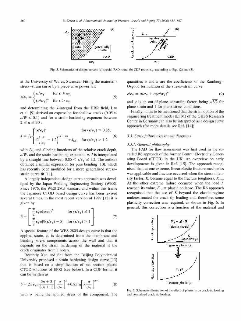
Fig. 5. Schematics of design curves: (a) special FAD route; (b) CDF route, e.g. according to Eqs. (2) and (3).
Fig. 6. Schematic illustration of the effect of plasticity on crack-tip loading
and normalised crack tip loading.
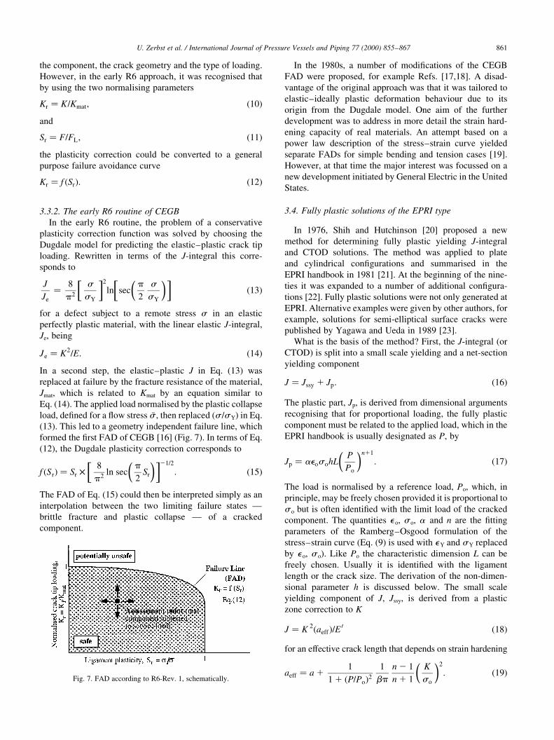
the component, the crack geometry and the type of loading.
However, in the early R6 approach, it was recognised that
by using the two normalising parameters
Kr � K=Kmat; �10�and
Sr � F=FL; �11�the plasticity correction could be converted to a general
purpose failure avoidance curve
Kr � f �Sr�: �12�
3.3.2. The early R6 routine of CEGB
In the early R6 routine, the problem of a conservative
plasticity correction function was solved by choosing the
Dugdale model for predicting the elastic±plastic crack tip
loading. Rewritten in terms of the J-integral this corre-
sponds to
J
Je
� 8
p2
s
sY
� �2
ln secp
2
s
sY
� �� ��13�
for a defect subject to a remote stress s in an elastic
perfectly plastic material, with the linear elastic J-integral,
Je, being
Je � K2=E: �14�
In a second step, the elastic±plastic J in Eq. (13) was
replaced at failure by the fracture resistance of the material,
Jmat, which is related to Kmat by an equation similar to
Eq. (14). The applied load normalised by the plastic collapse
load, de®ned for a ¯ow stress �s ; then replaced (s /sY) in Eq.
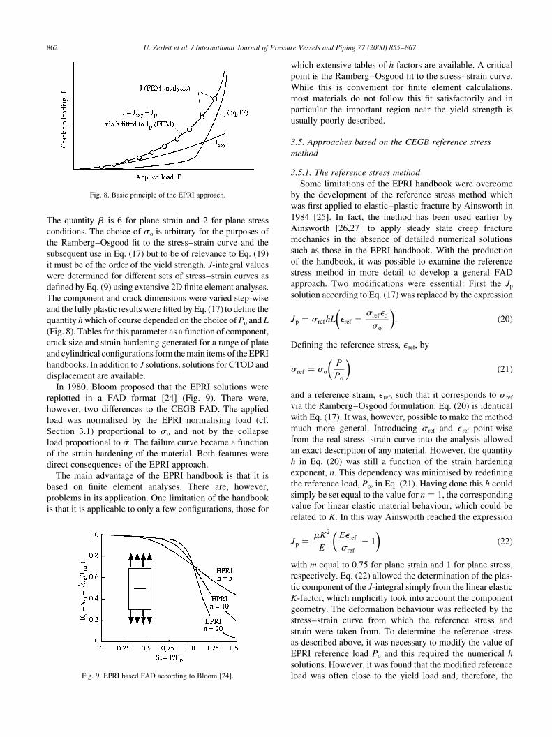
(13). This led to a geometry independent failure line, which
formed the ®rst FAD of CEGB [16] (Fig. 7). In terms of Eq.
(12), the Dugdale plasticity correction corresponds to
f �Sr� � Sr £ 8
p2ln sec
p
2Sr
� �� �21=2
: �15�
The FAD of Eq. (15) could then be interpreted simply as an
interpolation between the two limiting failure states Ð
brittle fracture and plastic collapse Ð of a cracked
component.
In the 1980s, a number of modi®cations of the CEGB
FAD were proposed, for example Refs. [17,18]. A disad-
vantage of the original approach was that it was tailored to
elastic±ideally plastic deformation behaviour due to its
origin from the Dugdale model. One aim of the further
development was to address in more detail the strain hard-
ening capacity of real materials. An attempt based on a
power law description of the stress±strain curve yielded
separate FADs for simple bending and tension cases [19].
However, at that time the major interest was focussed on a
new development initiated by General Electric in the United
States.
3.4. Fully plastic solutions of the EPRI type
In 1976, Shih and Hutchinson [20] proposed a new
method for determining fully plastic yielding J-integral
and CTOD solutions. The method was applied to plate
and cylindrical con®gurations and summarised in the
EPRI handbook in 1981 [21]. At the beginning of the nine-
ties it was expanded to a number of additional con®gura-
tions [22]. Fully plastic solutions were not only generated at
EPRI. Alternative examples were given by other authors, for
example, solutions for semi-elliptical surface cracks were
published by Yagawa and Ueda in 1989 [23].
What is the basis of the method? First, the J-integral (or
CTOD) is split into a small scale yielding and a net-section
yielding component
J � Jssy 1 Jp: �16�The plastic part, Jp, is derived from dimensional arguments
recognising that for proportional loading, the fully plastic
component must be related to the applied load, which in the
EPRI handbook is usually designated as P, by
Jp � aeosohLP
Po
� �n11
: �17�
The load is normalised by a reference load, Po, which, in
principle, may be freely chosen provided it is proportional to
s o but is often identi®ed with the limit load of the cracked
component. The quantities e o, s o, a and n are the ®tting
parameters of the Ramberg±Osgood formulation of the
stress±strain curve (Eq. (9) is used with eY and sY replaced
by e o, s o). Like Po the characteristic dimension L can be
freely chosen. Usually it is identi®ed with the ligament
length or the crack size. The derivation of the non-dimen-
sional parameter h is discussed below. The small scale
yielding component of J, Jssy, is derived from a plastic
zone correction to K
J � K 2�aeff�=E 0 �18�for an effective crack length that depends on strain hardening
aeff � a 11
1 1 �P=Po�21
bp
n 2 1
n 1 1
K
so
� �2
: �19�
U. Zerbst et al. / International Journal of Pressure Vessels and Piping 77 (2000) 855±867 861
Fig. 7. FAD according to R6-Rev. 1, schematically.
The quantity b is 6 for plane strain and 2 for plane stress
conditions. The choice of so is arbitrary for the purposes of
the Ramberg±Osgood ®t to the stress±strain curve and the
subsequent use in Eq. (17) but to be of relevance to Eq. (19)
it must be of the order of the yield strength. J-integral values
were determined for different sets of stress±strain curves as
de®ned by Eq. (9) using extensive 2D ®nite element analyses.
The component and crack dimensions were varied step-wise
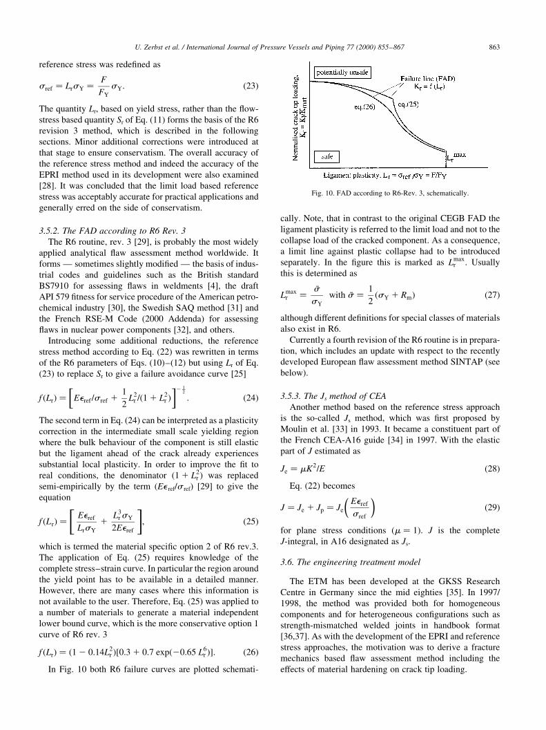
and the fully plastic results were ®tted by Eq. (17) to de®ne the
quantity h which of course depended on the choice of Po and L
(Fig. 8). Tables for this parameter as a function of component,
crack size and strain hardening generated for a range of plate
and cylindrical con®gurations form the main items of the EPRI
handbooks. In addition to J solutions, solutions for CTOD and
displacement are available.
In 1980, Bloom proposed that the EPRI solutions were
replotted in a FAD format [24] (Fig. 9). There were,
however, two differences to the CEGB FAD. The applied
load was normalised by the EPRI normalising load (cf.
Section 3.1) proportional to s o and not by the collapse
load proportional to �s : The failure curve became a function
of the strain hardening of the material. Both features were
direct consequences of the EPRI approach.
The main advantage of the EPRI handbook is that it is
based on ®nite element analyses. There are, however,
problems in its application. One limitation of the handbook
is that it is applicable to only a few con®gurations, those for
which extensive tables of h factors are available. A critical
point is the Ramberg±Osgood ®t to the stress±strain curve.
While this is convenient for ®nite element calculations,
most materials do not follow this ®t satisfactorily and in
particular the important region near the yield strength is
usually poorly described.
3.5. Approaches based on the CEGB reference stress
method
3.5.1. The reference stress method
Some limitations of the EPRI handbook were overcome
by the development of the reference stress method which
was ®rst applied to elastic±plastic fracture by Ainsworth in
1984 [25]. In fact, the method has been used earlier by
Ainsworth [26,27] to apply steady state creep fracture
mechanics in the absence of detailed numerical solutions
such as those in the EPRI handbook. With the production
of the handbook, it was possible to examine the reference
stress method in more detail to develop a general FAD
approach. Two modi®cations were essential: First the Jp
solution according to Eq. (17) was replaced by the expression
Jp � srefhL eref 2srefeo
so
� �: �20�
De®ning the reference stress, e ref, by
sref � so
P
Po
� ��21�
and a reference strain, e ref, such that it corresponds to s ref
via the Ramberg±Osgood formulation. Eq. (20) is identical
with Eq. (17). It was, however, possible to make the method
much more general. Introducing s ref and e ref point-wise
from the real stress±strain curve into the analysis allowed
an exact description of any material. However, the quantity
h in Eq. (20) was still a function of the strain hardening
exponent, n. This dependency was minimised by rede®ning
the reference load, Po, in Eq. (21). Having done this h could
simply be set equal to the value for n � 1; the corresponding
value for linear elastic material behaviour, which could be
related to K. In this way Ainsworth reached the expression
Jp � mK2
E
Eeref
sref
2 1
� ��22�
with m equal to 0.75 for plane strain and 1 for plane stress,
respectively. Eq. (22) allowed the determination of the plas-
tic component of the J-integral simply from the linear elastic
K-factor, which implicitly took into account the component
geometry. The deformation behaviour was re¯ected by the
stress±strain curve from which the reference stress and
strain were taken from. To determine the reference stress
as described above, it was necessary to modify the value of
EPRI reference load Po and this required the numerical h
solutions. However, it was found that the modi®ed reference
load was often close to the yield load and, therefore, the
U. Zerbst et al. / International Journal of Pressure Vessels and Piping 77 (2000) 855±867862
Fig. 8. Basic principle of the EPRI approach.
Fig. 9. EPRI based FAD according to Bloom [24].
reference stress was rede®ned as
sref � LrsY � F
FY
sY: �23�
The quantity Lr, based on yield stress, rather than the ¯ow-
stress based quantity Sr of Eq. (11) forms the basis of the R6
revision 3 method, which is described in the following
sections. Minor additional corrections were introduced at
that stage to ensure conservatism. The overall accuracy of
the reference stress method and indeed the accuracy of the
EPRI method used in its development were also examined
[28]. It was concluded that the limit load based reference
stress was acceptably accurate for practical applications and
generally erred on the side of conservatism.
3.5.2. The FAD according to R6 Rev. 3
The R6 routine, rev. 3 [29], is probably the most widely
applied analytical ¯aw assessment method worldwide. It
forms Ð sometimes slightly modi®ed Ð the basis of indus-
trial codes and guidelines such as the British standard
BS7910 for assessing ¯aws in weldments [4], the draft
API 579 ®tness for service procedure of the American petro-
chemical industry [30], the Swedish SAQ method [31] and
the French RSE-M Code (2000 Addenda) for assessing
¯aws in nuclear power components [32], and others.
Introducing some additional reductions, the reference
stress method according to Eq. (22) was rewritten in terms
of the R6 parameters of Eqs. (10)±(12) but using Lr of Eq.
(23) to replace Sr to give a failure avoidance curve [25]
f �Lr� � Eeref =sref 11
2L2
r =�1 1 L2r �
� �2 12
: �24�
The second term in Eq. (24) can be interpreted as a plasticity
correction in the intermediate small scale yielding region
where the bulk behaviour of the component is still elastic
but the ligament ahead of the crack already experiences
substantial local plasticity. In order to improve the ®t to
real conditions, the denominator �1 1 L2r � was replaced
semi-empirically by the term (Ee ref/s ref) [29] to give the
equation
f �Lr� � Eeref
LrsY
1L3
rsY
2Eeref
" #; �25�
which is termed the material speci®c option 2 of R6 rev.3.
The application of Eq. (25) requires knowledge of the
complete stress±strain curve. In particular the region around
the yield point has to be available in a detailed manner.
However, there are many cases where this information is
not available to the user. Therefore, Eq. (25) was applied to
a number of materials to generate a material independent
lower bound curve, which is the more conservative option 1
curve of R6 rev. 3
f �Lr� � �1 2 0:14L2r ��0:3 1 0:7 exp�20:65 L6
r ��: �26�In Fig. 10 both R6 failure curves are plotted schemati-
cally. Note, that in contrast to the original CEGB FAD the
ligament plasticity is referred to the limit load and not to the
collapse load of the cracked component. As a consequence,
a limit line against plastic collapse had to be introduced
separately. In the ®gure this is marked as Lmaxr : Usually
this is determined as
Lmaxr � �s
sY
with �s � 1
2�sY 1 Rm� �27�
although different de®nitions for special classes of materials
also exist in R6.
Currently a fourth revision of the R6 routine is in prepara-
tion, which includes an update with respect to the recently
developed European ¯aw assessment method SINTAP (see
below).
3.5.3. The Js method of CEA
Another method based on the reference stress approach
is the so-called Js method, which was ®rst proposed by
Moulin et al. [33] in 1993. It became a constituent part of
the French CEA-A16 guide [34] in 1997. With the elastic
part of J estimated as
Je � mK2=E �28�
Eq. (22) becomes
J � Je 1 Jp � Je
Eeref
sref
� ��29�
for plane stress conditions �m � 1�: J is the complete
J-integral, in A16 designated as Js.
3.6. The engineering treatment model
The ETM has been developed at the GKSS Research
Centre in Germany since the mid eighties [35]. In 1997/
1998, the method was provided both for homogeneous
components and for heterogeneous con®gurations such as
strength-mismatched welded joints in handbook format
[36,37]. As with the development of the EPRI and reference
stress approaches, the motivation was to derive a fracture
mechanics based ¯aw assessment method including the
effects of material hardening on crack tip loading.
U. Zerbst et al. / International Journal of Pressure Vessels and Piping 77 (2000) 855±867 863
Fig. 10. FAD according to R6-Rev. 3, schematically.
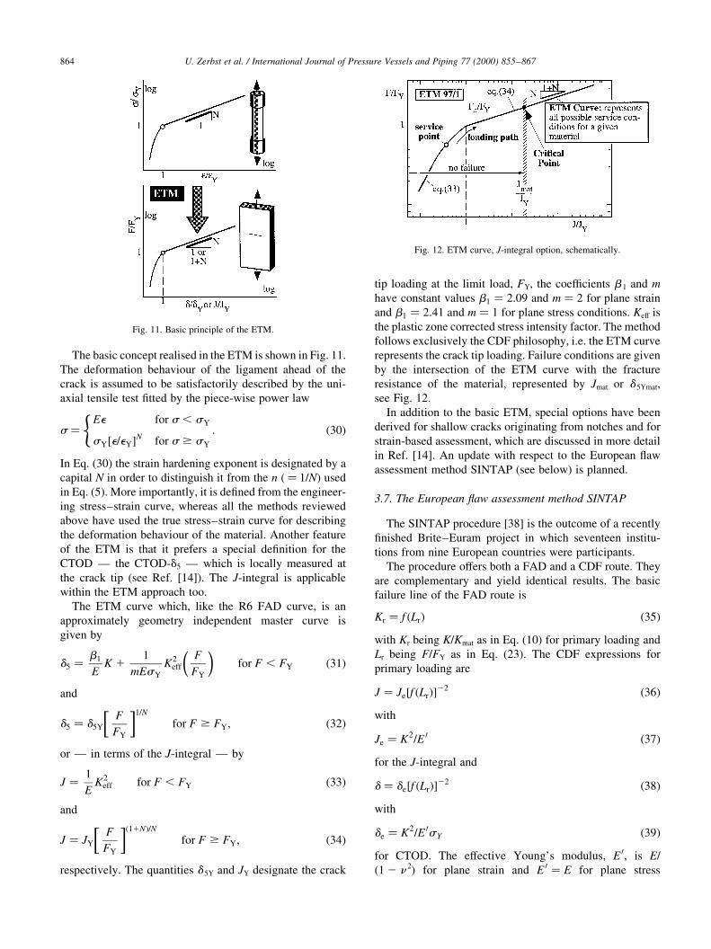
The basic concept realised in the ETM is shown in Fig. 11.
The deformation behaviour of the ligament ahead of the
crack is assumed to be satisfactorily described by the uni-
axial tensile test ®tted by the piece-wise power law
s �Ee for s , sY
sY�e=eY�N for s $ sY
(: �30�
In Eq. (30) the strain hardening exponent is designated by a
capital N in order to distinguish it from the n (� 1/N) used
in Eq. (5). More importantly, it is de®ned from the engineer-
ing stress±strain curve, whereas all the methods reviewed
above have used the true stress±strain curve for describing
the deformation behaviour of the material. Another feature
of the ETM is that it prefers a special de®nition for the
CTOD Ð the CTOD-d5 Ð which is locally measured at
the crack tip (see Ref. [14]). The J-integral is applicable
within the ETM approach too.
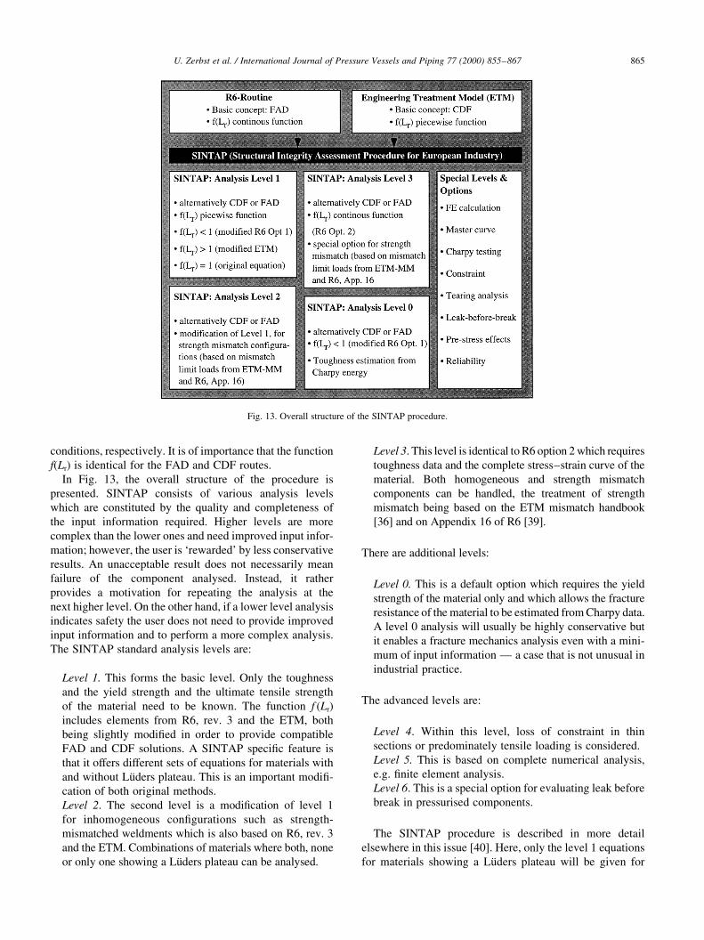
The ETM curve which, like the R6 FAD curve, is an
approximately geometry independent master curve is
given by
d5 � b1
EK 1
1
mEsY
K2eff
F
FY
� �for F , FY �31�
and
d5 � d5Y
F
FY
� �1=N
for F $ FY; �32�
or Ð in terms of the J-integral Ð by
J � 1
EK2
eff for F , FY �33�
and
J � JY
F
FY
� ��11N�=Nfor F $ FY; �34�
respectively. The quantities d 5Y and JY designate the crack
tip loading at the limit load, FY, the coef®cients b 1 and m
have constant values b1 � 2:09 and m � 2 for plane strain
and b1 � 2:41 and m � 1 for plane stress conditions. Keff is
the plastic zone corrected stress intensity factor. The method
follows exclusively the CDF philosophy, i.e. the ETM curve
represents the crack tip loading. Failure conditions are given
by the intersection of the ETM curve with the fracture
resistance of the material, represented by Jmat or d 5Ymat,
see Fig. 12.
In addition to the basic ETM, special options have been
derived for shallow cracks originating from notches and for
strain-based assessment, which are discussed in more detail
in Ref. [14]. An update with respect to the European ¯aw
assessment method SINTAP (see below) is planned.
3.7. The European ¯aw assessment method SINTAP
The SINTAP procedure [38] is the outcome of a recently
®nished Brite±Euram project in which seventeen institu-
tions from nine European countries were participants.
The procedure offers both a FAD and a CDF route. They
are complementary and yield identical results. The basic
failure line of the FAD route is
Kr � f �Lr� �35�with Kr being K/Kmat as in Eq. (10) for primary loading and
Lr being F/FY as in Eq. (23). The CDF expressions for
primary loading are
J � Je�f �Lr��22 �36�with
Je � K2=E 0 �37�
for the J-integral and
d � de�f �Lr��22 �38�with
de � K2=E 0sY �39�
for CTOD. The effective Young's modulus, E 0, is E/
(1 2 n 2) for plane strain and E 0 � E for plane stress
U. Zerbst et al. / International Journal of Pressure Vessels and Piping 77 (2000) 855±867864
Fig. 11. Basic principle of the ETM.
Fig. 12. ETM curve, J-integral option, schematically.
conditions, respectively. It is of importance that the function
f(Lr) is identical for the FAD and CDF routes.
In Fig. 13, the overall structure of the procedure is
presented. SINTAP consists of various analysis levels
which are constituted by the quality and completeness of
the input information required. Higher levels are more
complex than the lower ones and need improved input infor-
mation; however, the user is `rewarded' by less conservative
results. An unacceptable result does not necessarily mean
failure of the component analysed. Instead, it rather
provides a motivation for repeating the analysis at the
next higher level. On the other hand, if a lower level analysis
indicates safety the user does not need to provide improved
input information and to perform a more complex analysis.
The SINTAP standard analysis levels are:
Level 1. This forms the basic level. Only the toughness
and the yield strength and the ultimate tensile strength
of the material need to be known. The function f (Lr)
includes elements from R6, rev. 3 and the ETM, both
being slightly modi®ed in order to provide compatible
FAD and CDF solutions. A SINTAP speci®c feature is
that it offers different sets of equations for materials with
and without LuÈders plateau. This is an important modi®-
cation of both original methods.
Level 2. The second level is a modi®cation of level 1
for inhomogeneous con®gurations such as strength-
mismatched weldments which is also based on R6, rev. 3
and the ETM. Combinations of materials where both, none
or only one showing a LuÈders plateau can be analysed.
Level 3. This level is identical to R6 option 2 which requires
toughness data and the complete stress±strain curve of the
material. Both homogeneous and strength mismatch
components can be handled, the treatment of strength
mismatch being based on the ETM mismatch handbook
[36] and on Appendix 16 of R6 [39].
There are additional levels:
Level 0. This is a default option which requires the yield
strength of the material only and which allows the fracture
resistance of the material to be estimated from Charpy data.
A level 0 analysis will usually be highly conservative but
it enables a fracture mechanics analysis even with a mini-
mum of input information Ð a case that is not unusual in
industrial practice.
The advanced levels are:
Level 4. Within this level, loss of constraint in thin
sections or predominately tensile loading is considered.
Level 5. This is based on complete numerical analysis,
e.g. ®nite element analysis.
Level 6. This is a special option for evaluating leak before
break in pressurised components.
The SINTAP procedure is described in more detail
elsewhere in this issue [40]. Here, only the level 1 equations
for materials showing a LuÈders plateau will be given for
U. Zerbst et al. / International Journal of Pressure Vessels and Piping 77 (2000) 855±867 865
Fig. 13. Overall structure of the SINTAP procedure.
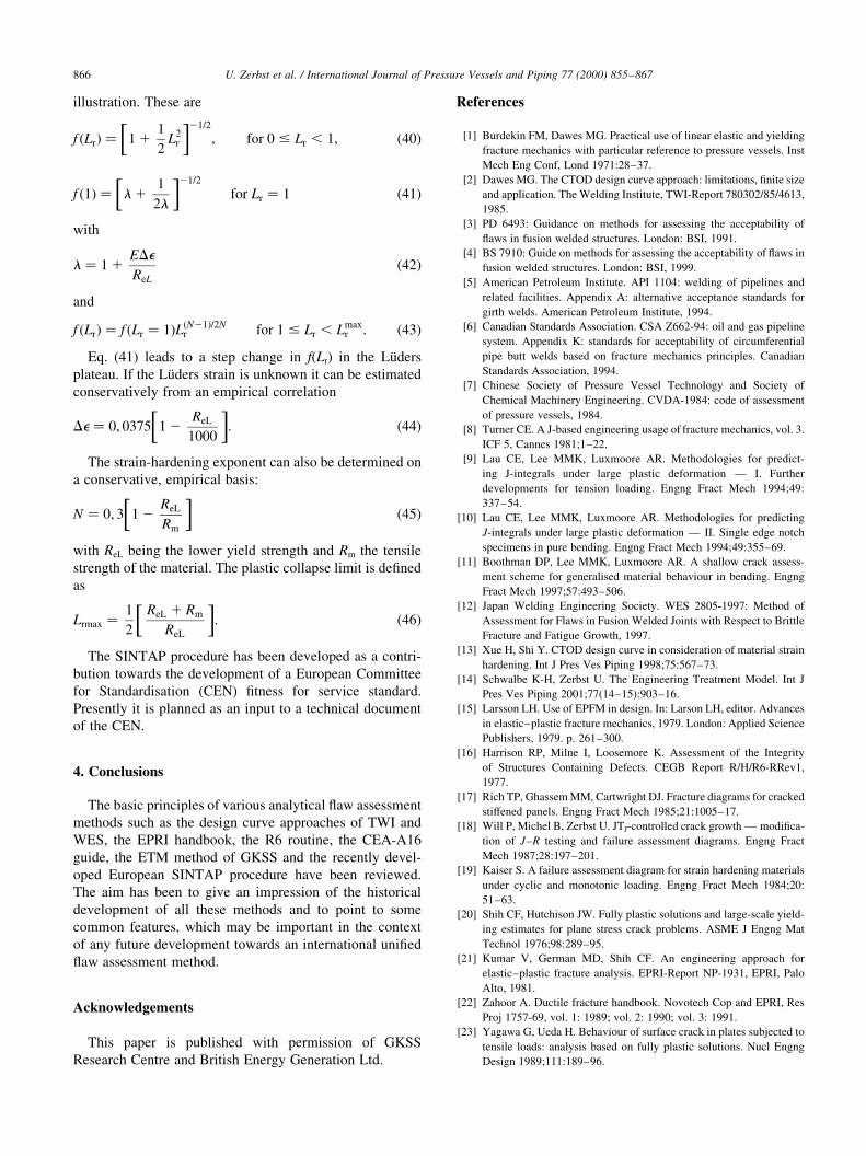
illustration. These are
f �Lr� � 1 11
2L2
r
� �21=2
; for 0 # Lr , 1; �40�
f �1� � l 11
2l
� �21=2
for Lr � 1 �41�
with
l � 1 1EDe
ReL
�42�
and
f �Lr� � f �Lr � 1�L�N21�=2Nr for 1 # Lr , Lmax
r : �43�Eq. (41) leads to a step change in f(Lr) in the LuÈders
plateau. If the LuÈders strain is unknown it can be estimated
conservatively from an empirical correlation
De � 0; 0375 1 2ReL
1000
� �: �44�
The strain-hardening exponent can also be determined on
a conservative, empirical basis:
N � 0; 3 1 2ReL
Rm
� ��45�
with ReL being the lower yield strength and Rm the tensile
strength of the material. The plastic collapse limit is de®ned
as
Lrmax � 1
2
ReL 1 Rm
ReL
� �: �46�
The SINTAP procedure has been developed as a contri-
bution towards the development of a European Committee
for Standardisation (CEN) ®tness for service standard.
Presently it is planned as an input to a technical document
of the CEN.
4. Conclusions
The basic principles of various analytical ¯aw assessment
methods such as the design curve approaches of TWI and
WES, the EPRI handbook, the R6 routine, the CEA-A16
guide, the ETM method of GKSS and the recently devel-
oped European SINTAP procedure have been reviewed.
The aim has been to give an impression of the historical
development of all these methods and to point to some
common features, which may be important in the context
of any future development towards an international uni®ed
¯aw assessment method.
Acknowledgements
This paper is published with permission of GKSS
Research Centre and British Energy Generation Ltd.
References
[1] Burdekin FM, Dawes MG. Practical use of linear elastic and yielding
fracture mechanics with particular reference to pressure vessels. Inst
Mech Eng Conf, Lond 1971:28±37.
[2] Dawes MG. The CTOD design curve approach: limitations, ®nite size
and application. The Welding Institute, TWI-Report 780302/85/4613,
1985.
[3] PD 6493: Guidance on methods for assessing the acceptability of
¯aws in fusion welded structures. London: BSI, 1991.
[4] BS 7910: Guide on methods for assessing the acceptability of ¯aws in
fusion welded structures. London: BSI, 1999.
[5] American Petroleum Institute. API 1104: welding of pipelines and
related facilities. Appendix A: alternative acceptance standards for
girth welds. American Petroleum Institute, 1994.
[6] Canadian Standards Association. CSA Z662-94: oil and gas pipeline
system. Appendix K: standards for acceptability of circumferential
pipe butt welds based on fracture mechanics principles. Canadian
Standards Association, 1994.
[7] Chinese Society of Pressure Vessel Technology and Society of
Chemical Machinery Engineering. CVDA-1984: code of assessment
of pressure vessels, 1984.
[8] Turner CE. A J-based engineering usage of fracture mechanics, vol. 3.
ICF 5, Cannes 1981;1±22.
[9] Lau CE, Lee MMK, Luxmoore AR. Methodologies for predict-
ing J-integrals under large plastic deformation Ð I. Further
developments for tension loading. Engng Fract Mech 1994;49:
337±54.
[10] Lau CE, Lee MMK, Luxmoore AR. Methodologies for predicting
J-integrals under large plastic deformation Ð II. Single edge notch
specimens in pure bending. Engng Fract Mech 1994;49:355±69.
[11] Boothman DP, Lee MMK, Luxmoore AR. A shallow crack assess-
ment scheme for generalised material behaviour in bending. Engng
Fract Mech 1997;57:493±506.
[12] Japan Welding Engineering Society. WES 2805-1997: Method of
Assessment for Flaws in Fusion Welded Joints with Respect to Brittle
Fracture and Fatigue Growth, 1997.
[13] Xue H, Shi Y. CTOD design curve in consideration of material strain
hardening. Int J Pres Ves Piping 1998;75:567±73.
[14] Schwalbe K-H, Zerbst U. The Engineering Treatment Model. Int J
Pres Ves Piping 2001;77(14±15):903±16.
[15] Larsson LH. Use of EPFM in design. In: Larson LH, editor. Advances
in elastic±plastic fracture mechanics, 1979. London: Applied Science
Publishers, 1979. p. 261±300.
[16] Harrison RP, Milne I, Loosemore K. Assessment of the Integrity
of Structures Containing Defects. CEGB Report R/H/R6-RRev1,
1977.
[17] Rich TP, Ghassem MM, Cartwright DJ. Fracture diagrams for cracked
stiffened panels. Engng Fract Mech 1985;21:1005±17.
[18] Will P, Michel B, Zerbst U. JTJ-controlled crack growth Ð modi®ca-
tion of J±R testing and failure assessment diagrams. Engng Fract
Mech 1987;28:197±201.
[19] Kaiser S. A failure assessment diagram for strain hardening materials
under cyclic and monotonic loading. Engng Fract Mech 1984;20:
51±63.
[20] Shih CF, Hutchison JW. Fully plastic solutions and large-scale yield-
ing estimates for plane stress crack problems. ASME J Engng Mat
Technol 1976;98:289±95.
[21] Kumar V, German MD, Shih CF. An engineering approach for
elastic±plastic fracture analysis. EPRI-Report NP-1931, EPRI, Palo
Alto, 1981.
[22] Zahoor A. Ductile fracture handbook. Novotech Cop and EPRI, Res
Proj 1757-69, vol. 1: 1989; vol. 2: 1990; vol. 3: 1991.
[23] Yagawa G, Ueda H. Behaviour of surface crack in plates subjected to
tensile loads: analysis based on fully plastic solutions. Nucl Engng
Design 1989;111:189±96.
U. Zerbst et al. / International Journal of Pressure Vessels and Piping 77 (2000) 855±867866
[24] Bloom JM. Prediction of ductile tearing using a proposed strain
hardening failure assessment diagram. Int J Fract 1980;6:R73±7.
[25] Ainsworth RA. The assessment of defects in structures of strain
hardening materials. Engng Fract Mech 1984;19:633±42.
[26] Milne I, Ainsworth RA, Dowling AR, Stewart AT. Assessment of the
integrity of structures containing defects. CEGB Report R/H/R6-
Revision 3. Latest ed. 1986; latest ed. British Energy, 1999.
[27] Ainsworth RA. Some observations on creep crack growth. Int J Fract
1982;20:147±59.
[28] Ainsworth RA. The initiation of creep crack growth. Int J Solids
Struct 1982;18:873±81.
[29] Miller AG, Ainsworth RA. Consistency of numerical results for
power-law hardening materials and the accuracy of the reference
stress approximation for J. Engng Fract Mech 1989;32:233±47.
[30] American Petroleum Institute. API 579. Recommended practice for
®tness-for-service, Draft, 1996.
[31] Bergman M, Brickstad B, Dahlberg L, Nilsson F, Sattari-Far I. A
procedure for safety assessment of components with cracks Ð
handbook. SA/FoU Report 91/01, AB Svensk AnlaÈggningsprovning,
Swedish Plant Inspection Ltd., 1991.
[32] RSE-M Code, 1997 ed. and 2000 Addenda: Rules for Inservice
Inspection of Nuclear Power Plant Components. AFCEN, Paris.
[33] Moulin D, Nedelec M, Clement G. Simpli®ed method to estimate J
development and application. SMIRT 1993;12(G04/4):151±6.
[34] Commissariat a l'Energie Atomique (CEA). A16: Guide for defect
assessment and leak before break analysis, Draft, 1999.
[35] Schwalbe K-H, Cornec A. The engineering treatment model (ETM)
and its practical application. Fatigue Fract Engng Mat Struct
1991;14:405±12.
[36] Schwalbe K-H, Kim Y-J, Hao S, Cornec A, KocËak M. EFAM, ETM-
MM 96: the ETM method for assessing the signi®cance of crack-like
defects in joints with mechanical heterogeneity (strength mismatch).
GKSS Report 97/E/9, 1997.
[37] Schwalbe K-H, Zerbst U, Kim Y-J, Brocks W, Cornec A, Heerens J,
Amstutz H. EFAM ETM 97: the ETM method for assessing crack-like
defects in engineering structures. GKSS Report GKSS 98/E/6, 1998.
[38] SINTAP: structural integrity assessment procedure for european
industry. Final Procedure, 1999. Brite±Euram Project No. BE95-
1426, British Steel.
[39] R6-Revision 3, Appendix 16. Allowance for strength mismatch
effects, British Energy, 1997.
[40] Ainsworth RA, Bannister AC, Zerbst U. An overview of the European
¯aw assessment procedure SINTAP and its validation. Int J Pres Ves
Piping 2001;77(14±15):869±76.
U. Zerbst et al. / International Journal of Pressure Vessels and Piping 77 (2000) 855±867 867
Recommended