EXTRAPOLATION TECHNIQUES FOR VERY LOW CYCLE
FATIGUE BEHAVIOR OF A NI-BASE SUPERALLOY
by
BRIAN R. DAUBENSPECK
A thesis submitted in partial fulfillment of the requirements
for the Honors in the Major program
in the Department of Mechanical, Materials, and Aerospace Engineering
in the College of Engineering and Computer Science
and in The Burnett Honors College
at the University of Central Florida
Orlando, Florida
Spring Term 2010
Thesis Chair: Dr. Ali P. Gordon
ABSTRACT
This thesis describes innovative methods used to predict high-stress amplitude, low cycle
fatigue (LCF) behavior of a material commonly used in gas turbine blade design with the
absence of such data. A combination of extrapolation and estimation techniques from
both prior and current studies has been explored with the goal of developing a method to
accurately characterize such high-temperature fatigue of IN738LC, a dual-phase Ni-base
superalloy. A method capable of predicting high-stress (or strain) amplitude fatigue from
incessantly available low-stress amplitude, high cycle fatigue (HCF) would lower the
costs of inspection, repair, and replacement on certain turbine components. Three sets of
experimental data at different temperatures are used to evaluate and examine the validity
of extrapolation methods such as anchor points and hysteresis energy trends. Stemming
from extrapolation techniques developed earlier by Coffin, Manson, and Basquin, the
techniques exercised in this study purely implement tensile test and HCF data with
limited plastic strain during the estimation processes. A standard practice in engineering
design necessitates mechanical testing closely resembling planned service conditions; for
design against fatigue failure, HCF and tensile data are the experiments of choice. High
stress amplitude data points approaching the ultimate strength of the material were added
to the pre-existing HCF base data to achieve a full-range data set that could be used to
test the legitimacy of the different prediction methods. While some methods proved to be
useful for bounding estimates, others provided for superior estimation.

iii
DEDICATION
For Sam and Dianne Daubenspeck, my parents, who gave me everything.

iv
ACKOWLEDGEMENTS
I would like to convey my genuine thanks and appreciation to my thesis chair and
research advisor, Dr. Ali Gordon, for his guidance and unwavering encouragement.
Thanks to my committee members who interminably supported me throughout the
development of my thesis.
The fatigue tests presented in this thesis were prepared by David Radonovich and
conducted at Siemens test lab in Casselberry, Florida; their efforts and technical support
are highly valued. The individual assistance of Dr. Sachin Shinde of Siemens Power
Generation is also highly appreciated.
v
TABLE OF CONTENTS
LIST OF FIGURES .............................................................................................. vii
LIST OF TABLES .................................................................................................ix
NOMENCLATURE ............................................................................................... x
1. Introduction ....................................................................................................... 1
1.1. Foreword .............................................................................................. 1
1.2. Test Material ........................................................................................ 3
2. Background ...................................................................................................... 8
2.1. Strain-Life Approach ............................................................................ 8
2.2. Strain Energy Density ........................................................................ 13
2.3. Anchor Points ..................................................................................... 16
2.4. Literature Review ............................................................................... 18
2.4.1. Ni-base Superalloy Studies ................................................................ 18
2.4.2. Existing Approximation Techniques ................................................... 21
2.5. Hypotheses ........................................................................................ 25
3. Approach ........................................................................................................ 28
3.1. Experimentation ................................................................................. 28
3.2. Experimental Results ......................................................................... 31
3.3. Model 1 – Modified Anchor Point ....................................................... 34
3.4. Model 2 – Weighting of Higher Plasticity Base Data .......................... 35
3.5. Model 3 – Original Basquin’s Equation Perpetuation ......................... 36
3.6. Model 4 – Plastic Hysteresis Energy Density Trends ......................... 36
4. Model Results ................................................................................................. 38
4.1. Data Representation .......................................................................... 38
4.2. Model Comparison ............................................................................. 39
5. Discussion ...................................................................................................... 55
5.1. Modified Anchor Point Based Models ................................................ 55
5.2. Weighting of Increased Plasticity Based Models ................................ 56
5.3. Plastic Hysteresis Energy Model ........................................................ 57
vi
5.4. Additional Remarks ............................................................................ 60
6. Conclusions .................................................................................................... 63
7. Future Work .................................................................................................... 65
APPENDIX A: EXPERIMENTAL TEST RESULTS ............................................. 66
APPENDIX B: ITERATIVE DEVELOPMENT OF STRAIN-LIFE FATIGUE
CONSTANTS ..................................................................................................... 76
REFERENCES ................................................................................................... 83
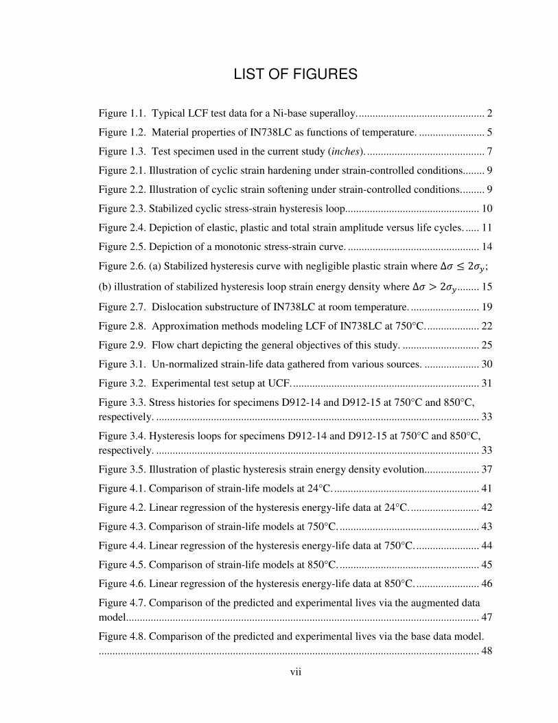
vii
LIST OF FIGURES
Figure 1.1. Typical LCF test data for a Ni-base superalloy. .............................................. 2
Figure 1.2. Material properties of IN738LC as functions of temperature. ........................ 5
Figure 1.3. Test specimen used in the current study (inches). ........................................... 7
Figure 2.1. Illustration of cyclic strain hardening under strain-controlled conditions. ....... 9
Figure 2.2. Illustration of cyclic strain softening under strain-controlled conditions. ........ 9
Figure 2.3. Stabilized cyclic stress-strain hysteresis loop................................................. 10
Figure 2.4. Depiction of elastic, plastic and total strain amplitude versus life cycles. ..... 11
Figure 2.5. Depiction of a monotonic stress-strain curve. ................................................ 14
Figure 2.6. (a) Stabilized hysteresis curve with negligible plastic strain where ∆� � 2��;
(b) illustration of stabilized hysteresis loop strain energy density where ∆� � 2��........ 15
Figure 2.7. Dislocation substructure of IN738LC at room temperature. ......................... 19
Figure 2.8. Approximation methods modeling LCF of IN738LC at 750°C. ................... 22
Figure 2.9. Flow chart depicting the general objectives of this study. ............................ 25
Figure 3.1. Un-normalized strain-life data gathered from various sources. .................... 30
Figure 3.2. Experimental test setup at UCF. .................................................................... 31
Figure 3.3. Stress histories for specimens D912-14 and D912-15 at 750°C and 850°C,
respectively. ...................................................................................................................... 33
Figure 3.4. Hysteresis loops for specimens D912-14 and D912-15 at 750°C and 850°C,
respectively. ...................................................................................................................... 33
Figure 3.5. Illustration of plastic hysteresis strain energy density evolution. ................... 37
Figure 4.1. Comparison of strain-life models at 24°C. ..................................................... 41
Figure 4.2. Linear regression of the hysteresis energy-life data at 24°C. ......................... 42
Figure 4.3. Comparison of strain-life models at 750°C. ................................................... 43
Figure 4.4. Linear regression of the hysteresis energy-life data at 750°C. ....................... 44
Figure 4.5. Comparison of strain-life models at 850°C. ................................................... 45
Figure 4.6. Linear regression of the hysteresis energy-life data at 850°C. ....................... 46
Figure 4.7. Comparison of the predicted and experimental lives via the augmented data
model................................................................................................................................. 47
Figure 4.8. Comparison of the predicted and experimental lives via the base data model.
........................................................................................................................................... 48
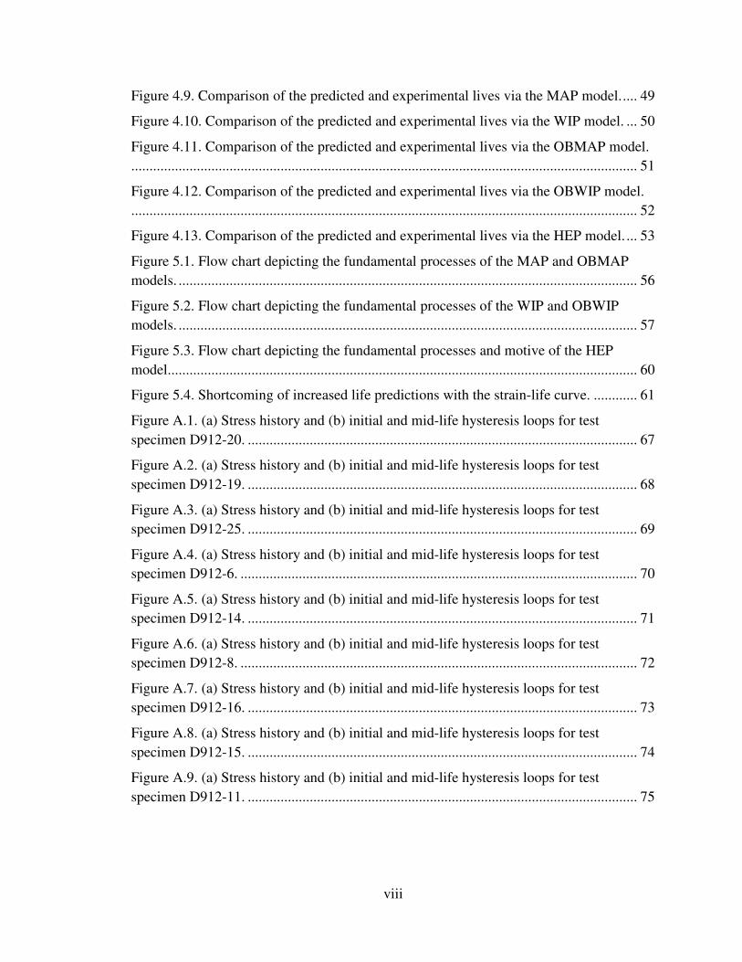
viii
Figure 4.9. Comparison of the predicted and experimental lives via the MAP model. .... 49
Figure 4.10. Comparison of the predicted and experimental lives via the WIP model. ... 50
Figure 4.11. Comparison of the predicted and experimental lives via the OBMAP model.
........................................................................................................................................... 51
Figure 4.12. Comparison of the predicted and experimental lives via the OBWIP model.
........................................................................................................................................... 52
Figure 4.13. Comparison of the predicted and experimental lives via the HEP model. ... 53
Figure 5.1. Flow chart depicting the fundamental processes of the MAP and OBMAP
models. .............................................................................................................................. 56
Figure 5.2. Flow chart depicting the fundamental processes of the WIP and OBWIP
models. .............................................................................................................................. 57
Figure 5.3. Flow chart depicting the fundamental processes and motive of the HEP
model................................................................................................................................. 60
Figure 5.4. Shortcoming of increased life predictions with the strain-life curve. ............ 61
Figure A.1. (a) Stress history and (b) initial and mid-life hysteresis loops for test
specimen D912-20. ........................................................................................................... 67
Figure A.2. (a) Stress history and (b) initial and mid-life hysteresis loops for test
specimen D912-19. ........................................................................................................... 68
Figure A.3. (a) Stress history and (b) initial and mid-life hysteresis loops for test
specimen D912-25. ........................................................................................................... 69
Figure A.4. (a) Stress history and (b) initial and mid-life hysteresis loops for test
specimen D912-6. ............................................................................................................. 70
Figure A.5. (a) Stress history and (b) initial and mid-life hysteresis loops for test
specimen D912-14. ........................................................................................................... 71
Figure A.6. (a) Stress history and (b) initial and mid-life hysteresis loops for test
specimen D912-8. ............................................................................................................. 72
Figure A.7. (a) Stress history and (b) initial and mid-life hysteresis loops for test
specimen D912-16. ........................................................................................................... 73
Figure A.8. (a) Stress history and (b) initial and mid-life hysteresis loops for test
specimen D912-15. ........................................................................................................... 74
Figure A.9. (a) Stress history and (b) initial and mid-life hysteresis loops for test
specimen D912-11. ........................................................................................................... 75
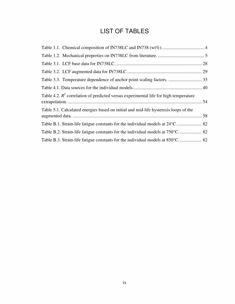
ix
LIST OF TABLES
Table 1.1. Chemical composition of IN738LC and IN738 (wt%). .................................... 4
Table 1.2. Mechanical properties on IN738LC from literature. ........................................ 5
Table 3.1. LCF base data for IN738LC. .......................................................................... 28
Table 3.2. LCF augmented data for IN738LC. ................................................................ 29
Table 3.3. Temperature dependence of anchor point scaling factors. ............................. 35
Table 4.1. Data sources for the individual models............................................................ 40
Table 4.2. R2 correlation of predicted versus experimental life for high temperature
extrapolation. .................................................................................................................... 54
Table 5.1. Calculated energies based on initial and mid-life hysteresis loops of the
augmented data. ................................................................................................................ 58
Table B.1. Strain-life fatigue constants for the individual models at 24°C. ..................... 82
Table B.2. Strain-life fatigue constants for the individual models at 750°C. ................... 82
Table B.3. Strain-life fatigue constants for the individual models at 850°C. ................... 82
x
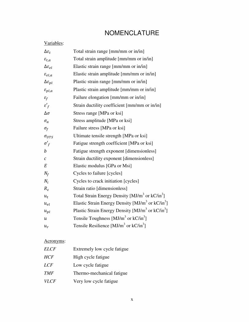
NOMENCLATURE
Variables:
∆�� Total strain range [mm/mm or in/in]
��, Total strain amplitude [mm/mm or in/in]
∆��� Elastic strain range [mm/mm or in/in]
���, Elastic strain amplitude [mm/mm or in/in]
∆� � Plastic strain range [mm/mm or in/in]
� �, Plastic strain amplitude [mm/mm or in/in]
�� Failure elongation [mm/mm or in/in]
��� Strain ductility coefficient [mm/mm or in/in]
∆� Stress range [MPa or ksi]
� Stress amplitude [MPa or ksi]
�� Failure stress [MPa or ksi]
���� Ultimate tensile strength [MPa or ksi]
��� Fatigue strength coefficient [MPa or ksi]
� Fatigue strength exponent [dimensionless]
� Strain ductility exponent [dimensionless]
� Elastic modulus [GPa or Msi]
�� Cycles to failure [cycles]
�� Cycles to crack initiation [cycles]
�� Strain ratio [dimensionless]
�� Total Strain Energy Density [MJ/m3 or kC/in
3]
��� Elastic Strain Energy Density [MJ/m3 or kC/in
3]
� � Plastic Strain Energy Density [MJ/m3 or kC/in
3]
� Tensile Toughness [MJ/m3 or kC/in
3]
�� Tensile Resilience [MJ/m3 or kC/in
3]
Acronyms:
ELCF Extremely low cycle fatigue
HCF High cycle fatigue
LCF Low cycle fatigue
TMF Thermo-mechanical fatigue
VLCF Very low cycle fatigue
1
1. Introduction
1.1. Foreword
Accurate fatigue data are essential for the design of contemporary gas turbines
under not only working loads, but accidental and manufacturing loads also having a
cyclic nature. Components in these devices are subjected to combinations of high
temperature and mechanical cycling. A broad range of fatigue data increases this
accuracy by providing insight to cyclic plastic strain. In most cases, there is a sufficient
amount of both HCF and relatively low-stress LCF data to ensure reliability within the
common loading cycles. Characteristically, low cycle fatigue data are obtained via
additional mechanical testing, which can be tedious and expensive (Radonovich and
Gordon, 2008). Acquiring the LCF data from a pre-existing HCF data set would be of
utmost efficiency. A strain-life based fatigue curve consists of two linear sets of data to
which a curve is fit: elastic strain data, which are always plentiful, and plastic strain data.
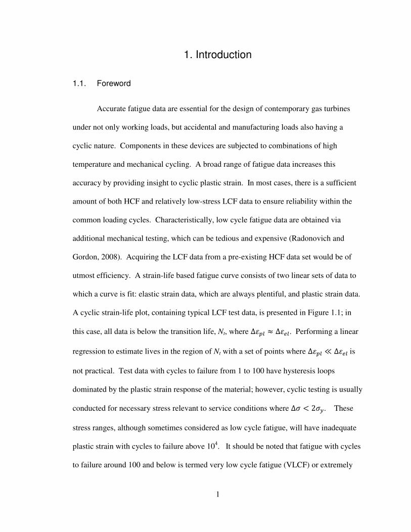
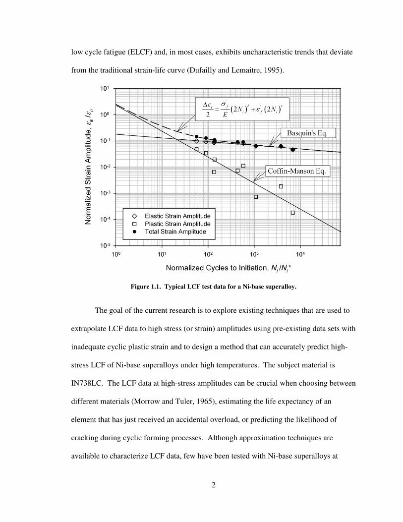
A cyclic strain-life plot, containing typical LCF test data, is presented in Figure 1.1; in
this case, all data is below the transition life, Nt, where ∆� � � ∆���. Performing a linear
regression to estimate lives in the region of Nt with a set of points where ∆� � � ∆��� is
not practical. Test data with cycles to failure from 1 to 100 have hysteresis loops
dominated by the plastic strain response of the material; however, cyclic testing is usually
conducted for necessary stress relevant to service conditions where ∆� � 2��. These
stress ranges, although sometimes considered as low cycle fatigue, will have inadequate
plastic strain with cycles to failure above 104. It should be noted that fatigue with cycles
to failure around 100 and below is termed very low cycle fatigue (VLCF) or extremely
2
low cycle fatigue (ELCF) and, in most cases, exhibits uncharacteristic trends that deviate
from the traditional strain-life curve (Dufailly and Lemaitre, 1995).
Figure 1.1. Typical LCF test data for a Ni-base superalloy.
The goal of the current research is to explore existing techniques that are used to
extrapolate LCF data to high stress (or strain) amplitudes using pre-existing data sets with
inadequate cyclic plastic strain and to design a method that can accurately predict high-
stress LCF of Ni-base superalloys under high temperatures. The subject material is
IN738LC. The LCF data at high-stress amplitudes can be crucial when choosing between
different materials (Morrow and Tuler, 1965), estimating the life expectancy of an
element that has just received an accidental overload, or predicting the likelihood of
cracking during cyclic forming processes. Although approximation techniques are
available to characterize LCF data, few have been tested with Ni-base superalloys at
3
elevated temperatures. Eminent methods of approximation such as Manson’s Universal
Slopes (Manson, 1965; Manson, 1968), Manson’s Four Point (Manson, 1965), and the
Modified Four Point by Ong (1993), originally designed for room temperature steel
alloys, have little correlation with the high-temperature LCF data of IN738LC. These
approximation methods are generally calculated based on historical observations from
phenomenological behavior and/or functions of tensile test properties (Radonovich and
Gordon, 2008). Less broadly-used methods that exist for LCF predictions of Ni-base
superalloys are only useful for estimating boundaries of fatigue life and may only be
effective for material selection purposes. Considering that there are several uses of Ni-
base superalloys, in this case gas turbine components, the development of a technique to
either extrapolate to or estimate high-stress amplitude fatigue within these alloys for
wide-ranging temperatures would be an extraordinary contribution to the gas turbine
industry.
1.2. Test Material
Gas turbine engines are designed to operate at a maximum temperature between
1100°C and 1300°C, but due to coatings and cooling techniques most experimental test
data are needed in the range of 750°C and 950°C (Albeirutty et al., 2004). In the hot gas
path region, Ni-base superalloys are often employed due to their strength against creep
and fatigue mechanisms of damage. For this study, Ni-base superalloy IN738LC
(Inconel 738 Low Carbon) is used. In particular, LCF data for this material is widely
available through open literature (Marchionni et al., 1982; Jianting and Ranucci, 1983;
Jianting et al., 1984; Day and Thomas, 1985; Fischmeister et al., 1986; Persson et al.,
1986; Matsuda et al., 1986; Onodera and Ro, 1986). Conversely, limited VLCF data is
4
available, even though an extensive review of literature was conducted. The superior
properties of IN738LC are attributed to an FCC (face-centered-cubic) matrix that is
hardened by apt solutes and fine precipitates (Balikci, 1998). The precipitates, termed �, strengthen the material by slowing down dislocations; this phase makes up 48% of the
total volume. Along with the matrix and � phase, this multiphase alloy consists of
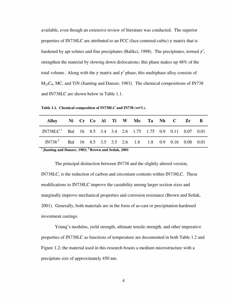
M23C6, MC, and TiN (Jianting and Danzer, 1983). The chemical compositions of IN738
and IN738LC are shown below in Table 1.1.
Table 1.1. Chemical composition of IN738LC and IN738 (wt%).
Alloy Ni Cr Co Al Ti W Mo Ta Nb C Zr B
IN738LC 1
Bal 16 8.5 3.4 3.4 2.6 1.75 1.75 0.9 0.11 0.07 0.01
IN738 2
Bal 16 8.5 3.5 3.5 2.6 1.8 1.8 0.9 0.16 0.08 0.01
1 Jianting and Danzer, 1983;
2 Brown and Setlak, 2001
The principal distinction between IN738 and the slightly altered version,
IN738LC, is the reduction of carbon and zirconium contents within IN738LC. These
modifications to IN738LC improve the castability among larger section sizes and
marginally improve mechanical properties and corrosion resistance (Brown and Setlak,
2001). Generally, both materials are in the form of as-cast or precipitation-hardened
investment castings.
Young’s modulus, yield strength, ultimate tensile strength, and other imperative
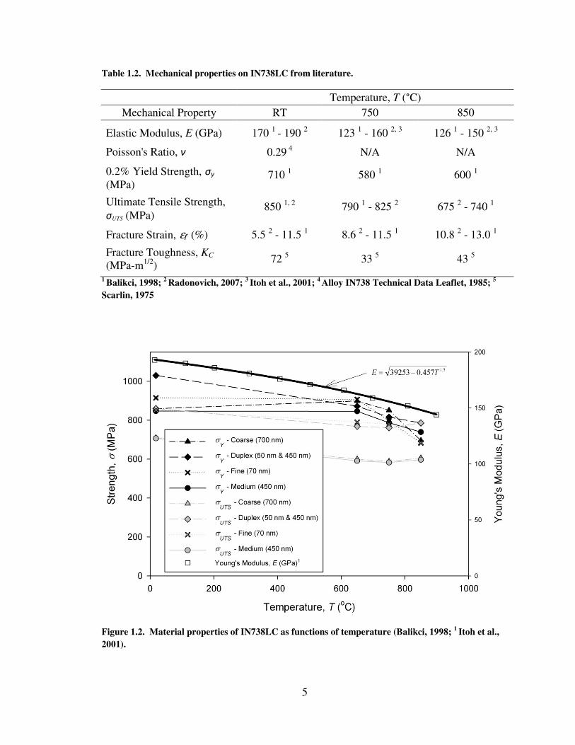
properties of IN738LC as functions of temperature are documented in both Table 1.2 and
Figure 1.2; the material used in this research boasts a medium microstructure with a
precipitate size of approximately 450 nm.
5
Table 1.2. Mechanical properties on IN738LC from literature.
Temperature, T (°C)
Mechanical Property RT 750 850
Elastic Modulus, E (GPa) 170 1
- 190 2 123
1 - 160
2, 3 126
1 - 150
2, 3
Poisson's Ratio, ν 0.29 4
N/A N/A
0.2% Yield Strength, σy
(MPa) 710
1 580
1 600
1
Ultimate Tensile Strength,
σUTS (MPa) 850
1, 2 790
1 - 825
2 675
2 - 740
1
Fracture Strain, εf (%) 5.5 2 - 11.5
1 8.6
2 - 11.5
1 10.8
2 - 13.0
1
Fracture Toughness, KC
(MPa-m1/2
) 72
5 33
5 43
5
1 Balikci, 1998;
2 Radonovich, 2007;
3 Itoh et al., 2001;
4 Alloy IN738 Technical Data Leaflet, 1985;
5
Scarlin, 1975
Figure 1.2. Material properties of IN738LC as functions of temperature (Balikci, 1998; 1 Itoh et al.,
2001).
6
Although the overall strength of the material decreases with increasing temperature, the
mechanical properties of IN738LC remain superior in high-temperature conditions. The
increase in yield strength for the medium, coarse, and duplex microstructures with
temperatures following 750°C is also noteworthy. Many Ni-based superalloys have a
similar chemical makeup and are used in parallel with IN738LC in turbine engine design
(Petrenec et al., 2007).
The mechanical test data used in this research includes tensile results and fully-
reversed cyclic tests at 24°C, 750°C, and 850°C; these temperatures are commonly
realized in turbine blades. Fiscal incentives exist to fully utilize less expensive cast
superalloys, such as IN738LC, as opposed to superior directionally-solidified (DS) or
single crystal (SC) alloys. Both DS and SC Ni-base superalloys provide for advanced
fatigue and creep properties and are often used in turbine blade construction, but are not
always cost effective with a high ratio of price to performance (Hou et al., 2009).
The typical processing conditions for specimens machined from cast slabs of
IN738LC can vary. The IN738LC material is generally hot isostatically pressed (HIP’d)
for between one and four hours under 75-125 MPa at 1100-1300°C and then cooled
slowly at a controlled rate while appropriately depressurizing (Balikci, 1998;
Radonovich, 2007). After maintaining the slab at around 1100°C for several more hours,
the material is gas quenched to room temperature in less than five minutes. Precipitation
hardening is then generally achieved via heating, cooling, and thermal shocking
techniques. Rod stock is incised from the cast slabs via electrical discharge machining
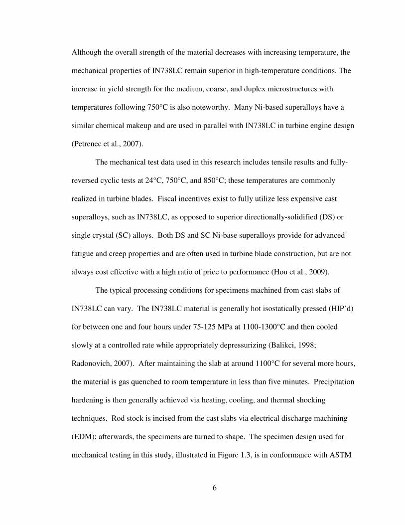
(EDM); afterwards, the specimens are turned to shape. The specimen design used for
mechanical testing in this study, illustrated in Figure 1.3, is in conformance with ASTM
7
standard E606-04 (2004). A 0.75 inch gage length is employed with a 0.25 inch diameter
and an axially polished 0.2 µm surface finish.
Figure 1.3. Test specimen used in the current study (inches).
The remainder of this thesis highlights the merits and limitations of published
work focusing on fatigue characterization of Ni-base superalloys, proposes solutions for
the candidate material, and illustrates attributes and contributions acquired thereof.
Following an extensive review of fundamental methods of fatigue evaluation, Chapter 2
continues with a literature review that demonstrates approaches exercised thus far to
characterize the mechanical properties of a variety of materials, primarily Ni-base
superalloys. A novel set of hypotheses is then established based on previous work and
data availability. Subsequently, in the 3rd
chapter, methods of ascertaining the validity of
these suppositions are constructed. After an examination of the results in Chapter 4, a
thorough discussion, within the 5th
chapter, is offered detailing the accomplishments of
each technique. Ultimately, conclusions focusing on the successes and failures of the
study are presented in Chapter 6 followed by modifications that could be employed to
augment future research in the 7th
and final chapter.
8
2. Background
2.1. Strain-Life Approach
There exist various methods capable of evaluating the range of fatigue regimens:
stress-life (HCF), strain-life (LCF), and fracture mechanics (HCF and LCF). The stress-
life approach was the original method proposed to measure fatigue within metals and
remains a standard for design applications where cycles to failure are well above 104 and
realized stress remains predominantly elastic below the yield strength of the material.
Considering the plastic behavior and the required physical insight into damage
mechanisms at short lives (102-10
4), the stress-life technique is incapable of delineating
LCF. The strain-life curve conversely, was designed to manage such short life
appliances.
The merit of this strain-life approach is the direct inclusion of plastic strain into
curve development. When the stresses being cyclically induced are above the yield
strength of a component, the material response strongly depends on its strain hardening
properties. The consequence is stress-saturation, and in such cases force-controlled
cycling leads to much scatter in life. Completely-reversed strain-controlled cyclic fatigue
tests are carried out to construct strain-life curves. Data from the experiments are post-
processed to develop stress history plots and stress-strain hysteresis loops. It should be
noted that completed-reversed tests are presented in this study where the mean stress, �!,
is zero; however, this form of testing is not a requirement for strain-life analyses.
Both stress history and hysteresis plots can be used to illustrate either strain
hardening or softening. Strain hardening often occurs when dislocation density increases
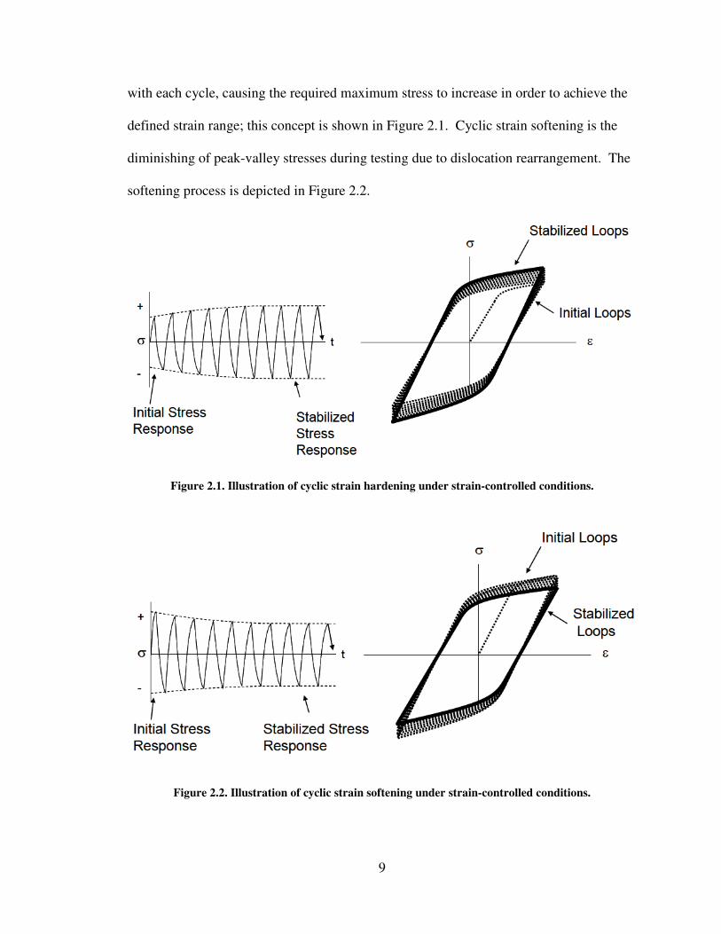
9
with each cycle, causing the required maximum stress to increase in order to achieve the
defined strain range; this concept is shown in Figure 2.1. Cyclic strain softening is the
diminishing of peak-valley stresses during testing due to dislocation rearrangement. The
softening process is depicted in Figure 2.2.
Figure 2.1. Illustration of cyclic strain hardening under strain-controlled conditions.
Figure 2.2. Illustration of cyclic strain softening under strain-controlled conditions.
10
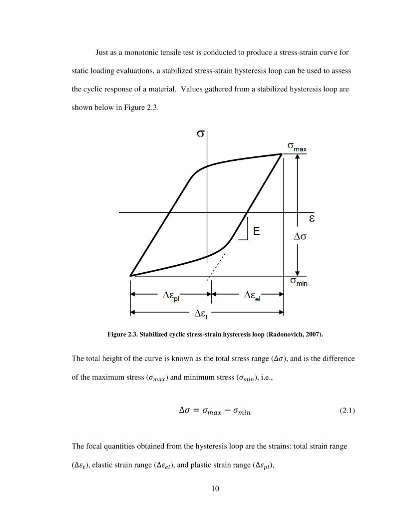
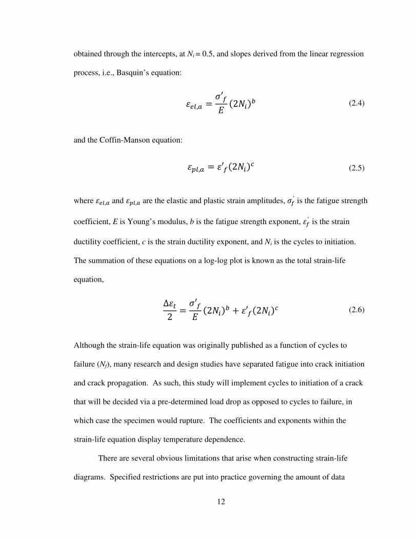
Just as a monotonic tensile test is conducted to produce a stress-strain curve for
static loading evaluations, a stabilized stress-strain hysteresis loop can be used to assess
the cyclic response of a material. Values gathered from a stabilized hysteresis loop are
shown below in Figure 2.3.
Figure 2.3. Stabilized cyclic stress-strain hysteresis loop (Radonovich, 2007).
The total height of the curve is known as the total stress range (∆�), and is the difference
of the maximum stress (�!") and minimum stress (�!�#), i.e.,
∆� $ �!" % �!�# (2.1)
The focal quantities obtained from the hysteresis loop are the strains: total strain range
(∆��), elastic strain range (∆���), and plastic strain range (∆� �),
11
∆�� $ ∆��� & ∆� � (2.2)
These strains are halved into strain amplitudes, �, and then used as data on the strain-life
diagram, i.e.,
� $ ∆�2 (2.3)
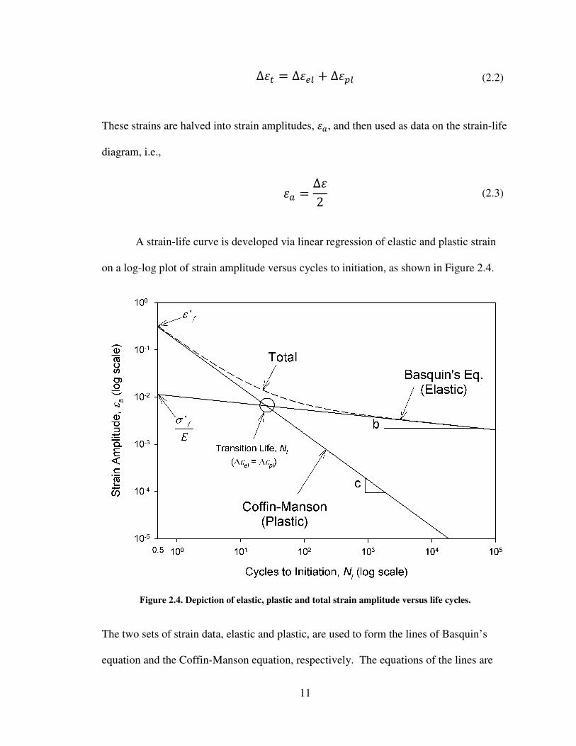
A strain-life curve is developed via linear regression of elastic and plastic strain
on a log-log plot of strain amplitude versus cycles to initiation, as shown in Figure 2.4.
Figure 2.4. Depiction of elastic, plastic and total strain amplitude versus life cycles.
The two sets of strain data, elastic and plastic, are used to form the lines of Basquin’s
equation and the Coffin-Manson equation, respectively. The equations of the lines are
12
obtained through the intercepts, at Ni = 0.5, and slopes derived from the linear regression
process, i.e., Basquin’s equation:
���, $ ���� '2��() (2.4)
and the Coffin-Manson equation:
� �, $ ���'2��(* (2.5)
where ���, and � �, are the elastic and plastic strain amplitudes, ��′ is the fatigue strength
coefficient, E is Young’s modulus, b is the fatigue strength exponent, ��′ is the strain
ductility coefficient, c is the strain ductility exponent, and Ni is the cycles to initiation.
The summation of these equations on a log-log plot is known as the total strain-life
equation,
∆��2 $ ���
� '2��() & ���'2��(* (2.6)
Although the strain-life equation was originally published as a function of cycles to
failure (Nf), many research and design studies have separated fatigue into crack initiation
and crack propagation. As such, this study will implement cycles to initiation of a crack
that will be decided via a pre-determined load drop as opposed to cycles to failure, in
which case the specimen would rupture. The coefficients and exponents within the
strain-life equation display temperature dependence.
There are several obvious limitations that arise when constructing strain-life
diagrams. Specified restrictions are put into practice governing the amount of data
13
needed to accurately define fatigue constants. The ASTM standard E739-91 (2004)
suggests that there are both preliminary and design quality levels attainable when
developing a strain-life plot. For a preliminary quality level, six to twelve tests are
recommended; twice these amounts are needed for design. The more evident restraints
are observed when using linear regression to define the Coffin-Manson equation.
Plastically inferior data, as achieved when generated cyclic stress levels are barely above
the yield strength, can significantly skew the regression process. The biased nature of
this HCF data makes the extrapolation processes of plastic data especially problematic.
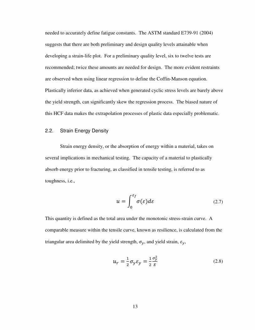
2.2. Strain Energy Density
Strain energy density, or the absorption of energy within a material, takes on
several implications in mechanical testing. The capacity of a material to plastically
absorb energy prior to fracturing, as classified in tensile testing, is referred to as
toughness, i.e.,
� $ + �'�(,��-
. (2.7)
This quantity is defined as the total area under the monotonic stress-strain curve. A
comparable measure within the tensile curve, known as resilience, is calculated from the
triangular area delimited by the yield strength, ��, and yield strain, ��,
�� $ /0���� $ /
01234 (2.8)
14
Resilience is the ability of a material to recoverably absorb elastic energy during
deformation. An improved comprehension of both the toughness and resilience can be
taken from the stress-strain tensile curve represented in Figure 2.5.
Figure 2.5. Depiction of a monotonic stress-strain curve.
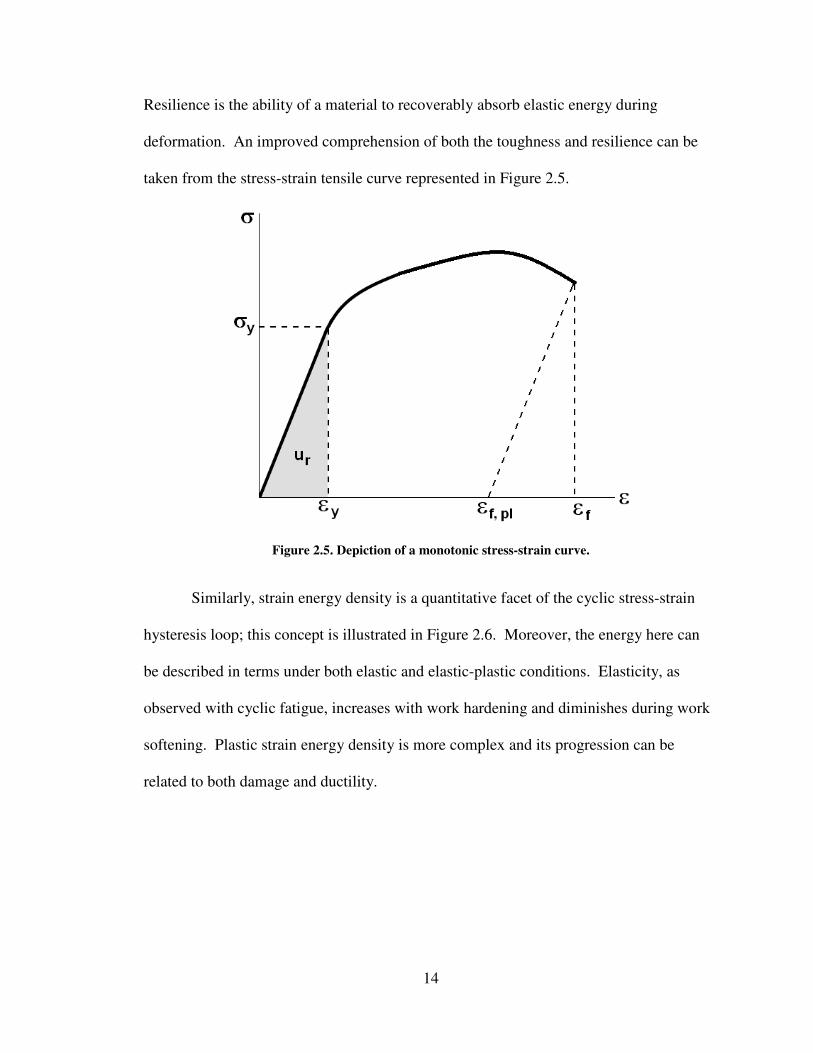
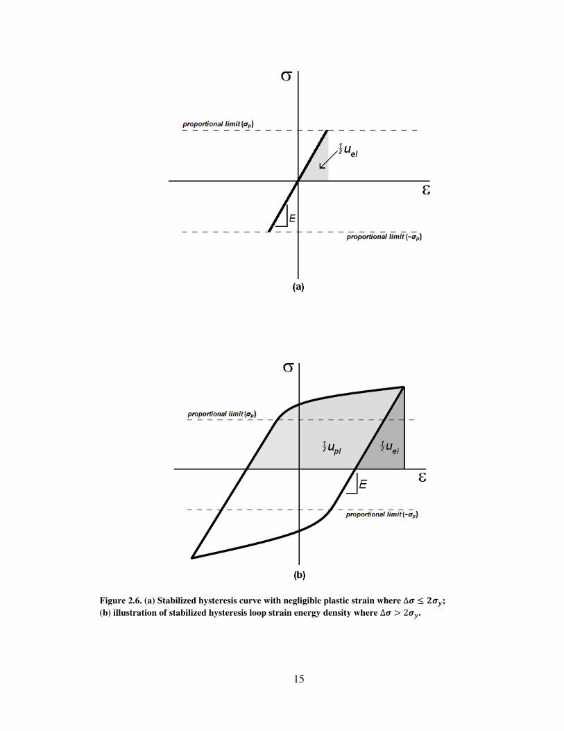
Similarly, strain energy density is a quantitative facet of the cyclic stress-strain
hysteresis loop; this concept is illustrated in Figure 2.6. Moreover, the energy here can
be described in terms under both elastic and elastic-plastic conditions. Elasticity, as
observed with cyclic fatigue, increases with work hardening and diminishes during work
softening. Plastic strain energy density is more complex and its progression can be
related to both damage and ductility.
15
Figure 2.6. (a) Stabilized hysteresis curve with negligible plastic strain where ∆5 � 657;
(b) illustration of stabilized hysteresis loop strain energy density where ∆5 � 257.
16
The total hysteresis energy density (ut), is defined as the sum of the elastic (uel) and
plastic (upl) hysteresis energies, i.e.,
�� $ ��� & � � (2.9)
Plastic strain energy density is evaluated as the area within the hysteresis loop;
furthermore, elastic strain energy density can be calculated by summing the two
triangular regions flanked by the outer parameter of the hysteresis loop and the abscissa.
An energetistic formulation can be devised to mathematically vindicate plastic strain
energy density,
� � $ 2+ �'�(�8,9
:�;<,9,� % �!"0
� (2.10)
While it has been habitually neglected in LCF lifetime prediction methods,
hysteresis stress (∆�), has proven to be a fundamental factor in the damage process.
Recently proposed hysteresis energy techniques incorporate this stress effectively. At
increased cyclic stresses, as realized in LCF and VLCF applications, fatigue damage is
primarily associated with plastic strain energy dissipation (Choe et al., 2006). Energy
measurements are generally calculated from either a half-life or cyclically stabilized
hysteresis loop and placed on energy versus life plots.
2.3. Anchor Points
An anchor point is a monotonic test datum point superimposed into a pre-existing
data set. This method allows for an enhanced qualitative fit of the strain-based curves
outside of the plastically inferior base data. The technique used to incorporate the anchor
point is analogous to the inclusion of other data: treat the point as a fatigue datum point
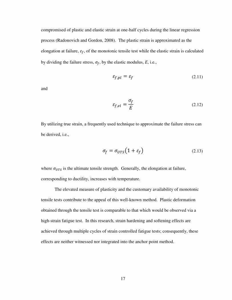
17
compromised of plastic and elastic strain at one-half cycles during the linear regression
process (Radonovich and Gordon, 2008). The plastic strain is approximated as the
elongation at failure, ��, of the monotonic tensile test while the elastic strain is calculated
by dividing the failure stress, ��, by the elastic modulus, E, i.e.,
��, � $ �� (2.11)
and
��,�� $ ��� (2.12)
By utilizing true strain, a frequently used technique to approximate the failure stress can
be derived, i.e.,
�� $ ����=1 & ��? (2.13)
where ���� is the ultimate tensile strength. Generally, the elongation at failure,
corresponding to ductility, increases with temperature.
The elevated measure of plasticity and the customary availability of monotonic
tensile tests contribute to the appeal of this well-known method. Plastic deformation
obtained through the tensile test is comparable to that which would be observed via a
high-strain fatigue test. In this research, strain hardening and softening effects are
achieved through multiple cycles of strain controlled fatigue tests; consequently, these
effects are neither witnessed nor integrated into the anchor point method.
18
2.4. Literature Review
2.4.1. Ni-base Superalloy Studies
One cannot thoroughly comprehend or attempt to predict fatigue behavior of a
material without an understanding of the microstructural evolution or damage
accumulation during mechanical loading. Balikci (1998) contributed a great deal of
effort in the study of IN738LC for temperatures ranging from 650°C-1250°C. Offering
both mechanical and material properties for numerous microstructures and strain rates,
this source is unsurpassed. The information provided by Balikci (1998) is most notably
valuable when assigning the proper heat treatment and precipitate size during IN738LC
processing; however, for this thesis the presented tensile data was imperative in deeming
the anchor point extrapolation incompatible. It should be noted, however, that neither
this nor any of the subsequent sources provided complete tensile curves. Another study
focused on IN738LC material attributes was developed by Bettge and coworkers (1995).
This source, although lacking fatigue data, further contributed to an understanding of
temperature dependency amongst assorted tensile-mechanical properties. Temperatures
investigated in this article range from 20°C-950°C.
Low cycle fatigue behavior of IN738LC in air and in vacuum is examined by
Marchionni and colleagues (1982) at 850°C. It is shown that cyclic tests performed in air
exhibit strain rate sensitivity and decreased cycles to failure as opposed to vacuum tests
where strain rate dependency was not observed. The strain rate applied in the study by
these researchers (1982) is identical to the testing parameters presented in this thesis.
Fatigue curves offered by Marchionni are analyzed by the Coffin-Manson equation.
19
In addition to the contributions made by Marchionni et al. (1982), several other
studies impart valuable data in which trends among LCF behavior of IN738LC can be
congregated. Jianting and Ranucci (1983) conducted strain-controlled LCF tests on
IN738LC specimens at room temperature; these experiments, at two different strain rates,
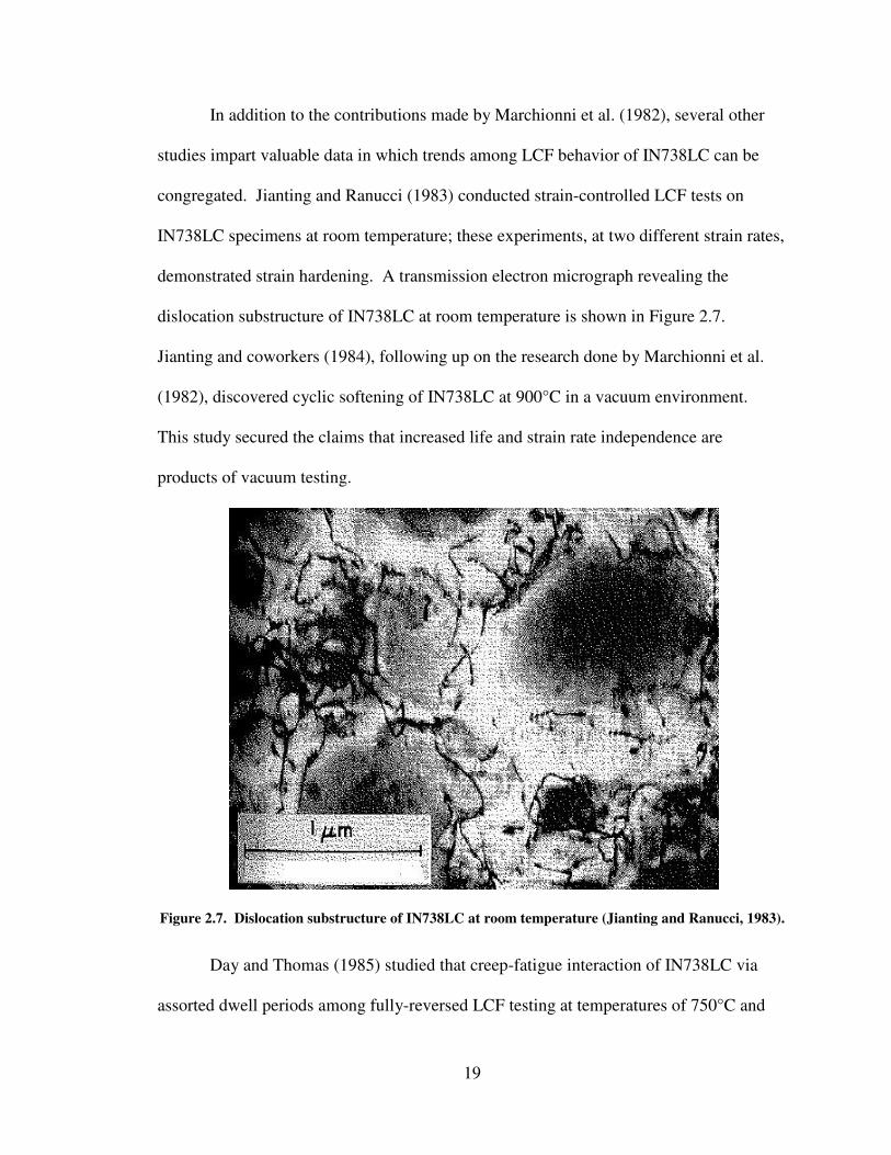
demonstrated strain hardening. A transmission electron micrograph revealing the
dislocation substructure of IN738LC at room temperature is shown in Figure 2.7.
Jianting and coworkers (1984), following up on the research done by Marchionni et al.
(1982), discovered cyclic softening of IN738LC at 900°C in a vacuum environment.
This study secured the claims that increased life and strain rate independence are
products of vacuum testing.
Figure 2.7. Dislocation substructure of IN738LC at room temperature (Jianting and Ranucci, 1983).
Day and Thomas (1985) studied that creep-fatigue interaction of IN738LC via
assorted dwell periods among fully-reversed LCF testing at temperatures of 750°C and
20
850°C. Although the chief conclusions found in this study are not entirely pertinent to
this research, functional data are presented. Fischmeister et al. (1986) analyzed damage
mechanism of IN738LC and detected monotonic strain softening in the material at
850°C. Another source of data which reveals strain softening effects at 850°C is offered
by Persson et al. (1986). This study also concluded that methods incorporating hysteresis
stress showed better correlation to fatigue data when compared to basic strain-life
predictions. An added supply of useful IN738LC data at 800°C is found in a report by
Matsuda and colleagues (1986). Germane strain-life data gathered from the preceding
sources are used to supplement this thesis.
Onodera and Ro (1986) provide an expansive view of LCF behavior based on
tensile properties among a variety of high-temperature Ni-base superalloys. Increased
ductility, as observed in IN738LC, was shown to have a positive effect on the fatigue life
when cycled through high stress regions where plastic deformation prevailed. Fatigue
lives of high strength alloys, as compared to low strength alloys, were superior during
reduced strain ranges. Fatigue cracks examined in this study were observed to initiate at
surface-connected grain boundaries and then propagate via both transgranular and
intergranular paths.
High temperature LCF of Inconel 713LC, akin to IN738LC, is studied and
inspected at the microstructural level by Petrenec and researchers (2007). Dislocation
structures developed through cyclic loading were examined by a transmission electron
microscope; these structures are related to the fatigue life and the cyclic plastic strain
response of the material. Persistent slip bands sited at increased strain ranges were
21
indicative of cyclic softening; this enhances perception of the behavior in the regime of
VLCF.
The information gathered in these material-based articles contributes to a
fundamental understanding of the microstructural evolution realized during loading and
the processes involved in characterizing material. A universal trend among this research
is the testing at room temperature followed by one or more increased temperature
experiments; this is executed to establish a foundation for comparison among other
materials. Although this realm of research does not always provide new methods of
estimation, an appreciation of damage beyond conventional formulae is achieved.
2.4.2. Existing Approximation Techniques
Various methods of estimating strain-life parameters have been established and
interminably assessed for surfeit amounts of different materials. Many of these
recognized techniques, principally comprised of alterations in the processes developed by
Manson (1965) and Ong (1993), were developed initially for steel alloys at room
temperature and have been proven incapable of representing fatigue trends for an
assortment of materials. Using several accepted methods of estimation and hundreds of
steel, titanium, and aluminum alloys, Meggiolaro and Castro (2004) along with Park and
Song (1995), demonstrate that a universal fatigue modeling method does not exist even at
room temperature. Meggiolaro and Castro (2004) stated, “All the presented estimates
should never be used in design, because for some materials, even the best methods may
result in life prediction errors of an order of magnitude.” Method amendments are
needed to characterize distinct alloy classes for design applications.
22
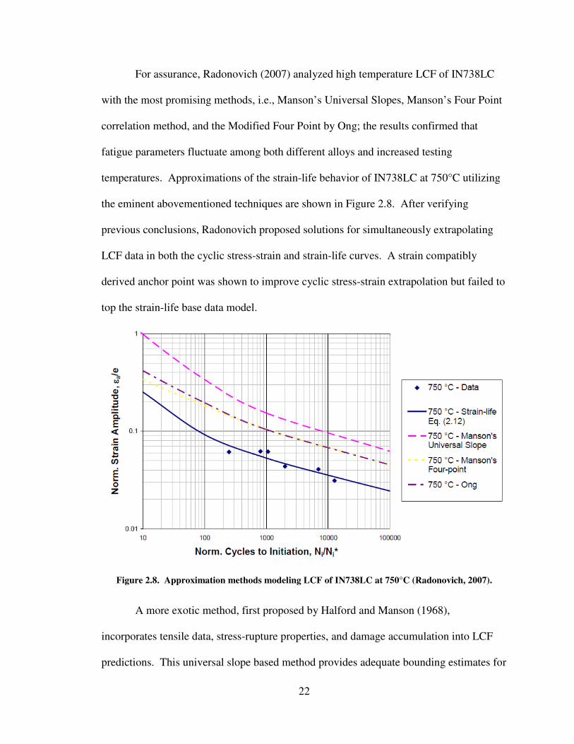
For assurance, Radonovich (2007) analyzed high temperature LCF of IN738LC
with the most promising methods, i.e., Manson’s Universal Slopes, Manson’s Four Point
correlation method, and the Modified Four Point by Ong; the results confirmed that
fatigue parameters fluctuate among both different alloys and increased testing
temperatures. Approximations of the strain-life behavior of IN738LC at 750°C utilizing
the eminent abovementioned techniques are shown in Figure 2.8. After verifying
previous conclusions, Radonovich proposed solutions for simultaneously extrapolating
LCF data in both the cyclic stress-strain and strain-life curves. A strain compatibly
derived anchor point was shown to improve cyclic stress-strain extrapolation but failed to
top the strain-life base data model.
Figure 2.8. Approximation methods modeling LCF of IN738LC at 750°C (Radonovich, 2007).
A more exotic method, first proposed by Halford and Manson (1968),
incorporates tensile data, stress-rupture properties, and damage accumulation into LCF
predictions. This universal slope based method provides adequate bounding estimates for
23
a variety of materials, including Ni-base alloys, at different test temperatures. Another
stress-rupture technique is provided by Danzer and Bressers (1986) and is designed
primarily for Ni-base alloys. These methods share three common drawbacks, (1) each
study concludes that the predictions are generally suitable for material selection purposes
only, (2) stress rupture properties are not always readily available for Ni-base
superalloys, and (3) creep damage mechanisms are not considered in this work.
As described earlier, hysteresis energy techniques exist to incorporate cyclic
stress for superior damage estimation. Such methods have been used to forecast life
predictions for LCF and thermo-mechanical fatigue (TMF) of Ni-base superalloys. Hyun
et al. (2006) studied in-phase and out-of-phase TMF of IN738LC; although the literature
concluded that lives were “satisfactorily predicted”, plastic strain energy was shown to
have a strong linear relationship. It should be noted that TMF prediction is more
complex than LCF and contributions by Hyun et al. (2006) are reputable. Low cycle
fatigue of direct aged Alloy 718, a Ni-base superalloy, was examined via plastic
hysteresis energy by Choe et al. (2006). The energy calculations for this superalloy did
not demonstrate a good linear fit. Trends in the accumulated hysteresis energy for
isothermal VLCF of IN738LC will be presented in this thesis.
Just as the majority of LCF estimation methods were first fabricated for steel,
aluminum, and titanium alloys, VLCF predictions are scarce for Ni-base superalloys.
The existing literature for VLCF estimation of these common alloys formulates complex
equations to capture data observed at low cycles (Kuroda, 2001; Tateishi et al., 2007;
Xue, 2008). Each of these papers has only an outlying tensile datum point located at 0.5
cycles to justify the curvature of the plastic data on the strain-life plot. Dufailly and
24
Lemaitre (1995) alike, whom studied VLCF of Inconel 718, have a deficient amount of
data to support inadequacies in the Coffin-Manson equation. There is no doubt that
accumulated damage mechanics models improve on incorporation of a tensile datum
point deviating from the linearity of the plastic data, but formulation of these equations is
not possible without ample amounts of LCF data dominated by plastic strain. Adjusting a
parameter obtained from a single tensile test may be sounder than guessing fracture
modes and damage accumulation at shorter lives.
Research delving directly into the fatigue of a component being cycled will
always exist. Three examples of these methods circumventing traditional material testing
for turbine blade fatigue examination are offered by Mazur et al. (2005), Troshchenko et
al. (2007), and Hou et al. (2009). The latter offers a life prediction model of an SC blade
that encompasses both HCF and LCF via elastic and crystallographic analyses,
respectively. Resolved shear stress amplitudes and maximum stresses, as opposed to
strains, are used to make lifetime approximations at relatively low cycles to failure.
An analysis performed by Troshchenko et al. (2007), in which the cyclic strength
and durability of turbine blades of various materials were studied, led to the existing
deduction that IN738 possesses superior fatigue properties. Mazur et al. (2005)
investigated the failure a turbine blade made of IN738LC; crack propagations within the
microstructure are evaluated and component replacement is recommended at the first site
of crack initiation, demonstrating the efficacy of the methods used in this thesis.
Life predictions of components are useful for design purposes, material
development, and risk mitigation (Wu et al., 2008). Though similar conclusions are
drawn from all dependable methods of lifetime prediction, the availability of data alters
25
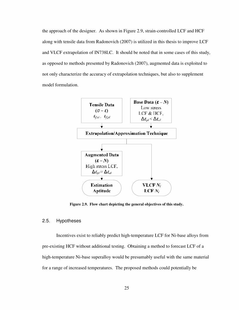
the approach of the designer. As shown in Figure 2.9, strain-controlled LCF and HCF
along with tensile data from Radonovich (2007) is utilized in this thesis to improve LCF
and VLCF extrapolation of IN738LC. It should be noted that in some cases of this study,
as opposed to methods presented by Radonovich (2007), augmented data is exploited to
not only characterize the accuracy of extrapolation techniques, but also to supplement
model formulation.
Figure 2.9. Flow chart depicting the general objectives of this study.
2.5. Hypotheses
Incentives exist to reliably predict high-temperature LCF for Ni-base alloys from
pre-existing HCF without additional testing. Obtaining a method to forecast LCF of a
high-temperature Ni-base superalloy would be presumably useful with the same material
for a range of increased temperatures. The proposed methods could potentially be
26
successful in modeling fatigue for other related Ni-base superalloys as well; e.g., IN738
and IN-713LC.
Once more, the focus of this research is to accurately replicate high-stress LCF
from available tensile and low-stress LCF data. With this goal in mind, the subsequent
suppositions will be determined in this study:
i) A monotonic anchor point derived from tensile data can effectively represent high-
stress LCF behavior on a strain-life diagram and may be used for extrapolation of
low-stress LCF data outside of its plastically inferior region.
ii) If scaling of the anchor point is needed to correlate with other high strain data, this
degree will be functional for all elevated temperatures. Once properly located anchor
points are determined for these increased temperatures, appropriate averaging may be
applied to broaden its candidacy.
iii) Scatter within the low-stress LCF plastic data is predominantly situated at longer
lives, i.e., low-stress localities. Apposite weighting of the plastic data at shorter lives
will allow for an improved linear regression of the Coffin-Manson equation.
iv) Elastic strain found throughout the LCF data is valid and does not need to be attuned
with anchor points or weighting techniques. Attempting such adjustments will lead to
flaws in Basquin’s equation.
v) Plastic strain energy density can be calculated from well-defined hysteresis loops,
where strain ranges are above one percent, and represented as functions of the mid-
life plastic strain range, ∆� �, and stress range, ∆�. These formulated functions can
be used to express energy density for less definitive loops and used to plot simple
trends that expand lifetime predictions and fatigue modeling of the material at a

27
variety of temperatures. Life may also be conservatively predicted using the product
energy of the mid-life stress range and plastic strain range, i.e. ∆�∆� �, as opposed to
the precise area within the hysteresis loop.
28
3. Approach
3.1. Experimentation
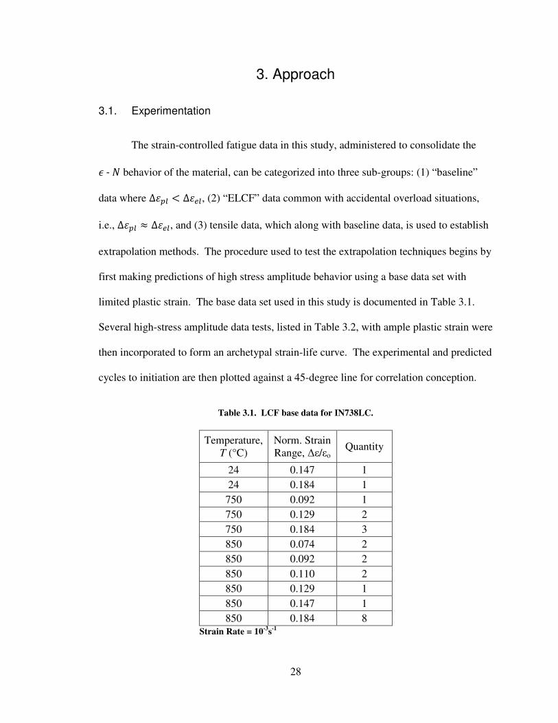
The strain-controlled fatigue data in this study, administered to consolidate the
@ - � behavior of the material, can be categorized into three sub-groups: (1) “baseline”
data where ∆� � � ∆���, (2) “ELCF” data common with accidental overload situations,
i.e., ∆� � � ∆���, and (3) tensile data, which along with baseline data, is used to establish
extrapolation methods. The procedure used to test the extrapolation techniques begins by
first making predictions of high stress amplitude behavior using a base data set with
limited plastic strain. The base data set used in this study is documented in Table 3.1.
Several high-stress amplitude data tests, listed in Table 3.2, with ample plastic strain were
then incorporated to form an archetypal strain-life curve. The experimental and predicted
cycles to initiation are then plotted against a 45-degree line for correlation conception.
Table 3.1. LCF base data for IN738LC.
Temperature,
T (°C)
Norm. Strain
Range, ∆ε/εo Quantity
24 0.147 1
24 0.184 1
750 0.092 1
750 0.129 2
750 0.184 3
850 0.074 2
850 0.092 2
850 0.110 2
850 0.129 1
850 0.147 1
850 0.184 8
Strain Rate = 10-3
s-1
29
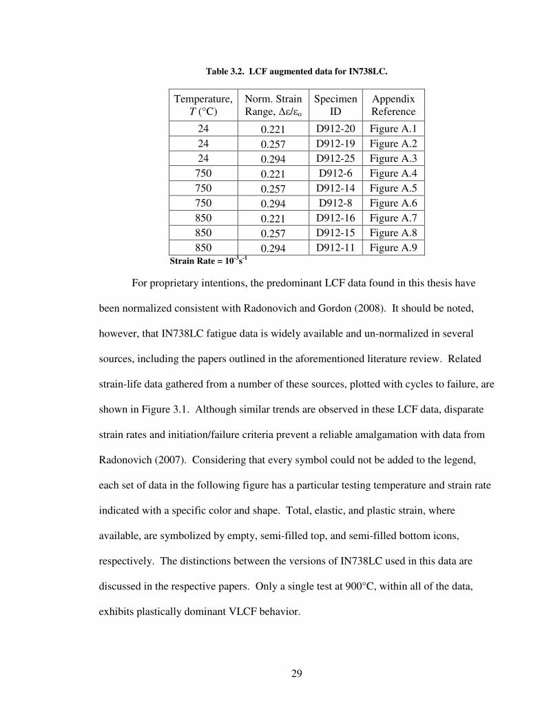
Table 3.2. LCF augmented data for IN738LC.
Temperature,
T (°C)
Norm. Strain
Range, ∆ε/εo
Specimen
ID
Appendix
Reference
24 0.221 D912-20 Figure A.1
24 0.257 D912-19 Figure A.2
24 0.294 D912-25 Figure A.3
750 0.221 D912-6 Figure A.4
750 0.257 D912-14 Figure A.5
750 0.294 D912-8 Figure A.6
850 0.221 D912-16 Figure A.7
850 0.257 D912-15 Figure A.8
850 0.294 D912-11 Figure A.9
Strain Rate = 10-3
s-1
For proprietary intentions, the predominant LCF data found in this thesis have
been normalized consistent with Radonovich and Gordon (2008). It should be noted,
however, that IN738LC fatigue data is widely available and un-normalized in several
sources, including the papers outlined in the aforementioned literature review. Related
strain-life data gathered from a number of these sources, plotted with cycles to failure, are
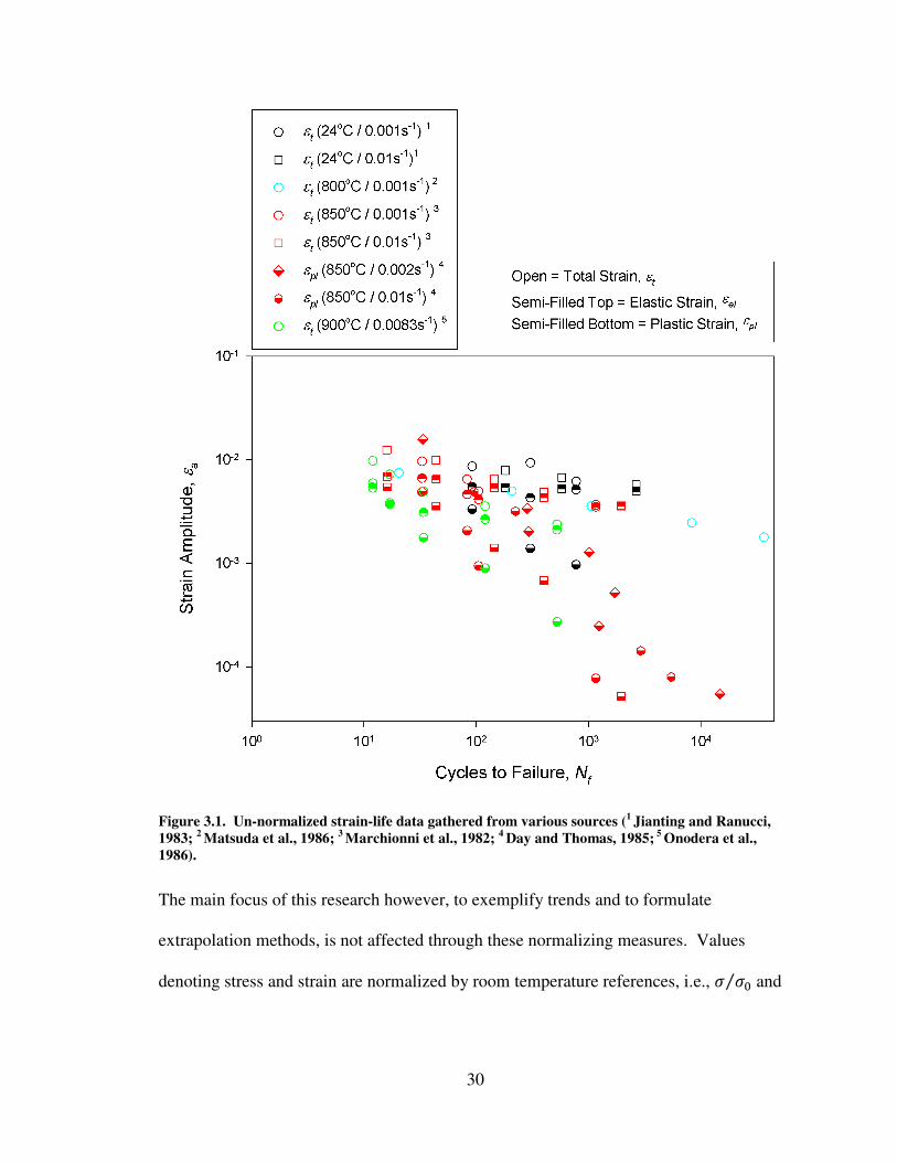
shown in Figure 3.1. Although similar trends are observed in these LCF data, disparate
strain rates and initiation/failure criteria prevent a reliable amalgamation with data from
Radonovich (2007). Considering that every symbol could not be added to the legend,
each set of data in the following figure has a particular testing temperature and strain rate
indicated with a specific color and shape. Total, elastic, and plastic strain, where
available, are symbolized by empty, semi-filled top, and semi-filled bottom icons,
respectively. The distinctions between the versions of IN738LC used in this data are
discussed in the respective papers. Only a single test at 900°C, within all of the data,
exhibits plastically dominant VLCF behavior.
30
Figure 3.1. Un-normalized strain-life data gathered from various sources (1 Jianting and Ranucci,
1983; 2 Matsuda et al., 1986;
3 Marchionni et al., 1982;
4 Day and Thomas, 1985;
5 Onodera et al.,
1986).
The main focus of this research however, to exemplify trends and to formulate
extrapolation methods, is not affected through these normalizing measures. Values
denoting stress and strain are normalized by room temperature references, i.e., � �.⁄ and
31
� �.⁄ , respectively. Cycles to initiation, Ni, have been divided through by an arbitrary
constant, Ni*.
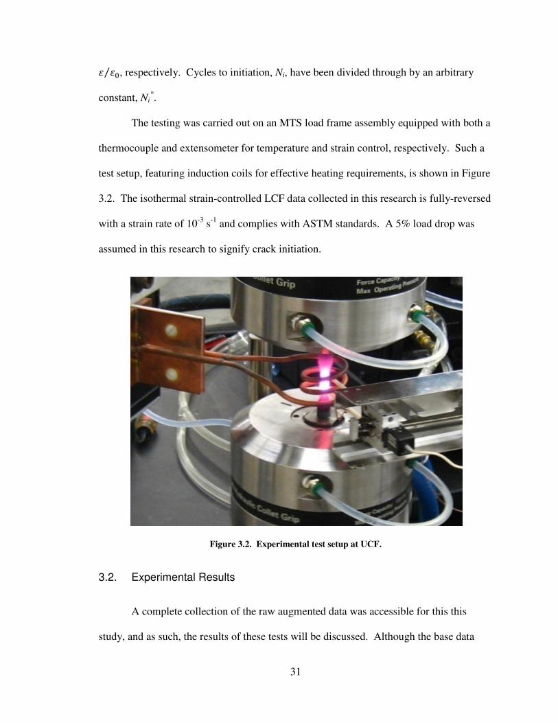
The testing was carried out on an MTS load frame assembly equipped with both a
thermocouple and extensometer for temperature and strain control, respectively. Such a
test setup, featuring induction coils for effective heating requirements, is shown in Figure
3.2. The isothermal strain-controlled LCF data collected in this research is fully-reversed
with a strain rate of 10-3
s-1
and complies with ASTM standards. A 5% load drop was
assumed in this research to signify crack initiation.
Figure 3.2. Experimental test setup at UCF.
3.2. Experimental Results
A complete collection of the raw augmented data was accessible for this this
study, and as such, the results of these tests will be discussed. Although the base data
32
used in the thesis were pulled together from past research, comparisons among the elastic
moduli and yield strengths at 750°C and 850°C deemed them compatible (Radonovich,
2007). From the augmented tests, stress versus cycles (stress histories) and cyclic stress-
strain curves (hysteresis loops) were exploited to determine strain hardening or softening
effects, crack initiations, and stabilization periods in conjunction with associated stress
and strain ranges.
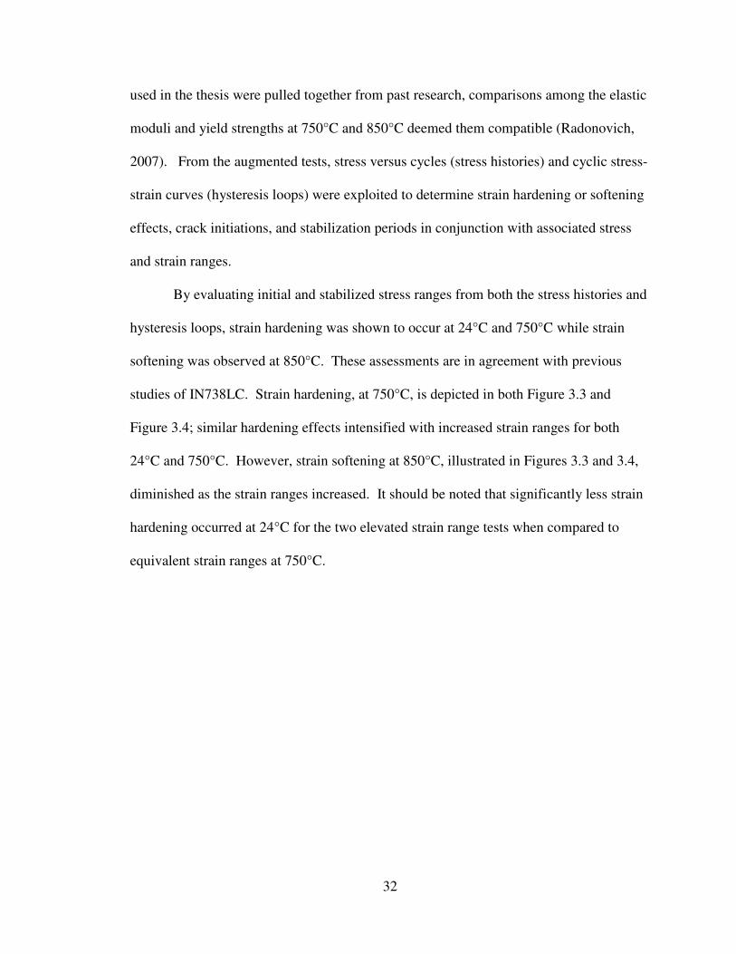
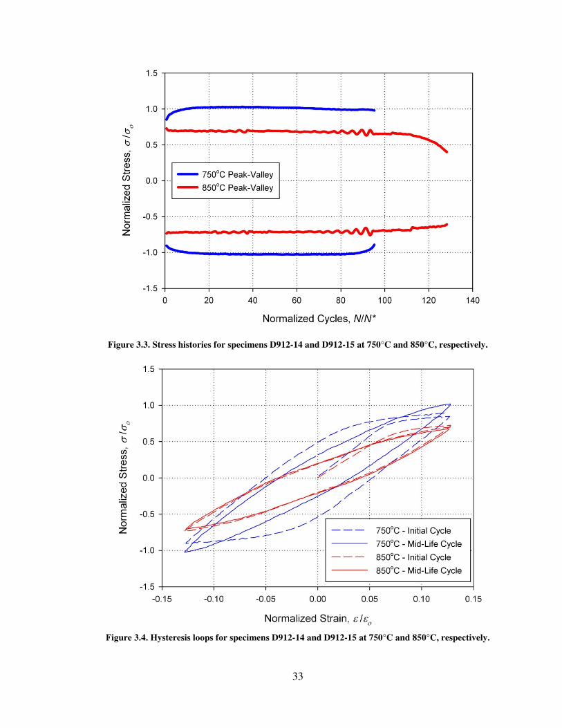
By evaluating initial and stabilized stress ranges from both the stress histories and
hysteresis loops, strain hardening was shown to occur at 24°C and 750°C while strain
softening was observed at 850°C. These assessments are in agreement with previous
studies of IN738LC. Strain hardening, at 750°C, is depicted in both Figure 3.3 and
Figure 3.4; similar hardening effects intensified with increased strain ranges for both
24°C and 750°C. However, strain softening at 850°C, illustrated in Figures 3.3 and 3.4,
diminished as the strain ranges increased. It should be noted that significantly less strain
hardening occurred at 24°C for the two elevated strain range tests when compared to
equivalent strain ranges at 750°C.
33
Figure 3.3. Stress histories for specimens D912-14 and D912-15 at 750°C and 850°C, respectively.
Figure 3.4. Hysteresis loops for specimens D912-14 and D912-15 at 750°C and 850°C, respectively.
34
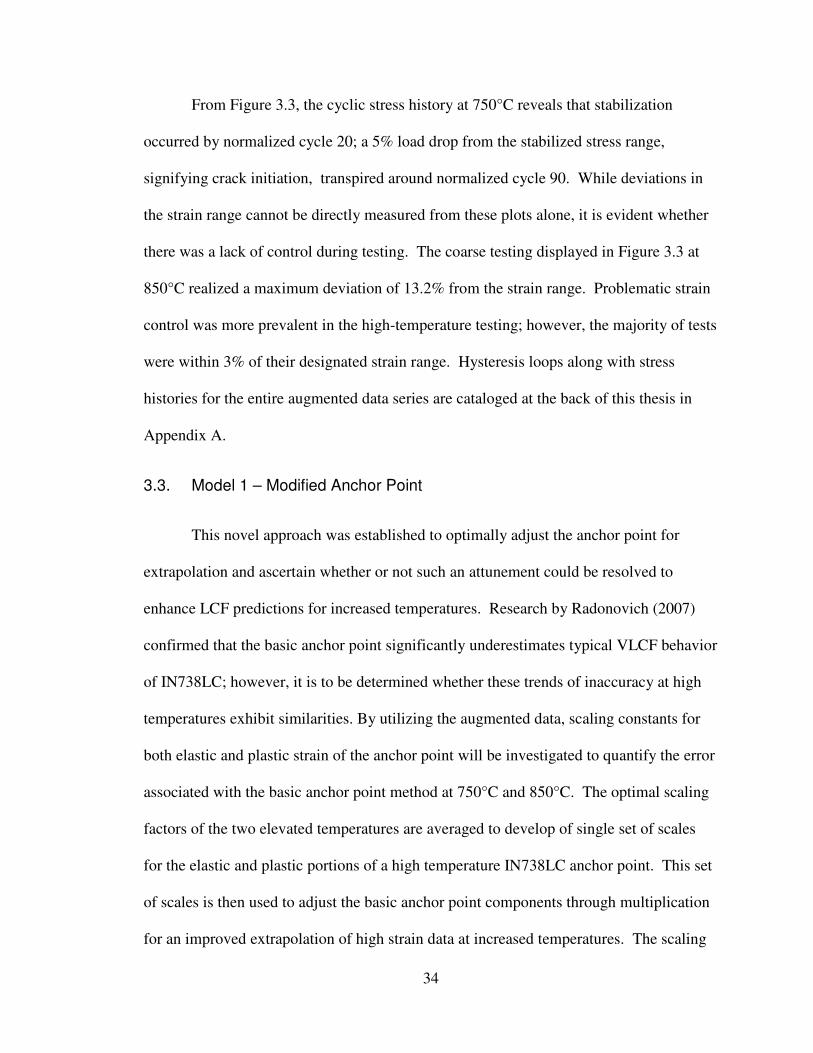
From Figure 3.3, the cyclic stress history at 750°C reveals that stabilization
occurred by normalized cycle 20; a 5% load drop from the stabilized stress range,
signifying crack initiation, transpired around normalized cycle 90. While deviations in
the strain range cannot be directly measured from these plots alone, it is evident whether
there was a lack of control during testing. The coarse testing displayed in Figure 3.3 at
850°C realized a maximum deviation of 13.2% from the strain range. Problematic strain
control was more prevalent in the high-temperature testing; however, the majority of tests
were within 3% of their designated strain range. Hysteresis loops along with stress
histories for the entire augmented data series are cataloged at the back of this thesis in
Appendix A.
3.3. Model 1 – Modified Anchor Point
This novel approach was established to optimally adjust the anchor point for
extrapolation and ascertain whether or not such an attunement could be resolved to
enhance LCF predictions for increased temperatures. Research by Radonovich (2007)
confirmed that the basic anchor point significantly underestimates typical VLCF behavior
of IN738LC; however, it is to be determined whether these trends of inaccuracy at high
temperatures exhibit similarities. By utilizing the augmented data, scaling constants for
both elastic and plastic strain of the anchor point will be investigated to quantify the error
associated with the basic anchor point method at 750°C and 850°C. The optimal scaling
factors of the two elevated temperatures are averaged to develop of single set of scales
for the elastic and plastic portions of a high temperature IN738LC anchor point. This set
of scales is then used to adjust the basic anchor point components through multiplication
for an improved extrapolation of high strain data at increased temperatures. The scaling
35
factors for the high-temperature anchor point adjustments used in this method are shown
in Table 3.3 along with a set of factors suitable for room temperature extrapolation. The
average factors displayed incorporate the 750°C and 850°C modifications only and are
not a function of the room temperature alteration. It should be noted again that this
method implements the augmented data to formulate the extrapolation process and
quantify errors associated with the basic anchor point. Using the augmented data in such
a manner has not yet been attempted.
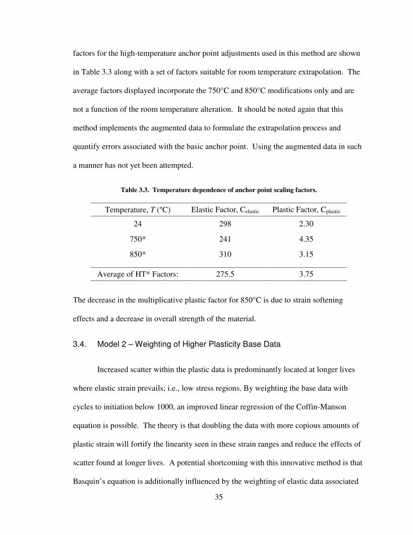
Table 3.3. Temperature dependence of anchor point scaling factors.
Temperature, T (°C) Elastic Factor, Celastic Plastic Factor, Cplastic
24 298 2.30
750* 241 4.35
850* 310 3.15
Average of HT* Factors: 275.5 3.75
The decrease in the multiplicative plastic factor for 850°C is due to strain softening
effects and a decrease in overall strength of the material.
3.4. Model 2 – Weighting of Higher Plasticity Base Data
Increased scatter within the plastic data is predominantly located at longer lives
where elastic strain prevails; i.e., low stress regions. By weighting the base data with
cycles to initiation below 1000, an improved linear regression of the Coffin-Manson
equation is possible. The theory is that doubling the data with more copious amounts of
plastic strain will fortify the linearity seen in these strain ranges and reduce the effects of
scatter found at longer lives. A potential shortcoming with this innovative method is that
Basquin’s equation is additionally influenced by the weighting of elastic data associated
36
with high plasticity. Considering that there are only two data points in the base data set
for 24°C, neither of which have increased plastic strain, this method is only applicable for
the 750°C and 850°C base data sets.
3.5. Model 3 – Original Basquin’s Equation Perpetuation
Attempting to extrapolate from plastically inferior data does not constitute
grounds for adjusting ample elastic strain data. This elastic strain data is valid and may
not need to be attuned with anchor points or weighting techniques; therefore, maintaining
Basquin’s equation from the original base data is proposed. The two preceding methods
can be corrected to utilize this concept:
1. When employing either the anchor point or modified version via the scaling
factors, simply do not include the elastic failure strain during the linear regression of
Basquin’s equation. In subsequent figures and graphs, this model will be displayed as
Model 3.1.
2. In attempting to weight the plastically superior base data, only include the plastic
data along with the cycles to initiation in the regression process; this will impede any
alterations in the elastic data. Such a technique will be denoted as Model 3.2.
3.6. Model 4 – Plastic Hysteresis Energy Density Trends
In this proposed method, the LCF energy density data of IN738LC, obtained from
mid-life hysteresis loops, are calculated in an attempt to identify the optimal ELCF
prediction approach for the candidate material. As previously mentioned, the stresses
realized during strain-controlled, fatigue testing are a major factor in damage accretion
and offer greater insight into the mechanisms of fatigue when incorporated into lifetime
37
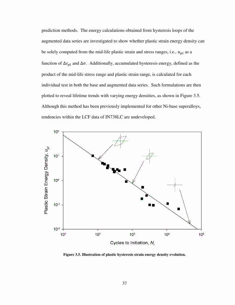
prediction methods. The energy calculations obtained from hysteresis loops of the
augmented data series are investigated to show whether plastic strain energy density can
be solely computed from the mid-life plastic strain and stress ranges, i.e., � � as a
function of ∆� � and ∆�. Additionally, accumulated hysteresis energy, defined as the
product of the mid-life stress range and plastic strain range, is calculated for each
individual test in both the base and augmented data series. Such formulations are then
plotted to reveal lifetime trends with varying energy densities, as shown in Figure 3.5.
Although this method has been previously implemented for other Ni-base superalloys,
tendencies within the LCF data of IN738LC are undeveloped.
Figure 3.5. Illustration of plastic hysteresis strain energy density evolution.
38
4. Model Results
4.1. Data Representation
Results presented in this section are displayed on a variety of graphs for an
enhanced conception of the models’ aptitudes. Low cycle fatigue strain data, as
mentioned earlier, are best exemplified on strain-life plots; this plotting technique, as
employed in this project, has been normalized for proprietary concerns. Each strain
amplitude, throughout all temperatures, has been normalized by a room temperature
reference, � �C⁄ . Maintaining consistent normalization, as opposed to implementing
individual constants, prevents biased shifts among the disparate temperatures.
Furthermore, an unvarying constant was used to normalize life; this also allows for
simultaneous linear shifts to occur. After failing to reliably correlate plastic mid-life
hysteresis energy density, from the defined area of each loop, to that of the related plastic
strain and stress ranges, it was decided that trends among the mid-life hysteresis energy,
∆�∆� �, would be investigated solitarily. This form of un-normalized energy is plotted
against normalized life, Ni/Ni*, as testament to its ability to forecast both VLCF and LCF
damage of IN738LC.
What remains to be determined is the strain-life-based model which can most
accurately predict high-stress amplitudes from existing tensile and base data.
Additionally, the potential of the energy-based model to represent this IN738LC data
remains indefinite. To improve model assessment, normalized experimental life is
plotted and compared to normalized predicted life. These plots feature a line of perfect
correlation along with supplementary lines signifying factors of both 1.5 and 2 scatter
39
band. This method of comparison, although entirely qualitative, is more effectual than
the Pearson product, R2, when evaluating the estimated bounds of each model. An R
2
value, known also as the moment correlation coefficient, measures the linear dependence
of two variables. Equivalent variables, however, are represented by a line with unity
slope. Accordingly, the R2 values are reliable only when they are derived from a pre-
determined function of unity slope; this was accomplished for the high temperature
extrapolation. The added effects of comparing correlations on the basis of life in lieu of
strain are discussed in Chapter 5. First, however, the model results will be evaluated.
4.2. Model Comparison
In this subsection, comparisons will be made between the models presented in
Chapter 3 and the related archetypal representations created from the base and augmented
data. For simplicity, the individual models have been abbreviated in several instances:
modified anchor point (Model 1 - MAP), weighting of the base data with increased
plasticity (Model 2 - WIP), original Basquin’s perpetuation of Model 1 (Model 3.1 –
OBMAP), original Basquin’s perpetuation of Model 2 (Model 3.2 – OBWIP), and trends
among plastic hysteresis energy (Model 4 – HEP). The strain-life base data model, using
strictly the base data, and the augmented data model, employing both the augmented and
base data, were created through linear regression as described in Chapter 2. The energy-
life models were created using, tensile, base, and augmented data to realize the tendencies
of each temperature. Table 4.1 displays the data sources employed into the models.
40
Table 4.1. Data sources for the individual models.
Model Tensile
Data Base Data
Augmented
Data
Base Data Model X � X
Augmented Data
Model X � �
Model 1 - MAP � � �
Model 2 - WIP X � X
Model 3.1 - OBMAP � � �
Model 3.2 -OBWIP X � X
Model 4 - HEP � � �
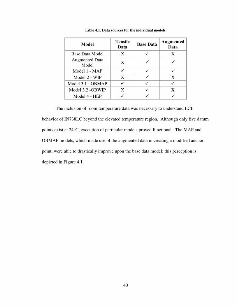
The inclusion of room temperature data was necessary to understand LCF
behavior of IN738LC beyond the elevated temperature region. Although only five datum
points exist at 24°C, execution of particular models proved functional. The MAP and
OBMAP models, which made use of the augmented data in creating a modified anchor
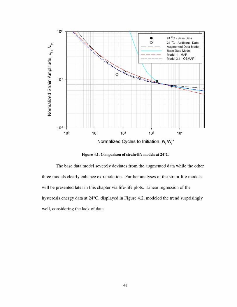
point, were able to drastically improve upon the base data model; this perception is
depicted in Figure 4.1.
41
Figure 4.1. Comparison of strain-life models at 24°C.
The base data model severely deviates from the augmented data while the other
three models clearly enhance extrapolation. Further analyses of the strain-life models
will be presented later in this chapter via life-life plots. Linear regression of the
hysteresis energy data at 24°C, displayed in Figure 4.2, modeled the trend surprisingly
well, considering the lack of data.
42
Figure 4.2. Linear regression of the hysteresis energy-life data at 24°C.
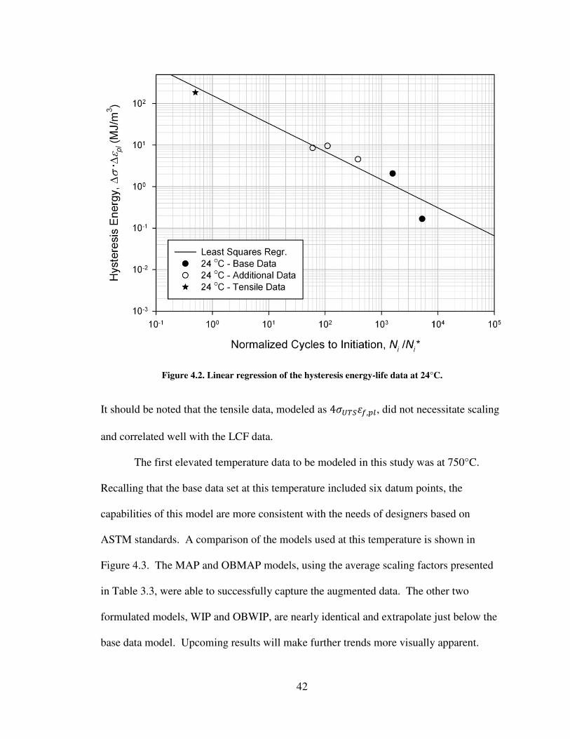
It should be noted that the tensile data, modeled as 4������, �, did not necessitate scaling
and correlated well with the LCF data.
The first elevated temperature data to be modeled in this study was at 750°C.
Recalling that the base data set at this temperature included six datum points, the
capabilities of this model are more consistent with the needs of designers based on
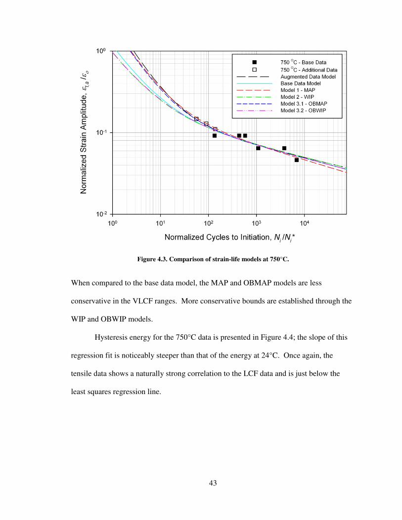
ASTM standards. A comparison of the models used at this temperature is shown in
Figure 4.3. The MAP and OBMAP models, using the average scaling factors presented
in Table 3.3, were able to successfully capture the augmented data. The other two
formulated models, WIP and OBWIP, are nearly identical and extrapolate just below the
base data model. Upcoming results will make further trends more visually apparent.
43
Figure 4.3. Comparison of strain-life models at 750°C.
When compared to the base data model, the MAP and OBMAP models are less
conservative in the VLCF ranges. More conservative bounds are established through the
WIP and OBWIP models.
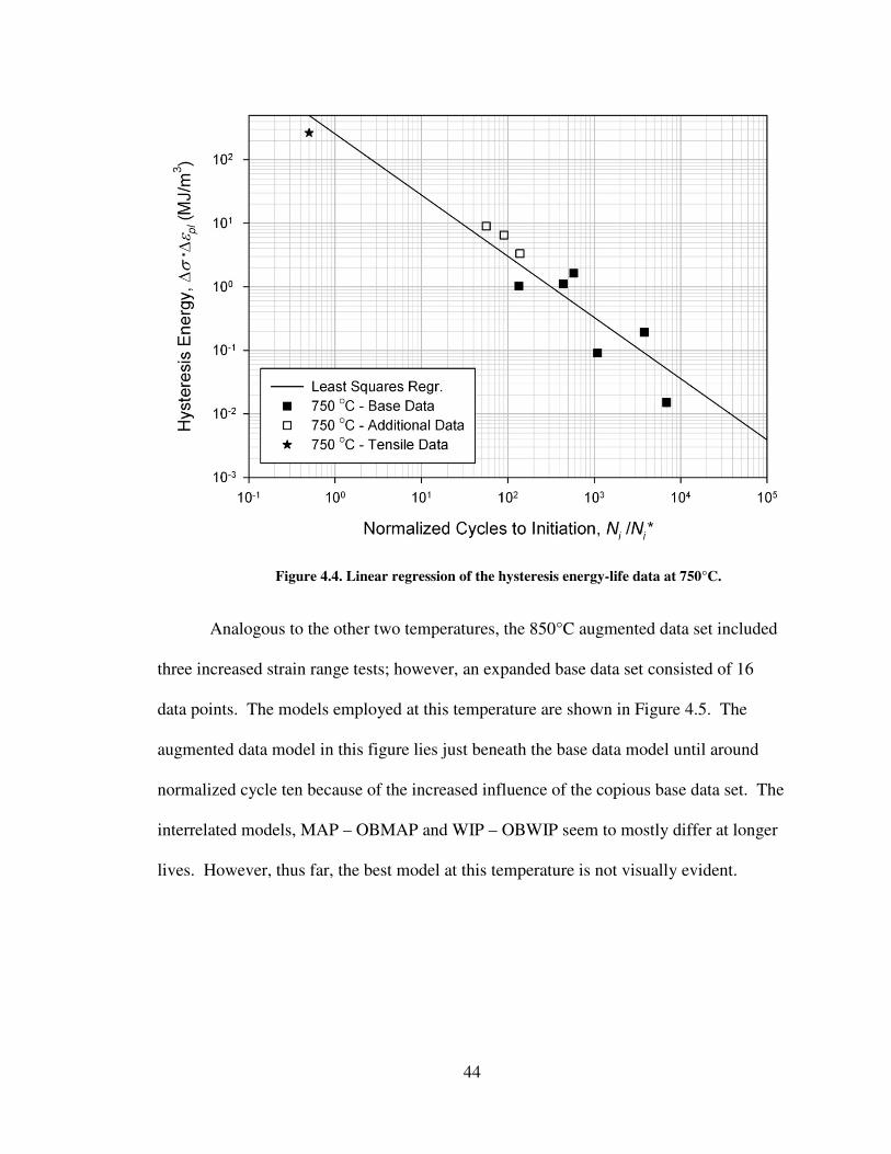
Hysteresis energy for the 750°C data is presented in Figure 4.4; the slope of this
regression fit is noticeably steeper than that of the energy at 24°C. Once again, the
tensile data shows a naturally strong correlation to the LCF data and is just below the
least squares regression line.
44
Figure 4.4. Linear regression of the hysteresis energy-life data at 750°C.
Analogous to the other two temperatures, the 850°C augmented data set included
three increased strain range tests; however, an expanded base data set consisted of 16
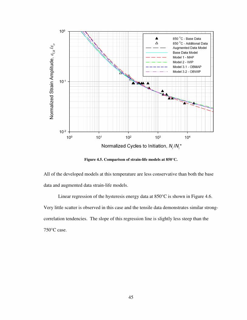
data points. The models employed at this temperature are shown in Figure 4.5. The
augmented data model in this figure lies just beneath the base data model until around
normalized cycle ten because of the increased influence of the copious base data set. The
interrelated models, MAP – OBMAP and WIP – OBWIP seem to mostly differ at longer
lives. However, thus far, the best model at this temperature is not visually evident.
45
Figure 4.5. Comparison of strain-life models at 850°C.
All of the developed models at this temperature are less conservative than both the base
data and augmented data strain-life models.
Linear regression of the hysteresis energy data at 850°C is shown in Figure 4.6.
Very little scatter is observed in this case and the tensile data demonstrates similar strong-
correlation tendencies. The slope of this regression line is slightly less steep than the
750°C case.
46
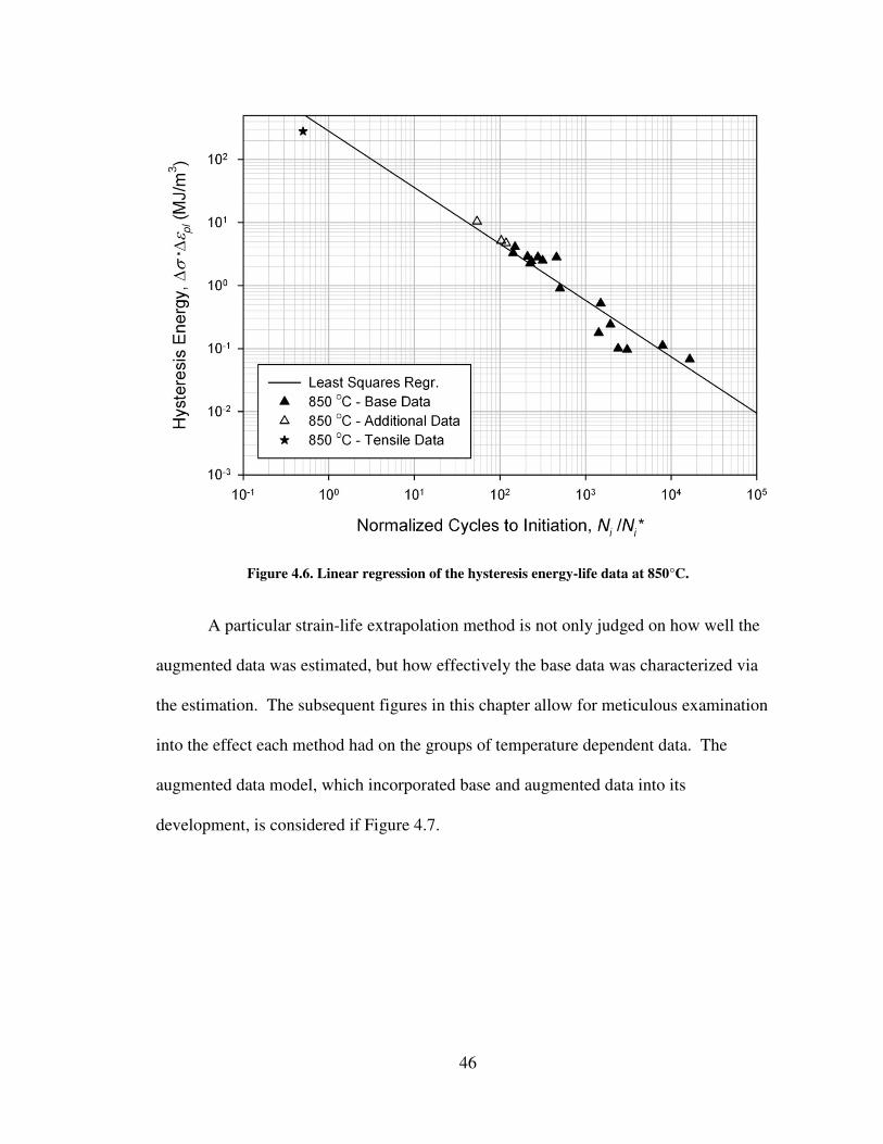
Figure 4.6. Linear regression of the hysteresis energy-life data at 850°C.
A particular strain-life extrapolation method is not only judged on how well the
augmented data was estimated, but how effectively the base data was characterized via
the estimation. The subsequent figures in this chapter allow for meticulous examination
into the effect each method had on the groups of temperature dependent data. The
augmented data model, which incorporated base and augmented data into its
development, is considered if Figure 4.7.
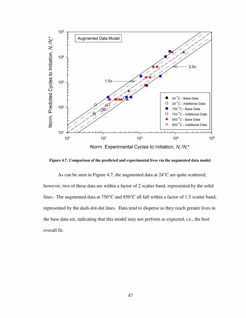
47
Figure 4.7. Comparison of the predicted and experimental lives via the augmented data model.
As can be seen in Figure 4.7, the augmented data at 24°C are quite scattered;
however, two of these data are within a factor of 2 scatter band, represented by the solid
lines. The augmented data at 750°C and 850°C all fall within a factor of 1.5 scatter band,
represented by the dash-dot-dot lines. Data tend to disperse as they reach greater lives in
the base data set, indicating that this model may not perform as expected, i.e., the best
overall fit.
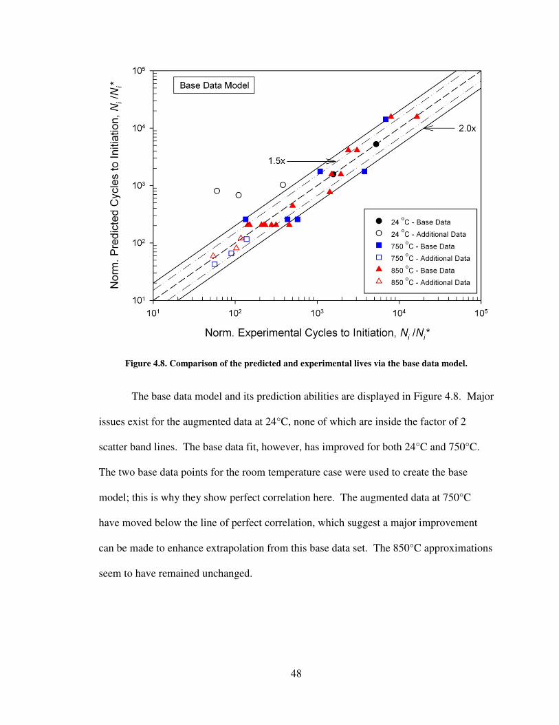
48
Figure 4.8. Comparison of the predicted and experimental lives via the base data model.
The base data model and its prediction abilities are displayed in Figure 4.8. Major
issues exist for the augmented data at 24°C, none of which are inside the factor of 2
scatter band lines. The base data fit, however, has improved for both 24°C and 750°C.
The two base data points for the room temperature case were used to create the base
model; this is why they show perfect correlation here. The augmented data at 750°C
have moved below the line of perfect correlation, which suggest a major improvement
can be made to enhance extrapolation from this base data set. The 850°C approximations
seem to have remained unchanged.
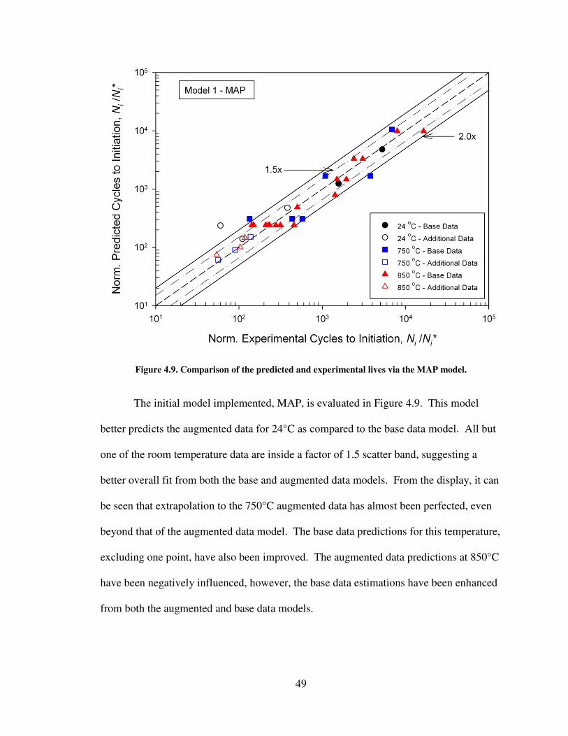
49
Figure 4.9. Comparison of the predicted and experimental lives via the MAP model.
The initial model implemented, MAP, is evaluated in Figure 4.9. This model
better predicts the augmented data for 24°C as compared to the base data model. All but
one of the room temperature data are inside a factor of 1.5 scatter band, suggesting a
better overall fit from both the base and augmented data models. From the display, it can
be seen that extrapolation to the 750°C augmented data has almost been perfected, even
beyond that of the augmented data model. The base data predictions for this temperature,
excluding one point, have also been improved. The augmented data predictions at 850°C
have been negatively influenced, however, the base data estimations have been enhanced
from both the augmented and base data models.
50
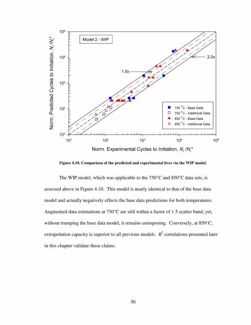
Figure 4.10. Comparison of the predicted and experimental lives via the WIP model.
The WIP model, which was applicable to the 750°C and 850°C data sets, is
assessed above in Figure 4.10. This model is nearly identical to that of the base data
model and actually negatively effects the base data predictions for both temperatures.
Augmented data estimations at 750°C are still within a factor of 1.5 scatter band; yet,
without trumping the base data model, it remains unimposing. Conversely, at 850°C,
extrapolation capacity is superior to all previous models. R2 correlations presented later
in this chapter validate these claims.
51
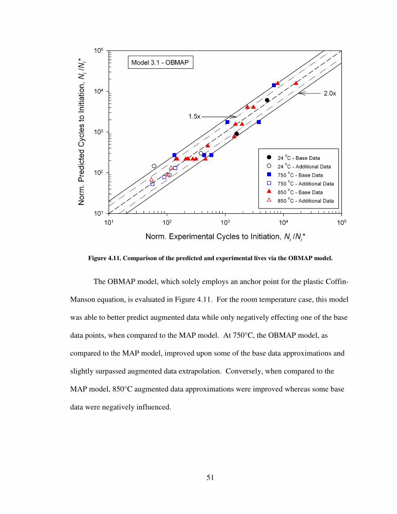
Figure 4.11. Comparison of the predicted and experimental lives via the OBMAP model.
The OBMAP model, which solely employs an anchor point for the plastic Coffin-
Manson equation, is evaluated in Figure 4.11. For the room temperature case, this model
was able to better predict augmented data while only negatively effecting one of the base
data points, when compared to the MAP model. At 750°C, the OBMAP model, as
compared to the MAP model, improved upon some of the base data approximations and
slightly surpassed augmented data extrapolation. Conversely, when compared to the
MAP model, 850°C augmented data approximations were improved whereas some base
data were negatively influenced.
52
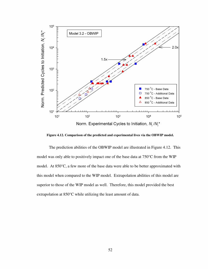
Figure 4.12. Comparison of the predicted and experimental lives via the OBWIP model.
The prediction abilities of the OBWIP model are illustrated in Figure 4.12. This
model was only able to positively impact one of the base data at 750°C from the WIP
model. At 850°C, a few more of the base data were able to be better approximated with
this model when compared to the WIP model. Extrapolation abilities of this model are
superior to those of the WIP model as well. Therefore, this model provided the best
extrapolation at 850°C while utilizing the least amount of data.
53
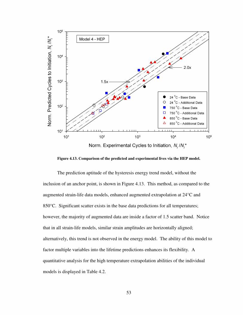
Figure 4.13. Comparison of the predicted and experimental lives via the HEP model.
The prediction aptitude of the hysteresis energy trend model, without the
inclusion of an anchor point, is shown in Figure 4.13. This method, as compared to the
augmented strain-life data models, enhanced augmented extrapolation at 24°C and
850°C. Significant scatter exists in the base data predictions for all temperatures;
however, the majority of augmented data are inside a factor of 1.5 scatter band. Notice
that in all strain-life models, similar strain amplitudes are horizontally aligned;
alternatively, this trend is not observed in the energy model. The ability of this model to
factor multiple variables into the lifetime predictions enhances its flexibility. A
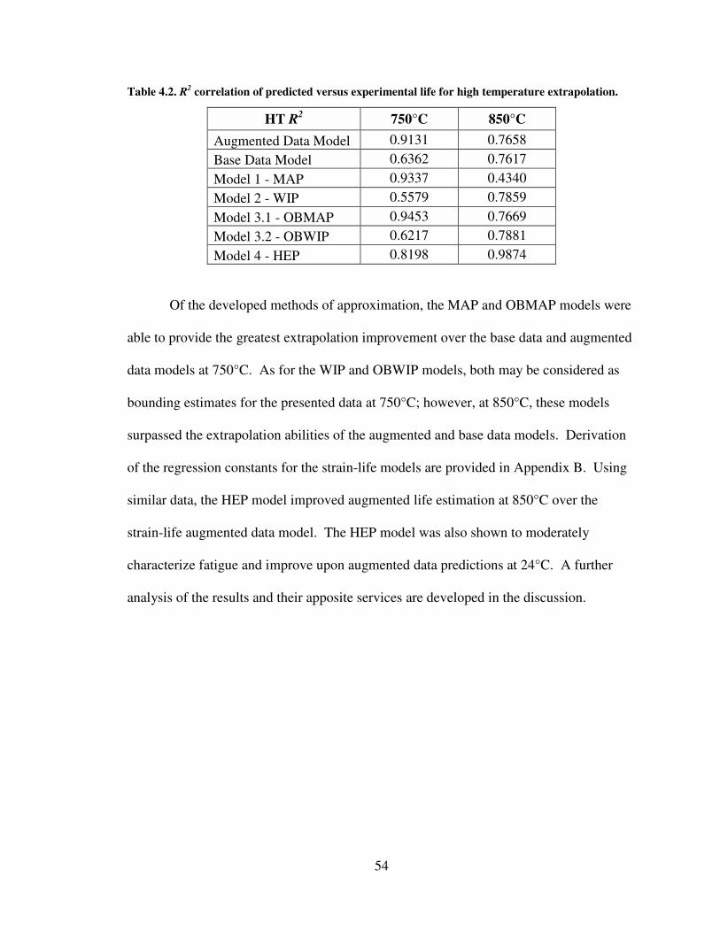
quantitative analysis for the high temperature extrapolation abilities of the individual
models is displayed in Table 4.2.
54
Table 4.2. R2 correlation of predicted versus experimental life for high temperature extrapolation.
HT R2 750°C 850°C
Augmented Data Model 0.9131 0.7658
Base Data Model 0.6362 0.7617
Model 1 - MAP 0.9337 0.4340
Model 2 - WIP 0.5579 0.7859
Model 3.1 - OBMAP 0.9453 0.7669
Model 3.2 - OBWIP 0.6217 0.7881
Model 4 - HEP 0.8198 0.9874
Of the developed methods of approximation, the MAP and OBMAP models were
able to provide the greatest extrapolation improvement over the base data and augmented
data models at 750°C. As for the WIP and OBWIP models, both may be considered as
bounding estimates for the presented data at 750°C; however, at 850°C, these models
surpassed the extrapolation abilities of the augmented and base data models. Derivation
of the regression constants for the strain-life models are provided in Appendix B. Using
similar data, the HEP model improved augmented life estimation at 850°C over the
strain-life augmented data model. The HEP model was also shown to moderately
characterize fatigue and improve upon augmented data predictions at 24°C. A further
analysis of the results and their apposite services are developed in the discussion.
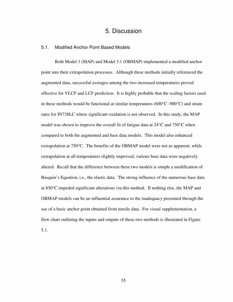
55
5. Discussion
5.1. Modified Anchor Point Based Models
Both Model 1 (MAP) and Model 3.1 (OBMAP) implemented a modified anchor
point into their extrapolation processes. Although these methods initially referenced the
augmented data, successful averages among the two increased temperatures proved
effective for VLCF and LCF prediction. It is highly probable that the scaling factors used
in these methods would be functional at similar temperatures (600°C -900°C) and strain
rates for IN738LC where significant oxidation is not observed. In this study, the MAP
model was shown to improve the overall fit of fatigue data at 24°C and 750°C when
compared to both the augmented and base data models. This model also enhanced
extrapolation at 750°C. The benefits of the OBMAP model were not as apparent; while
extrapolation at all temperatures slightly improved, various base data were negatively
altered. Recall that the difference between these two models is simple a modification of
Basquin’s Equation, i.e., the elastic data. The strong influence of the numerous base data
at 850°C impeded significant alterations via this method. If nothing else, the MAP and
OBMAP models can be an influential assurance to the inadequacy presented through the
use of a basic anchor point obtained from tensile data. For visual supplementation, a
flow chart outlining the inputs and outputs of these two methods is illustrated in Figure
5.1.
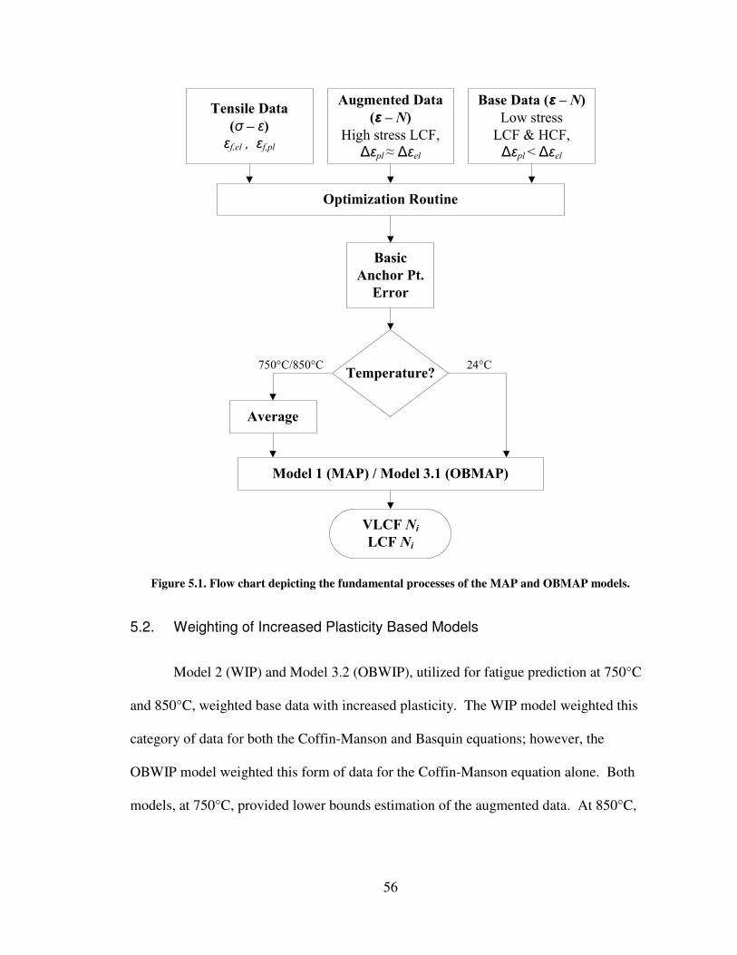
56
Augmented Data
(ε – N)
High stress LCF,
∆εpl≈ ∆εel
Base Data (ε – N)
Low stress
LCF & HCF,
∆εpl< ∆εel
Tensile Data
(σ – ε)
εf,el , εf,pl
Optimization Routine
Basic
Anchor Pt.
Error
Temperature?24°C750°C/850°C
Average
Model 1 (MAP) / Model 3.1 (OBMAP)
VLCF NiLCF Ni
Figure 5.1. Flow chart depicting the fundamental processes of the MAP and OBMAP models.
5.2. Weighting of Increased Plasticity Based Models
Model 2 (WIP) and Model 3.2 (OBWIP), utilized for fatigue prediction at 750°C
and 850°C, weighted base data with increased plasticity. The WIP model weighted this
category of data for both the Coffin-Manson and Basquin equations; however, the
OBWIP model weighted this form of data for the Coffin-Manson equation alone. Both
models, at 750°C, provided lower bounds estimation of the augmented data. At 850°C,
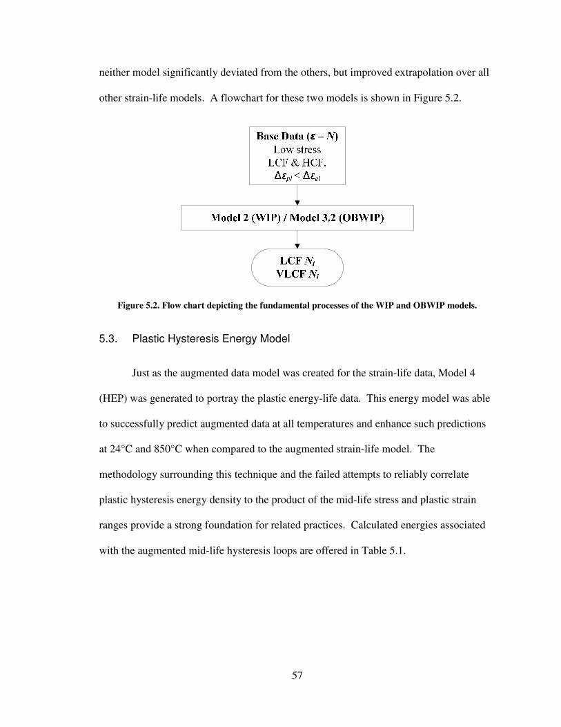
57
neither model significantly deviated from the others, but improved extrapolation over all
other strain-life models. A flowchart for these two models is shown in Figure 5.2.
Figure 5.2. Flow chart depicting the fundamental processes of the WIP and OBWIP models.
5.3. Plastic Hysteresis Energy Model
Just as the augmented data model was created for the strain-life data, Model 4
(HEP) was generated to portray the plastic energy-life data. This energy model was able
to successfully predict augmented data at all temperatures and enhance such predictions
at 24°C and 850°C when compared to the augmented strain-life model. The
methodology surrounding this technique and the failed attempts to reliably correlate
plastic hysteresis energy density to the product of the mid-life stress and plastic strain
ranges provide a strong foundation for related practices. Calculated energies associated
with the augmented mid-life hysteresis loops are offered in Table 5.1.
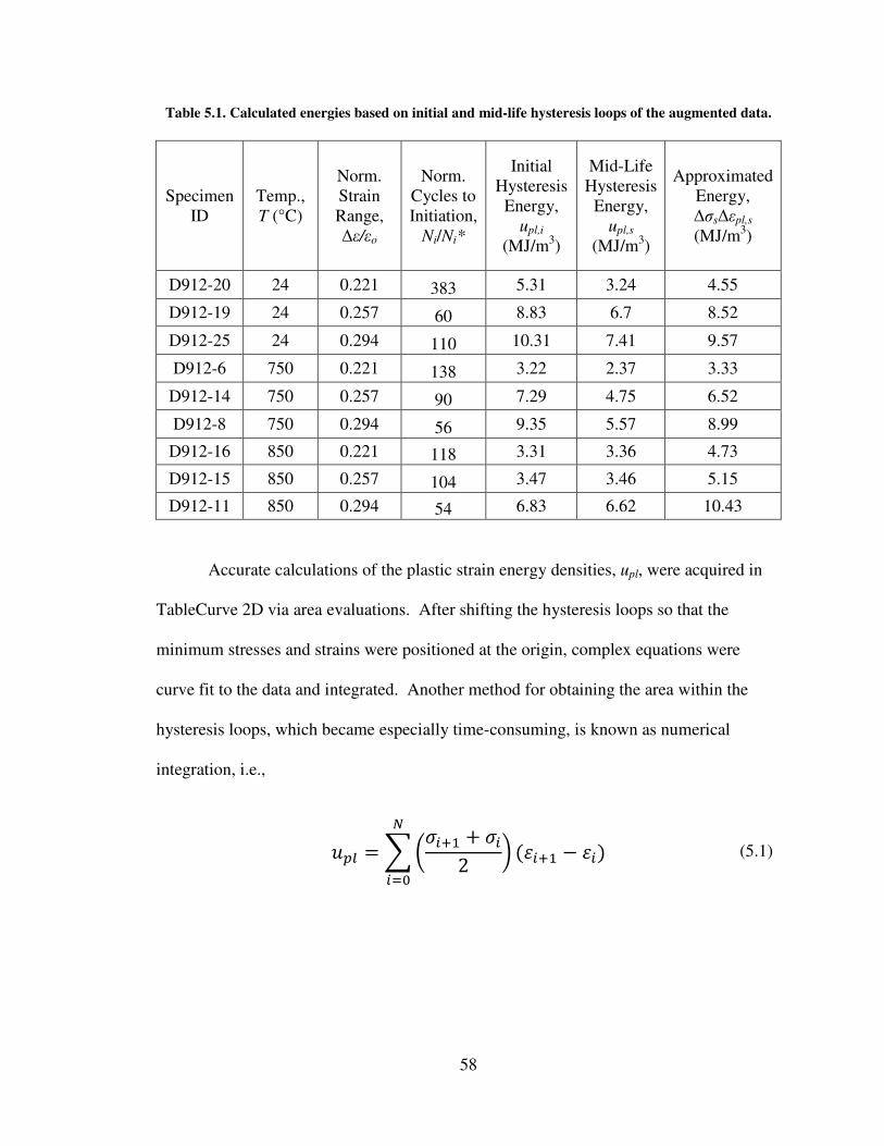
58
Table 5.1. Calculated energies based on initial and mid-life hysteresis loops of the augmented data.
Specimen
ID
Temp.,
T (°C)
Norm.
Strain
Range,
∆ε/εo
Norm.
Cycles to
Initiation,
Ni/Ni*
Initial
Hysteresis
Energy,
upl,i
(MJ/m3)
Mid-Life
Hysteresis
Energy,
upl,s
(MJ/m3)
Approximated
Energy,
∆σs∆εpl,s
(MJ/m3)
D912-20 24 0.221 383 5.31 3.24 4.55
D912-19 24 0.257 60 8.83 6.7 8.52
D912-25 24 0.294 110 10.31 7.41 9.57
D912-6 750 0.221 138 3.22 2.37 3.33
D912-14 750 0.257 90 7.29 4.75 6.52
D912-8 750 0.294 56 9.35 5.57 8.99
D912-16 850 0.221 118 3.31 3.36 4.73
D912-15 850 0.257 104 3.47 3.46 5.15
D912-11 850 0.294 54 6.83 6.62 10.43
Accurate calculations of the plastic strain energy densities, upl, were acquired in
TableCurve 2D via area evaluations. After shifting the hysteresis loops so that the
minimum stresses and strains were positioned at the origin, complex equations were
curve fit to the data and integrated. Another method for obtaining the area within the
hysteresis loops, which became especially time-consuming, is known as numerical
integration, i.e.,
� � $ EF��G/ & ��2 H '��G/ % ��(
I
�J. (5.1)
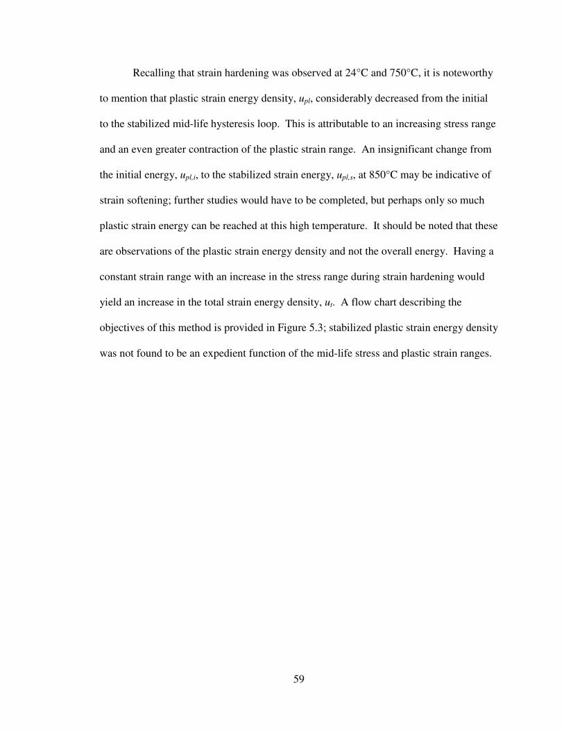
59
Recalling that strain hardening was observed at 24°C and 750°C, it is noteworthy
to mention that plastic strain energy density, upl, considerably decreased from the initial
to the stabilized mid-life hysteresis loop. This is attributable to an increasing stress range
and an even greater contraction of the plastic strain range. An insignificant change from
the initial energy, upl,i, to the stabilized strain energy, upl,s, at 850°C may be indicative of
strain softening; further studies would have to be completed, but perhaps only so much
plastic strain energy can be reached at this high temperature. It should be noted that these
are observations of the plastic strain energy density and not the overall energy. Having a
constant strain range with an increase in the stress range during strain hardening would
yield an increase in the total strain energy density, ut. A flow chart describing the
objectives of this method is provided in Figure 5.3; stabilized plastic strain energy density
was not found to be an expedient function of the mid-life stress and plastic strain ranges.
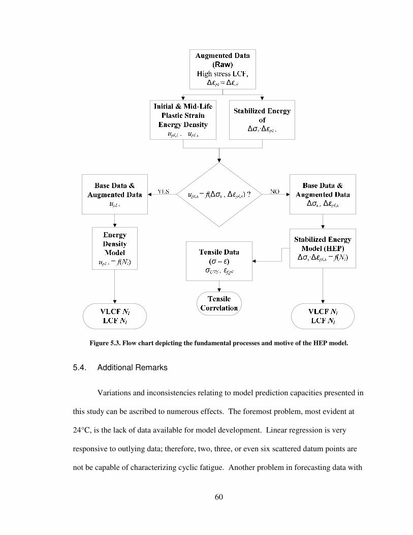
60
Figure 5.3. Flow chart depicting the fundamental processes and motive of the HEP model.
5.4. Additional Remarks
Variations and inconsistencies relating to model prediction capacities presented in
this study can be ascribed to numerous effects. The foremost problem, most evident at
24°C, is the lack of data available for model development. Linear regression is very
responsive to outlying data; therefore, two, three, or even six scattered datum points are
not be capable of characterizing cyclic fatigue. Another problem in forecasting data with
61
the strain-life curves, which is more difficult to circumvent, is the differences in lives of
data with identical strain amplitudes. Data in this study, at 1.0% strain ranges, had
differences in life to initiation above 200 cycles. Other data, with strain ranges of 0.4%,
had differences in lives above 10,000 cycles. Although these errors are common, they
must be considered when evaluating prediction models. An additional drawback, which
does not influence extrapolation as much as it does overall prediction, is described in
Figure 5.4.
Figure 5.4. Shortcoming of increased life predictions with the strain-life curve.
This effect, although not as prevalent in high strain amplitude regions, can cause strain-
life approximations to be very sensitive at increased life and should be taken into
consideration when comparing predicted lives or strain amplitudes. The distribution of

62
this low stress data also contains scatter because environmental effects are further
established. Extrapolation abilities are not impacted through these limitations because
data in this region are known prior to model development. As the curve approaches unity
slope, the differences in error between strain and life diminish. Further cautions and
summations of these models are presented in Chapter 6.
63
6. Conclusions
The intent of this study is to accurately characterize VLCF and high-stress LCF
from existing HCF, low-stress LCF, and tensile data. This objective is realized through
several novel approaches. Model 1 (MAP) and Model 3.1 (OBMAP), although aided by
high-stress data, improve upon extrapolation from the augmented data models at 24°C
and 750°C. Model 2 (WIP) and Model 3.2 (OBWIP) are able to surpass the extrapolation
abilities of all other strain-life methods at 850°C. Model 4 (HEP), the energy-life
approach, is able to adequately approximate the high-stress augmented data and
demonstrate an improved correlation with tensile data; these observations suggest that
energy-factoring methods are most suitable for VLCF behavior. The data used in this
study is in accord with results presented in other research; therefore, the products of this
project may be exercised with conviction. Comparing predicted life and experimental
life provides an additional factor of safety as opposed to comparisons between predicted
and experimental strains; this concept was illustrated earlier in Chapter 5.
In certain instances, the models offered in this study may achieve different results.
The inclusion of a modified anchor point significantly improved extrapolation to high-
stress regions at 24°C and 750°C; yet, the scaling factors in this research may not relate
accordingly to dissimilar data. Conversely, if less scatter is observed in particularly high-
plastic localities of data, the employment of either the WIP or OBWIP models may yield
superior results at a variety of temperatures. Together, all of the models presented can be
functional for different aspects of material testing. The ability to simply provide
bounding estimates is exceptionally useful for both material selection purposes and
construction of test matrices prior to experimentation.

64
As a caution, it should be noted that these methods are not intended for material
characterization in the place of ample quantities of valid fatigue data. The techniques
employed here demonstrate enhanced prediction capabilities; however, when attempting
to forecast fatigue, standard practices should always be performed first.
65
7. Future Work
With completion of this exploration, tremendous opportunities exist to advance
the prospect of accurately characterizing extensive ranges of fatigue with minimum data.
Results realized in this study may also be improved through further investigations.
Primarily, attainment of increased quantities of valid data must be pursued in order to
fully comprehend the benefits of the methods suggested in this research; a design quality
level of data was only offered at one temperature, 850°C.
Although extrapolation and prediction techniques are formulated for such reduced
amounts of data, large quantities remain essential for accurate findings. An utmost
contribution to this project would be the inclusion of strain-controlled LCF tests
conducted at strain amplitudes above 1.0% at all temperatures.
With collections of raw tensile and LCF data, the possibilities of innovative
discoveries are great. Methods incorporating strain energy density continue to be
disregarded; however, with apposite evaluations of initial and mid-life hysteresis loops,
superior fatigue characterization can be accomplished. Additional studies into the benefit
and operation of anchor points, whether from energy or pure strain, will improve
extrapolation. Perhaps the basic anchor point would be more appropriate for strain-
controlled tests from zero-to-tension, where �� $ 0. Moreover, minor amendments to
the techniques suggested in this text, along with developed quantities of data, can
significantly contribute to lifetime prediction methodology.
66
APPENDIX A: EXPERIMENTAL TEST RESULTS
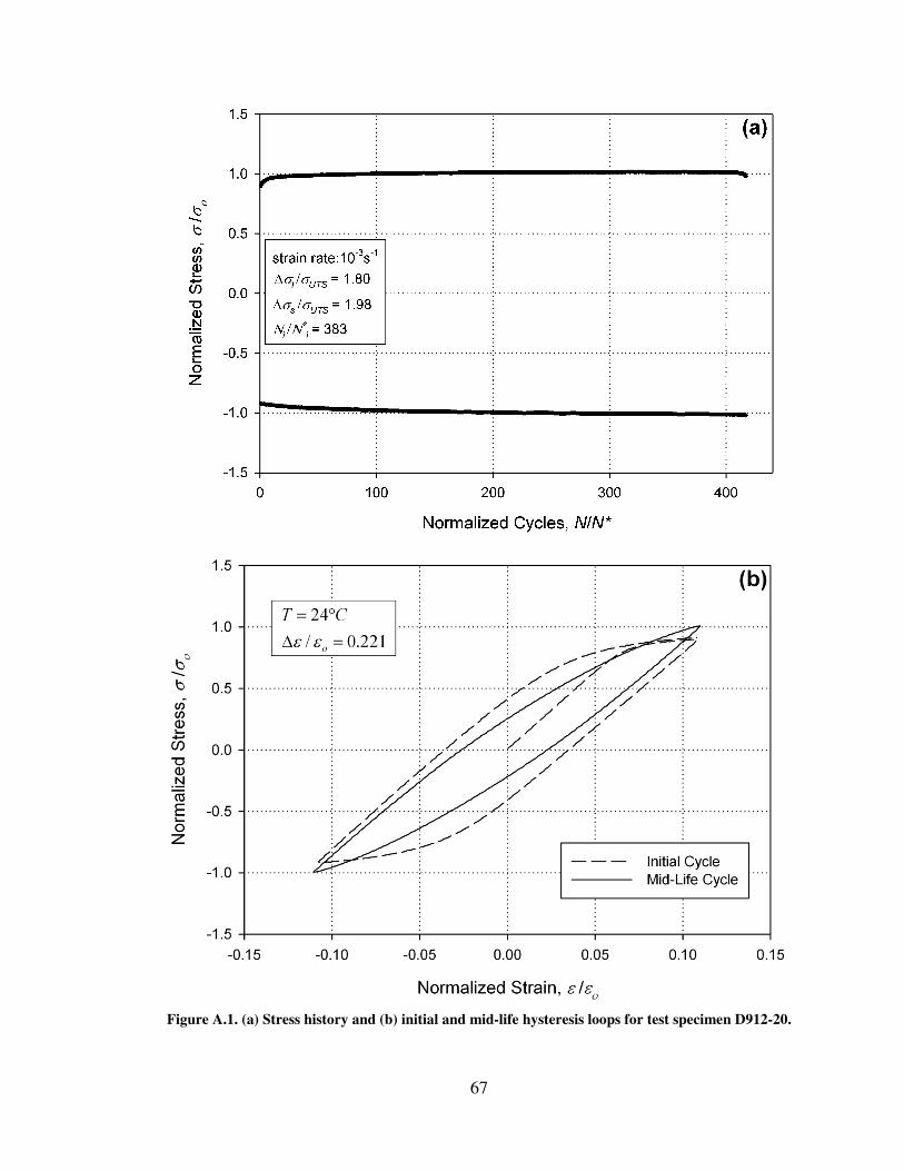
67
Figure A.1. (a) Stress history and (b) initial and mid-life hysteresis loops for test specimen D912-20.
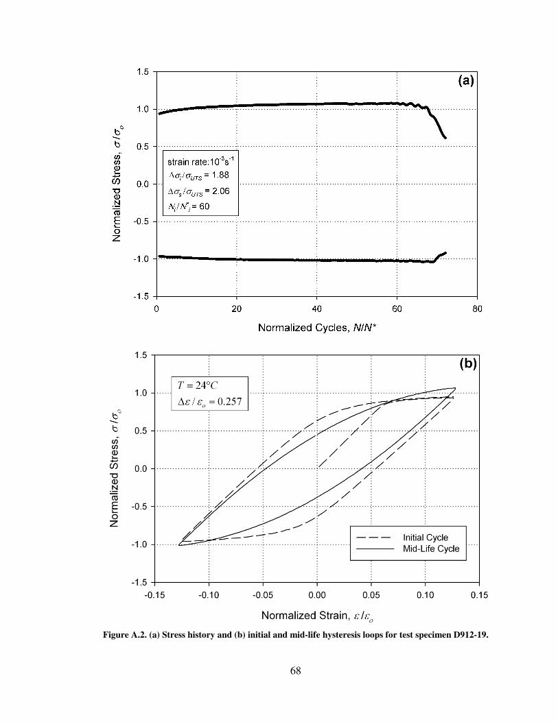
68
Figure A.2. (a) Stress history and (b) initial and mid-life hysteresis loops for test specimen D912-19.
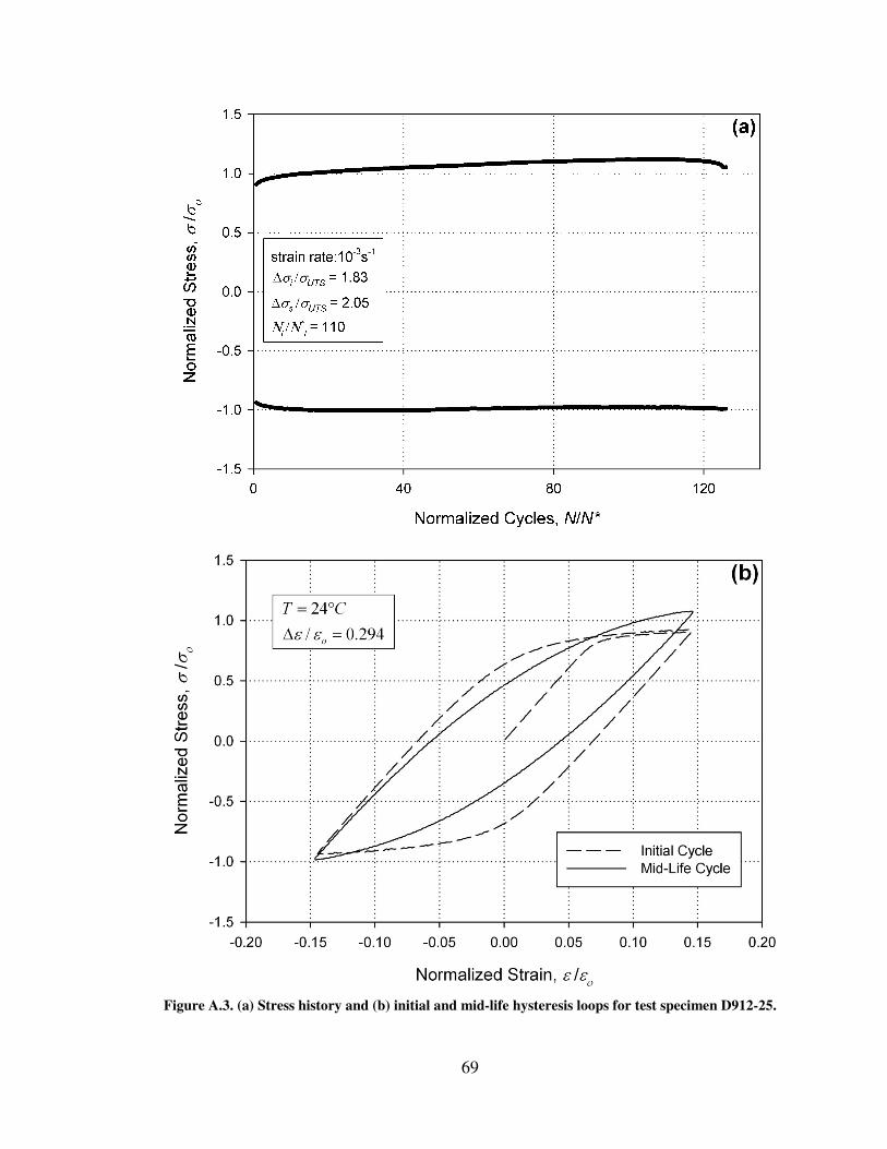
69
Figure A.3. (a) Stress history and (b) initial and mid-life hysteresis loops for test specimen D912-25.
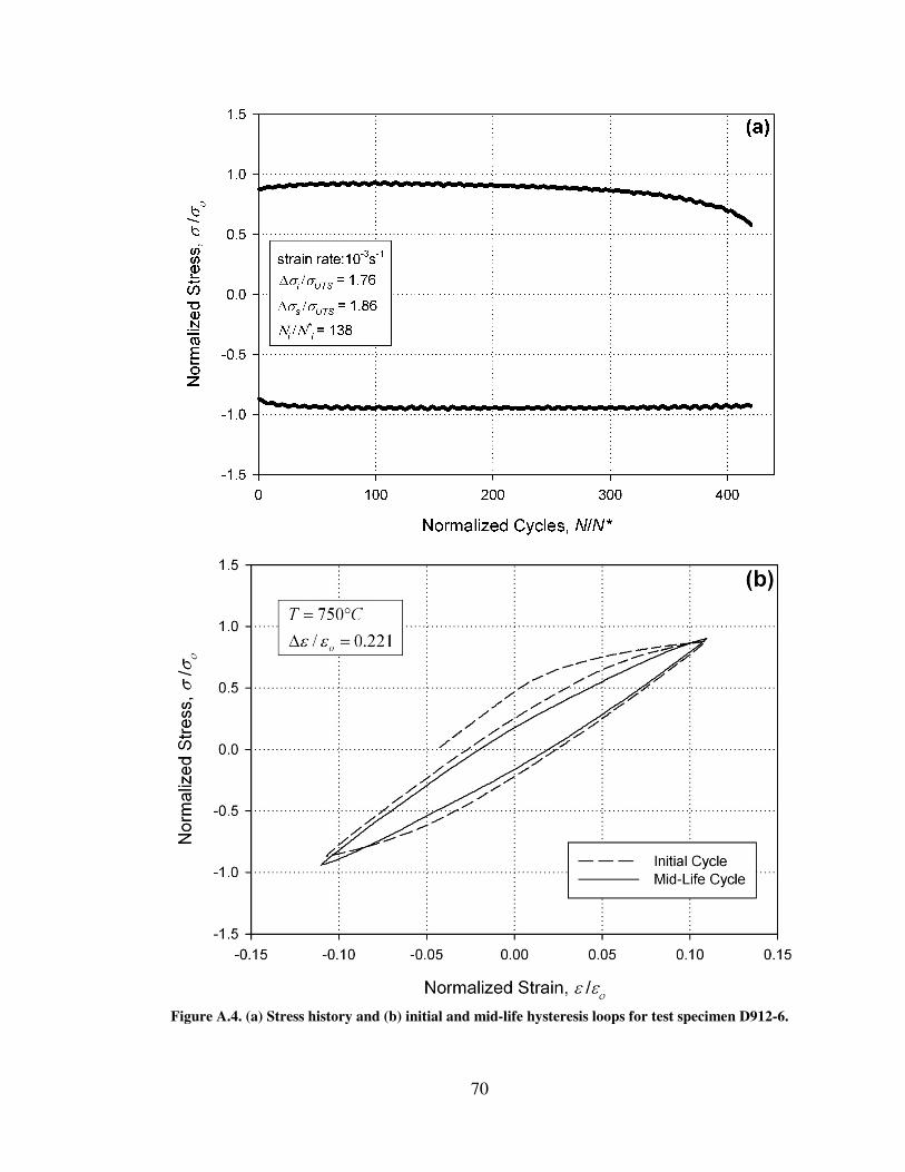
70
Figure A.4. (a) Stress history and (b) initial and mid-life hysteresis loops for test specimen D912-6.
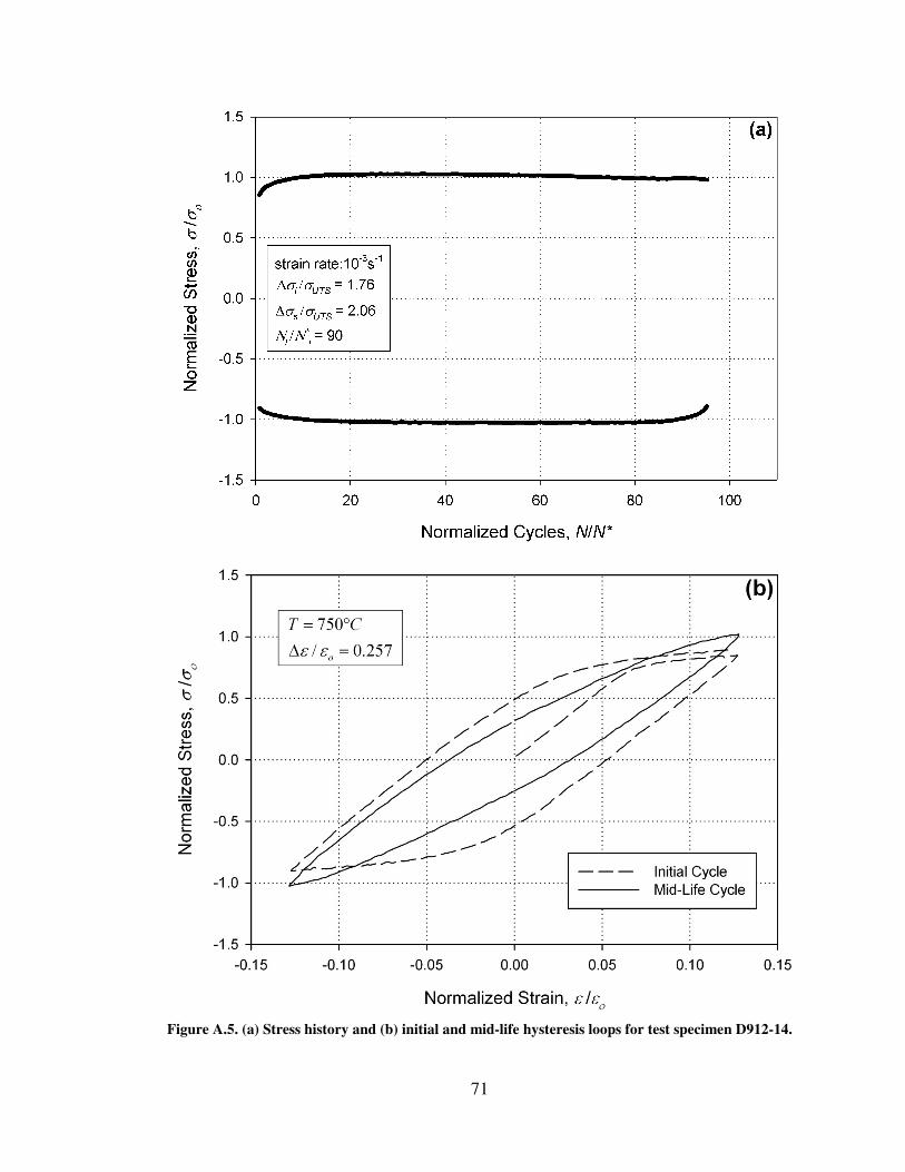
71
Figure A.5. (a) Stress history and (b) initial and mid-life hysteresis loops for test specimen D912-14.
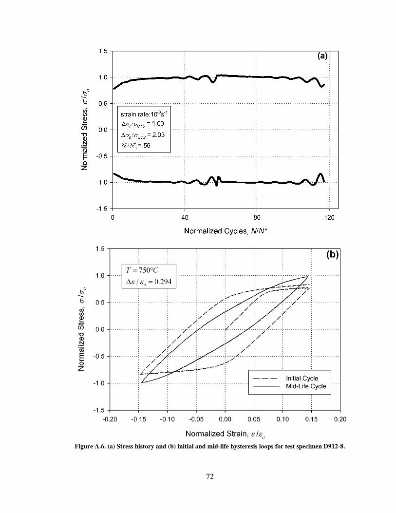
72
Figure A.6. (a) Stress history and (b) initial and mid-life hysteresis loops for test specimen D912-8.
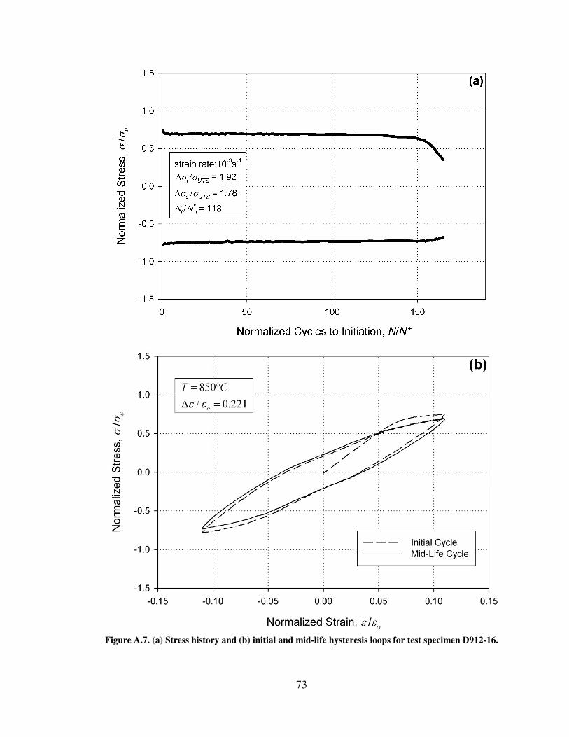
73
Figure A.7. (a) Stress history and (b) initial and mid-life hysteresis loops for test specimen D912-16.
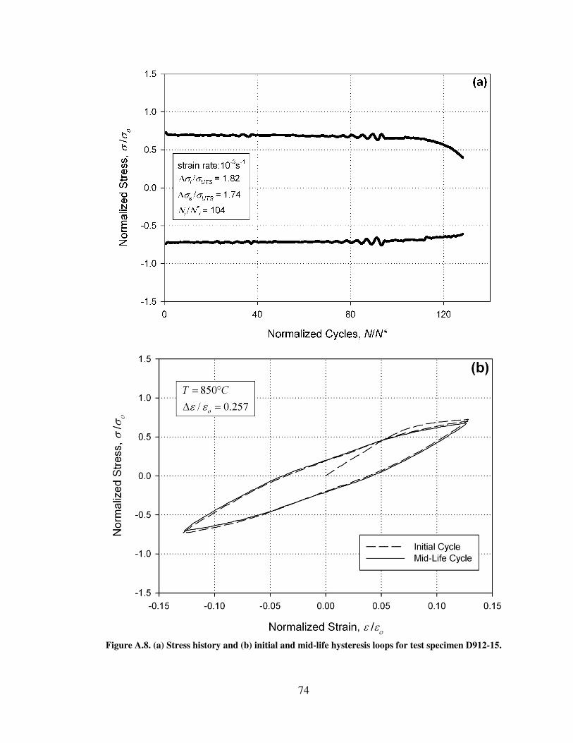
74
Figure A.8. (a) Stress history and (b) initial and mid-life hysteresis loops for test specimen D912-15.
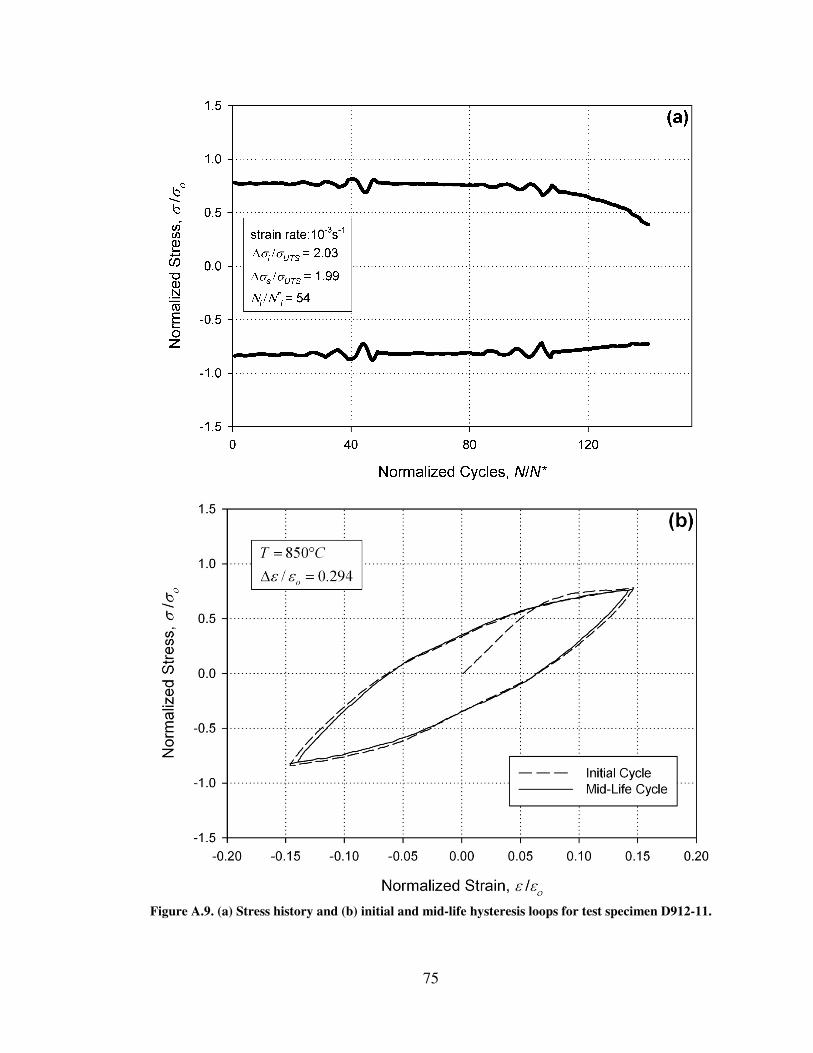
75
Figure A.9. (a) Stress history and (b) initial and mid-life hysteresis loops for test specimen D912-11.
76
APPENDIX B: ITERATIVE DEVELOPMENT OF STRAIN-
LIFE FATIGUE CONSTANTS
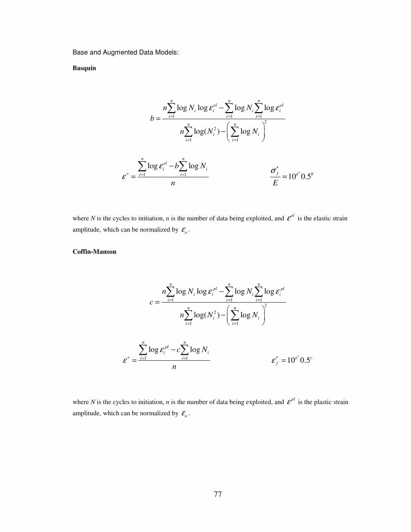
77
Base and Augmented Data Models:
Basquin
1 1 1
2
2
1 1
log log log log
log( ) log
n n nel el
i i i i
i i i
n n
i i
i i
n N N
b
n N N
ε ε= = =
= =
−
=
−
∑ ∑ ∑
∑ ∑
1 1
log logn n
el
i i
i i
b N
n
ε
ε∗ = =
−
=
∑ ∑
10 0.5
f b
E
εσ ∗′
=
where N is the cycles to initiation, n is the number of data being exploited, and el
ε is the elastic strain
amplitude, which can be normalized by o
ε .
Coffin-Manson
1 1 1
2
2
1 1
log log log log
log( ) log
n n npl pl
i i i i
i i i
n n
i i
i i
n N N
c
n N N
ε ε= = =
= =
−
=
−
∑ ∑ ∑
∑ ∑
1 1
log logn n
pl
i i
i i
c N
n
ε
ε∗ = =
−
=
∑ ∑
10 0.5c
f
εε
∗
′ =
where N is the cycles to initiation, n is the number of data being exploited, and pl
ε is the plastic strain
amplitude, which can be normalized by o
ε .
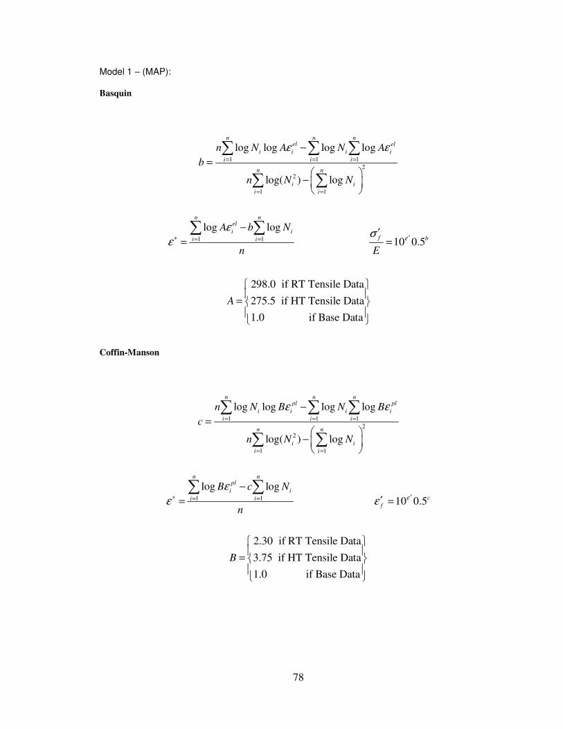
78
Model 1 – (MAP):
Basquin
1 1 1
2
2
1 1
log log log log
log( ) log
n n nel el
i i i i
i i i
n n
i i
i i
n N A N A
b
n N N
ε ε= = =
= =
−
=
−
∑ ∑ ∑
∑ ∑
1 1
log logn n
el
i i
i i
A b N
n
ε
ε∗ = =
−
=
∑ ∑
10 0.5
f b
E
εσ ∗′
=
298.0 if RT Tensile Data
275.5 if HT Tensile Data
1.0 if Base Data
A
=
Coffin-Manson
1 1 1
2
2
1 1
log log log log
log( ) log
n n npl pl
i i i i
i i i
n n
i i
i i
n N B N B
c
n N N
ε ε= = =
= =
−
=
−
∑ ∑ ∑
∑ ∑
1 1
log logn n
pl
i i
i i
B c N
n
ε
ε∗ = =
−
=
∑ ∑
10 0.5c
f
εε
∗
′ =
2.30 if RT Tensile Data
3.75 if HT Tensile Data
1.0 if Base Data
B
=
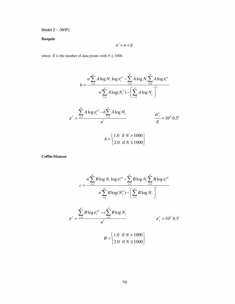
79
Model 2 – (WIP):
Basquin
n n n′ = +
where n is the number of data points with N < 1000.
1 1 1
2
2
1 1
log log log log
log( ) log
n n nel el
i i i i
i i i
n n
i i
i i
n A N A N A
b
n A N A N
ε ε
′ ′ ′
= = =
′ ′
= =
′ −
=
′ −
∑ ∑ ∑
∑ ∑
1 1
log logn n
el
i i
i i
A b A N
n
ε
ε
′ ′
∗ = =
−
=′
∑ ∑
10 0.5
f b
E
εσ ∗′
=
1.0 if 1000
2.0 if 1000
NA
N
> =
≤
Coffin-Manson
1 1 1
2
2
1 1
log log log log
log( ) log
n n npl pl
i i i i
i i i
n n
i i
i i
n B N B N B
c
n B N B N
ε ε
′ ′ ′
= = =
′ ′
= =
′ −
=
′ −
∑ ∑ ∑
∑ ∑
1 1
log logn n
pl
i i
i i
B c B N
n
ε
ε
′ ′
∗ = =
−
=′
∑ ∑
10 0.5c
f
εε
∗
′ =
1.0 if 1000
2.0 if 1000
NB
N
> =
≤
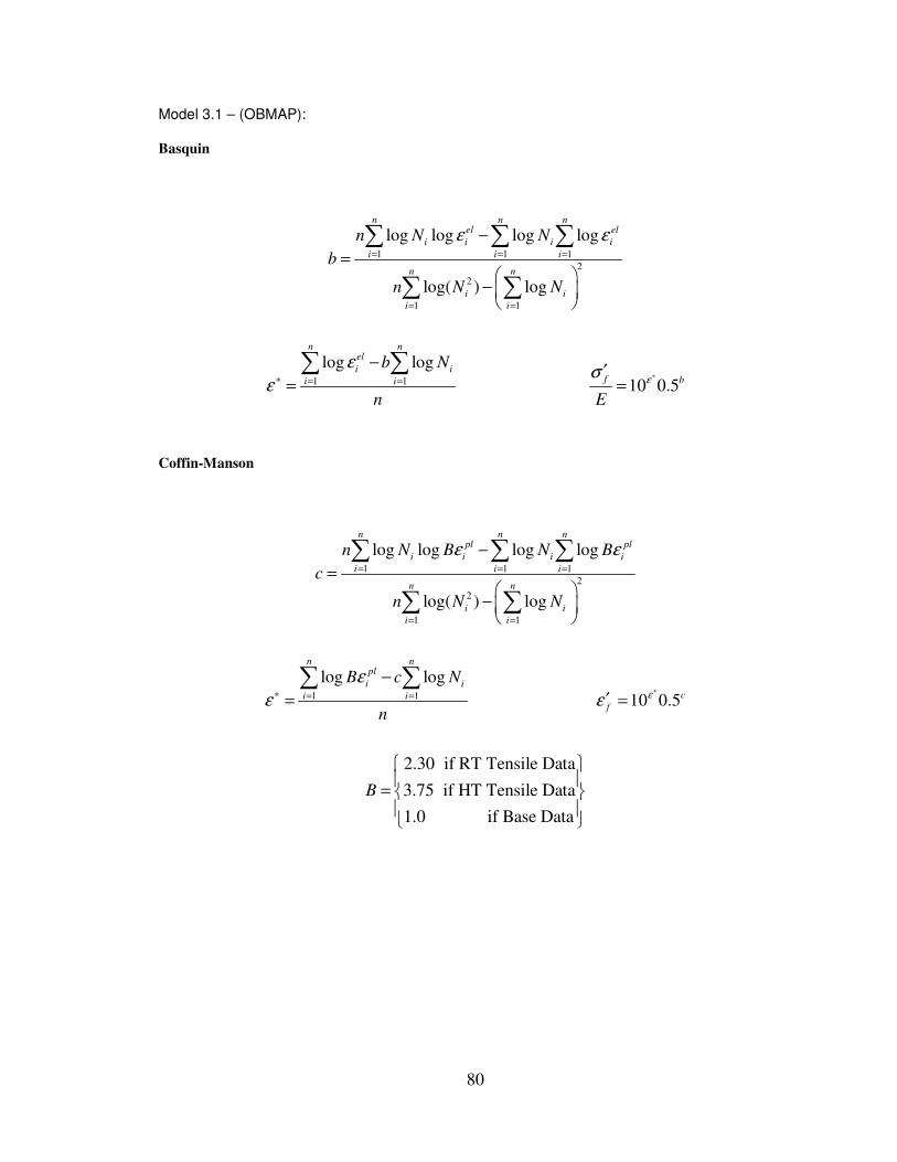
80
Model 3.1 – (OBMAP):
Basquin
1 1 1
2
2
1 1
log log log log
log( ) log
n n nel el
i i i i
i i i
n n
i i
i i
n N N
b
n N N
ε ε= = =
= =
−
=
−
∑ ∑ ∑
∑ ∑
1 1
log logn n
el
i i
i i
b N
n
ε
ε∗ = =
−
=
∑ ∑
10 0.5
f b
E
εσ ∗′
=
Coffin-Manson
1 1 1
2
2
1 1
log log log log
log( ) log
n n npl pl
i i i i
i i i
n n
i i
i i
n N B N B
c
n N N
ε ε= = =
= =
−
=
−
∑ ∑ ∑
∑ ∑
1 1
log logn n
pl
i i
i i
B c N
n
ε
ε∗ = =
−
=
∑ ∑
10 0.5c
f
εε
∗
′ =
2.30 if RT Tensile Data
3.75 if HT Tensile Data
1.0 if Base Data
B
=
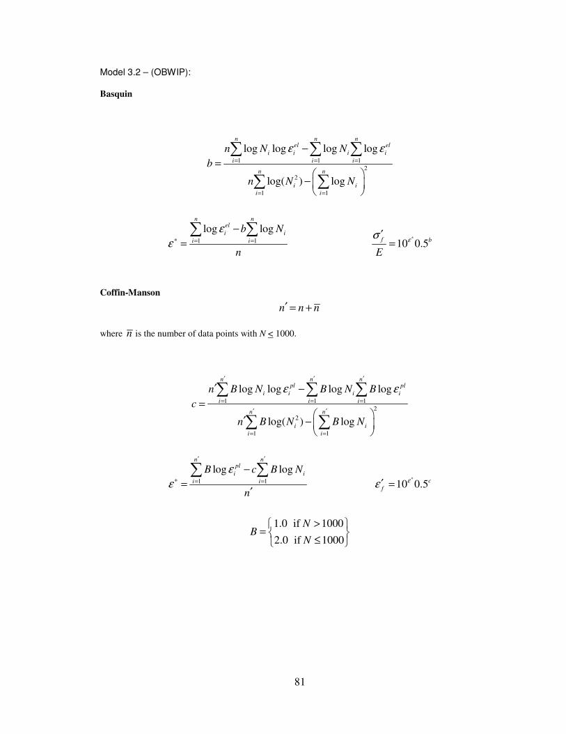
81
Model 3.2 – (OBWIP):
Basquin
1 1 1
2
2
1 1
log log log log
log( ) log
n n nel el
i i i i
i i i
n n
i i
i i
n N N
b
n N N
ε ε= = =
= =
−
=
−
∑ ∑ ∑
∑ ∑
1 1
log logn n
el
i i
i i
b N
n
ε
ε∗ = =
−
=
∑ ∑
10 0.5
f b
E
εσ ∗′
=
Coffin-Manson
n n n′ = +
where n is the number of data points with N < 1000.
1 1 1
2
2
1 1
log log log log
log( ) log
n n npl pl
i i i i
i i i
n n
i i
i i
n B N B N B
c
n B N B N
ε ε
′ ′ ′
= = =
′ ′
= =
′ −
=
′ −
∑ ∑ ∑
∑ ∑
1 1
log logn n
pl
i i
i i
B c B N
n
ε
ε
′ ′
∗ = =
−
=′
∑ ∑
10 0.5c
f
εε
∗
′ =
1.0 if 1000
2.0 if 1000
NB
N
> =
≤
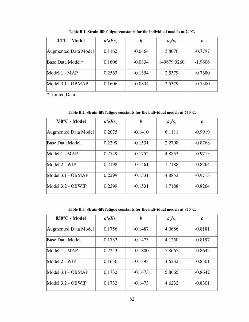
82
Table B.1. Strain-life fatigue constants for the individual models at 24°C.
24°C - Model σ'f/Eεo b ε'f/εo c
Augmented Data Model 0.1162 -0.0464 3.8076 -0.7797
Base Data Model* 0.1606 -0.0834 149679.9260 -1.9606
Model 1 - MAP 0.2563 -0.1354 2.5379 -0.7380
Model 3.1 - OBMAP 0.1606 -0.0834 2.5379 -0.7380
*Limited Data
Table B.2. Strain-life fatigue constants for the individual models at 750°C.
750°C - Model σ'f/Eεo b ε'f/εo c
Augmented Data Model 0.2075 -0.1410 6.1111 -0.9919
Base Data Model 0.2299 -0.1531 2.2708 -0.8768
Model 1 - MAP 0.2749 -0.1752 4.8853 -0.9713
Model 2 - WIP 0.2198 -0.1461 1.7188 -0.8264
Model 3.1 - OBMAP 0.2299 -0.1531 4.8853 -0.9713
Model 3.2 - OBWIP 0.2299 -0.1531 1.7188 -0.8264
Table B.3. Strain-life fatigue constants for the individual models at 850°C.
850°C - Model σ'f/Eεo b ε'f/εo c
Augmented Data Model 0.1756 -0.1487 4.0686 -0.8181
Base Data Model 0.1732 -0.1473 4.1250 -0.8197
Model 1 - MAP 0.2243 -0.1800 5.8665 -0.8642
Model 2 - WIP 0.1636 -0.1393 4.6232 -0.8301
Model 3.1 - OBMAP 0.1732 -0.1473 5.8665 -0.8642
Model 3.2 - OBWIP 0.1732 -0.1473 4.6232 -0.8301
83
REFERENCES
Albeirutty, M.H., Alghamdi, A.S. and Najjar, Y.S. (2004). “Heat Transfer Analysis for a
Multistage Gas Turbine Using Different Blade-Cooling Schemes”, Applied Thermal
Engineering, Vol. 24, pp. 563-577.
Alloy IN738 Technical Data Leaflet. (1985). Nickel Development Institute, Inco Limited
Publication No. 497.
ASTM International E606-04. (2004). “Standard Practice for Strain-Controlled Fatigue
Testing”, West Conshohocken, PA. ASTM International.
ASTM International E739-91. (2004). “Standard Practice for Statistical Analysis of
Linearized Stress-Life (S-N) and Strain-Life (ε-N) Fatigue Data”, West
Conshohocken, PA. ASTM International.
Balikci, E. (1998). “Microstructure Evolution and Its Influence on Thermal Expansion
and Tensile Properties of the Superalloy IN738LC at High Temperatures”, Doctoral
Dissertation, Mechanical Engineering Dept., Louisiana State University, Baton
Rouge, Louisiana.
Bettge, D., Osterle, W. and Ziebs, J. (1995). “Temperature Dependence of Yield Strength
and Elongation of the Nickel-base Superalloy IN 738 LC and the Corresponding
Microstructural Evolution”, Zeitschrift fur Metallkunde, Vol. 86, No. 3, pp. 190-
197.
Brown, W.F. and Setlak, S.J. (2001). Aerospace Structural Metals Handbook, 38th
Edition, Purdue University, West Lafayette, IN.
84
Choe, B.H., Shin, J.K., Shin, S.K., Lee, J.H., Paik, U., Yeom, J.T. and Park, N.K. (2006).
“Estimation of Low Cycle Fatigue Life on the Accumulated Hysteresis Energy of
∆σ ∙ ∆εp for Direct Aged Alloy 718”, Materials Science Forum, Vol. 510, pp. 482-
485.
Danzer, R. and Bressers, J. (1986). “A Method To Predict The Life Under High-
Temperature Low Cycle Fatigue Conditions”, Fatigue and Fracture of Engineering
Materials and Structures, Vol. 9, No. 3, pp. 151-168.
Day, M.F. and Thomas, G.B. (1985). “Analysis of the Low Cycle Fatigue Behaviour of
Two Ni-Cr-Base Alloys”, Fatigue of Engineering Materials and Structures, Vol. 8,
No. 1, pp. 33-48.
Dufailly, J. and Lemaitre, J. (1995). “Modeling Very Low Cycle Fatigue”, International
Journal of Fatigue, Vol. 4, pp. 153-170.
Fischmeister, H.F., Danzer, R. and Buchmayr, B. (1986). “Life Time Prediction Models”,
Proceedings of High temperature alloys for gas turbines conference, Lie’ge,
Belgium, pp. 495-549, October 6-9.
Halford, G.R. and Manson, S.S. (1968). “Application of a Method of Estimating High-
Temperature Low-Cycle Fatigue Behavior of Materials”, Transactions of the ASM,
Vol. 61, No. 1, pp. 94-102.
Hou, N.X., Wen, Z.X., Yu, Q.M. and Yue, Z.F. (2009). “Application of a combined high
and low cycle fatigue life model on life prediction of SC blade”, International
Journal of Fatigue, Vol. 31, pp. 616-619.
85
Hyun, J.S., Song, G.W. and Lee, Y.S. (2006). “Thermo-Mechanical Fatigue of the Nickel
Base Superalloy IN738LC for Gas Turbine Blades”, Key Engineering Materials,
Vol. 321, pp. 509-512.
Itoh, Y., Saitoh, M., Takaki, K. and Fujiyama, K. (2001). “Effect of high-temperature
protective coatings on fatigue lives of nickel-based superalloys”, Fatigue and
Fracture of Engineering Materials and Structures, Vol. 24, No. 12, pp. 843-854.
Jianting, G. and Ranucci, D. (1983). “Low Cycle Fatigue Behaviour of Cast Nickel-Base
Superalloy IN738LC at Room Temperature”, International Journal of Fatigue, Vol.
5, No. 2, pp. 95-97.
Jianting, G., Ranucci, D., Picco, E. and Strocchi, P.M. (1984). “Effect of the
Environment on the Low Cycle Fatigue Behaviour of Cast Nickel-Base Superalloy
IN738LC”, International Journal of Fatigue, Vol. 6, No. 2, pp. 95-99.
Kuroda, M. (2001). “Extremely Low Cycle Fatigue Life Prediction Based on a New
Cumulative Fatigue Damage Model”, International Journal of Fatigue, Vol. 24, pp.
699-703.
Manson, S.S. (1965). “Fatigue: A Complex Subject – Some Simple Approximations”,
Experimental Mechanics, Vol. 5, No. 7, pp. 193-226.
Manson, S.S. (1968). “A Simple Procedure for Estimating High-temperature Low-cycle
Fatigue”, Experimental Mechanics, Vol. 8, No. 8, pp. 349-355.
Marchionni, M., Ranucci, D. and Picco, E. (1982). “High-Temperature Low-Cycle
Fatigue Behaviour of IN738LC Alloy in Air and in Vacuum”, Proceedings of High
temperature alloys for gas turbines conference, Lie’ge, Belgium, pp. 791-804.
October 4-6.
86
Matsuda, N., Umezawa, S. and Terunuma F. (1986). “Small Crack Initiation and Growth
Behavior of IN738LC at Low Cycle Fatigue and Thermal Fatigue”, The Society of
Materials Science, Japan, pp. 100-106.
Mazur, Z., Luna-Ramirez, A., Juarez-Islas, J.A. and Campos-Amezcua, A. (2005).
“Failure Analysis of a Gas Turbine Blade Made of Inconel 738LC Alloy”,
Engineering Failure Analysis, Vol. 12, pp. 474-486.
Meggiolaro, M.A. and Castro, J.T.P. (2004). “Statistical Evaluation of Strain-Life Fatigue
Crack Initiation Predictions”, International Journal of Fatigue, Vol. 26, pp. 463-
476.
Morrow, J. and Tuler, F.R. (1965). “Low Cycle Fatigue Evaluation of Inconel 713C and
Waspaloy”, Transactions of the ASME, Journal of Basic Engineering, Vol. 87, No.
2, pp. 275-289.
Ondera, H., Ro, Y., Yamagata, T. and Yamazaki, M. (1986). “The Effect of Tensile
Strength and Ductility on High-Temperature Low-Cycle Fatigue of Cast Ni-base
Superalloys”, Transactions of the National Research Institute for Metals, Vol. 28,
No. 2, pp. 112-120.
Ong, J.H. (1993). “An improved technique for the prediction of axial fatigue life from
tensile data”, International Journal of Fatigue, Vol. 15, No. 3, pp. 213-219.
Park, J.H. and Song, J.H. (1995). “Detailed Evaluation of Methods for Estimation of
Fatigue Properties”, International Journal of Fatigue, Vol. 17, No. 5, pp. 365-373.
Persson, C., Burman, G. and Lindblom, Y. (1986). “Behavior of Nimonic 105 and
IN738LC Under Creep and LCF Testing”, Proceedings of High temperature alloys
for gas turbines conference, Lie’ge, Belgium, pp. 1501-1515. October 6-9.
87
Petrenec, M., Obrtlik, J. and Polak, J. (2007). “High Temperature Low Cycle Fatigue of
Superalloys Inconel 713LC and Inconel 792-5A”, Key Engineering Materials, Vol.
348, pp. 101-104.
Radonovich, D.C. (2007). “Methods of Extrapolating Low Cycle Fatigue Data to High
Stress Amplitudes”, Master’s Thesis, Dept. of Mechanical, Materials and Aerospace
Engineering, University of Central Florida, Orlando, Florida.
Radonovich, D.C. and Gordon, A. P. (2008). “Methods of Extrapolating Low Cycle
Fatigue Data To High Stress Amplitudes”, Proceedings of ASME Turbo Expo:
Power for Land, Sea, and Air, Berlin, Germany, pp. 1-10. June 9-13.
Scarlin, R.B. (1975). “Fatigue Crack Growth in a Cast Ni-Base Alloy”, Material Science
and Engineering, Vol. 21, No. 2, pp. 139-147.
Tateishi, K., Hanji, T. and Minami, K. (2007). “A Prediction Model for Extremely Low
Cycle Fatigue Strength of Structural Steel”, International Journal of Fatigue, Vol.
29, pp. 887-896.
Troshchenko V.T., Gryaznov, B.A., Malashenko, I.S., Nalimov, Y.S. and Rabinovich
A.A. (2007). “Cyclic Strength of Turbine Blades Made of Cast Nickel-Base
Alloys”, Strength of Materials, Vol. 39, No. 2, pp. 109-115.
Wu, X., Beres, W. and Yandt, S. (2008). “Challenges in Life Prediction of Gas Turbine
Critical Components”, Canadian Aeronautics and Space Journal, Vol. 54, No. 2,
pp. 31-39.
Xue, L. (2008). “A Unified Expression for Low Cycle Fatigue and Extremely Low Cycle
Fatigue and Its Implication for Monotonic Loading”, International Journal of
Fatigue, Vol. 30, pp. 1691-1698.
Recommended