Export Variety and Country Productivity: ESTIMATING THE MONOPOLISTIC COMPETITION
MODEL WITH ENDOGENOUS PRODUCTIVITY
by
Robert Feenstra Department of Economics
University of California, Davis and NBER
Hiau Looi Kee
The World Bank
July 2007
Abstract
This paper provides evidence on the monopolistic competition model with heterogeneous firms and endogenous productivity. We show that this model has a well-defined GDP function where relative export variety enters positively, and estimate this function over 48 countries from 1980 to 2000. Average export variety to the United States increases by 3.3% per year, so it nearly doubles over these two decades. The total increase in export variety is associated with a 3.3% average productivity improvement for exporters over the two decades. Overall, the model can explain 31% of the within-country variation in productivity (or 52% for the OECD countries), but only a very small fraction of the between-country variation in productivity. JEL code: F12, F14 Keywords: productivity, export variety, translog, monopolistic competition * The authors thank Russell Davidson, Jonathan Eaton, Marcelo Olarreaga, David Weinstein and the anonymous referees for helpful comments. Research funding from the World Bank is cordially acknowledge. The findings, interpretations, and conclusions expressed in this paper are entirely those of the authors, and do not necessarily represent the view of the World Bank, its Executive Directors, or the countries they represent. Address for contact: Robert Feenstra, Department of Economics, University of California, Davis, CA 95616; Phone (530)752-7022; Fax,(530)752-9382; E-mail, [email protected].
1. Introduction
Empirical research in international trade (as well as other fields) has made it clear that
productivity levels differ a great deal across countries.1 This conclusion begs the question of
where the technology differences come from. While various explanations have been proposed
that do not depend on international trade,2 our interest here is whether trade itself can explain the
productivity differences across countries. This conclusion is suggested by recent models of
monopolistic competition and trade in which productivity levels are endogenous.
Two examples of this recent literature are Eaton and Kortum (2002) and Melitz (2003).
Eaton and Kortum allow for stochastic differences in technologies across countries, with the
lowest cost country becoming the exporter of a product variety to each location. In that case, the
technologies utilized in a country will depend on its distance and trade barriers with other
countries. Melitz allows for stochastic draws of technology for each firm, and only those firms
with productivities above a certain cutoff level will operate. A subset of these firms – the most
productive – also become exporters. Melitz shows how the average productivity in a country is
affected by changes in trade barriers and transport costs. A reduction in trade barriers, for
example, pushes the less efficient firms to exit the market while draws more firms into exporting.
It follows that average country productivity rises.
Empirical testing of this class of models can proceed by utilizing firm-level data and
inferring the productivity levels of firms. That approach is taken by Bernard et al (2003) for U.S.
firms; Eaton, Kortum and Kramarz (2003, 2004) for French firms; Helpman, Melitz and Yeaple
(2004) for U.S. multinationals operating abroad; and Demidova, Kee and Kala (2006) for
Bangladeshi garment exporters. When firm level data are available, it is highly desirable to make 1 See, for example, the work of Trefler (1993, 1995), and Davis and Weinstein (2001). 2 Explanations for the aggregate productivity differences across countries include geography/climate (Sachs, 2001), colonial institutions (Acemoglu, et al, 2001), or social capital (Jones and Hall, 1999).
2
use of it like these authors do. But for many countries such data are not available, and in those
cases, we are still interested in determining the extent to which openness to trade can explain
country productivity. That is our objective in this paper, using a broad cross-section of advanced
and developing nations and disaggregating across sectors.
In section 2 we review the monopolistic competition model with heterogeneous firms,
from Melitz (2003), Bernard, Redding and Schott (2004) and Chaney (2005). We emphasize
some features of that model that these authors do not: for example, the “cutoff” productivity of
firms producing for either the domestic or export markets are both at the socially optimal level.
This means that we can use a GDP function for the economy, similar to the competitive case. In
each sector, only a subset of firms become exporters, and these are the most productive firms. It
follows that when the share of exporting firms rises, or equivalently, the share of exported
varieties rises, then average productivity and GDP increase. Therefore, relative export variety is
positively related to GDP.3
Our empirical specification is developed in section 3. We draw on Harrigan (1997), who
estimates a translog GDP function in a competitive model allowing for industry productivity
differences across countries. In our case, the export variety of each industry enters the GDP
function instead. A goal of the empirical work is to determine what amount of the productivity
differences across countries and over time are determined by variation in export variety, which is
treated as an endogenous variable. The instrumental variables used to determine export variety
are those suggested by our model: tariffs, trade agreements and distance. The index of export
variety we use draws on Feenstra (1994), and has been employed recently by Hummels and
Klenow (2005) and Broda and Weinstein (2006). Using this measure, average export variety to
3 With a Pareto distribution for firm productivities, we also show that relative export variety enters with an exponent related to the elasticity of substitution and the Pareto productivity parameter. This result is similar to the formulation of the gravity equation in Chaney (2005).
3
the U.S. has increased by 3.3% per year over 1980-2000, so export variety nearly doubles over
the two decades.
In section 4 we estimate the GDP function using data on 44 countries from 1980 to 2000,
distinguishing the sectoral outputs of seven sectors. Parameter estimates of the GDP function
show that expansion of export variety over 1980-2000 explains a 3.3% increase in exporters’
productivity. Since average export variety also grew 3.3% per year, a rule of thumb is that a x%
per annum sustained growth in export variety over two decades leads to an overall productivity
improvement for the exporter of x%. This is an estimate of the endogenous portion of
productivity gains. In the time series, export variety explains 31.1% of within-country variation
in productivity, and 52.2% for just the OECD countries. But this linkage between export variety
and productivity is not enough to explain the enormous cross-country differences in productivity.
Allowing for country fixed effects, export variety explains only 0.3% of the between-country
variation in productivity, or 3.3% for the OECD countries. We conclude that export variety in the
monopolistic competition model with heterogeneous firms is quite effective at accounting for the
time-series variation in productivity within countries, but cannot explain the large absolute
differences in productivity between them.
2. Monopolistic Competition with Heterogeneous Firms
We assume some familiarity with the monopolistic competition model of Melitz (2003),
and outline here a two-country, multi-factor, multi-sector version that also draws upon Bernard,
Redding and Schott (2005) and Chaney (2005). We focus on the home country H, while denoting
foreign variables with the superscript F.
In each sector i = 1,…,N at home, there is a mass of Mi firms operating in equilibrium.
Each period, a fraction δ of these firms go bankrupt and are replaced by new entrants. Each new
4
entrant pays a fixed cost to receive a draw iϕ of productivity from a cumulative distribution
),(G ii ϕ which gives rise to the marginal cost of ii /m ϕ . Only those firms with productivity
above a cutoff level *iϕ find it profitable to actually produce (the cutoff level will be determined
below). Letting Mie denote the mass of new entrants in sector i, then ie*ii M)](G1[ ϕ− firms
successfully produce. In a stationary equilibrium, these should replace the firms going bankrupt,
so that: iie
*ii MM)](G1[ δ=ϕ− . (1)
Conditional on successful entry, the distribution of productivities for firms in sector i is then:
⎪⎪⎩
⎪⎪⎨
⎧ ϕ≥ϕϕ−
ϕ
=ϕμ
,otherwise0
,if)](G1[
)(g
)(
*ii*
ii
ii
ii (2)
where iiiii /)(G)(g ϕ∂ϕ∂=ϕ .
Home and foreign consumers both have CES preferences that are symmetric over product
varieties. Given home expenditure of HiE in sector i, it follows that the revenue earned by a
home firm from selling in the domestic sector i at the price )(p ii ϕ is:
Hi
1
Hi
iiiiiiii E
P)(p)(q)(p)(r
iσ−
⎥⎥⎦
⎤
⎢⎢⎣
⎡ ϕ=ϕϕ=ϕ , σi > 1, (3)
where )(q ii ϕ is the quantity sold and HiP is the home CES price index for sector i:
ii
*Fix
i
*i
11
iiFi
Fi
1i
Fiiiii
1ii
Hi d)(M)(pd)(M)(pP
σ−σ−
∞
ϕ
σ−∞
ϕ ⎥⎥⎦
⎤
⎢⎢⎣
⎡ϕϕμϕ+ϕϕμϕ= ∫∫ . (4)
The first integral in this expression is taken over home firms, with prices )(p ii ϕ and mass Mi,
5
selling in the domestic market. The second integral is taken over foreign firms, with prices
)(p iFi ϕ and mass F
iM , exporting to the home market.
In our analysis below it will be convenient to treat revenue as a function of quantity.
Using the second equality in (3) to solve for price as a function of quantity, and substituting this
back into (3), we obtain:
i
i 1
iiidii )(qA)(r σ−σ
ϕ=ϕ , where i
1
Hi
HiH
iid PEPA
σ
⎟⎟⎠
⎞⎜⎜⎝
⎛≡ . (3')
We introduce the notation Aid as shift parameter in the demand curve facing home firms for their
domestic sales. It depends on the CES price index HiP , and also on domestic expenditure H
iE in
sector i. Home firms takes both these as given when maximizing profits.
While firms with productivities *ii ϕ≥ϕ find it profitable to produce for the domestic
market, those with productivities *i
*ixi ϕ≥ϕ≥ϕ find it profitable to export. A home firm
exporting in sector i faces the iceberg transport costs of 1i ≥τ meaning that τi units must be sent
in order for one unit to arrive in the foreign country. Letting )(p iix ϕ and )(q iix ϕ denote the
price received and quantity shipped at the factory-gate, 4 the revenue earned by the exporter is:
Fi
1
Fi
iiixiixiixiix E
P)(p)(q)(p)(r
iσ−
⎥⎥⎦
⎤
⎢⎢⎣
⎡ τϕ=ϕϕ=ϕ , (5)
where FiP is the aggregate CES price for sector i in the foreign country, and F
iE is foreign
expenditure in sector i. Once again, it is convenient to treat revenue as a function of quantity,
4 Notice that we are measuring export price and quantity at the factory-gate, or f.o.b., net of any transport costs. The c.i.f. prices would instead be τipix, and the quantity inclusive of the amount lost in transit would be qix/τi. It would be equivalent to use these c.i.f. prices and quantities, but we find it convenient to use the f.o.b. variables since they show how the transport costs τi enter the export shift parameter in (5').
6
which is determined from (5) as:
i
i 1
iixixiix )(qA)(r σ−σ
ϕ=ϕ , where i
1
Fi
Fii
i
Fi
ix PEPA
σ
⎟⎟⎠
⎞⎜⎜⎝
⎛ τ⎟⎟⎠
⎞⎜⎜⎝
⎛
τ≡ . (5')
We introduce the notation Aix as shift parameter in the demand curve facing home firms for their
export sales. It depends on the foreign CES price index FiP , foreign expenditure F
iE , and the
transport costs in sector i.
Integrating (3') and (5'), we obtain revenue from domestic and export sales in sector i:
iii
1
iiidiid d)()(qAMR i
i
*i
ϕϕμϕ≡ σ−σ∞
ϕ∫ , (6)
iii
1
iixixiix d)()(qAMR i
i
*ix
ϕϕμϕ≡ σ−σ∞
ϕ∫ . (7)
Notice that the mass of domestic firms or varieties is ∫∞
ϕ=ϕϕμ*
iiiiii Md)(M , which we are
aggregating over in (6). But the mass of exporting firms or varieties that we are aggregating over
in (7) is iiiiiix Md)(MM *ix
≤ϕϕμ≡ ∫∞
ϕ. It will be convenient to denote the range of export
varieties relative to domestic varieties by:
1)(G1)(G1d)(
MM
*i
*ix
ii
ixi
*ix
≤⎟⎟⎠
⎞⎜⎜⎝
⎛
ϕ−
ϕ−=
⎟⎟⎟
⎠
⎞
⎜⎜⎜
⎝
⎛ϕϕμ=⎟⎟
⎠
⎞⎜⎜⎝
⎛≡χ ∫
∞
ϕ
. (8)
On the resource side, firms producing for the domestic market have fixed costs of fi, and firms
who are exporters have the added fixed cost of fix. We allow for multiple factors of production,
and assume that these fixed costs use the resources in the same proportion as do variable costs in
each sector. The resource constraints for the economy as detailed in the Appendix. Total GDP in
the economy is obtained by summing revenue over the sectors:
7
ixN
1i id RRR += ∑ =. (9)
Consider now a social planner’s problem of maximizing GDP in (9), subject to the
resource constraints for the economy. In maximizing GDP we will hold fixed the shift
parameters Aid and Aix , i = 1,…,N, which is analogous to holding product prices constant in a
conventional GDP function. Then we show in the Appendix that:
Proposition 1
Choose )(q ii ϕ , )(q iix ϕ , ,*iϕ ,*
ixϕ and Mi for i = 1,…,N, to maximize GDP in (9), subject to the
resource constraints for the economy. Holding fixed the shift parameters )A,...,A(A Ndd1d =
and )A,...,A(A Nxx1x = , the first-order conditions for an interior maximum are identical to the
equilibrium conditions for the monopolistically competitive economy. Then GDP can be written
as a function )V,A,A(R xd , which is homogeneous of degree one in )A,A( xd and in V.
The proof of Proposition 1 proceeds by setting up the Lagrangian and obtaining the first-
order conditions. Details are provided in the Appendix, and here we simply describe the results.
The first-order conditions to maximize GDP specify that marginal revenue equal marginal cost in
each sector for both the domestic and export market:
i
iii
i
i c)(p1ϕ
=ϕ⎟⎟⎠
⎞⎜⎜⎝
⎛σ−σ , and
i
iiix
i
i c)(p1ϕ
=ϕ⎟⎟⎠
⎞⎜⎜⎝
⎛σ−σ , (10)
where ci represents marginal costs. Using (10), we can calculate profits from domestic and
export sales as iiiiiiiii /)(r)(q)/c()(r σϕ=ϕϕ−ϕ , and iiixiixiiiix /)(r)(q)/c()(r σϕ=ϕϕ−ϕ .
In addition, the first-order condition specify that the productivity cutoffs *iϕ and *
ixϕ are:
iii*ii fc/)(r =σϕ , and ixii
*ixix fc/)(r =σϕ , (11)
8
which are the zero-cutoff-profit conditions of Melitz (2003).5
Proposition 1 shows that the optimal choices for quantities and cutoff-productivities by
individual firms are identical to the constrained social optimum, where we hold constant the shift
parameters in demand.6 As discussed more fully in the Appendix, this GDP function satisfies
similar properties as in the competitive case, but estimating this function will be more difficult
than in the competitive case for several reasons. First, the shift parameters are endogenous, since
they depend on the country price indexes in (3') and (5') which are endogenous. Second, the shift
parameters are not directly observed, so we will need to develop some proxies for them. Third,
we still need to determine the appropriate functional form for the GDP function. We address
these issues in the next section, using a Pareto distribution for firm productivities.
2.2 Functional Form for GDP
Following Helpman, Melitz and Yeaple (2004) and Chaney (2005), we assume the Pareto
distribution for productivities, defined by:
iiii 1)(G θ−ϕ−=ϕ , with 1ii −σ>θ . (12)
The parameter iθ is a measure of dispersion of the Pareto distribution, with lower iθ having
more weight in the upper tail. Using this distribution, we calculate export relative to domestic
variety in (8) as:
5 Fixed costs are multiplied by ci in (11) because we use the same factor proportions in fixed and marginal costs. 6 Helpman and Krugman (1985, p. 139) also derive a GDP function for a two-sector economy with monopolistic competition (and symmetric costs) in one sector. Because of the constraint we have used that the shift parameters are hold constant, we cannot necessarily interpret our solution as an unconstrained social optimum. Nevertheless, Dixit and Stiglitz (1977) argue that by adding the constraint that firms do not earn negative profits in autarky, then the equilibrium of the symmetric monopolistic competition model is also the constrained first-best for consumers. Further, once we add international trade, then the constraint that the export shift parameter is constant can be interpreted as a “small country” assumption: there are many varieties in the world, so that the additional varieties of this country have a negligible effect on the world price index.
9
i
*ix
*i
*i
*ix
i)(G1)(G1
θ
⎟⎟⎠
⎞⎜⎜⎝
⎛
ϕ
ϕ=⎟
⎟⎠
⎞⎜⎜⎝
⎛
ϕ−
ϕ−=χ . (13)
Relative export variety can be further simplified by using (3) and (5) to compute )(r *ii ϕ
and )(r *ixix ϕ , together with the equilibrium conditions (10) and (11). Then we obtain:
i
ixHi
Fi
1
Hi
*i
iFi
*ix
*ii
*ixix
ff
EE
P/P
)(r)(r i
=⎟⎟⎠
⎞⎜⎜⎝
⎛
ϕ
τϕ=
ϕ
ϕ−σ
.
Raising this expression to the power (1/σi), and re-arranging, we have:
i
ii
i /1
i
ix1
iid
ixff
AA σ
θσ−σ
⎟⎟⎠
⎞⎜⎜⎝
⎛χ=
⎟⎟
⎠
⎞
⎜⎜
⎝
⎛, 110
ii
i <θσ−σ
< . (14)
Thus, the ratio of the export/domestic shift parameters in demand equals relative export variety
raised to a positive power, adjusted for a term involving fixed costs. This means that relative
export variety can be used as a proxy for (Aix/Aid).
The Pareto distribution further enables us to aggregate domestic and export sales in each
sector. In particular, we shown in the Appendix that the Pareto distribution, along with condition
(11), allows us to write export sales relative to domestic sales in each sector as:
⎟⎟⎠
⎞⎜⎜⎝
⎛χ=
i
ixi
id
ixff
RR . (15)
As one might expect, relative export variety is directly related to relative export sales. Then
substituting from (14), the ratio of export to domestic sales becomes:
)1(1
i
ix)1(
id
ix
id
ix i
i
i
ii
ff
AA
RR −σ
θ−
−σθσ
⎟⎟⎠
⎞⎜⎜⎝
⎛⎟⎟⎠
⎞⎜⎜⎝
⎛= . (16)
10
Thus, the sales ratio is a constant-elasticity function of the relative export shift parameters. This
implies that: first, the shift parameters (Aix, Aid) for sector i are weakly separable from all other
variables in the GDP function; and second, the appropriate aggregator for (Aix, Aid) is a CES
function. These results are summarized by:
Proposition 2
Assume that the distribution of firm productivity in Pareto, as in (12). Then the domestic and
export shift parameters (Aid, Aix) can be aggregated into a CES function:
ii
i
i
i
i
ii
i
ii
)1(
)1(1
iix)1(
ix)1(
idixidi )f/f(AA)A,A(θσ−σ
−σθ
−−σθσ
−σθσ
⎥⎥⎥
⎦
⎤
⎢⎢⎢
⎣
⎡+≡ψ . (17)
GDP can be written as a function )V,,...,(R N1 ψψ , and if R is differentiable then:
R)RR(
lnRln ixid
i
+=
ψ∂∂ , (18)
which is the share of sector i in GDP.
Our finding that the Pareto distribution leads to a CES function between domestic and
exported varieties is related to the results in Chaney (2005), who derives a gravity equation for
country exports to different destination markets. For the case of a single export market, we
can obtain his results by substituting for Aid and Aix from (3') and (5') into (16), obtaining:
⎟⎟⎠
⎞⎜⎜⎝
⎛χ=
i
ixi
id
ixff
RR )1(
1
i
ix)1(
Hi
Fi
Hi
iFi i
i
i
ii
ff
EE
P/P −σ
θ−
−σθ
θ
⎟⎟⎠
⎞⎜⎜⎝
⎛⎟⎟⎠
⎞⎜⎜⎝
⎛⎟⎟⎠
⎞⎜⎜⎝
⎛ τ= . (19)
Thus, the export/domestic share is negatively related to the transport costs, with an exponent of
iθ− in (19), just as in the gravity equation derived by Chaney. The fixed costs in (19) also have
11
the same exponent as found by Chaney (2005). The gravity equation in (19) gives us some
instruments that we can use to explain relative export variety, namely: country size, as measured
by factor endowments, and transport costs, as measured by distance and tariffs.
3. Empirical Specification 3.1 Translog GDP Function
Following Harrigan (1997) we assume a translog functional form for GDP across sectors,
and then use the CES function in (18) within each sector. Introducing the country superscript
h=1,…,H and time subscript t, let )A,A( hixt
hidti
hit ψ=ψ denote the value of that CES function.
Define the vector ),,...,( ht,1N
hNt
ht1
ht +ψψψ=ψ to also include a price h
t,1N+ψ for the non-traded
sector N+1. Denoting factor endowments by the vector )v,...,v(V hKt
ht1
ht = , the translog GDP
function is:
( )
.vlnlnvlnvln
lnlnvlnlnV,Rln
1N
1i
K
1k
hkt
hitik
K
1k
K
1
ht
hktk2
1
1N
1i
1N
1j
hjt
hitij2
1K
1k
hktk
1N
1i
hitit0
h0
ht
ht
ht
∑∑∑∑
∑∑∑∑+
= == =
+
=
+
==
+
=
ψφ+δ+
ψψγ+β+ψα+β+α=ψ
lll
(20)
We allow this function to differ across countries based on the fixed-effects h0α , which reflect
exogenous technology differences, and also allow for the year fixed-effects t0β , which are equal
across countries. In treating all other parameters of the translog function as common across both
countries and time, we are assuming that the distribution function )(G ii ϕ and the fixed costs fi
and fix do not vary over these dimensions.
To satisfy homogeneity of degree one in prices and endowments, we test the restrictions:
12
.0,1,,K
1kik
K
1kk
1N
1iik
1N
1iij
K
1kk
1N
1inkkjiij =φ=δ=φ=γ=β=αδ=δγ=γ ∑∑∑∑∑∑
==
+
=
+
==
+
=lll (21)
As stated in Proposition 2, the share of sector i in GDP equals the derivative of )V,(Rln ht
ht
ht ψ
with respect to hitlnψ :
.1N,...,1i,vlnlnsK
1k
hktik
1N
1j
hjtiji
hit +=φ+ψγ+α= ∑∑
=
+
= (22)
Also, the share of factor k in GDP equals the derivative of )V,(Rln ht
ht
ht ψ with respect to c
ktvln :
.K,...,1k,Plnvlns1N
1i
hitik
K
1
htkk
hkt =φ+δ+β= ∑∑
+
==lll (23)
3.2 CES Sectoral Aggregates
Key to the empirical work is to measure the CES aggregates )A,A( hixt
hidti
hit ψ=ψ in each
sector. To this end, we will difference the GDP and share equations with respect to a comparison
country denoted by F. The CES aggregate in each sector will also be differenced with respect to
country F in log form, which means we take the log of the ratio Fit
hit /ψψ . To evaluate the ratio of
CES functions, we can apply the index number formula due to Sato (1976) and Vartia (1976).
Assuming that the fixed costs fix and fi appearing in (17) are the same across countries, the CES
ratio in sector i equals:
hit
ii
ihit
hit
hit W
)1(
Fit
hit
Fidt
hidt
W
Fidt
hixt
Fidt
hixt
Fidt
hidt
W
Fixt
hixt
W1
Fidt
hidt
Fixt
Fidti
hixt
hidti
AA
A/AA/A
AA
AA
AA
)A,A()A,A( θσ
−σ−
⎟⎟⎠
⎞⎜⎜⎝
⎛
χχ
=⎟⎟⎠
⎞⎜⎜⎝
⎛⎟⎟⎠
⎞⎜⎜⎝
⎛=⎟⎟
⎠
⎞⎜⎜⎝
⎛⎟⎟⎠
⎞⎜⎜⎝
⎛=
ψψ
(24)
where hitW is the logarithmic mean of the export shares in countries h and F.7
7 Let h
itS denote export/(export + domestic) sales in sector i and country h. Then hitW is constructed as:
)]}FitS1ln()h
itS1[ln()]FitS1()h
itS1[()]FitSlnh
itS(ln)FitSh
itS{[()]FitSlnh
itS(ln)FitSh
itS[( //// −−−−−−+−−−− .
13
The first equality in (24) follows directly from the Sato-Vartia formula, which allows us
to evaluate the ratio of CES functions without knowledge of the fixed costs (fix/fi ), but using the
data on export shares instead. The second equality follows by algebra; and the third equality
follows by using (14) to replace the export/domestic shift parameters with relative export variety.
The decomposition in (24) is as far as the theory can take us, and to measure this formula,
we rely on two assumptions. First, we have no data to measure the domestic shift parameters
hidtA in each sector appearing in (24), and will assume that they reflect country-level prices h
tP
plus a sectoral error term:
hit1F
t
ht
Fidt
hidt u
PP
lnAA
ln +⎟⎟⎠
⎞⎜⎜⎝
⎛=⎟⎟
⎠
⎞⎜⎜⎝
⎛. (25)
This simplification in (25) is justified by the idea that prices are the usual variables that appear in
a GDP function under perfect competition, so we are using prices in place of the domestic shift
parameters, though the prices are measured at the country (rather than sector) level.
Second, as discussed in the next section, we will be measuring export variety in country h
relative to country F, which is )M/M( Fixt
hixt . In contrast, the term appearing in (24) is the export
variety relative to domestic variety, )/( Fit
hit χχ , in country h compared to F. Once again, we have
no data that would allow us to measure the domestic product varieties, so we will be using export
variety instead of export/domestic variety:
hit2F
ixt
hixt
Fit
hit u
MMlnln −⎟
⎟⎠
⎞⎜⎜⎝
⎛=⎟
⎟⎠
⎞⎜⎜⎝
⎛
χ
χ . (26)
where )M/Mln(u Fit
hit
hit2 ≡ are the omitted domestic varieties.
Substituting (25) and (26) into (24), we obtain the sectoral CES functions:
14
hit2
hit
ii
ihit1F
it
hixth
itii
iFt
ht
Fixt
Fidti
hixt
hidti uW)1(u
MMW)1(
PPln
)A,A()A,A(ln
θσ−σ
−+⎟⎟⎠
⎞⎜⎜⎝
⎛
θσ−σ
+⎟⎟⎠
⎞⎜⎜⎝
⎛=
⎥⎥⎦
⎤
⎢⎢⎣
⎡
ψ
ψ . (27)
Differencing the share equation (22) with respect to country F and using (27), we obtain:
∑∑=+
++
=ε+⎟
⎟⎠
⎞⎜⎜⎝
⎛φ+⎟
⎟⎠
⎞⎜⎜⎝
⎛
ψ
ψγ+
⎟⎟
⎠
⎞
⎜⎜
⎝
⎛γρ+=
K
1k
hitF
kt
hkt
ikFt
Ft1N
ht
ht1N
1iN
N
1jFjxt
hjxth
jtijjFit
hit
vv
lnP/P/
lnM
MlnWss , (28)
where ρj = (σj – 1)/θjσj and the error hitε in (28) consists of the errors )uWu( h
it2hitj
hit1 ρ− times γij
and summed across the all sectors j=1,…,N. Notice that the country-level prices htP deflate the
non-traded prices ht1N+ψ in (28), but do not appear otherwise by using ∑ +
= =γ1N1j ij .0
One problem with the share equations (28) is that the parameters ρj = (σj – 1)/θjσj cannot
be separately identified from the translog parameters γij. To overcome this, we estimate the share
equations jointly with a country-level productivity equation, obtained by differencing the GDP
equation (20) with respect to country F:
( ) ( ) .vvlnsslnss
)V,(R)V,(Rln
M
1kFkt
hktF
kthkt2
11N
1iFit
hitF
ithit2
1t0
h0F
tFt
Ft
ht
ht
ht ∑∑
=
+
=⎟⎟⎠
⎞⎜⎜⎝
⎛++⎟
⎟⎠
⎞⎜⎜⎝
⎛
ψ
ψ++β+α=⎟
⎟⎠
⎞⎜⎜⎝
⎛
ψ
ψ (29)
The right-hand side of (29) equals fixed effects, plus a share-weighted index of relative prices,
plus a share-weighted index of relative endowments.8 These terms provide a decomposition of
relative GDP into its price and factor-endowment components.9
We can simplify (29) by using the ratio of CES aggregates (27), and moving the factor
endowments and non-traded prices to the left:
8 The country fixed-effect and time trend appearing in (29) should actually be the difference between the country h fixed-effect or time trend and the corresponding term for the comparison country F. 9 The decomposition in (29) is a special case of results in Diewert and Morrison (1986), which are summarized by Feenstra (2004, Appendix A, Theorem 5).
15
,MMlnW)ss(
P/P/ln)ss(
vvln)ss(
RGDPRGDPlnTFP
ht
N
1iFixt
hixth
itiFit
hit2
1t0
h0
Ft
Ft1N
ht
ht1NF
t1Nh
t1N21
K
1kFkt
hktF
kthkt2
1Ft
hth
t
ε+⎟⎟⎠
⎞⎜⎜⎝
⎛ρ++β+α=
⎟⎟⎠
⎞⎜⎜⎝
⎛
ψ
ψ+−⎟
⎟⎠
⎞⎜⎜⎝
⎛+−⎟
⎟⎠
⎞⎜⎜⎝
⎛≡
∑
∑
=
+
+++
= (30)
where real GDP is .P/)V,(RRGDP ht
ht
ht
ht
ht ψ≡ The left-hand side of (30) is interpreted as total
factor productivity (TFP) differences between country h and country F, with an adjustment for
non-traded good prices. These TFP differences across countries are explained by differences in
export variety on the right, plus an error term obtained from the sectoral errors hitε .
3.3 Measuring Export Variety
The measure of export variety we use is derived from a CES utility function by Feenstra
(1994), and has been employed recently by Hummels and Klenow (2005), who call it the
“extensive margin,” and by Broda and Weinstein (2005). Rather than indexing prices by the
continuous productivity iϕ in sector i, we instead indexes prices by the discrete variable hitJj∈ .
So )j(phit is the export price for variety j in sector i, year t and country h, with quantity )j(qh
it .
Suppose that the set of exports from countries h and F differ, but have some product
varieties in common. Denote this common set by ( ) ∅≠∩≡ Fit
hit JJJ . From Feenstra (1994), an
inverse measure of export variety from country h is:
( )∑
∑
∈
∈≡λ
hitJj
hit
hit
Jj
hit
hit
hit )j(q)j(p
)j(q)j(p
J . (31)
Notice that 1)J(hit ≤λ in (31) due to the differing summations in the numerator and denominator.
This term will be strictly less than one if there are goods in the set hitJ that are not found in the
16
common set J. In other words, if country h is selling some goods in period t that are not sold by
country F, this will make 1)J(hit <λ . The more unique goods that are exported by country h and
not country F, the lower is the value of )J(hitλ , so it is an inverse measure of country h export
variety. The ratio, )]J(/)J([ hit
Fit λλ therefore measures the export variety of country h relative to
country F. It increases with the variety of goods exported from country h, decreases with the
variety of goods exported from country F.
We use )]J(/)J([ hit
Fit λλ in place of )M/M( F
ixthixt in (28) and (30). Furthermore, we shall
measure the ratio )]J(/)J([ hit
Fit λλ using exports of countries to the United States. While it would
be preferable to use their worldwide exports, our data for the U.S. are more disaggregate and
allows for a finer measurement of “unique” products sold by one country and not another.
Specifically, for 1980 – 1988 we use the 7-digit Tariff Schedule of the U.S. Annotated (TSUSA)
classification of U.S. imports, and for 1989 – 2000 we use the 10-digit Harmonized System (HS)
classification.
To measure the ratio )]J(/)J([ hit
Fit λλ , we need a consistent comparison country F. For this
purpose, we shall use the worldwide exports from all countries to the U.S. as the comparison.
Furthermore, we take the union of all products sold in any year, and we average real export sales
of each product over years. Denote this comparison country by F, so that the set U t,hhit
Fi JJ = is
the total set of varieties imported by the U.S. in sector i over all years, and )j(q)j(p Fi
Fi is the
average real value of imports for product j (summed over all source countries and averaged
across years). Then comparing country h=1,…,H to country F, it is immediate that the common
17
set of goods exported is hit
Fi
hit JJJJ =∩≡ , or simply the set of goods exported by country h.
Therefore, from (31) we have that 1)J(hit =λ , and export variety by country h is measured by:
)J()J(
hit
Fith
ixt λλ
≡Λ∑
∑
∈
∈=
Fi
hit
Jj
Fi
Fi
Jj
Fi
Fi
)j(q)j(p
)j(q)j(p . (32)
Notice that the measure of export variety in (32) changes over time or across country only
due to changes in the set of goods sold by that country, hitJ , which appears in the numerator on
the right. The denominator is constant across countries and time. Therefore, (32) is a measure of
product variety of exports that is consistent across countries and over time. Broda and Weinstein
(2006) and Hummels and Klenow (2005) each use a similar formula to (31) or (32), but with
different “comparison cases”: Broda and Weinstein focus on the time-series growth in import
varieties in the U.S., so the comparison is import variety in a base year; whereas Hummels and
Klenow focus on cross-sectional variety in a given year, so the comparison is worldwide variety
in that year. Each of these formulations are appropriate for the question being asked, and by
taking the union of all imported products in the U.S. over years and source countries, we obtain a
consistent comparison across both dimensions.10
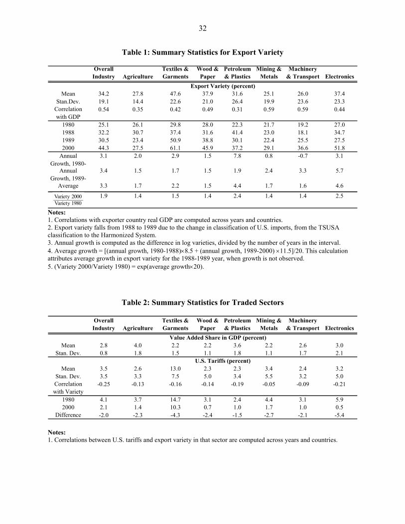
Summary statistics for the measure of export variety in (32) are provided in Table 1.
There is a strong correlations with real GDP in the exporting countries, shown in the third row.
In the next rows we show export variety in each sector for 1980, 1988, 1989 and 2000. There is a
discrete fall in export variety from 1988 to 1989, due to the changing classification of U.S.
import statistics from the TSUSA to the HS classification. We will account for that discrete fall
10 We thank a referee for pointing this out that this consistency was needed. If we instead use the worldwide exports to the U.S. in each year as the comparison, then the measures of export variety obtained are somewhat higher than those reported in Table 1.
18
by including year fixed-effects in all our estimating equations. Taking the growth rate of export
variety over 1980-1988 and 1989-2000, the average growth is 3.3% per year, which means that
export variety increases by 1.9 times over the two decades.11 That average growth and total
increase are shown in the final rows of Table 1, and are lower in the agriculture sector, wood and
paper, and mining and metals, but higher in the electronics industry.
3.4 Other Data
Our data set is an unbalanced panel of 48 countries from 1980 to 2000, a total of 532
observations. The GDP and endowment data are obtained from World Development Indicators
(World Bank, 2005). Real GDP is measured in constant 2000 U.S. dollars (converted at nominal
exchange rates that year), so we are using GDP deflators to measure htP and .RGDPh
t There are
three primary factor endowments: labor, capital and agriculture land. Labor is defined as the
number of persons in the labor force of each country. Capital is constructed from real investment
using the perpetual inventory method.12 Endowments of the comparison country F are measured
by the sum of endowments for all sample countries, ∑ == H
1hhkt
Fkt vv .
We aggregate goods into N = 7 sectors, as shown in Tables 1 and 2. The value added of
these sectors are available in a UNIDO data set, used to construct the value added share of each
sector, hits . The 8th sector is the nontraded good, with price h
t8ψ obtained by netting the prices of
traded goods, both export and import, from the country GDP deflators. This procedure may
11 The highest growth rates of export variety are shown by Turkey, Iceland, Bulgaria, and Thailand, which start with very low variety. The lowest growth rates are shown by Peru, Canada, Sweden, the U.K. and Japan, which start with high variety (except for Peru). Israel, South Korea, Costa Rica, Ireland and Singapore have growth rates of export variety to the U.S. of 2.5%, 2.7%, 3.3%, 3.9% and 4.6% per year, respectively. 12 Real investment is obtained by deflating the gross domestic capital formation of countries with that item’s GDP deflator. In addition, we construct the base year capital stock using an infinite sum series of investment prior to the first year, assuming that the growth rate of investment in the first five years proxy investment prior to the first year.
19
introduce some errors into the nontraded price, which we address using instrumental variables.13
In Table 2 we show the sectoral shares for each traded sector, which jointly account for
20% of GDP on average. Instruments used to address the endogeneity of export variety, as well
as measurement error in the nontraded prices, consist of U.S. tariffs with each partner country,
free trade agreements and distance to the U.S. The U.S. tariffs vary by sector, countries and
years, and are summarized in Table 2. The textiles and garments sector has the highest tariffs,
and a correlation of –0.16 with export variety. In the final rows of Table 2 we also show the drop
in tariffs from 1980-2000, which are modest in size: –5.4 percentage points in electronics, and
less than that in all other sectors. The small cuts in U.S. tariffs means that this variable will not
be able to account for the large growth in export variety.
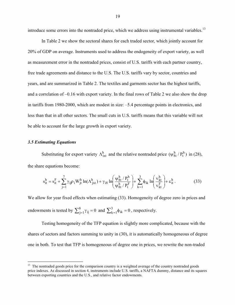
3.5 Estimating Equations
Substituting for export variety hixtΛ and the relative nontraded price )P/( h
tht8ψ in (28),
the share equations become:
∑ ∑= =
ε+⎟⎟⎠
⎞⎜⎜⎝
⎛φ+⎟
⎟⎠
⎞⎜⎜⎝
⎛
ψ
ψγ+Λργ+=
7
1j
3
1k
hitF
kt
hkt
ikFt
ht8
ht
ht8
8ihjxt
hjtiij
Fit
hit v
vlnP/P/ln)ln(Wss . (33)
We allow for year fixed effects when estimating (33). Homogeneity of degree zero in prices and
endowments is tested by 081j ij =γ∑ = and 03
1k ik =φ∑ = , respectively.
Testing homogeneity of the TFP equation is slightly more complicated, because with the
shares of sectors and factors summing to unity in (30), it is automatically homogeneous of degree
one in both. To test that TFP is homogeneous of degree one in prices, we rewrite the non-traded
13 The nontraded goods price for the comparison country is a weighted average of the country nontraded goods price indexes. As discussed in section 4, instruments include U.S. tariffs, a NAFTA dummy, distance and its squares between exporting countries and the U.S., and relative factor endowments.
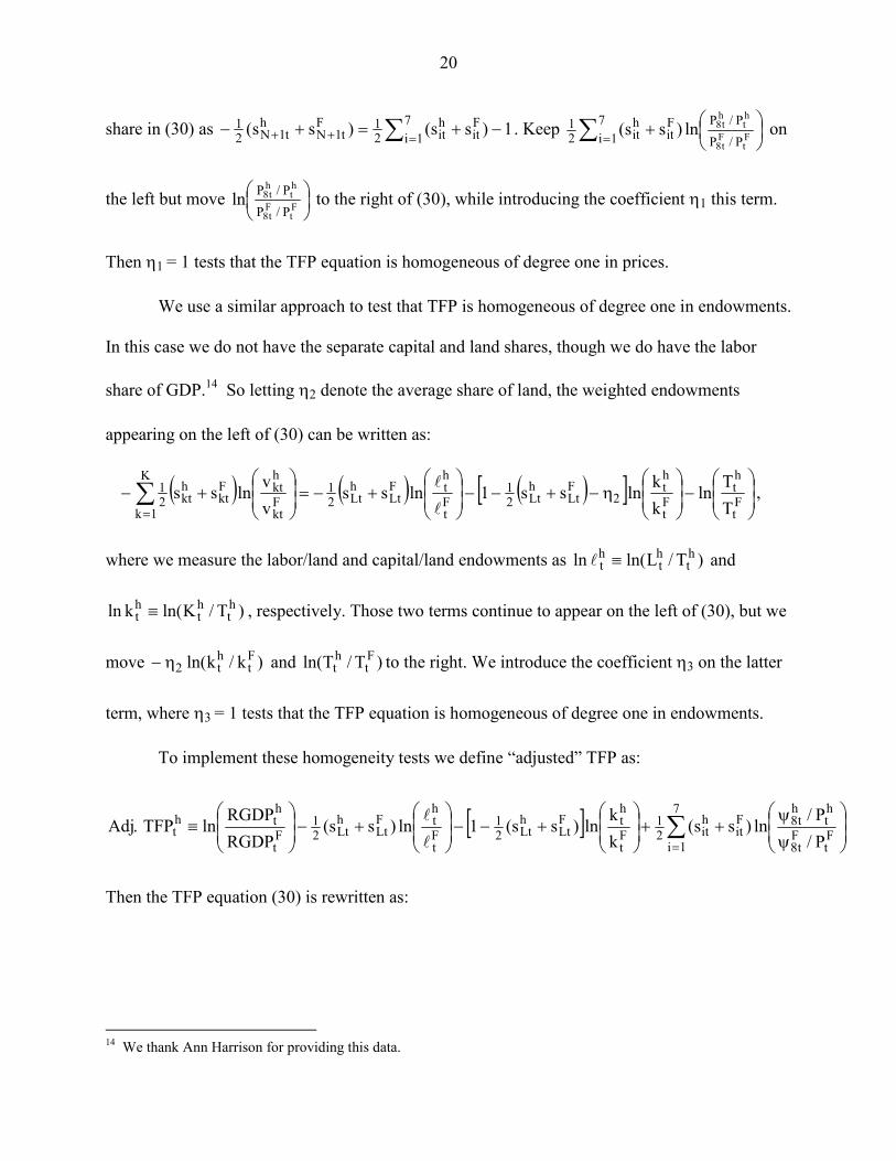
20
share in (30) as ∑ =++ −+=+− 71i
Fit
hit2
1Ft1N
ht1N2
1 1)ss()ss( . Keep ⎟⎠⎞
⎜⎝⎛+∑ = F
tFt8
ht
ht8
P/PP/P7
1iFit
hit2
1 ln)ss( on
the left but move ⎟⎠⎞
⎜⎝⎛
Ft
Ft8
ht
ht8
P/PP/Pln to the right of (30), while introducing the coefficient η1 this term.
Then η1 = 1 tests that the TFP equation is homogeneous of degree one in prices.
We use a similar approach to test that TFP is homogeneous of degree one in endowments.
In this case we do not have the separate capital and land shares, though we do have the labor
share of GDP.14 So letting η2 denote the average share of land, the weighted endowments
appearing on the left of (30) can be written as:
( ) ( ) ( )[ ] ⎟⎟⎠
⎞⎜⎜⎝
⎛−⎟
⎟⎠
⎞⎜⎜⎝
⎛η−+−−⎟
⎟⎠
⎞⎜⎜⎝
⎛+−=⎟
⎟⎠
⎞⎜⎜⎝
⎛+− ∑
=Ft
ht
Ft
ht
2FLt
hLt2
1Ft
htF
LthLt2
1K
1kFkt
hktF
kthkt2
1
TTln
kklnss1lnss
vvlnss
l
l ,
where we measure the labor/land and capital/land endowments as )T/Lln(ln ht
ht
ht ≡l and
)T/Kln(kln ht
ht
ht ≡ , respectively. Those two terms continue to appear on the left of (30), but we
move )k/kln( Ft
ht2η− and )T/Tln( F
tht to the right. We introduce the coefficient η3 on the latter
term, where η3 = 1 tests that the TFP equation is homogeneous of degree one in endowments.
To implement these homogeneity tests we define “adjusted” TFP as:
[ ] ⎟⎟⎠
⎞⎜⎜⎝
⎛
ψψ
++⎟⎟⎠
⎞⎜⎜⎝
⎛+−−⎟
⎟⎠
⎞⎜⎜⎝
⎛+−⎟
⎟⎠
⎞⎜⎜⎝
⎛≡ ∑
=Ft
Ft8
ht
ht8
7
1i
Fit
hit2
1Ft
htF
LthLt2
1Ft
htF
LthLt2
1Ft
hth
t P/P/ln)ss(
kkln)ss(1ln)ss(
RGDPRGDPlnTFP.Adj
l
l
Then the TFP equation (30) is rewritten as:
14 We thank Ann Harrison for providing this data.
21
.)ln(W)ss(
TTln
kkln
P/P/lnTFP.Adj
ht
7
1i
hixt
hiti
Fit
hit2
1
Ft
ht
3Ft
ht
2Ft
Ft8
ht
ht8
1t0h0
ht
ε+Λρ++
⎟⎟⎠
⎞⎜⎜⎝
⎛η+⎟
⎟⎠
⎞⎜⎜⎝
⎛η−⎟
⎟⎠
⎞⎜⎜⎝
⎛
ψψ
η+β+α=
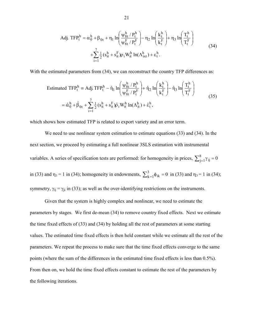
∑=
(34)
With the estimated parameters from (34), we can reconstruct the country TFP differences as:
,ˆ)ln(Wˆ)ss(ˆˆ
TTlnˆ
kklnˆ
P/P/lnˆTFP.AdjTFPEstimated
ht
7
1i
hit
hiti
Fit
hit2
1t0
h0
Ft
ht
3Ft
ht
2Ft
Ft8
ht
ht8
1ht
ht
ε+Λρ++β+α=
⎟⎟⎠
⎞⎜⎜⎝
⎛η−⎟
⎟⎠
⎞⎜⎜⎝
⎛η+⎟
⎟⎠
⎞⎜⎜⎝
⎛
ψψ
η−≡
∑=
(35)
which shows how estimated TFP is related to export variety and an error term.
We need to use nonlinear system estimation to estimate equations (33) and (34). In the
next section, we proceed by estimating a full nonlinear 3SLS estimation with instrumental
variables. A series of specification tests are performed: for homogeneity in prices, 081j ij =γ∑ =
in (33) and η1 = 1 in (34); homogeneity in endowments, 031k ik =φ∑ = in (33) and η3 = 1 in (34);
symmetry, γij = γji in (33); as well as the over-identifying restrictions on the instruments.
Given that the system is highly complex and nonlinear, we need to estimate the
parameters by stages. We first de-mean (34) to remove country fixed effects. Next we estimate
the time fixed effects of (33) and (34) by holding all the rest of parameters at some starting
values. The estimated time fixed effects is then held constant while we estimate all the rest of the
parameters. We repeat the process to make sure that the time fixed effects converge to the same
points (where the sum of the differences in the estimated time fixed effects is less than 0.5%).
From then on, we hold the time fixed effects constant to estimate the rest of the parameters by
the following iterations.
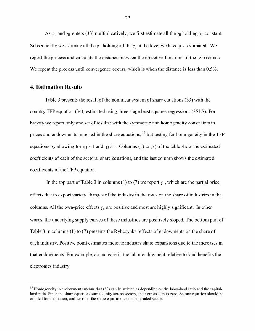
22
As ρi and γij enters (33) multiplicatively, we first estimate all the γij holding ρi constant.
Subsequently we estimate all the ρi holding all the γij at the level we have just estimated. We
repeat the process and calculate the distance between the objective functions of the two rounds.
We repeat the process until convergence occurs, which is when the distance is less than 0.5%.
4. Estimation Results
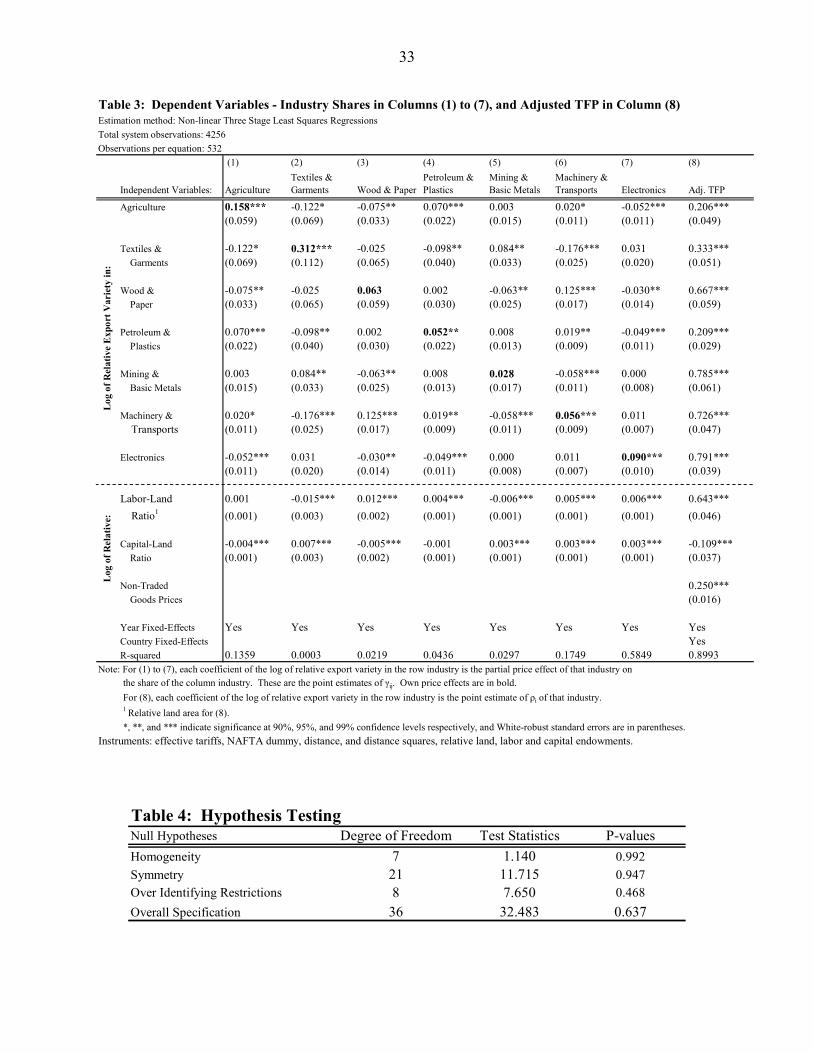
Table 3 presents the result of the nonlinear system of share equations (33) with the
country TFP equation (34), estimated using three stage least squares regressions (3SLS). For
brevity we report only one set of results: with the symmetric and homogeneity constraints in
prices and endowments imposed in the share equations, 15 but testing for homogeneity in the TFP
equations by allowing for η1 ≠ 1 and η3 ≠ 1. Columns (1) to (7) of the table show the estimated
coefficients of each of the sectoral share equations, and the last column shows the estimated
coefficients of the TFP equation.
In the top part of Table 3 in columns (1) to (7) we report γij, which are the partial price
effects due to export variety changes of the industry in the rows on the share of industries in the
columns. All the own-price effects γjj are positive and most are highly significant. In other
words, the underlying supply curves of these industries are positively sloped. The bottom part of
Table 3 in columns (1) to (7) presents the Rybczynksi effects of endowments on the share of
each industry. Positive point estimates indicate industry share expansions due to the increases in
that endowments. For example, an increase in the labor endowment relative to land benefits the
electronics industry.
15 Homogeneity in endowments means that (33) can be written as depending on the labor-land ratio and the capital-land ratio. Since the share equations sum to unity across sectors, their errors sum to zero. So one equation should be omitted for estimation, and we omit the share equation for the nontraded sector.
23
The top half of column (8) in Table 3 presents the 3SLS estimates of ρi = (σi – 1)/θiσi for
each sector. All the point estimates are positive, and are smaller than one, implying that the
elasticities of substitution exceed unity and that the restriction 1ii −σ>θ in (12) holds. The
industry with the highest value of ρi = 0.791 is electronics, so that increases in export variety
contribute the most to country productivity, whereas the industry with the lowest value of ρi =
0.206 is agriculture, so export variety contributes little to productivity. While we cannot
separately identify the elasticity of substitution from the Pareto parameter iθ , one interpretation
of these findings is that agriculture has a high value of σi, or a high value of iθ as compared to
./)1( ii σ−σ High σi means homogeneous products, whereas high iθ means there is little
dispersion in firm productivities, both of which seem appropriate for agriculture. The low value
of ρi for electronics can be explained by heterogeneous products (low σi) or a wide dispersion of
productivities (low iθ as compared to ii /)1( σ−σ ), which again seem reasonable.
The coefficient of the capital-land ratio in the lower part of column (8) in Table 3, which
has the interpretation of the negative share of land in GDP is about 11 percent. The coefficient on
the relative land size (shown in the labor-land row) is statistically less than one, which implies
that homogeneity in factor endowments is rejected. Likewise, the coefficient η1 on the price of
nontraded goods is significantly less than one, which violates the homogeneity constraint on
prices in the TFP equation.
Instruments used in Table 3 consisting of U.S. tariffs for textiles and apparels (the
industry are among most protected) varying by source country and year, a NAFTA dummy,
distance and its squares between exporting countries and the U.S. (in kilometers), and relative
24
endowments. We did not include transport costs to the U.S. due to their potential endogeneity.16
Given that the above nonlinear 3SLS estimation involves minimizing the criterion function, the
minimized value provides a test statistic for hypothesis testing. The difference between the
values of the criterion functions of the restricted and unrestricted models is asymptotically chi-
squared distributed with degree of freedom equal to the number of restrictions. According to
Davidson and MacKinnon (1993, p. 665), it is important that the same estimate of variance-
covariance matrix be used for both the restricted and unrestricted estimations, in order to ensure
that the test statistic is positive. We use the variance-covariance matrix of the unrestricted model.
Table 4 presents the test statistics and the associated p-values of the hypothesis tests.
First, we test the homogeneity constraints on prices and endowments in the share equations,
along with the homogeneity constraint in endowments in the TFP equation. As shown in the first
row of Table 4, these homogeneity constraints are not rejected. If we also test the homogeneity
constraint on prices in the TFP equation (i.e. η1 = 1), that constraint is easily rejected, possibly
due to measurement errors in nontraded good prices. So that constraint is not imposed.
Next, the twenty-one symmetry constraints on the cross-price effects are tested on the
whole system, which are not rejected. Third, we test for the 8 over-identifying restrictions due to
the extra instruments, which are not rejected. Finally, the overall specification of the system is
tested by jointly testing all these 36 constraints. This is done by comparing the value of criterion
function of the restricted model to a just-identified model with no symmetry constraints and no
extra instruments. The whole set of restriction are again not rejected, which supports the
symmetry and homogeneity constraints and the validity of instruments. In the next section we
explore the instruments further by reporting their regressions with export variety.
16 Countries that trade more with the U.S. may have lower transport costs as a result, as noted by a referee.
25
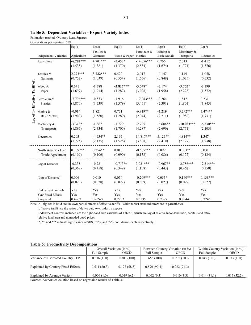
4.1 Effects of Tariffs and Distance on Export Variety
Table 5 presents least squares (LS) estimation linking export variety to all instruments
and exogenous variables of the nonlinear 3SLS system presented in Table 3. This is similar but
not identical to the first-stage estimation of the nonlinear system, which involves regressing the
derivatives of each equation with respect to the parameters of the system on all the instruments
and exogenous variables. In comparison, the regressions we present in Table 5 just uses the
export variety index hitlnΛ as a dependent variable, which allows us to see the relationship
between export variety and the tariff and distance variables.
The top part of Table 5 shows the effects of U.S. tariffs on the export variety of the
industry in the columns. We expect industry export variety to decrease with its own tariff, while
there may exist some positive effects (due to reallocation of resources among industries) when
there is a tariff increase in other industries. All industry export variety indexes are negatively
correlated with own tariffs except for the textiles & garments and the electronics industries. For
textiles & garments, the positive effect of tariffs on export variety could be due to the influence
of MFA quotas, which are known to be more restrictive and binding than tariffs. For the
electronics industry, it could be the case that other features (such as non-tariff barriers and skilled
labor endowments) are more important in explaining expansion in export variety than tariffs.
A one percentage point increase in U.S. tariffs on petroleum and plastics lowers export
variety of that industry by 17%, at the highest, and a similar increase in the wood and paper tariff
lowers export variety of the industry by 3.8%, at the lowest. While these semi-elasticities show
that tariffs have a statistically significant impact on product variety in most industries, the
economic magnitude of this effect is very modest. From the last rows of Table 2, we know that
the observed drop in U.S. tariffs over 1980-2000 are quite small. Using these tariff reductions
26
and the semi-elasticities in Table 5, we can calculate that the drop in U.S. tariffs has increased
export variety by only 8.3% over the two decades (or 28% if we ignore the estimates for the
textiles and garments and electronics industries). Recalling that average export variety increased
by 1.9 times over 1980-2000 (from Table 1), we conclude that fall in U.S. tariffs explains only a
very small part of export variety growth.
The next section of Table 5 shows the marginal effects of NAFTA on export variety.
Given that we already control for tariffs, these variables capture the effect of the reduction in
non-tariff barriers due to the signing of such agreements on export variety. NAFTA is shown to
have significant positive effects on the export variety of agriculture, textiles & garments and
machinery and transport equipment, and has a significant negative effect on the export variety of
the petroleum and plastics industry.
The third section of Table 5 relates distance (in log of kilometers) and its squares to the
export variety of the industries. Overall, the further a country is from the U.S., the less variety is
exported. Such negative effects are particularly significant for the machinery and transport
equipment industry, as well as the electronics industry. However, the effects are not linear since
the coefficients on distance squares are mostly positive, which indicates that that marginal effect
of each addition kilometer diminishes with the overall distance between the two countries. Other
than tariffs, distance and its squares, we have also included all the right-hand side exogenous
variables in Table 3 in the regressions. These variables are a full set of year fixed effects, the
labor-land ratio, capital-land ratio, non-traded goods prices, and land area. The vast majority of
the increase in export variety over time is explained by the year fixed effects, while the other
variables explain its variation across countries. This result could indicate that the falling fixed
costs of exporting that are common across countries, such as the modernization of container
27
ports, faster and better shipping lines, are the main factors behind the expansion in export
variety. We leave an exploration of that possibility for future research.
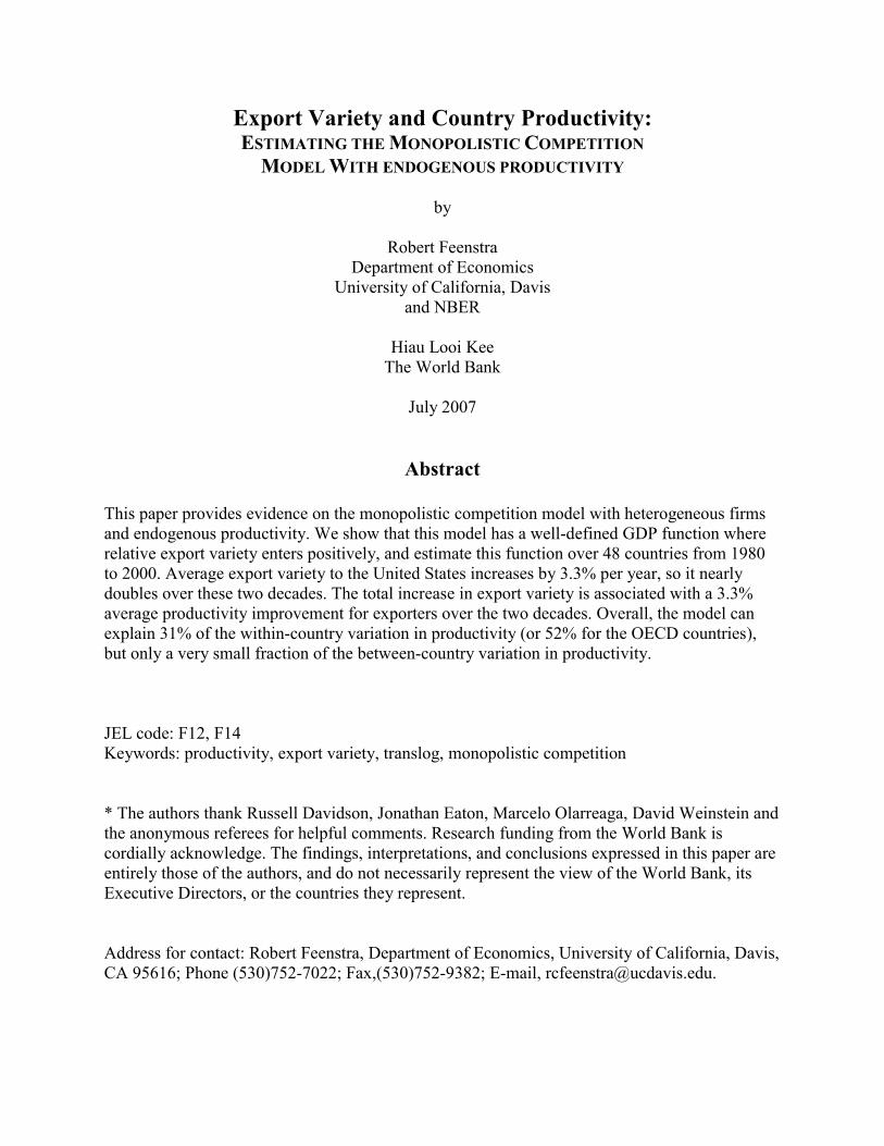
4.3 Productivity Decomposition
To gain additional insight into the links between export variety and country productivity,
we performed panel regressions of estimated productivity on export variety (constructed from the
estimates in Table 3). As in (35), we regress estimated country TFP to that portion due to export
variety, ∑ =Λρ+7
1ihititi
Fit
hit2
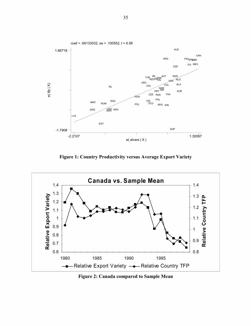
1 )ln(Wˆ)ss( . Figure 1 plots the scatter graph of country TFP against
industry export variety. Both variables are averaged over time so this scatter plot is equivalent to
a “between” regression. It is evident that export variety has significant explanatory power for the
variation of the country productivity differences: R2=0.48 for this univariate regression. The
problem with this “between” regression, however, is that it omits country fixed-effects, which
should be included to reflect exogenous technological progress across countries.
Running panel regressions including country and time fixed effects, as in (34), in Table 6
we report the amount of variance explained by each term. In the total sample, export variety can
explain 1% of the overall variation in country TFP, along with 31.1% of within-country TFP
variation, but only 0.3% of the between-country variation. Thus, export variety is strongly
correlated with the variation in country TFP over time, but explains only a tiny fraction of the
variation in TFP across countries. This finding continues to hold if we investigate only the
OECD countries (using the same parameters estimates as in Table 3). In that case, export variety
explains 6.2% of the overall variation in country TFP, and 52.2% of the within-country TFP
variation, but just 3.3% of the between-country variation.
To further illustrate the effects of export variety on country productivity, according to
(34), a 1% increase in the export variety of each industry would increase country productivity by
28
hiti
Fit
hit2
1 Wˆ)ss( ρ+ percent. Thus, we can compute that at the sample mean, a doubling of export
varieties of all industries could lead to 3.6% increase in country productivity. This effect is
significant both statistically and economically. It implies that the 1.9 times expansion of export
variety over 1980-2000 explains a 3.3% increase in exporters’ productivity. Recall that average
export variety itself also increased by 3.3% per year. So as a rule-of-thumb, our estimates show
that a sustained increase of x% per annum in export variety over two decades leads to a x%
overall productivity improvement for the exporter.17 This is an estimate of the endogenous
portion of productivity gains that is consistent with the monopolistic competition model. As
noted above, however, the variety increase itself is not well-explained by the marginal trade costs
such as tariff cuts or other variables that change over countries and time; instead, the increase in
export variety is predicted mainly by the time fixed effects. In this sense, our results do not give
a full account of the mechanism of increased export activity and resulting productivity growth in
the monopolistic competition model.
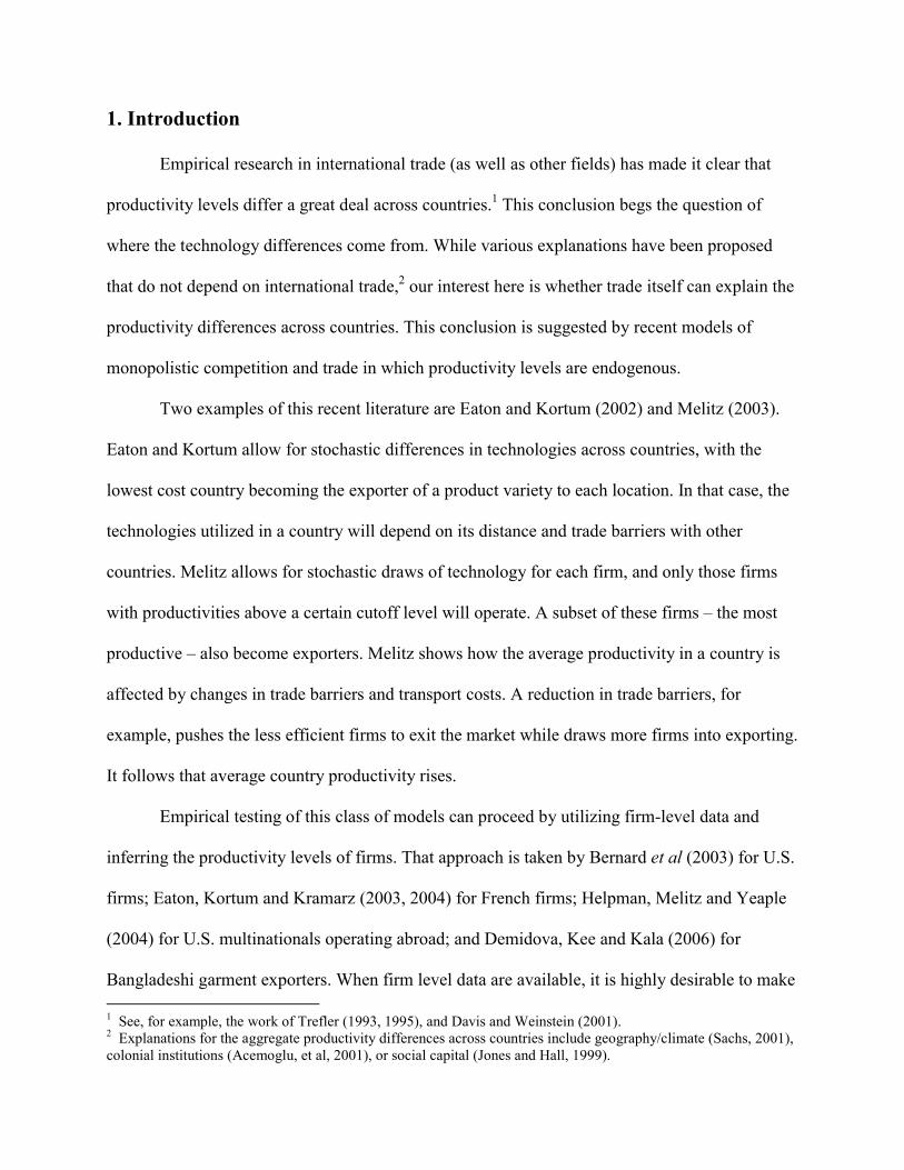
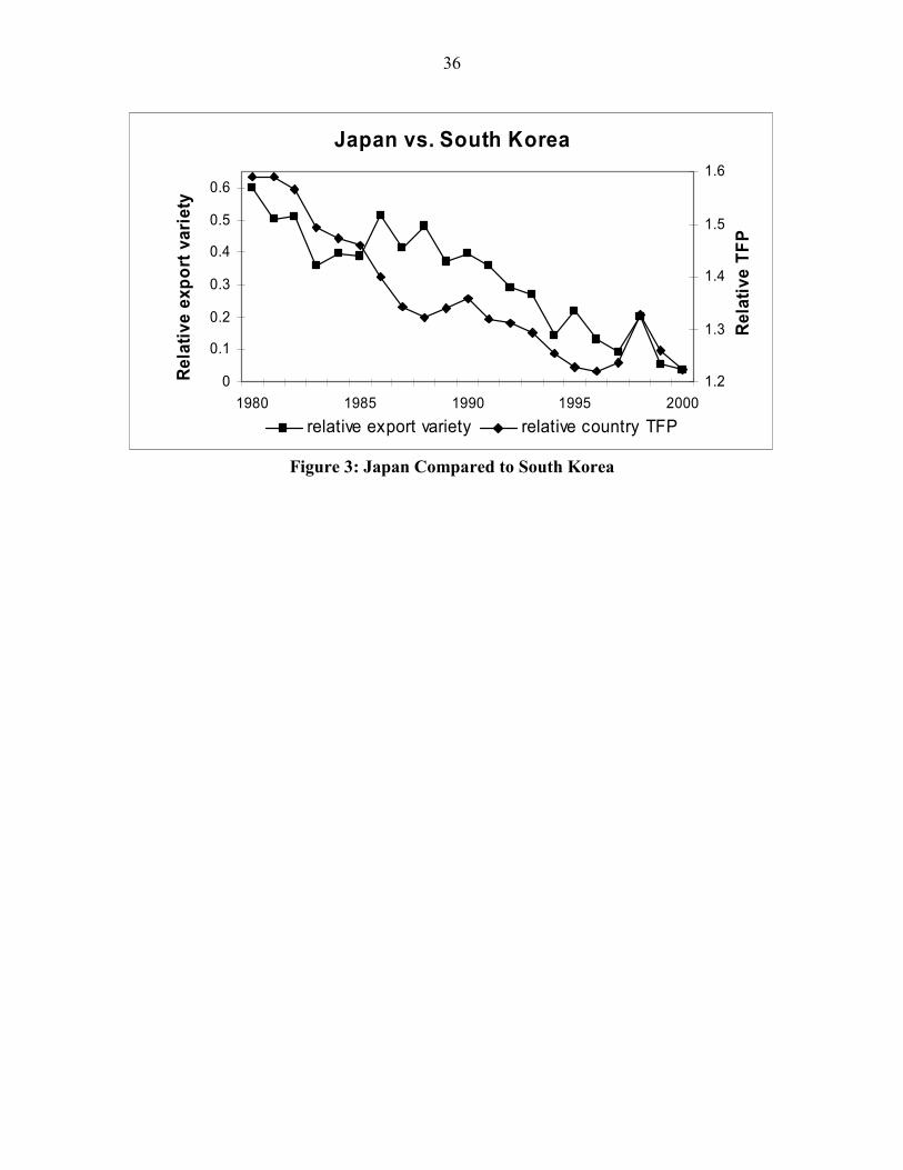
The time series linkage between export variety and productivity can be seen from Figures
3 and 4. Figure 3 compares Canada to the sample mean in terms of productivity, and average
export variety, from 1980 to 2000. The relative export variety index is measured on the vertical
left-hand scale, while relative country TFP index is measured on the right-hand scale. It is clear
that these two series move together closely. In the years just after the Canada-U.S. free trade
agreement in 1989, Canada has a boost in its export variety to the U.S. and in its TFP, but
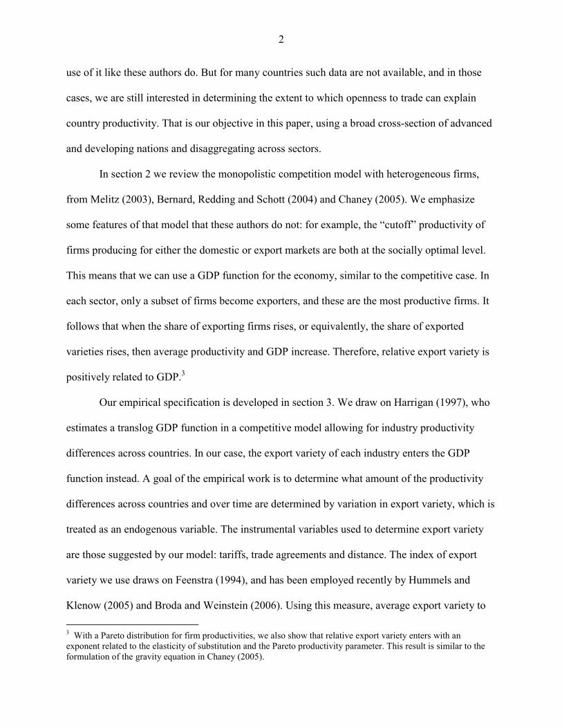
afterwards experienced a decline in both indexes relative to other countries. Figure 4 compares
Japan to South Korea. Similar to the previous figure, average export variety is measured on the
17 The countries with highest growth of export variety to the U.S., of 7.4 – 11% per year, are listed in note 11, and the countries with lowest variety growth (0.8% for Peru and 1.0 – 1.6% for the others) are also listed there. The implied country productivity growth over 1980-2000 will differ from these magnitudes to the extent that the export and value-added shares of these countries deviate from the sample averages.
29
left-hand scale, while the productivity of Japan relative to Korea is measured on the right-hand
scale. The movements of the two lines suggest that over the twenty year period, South Korea is
catching up in terms of export variety as well as country productivity.
5. Conclusions
Current research in international trade (Melitz, 2003) has stressed that productivity is
endogenous through the self-selection of exporters: exporters are more productive on average
than domestic firms, so an increase in export activity is associated with rising productivity. In
this paper we have attempted to estimate the relation between export variety and productivity
using a GDP function across countries and over time. We have shown that a CES measure of
export variety enters the GDP function like a sectoral “price”. We have treated export variety as
an endogenous variable, and as instruments use those suggested by Melitz (2003): tariffs, trade
agreements and distance.
The measure of export variety we use is constructed to be consistent across countries and
over time. It shows an average 3.3% per annum increase in export variety to the U.S. over 1980-
2000. Only a small amount of that increase is explained by observed cuts in U.S. tariffs.
Corresponding to the 3.3% sustained growth in export variety over two decades is a 3.3%
productivity gain in the exporting countries. That estimate is larger than the gains to the U.S.
from increased import variety over 1972-2001, which amount to 2.6% of GDP in 2001 according
to Broda and Weinstein (2005). Our estimate can be interpreted as the endogenous portion of
productivity gains for exporters (with the caveat that the variety increase itself is not well-
explained by tariff cuts). Overall, the model can explain 31.1% of the within-country variation in
productivity (or 52.2% for the OECD countries), but only a very small fraction of between-
country variation. We conclude that export variety in the monopolistic competition model with
30
heterogeneous firms is quite effective at accounting for the time-series variation in productivity,
but not the large absolute differences in productivity between countries.
References
Acemoglu, Daron, Simon Johnson and James A. Robinson, 2001. The colonial origins of comparative development: An empirical investigation. American Economic Review, 91(5), December, 1369-1401.
Bernard, Andrew, Jonathan Eaton, J. Bradford Jensen and Samuel Kortum, 2003. Plants and
productivity in international trade. American Economic Review, 93, September, 1268-1290.
Bernard, Andrew, Stephen Redding and Peter Schott, 2004. Comparative advantage and
heterogeneous firms. NBER Working Paper no. 10668. Broda, Christian and David Weinstein, 2006. Globalization and the gains from variety. Quarterly
Journal of Economics, May 2006, 121(2), 541-585. Chaney, Thomas, 2005. Distorted gravity: Heterogenous firms, market structure and the
geography of international trade, University of Chicago. Davidson, Russell and James MacKinnon, 1993. Estimation and Inferences in Econometrics.
Oxford University Press. Demidova, Svetlana, Hiau Looi Kee and Kala Krishna, 2006. Do trade policy differences induce
sorting? Theory and evidence from Bangladeshi apparel exporters. NBER Working Paper no. 12725.
Dixit, Avinash K. and Joseph E. Stiglitz, 1977. Monopolistic competition and optimum product
diversity. American Economic Review, 67(3), June, 297-308. Eaton, Jonathan and Samuel Kortum, 2002. Technology, geography and trade. Econometrica,
70(5), September, 1741-1780. Eaton, Jonathan, Samuel Kortum and Francis Kramarz, 2003. An anatomy of international trade:
evidence from French firms, University of New York, University of Chicago and CREST, unpublished.
Eaton, Jonathan, Samuel Kortum and Francis Kramarz, 2004. Dissecting trade: firms, industries,
and export destinations. American Economic Review, 94(2), 150-154. Feenstra, Robert C., 1994. New product varieties and the measurement of international prices.
American Economic Review, 84(1), 157-177.
31
Feenstra, Robert C., 2004. Advanced International Trade: Theory and Evidence. Princeton
University Press. Feenstra, Robert C. and Hiau Looi Kee, 2004. On the measurement of product variety in trade.
American Economic Review, 94(2), 145-149. Harrigan, James, 1997. Technology, factor supplies, and international specialization: Estimating
the neoclassical model. American Economic Review, 87(3), 475-494. Helpman, Elhanan and Paul Krugman, 1985. Market Structure and Foreign Trade. Cambridge:
MIT Press. Helpman, Elhanan, Marc Melitz and Stephen Yeaple, 2004. Exports vs. FDI with heterogeneous
firms. American Economic Review, March, 300-316. Hummels, David and Peter Klenow, 2005. The variety and quality of a nation’s trade. American
Economic Review, 95(3), June, 704-723. Jones, Charles I. and Robert E. Hall, 1999. Why do some countries produce so much more
output per worker than others? Quarterly Journal of Economics, 116(1), 83-116. Melitz, Marc J., 2003. The impact of trade on intra-industry reallocations and aggregate industry
productivity. Econometrica, 71(6),1695-1725. Sachs, Jeffrey D., 2001. Tropical underdevelopment, NBER Working Paper no. 8119. Sato, Kazuo, 1976. The ideal log-change index number. Review of Economics and Statistics 58,
May, 223-228. Trefler, Daniel, 1993. International factor price differences: Leontief was right! Journal of
Political Economy, December, 101(6), 961-987. Trefler, Daniel, 1995. The case of missing trade and other mysteries, American Economic
Review, December, 85(5), 1029-1046. Vartia, Y.O., 1976. Ideal log-change index numbers. Scandinavian Journal of Statistics 3, 121-
126.
32
Table 1: Summary Statistics for Export Variety
Overall Industry Agriculture
Textiles & Garments
Wood & Paper
Petroleum & Plastics
Mining & Metals
Machinery & Transport Electronics
Mean 34.2 27.8 47.6 37.9 31.6 25.1 26.0 37.4Stan.Dev. 19.1 14.4 22.6 21.0 26.4 19.9 23.6 23.3
Correlation with GDP
0.54 0.35 0.42 0.49 0.31 0.59 0.59 0.44
1980 25.1 26.1 29.8 28.0 22.3 21.7 19.2 27.01988 32.2 30.7 37.4 31.6 41.4 23.0 18.1 34.71989 30.5 23.4 50.9 38.8 30.1 22.4 25.5 27.52000 44.3 27.5 61.1 45.9 37.2 29.1 36.6 51.8
Annual Growth, 1980-
3.1 2.0 2.9 1.5 7.8 0.8 -0.7 3.1
Annual Growth, 1989-
3.4 1.5 1.7 1.5 1.9 2.4 3.3 5.7
Average G h
3.3 1.7 2.2 1.5 4.4 1.7 1.6 4.6
1.9 1.4 1.5 1.4 2.4 1.4 1.4 2.5
Export Variety (percent)
1980Variety2000Variety
Notes: 1. Correlations with exporter country real GDP are computed across years and countries. 2. Export variety falls from 1988 to 1989 due to the change in classification of U.S. imports, from the TSUSA classification to the Harmonized System. 3. Annual growth is computed as the difference in log varieties, divided by the number of years in the interval. 4. Average growth = [(annual growth, 1980-1988)×8.5 + (annual growth, 1989-2000) ×11.5]/20. This calculation attributes average growth in export variety for the 1988-1989 year, when growth is not observed. 5. (Variety 2000/Variety 1980) = exp(average growth×20).
Table 2: Summary Statistics for Traded Sectors
Overall Industry Agriculture
Textiles & Garments
Wood & Paper
Petroleum & Plastics
Mining & Metals
Machinery & Transport Electronics
Value Added Share in GDP (percent)Mean 2.8 4.0 2.2 2.2 3.6 2.2 2.6 3.0
Stan. Dev. 0.8 1.8 1.5 1.1 1.8 1.1 1.7 2.1
Mean 3.5 2.6 13.0 2.3 2.3 3.4 2.4 3.2Stan. Dev. 3.5 3.3 7.5 5.0 3.4 5.5 3.2 5.0Correlation with Variety
-0.25 -0.13 -0.16 -0.14 -0.19 -0.05 -0.09 -0.21
1980 4.1 3.7 14.7 3.1 2.4 4.4 3.1 5.92000 2.1 1.4 10.3 0.7 1.0 1.7 1.0 0.5
Difference -2.0 -2.3 -4.3 -2.4 -1.5 -2.7 -2.1 -5.4
U.S. Tariffs (percent)
Notes: 1. Correlations between U.S. tariffs and export variety in that sector are computed across years and countries.
33
Table 3: Dependent Variables - Industry Shares in Columns (1) to (7), and Adjusted TFP in Column (8)Estimation method: Non-linear Three Stage Least Squares RegressionsTotal system observations: 4256Observations per equation: 532
(1) (2) (3) (4) (5) (6) (7) (8)
Independent Variables: AgricultureTextiles & Garments Wood & Paper
Petroleum & Plastics
Mining & Basic Metals
Machinery & Transports Electronics Adj. TFP
Agriculture 0.158*** -0.122* -0.075** 0.070*** 0.003 0.020* -0.052*** 0.206***(0.059) (0.069) (0.033) (0.022) (0.015) (0.011) (0.011) (0.049)
Textiles & -0.122* 0.312*** -0.025 -0.098** 0.084** -0.176*** 0.031 0.333*** Garments (0.069) (0.112) (0.065) (0.040) (0.033) (0.025) (0.020) (0.051)
Wood & -0.075** -0.025 0.063 0.002 -0.063** 0.125*** -0.030** 0.667*** Paper (0.033) (0.065) (0.059) (0.030) (0.025) (0.017) (0.014) (0.059)
Petroleum & 0.070*** -0.098** 0.002 0.052** 0.008 0.019** -0.049*** 0.209*** Plastics (0.022) (0.040) (0.030) (0.022) (0.013) (0.009) (0.011) (0.029)
Mining & 0.003 0.084** -0.063** 0.008 0.028 -0.058*** 0.000 0.785*** Basic Metals (0.015) (0.033) (0.025) (0.013) (0.017) (0.011) (0.008) (0.061)
Machinery & 0.020* -0.176*** 0.125*** 0.019** -0.058*** 0.056*** 0.011 0.726*** Transports (0.011) (0.025) (0.017) (0.009) (0.011) (0.009) (0.007) (0.047)
Electronics -0.052*** 0.031 -0.030** -0.049*** 0.000 0.011 0.090*** 0.791***(0.011) (0.020) (0.014) (0.011) (0.008) (0.007) (0.010) (0.039)
Labor-Land 0.001 -0.015*** 0.012*** 0.004*** -0.006*** 0.005*** 0.006*** 0.643*** Ratio1 (0.001) (0.003) (0.002) (0.001) (0.001) (0.001) (0.001) (0.046)
Capital-Land -0.004*** 0.007*** -0.005*** -0.001 0.003*** 0.003*** 0.003*** -0.109*** Ratio (0.001) (0.003) (0.002) (0.001) (0.001) (0.001) (0.001) (0.037)
Non-Traded 0.250*** Goods Prices (0.016)
Year Fixed-Effects Yes Yes Yes Yes Yes Yes Yes YesCountry Fixed-Effects YesR-squared 0.1359 0.0003 0.0219 0.0436 0.0297 0.1749 0.5849 0.8993
Note: For (1) to (7), each coefficient of the log of relative export variety in the row industry is the partial price effect of that industry on the share of the column industry. These are the point estimates of γij. Own price effects are in bold. For (8), each coefficient of the log of relative export variety in the row industry is the point estimate of ρi of that industry. 1 Relative land area for (8). *, **, and *** indicate significance at 90%, 95%, and 99% confidence levels respectively, and White-robust standard errors are in parentheses.Instruments: effective tariffs, NAFTA dummy, distance, and distance squares, relative land, labor and capital endowments.
Log
of R
elat
ive:
Log
of R
elat
ive
Exp
ort V
arie
ty in
:
Table 4: Hypothesis TestingNull Hypotheses Degree of Freedom Test Statistics P-valuesHomogeneity 7 1.140 0.992Symmetry 21 11.715 0.947Over Identifying Restrictions 8 7.650 0.468Overall Specification 36 32.483 0.637
34
Table 5: Dependent Variables - Export Variety IndexEstimation method: Ordinary Least SquaresObservations per equation: 509
Eq (1) Eq(2) Eq(3) Eq(4) Eq(5) Eq(6) Eq(7)
Independent Variables: AgricultureTextiles & Garments Wood & Paper
Petroleum & Plastics
Mining & Basic Metals
Machinery & Transports Electronics
Agriculture -6.282*** 4.701*** -2.453* -14.056*** 0.766 2.013 -1.412(1.535) (1.381) (1.370) (2.534) (1.674) (1.771) (1.376)
Textiles & 2.273*** 3.732*** 0.522 -2.017 -0.147 1.149 -1.058 Garments (0.752) (1.039) (0.554) (1.666) (0.849) (1.025) (0.632)
Wood & 0.641 -1.788 -3.817*** -5.648* -3.174 -3.762* -2.199 Paper (1.697) (1.914) (1.287) (3.028) (1.958) (2.228) (1.572)
Petroleum & -7.796*** -0.573 -1.916 -17.063*** -2.264 1.812 0.231 Plastics (1.870) (1.739) (1.379) (3.461) (2.391) (1.801) (1.843)
Mining & -0.014 1.821 0.731 -6.919** -3.219 5.292*** 3.474** Basic Metals (1.909) (1.580) (1.289) (2.944) (2.211) (1.982) (1.731)
Machinery & -3.348* -1.867 -1.729 -2.725 -6.686** -10.983*** -6.330*** Transports (1.895) (2.334) (1.706) (4.287) (2.690) (2.771) (2.103)
Electronics 0.203 -4.734** 2.165 14.817*** 5.123** 4.814** 1.347(1.725) (2.135) (1.528) (3.808) (2.410) (2.127) (1.938)
North America Free 0.309*** 0.254** 0.010 -0.565*** 0.099 0.363** 0.031 Trade Agreement (0.109) (0.106) (0.090) (0.158) (0.086) (0.172) (0.124)
Log of Distance -0.335 -0.281 -0.713** 3.021*** -0.967** -2.786*** -2.314***(0.369) (0.458) (0.349) (1.108) (0.443) (0.462) (0.350)
(Log of Distance)2 0.006 0.010 0.034 -0.209*** 0.053* 0.160*** 0.138***(0.023) (0.028) (0.022) (0.069) (0.027) (0.029) (0.022)
Endowment controls Yes Yes Yes Yes Yes Yes YesYear Fixed Effects Yes Yes Yes Yes Yes Yes YesR-squared 0.4967 0.6240 0.7202 0.6135 0.7397 0.8044 0.7246
Note: All figures in bold are the own partial effects of effective tariffs. White robust standard errors are in parentheses. Effective tariffs are the ratios of duties paid over industry exports. Endowment controls included are the right-hand side variables of Table 3, which are log of relative labor-land ratio, capital-land ratio, relative land area and nontraded good prices *, **, and *** indicate significance at 90%, 95%, and 99% confidence levels respectively.
Log
of 1
+ E
ffec
tive
Tar
iff o
f :
Table 6: Productivity Decompositions
Full Sample OECD Full Sample OECD Full Sample OECDVariance of Estimated Country TFP 0.636 (100) 0.303 (100) 0.653 (100) 0.298 (100) 0.045 (100) 0.033 (100)
Explained by Country Fixed Effects 0.511 (80.3) 0.177 (58.3) 0.590 (90.4) 0.222 (74.3)
Explained by Average Variety 0.006 (1.0) 0.019 (6.2) 0.002 (0.3) 0.010 (3.3) 0.014 (31.1) 0.017 (52.2)Source: Authors calculation based on regression results of Table 3.
Overall Variation (in %) Between-Country Variation (in %) Within-Country Variation (in %)
35
coef = .66133032, se = .100552, t = 6.58e(
tfp
| X)
e( alvars | X )-2.2107 1.30097
-1.7908
1.66718
LVA
ZWE
MAR
EGY
ROM
BGRURY
ISL
NGA
KEN
POL
HUN
GRC
TUR
CRI
CHL
CZE
ECU
NZLIRLZAF
PRT
PHL
PER
FINDNK
MYS
NORISR
AUT
ARG
COL
IDN
THA
VEN
SGP
SWE
ESP
AUS
NLD
BLX
KOR
FRA
ITA
JPNGBR
MEX
CAN
Figure 1: Country Productivity versus Average Export Variety
Canada vs. Sample Mean
0.6
0.7
0.8
0.9
1
1.1
1.2
1.3
1.4
1980 1985 1990 1995
Rel
ativ
e E
xpor
t Var
iety
0.8
0.9
1
1.1
1.2
1.3
1.4
Rel
ativ
e Co
untr
y TF
P
Relative Export Variety Relative Country TFP
Figure 2: Canada compared to Sample Mean
36
Japan vs. South Korea
0
0.1
0.2
0.3
0.4
0.5
0.6
1980 1985 1990 1995 2000
Rela
tive
expo
rt va
riety
1.2
1.3
1.4
1.5
1.6
Rel
ativ
e TF
P
relative export variety relative country TFP
Figure 3: Japan Compared to South Korea
Recommended