Exploring Fractional Order Calculus as an Artificial Neural Network Augmentation
by
Samuel Alan Gardner
A project document submitted in partial fulfillmentof the requirements for the degree
of
Master of Science
in
Computer Science
MONTANA STATE UNIVERSITYBozeman, Montana
April, 2009

c© Copyright
by
Samuel Alan Gardner
2009
All Rights Reserved

ii
APPROVAL
of a project document submitted by
Samuel Alan Gardner
This project document has been read by each member of the project committeeand has been found to be satisfactory regarding content, English usage, format,citations, bibliographic style, and consistency, and is ready for submission to theDivision of Graduate Education.
Dr. John Paxton
Approved for the Department of Computer Science
Dr. John Paxton
Approved for the Division of Graduate Education
Dr. Carl A. Fox

iii
STATEMENT OF PERMISSION TO USE
In presenting this project document in partial fulfullment of the requirements for
a master’s degree at Montana State University, I agree that the Library shall make
it available to borrowers under rules of the Library.
If I have indicated my intention to copyright this project document by including
a copyright notice page, copying is allowable only for scholarly purposes, consistent
with “fair use” as prescribed in the U.S. Copyright Law. Requests for permission
for extended quotation from or reproduction of this project document in whole or in
parts may be granted only by the copyright holder.
Samuel Alan Gardner
April, 2009
iv
TABLE OF CONTENTS
1. INTRODUCTION .................................................................................... 1
2. BACKGROUND....................................................................................... 4
Artificial Neural Networks ......................................................................... 4Neurons ................................................................................................ 4Topologies ............................................................................................ 5Learning Algorithms.............................................................................. 8
Backpropagation ....................................................................................... 8Evolutionary Algorithms ........................................................................... 10Genetic Algorithms ................................................................................... 12GNARL ................................................................................................... 15
Initialization ......................................................................................... 16Selection ............................................................................................... 16Mutation .............................................................................................. 17
Parametric Mutation ......................................................................... 17Structural Mutation........................................................................... 18
Fractional Order Calculus.......................................................................... 18
3. SYSTEM DESCRIPTION......................................................................... 22
Neural Network Implementation ................................................................ 22Discrete Differintegral Computation ........................................................... 22Fractional Calculus Neuron Augmentation.................................................. 25Learning Algorithm................................................................................... 26
Initialization ......................................................................................... 27Selection ............................................................................................... 27Crossover .............................................................................................. 27Mutation .............................................................................................. 28
Parametric Mutation ......................................................................... 28Structural Mutation........................................................................... 29
Statistic Collection.................................................................................... 30
4. EXPERIMENTS AND RESULTS.............................................................. 31
Artificial Life Simulation ........................................................................... 31Common Experimental Parameters ............................................................ 33Baseline.................................................................................................... 36Non-Resetting........................................................................................... 40Hidden Layer Size Comparison................................................................... 41Fixed Q-Value Comparison ........................................................................ 44

v
GA Evolution ........................................................................................... 46Sensed Walls............................................................................................. 48Track ....................................................................................................... 50Intercept .................................................................................................. 51Hide and Seek........................................................................................... 54Structural Evolution.................................................................................. 57
Feed-Forward ........................................................................................ 58Recurrent ............................................................................................. 60Feed-Forward GA.................................................................................. 61
Summary of Results .................................................................................. 63
5. FUTURE WORK ..................................................................................... 65
More Experimental Data ........................................................................... 65Structural Evolution.................................................................................. 66Backpropagation ....................................................................................... 66Simulation Complexity .............................................................................. 67
6. CONCLUSIONS ....................................................................................... 69
REFERENCES.............................................................................................. 72
APPENDICES .............................................................................................. 75
Appendix A: Software ............................................................................. 76
Appendix B: Code Listings ...................................................................... 99
vi
LIST OF TABLESTable Page
1 Link Restriction Options.................................................................... 26
2 Mutable Parameter Types.................................................................. 28
3 Sensor Cell Type Values .................................................................... 33
4 Base Experimental Evolution Parameters............................................ 34
5 Base Experimental Simulation Parameters .......................................... 34
6 Base Experimental Neural Network Parameters................................... 35
7 Baseline – 95% Confidence Intervals for Maximum Fitness ................... 37
8 Baseline – Simulation Data From Peak Fitness Individuals................... 39
9 Non-Resetting – 95% Confidence Intervals for Maximum Fitness .......... 41
10 Hidden Layer Size – NN 95% Confidence Intervals for Maximum Fitness 43
11 Hidden Layer Size – FNN 95% Confidence Intervals for Maximum Fitness 43
12 Fixed Q Value – 95% Confidence Intervals for Maximum Fitness.......... 45
13 GA – 95% Confidence Intervals for Maximum Fitness.......................... 48
14 Sensed Walls – 95% Confidence Intervals for Maximum Fitness ............ 49
15 Track – 95% Confidence Intervals for Maximum Fitness....................... 50
16 Intercept – 95% Confidence Intervals for Maximum Fitness.................. 53
17 Hide and Seek – 95% Confidence Intervals for Maximum Fitness .......... 56
18 Feed-Forward Structural – 95% Confidence Intervals for MaximumFitness.............................................................................................. 59
19 Recurrent Structural – 95% Confidence Intervals for Maximum Fitness. 61
20 Feed-Forward Structural GA – 95% Confidence Intervals for MaximumFitness.............................................................................................. 63
vii
LIST OF FIGURESFigure Page
1 Anatomy of a Neuron ........................................................................ 4
2 A Feed-forward, Multi-layer Neural Network ....................................... 6
3 An Example of a Fully-connected, Feed-forward, Multi-layer NeuralNetwork............................................................................................ 7
4 Roulette Selection Illustration with Population Size = 10..................... 14
5 Single Point Crossover ....................................................................... 14
6 An Example GNARL Produced Neural Network ................................. 15
7 Fractional Order Differintegral Weight Values ..................................... 21
8 Fractional Calculus Neuron Augmentation .......................................... 25
9 Fox Sensor Array............................................................................... 32
10 Baseline – Average Maximum Fitness vs Generation............................ 36
11 Baseline – Behavior Visualization ....................................................... 38
12 Baseline – Selected Behavior Visualization .......................................... 39
13 Non-Resetting – Average Maximum Fitness vs Generation................... 40
14 Hidden Layer Size – Average Maximum Fitness vs Generation ............. 42
15 Fixed Q Value – Average Maximum Fitness vs Generation .................. 45
16 GA – Average Maximum Fitness vs Generation .................................. 47
17 Sensed Walls – Average Maximum Fitness vs Generation..................... 49
18 Track – Average Maximum Fitness vs Generation ............................... 51
19 Intercept – Average Maximum Fitness vs Generation .......................... 52
20 Intercept – Behavior Visualization ...................................................... 54
21 Hide and Seek – Average Maximum Fitness vs Generation................... 55
22 Hide and Seek – Behavior Visualization .............................................. 56
23 Feed-Forward Structural Evolution – Average Maximum Fitness vsGeneration........................................................................................ 58
viii
24 Recurrent Structural Evolution – Average Maximum Fitness vs Gen-eration.............................................................................................. 60
25 Feed-Forward Structural GA Evolution – Average Maximum Fitnessvs Generation.................................................................................... 62
26 Evolution Monitor – Evolver Main Window ........................................ 77
27 Monitor Window ............................................................................... 79
28 Evolution Setting Setting Dialogs ....................................................... 80
29 Population Edit Dialog ...................................................................... 81
30 Population Type Specific Setting Dialogs ............................................ 82
31 Add Neural Network Member Dialog .................................................. 82
32 Neural Network Prototype Preference Dialogs ..................................... 84
33 More Neural Network Prototype Preference Dialogs............................. 85
34 Fox/Rabbit Simulation Settings Dialog ............................................... 86
35 Simulation Field Settings Dialog......................................................... 87
36 Simulation Creature Setting Dialogs ................................................... 87
37 Type Specific Creature Setting Dialogs ............................................... 88
38 Creature Script Dialog....................................................................... 88
39 Fox/Rabbit Test Environment............................................................ 93
40 Creature Detail Monitors ................................................................... 95
41 Neural Network Viewer...................................................................... 96

ix
LIST OF ALGORITHMS
Algorithm Page
1 EA Generation .................................................................................. 11
2 GA Generation.................................................................................. 13
3 Discrete Differintegral Weight Computation ........................................ 23
4 Differintegral..................................................................................... 23
5 Ratio Approximation......................................................................... 24

x
ABSTRACT
Fractional calculus has been credited as being the natural mathematical modelfor power-law relations. These relations are often observed as accurate descriptors fornatural phenomena. This project seeks to explore potential advantages that mightbe gained in applying fractional calculus to artificial neural networks.
A typical artificial neural network (NN) was augmented by applying the differ-integral operation from fractional calculus to the data stream through each neuronin the neural network. The NN and resulting fractionally augmented neural network(FNN) were compared within the context of evolution based learning, on a fox/rabbitartificial life simulation. Several experiments were run to compare the two networktypes in multiple evolution scenarios. The comparison was performed on the bases of(1) achieved fitness, (2) behavioral differences and (3) simulation specific metrics.
A graphical user interface (GUI) for a generalized evolutionary algorithm (EA)was developed to run the experiments and collect data required for the networktype comparisons in the context of each experiment. Path diagrams indicated somepotential differences between the NN and FNN in evolved behavior. T-tests of 95%confidence showed that their fitness results were no different for any experiment in thiswork, with the exception of topology size variation. Therefore, no direct advantagesof the fractional augmentation were observed.
Some effects of applying the fractional augmentation were explored. Analysis ofthe experimental results revealed interesting directions for future exploration.
1
CHAPTER 1
INTRODUCTION
Artificial neural networks (NNs) have been studied extensively[1, 2, 3, 4]. Nu-
merous variations in basic structure and operation[5, 6, 7, 8] have been investigated,
as well as changes in the learning algorithm[9, 10]. Many of these alterations have
improved upon the basic NN in certain applications as in [10].
This project proposes another variation on the classic NN architecture. It is an
augmentation based in fractional calculus. Fractional calculus has a long history
dating back to the 1600s with recent growing interest in its potential applications.
In his 2000 doctoral thesis[11] Bohannan connects fractional calculus to power-law
dynamics as the natural mathematics of power-law relations. He further hypothesizes
that a broad range of measured phenomena are best described as exhibiting power-law
dynamics. This puts fractional calculus in a position to accurately model that broad
range of phenomena in a natural way. This idea has been successfully put to use in
applied fractional order control (FOC)[12, 13, 14]. In an attempt to allow NNs to
internally model the broad range of problem spaces exhibiting power-law dynamics,
the differintegral was integrated into the classic NN architecture. In the simplest
case, this was expected to provide lossy, long-term memory, intrinsic to the network
structure.
A problem space allowing for a provided benefit from memory utilization seemed
ideal for testing, so an artificial life simulation was developed in an attempt to fit this
criteria. Neural networks with the fractional augmentation (FNNs) were compared
directly against classic NNs in the artificial life simulation. The comparison was based
primarily on achieved fitness, but also examined behavioral differences and simulation

2
specific performance metrics.
Most training was performed on fixed topology networks through methods that
adjust the network parameters (weights and orders of differintegration). This
allowed for relatively simple comparison between the network types, but some
experimentation with learned topologies was also desired. Virtually any evolutionary
algorithm (EA) may be used for parametric learning, but structural mutation
requires specific modification of the algorithm to handle the additional complexity.
Several such modifications exist [15, 16]. The software solution created for this
work implemented a variation on the GeNeralized Acquisition of Recurrent Links
(GNARL) algorithm[17] developed by Angeline, Saunders, and Pollack. GNARL
was specifically designed to simultaneously evolve NN structures and parameters.
Additional components for a typical genetic algorithm (GA) were also developed in
this work for comparison.
Chapter 2 provides an overview of artificial neural networks, learning algorithms,
and fractional calculus with a narrow focus on aspects of each relating to this work.
Chapter 3 describes relevant implementation details regarding the experiments
performed for this work. This includes an overview of the neural network model and
the learning algorithm used. Specifics of the fractional order calculus augmentation
are also described.
Chapter 4 explains the problem domain with a detailed description of the artificial
life simulation. Tables of experimental parameters common among the experiments
run for this work are provided. Each experimental setup and its results are discussed
along with their implications. A summary of the key results is provided at the end
of this chapter.
Chapter 5 discusses numerous possibilities for continued exploration of fractional
calculus as applied to neural networks. Chapter 6 summarizes the conclusions that

3
can be drawn from this work.
Appendix A describes the custom software solution developed for this work.
Screen shots of its operation and a discussion of its features are provided.
Appendix B contains partial source code listings for the selected parts of the
custom software solution considered most relevant to gathering experimental data for
this work.
4
CHAPTER 2
BACKGROUND
Artificial Neural Networks
An artificial neural network (NN) consists of a set of processing units, also referred
to as neurons or nodes, connected to one another by directed links to form a network.
Neurons
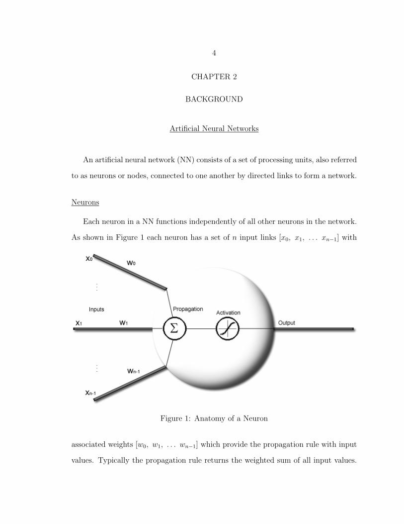
Each neuron in a NN functions independently of all other neurons in the network.
As shown in Figure 1 each neuron has a set of n input links [x0, x1, . . . xn−1] with
Figure 1: Anatomy of a Neuron
associated weights [w0, w1, . . . wn−1] which provide the propagation rule with input
values. Typically the propagation rule returns the weighted sum of all input values.
5
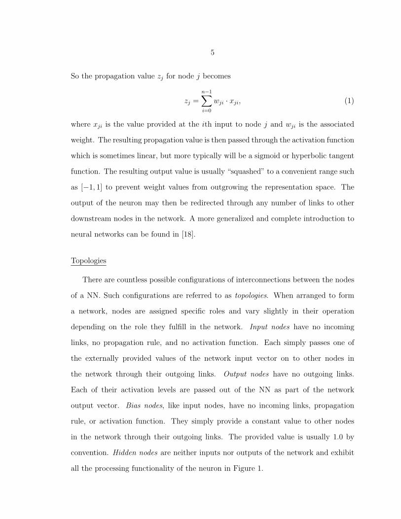
So the propagation value zj for node j becomes
zj =n−1∑i=0
wji · xji, (1)
where xji is the value provided at the ith input to node j and wji is the associated
weight. The resulting propagation value is then passed through the activation function
which is sometimes linear, but more typically will be a sigmoid or hyperbolic tangent
function. The resulting output value is usually “squashed” to a convenient range such
as [−1, 1] to prevent weight values from outgrowing the representation space. The
output of the neuron may then be redirected through any number of links to other
downstream nodes in the network. A more generalized and complete introduction to
neural networks can be found in [18].
Topologies
There are countless possible configurations of interconnections between the nodes
of a NN. Such configurations are referred to as topologies. When arranged to form
a network, nodes are assigned specific roles and vary slightly in their operation
depending on the role they fulfill in the network. Input nodes have no incoming
links, no propagation rule, and no activation function. Each simply passes one of
the externally provided values of the network input vector on to other nodes in
the network through their outgoing links. Output nodes have no outgoing links.
Each of their activation levels are passed out of the NN as part of the network
output vector. Bias nodes, like input nodes, have no incoming links, propagation
rule, or activation function. They simply provide a constant value to other nodes
in the network through their outgoing links. The provided value is usually 1.0 by
convention. Hidden nodes are neither inputs nor outputs of the network and exhibit
all the processing functionality of the neuron in Figure 1.
6
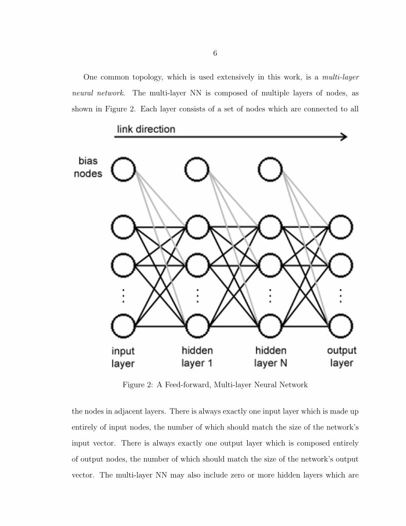
One common topology, which is used extensively in this work, is a multi-layer
neural network. The multi-layer NN is composed of multiple layers of nodes, as
shown in Figure 2. Each layer consists of a set of nodes which are connected to all
Figure 2: A Feed-forward, Multi-layer Neural Network
the nodes in adjacent layers. There is always exactly one input layer which is made up
entirely of input nodes, the number of which should match the size of the network’s
input vector. There is always exactly one output layer which is composed entirely
of output nodes, the number of which should match the size of the network’s output
vector. The multi-layer NN may also include zero or more hidden layers which are

7
made up of hidden nodes, the number of which may be arbitrary and vary among
layers. Typically a bias node will be connected to each node in the hidden and output
layers. Sometimes there is one bias node per layer for convenience of implementation.
Either arrangement is equivalent.
In a feed-forward network like the one pictured in Figure 2, all links are directed
downstream. In the fully-connected variant, nodes connect not only to the adjacent
downstream layer, but also to all nodes in all downstream layers. An example fully-
connected, feed-forward, multi-layer NN is pictured in Figure 3.
Figure 3: An Example of a Fully-connected, Feed-forward, Multi-layer NeuralNetwork
8
Learning Algorithms
In order for a neural network to perform useful computation, it generally needs
to be trained. Training consists of setting the link weights to values appropriate to
the desired computation. This is often done through an iterative process known as a
learning algorithm.
There are numerous learning algorithms for neural networks, often they are tied
closely to the network structure. Common algorithms for the types of networks used
in this work include backpropagation and evolution.
Backpropagation
Backpropagation is a supervised learning method introduced by Paul Werbos in
his 1974 Harvard doctoral thesis[19]. This method is particularly simple to implement
for feed-forward neural networks but can be adapted to handle recurrent structures
as well[20].
Backpropagation works by computing the effective error at each node in the
network given a set of test input vectors [~i0, ~i1, . . . ~in] with corresponding target
output vectors [~t0, ~t1, . . . ~tn]. The weights on each node’s incoming links can then
be adjusted proportionally to reduce the error. Over the course of many iterations,
the error can be minimized, resulting in correct outputs, even for inputs not included
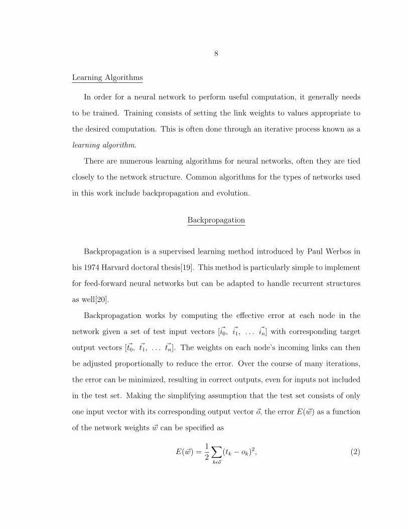
in the test set. Making the simplifying assumption that the test set consists of only
one input vector with its corresponding output vector ~o, the error E(~w) as a function
of the network weights ~w can be specified as
E(~w) =1
2
∑kε~o
(tk − ok)2, (2)
9
where ~t is the target output specified by the test set. The error term δj for node j
can then be defined as
δj =∂E(~w)
∂zj. (3)
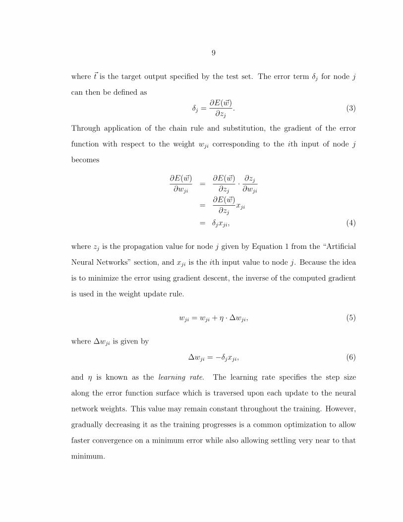
Through application of the chain rule and substitution, the gradient of the error
function with respect to the weight wji corresponding to the ith input of node j
becomes
∂E(~w)
∂wji=
∂E(~w)
∂zj· ∂zj∂wji
=∂E(~w)
∂zjxji
= δjxji, (4)
where zj is the propagation value for node j given by Equation 1 from the “Artificial
Neural Networks” section, and xji is the ith input value to node j. Because the idea
is to minimize the error using gradient descent, the inverse of the computed gradient
is used in the weight update rule.
wji = wji + η ·∆wji, (5)
where ∆wji is given by
∆wji = −δjxji, (6)
and η is known as the learning rate. The learning rate specifies the step size
along the error function surface which is traversed upon each update to the neural
network weights. This value may remain constant throughout the training. However,
gradually decreasing it as the training progresses is a common optimization to allow
faster convergence on a minimum error while also allowing settling very near to that
minimum.
10
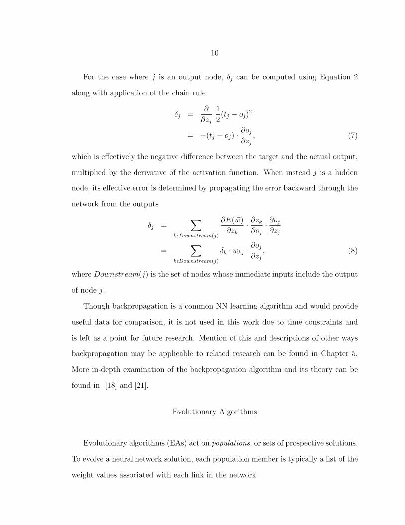
For the case where j is an output node, δj can be computed using Equation 2
along with application of the chain rule
δj =∂
∂zj
1
2(tj − oj)2
= −(tj − oj) ·∂oj∂zj
, (7)
which is effectively the negative difference between the target and the actual output,
multiplied by the derivative of the activation function. When instead j is a hidden
node, its effective error is determined by propagating the error backward through the
network from the outputs
δj =∑
kεDownstream(j)
∂E(~w)
∂zk· ∂zk∂oj· ∂oj∂zj
=∑
kεDownstream(j)
δk · wkj ·∂oj∂zj
, (8)
where Downstream(j) is the set of nodes whose immediate inputs include the output
of node j.
Though backpropagation is a common NN learning algorithm and would provide
useful data for comparison, it is not used in this work due to time constraints and
is left as a point for future research. Mention of this and descriptions of other ways
backpropagation may be applicable to related research can be found in Chapter 5.
More in-depth examination of the backpropagation algorithm and its theory can be
found in [18] and [21].
Evolutionary Algorithms
Evolutionary algorithms (EAs) act on populations, or sets of prospective solutions.
To evolve a neural network solution, each population member is typically a list of the
weight values associated with each link in the network.
11
The initial population members are randomly generated with reasonable values
for the problem space. Each iteration of the EA is called a generation because at the
end of each one, all the populations have been replaced by their successors.
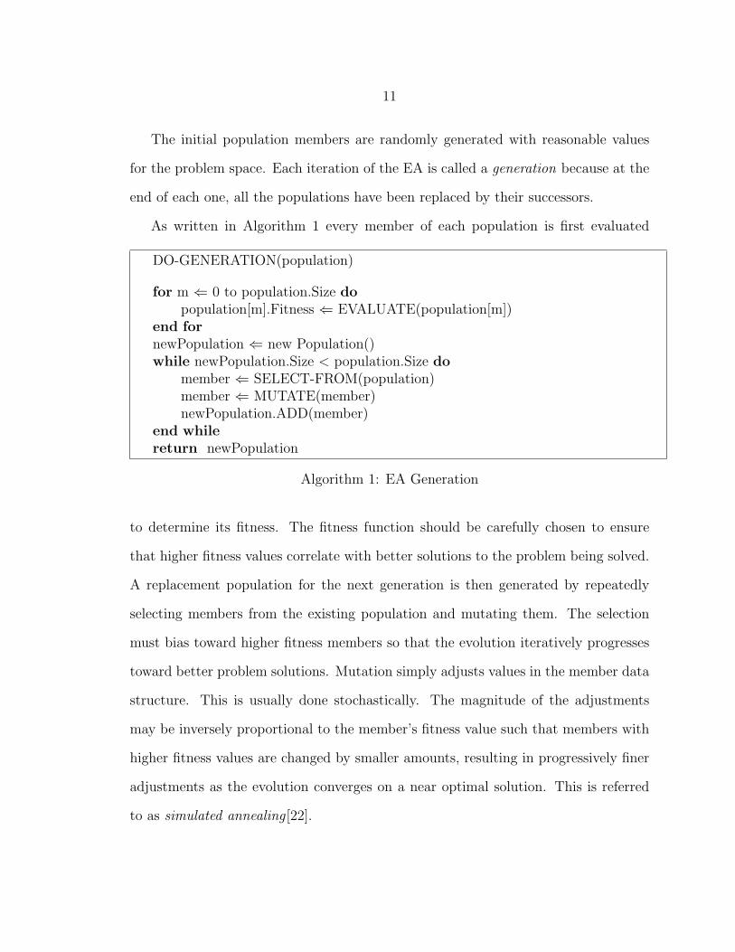
As written in Algorithm 1 every member of each population is first evaluated
DO-GENERATION(population)
for m ⇐ 0 to population.Size dopopulation[m].Fitness ⇐ EVALUATE(population[m])
end fornewPopulation ⇐ new Population()while newPopulation.Size < population.Size do
member ⇐ SELECT-FROM(population)member ⇐ MUTATE(member)newPopulation.ADD(member)
end whilereturn newPopulation
Algorithm 1: EA Generation
to determine its fitness. The fitness function should be carefully chosen to ensure
that higher fitness values correlate with better solutions to the problem being solved.
A replacement population for the next generation is then generated by repeatedly
selecting members from the existing population and mutating them. The selection
must bias toward higher fitness members so that the evolution iteratively progresses
toward better problem solutions. Mutation simply adjusts values in the member data
structure. This is usually done stochastically. The magnitude of the adjustments
may be inversely proportional to the member’s fitness value such that members with
higher fitness values are changed by smaller amounts, resulting in progressively finer
adjustments as the evolution converges on a near optimal solution. This is referred
to as simulated annealing [22].
12
Each generation is completed by replacing all the populations in this way. The
EA continues running one generation after another until a stopping condition is
reached. The stopping condition might be to end after completing a fixed number of
generations, or to end when a particular fitness value is reached.
Numerous enhancing features may be added to the basic evolutionary algorithm
construction to aid in faster or otherwise improved convergence[23]. When the top
n most fit population members are preserved un-mutated between generations, those
members are referred to as elite members. When the fitness function has no stochastic
components, elitism[24] provides a monotonic increase in the peak fitness value from
one generation to the next.
Genetic Algorithms
Though genetic algorithms (GAs) and EAs have developed separately from
one another, their basic operation varies little. The most significant difference
between them is the inclusion of a crossover operation in the GA during replacement
population creation. The crossover operator combines features from two parent
population members to produce either one or two (depending on the implementation)
child members for the next generation. The children are then mutated as usual.
The addition of crossover is illustrated by Algorithm 2 which is otherwise the same
as Algorithm 1. Instead of selecting a single member and mutating it, two members
are selected, producing the child to be mutated and added to the replacement
population.
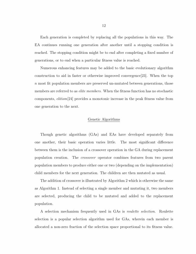
A selection mechanism frequently used in GAs is roulette selection. Roulette
selection is a popular selection algorithm used for GAs, wherein each member is
allocated a non-zero fraction of the selection space proportional to its fitness value.

13
DO-GENERATION(population)
for m ⇐ 0 to population.Size dopopulation[m].Fitness ⇐ EVALUATE(population[m])
end fornewPopulation ⇐ new Population()while newPopulation.Size < population.Size do
mother ⇐ SELECT-FROM(population)father ⇐ SELECT-FROM(population)child ⇐ CROSSOVER(mother, father)child ⇐ MUTATE(child)newPopulation.ADD(child)
end whilereturn newPopulation
Algorithm 2: GA Generation
Figure 4 illustrates this concept with a circular selection space where each member’s
allocated fraction is represented by the arc length for its associated sector. The
selection point is then chosen at random, uniformly within the selection space. In
the circular space shown in Figure 4 the selection point is simply a real valued angle
x such that 0◦ ≤ x < 180◦. The member associated with the fraction of selection
space containing the selection point is returned as the selected member. The highest
fitness individuals occupy more of the selection space and are therefore more likely to
be chosen than low fitness individuals, yet selection of low fitness individuals remains
possible.
The crossover operator combines values from both parent solutions and, like
mutation, often includes a stochastic component. An example crossover operation
for value lists (such as lists of NN weights) is shown in Figure 5. The values to
the left of the crossover point are copied from the first parent and values to the
right of the crossover point are copied from the second parent. This method of
data combination from two parents is referred to as single point crossover. Mitchell,
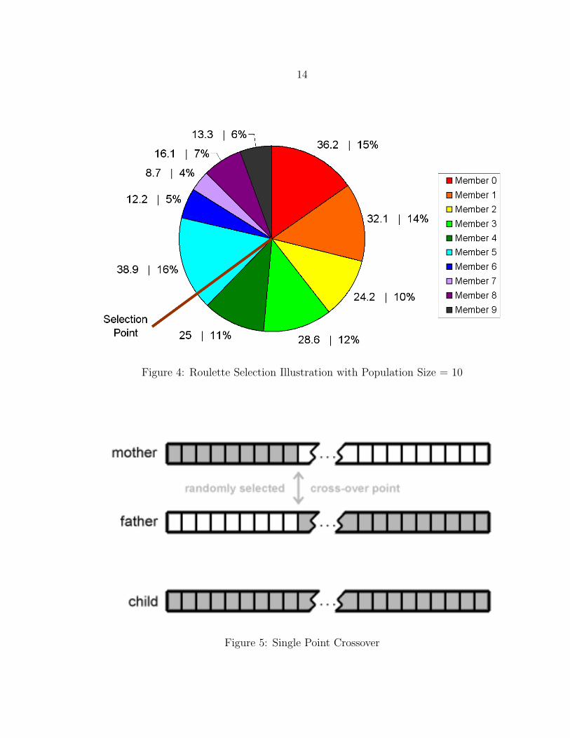
14
Figure 4: Roulette Selection Illustration with Population Size = 10
Figure 5: Single Point Crossover
15
Forest, and Holland[25] showed that GAs with crossover can converge upon high
fitness solutions significantly faster than GAs without crossover.
GNARL
Angeline, Saunders, and Pollack developed an EA specifically for evolving neural
network topologies. In the words of the authors:
“GNARL, which stands for GeNeralized Acquisition of Recurrent Links,is an evolutionary algorithm that nonmonotonically constructs recurrentnetworks to solve a given task. The name GNARL reflects the typesof networks that arise from a generalized network induction algorithmperforming both structural and parametric learning. Instead of havinguniform or symmetric topologies, the resulting networks have ‘gnarled’interconnections of hidden units which more accurately reflect constraintsinherent in the task.”
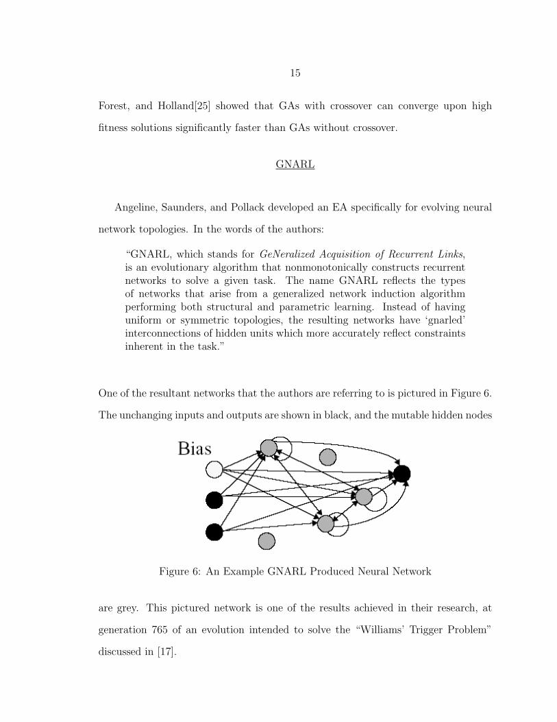
One of the resultant networks that the authors are referring to is pictured in Figure 6.
The unchanging inputs and outputs are shown in black, and the mutable hidden nodes
Figure 6: An Example GNARL Produced Neural Network
are grey. This pictured network is one of the results achieved in their research, at
generation 765 of an evolution intended to solve the “Williams’ Trigger Problem”
discussed in [17].
16
Due to an interest in exploring evolved topologies as well as parametric evolution,
the evolutionary approach to neural networks taken in this work was based upon
GNARL[17].
The inputs and outputs of a GNARL evolved neural network are fixed by the
problem being solved and cannot be changed by the algorithm. Links may be placed
between any two nodes with a few restrictions:
R1: There can be no links to an input node.
R2: There can be no links from an output node.
R3: Given two nodes x and y, there is at most one link from x to y.
Initialization
Initial networks are generated with a random number of hidden nodes and a
random number of links. Both numbers are selected from a uniform distribution
within supplied ranges. The incident nodes for all links are chosen randomly from
possibilities that satisfy the restrictions given above. All link weights are assigned
random values selected uniformly from the range [−1, 1].
Selection
Networks scoring in the top 50% of the population by fitness survive to become
parents of the next generation. The lower 50% are discarded. The replacement
population for each generation is composed of mutated copies of the surviving
members of the previous generation.
17
Mutation
Two types of mutation may be performed. Parametric mutations are adjustments
to weight values. Parametric mutations do not alter network structure. Structural
mutations are changes to the number or relative placement of nodes and links in the
network. For both types, the severity of mutation for a given population member m
is dictated by its temperature T (m) as given by Equation 9:
T (m) = 1− f(m)
fmax, (9)
where fmax is the maximum fitness for the problem being solved. The mutation
severity adjustment has the effect of simulated annealing on the evolution, allowing
for a coarse grained search initially and proceeding to a finer-grained search as the
algorithm converges on a solution.
GNARL also uses an instantaneous temperature T which helps avoid parametric
local minima during the search:
T (m) = U(0, 1)T (m), (10)
where U(a, b) is a uniform random variable in the range [a, b], and in this case [0, 1].
In effect the instantaneous temperature allows for a low frequency occurrence of large
mutations.
Parametric Mutation: Parametric mutations are performed by perturbing each
value with Gaussian noise. For a link weight w the adjustment would be:
∆w = N(0, αT (m)), (11)
where α is a user-defined proportionality constant, and N(µ, σ2) is a Gaussian random
variable with mean µ and variance σ2.
18
Structural Mutation: Structural mutations alter the number of nodes and/or
links in the network. All structural mutations strive to preserve neural network
behavior. Accordingly, nodes are added without any initial links and new links are
added with weights of zero. Such preservation is usually impossible when removing
nodes and links. Removing a node involves the removal of all incident links as well,
which can significantly affect network behavior. When a link is removed, the nodes it
connects are not and may be left with no connections. Future mutations may remove
the floating node, or reconnect it.
The number of additions or deletions ∆ for both nodes and links is restricted to a
user defined range [∆min,∆max]. The range is defined independently for each of the
four structural mutation types. Selection of ∆ from the available range for a given
mutation type depends upon the individual’s instantaneous temperature:
∆ = ∆min + bU [0, 1]T (m)(∆max −∆min)c. (12)
Selection of a node for removal is uniform across all nodes excepting inputs and
outputs. Similarly, selection of a link for removal is uniform across all links in the
network. Adding a link involves another parameter specifying the probability that
each endpoint will be selected from the network input and output nodes instead
of from the bias and hidden nodes. Every time the selection of a link endpoint is
required, a node class selection is made according to the specified probability. A
node is then chosen uniformly from the selected class to become the link’s endpoint.
Fractional Order Calculus
Fractional order calculus has remained a topic of scholarly interest since the
beginning of differential calculus. As is frequently noted, Leibniz and L’Hopital

19
corresponded on the subject as early as 1695[26, 27]. Over the past 30 years it has
received increased interest in its applications. Numerous recent applications in the
field of control theory[14, 28] have been successful. Gorenflo and Mainardi[26] aptly
describe it as “. . . the field of mathematical analysis which deals with the investigation
and applications of integrals and derivatives of arbitrary order.”
The definition of the differintegral upon which this work is based depends on the
Gamma function as given in Equation 13
Γ(z) =
∫ ∞0
tz−1e−t dt, (13)
which for this usage can be succinctly explained as an extension of the better known
factorial function given in Equation 14, to real and complex numbers.
x! =x∏i=1
i (14)
This definition of the differintegral is one first presented by Grunwald and later
extended by Post. As taken from the text by Oldham and Spanier[27]:
dqf
[d(t− a)]q= lim
N→∞
{[t−aN
]−qΓ(−q)
N−1∑k=0
Γ(k − q)Γ(k + 1)
f
(t− k
[t− aN
])}(15)
Collecting the gamma terms and performing the substitution given by Equation 16
ωk =Γ(k − q)
Γ(−q)Γ(k + 1), (16)
yields the formula used in this work to implement the numerical evaluation of the qth
order differintegral of function f between the limits a and t for t > a.
aDqt f(t) = lim
N→∞
{[t− aN
]−q N−1∑k=0
ωk · f(t− k
[t− aN
])}, (17)
where ωk is the kth differintegral weight, N is the number of divisions evaluated
between the limits and the size of the infinitesimal dt is accordingly
dt =t− aN
. (18)
20
Positive orders of differintegration q correspond to derivatives, and negative values of
q correspond to integrals. The case where q = 1.0 reduces to the well known definition
of the first derivative of function f at point t given in Equation 19.
df(t)
dt= lim
h→0
f(t)− f(t− h)
h(19)
Similarly, the case where q = −1.0 reduces to a familiar Riemann integral based
definition of the first integral of function f between the limits a and t for t > a given
in Equation 20 ∫ t
a
f(t) = limh→0
hN−1∑i=0
f(t− ih), (20)
where N = t−ah
.
It is interesting to consider the differintegral weight values ωk for specific values
of q. A simple recursive relationship for computing them can be derived from
Equation 16 using the properties of the gamma function given in Equation 21.
Γ(n+ 1) = nΓ(n) = n!, for n ε Z (21)
Using these properties, it can be shown that ω0 = 1 for all values of q. Substitution
of k = k + 1 into Equation 16 also reveals that
ωk = ωk−1 ·k − 1− q
k. (22)
When q = 1.0, ω0 = 1 and ω1 = −1. All other weights are zero in this case.
This agrees with the simple difference operation applied in Equation 19. Similarly,
when q = −1.0, ω1 and all other weights are equal to 1. This agrees with the
simple summing behavior demonstrated in Equation 20. Results are similar with
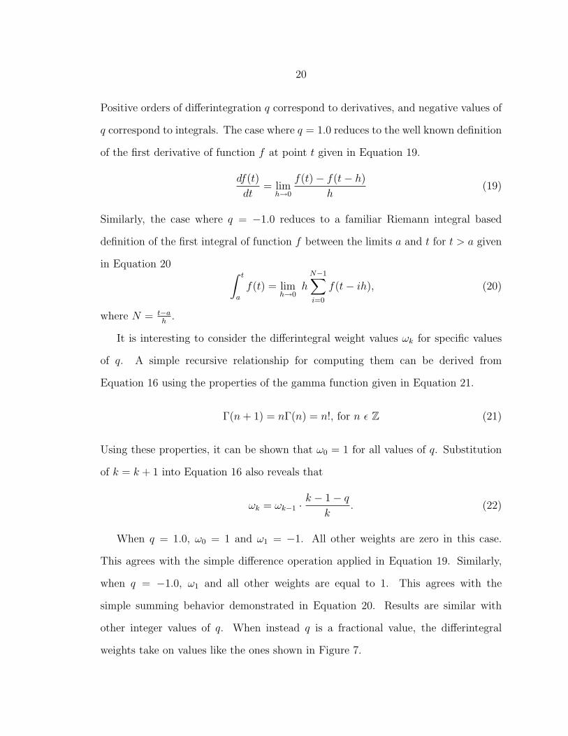
other integer values of q. When instead q is a fractional value, the differintegral
weights take on values like the ones shown in Figure 7.
21
(a) q = 0.5
(b) q = −0.5
Figure 7: Fractional Order Differintegral Weight Values
22
CHAPTER 3
SYSTEM DESCRIPTION
All experimental results for this project were obtained using a custom software
solution developed specifically for this work. The software itself is described in
detail in Appendix A, along with images of the graphical user interface (GUI) in
operation. Selections from the source code are available in Appendix B. This chapter
describes the differences between the system’s implementation and the background
theory discussed in Chapter 2.
Neural Network Implementation
The neural network implementation used allowed for any number of nodes to be
connected in virtually any configuration. Links to input nodes were ignored and any
non-input node with no inputs was implicitly a bias node. Aside from the mentioned
constraints, links could be made between any two nodes whether the result be forward,
backward, repeated, symmetric, or otherwise. This implementation scheme resulted
in maximum flexibility in running experiments, though very few experiments strayed
from the fully-connected feed-forward topology.
Discrete Differintegral Computation
To apply the differintegral operation shown in Equation 17 to neural networks,
a method based upon the G1-algorithm as described by Bohannan[11] was applied.
The method makes use of a recursive multiplication-addition scheme for computing
the weights of the differintegral while applying them to the input function. The

23
same recursion was used for weight computation in this work, and is described by
Equation 22, from the “Fractional Order Calculus” section of Chapter 2. For this
work, the weights were computed as needed and stored for reuse at each differintegral
computation.
Algorithm 3 shows the method used to compute the weights, where weights is
a dynamic array of differintegral weights (ω0, ω1, . . . ωn) and q is the order of the
differintegral to which the weights apply.
COMPUTE-NEXT-WEIGHT(weights, q)
k ⇐ weights.size()if k = 0 then
weights.add(1.0)else
weights.add(weights[k - 1] * (k - 1 - q) / k)end ifreturn weights
Algorithm 3: Discrete Differintegral Weight Computation
The order q discrete differintegral for the function f(t) over the range [0, t] was
computed using the convolution demonstrated by Algorithm 4, where f is an array
DIFFERINTEGRAL(f, weights, q, dt)
sum ⇐ 0.0N ⇐ f.size()for i ⇐ 0 to N - 1 do
index ⇐ N - 1 - isum ⇐ sum + f[index] * weights[i]
end forreturn sum / pow(dt, q)
Algorithm 4: Differintegral
holding N samples of the function f(t) taken at intervals of size dt, and weights is an
array holding at least the first N weights as computed by Algorithm 3. Algorithm 4

24
makes the simplifying assumption that a mechanism is in place to ensure all necessary
weights are computed and available. Such a mechanism was implemented in the
software used for this work.
Due to the finite nature of computer memory an approximation may be required
to make computation of the differintegral practical over lengthy simulations. The
software implementation used in this work was capable of applying four different
approximation methods. Each resulted in a restriction of the sample history to a
fixed maximum length. The approximation method considered to most closely match
the results using a perfect sample history was referred to as ratio approximation. This
method worked as shown in Algorithm 5, where value is the next sample to be added
ADD-SAMPLE(value, f, weights, L)
if f.size() ≥ L thenratio ⇐ weights[L - 1] / weights[L - 2]discard ⇐ f[0]f.remove(0)f[0] ⇐ discard * ratio
end iff.add(value)return f
Algorithm 5: Ratio Approximation
to the sample history f , weights is the array containing at least the first L weights
computed by Algorithm 3, and L is the maximum sample history length. The oldest
sample f [0] is scaled by the ratio of the smallest weights used in the differintegral.
The result is then added to the next oldest sample f [1]. The oldest sample f [0] is
then discarded to make room for the new value at the end of the sample history.
Most of the experiments performed for this work were short enough to allow
practical computation over the entire sample history and for all those experiments
25
presented in Chapter 4, no approximation was applied. Instead perfect memory of
the sample space was maintained throughout each simulation.
Fractional Calculus Neuron Augmentation
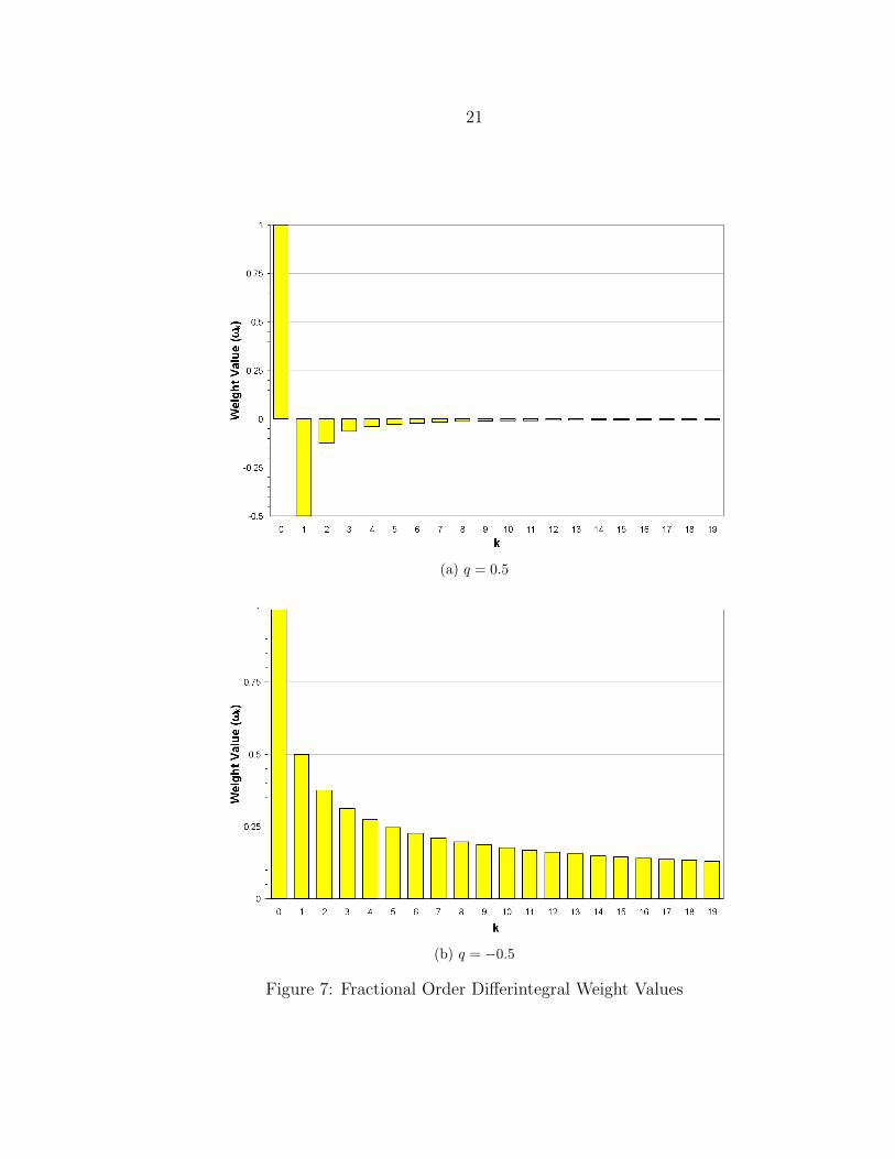
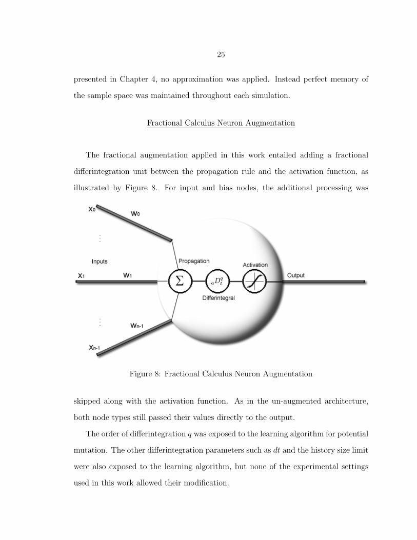
The fractional augmentation applied in this work entailed adding a fractional
differintegration unit between the propagation rule and the activation function, as
illustrated by Figure 8. For input and bias nodes, the additional processing was
Figure 8: Fractional Calculus Neuron Augmentation
skipped along with the activation function. As in the un-augmented architecture,
both node types still passed their values directly to the output.
The order of differintegration q was exposed to the learning algorithm for potential
mutation. The other differintegration parameters such as dt and the history size limit
were also exposed to the learning algorithm, but none of the experimental settings
used in this work allowed their modification.
26
Learning Algorithm
Most of the experiments described in Chapter 4 were performed using fixed
topologies. Learning was achieved by modification of network weights and q values.
This was done primarily to simplify experiments. Some exploration using evolved
topology types was desired however, so to accommodate such experiments a learning
algorithm based on the GNARL algorithm described in Chapter 2 was adopted. Most
of the changes made consisted of adapting rules of operation into adjustable options.
The software was designed to function exactly as described by Angeline, Saunders
and Pollack when configured with the appropriate settings.
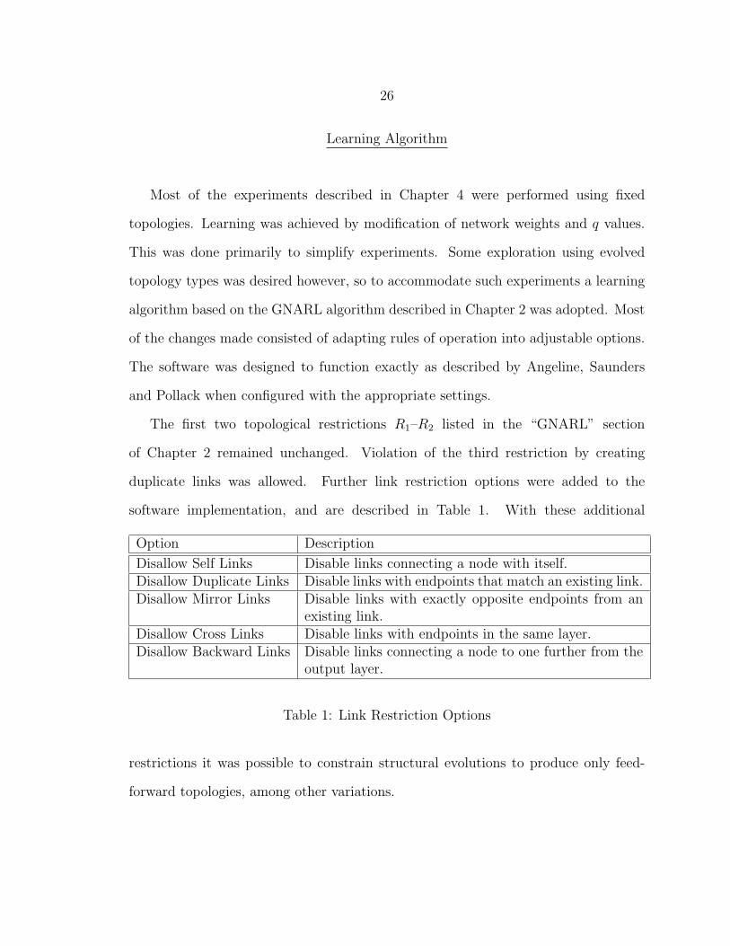
The first two topological restrictions R1–R2 listed in the “GNARL” section
of Chapter 2 remained unchanged. Violation of the third restriction by creating
duplicate links was allowed. Further link restriction options were added to the
software implementation, and are described in Table 1. With these additional
Option Description
Disallow Self Links Disable links connecting a node with itself.Disallow Duplicate Links Disable links with endpoints that match an existing link.Disallow Mirror Links Disable links with exactly opposite endpoints from an
existing link.Disallow Cross Links Disable links with endpoints in the same layer.Disallow Backward Links Disable links connecting a node to one further from the
output layer.
Table 1: Link Restriction Options
restrictions it was possible to constrain structural evolutions to produce only feed-
forward topologies, among other variations.
27
Initialization
Initialization could be defined by the problem space, population member type, or
population type, depending on preference. For the fox/rabbit problem used in this
work, initialization options were provided by the neural network. Several predefined
topologies were available, as well as the random topology used by GNARL. The
weights could be initialized from either a uniform or a Gaussian distribution. The
range of initial values was adjustable.
Selection
The software implementation allowed for the population survival rate between
generations to be altered from the top 50% to any other valid quantity for a
given population size. Any fraction of the population could be designated as elite,
or refreshed. Refreshed members were freshly initialized members added to the
population during each generation in place of mutated members from the previous
generation. The software also implemented some GA-like selection mechanisms
including roulette selection as described in the “Genetic Algorithms” section of
Chapter 2.
Crossover
A crossover operation was also implemented to allow the possibility of configuring
the software as a GA. This was a multi-point crossover algorithm generalized to
allow crossover to occur between parents with varying network topologies. The
operator essentially treated each network as a list of its mutable components. A
parental selection was made for every component in the list to determine which
parent the child’s component would be inherited from. Each parent was assigned

28
equal probability in the selection. In effect this allowed for [0, N−1] crossover points,
where N was the length of the mutable component list.
To allow for varying topologies, the different component types were handled
as sublists. The actual implementation is given in the “Fox/Rabbit Evolutionary
Algorithm Code” section of Appendix B.
Mutation
An option was provided to disable the effect of the temperature value of
Equation 10 from the “GNARL” section of Chapter 2. Instead, a fixed probability
of mutation could be specified, making the evolution behave like a GA. The software
implementation also added options to toggle mutation of all the available parameters
and structural adjustments.
Parametric Mutation: The GNARL algorithm adjusted only network weights.
The software implementation for this work added several other options to the list
of mutable parameters. These are listed in Table 2. Node values were important
Parameter Description
Weights Network link weights.Node Values Network node values.Activation Functions Network node activation function types.Activation Slopes Network node activation function slopes or binary
thresholds.Activation Limits Network node activation function upper and lower
output limits.q Fractional unit orders of differintegration.dt Fractional unit sample rates.History Size Limits Fractional unit maximum sample history lengths.Approximation Methods Fractional unit sample history approximation methods.
Table 2: Mutable Parameter Types
29
because they fully specified the output of bias nodes, as well as providing an initial
value for hidden nodes in recurrent networks to be used while unwrapping loops. An
additional option was provided to force all bias nodes to a constant value. This was
used to maintain bias values of 1.0 for the experiments in this work.
Although none of the experiments performed for this work allowed parametric
mutation of the activation function parameters, options were provided to allow them
to mutate. Activation function choices available were: binary threshold, linear,
sigmoid, and hyperbolic tangent. Each of these functions imposed upper and lower
limits on their output values whether they were attainable (as for binary threshold
and linear units) or asymptotic (as for sigmoid and hyperbolic tangent units). The
slope of the function between the limits was also adjustable where applicable. In the
case of the binary threshold function, the slope parameter was used to specify the
cutoff threshold determining which limit was output by the function.
The only parameter related to the fractional units that was allowed to mutate for
the experiments described in Chapter 4 was q. Other mutable parameters included the
sample rate dt and the maximum sample history length. The available sample history
approximation functions used in limiting the sample history length were: truncation,
coopmans, exponential, and ratio. Truncation took no pains to avoid ringing and
other signal artifacts related to abruptly forgetting sample values. Coopmans followed
the algorithm of the same name, in adding the lost values to the beginning of the
sample history. Exponential used a fixed decay of 0.99 applied to lost values before
adding them to the end of the sample history, which was nearly the same as the ratio
approximation described in the “Discrete Differintegral Computation” section.
Structural Mutation: The GNARL algorithm allows for addition and removal
of links during network evolution. The software implementation used in this work
30
added an ability to change the type of network nodes. The only types available for
this work were un-augmented neurons, and fractionally augmented neurons. The
mechanism for changing node types was identical to that for adding or removing
nodes, with specified range [∆min,∆max] for the number of changes ∆ made during
each mutation. The selection of ∆ was made based on the instantaneous temperature,
using Equation 12 from the “GNARL” section of Chapter 2.
Other changes to structural mutation included the additional link restriction
options given in Table 1 and an option to add exactly one input link and one output
link with each new node, ensuring that it would be connected to the rest of the
network.
Statistic Collection
For each evolution run by the software implementation, basic fitness statistics
were aggregated across all members in a population, across all populations in the EA,
and then across all generations run by the EA. These provided information such as
the maximum fitness in each population at the end of any given generation, or the
maximum fitness achieved by any population throughout the entire evolution.
Problem specific statistics were also collected at each of these levels, and each
problem could define additional levels for statistic collection. In the case of the
artificial life simulation described in Chapter 4, these included things like distance
between entities, and the speed of the fox at any given time step. The time-step-
level statistics were aggregated across all time steps in the simulation before joining
simulation-level statistics to be aggregated across all simulation trials for each member
evaluation. These results were then joined with member level statistics to be further
aggregated alongside the fitness values.
31
CHAPTER 4
EXPERIMENTS AND RESULTS
Several experiments were run utilizing an artificial life simulation to compare the
un-augmented neural network (NN) to the fractionally augmented neural network
(FNN).
Artificial Life Simulation
The simulation took place on a 2-dimensional (2D) bounded field. Two virtual
creatures were placed within the bounds of the field along with optional obstacles,
depending on the experiment. All entities in the simulation were circular and fully
specified by a 2D position coordinate and a radius. Creatures were allowed to move
by changing their acceleration vectors which indirectly affected their velocity vectors.
They were not allowed to pass through the walls (field boundaries) or obstacles on
the field. One of these creatures was designated as the “fox” and the other as the
“rabbit”. The rabbit’s goal was to evade the fox until the simulation’s end. The fox’s
goal was to capture the rabbit by touching or passing through it at some point during
the simulation.
The rabbit’s movement was dictated by simulation settings which varied by
experiment. The movement of the fox was dictated by the outputs of a controlling
neural network. The two outputs formed a 2D acceleration vector with coordinate
values in the range [−1, 1]. These were scaled to the the range of the maximum
acceleration magnitude and applied to the fox’s movement at each simulation time
step. The inputs to the neural network were generated by a virtual sensor array. Each
32
sensor in the array provided two values to the fox’s neural network, one indicating the
average entity type sensed and another indicating the average intensity (or closeness)
of entities sensed.
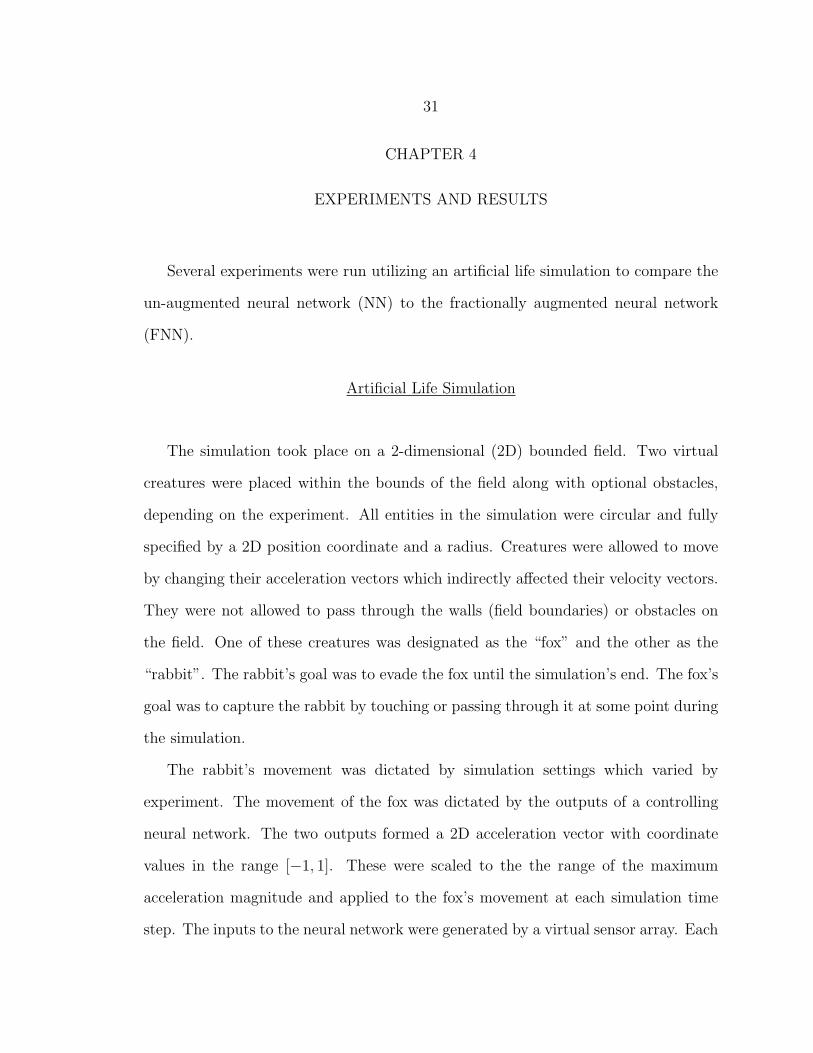
The number of sensors was variable and dictated by simulation settings. As
illustrated in Figure 9, the 360◦ around the fox was divided evenly into sensor sectors
Figure 9: Fox Sensor Array
starting from 0◦. The sensor array did not rotate with the fox’s movement, so the
boundary between the first and last sensors always pointed in the direction of the
positive X-axis. Each sensor was further divided into a number of equal sub-sectors,
or cells, specified by an alterable resolution setting. The real valued type and intensity
for each sensor were generated by averaging the type and intensity across its cells.
The type value returned by each cell was determined by the nearest entity in its
sensed range and is given by Table 3. The intensity value returned by each cell was
computed according to Equation 23,

33
Entity ValueWall or Obstacle -1None 0Creature 1
Table 3: Sensor Cell Type Values
intensity = 1− d
dmax, (23)
where d is the distance to the nearest sensed entity and dmax is the maximum possible
separation distance. The value of dmax depended on the dimensions of the field.
The sensor array was planned as described in an effort to provide a large quantity
of sensory input data which included some ambiguity. Use of memory in the FNN
was expected to be beneficial in resolving the ambiguous sensor states. The two layer
sensor/cell scheme provided the added benefit that it required relatively few inputs
to the neural network.
To measure the fox’s performance and to provide neural network fitness values to
the encapsulating evolution, each simulation returned a score. This was a single value
which ideally indicated how close the fox came to accomplishing its goal of capturing
the rabbit. Because of the stochastic nature of the simulation, the actual fitness
values (in the scope of the evolution) were computed by averaging each fox’s score
using a given neural network over several simulation trials. Despite this technicality,
the scoring function may be referred to as the fitness function. The fitness function
could be chosen and modified by simulation settings.
Common Experimental Parameters
The software solution used to run each of the experiments in this work allowed
for the configuration of a large variety of settings. To relieve any possible confusion,
34
the base set of parameters common among the experiments in this work are provided
in this section. Variations on these parameters are described with the experiments
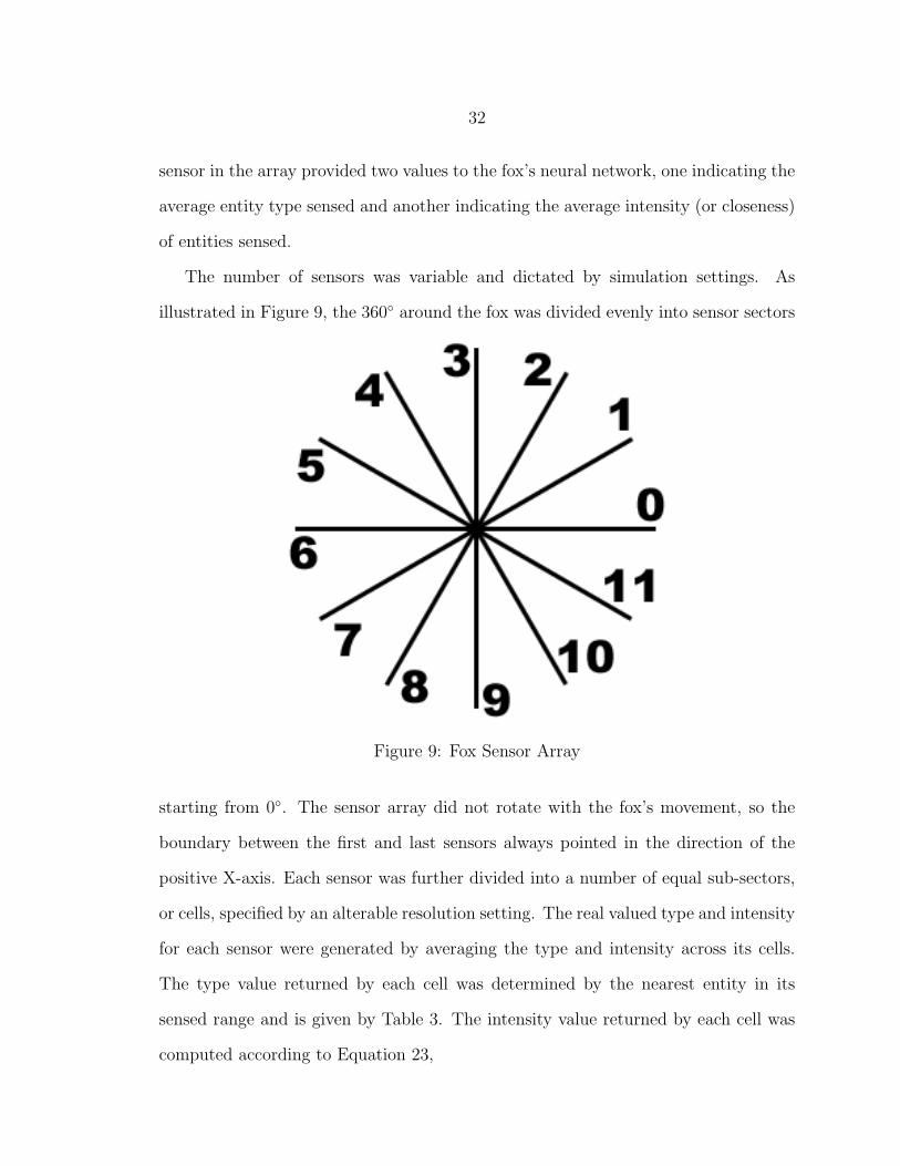
they affect. Table 4 provides all common evolution related parameters while Table 5
Name Value DescriptionPopulation Size 32 Members per population.Elite Members 2 Number of top members maintained as elite. (5%)Generations 1000 Length of the evolution in generations.Trials 10 Simulations run to determine the fitness of each
member.Runs 4 Copies of each experiment run for data collection.
Table 4: Base Experimental Evolution Parameters
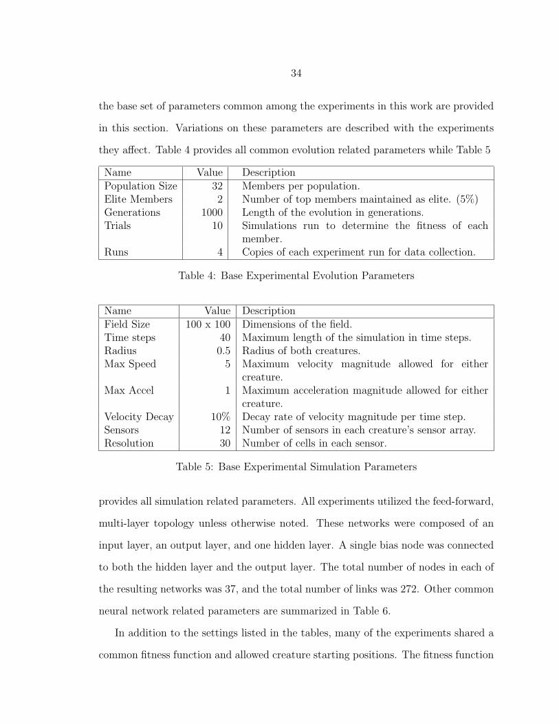
Name Value DescriptionField Size 100 x 100 Dimensions of the field.Time steps 40 Maximum length of the simulation in time steps.Radius 0.5 Radius of both creatures.Max Speed 5 Maximum velocity magnitude allowed for either
creature.Max Accel 1 Maximum acceleration magnitude allowed for either
creature.Velocity Decay 10% Decay rate of velocity magnitude per time step.Sensors 12 Number of sensors in each creature’s sensor array.Resolution 30 Number of cells in each sensor.
Table 5: Base Experimental Simulation Parameters
provides all simulation related parameters. All experiments utilized the feed-forward,
multi-layer topology unless otherwise noted. These networks were composed of an
input layer, an output layer, and one hidden layer. A single bias node was connected
to both the hidden layer and the output layer. The total number of nodes in each of
the resulting networks was 37, and the total number of links was 272. Other common
neural network related parameters are summarized in Table 6.
In addition to the settings listed in the tables, many of the experiments shared a
common fitness function and allowed creature starting positions. The fitness function

35
Name Value DescriptionBias Nodes 1 Number of bias nodes. (value = 1.0)Input Nodes 24 Number of input nodes. (2 per sensor)Hidden Nodes 10 Number of hidden nodes. (1 layer)Output Nodes 2 Number of output nodes.Activation Function Linear Activation function used by network nodes.Activation Slope 1.0 Activation function slope.Activation Max 1.0 Maximum activation function output value.Activation Min -1.0 Minimum activation function output value.Initial Weights N(0, 1.02) Distribution of initial random weight values.Initial Node Values N(0, 1.02) Distribution of initial random node values.Initial Qs N(0, 0.52) Distribution of initial random FNN Q values.History Limit None Maximum FNN sample history length.
Table 6: Base Experimental Neural Network Parameters
applied was referred to as bidirectional-approach and generated values in the range
[0.0, 100.0]. Its value for a given simulation was 100.0 if the fox successfully captured
the rabbit. Otherwise, its value was computed using Equation 24,
Score = 40 + 40 ·∑smax−1
s=0 Approachssmax
(24)
where smax is the maximum number of time steps in the simulation, and Approachs
is given by Equation 25,
Approachs =
1, if d < 0;
0, if d = 0;
−1, if d > 0.
(25)
such that d is the instantaneous derivative of the separating distance between the fox
and rabbit with respect to simulation time.
The rabbit starting position, unless otherwise specified, was at the origin (0,0)
which was located in the center of the field. The fox starting position was at any
randomly chosen point on a circle of radius 49.5 and centered at the origin. This

36
arrangement was such that the fox (having radius = 0.5) would touch the field
boundary if the starting angle happened to place it on either the X or Y-axis.
Baseline
The baseline experiment compared the NN to the FNN using the parameters
detailed in the previous section. This provided a general idea how the performance
of the un-augmented networks and the fractionally augmented networks compared in
the context of one of the simplest experiments possible using the fox/rabbit artificial
life simulation. This experiment also served as a baseline for comparison with other
experiments.
Figure 10 compares plots of the NN and FNN’s maximum fitness values averaged
Figure 10: Baseline – Average Maximum Fitness vs Generation
37
across all four evolutions for each network type. From the plot, the NN’s maximum
fitness curve appears to rise quickly early in the evolution. It then levels off at about
600 generations. The FNN’s maximum fitness looks more linear with some leveling
in the last 100 generations.
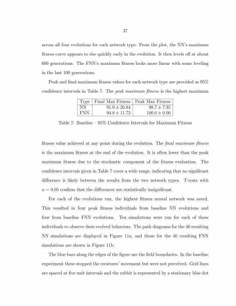
Peak and final maximum fitness values for each network type are provided as 95%
confidence intervals in Table 7. The peak maximum fitness is the highest maximum
Type Final Max Fitness Peak Max FitnessNN 91.9± 26.84 98.7± 7.35FNN 94.8± 11.72 100.0± 0.00
Table 7: Baseline – 95% Confidence Intervals for Maximum Fitness
fitness value achieved at any point during the evolution. The final maximum fitness
is the maximum fitness at the end of the evolution. It is often lower than the peak
maximum fitness due to the stochastic component of the fitness evaluation. The
confidence intervals given in Table 7 cover a wide range, indicating that no significant
difference is likely between the results from the two network types. T-tests with
α = 0.05 confirm that the differences are statistically insignificant.
For each of the evolutions run, the highest fitness neural network was saved.
This resulted in four peak fitness individuals from baseline NN evolutions and
four from baseline FNN evolutions. Ten simulations were run for each of these
individuals to observe their evolved behaviors. The path diagrams for the 40 resulting
NN simulations are displayed in Figure 11a, and those for the 40 resulting FNN
simulations are shown in Figure 11b.
The blue bars along the edges of the figure are the field boundaries. In the baseline
experiment these stopped the creatures’ movement but were not perceived. Grid lines
are spaced at five unit intervals and the rabbit is represented by a stationary blue dot

38
(a) NN (b) FNN
Figure 11: Baseline – Behavior Visualization
in the center of the field. The 40 foxes are represented by warm colored dots (reds,
oranges, and yellows) with matching colored lines showing the paths they followed
from their starting positions in a circle around the rabbit. All 40 simulations are
overlaid in the same field, but no interaction occurred among them.
The area of high path density around the rabbit in Figure 11a is larger than that
of Figure 11b. This is because the NNs exhibit relatively slow and broad, smooth
arcing movement. The FNNs, on the other hand, tend to make more abrupt changes,
though often arcing smoothly as well. This behavioral discrepancy is illustrated more
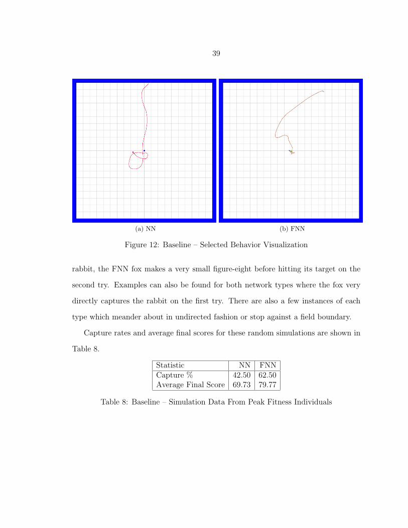
clearly in Figure 12. The NN behavior pictured in Figure 12a is fairly typical in that,
upon missing the rabbit in its first pass, the fox circles back in a large gentle arc to
try again. In this case, it misses a second time, but the second loop is also tighter.
If the simulation were allowed to continue beyond the 40 time step limit, the fox
might have eventually caught the rabbit. In contrast, the FNN behavior displayed
in Figure 12b shows a much tighter turn-around mechanism. Upon first missing the
39
(a) NN (b) FNN
Figure 12: Baseline – Selected Behavior Visualization
rabbit, the FNN fox makes a very small figure-eight before hitting its target on the
second try. Examples can also be found for both network types where the fox very
directly captures the rabbit on the first try. There are also a few instances of each
type which meander about in undirected fashion or stop against a field boundary.
Capture rates and average final scores for these random simulations are shown in
Table 8.
Statistic NN FNNCapture % 42.50 62.50Average Final Score 69.73 79.77
Table 8: Baseline – Simulation Data From Peak Fitness Individuals

40
Non-Resetting
In all other experiments, the foxes’ controlling neural networks were reset between
each simulation trial to clear any state information that may have been stored
in the network. For this non-resetting experiment the networks were allowed to
retain their states from one trial to the next during any given generation. The
feed-forward topology prevents the NNs from holding state information, so only
differences in the FNN were considered. A comparison between the non-resetting
average maximum fitness values and those of the baseline experiment is shown in
Figure 13. No significant differences are evident from the plot. Quantitative analysis
Figure 13: Non-Resetting – Average Maximum Fitness vs Generation
verifies this conclusion. A t-test with α = 0.05 shows that the two plots are
41
statistically equivalent. Peak and final maximum fitness values for both the non-
resetting experiment and the baseline are provided as 95% confidence intervals in
Table 9, for comparison. The overlap between the confidence intervals is even more
convincing that the two results are the same.
Experiment Final Max Fitness Peak Max FitnessNon-Resetting FNN 92.2± 14.31 100.0± 0.00Baseline FNN 94.8± 11.72 100.0± 0.00
Table 9: Non-Resetting – 95% Confidence Intervals for Maximum Fitness
This finding is somewhat surprising because the discontinuity between trials was
expected to leave the networks in inappropriate states at the beginning of each
successive trial. Instead the FNN seems to be adaptable to such inconsistencies.
Hidden Layer Size Comparison
To determine if the size of the hidden layer affected the fitness results for either
the NN or FNN, the baseline test was repeated several times with varying numbers of
hidden nodes in the controlling networks. In addition to the 10 hidden node baseline
experiment, data was collected for 0, 5, 15, and 20 node hidden layers for both the
NN and FNN.
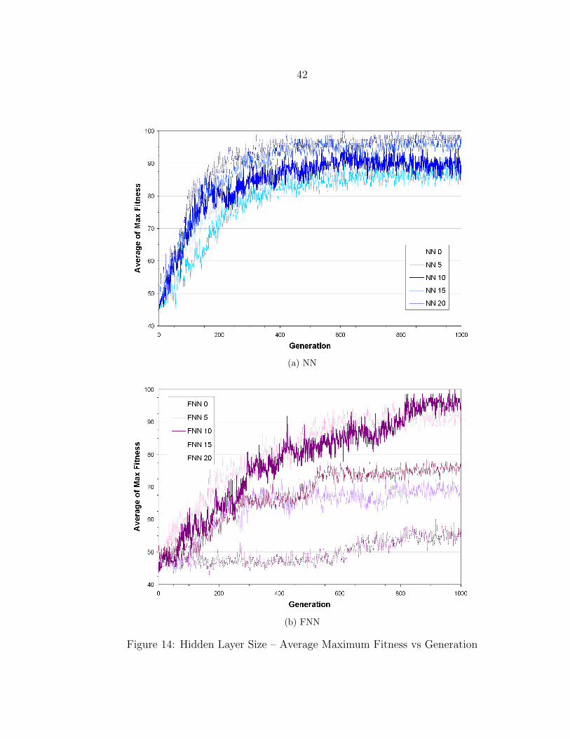
The average maximum fitness values plotted over the entire length of the evolution
are shown in Figure 14. In visually examining the NN plots shown in Figure 14a,
a relationship between the number of hidden nodes and the fitness data appears
evident. With the exception of the zero node case, the plots for networks with higher
numbers of hidden nodes appear higher on the fitness plot. This indicates that the
NN produced higher fitness results with an increase in the number of nodes in the
hidden layer. No direct relationship between the number of hidden nodes and the
42
(a) NN
(b) FNN
Figure 14: Hidden Layer Size – Average Maximum Fitness vs Generation
43
fitness data is apparent in the FNN plots displayed in Figure 14b. There does appear
to be wider variation between the plots, than for the NN data.
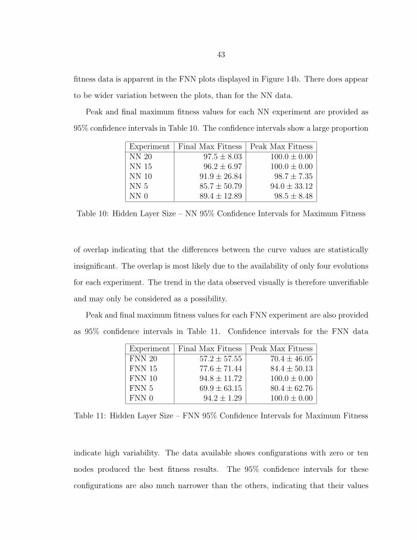
Peak and final maximum fitness values for each NN experiment are provided as
95% confidence intervals in Table 10. The confidence intervals show a large proportion
Experiment Final Max Fitness Peak Max FitnessNN 20 97.5± 8.03 100.0± 0.00NN 15 96.2± 6.97 100.0± 0.00NN 10 91.9± 26.84 98.7± 7.35NN 5 85.7± 50.79 94.0± 33.12NN 0 89.4± 12.89 98.5± 8.48
Table 10: Hidden Layer Size – NN 95% Confidence Intervals for Maximum Fitness
of overlap indicating that the differences between the curve values are statistically
insignificant. The overlap is most likely due to the availability of only four evolutions
for each experiment. The trend in the data observed visually is therefore unverifiable
and may only be considered as a possibility.
Peak and final maximum fitness values for each FNN experiment are also provided
as 95% confidence intervals in Table 11. Confidence intervals for the FNN data
Experiment Final Max Fitness Peak Max FitnessFNN 20 57.2± 57.55 70.4± 46.05FNN 15 77.6± 71.44 84.4± 50.13FNN 10 94.8± 11.72 100.0± 0.00FNN 5 69.9± 63.15 80.4± 62.76FNN 0 94.2± 1.29 100.0± 0.00
Table 11: Hidden Layer Size – FNN 95% Confidence Intervals for Maximum Fitness
indicate high variability. The data available shows configurations with zero or ten
nodes produced the best fitness results. The 95% confidence intervals for these
configurations are also much narrower than the others, indicating that their values
44
are repeatable. Note that when no hidden nodes were present in the network, the
fractional differintegration was still applied in the output nodes.
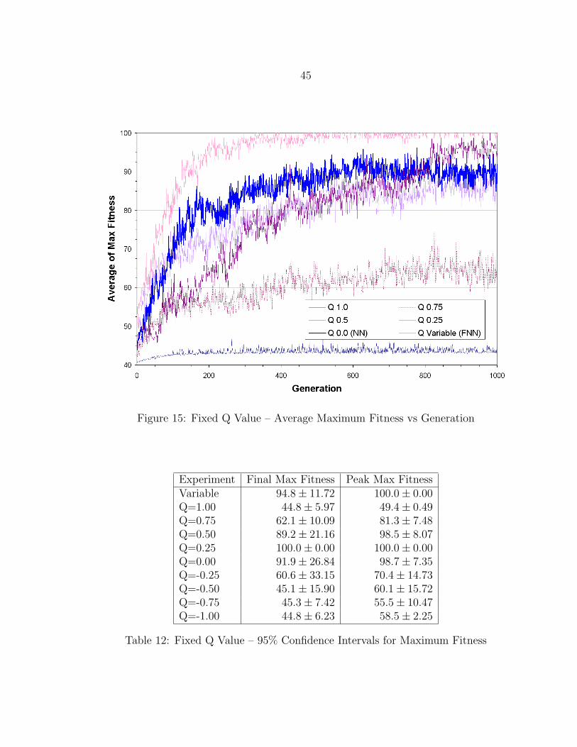
Fixed Q-Value Comparison
To determine whether some orders of differintegration provided better evolution-
ary performance than others, the FNN baseline experiment was run with several
different Q values which were not allowed to mutate during the evolution. Data was
collected for Q values of ±0.25, ±0.5, ±0.75, and ±1.0. The baseline NN experiment
was effectively the same as running an FNN experiment with a fixed Q value of 0.0.
In the case of Q = 1.0 the fractional processing units in each node were performing
simple derivation of their inputs. In the case of Q = −1.0 the fractional processing
units were performing simple accumulation of their inputs.
The experiments using negative Q values all produced plots that looked similar
and provided little information to the observer. Most maintained a maximum fitness
value near 45.0 throughout the evolution. The exception was for Q = −0.25 which
achieved a final fitness value above 55.0. These negative Q value plots are not shown.
The positive Q value average maximum fitness values are plotted in Figure 15, along
with the baseline NN (Q = 0.0) and FNN (Variable) results for comparison. Large
differences in fitness results produced by each fixed Q value experiment are visually
apparent from the plot. The network with Q = 0.25 produced the best result, with the
baseline variable Q data ranking second. The experiments with Q = 0.0 and Q = 0.5
also produced good results. Qualitatively the other experiments produced low fitness
values and can be grouped with the negative Q value experiments as ineffective.
Peak and final maximum fitness values for each fixed Q value experiment are
provided as 95% confidence intervals in Table 12, along with the baseline NN and
45
Figure 15: Fixed Q Value – Average Maximum Fitness vs Generation
Experiment Final Max Fitness Peak Max FitnessVariable 94.8± 11.72 100.0± 0.00Q=1.00 44.8± 5.97 49.4± 0.49Q=0.75 62.1± 10.09 81.3± 7.48Q=0.50 89.2± 21.16 98.5± 8.07Q=0.25 100.0± 0.00 100.0± 0.00Q=0.00 91.9± 26.84 98.7± 7.35Q=-0.25 60.6± 33.15 70.4± 14.73Q=-0.50 45.1± 15.90 60.1± 15.72Q=-0.75 45.3± 7.42 55.5± 10.47Q=-1.00 44.8± 6.23 58.5± 2.25
Table 12: Fixed Q Value – 95% Confidence Intervals for Maximum Fitness
46
FNN results for comparison. The confidence intervals indicate that the visual analysis
is reasonably accurate. The Q = 0.25 experiment produced optimal fitness results
with high confidence. The baseline NN and FNN results overlap considerably with
the Q = 0.5 result. With data from only four evolutions for each experiment, these
three are all statistically equivalent with 95% confidence. The remaining experiments
can all be statistically categorized in a lower fitness group, though the Q = 0.75
experiment doesn’t quite belong with the rest.
The results clearly indicate that integration-only FNNs produce lower fitness
results than differentiation-only FNNs. FNNs composed of 1st order derivative units
produced similarly low fitness results. The overall impression given by the fixed Q
value data is that positive Q values between 0.0 and 0.5 produce the best results for the
baseline simulation. This generalization cannot be made however, without additional
fixed Q value experiments. Populations evolved with variable Q values appeared to
converge on solutions with Q values within the preferred range of [0.0, 0.5], which
would explain the baseline FNN results as compared with the fixed Q value results.
Unfortunately the statistical data required to verify this observation was not available.
GA Evolution
The GNARL algorithm is not widely used to evolve neural network parameters.
Evolving the network parameters using a typical genetic algorithm (GA) was
important for establishing a basis for comparison. For this purpose, the baseline
experiment was replicated with roulette selection, multi-point crossover, and a 1%
chance of mutation for each new member. Temperature based mutation was disabled.
All other settings were kept the same as in the GNARL based evolution. Node
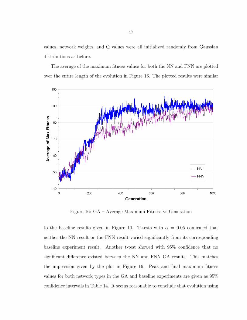
47
values, network weights, and Q values were all initialized randomly from Gaussian
distributions as before.
The average of the maximum fitness values for both the NN and FNN are plotted
over the entire length of the evolution in Figure 16. The plotted results were similar
Figure 16: GA – Average Maximum Fitness vs Generation
to the baseline results given in Figure 10. T-tests with α = 0.05 confirmed that
neither the NN result or the FNN result varied significantly from its corresponding
baseline experiment result. Another t-test showed with 95% confidence that no
significant difference existed between the NN and FNN GA results. This matches
the impression given by the plot in Figure 16. Peak and final maximum fitness
values for both network types in the GA and baseline experiments are given as 95%
confidence intervals in Table 14. It seems reasonable to conclude that evolution using
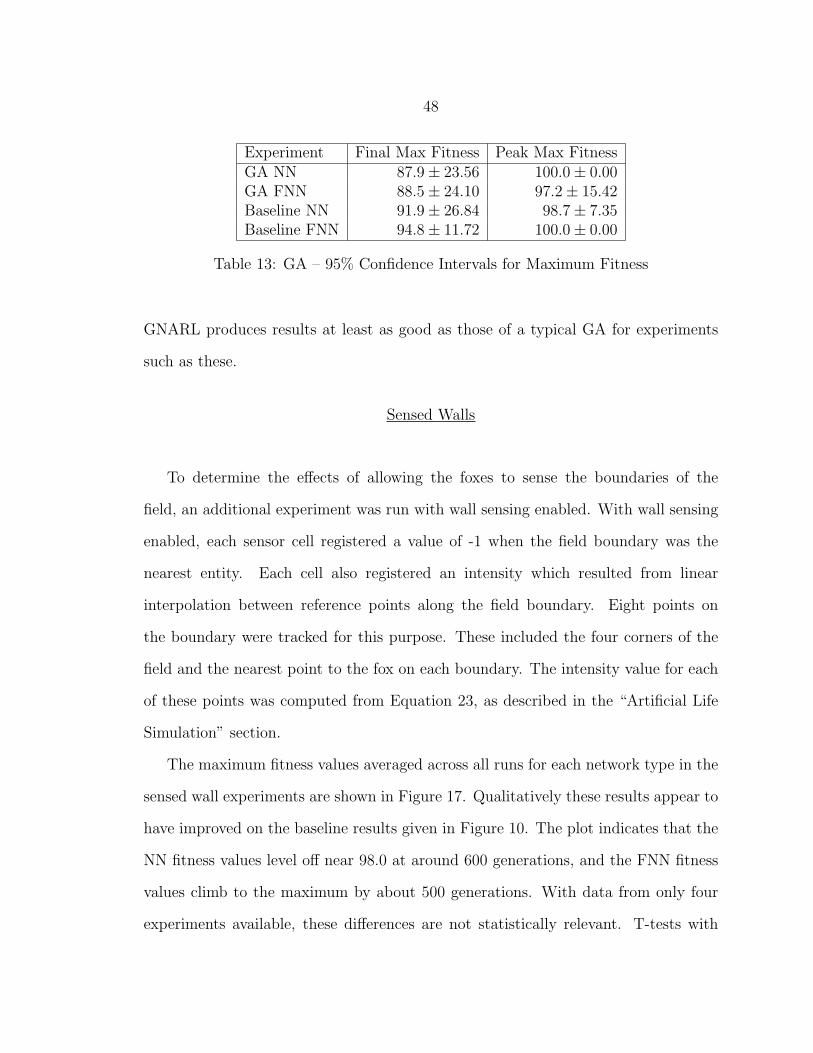
48
Experiment Final Max Fitness Peak Max FitnessGA NN 87.9± 23.56 100.0± 0.00GA FNN 88.5± 24.10 97.2± 15.42Baseline NN 91.9± 26.84 98.7± 7.35Baseline FNN 94.8± 11.72 100.0± 0.00
Table 13: GA – 95% Confidence Intervals for Maximum Fitness
GNARL produces results at least as good as those of a typical GA for experiments
such as these.
Sensed Walls
To determine the effects of allowing the foxes to sense the boundaries of the
field, an additional experiment was run with wall sensing enabled. With wall sensing
enabled, each sensor cell registered a value of -1 when the field boundary was the
nearest entity. Each cell also registered an intensity which resulted from linear
interpolation between reference points along the field boundary. Eight points on
the boundary were tracked for this purpose. These included the four corners of the
field and the nearest point to the fox on each boundary. The intensity value for each
of these points was computed from Equation 23, as described in the “Artificial Life
Simulation” section.
The maximum fitness values averaged across all runs for each network type in the
sensed wall experiments are shown in Figure 17. Qualitatively these results appear to
have improved on the baseline results given in Figure 10. The plot indicates that the
NN fitness values level off near 98.0 at around 600 generations, and the FNN fitness
values climb to the maximum by about 500 generations. With data from only four
experiments available, these differences are not statistically relevant. T-tests with
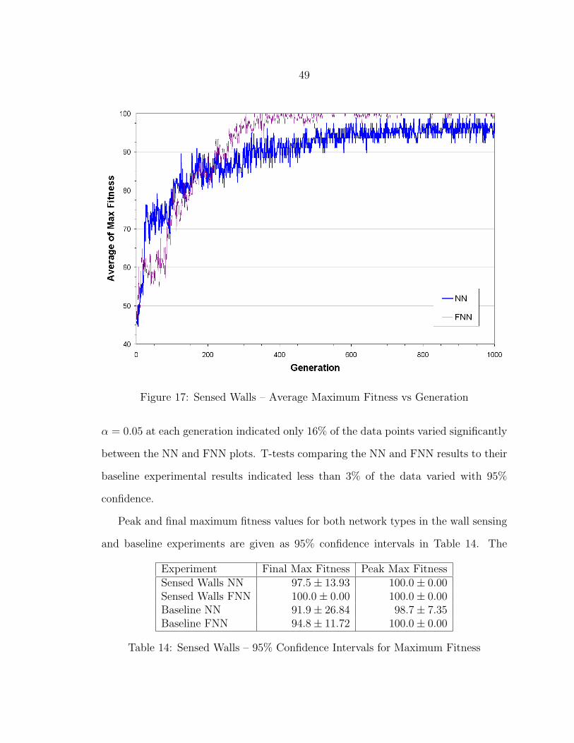
49
Figure 17: Sensed Walls – Average Maximum Fitness vs Generation
α = 0.05 at each generation indicated only 16% of the data points varied significantly
between the NN and FNN plots. T-tests comparing the NN and FNN results to their
baseline experimental results indicated less than 3% of the data varied with 95%
confidence.
Peak and final maximum fitness values for both network types in the wall sensing
and baseline experiments are given as 95% confidence intervals in Table 14. The
Experiment Final Max Fitness Peak Max FitnessSensed Walls NN 97.5± 13.93 100.0± 0.00Sensed Walls FNN 100.0± 0.00 100.0± 0.00Baseline NN 91.9± 26.84 98.7± 7.35Baseline FNN 94.8± 11.72 100.0± 0.00
Table 14: Sensed Walls – 95% Confidence Intervals for Maximum Fitness
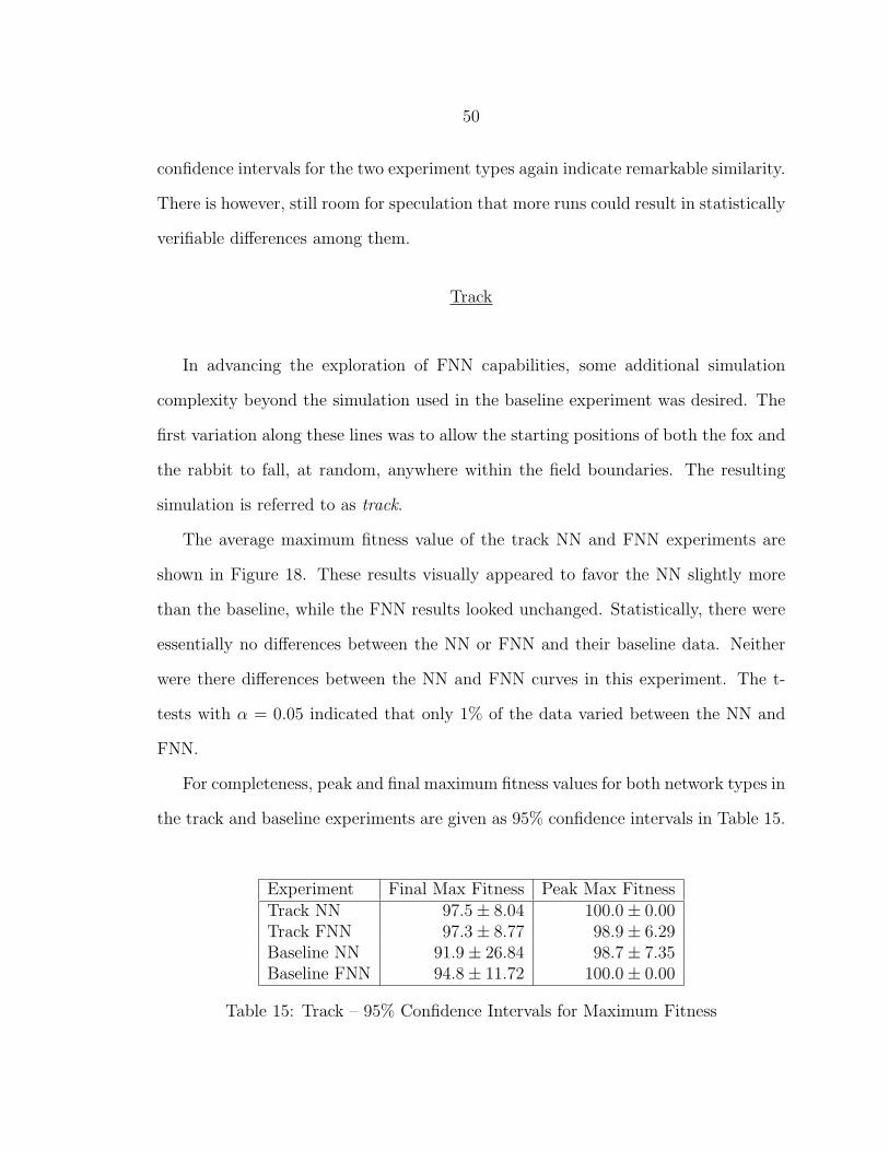
50
confidence intervals for the two experiment types again indicate remarkable similarity.
There is however, still room for speculation that more runs could result in statistically
verifiable differences among them.
Track
In advancing the exploration of FNN capabilities, some additional simulation
complexity beyond the simulation used in the baseline experiment was desired. The
first variation along these lines was to allow the starting positions of both the fox and
the rabbit to fall, at random, anywhere within the field boundaries. The resulting
simulation is referred to as track.
The average maximum fitness value of the track NN and FNN experiments are
shown in Figure 18. These results visually appeared to favor the NN slightly more
than the baseline, while the FNN results looked unchanged. Statistically, there were
essentially no differences between the NN or FNN and their baseline data. Neither
were there differences between the NN and FNN curves in this experiment. The t-
tests with α = 0.05 indicated that only 1% of the data varied between the NN and
FNN.
For completeness, peak and final maximum fitness values for both network types in
the track and baseline experiments are given as 95% confidence intervals in Table 15.
Experiment Final Max Fitness Peak Max FitnessTrack NN 97.5± 8.04 100.0± 0.00Track FNN 97.3± 8.77 98.9± 6.29Baseline NN 91.9± 26.84 98.7± 7.35Baseline FNN 94.8± 11.72 100.0± 0.00
Table 15: Track – 95% Confidence Intervals for Maximum Fitness
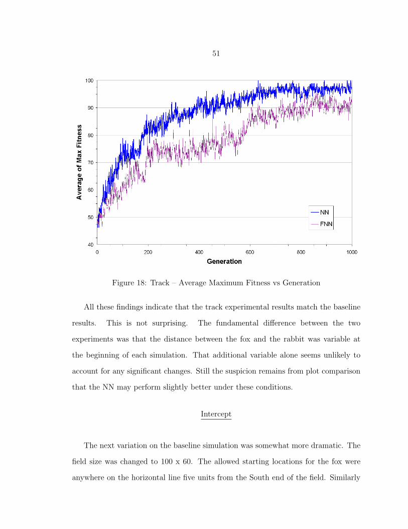
51
Figure 18: Track – Average Maximum Fitness vs Generation
All these findings indicate that the track experimental results match the baseline
results. This is not surprising. The fundamental difference between the two
experiments was that the distance between the fox and the rabbit was variable at
the beginning of each simulation. That additional variable alone seems unlikely to
account for any significant changes. Still the suspicion remains from plot comparison
that the NN may perform slightly better under these conditions.
Intercept
The next variation on the baseline simulation was somewhat more dramatic. The
field size was changed to 100 x 60. The allowed starting locations for the fox were
anywhere on the horizontal line five units from the South end of the field. Similarly
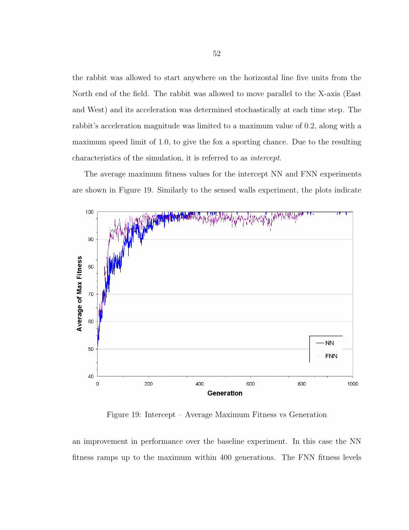
52
the rabbit was allowed to start anywhere on the horizontal line five units from the
North end of the field. The rabbit was allowed to move parallel to the X-axis (East
and West) and its acceleration was determined stochastically at each time step. The
rabbit’s acceleration magnitude was limited to a maximum value of 0.2, along with a
maximum speed limit of 1.0, to give the fox a sporting chance. Due to the resulting
characteristics of the simulation, it is referred to as intercept.
The average maximum fitness values for the intercept NN and FNN experiments
are shown in Figure 19. Similarly to the sensed walls experiment, the plots indicate
Figure 19: Intercept – Average Maximum Fitness vs Generation
an improvement in performance over the baseline experiment. In this case the NN
fitness ramps up to the maximum within 400 generations. The FNN fitness levels
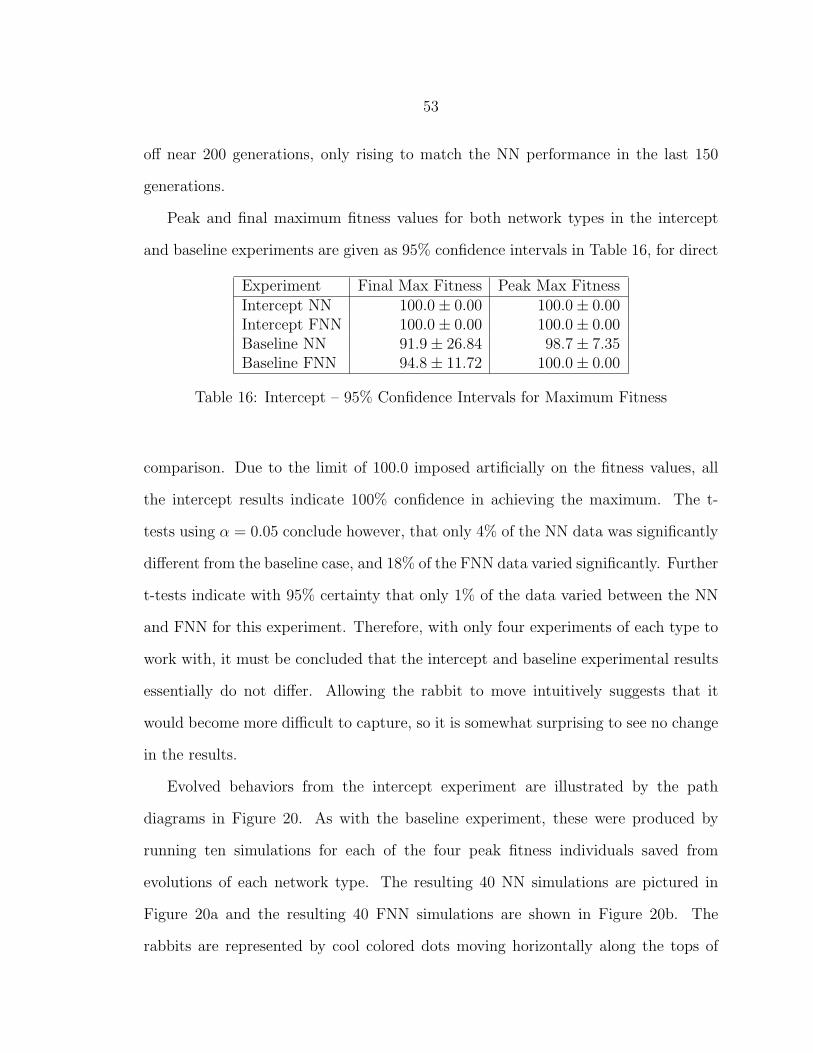
53
off near 200 generations, only rising to match the NN performance in the last 150
generations.
Peak and final maximum fitness values for both network types in the intercept
and baseline experiments are given as 95% confidence intervals in Table 16, for direct
Experiment Final Max Fitness Peak Max FitnessIntercept NN 100.0± 0.00 100.0± 0.00Intercept FNN 100.0± 0.00 100.0± 0.00Baseline NN 91.9± 26.84 98.7± 7.35Baseline FNN 94.8± 11.72 100.0± 0.00
Table 16: Intercept – 95% Confidence Intervals for Maximum Fitness
comparison. Due to the limit of 100.0 imposed artificially on the fitness values, all
the intercept results indicate 100% confidence in achieving the maximum. The t-
tests using α = 0.05 conclude however, that only 4% of the NN data was significantly
different from the baseline case, and 18% of the FNN data varied significantly. Further
t-tests indicate with 95% certainty that only 1% of the data varied between the NN
and FNN for this experiment. Therefore, with only four experiments of each type to
work with, it must be concluded that the intercept and baseline experimental results
essentially do not differ. Allowing the rabbit to move intuitively suggests that it
would become more difficult to capture, so it is somewhat surprising to see no change
in the results.
Evolved behaviors from the intercept experiment are illustrated by the path
diagrams in Figure 20. As with the baseline experiment, these were produced by
running ten simulations for each of the four peak fitness individuals saved from
evolutions of each network type. The resulting 40 NN simulations are pictured in
Figure 20a and the resulting 40 FNN simulations are shown in Figure 20b. The
rabbits are represented by cool colored dots moving horizontally along the tops of
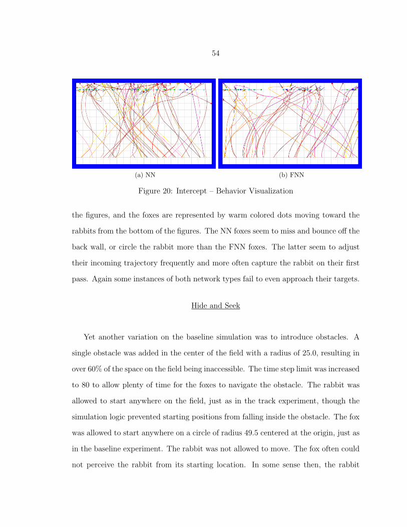
54
(a) NN (b) FNN
Figure 20: Intercept – Behavior Visualization
the figures, and the foxes are represented by warm colored dots moving toward the
rabbits from the bottom of the figures. The NN foxes seem to miss and bounce off the
back wall, or circle the rabbit more than the FNN foxes. The latter seem to adjust
their incoming trajectory frequently and more often capture the rabbit on their first
pass. Again some instances of both network types fail to even approach their targets.
Hide and Seek
Yet another variation on the baseline simulation was to introduce obstacles. A
single obstacle was added in the center of the field with a radius of 25.0, resulting in
over 60% of the space on the field being inaccessible. The time step limit was increased
to 80 to allow plenty of time for the foxes to navigate the obstacle. The rabbit was
allowed to start anywhere on the field, just as in the track experiment, though the
simulation logic prevented starting positions from falling inside the obstacle. The fox
was allowed to start anywhere on a circle of radius 49.5 centered at the origin, just as
in the baseline experiment. The rabbit was not allowed to move. The fox often could
not perceive the rabbit from its starting location. In some sense then, the rabbit

55
was hiding, and the fox’s task was to seek it out and capture it. This simulation is
referred to as hide and seek.
Faced with these odds, it may come as no surprise that the hide and seek evolution
was unsuccessful. The average maximum fitness values for both the NN and FNN
remained relatively constant throughout the evolution as illustrated in Figure 21.
Figure 21: Hide and Seek – Average Maximum Fitness vs Generation
Although the flat fitness curve indicates a failure to evolve, the path diagrams
shown in Figure 22 provide some insight into behaviors that did develop. These were
generated using the same method as in previous experiments. Ten simulations per
peak fitness individual were run resulting in 40 for each network type. The NNs in
Figure 22a exhibited an “orbiting” behavior which served to capture the rabbit by
way of covering lots of area quickly. The FNNs in Figure 22b had adopted more of a
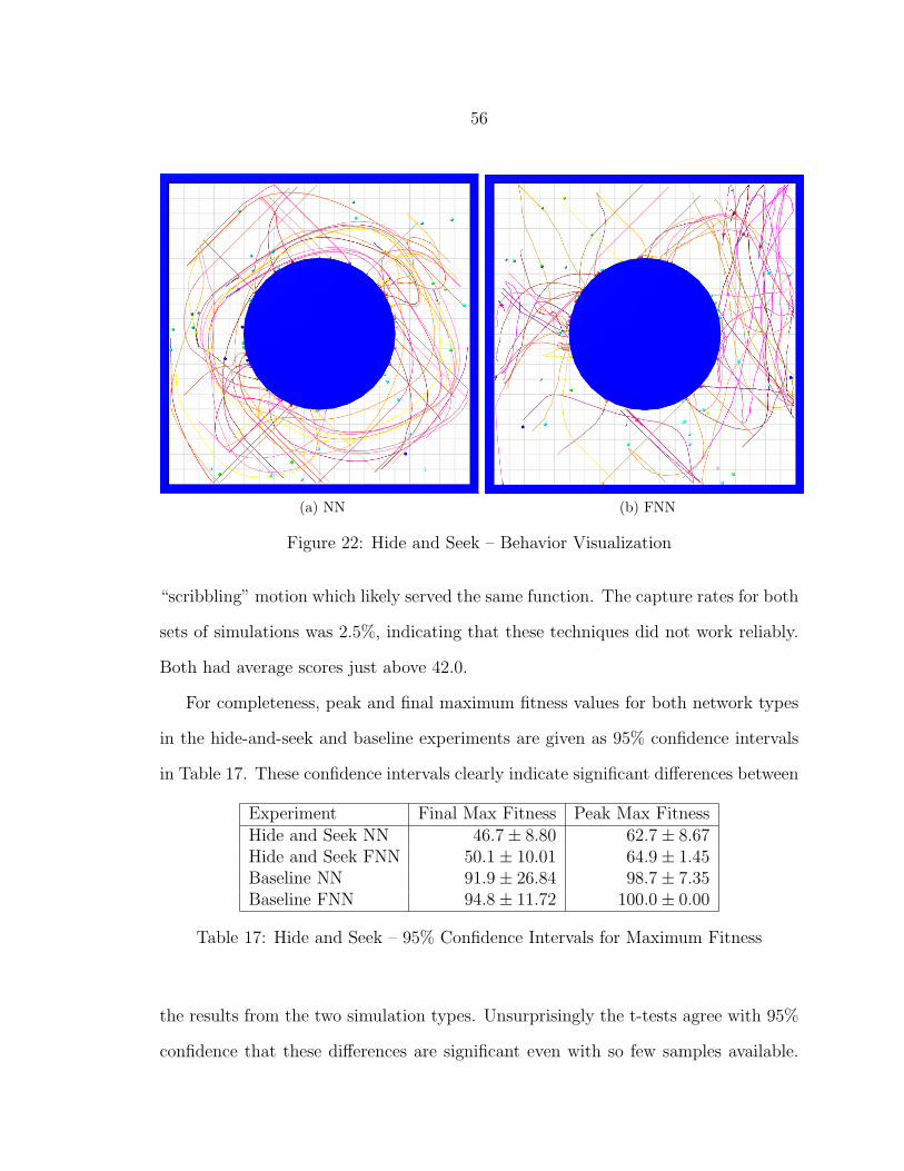
56
(a) NN (b) FNN
Figure 22: Hide and Seek – Behavior Visualization
“scribbling” motion which likely served the same function. The capture rates for both
sets of simulations was 2.5%, indicating that these techniques did not work reliably.
Both had average scores just above 42.0.
For completeness, peak and final maximum fitness values for both network types
in the hide-and-seek and baseline experiments are given as 95% confidence intervals
in Table 17. These confidence intervals clearly indicate significant differences between
Experiment Final Max Fitness Peak Max FitnessHide and Seek NN 46.7± 8.80 62.7± 8.67Hide and Seek FNN 50.1± 10.01 64.9± 1.45Baseline NN 91.9± 26.84 98.7± 7.35Baseline FNN 94.8± 11.72 100.0± 0.00
Table 17: Hide and Seek – 95% Confidence Intervals for Maximum Fitness
the results from the two simulation types. Unsurprisingly the t-tests agree with 95%
confidence that these differences are significant even with so few samples available.
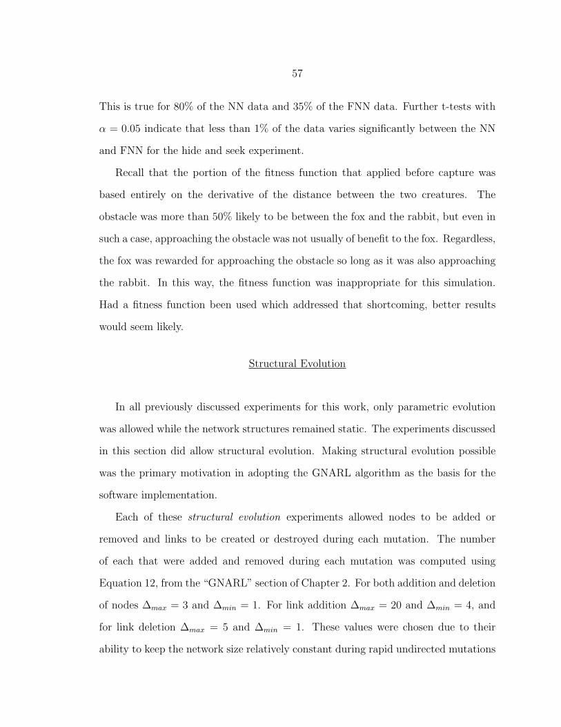
57
This is true for 80% of the NN data and 35% of the FNN data. Further t-tests with
α = 0.05 indicate that less than 1% of the data varies significantly between the NN
and FNN for the hide and seek experiment.
Recall that the portion of the fitness function that applied before capture was
based entirely on the derivative of the distance between the two creatures. The
obstacle was more than 50% likely to be between the fox and the rabbit, but even in
such a case, approaching the obstacle was not usually of benefit to the fox. Regardless,
the fox was rewarded for approaching the obstacle so long as it was also approaching
the rabbit. In this way, the fitness function was inappropriate for this simulation.
Had a fitness function been used which addressed that shortcoming, better results
would seem likely.
Structural Evolution
In all previously discussed experiments for this work, only parametric evolution
was allowed while the network structures remained static. The experiments discussed
in this section did allow structural evolution. Making structural evolution possible
was the primary motivation in adopting the GNARL algorithm as the basis for the
software implementation.
Each of these structural evolution experiments allowed nodes to be added or
removed and links to be created or destroyed during each mutation. The number
of each that were added and removed during each mutation was computed using
Equation 12, from the “GNARL” section of Chapter 2. For both addition and deletion
of nodes ∆max = 3 and ∆min = 1. For link addition ∆max = 20 and ∆min = 4, and
for link deletion ∆max = 5 and ∆min = 1. These values were chosen due to their
ability to keep the network size relatively constant during rapid undirected mutations
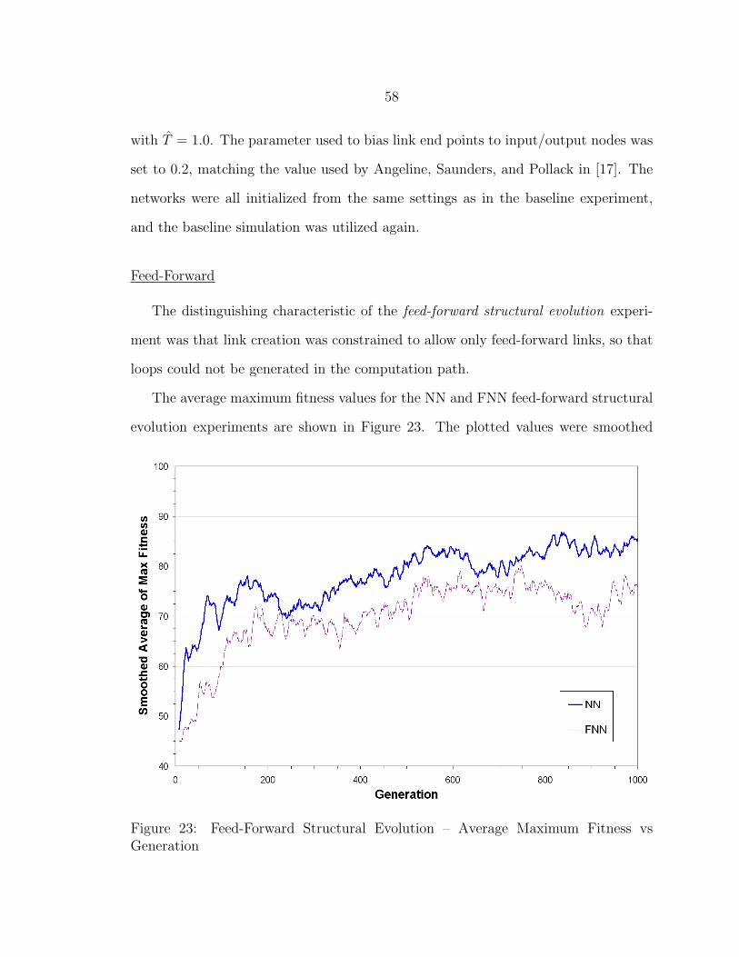
58
with T = 1.0. The parameter used to bias link end points to input/output nodes was
set to 0.2, matching the value used by Angeline, Saunders, and Pollack in [17]. The
networks were all initialized from the same settings as in the baseline experiment,
and the baseline simulation was utilized again.
Feed-Forward
The distinguishing characteristic of the feed-forward structural evolution experi-
ment was that link creation was constrained to allow only feed-forward links, so that
loops could not be generated in the computation path.
The average maximum fitness values for the NN and FNN feed-forward structural
evolution experiments are shown in Figure 23. The plotted values were smoothed
Figure 23: Feed-Forward Structural Evolution – Average Maximum Fitness vsGeneration

59
using a moving average with a window size of nine. Visually the FNN fitness appeared
to trail the NN fitness by approximately ten points throughout the evolution and both
curves showed less fit final results after 1000 generations than the baseline experiment.
Peak and final maximum fitness values for both network types in the feed-forward
structural and baseline experiments are given as 95% confidence intervals in Table 18.
The confidence intervals seem to indicate an improvement over the baseline results
Experiment Final Max Fitness Peak Max FitnessFeed-Forward Structural NN 90.3± 15.55 100.0± 0.00Feed-Forward Structural FNN 86.9± 28.00 95.7± 15.41Baseline NN 91.9± 26.84 98.7± 7.35Baseline FNN 94.8± 11.72 100.0± 0.00
Table 18: Feed-Forward Structural – 95% Confidence Intervals for Maximum Fitness
for the NN, with a decrease in fitness results for the FNN. However, the t-tests with
α = 0.05 show essentially no significant difference between the feed-forward structural
data and the baseline data. They also show absolutely no verifiable difference between
the NN and FNN for this experiment.
The average number of nodes and links in the four peak fitness networks saved
from both the NN and FNN evolutions were computed. For both network types, the
average number of nodes was 37.25. The average number of links were 62.75 and
54.25 for the NN and FNN respectively. By comparison, the feed-forward topology
used in the baseline experiment included 37 total nodes and 272 links. The structural
evolution maintained roughly the same number of nodes (though not necessarily in the
computation path). The average number of links in peak fitness individuals however,
was reduced to roughly 20% of the original number.
In the feed-forward structural evolution experiments, few possibilities for addi-
tional links existed for the initial networks. Most of the allowed connections already
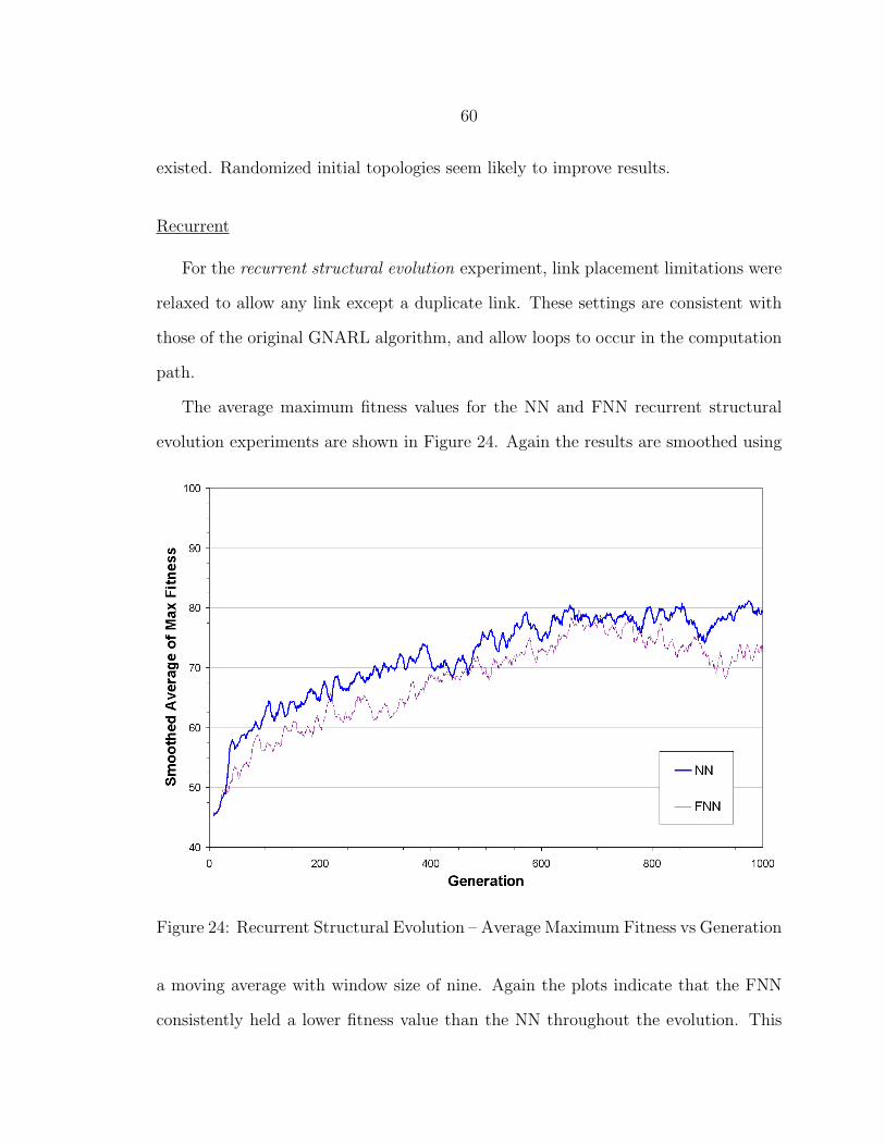
60
existed. Randomized initial topologies seem likely to improve results.
Recurrent
For the recurrent structural evolution experiment, link placement limitations were
relaxed to allow any link except a duplicate link. These settings are consistent with
those of the original GNARL algorithm, and allow loops to occur in the computation
path.
The average maximum fitness values for the NN and FNN recurrent structural
evolution experiments are shown in Figure 24. Again the results are smoothed using
Figure 24: Recurrent Structural Evolution – Average Maximum Fitness vs Generation
a moving average with window size of nine. Again the plots indicate that the FNN
consistently held a lower fitness value than the NN throughout the evolution. This
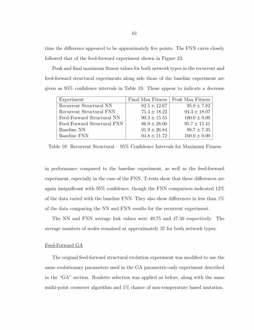
61
time the difference appeared to be approximately five points. The FNN curve closely
followed that of the feed-forward experiment shown in Figure 23.
Peak and final maximum fitness values for both network types in the recurrent and
feed-forward structural experiments along side those of the baseline experiment are
given as 95% confidence intervals in Table 19. These appear to indicate a decrease
Experiment Final Max Fitness Peak Max FitnessRecurrent Structural NN 82.5± 12.67 95.8± 7.82Recurrent Structural FNN 75.4± 18.22 94.3± 18.07Feed-Forward Structural NN 90.3± 15.55 100.0± 0.00Feed-Forward Structural FNN 86.9± 28.00 95.7± 15.41Baseline NN 91.9± 26.84 98.7± 7.35Baseline FNN 94.8± 11.72 100.0± 0.00
Table 19: Recurrent Structural – 95% Confidence Intervals for Maximum Fitness
in performance compared to the baseline experiment, as well as the feed-forward
experiment, especially in the case of the FNN. T-tests show that these differences are
again insignificant with 95% confidence, though the FNN comparison indicated 12%
of the data varied with the baseline FNN. They also show differences in less than 1%
of the data comparing the NN and FNN results for the recurrent experiment.
The NN and FNN average link values were 49.75 and 47.50 respectively. The
average numbers of nodes remained at approximately 37 for both network types.
Feed-Forward GA
The original feed-forward structural evolution experiment was modified to use the
same evolutionary parameters used in the GA parametric-only experiment described
in the “GA” section. Roulette selection was applied as before, along with the same
multi-point crossover algorithm and 1% chance of non-temperature based mutation.
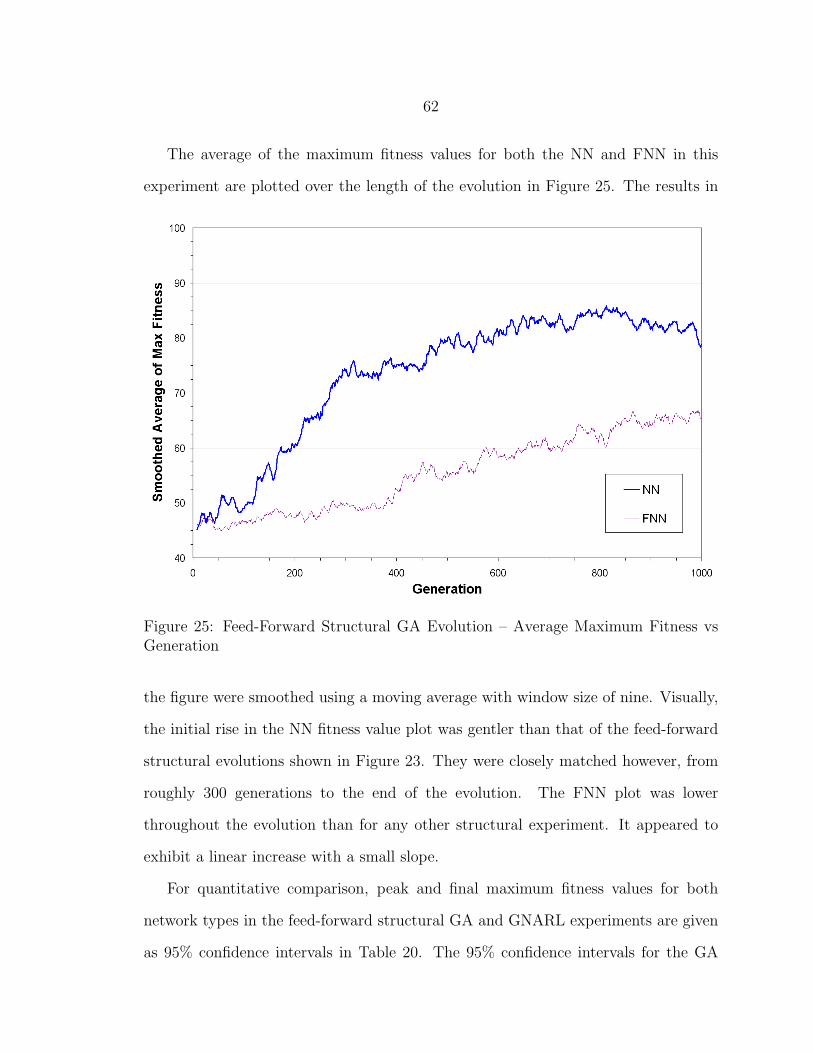
62
The average of the maximum fitness values for both the NN and FNN in this
experiment are plotted over the length of the evolution in Figure 25. The results in
Figure 25: Feed-Forward Structural GA Evolution – Average Maximum Fitness vsGeneration
the figure were smoothed using a moving average with window size of nine. Visually,
the initial rise in the NN fitness value plot was gentler than that of the feed-forward
structural evolutions shown in Figure 23. They were closely matched however, from
roughly 300 generations to the end of the evolution. The FNN plot was lower
throughout the evolution than for any other structural experiment. It appeared to
exhibit a linear increase with a small slope.
For quantitative comparison, peak and final maximum fitness values for both
network types in the feed-forward structural GA and GNARL experiments are given
as 95% confidence intervals in Table 20. The 95% confidence intervals for the GA
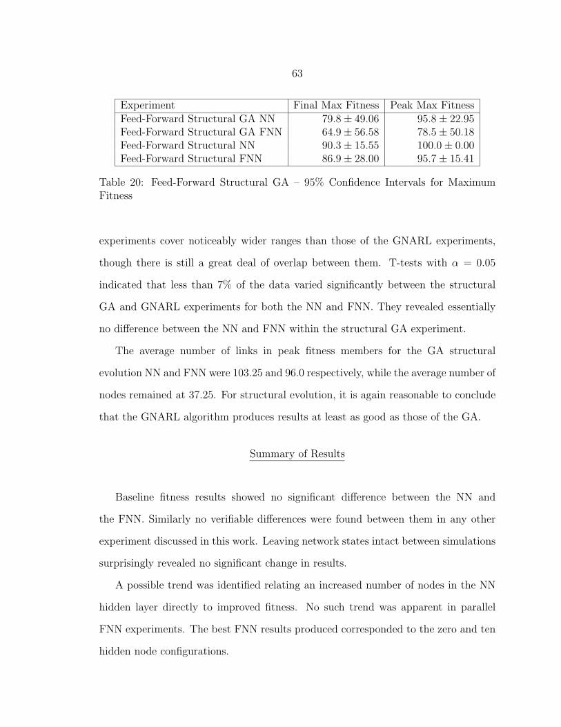
63
Experiment Final Max Fitness Peak Max FitnessFeed-Forward Structural GA NN 79.8± 49.06 95.8± 22.95Feed-Forward Structural GA FNN 64.9± 56.58 78.5± 50.18Feed-Forward Structural NN 90.3± 15.55 100.0± 0.00Feed-Forward Structural FNN 86.9± 28.00 95.7± 15.41
Table 20: Feed-Forward Structural GA – 95% Confidence Intervals for MaximumFitness
experiments cover noticeably wider ranges than those of the GNARL experiments,
though there is still a great deal of overlap between them. T-tests with α = 0.05
indicated that less than 7% of the data varied significantly between the structural
GA and GNARL experiments for both the NN and FNN. They revealed essentially
no difference between the NN and FNN within the structural GA experiment.
The average number of links in peak fitness members for the GA structural
evolution NN and FNN were 103.25 and 96.0 respectively, while the average number of
nodes remained at 37.25. For structural evolution, it is again reasonable to conclude
that the GNARL algorithm produces results at least as good as those of the GA.
Summary of Results
Baseline fitness results showed no significant difference between the NN and
the FNN. Similarly no verifiable differences were found between them in any other
experiment discussed in this work. Leaving network states intact between simulations
surprisingly revealed no significant change in results.
A possible trend was identified relating an increased number of nodes in the NN
hidden layer directly to improved fitness. No such trend was apparent in parallel
FNN experiments. The best FNN results produced corresponded to the zero and ten
hidden node configurations.
64
Tests with fixed Q values indicated that fitness results are negatively impacted
when using FNNs composed entirely of integrating units or 1st order derivative units.
The best results were produced using Q = 0.25. Evolving networks with variable Q
values also returned high fitness results.
GNARL evolution produced results at least as good as the GA results for both
fixed topology and evolved topology experiments with 95% confidence. No differences
between the NN and FNN fitness data were established which related to the choice
of evolutionary algorithm.
Behaviorally, the NN and FNN tended to produce subtly different solutions to
each problem, but statistically significant differences between these behaviors were
not identified.
T-tests revealed with 95% confidence that no significant difference existed between
the results using the baseline simulation and those of any other simulation discussed
in this work, except for hide and seek. Both network types showed similar difficulty
in fitness evolution for the hide and seek experiment. Similarly, t-tests for the three
types of structural evolution tested also showed with 95% confidence no significant
differences in fitness results.
65
CHAPTER 5
FUTURE WORK
More Experimental Data
All the experimental data discussed in Chapter 4 is statistically limited in its
usefulness due to the small number of evolutions (4) run for each experiment. The
processing time required to run these experiments was prohibitive, which is why their
number was so limited. Running more, and longer experiments would improve upon
the results from this work.
More experiments and analysis regarding the differences in performance for
varying numbers of nodes in the hidden layer are desired. These would qualify
the existence of the identified trend in the NN experiments, and perhaps discover
a relationship between the number of nodes and the fitness results for the FNN.
Experiments could also be run on different topologies to detect further interesting
relationships.
Results for the fixed Q value results indicated that Q values in the approximate
range [0.0, 0.5] may correlate with improved fitness results. Informal observations
also indicated that evolved Q values tend to fall within that range. Not enough
statistical data was available to say whether these observations were meaningful.
More experimental data and the collection of network Q value composition statistics
in FNN experiments with variable Q values would correct the problem.
Verifying consistent differences in behavior between the NN and FNN, or the lack
thereof, would improve on one of the more interesting facets of this work. Behavioral
differences were observed, but whether or not they can be attributed to the difference
66
in network type remains to be shown.
Though no statistically relevant differences were found between the network types
on any discussed simulation, visual interpretation of the plots still suggests that such
differences may be verified with more available data. This seems particularly likely
for the sensed walls, track and structural GA experiments. As discussed, additional
data also seems likely to reveal quantifiable differences among hidden node size and
fixed q value experiments.
Structural Evolution
The GNARL algorithm was adopted as the basis for software implementation
in this work and a generalized multi-point crossover algorithm capable of handling
varying parent network topologies was developed. These and related efforts
were targeted at enabling automated topology design through evolution while
simultaneously adjusting network parameters for best fitness. Initial exploration of
structural evolution showed promising results, but due to time constraints evolution
parameters for the formal experiments discussed in this work were only minimally
tuned. Continuation of the work on structural evolution is still expected to produce
interesting results.
Backpropagation
In Chapter 2, the possibility of using backpropagation as a means of training FNNs
was mentioned. This still remains an interesting possibility. If successful, it would
allow more direct comparison of FNN learning characteristics with the many existing
systems which use backpropagation as a training mechanism. The concept remains

67
sound and adaptation of backpropagation to FNNs may be as simple as adding the
Q value of each node to the list of parameters that is adjusted using the propagated
error. The Q value of a node changes the relative effect of all the outgoing link weights
at once however, and may therefore require some special handling.
Fractional calculus may also be applied directly to the backpropagation algorithm
used in training un-augmented neural networks. Such an attempt was made in [29].
In that system, the weight update rule was augmented with proportional integral
and derivative (PID) control parameters acting on the inverse error gradient. The
fractional differintegral was then applied to both the integer and derivative PID
control terms resulting in PIλDµ control parameters. More useful behavior might
result from applying a differintegral operation to the gradient calculation, or to a
dynamic learning rate η. Should such a system be tuned to achieve a learning
performance gain, it would be equally well adapted to training FNNs as the basic
backpropagation algorithm.
Simulation Complexity
The vision held throughout this work, though perhaps naive, was to evolve
foxes with much richer behavioral characteristics. The original simulation involved
complicated energy use characteristics which would require the foxes to manage their
energy carefully so they would still have enough available when necessary for a short
but extreme speed burst in making a capture. The imagined behaviors that might
develop from these rules were many and varied. The foxes were expected to learn
enough to catch an evasive rabbit. Once that level of complexity was reached, the
rabbits could be evolved to improve their escape tactics. The foxes could then be

68
evolved to outperform the rabbits again, and so on. The system was designed to
allow simultaneous co-evolution to occur with this objective in mind.
A simpler sensor and movement model was proposed but not implemented. In
this model, the fox would face in a specific direction and would be allowed to rotate
or move forward or backward. Its sensor array would be pointed in the direction it
was facing so that it would have to turn to “see” more of its surroundings. Because
it would cover less area, the array could be composed of fewer sensors while still
providing the same quality perception of the environment. Much less redundant
learning would be required with sensors tightly coupled to movement.
The mechanism of evaluating each individual using a single value at the end of
several lengthy simulations creates a credit assignment problem which is difficult
to alleviate by adjusting the fitness function. A more direct approach would be to
implement online learning during each simulation. If weights and Q values were
adjusted at small intervals throughout the simulation the creatures would receive
more direct feed-back for their actions and more complex behaviors might become
accessible.
The fox/rabbit simulation implementation did not appear to exhibit the character-
istics necessary to make power-law modeling applicable. A simulation which directly
simulated power-law dynamics might produce better results.
69
CHAPTER 6
CONCLUSIONS
Fitness data for the NN and FNN showed with 95% confidence that no significant
difference existed between them for any simulation discussed in Chapter 4. The most
obvious conclusion that can be drawn from this is that more experimental data is
desired.
It was shown with 95% confidence that failing to reset FNN states between
simulations in the baseline experiment did not impact the fitness results. This result
was unexpected and may indicate a robustness to inconsistency in the FNN.
The hidden layer size experiment showed a possible trend relating improved fitness
results directly to an increased number of nodes in the NN’s hidden layer. No such
trend was apparent in the FNN hidden layer size experiment. Increasing the number of
nodes in the FNN’s hidden layer more often resulted in lower fitness values. Findings
showed that among the hidden node sizes tested, the zero and ten node configurations
produced the highest fitness results with 95% confidence.
Tests with fixed Q values indicated that fitness results are negatively impacted
when using FNNs composed entirely of integrating units or 1st order derivative
units. The best results among the fixed Q value experiments were produced using
Q = 0.25 on the baseline simulation. The available data indicated that a correlation
may exist between Q values in the approximate range [0.0, 0.5] and higher fitness
values. The necessary data to test this correlation with statistical relevance was not
available. Evolving networks with variable Q values was also found to produce better
results than many of the fixed Q value experiments. If an optimal configuration
of homogeneous Q values existed, the evolution of variable Q values might be
70
a reasonable way to discover it. Further, if the optimal Q value were problem
dependant, its automatic discovery would seem valuable.
GNARL based evolution produced results at least as good as the GA results for
both fixed topology and evolved topology experiments with 95% confidence. This
shows the choice of evolution to be an insignificant factor in the results.
Differences in fitness results among the five simulations tested in this work
appeared plausible based on visual analysis of plotted data. T-tests revealed with 95%
confidence that very little of the data varied significantly. The obvious exception was
the hide and seek simulation, which clearly produced different fitness results than the
baseline simulation. With more experimental data, some of these plausible differences
are expected to become verifiable.
The introduction of an obstacle to the simulation environment significantly
decreased fitness results in the hide and seek experiment. Adaptation of the fitness
evaluation function to account for the obstacle is expected to improve results. For the
evaluation to be effective, the fox must not be rewarded for approaching the rabbit
unless it can sense the rabbit.
Three types of structural evolution were tested on the baseline simulation. As
for other experiments, t-tests showed with 95% confidence that the results did
not vary significantly from those of the baseline, or from each other. Based on
visual interpretation of the fitness plots, a verifiable difference between the NN
and FNN fitness results appeared plausible for all three experiments. This was
particularly true in the case of the feed-forward structural GA experiments. With
only four evolutions for each network type and experiment, these differences were not
statistically significant but are expected to become so with slightly more data.
Differences in behavior were observed between the NN and FNN for each
simulation. Whether the differences could be attributed to the change in network
71
type was not determined, nor were any behavioral differences identified as statistically
significant. This remains as a point of future research.
The FNN tested in this work has shown fitness results comparable to those
of the NN in one artificial life simulation. However, no significant advantages of
the intended benefits added by the fractional augmentation were observed. The
simulation tested may not have exhibited the necessary characteristics to benefit from
the hypothesized natural modeling capability or lossy long-term memory available in
the FNN. Differences in fitness results and behaviors between the NN and FNN were
implicated by the results but not statistically significant. Whether the augmentation
provides any significant advantages remains an open question.
Some exploration of fractional calculus as an augmentation to artificial neural
networks was achieved in this work. As with most exploration, many more questions
were raised than were answered and countless possibilities for continued exploration
remain.

72
REFERENCES
[1] W. Duch, “Towards comprehensive foundations of computational intelligence,”Challenges for Computational Intelligence, vol. 63, pp. 261–316, 2007.
[2] B. Hammer and T. Villmann, “Mathematical aspects of neural networks,” inEuropean Symposium of Artificial Neural Networks 2003, M. Verleysen, Ed.,2003, pp. 59–72.
[3] R. Setiono and W. K. Leow, “Pruned neural networks for regression,” inProceedings of the 6th Pacific Rim Conference on Artificial Intelligence, PRICAI2000, Lecture Notes in AI 1886, 2000, pp. 500–509.
[4] K.-C. Jim, C. L. Giles, and B. G. Horne, “An analysis of noise in recurrentneural networks: Convergence and generalization,” IEEE Transactions on NeuralNetworks, vol. 7, pp. 1424–1439, 1996.
[5] M. J. L. Orr, “Introduction to radial basis function networks,” Centre forCognitive Science, University of Edinburgh, Tech. Rep., 1996.
[6] T. Kohonen, “Automatic formation of topological maps of patterns in a self-organizing system,” in Proceedings of 2nd Scandinavian Conference on ImageAnalysis, Espoo, Finland, 1981, pp. 214–220.
[7] J. J. Hopfield, “Neural networks and physical systems with emergent collectivecomputational abilites,” Proceedings of National Academy of Science, USA,vol. 79, pp. 2554–2558, 1982.
[8] L. O. Chua, “Cellular neural networks: Theory,” IEEE Transactions On CircuitsAnd Systems, vol. 35, no. 10, pp. 1257–1272, 1988.
[9] J. Baxter, “The evolution of learning algorithms for artificial neural networks,”in Complex Systems, G. D. and B. T., Eds. IOS Press, 1992, pp. 313–326.
[10] T. D. Sanger, “Optimal unsupervised learning in a single-layer linear feedforwardneural network,” Neural Networks, vol. 2, pp. 459–473, 1989.
[11] G. W. Bohannan, “Application of fractional calculus to polarization dynamicsin solid dielectric materials,” Ph.D. dissertation, Montana State University,Bozeman, Montana, November 2000.
[12] Y. Chen, B. M. Vinagre, and I. Podlubny, “Fractional order disturbance observerfor robust vibration suppression,” Nonlinear Dynamics, vol. 38, no. 1–2, pp. 355–367, 2004.
73
[13] Y. Chen, “Ubiquitous fractional order controls?” in The Second IFACSymposium on Fractional Derivatives and Applications (IFAC FDA06), JUL2006.
[14] J. A. T. Machado, “Analysis and design of fractional-order digital control sys-tems,” in SAMS - Journal Systems Analysis-Modeling-Simulation. Edinburgh:OPA (Overseas Publishers Association), 1997, vol. 27, pp. 107–122.
[15] X. Yao, “Evolving artificial neural networks,” in Proceedings of the IEEE, vol. 87,no. 9, 1999, pp. 1423–1447.
[16] X. Yao and Y. Liu, “Towards designing artificial neural networks by evolution,”Applied Mathematics and Computation, vol. 91, pp. 83–90, 1998.
[17] P. J. Angeline, G. M. Saunders, and J. P. Pollack, “An evolutionary algorithmthat constructs recurrent neural networks,” IEEE Transactions on NeuralNetworks, vol. 5, no. 1, pp. 54–65, JAN 1994.
[18] B. Krose and P. Van Der Smagt, An Introduction to Neural Networks, 8th ed.The University of Amsterdam, 2006, pp. 15–31, 33–46.
[19] P. J. Werbos, The Roots of Backpropagation: From Ordered Derivatives to NeuralNetworks and Political Forecasting. Wiley, John & Sons, Inc., 1994.
[20] M. Boden, “A guide to recurrent neural networks and backpropagation,” in TheDallas project, SICS Technical Report T2002:03, SICS, 2002.
[21] T. M. Mitchell, Machine Learning. WCB/McGraw-Hill, 2007, pp. 81–124.
[22] S. Kirkpatrick, C. D. Gelatt, and M. P. Vecchi, “Optimization by simulatedannealing,” Science, vol. 220, no. 4598, pp. 671–680, MAY 1983.
[23] R. Storn and K. Price, “Differential evolution - a simple and efficient heuristicfor global optimization over continuous spaces,” Journal of Global Optimization,vol. 11, no. 4, pp. 341–359, 1997.
[24] K. A. D. Jong, “An analysis of the behavior of a class of genetic adaptivesystems,” Ph.D. dissertation, University of Michigan, Ann Arbor, 1975.
[25] M. Mitchell, S. Forrest, and J. H. Holland, “The royal road for genetic algorithms:Fitness landscapes and ga performance,” in Proceedings of the First EuropeanConference on Artificial Life. MIT Press, 1992, pp. 245–254.
[26] F. Carpenteri and F. Mainardi, Eds., Fractals and Fractional Calculus inContinuum Mechanics, ser. CISM Courses and Lectures. New York: Springer-Verlag New York, Inc., 1997, vol. 378, p. 224.
74
[27] K. B. Oldham and J. Spanier, The Fractional Calculus Theory and Applicationsof Differentiation and Integration to Arbitrary Order, ser. Mathematics in Scienceand Engineering, R. Bellman, Ed. Academic Press, Inc., 1974, vol. 111.
[28] C. A. Monje, A. J. Calderon, B. M. Vinagre, Y. Chen, and V. Felıu,“On fractional piλ controllers: Some tuning rules for robustness to plantuncertainties,” Nonlinear Dynamics, vol. 38, no. 1–2, pp. 369–381, 2004.
[29] S. Gardner, R. Lamb, and J. Paxton, “An initial investigation on the useof fractional calculus with neural networks,” in Proceedings of the IASTEDInternational Conference COMPUTATIONAL INTELLIGENCE, NOV 2006,pp. 182–187.

75
APPENDICES

76
Appendix A
SOFTWARE
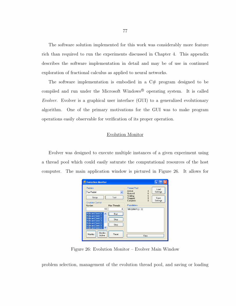
77
The software solution implemented for this work was considerably more feature
rich than required to run the experiments discussed in Chapter 4. This appendix
describes the software implementation in detail and may be of use in continued
exploration of fractional calculus as applied to neural networks.
The software implementation is embodied in a C# program designed to be
compiled and run under the Microsoft Windows R© operating system. It is called
Evolver. Evolver is a graphical user interface (GUI) to a generalized evolutionary
algorithm. One of the primary motivations for the GUI was to make program
operations easily observable for verification of its proper operation.
Evolution Monitor
Evolver was designed to execute multiple instances of a given experiment using
a thread pool which could easily saturate the computational resources of the host
computer. The main application window is pictured in Figure 26. It allows for
Figure 26: Evolution Monitor – Evolver Main Window
problem selection, management of the evolution thread pool, and saving or loading

78
of evolution settings. Interfaces to other parts of the program can also be spawned
from the main window.
The problem selector in the upper left allows the problem definition to be changed
at runtime. The original plan for this work was to study FNNs in multiple problem
domains, but the work required to get high quality results from one problem turned
out to be more than enough. Other problems toyed with during development include
spatial classification functions, sine wave generation, and predator/prey co-evolution.
Only the fox/rabbit problem definition is fully functional in the current version of
Evolver.
The “Evolution Control” section of the main window allows the user to specify
how many evolution instances to run, and how many threads to make available in the
thread pool. The list view displays all evolutions in the experiment. Any subset of
these may be selected for manipulation as a group. They may be started, stopped,
or stepped one generation at a time. Monitor windows may be spawned for progress
overviews and current status of each evolution. The “Reset” button clears all current
evolutions so that new ones can be started with the current settings. A red message
appears above this button to indicate when settings have been changed that require
a reset to take effect.
The thread pool information displayed in the upper right section of the window
provides a quick overview of what’s going on in the thread pool. This indicates the
current number of running or active threads. It also shows the number of evolutions
in the queue, the number which are waiting and ready to run as soon as a thread
becomes available, and the number which have been stopped by the user. The number
of completed evolutions is also provided.
The population view lists all the populations that exist in each of the running
evolutions. Any set of populations in the running evolutions may be viewed by
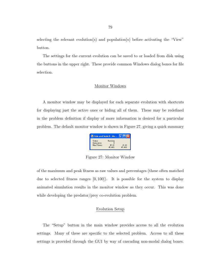
79
selecting the relevant evolution(s) and population(s) before activating the “View”
button.
The settings for the current evolution can be saved to or loaded from disk using
the buttons in the upper right. These provide common Windows dialog boxes for file
selection.
Monitor Windows
A monitor window may be displayed for each separate evolution with shortcuts
for displaying just the active ones or hiding all of them. These may be redefined
in the problem definition if display of more information is desired for a particular
problem. The default monitor window is shown in Figure 27, giving a quick summary
Figure 27: Monitor Window
of the maximum and peak fitness as raw values and percentages (these often matched
due to selected fitness ranges [0, 100]). It is possible for the system to display
animated simulation results in the monitor window as they occur. This was done
while developing the predator/prey co-evolution problem.
Evolution Setup
The “Setup” button in the main window provides access to all the evolution
settings. Many of these are specific to the selected problem. Access to all these
settings is provided through the GUI by way of cascading non-modal dialog boxes.

80
Figure 28 shows the general evolution settings dialog alongside the fox/rabbit problem
(a) General (b) Fox/Rabbit
Figure 28: Evolution Setting Setting Dialogs
specific evolution settings dialog. The general setup includes an evolution name
specification and stopping conditions. Logging options are also present to toggle
the generation of various output files. These range from the aggregated statistics
discussed in the “Statistic Collection” section at the end of Chapter 3, to peak fitness
individuals and whole populations.
A modifiable list of populations is also provided. Each population in the list will
be present in every evolution instance. The problem specific settings are accessed
by clicking the “Type Setup” button from the general settings dialog. Figure 28b
shows the result for the fox/rabbit problem used in this work. Here, the number of
simulation trials run for member evaluation can be specified. Some additional output
file selections for saving certain simulation replays to disk are also available. The
“Simulation” button provides access to all the fox/rabbit simulation settings which
will be discussed in the “Simulation Settings” subsection that follows.
When the user chooses to edit a population in the list, a dialog similar to the one

81
in Figure 29 is presented. This is the general population editing dialog, but member
Figure 29: Population Edit Dialog
types are controlled by the problem description. If the number of members added here
does not match the population size, each evolution instance fills the population with
randomly initialized members before the evolution begins. Some population type
specific settings may also exist. These are accessed by clicking the “Type Setup”
button.
The population type specific dialogs for the two available population types are
shown in Figure 30. The only setting provided in the GNARL population edit dialog
is the number of population members that survive to form each following generation
through mutation. This value is maintained as a percentage of the size when it is
changed in the main population edit dialog. The GA population edit dialog allows
a choice of selection algorithm, modification of some of the selection algorithms’
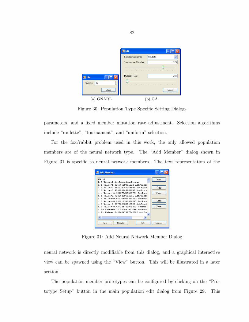
82
(a) GNARL (b) GA
Figure 30: Population Type Specific Setting Dialogs
parameters, and a fixed member mutation rate adjustment. Selection algorithms
include “roulette”, “tournament”, and “uniform” selection.
For the fox/rabbit problem used in this work, the only allowed population
members are of the neural network type. The “Add Member” dialog shown in
Figure 31 is specific to neural network members. The text representation of the
Figure 31: Add Neural Network Member Dialog
neural network is directly modifiable from this dialog, and a graphical interactive
view can be spawned using the “View” button. This will be illustrated in a later
section.
The population member prototypes can be configured by clicking on the “Pro-
totype Setup” button in the main population edit dialog from Figure 29. This
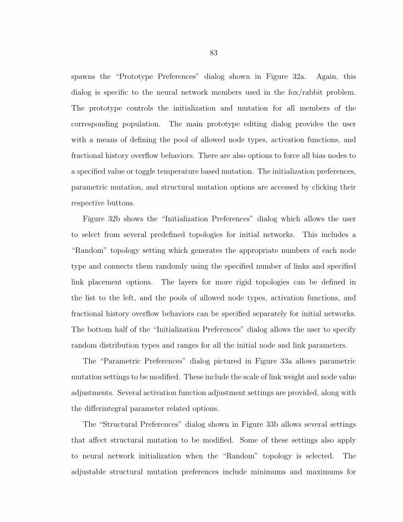
83
spawns the “Prototype Preferences” dialog shown in Figure 32a. Again, this
dialog is specific to the neural network members used in the fox/rabbit problem.
The prototype controls the initialization and mutation for all members of the
corresponding population. The main prototype editing dialog provides the user
with a means of defining the pool of allowed node types, activation functions, and
fractional history overflow behaviors. There are also options to force all bias nodes to
a specified value or toggle temperature based mutation. The initialization preferences,
parametric mutation, and structural mutation options are accessed by clicking their
respective buttons.
Figure 32b shows the “Initialization Preferences” dialog which allows the user
to select from several predefined topologies for initial networks. This includes a
“Random” topology setting which generates the appropriate numbers of each node
type and connects them randomly using the specified number of links and specified
link placement options. The layers for more rigid topologies can be defined in
the list to the left, and the pools of allowed node types, activation functions, and
fractional history overflow behaviors can be specified separately for initial networks.
The bottom half of the “Initialization Preferences” dialog allows the user to specify
random distribution types and ranges for all the initial node and link parameters.
The “Parametric Preferences” dialog pictured in Figure 33a allows parametric
mutation settings to be modified. These include the scale of link weight and node value
adjustments. Several activation function adjustment settings are provided, along with
the differintegral parameter related options.
The “Structural Preferences” dialog shown in Figure 33b allows several settings
that affect structural mutation to be modified. Some of these settings also apply
to neural network initialization when the “Random” topology is selected. The
adjustable structural mutation preferences include minimums and maximums for

84
(a) Main Prototype Settings
(b) Initialization Settings
Figure 32: Neural Network Prototype Preference Dialogs
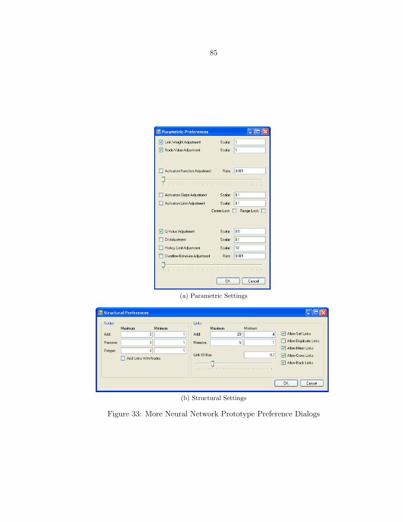
85
(a) Parametric Settings
(b) Structural Settings
Figure 33: More Neural Network Prototype Preference Dialogs

86
adding, removing and type changing of nodes. Link addition and removal count
ranges are also specified here, as well as the IO bias parameter. Allowed link types
are toggled on the right side.
Simulation Settings
The fox/rabbit simulation settings are accessible via the “Settings” button in the
fox/rabbit problem specific evolution settings dialog pictured in Figure 28b. The
resulting main simulation settings dialog is shown in Figure 34. It provides choices
Figure 34: Fox/Rabbit Simulation Settings Dialog
for the applied fitness function and options for simulation stopping conditions. The
type of both the fox and rabbit can be selected, although the problem is designed
to evolve the fox as a neural network, so other options should not be chosen in this
scope. Configuration dialogs for the field, and for both the fox and rabbit can be
spawned using their respective buttons.
The “Field” settings dialog pictured in Figure 35 allows the size of the simulation
field to be specified, along with a list of obstacles and their dimensions. An option
to toggle field boundaries, and one to toggle the creatures’ perception of them is also
provided here.
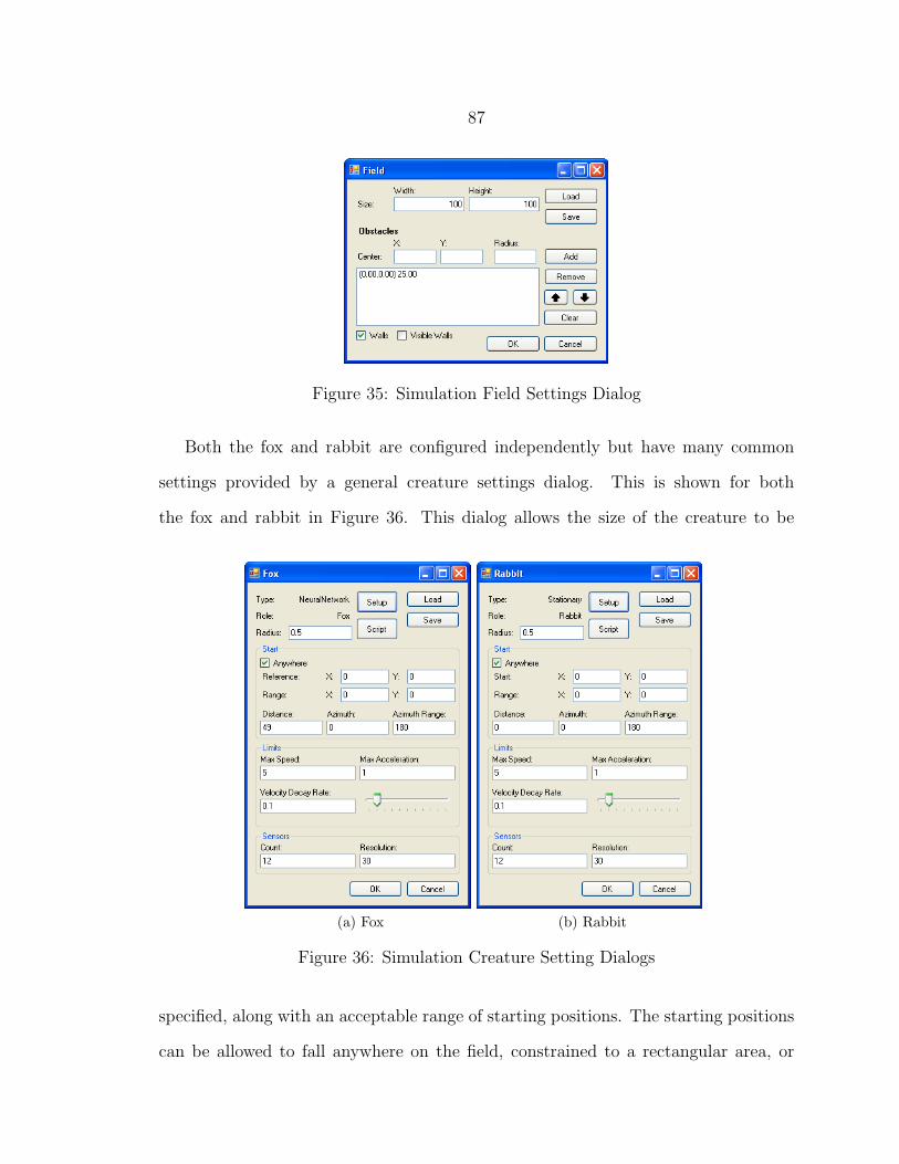
87
Figure 35: Simulation Field Settings Dialog
Both the fox and rabbit are configured independently but have many common
settings provided by a general creature settings dialog. This is shown for both
the fox and rabbit in Figure 36. This dialog allows the size of the creature to be
(a) Fox (b) Rabbit
Figure 36: Simulation Creature Setting Dialogs
specified, along with an acceptable range of starting positions. The starting positions
can be allowed to fall anywhere on the field, constrained to a rectangular area, or
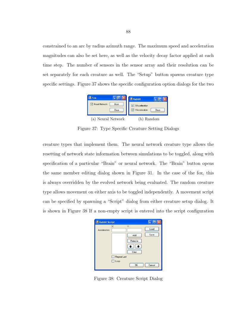
88
constrained to an arc by radius azimuth range. The maximum speed and acceleration
magnitudes can also be set here, as well as the velocity decay factor applied at each
time step. The number of sensors in the sensor array and their resolution can be
set separately for each creature as well. The “Setup” button spawns creature type
specific settings. Figure 37 shows the specific configuration option dialogs for the two
(a) Neural Network (b) Random
Figure 37: Type Specific Creature Setting Dialogs
creature types that implement them. The neural network creature type allows the
resetting of network state information between simulations to be toggled, along with
specification of a particular “Brain” or neural network. The “Brain” button opens
the same member editing dialog shown in Figure 31. In the case of the fox, this
is always overridden by the evolved network being evaluated. The random creature
type allows movement on either axis to be toggled independently. A movement script
can be specified by spawning a “Script” dialog from either creature setup dialog. It
is shown in Figure 38 If a non-empty script is entered into the script configuration
Figure 38: Creature Script Dialog
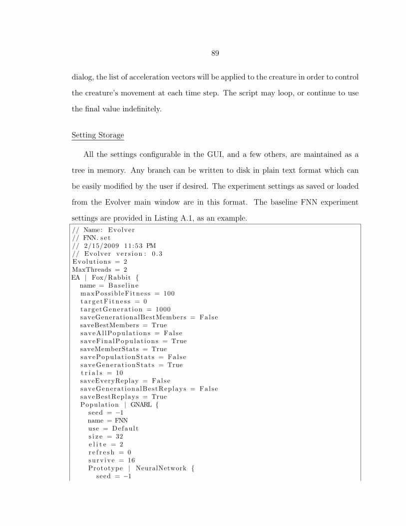
89
dialog, the list of acceleration vectors will be applied to the creature in order to control
the creature’s movement at each time step. The script may loop, or continue to use
the final value indefinitely.
Setting Storage
All the settings configurable in the GUI, and a few others, are maintained as a
tree in memory. Any branch can be written to disk in plain text format which can
be easily modified by the user if desired. The experiment settings as saved or loaded
from the Evolver main window are in this format. The baseline FNN experiment
settings are provided in Listing A.1, as an example.
// Name : Evolver// FNN. s e t// 2/15/2009 11 :53 PM// Evolver ve r s i on : 0 . 3Evo lut ions = 2MaxThreads = 2EA | Fox/Rabbit {
name = Base l i n emaxPoss ib l eFi tness = 100t a r g e tF i t n e s s = 0targetGenerat ion = 1000saveGenerationalBestMembers = FalsesaveBestMembers = TruesaveAl lPopu la t i ons = FalsesaveF ina lPopu la t i ons = TruesaveMemberStats = TruesavePopu lat ionStat s = FalsesaveGenerat ionStats = Truet r i a l s = 10saveEveryReplay = FalsesaveGenerat iona lBestReplays = FalsesaveBestReplays = TruePopulat ion | GNARL {
seed = −1name = FNNuse = Defau l ts i z e = 32e l i t e = 2r e f r e s h = 0surv ive = 16Prototype | NeuralNetwork {
seed = −1
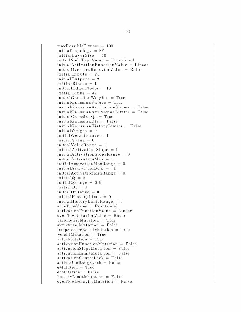
90
maxPoss ib leFi tness = 100i n i t i a lTopo l o gy = FFi n i t i a l L a y e r S i z e = 10in it ia lNodeTypeValue = Frac t i ona li n i t i a lAc t i va t i onFunc t i onVa lu e = Linearin i t i a lOve r f l owBehav io rVa lue = Ratioi n i t i a l I n p u t s = 24i n i t i a lOu tpu t s = 2i n i t i a l B i a s e s = 1in i t i a lH iddenNodes = 10i n i t i a l L i n k s = 42in i t i a lGaus s i anWe ight s = Truei n i t i a lGau s s i anVa lu e s = Truei n i t i a lGau s s i a nAc t i v a t i o nS l op e s = Falsei n i t i a lGau s s i anAc t i v a t i onL im i t s = Falsei n i t i a lGaus s i anQs = Truei n i t i a lGau s s i anDt s = Falsei n i t i a lGau s s i anH i s t o r yL im i t s = Falsei n i t i a lWe i gh t = 0in i t ia lWeightRange = 1i n i t i a lV a l u e = 0in i t i a lVa lueRange = 1i n i t i a lA c t i v a t i o n S l o p e = 1in i t i a lAc t i v a t i onS l opeRange = 0in i t i a lAc t i va t i onMax = 1in i t ia lAct ivat ionMaxRange = 0i n i t i a lAc t i v a t i onMin = −1in i t i a lAct ivat i onMinRange = 0i n i t i a lQ = 0in i t ia lQRange = 0 .5i n i t i a l D t = 1in i t i a lDtRange = 0i n i t i a lH i s t o r yL im i t = 0in i t i a lH i s t o ryL im i tRange = 0nodeTypeValue = Frac t i ona lact ivat ionFunct ionValue = Linearover f lowBehaviorValue = RatioparametricMutation = Trues t ruc tura lMutat ion = FalsetemperatureBasedMutation = TrueweightMutation = TruevalueMutation = Trueact ivat ionFunct ionMutat ion = Falseact ivat ionS lopeMutat ion = Falseact ivat ionLimitMutat ion = Falseact ivat ionCenterLock = Falseact ivat ionRangeLock = FalseqMutation = TruedtMutation = Falseh i s toryLimitMutat ion = Falseoverf lowBehaviorMutat ion = False
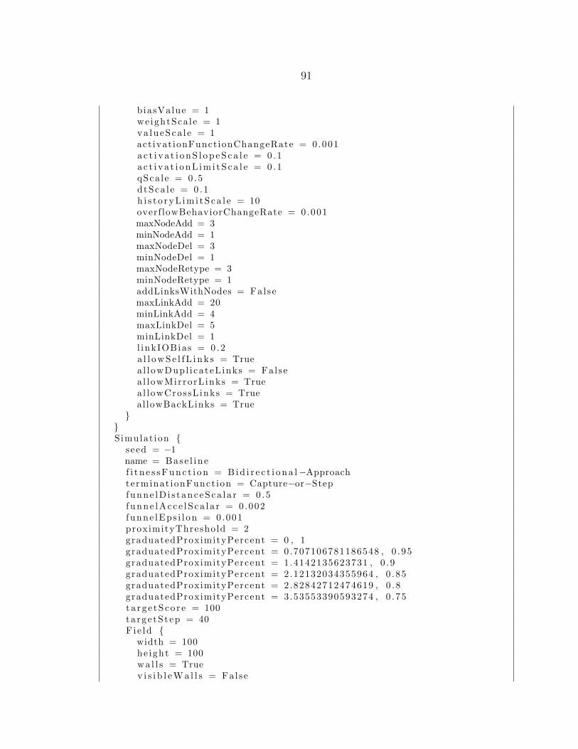
91
biasValue = 1we ightSca l e = 1va lueSca l e = 1act ivat ionFunct ionChangeRate = 0.001a c t i v a t i onS l op eS c a l e = 0 .1a c t i v a t i onL im i tS ca l e = 0 .1qSca le = 0 .5dtSca l e = 0 .1h i s t o ryL im i tS ca l e = 10overf lowBehaviorChangeRate = 0.001maxNodeAdd = 3minNodeAdd = 1maxNodeDel = 3minNodeDel = 1maxNodeRetype = 3minNodeRetype = 1addLinksWithNodes = FalsemaxLinkAdd = 20minLinkAdd = 4maxLinkDel = 5minLinkDel = 1l inkIOBias = 0 .2a l l owSe l fL i nk s = Truea l l owDupl i ca teL inks = Falsea l lowMirrorL inks = Truea l lowCrossL inks = Trueal lowBackLinks = True
}}Simulat ion {
seed = −1name = Base l i n ef i t n e s sFunc t i on = B id i r e c t i o na l−Approachterminat ionFunct ion = Capture−or−Stepfunne lD i s t anceSca l a r = 0 .5funne lAcc e lS ca l a r = 0.002funne lEps i l on = 0.001proximityThreshold = 2graduatedProximityPercent = 0 , 1graduatedProximityPercent = 0.707106781186548 , 0 .95graduatedProximityPercent = 1.4142135623731 , 0 . 9graduatedProximityPercent = 2.12132034355964 , 0 .85graduatedProximityPercent = 2.82842712474619 , 0 . 8graduatedProximityPercent = 3.53553390593274 , 0 .75ta rg e tSco r e = 100ta rge tStep = 40F ie ld {
width = 100he ight = 100wa l l s = Truev i s i b l eWa l l s = Fal se

92
}Fox | NeuralNetwork {
seed = −1rad iu s = 0 .5startAnywhere = Falses t a r t = 0 , 0startRange = 0 , 0s t a r tD i s t anc e = 49startAzimuth = 0startAzimuthRange = 180maxSpeed = 5maxAccel = 1ve loc i tyDecayRate = 0 .1r o l e = FoxsensorCount = 12sen so rReso lu t i on = 30resetNetwork = TrueBrain {
NN 0} data
}Rabbit | Stat i onary {
seed = −1rad iu s = 0 .5startAnywhere = Falses t a r t = 0 , 0startRange = 0 , 0s t a r tD i s t anc e = 0startAzimuth = 0startAzimuthRange = 180maxSpeed = 5maxAccel = 1ve loc i tyDecayRate = 0 .1r o l e = RabbitsensorCount = 12sen so rReso lu t i on = 30
}}
}
Listing A.1: Baseline FNN.set
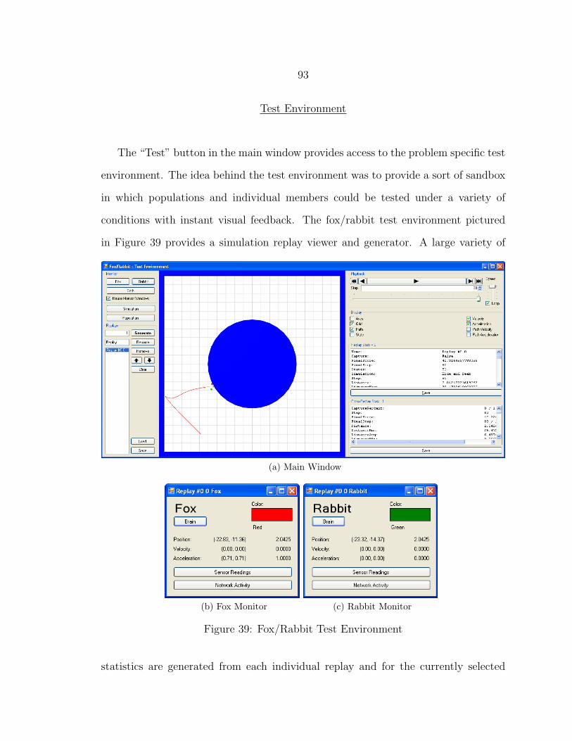
93
Test Environment
The “Test” button in the main window provides access to the problem specific test
environment. The idea behind the test environment was to provide a sort of sandbox
in which populations and individual members could be tested under a variety of
conditions with instant visual feedback. The fox/rabbit test environment pictured
in Figure 39 provides a simulation replay viewer and generator. A large variety of
(a) Main Window
(b) Fox Monitor (c) Rabbit Monitor
Figure 39: Fox/Rabbit Test Environment
statistics are generated from each individual replay and for the currently selected

94
group of replays in the two panes to the lower right. Step by step traversal of replays
is provided as well as automated playback at adjustable speed. The “Simulation”
button opens the simulation settings dialog from Figure 34 as it applies to the local
test environment simulation. All settings provided by its subtree of dialogs are also
adjustable. The “Population” button similarly opens the population edit dialog from
Figure 29. This controls a population of members local to the test environment which
can be used to generate simulation replays for playback and observation of statistics.
The field to the left of the “Generate” button controls the number of replays generated
for each member of the population when the button is activated.
Each of the creature monitors shown in Figures 39b and 39c update with the
corresponding creature’s movement as the main test environment window plays back
the selected replay. These monitor windows also provide access to “Sensor Readings”
and “Network Activity” for the creature they represent. Figure 40a shows the sensor
readings corresponding to the state of the test environment in Figure 39a. The
information in the sensor readings window updates according to mouse-over input
and as the replay state changes in the main test environment window. Each pair of
vertically stacked colored blocks in the top half of the window represents one sensor.
It is shaded according to the value reported by the sensor. Blue represents walls and
obstacles, while red represents other creatures. The intensity values are greyscale.
Similarly, each pair of much narrower stacked color bars in the bottom half of the
window represents a sensor cell. Figure 40b displays the values of the nodes and links
in the creature’s “Brain”. This data also updates according to mouse-over input and
to track replay state changes in the main test environment window. The colored
squares arranged in a grid in the top section of the window represent the nodes of
the network in internally indexed order. These are shaded to match their activation
values. The activation value of an input or bias node is simply its value, while the
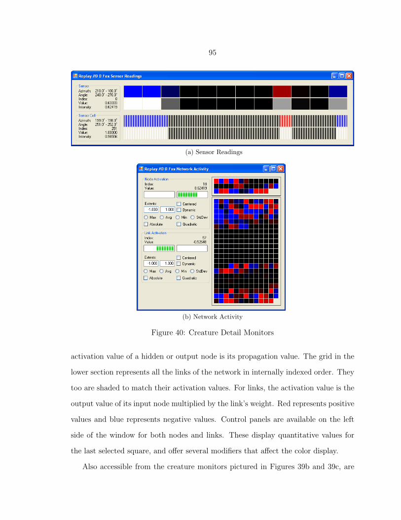
95
(a) Sensor Readings
(b) Network Activity
Figure 40: Creature Detail Monitors
activation value of a hidden or output node is its propagation value. The grid in the
lower section represents all the links of the network in internally indexed order. They
too are shaded to match their activation values. For links, the activation value is the
output value of its input node multiplied by the link’s weight. Red represents positive
values and blue represents negative values. Control panels are available on the left
side of the window for both nodes and links. These display quantitative values for
the last selected square, and offer several modifiers that affect the color display.
Also accessible from the creature monitors pictured in Figures 39b and 39c, are
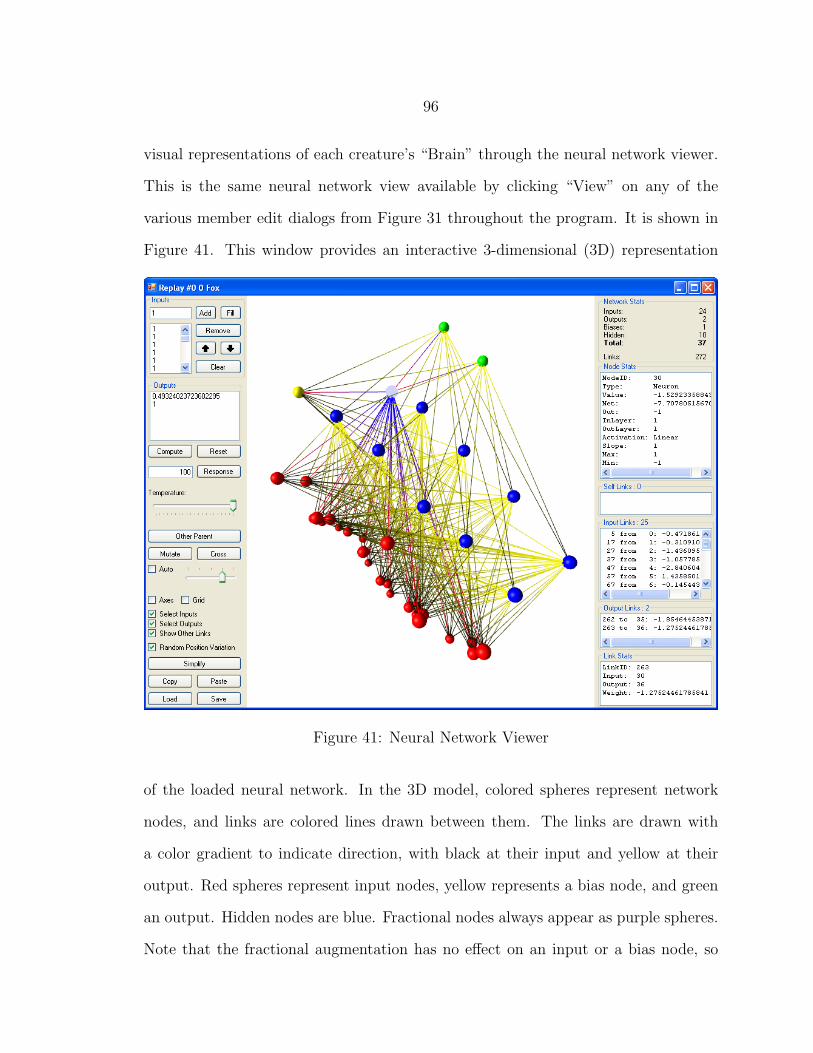
96
visual representations of each creature’s “Brain” through the neural network viewer.
This is the same neural network view available by clicking “View” on any of the
various member edit dialogs from Figure 31 throughout the program. It is shown in
Figure 41. This window provides an interactive 3-dimensional (3D) representation
Figure 41: Neural Network Viewer
of the loaded neural network. In the 3D model, colored spheres represent network
nodes, and links are colored lines drawn between them. The links are drawn with
a color gradient to indicate direction, with black at their input and yellow at their
output. Red spheres represent input nodes, yellow represents a bias node, and green
an output. Hidden nodes are blue. Fractional nodes always appear as purple spheres.
Note that the fractional augmentation has no effect on an input or a bias node, so

97
those node types cannot be changed. When a node is selected, it is lightened in color
and enlarged. Its incident links may also be selected depending on user specified
options. When a link is selected it changes to a red–blue gradient with blue at the
output.
The right side of the window provides basic network component counts and state
information for the currently selected node and its links. The primary purpose of
the neural network viewer was to allow a neural network to be inspected visually, to
ensure that the user’s concept of the network matched the program’s model.
The upper left section of the window allows inputs to be specified. The resulting
outputs are then displayed when computed. The “Reset” button clears any state
information in the network to allow for fresh computation. The field to the left of the
“Response” button specifies how many compute cycles are run and stored to disk when
the button is clicked. Below these controls is a set of controls for testing mutation
and crossover operations. The “Other Parent” button opens a dialog similar to the
one in Figure 31 which allows another network to be loaded for crossover testing.
The temperature slider naturally controls the instantaneous temperature value for
mutation. The “Mutate” and “Cross” buttons apply the mutation or crossover
operations respectively. If the “Auto” box is checked, these will toggle the automatic
application of the corresponding operator at a rate controlled by the slider to its right.
The “Simplify” button prunes nodes and links from the network which are not in the
computation path.
Statistic Aggregation
The layered approach to statistic aggregation described in the “Statistic Collec-
tion” section at the end of Chapter 3 was done with the help of self merging lists

98
of statistic objects. Each relevant quantity was assigned a name and added to the
statistic list at the appropriate level. Transfer of these statistics to higher levels was
done using functions that automatically expanded each statistic object in the list into
a group of statistic objects where each represented a component of the previous level
statistic. A long list of named quantities (115,415 for the current version of Evolver)
resulted at the final level of aggregation. Logging options were used to select which
levels of statistics were written to disk.
A separate program was written to aggregate the statistic data output from
multiple evolutions. This provided the convenience of running discontinuous
evolutions by parts, possibly even on multiple host computers while still allowing
for easily acquired experiment level statistics.

99
Appendix B
CODE LISTINGS
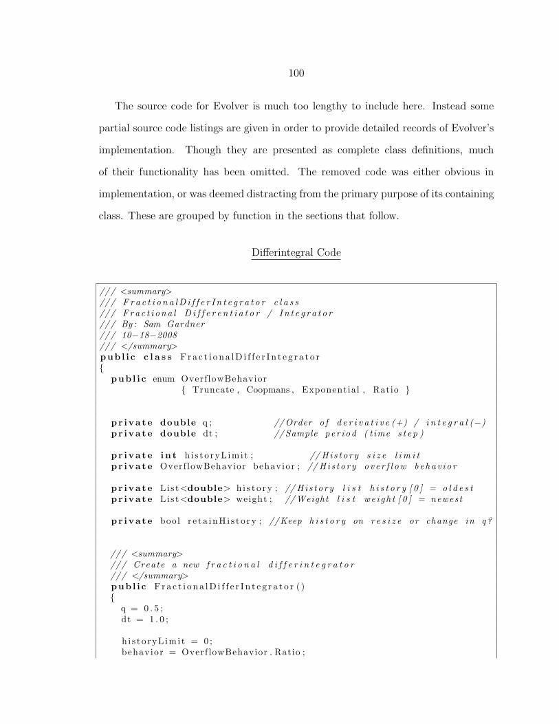
100
The source code for Evolver is much too lengthy to include here. Instead some
partial source code listings are given in order to provide detailed records of Evolver’s
implementation. Though they are presented as complete class definitions, much
of their functionality has been omitted. The removed code was either obvious in
implementation, or was deemed distracting from the primary purpose of its containing
class. These are grouped by function in the sections that follow.
Differintegral Code
/// <summary>/// F r a c t i o n a lD i f f e r I n t e g r a t o r c l a s s/// Fra c t i ona l D i f f e r e n t i a t o r / I n t e g r a t o r/// By : Sam Gardner/// 10−18−2008/// </summary>pub l i c c l a s s Fr a c t i o n a lD i f f e r I n t e g r a t o r{
pub l i c enum Overf lowBehavior{ Truncate , Coopmans , Exponential , Ratio }
pr i va t e double q ; //Order o f d e r i v a t i v e (+) / i n t e g r a l (−)pr i va t e double dt ; //Sample pe r i od ( t ime s t e p )
pr i va t e i n t h i s t o ryL im i t ; // Hi s t o ry s i z e l i m i tpr i va t e Overf lowBehavior behavior ; // Hi s t o ry o v e r f l ow behav i o r
pr i va t e List<double> h i s t o r y ; // Hi s t o ry l i s t h i s t o r y [ 0 ] = o l d e s tpr i va t e List<double> weight ; //Weight l i s t we i gh t [ 0 ] = newest
pr i va t e bool r e t a i nH i s t o r y ; //Keep h i s t o r y on r e s i z e or change in q?
/// <summary>/// Create a new f r a c t i o n a l d i f f e r i n t e g r a t o r/// </summary>pub l i c Fr a c t i o n a lD i f f e r I n t e g r a t o r ( ){
q = 0 . 5 ;dt = 1 . 0 ;
h i s t o ryL im i t = 0 ;behavior = Overf lowBehavior . Ratio ;
101
h i s t o r y = new List<double >() ;weight = new List<double >() ;
r e t a i nH i s t o r y = true ;
CalcWeights ( ) ;}
/// <summary>/// Provide the nex t sample to the d i f f e r i n t e g r a l/// <para>The r e s u l t i n g d i f f e r i n t e g r a l i s re turned </para>/// <para>/// Prov id ing i npu t s a t i n t e r v a l s o t h e r than Dt/// may i n v a l i d a t e r e s u l t s/// </para>/// </summary>/// <param name=”va l u e”>nex t inpu t sample</param>pub l i c double Compute ( double value ){
I n s e r t ( va lue ) ;return Compute ( h i s t o r y ) ;
}
/// <summary>/// Return the d i f f e r i n t e g r a l f o r a prov ided h i s t o r y/// The prov ided v a l u e s are not added to the i n t e r n a l h i s t o r y/// </summary>/// <param name=”curve”> l i s t o f h i s t o r y va lue s </param>pub l i c double Compute ( Lis t<double> curve ){
double sum = 0 . 0 ;i n t idx ;i n t i ;
f o r ( i = 0 ; i < curve . Count ; i++){
idx = curve . Count − 1 − i ;i f ( i > weight . Count − 1) CalcWeights ( ) ;sum += curve [ idx ] ∗ weight [ i ] ;
}
return sum / Math .Pow( dt , q ) ;}
/// <summary>/// Add a sample va l u e to the h i s t o r y/// </summary>/// <param name=”va l u e”>nex t inpu t sample</param>pub l i c void I n s e r t ( double value ){

102
i f ( h i s t o ryL im i t != 0 && h i s t o r y . Count >= hi s to ryL imi t ){
switch ( behavior ){
case Overf lowBehavior . Ratio :double r ;
i f ( weight . Count < h i s t o r y . Count ) CalcWeights ( ) ;i f ( h i s t o r y . Count < 2)
r = 0 . 9 9 ;e l s e
r = weight [ h i s t o r y . Count − 1 ] / weight [ h i s t o r y . Count − 2 ] ;
h i s t o r y [ 1 ] += h i s t o r y [ 0 ] ∗ r ;break ;
case Overf lowBehavior . Exponent ia l :h i s t o r y [ 1 ] += h i s t o r y [ 0 ] ∗ 0 . 9 9 ;break ;
case Overf lowBehavior . Coopmans :i f ( weight . Count < h i s t o r y . Count ) CalcWeights ( ) ;va lue += h i s t o r y [ 0 ] ∗ weight [ h i s t o r y . Count − 1 ] ;break ;
de f au l t : // Over f lowBehav ior . Truncatebreak ;
}
h i s t o r y . RemoveAt ( 0 ) ;}
h i s t o r y .Add( value ) ;}
/// <summary>/// Ca l c u l a t e and s t o r e the nex t uncomputed we i gh t/// </summary>pr i va t e void NextWeight ( ){
i n t k = weight . Count ;
i f ( k == 0)weight .Add ( 1 . 0 ) ;
e l s eweight .Add( weight [ k − 1 ] ∗ ( k − 1 − q ) / k ) ;
}
/// <summary>/// Ca l c u l a t e enough we i g h t s to d i f f e r i n t e g r a t e/// over the e n t i r e i n t e r n a l h i s t o r y

103
/// </summary>pub l i c void CalcWeights ( ){
CalcWeights (Math .Max( h i s t o r y . Count , h i s t o ryL im i t ) ) ;}
/// <summary>/// Ca l c u l a t e enough we i g h t s to d i f f e r i n t e g r a t e over/// a h i s t o r y o f t h e s p e c i f i e d l e n g t h/// </summary>/// <param name=” l e n g t h”>h i s t o r y l eng th </param>pub l i c void CalcWeights ( i n t l ength ){
whi le ( weight . Count < l ength )NextWeight ( ) ;
}}
Listing B.1: Selections from FractionalDifferIntegrator.cs
Neural Network Code
/// <summary>/// Neuron c l a s s/// By : Sam Gardner/// 10−31−2007/// Modi f i ed : 02−15−2009/// </summary>pub l i c c l a s s Neuron : IEnumerable<Neuron>{
pub l i c const s t r i n g DEFAULT TYPE = ”Neuron” ;pub l i c const double DEFAULT VALUE = 0 . 0 ;pub l i c const s t r i n g DEFAULT ACTIVATION FUNCTION = ”Tanh” ;pub l i c const double DEFAULT ACTIVATION SLOPE = 1 . 0 ;pub l i c const double DEFAULT MAX ACTIVATION VALUE = 1 . 0 ;pub l i c const double DEFAULT MIN ACTIVATION VALUE = −1.0;
protected List<double> inWeight ; // Weights o f incoming l i n k sprotected List<Neuron> inLink ; // Incoming l i n k s from o the r nodesprotected List<Neuron> outLink ; // Outgoing l i n k s to o t h e r nodes
protected s t r i n g actFunc ; // Ac t i v a t i on f un c t i on type nameprotected double actS lope ; // Ac t i v a t i on s l o p eprotected double maxActValue ; // Maximum a c t i v a t i o n ou tpu t va l u eprotected double minActValue ; // Minimum a c t i v a t i o n ou tpu t va l u e
protected double value ; // Value o f neuron
104
protected double propValue ; // Propagat ion va l u eprotected double auxValue ; // Aux i l l a r y computat ion va l u eprotected double output ; // Output va l u e
protected i n t inLayer ; // Layer index from inpu tprotected i n t outLayer ; // Layer index from outpu t
protected bool computed ; // Computed f l a gprotected bool v i s i t e d ; // V i s i t e d f l a g
/// <summary>/// Create a new neuron/// </summary>pub l i c Neuron ( ){
inWeight = new List<double >() ;inLink = new List<Neuron >() ;outLink = new List<Neuron >() ;
actFunc = DEFAULT ACTIVATION FUNCTION;actS lope = DEFAULT ACTIVATION SLOPE;maxActValue = DEFAULT MAX ACTIVATION VALUE;minActValue = DEFAULT MIN ACTIVATION VALUE;
value = DEFAULT VALUE;propValue = 0 . 0 ;auxValue = 0 . 0 ;output = double .NaN;
inLayer = −1;outLayer = −1;
computed = f a l s e ;v i s i t e d = f a l s e ;
}
/// <summary>/// Traverse t h i s node s e t t i n g v i s i t e d f l a g s/// </summary>pub l i c v i r t u a l void Traverse ( ){
i f ( ! v i s i t e d ){
v i s i t e d = true ;
f o r each (Neuron i in inLink )i . Traverse ( ) ;
}}
105
/// <summary>/// I n i t i a l i z e t h i s neuron between uses/// <para>/// Intended to c l e a r s t a t e memory and o the r f e a t u r e s which/// shou l d not be c a r r i e d over between prob lems/// </para>/// </summary>pub l i c v i r t u a l void I n i t i a l i z e ( ){
propValue = 0 . 0 ;auxValue = 0 . 0 ;output = double .NaN;
Reset ( ) ;}
/// <summary>/// Reset t h i s neuron f o r another computat ion/// </summary>pub l i c void Reset ( ){
computed = f a l s e ;v i s i t e d = f a l s e ;
}
/// <summary>/// Return or compute the ou tpu t va l u e o f t h i s neuron/// <para>/// Designed f o r r e c u r s i v e computat ion s t a r t i n g a t network ou t pu t s/// </para>/// </summary>/// <re turns >neuron output </re turns >pub l i c v i r t u a l double Compute ( ){
i f ( ! computed ){
i f ( v i s i t e d )return PrematureOutput ( ) ;
v i s i t e d = true ;
// Don ’ t a d j u s t t he va l u e o f i npu t and b i a s nodesi f ( inLink . Count <= 0){
propValue = value ;auxValue = value ;output = value ;
}e l s e{
propValue = Propagation ( ) ;
106
auxValue = Aux i l l a ry ( propValue ) ;output = Act ivat ion ( auxValue ) ;
}
computed = true ;}
return output ;}
/// <summary>/// Return an ou tpu t va l u e premature l y/// <para>/// This i s r e qu i r e d when a c y c l e i s encountered in the network/// Some i n i t i a l v a l u e i s r e q u i r e d to unwrap the c y c l e/// </para>/// </summary>/// <re turns >a premature ou tpu t f o r t h i s neuron</re turns >pub l i c v i r t u a l double PrematureOutput ( ){
i f ( inLink . Count <= 0){
propValue = value ;auxValue = value ;output = value ;
}e l s e i f ( double . IsNaN( output ) ){
propValue = value ;auxValue = Aux i l l a ry ( propValue ) ;output = Act ivat ion ( auxValue ) ;
}
return output ;}
/// <summary>/// Compute the propaga t i on va l u e f o r t h i s neuron/// <para>Input and Bias nodes r e tu rn 0.0</para>/// </summary>pub l i c v i r t u a l double Propagation ( ){
// Compute we i gh t ed sum o f i npu t sdouble net = 0 . 0 ;f o r ( i n t n = 0 ; n < inLink . Count ; n++)
net += inLink [ n ] . Compute ( ) ∗ inWeight [ n ] ;
return net ;}
/// <summary>
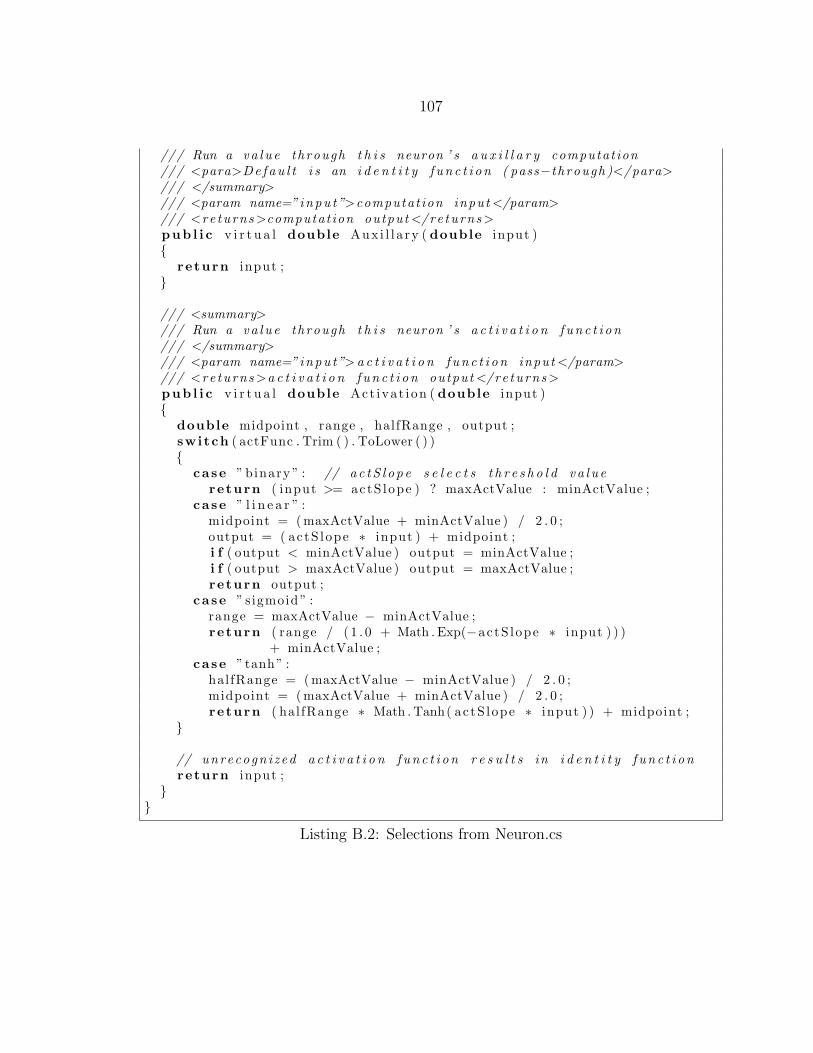
107
/// Run a va l u e through t h i s neuron ’ s a u x i l l a r y computat ion/// <para>De fau l t i s an i d e n t i t y f un c t i on ( pass−through )</para>/// </summary>/// <param name=”inpu t”>computat ion input </param>/// <re turns >computat ion output </re turns >pub l i c v i r t u a l double Aux i l l a ry ( double input ){
return input ;}
/// <summary>/// Run a va l u e through t h i s neuron ’ s a c t i v a t i o n f un c t i on/// </summary>/// <param name=”inpu t”>a c t i v a t i o n f un c t i on input </param>/// <re turns >a c t i v a t i o n f un c t i on output </re turns >pub l i c v i r t u a l double Act ivat ion ( double input ){
double midpoint , range , halfRange , output ;switch ( actFunc . Trim ( ) . ToLower ( ) ){
case ” binary ” : // ac tS l o p e s e l e c t s t h r e s h o l d va l u ereturn ( input >= actS lope ) ? maxActValue : minActValue ;
case ” l i n e a r ” :midpoint = (maxActValue + minActValue ) / 2 . 0 ;output = ( actS lope ∗ input ) + midpoint ;i f ( output < minActValue ) output = minActValue ;i f ( output > maxActValue ) output = maxActValue ;return output ;
case ” sigmoid ” :range = maxActValue − minActValue ;return ( range / ( 1 . 0 + Math . Exp(−actS lope ∗ input ) ) )
+ minActValue ;case ”tanh” :
halfRange = (maxActValue − minActValue ) / 2 . 0 ;midpoint = (maxActValue + minActValue ) / 2 . 0 ;return ( halfRange ∗ Math . Tanh( actS lope ∗ input ) ) + midpoint ;
}
// unrecogn i z ed a c t i v a t i o n f un c t i on r e s u l t s in i d e n t i t y f un c t i onreturn input ;
}}
Listing B.2: Selections from Neuron.cs
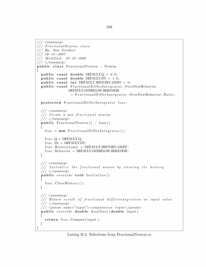
108
/// <summary>/// Fract iona lNeuron c l a s s/// By : Sam Gardner/// 10−31−2007/// Modi f i ed : 10−22−2008/// </summary>pub l i c c l a s s Fract ionalNeuron : Neuron{
pub l i c const double DEFAULT Q = 0 . 0 ;pub l i c const double DEFAULT DT = 1 . 0 ;pub l i c const i n t DEFAULT HISTORY LIMIT = 0 ;pub l i c const Fr a c t i o n a lD i f f e r I n t e g r a t o r . Overf lowBehavior
DEFAULT OVERFLOW BEHAVIOR= Fra c t i o n a lD i f f e r I n t e g r a t o r . Overf lowBehavior . Ratio ;
protected Fr a c t i o n a lD i f f e r I n t e g r a t o r f r a c ;
/// <summary>/// Create a new f r a c t i o n a l neuron/// </summary>pub l i c Fract ionalNeuron ( ) : base ( ){
f r a c = new Fr a c t i o n a lD i f f e r I n t e g r a t o r ( ) ;
f r a c .Q = DEFAULT Q;f r a c . Dt = DEFAULT DT;f r a c . His toryLimit = DEFAULT HISTORY LIMIT;f r a c . Behavior = DEFAULT OVERFLOW BEHAVIOR;
}
/// <summary>/// I n i t i a l i z e t he f r a c t i o n a l neuron by c l e a r i n g i t s h i s t o r y/// </summary>pub l i c ove r r i d e void I n i t i a l i z e ( ){
f r a c . C learHi s tory ( ) ;}
/// <summary>/// Return r e s u l t o f f r a c t i o n a l d i f f e r i n t e g r a t i o n on inpu t va l u e/// </summary>/// <param name=”inpu t”>computat ion input </param>pub l i c ove r r i d e double Aux i l l a ry ( double input ){
return f r a c . Compute ( input ) ;}
}
Listing B.3: Selections from FractionalNeuron.cs

109
/// <summary>/// NeuralNetwork c l a s s/// By : Sam Gardner/// 10−31−2007/// Modi f i ed : 12−16−2008/// </summary>pub l i c c l a s s NeuralNetwork : IEnumerable<Neuron>{
protected RandomGenerator rand ;
protected List<Neuron> node ; // A l l neurons in networkprotected List<Neuron> inputNode ; // A l l i npu t neurons in networkprotected List<Neuron> outputNode ; // A l l ou tpu t neurons in network
/// <summary>/// Create a new neura l network/// </summary>pub l i c NeuralNetwork ( ){
rand = new RandomGenerator ( ) ;
node = new List<Neuron >() ;inputNode = new List<Neuron >() ;outputNode = new List<Neuron >() ;
}
/// <summary>/// Create a neura l network by copy ing another/// </summary>/// <param name=”nn”>neura l network to copy</param>pub l i c NeuralNetwork ( NeuralNetwork nn){
i n t index ;
rand = nn . rand . Copy ( ) ;
node = new List<Neuron >() ;inputNode = new List<Neuron >() ;outputNode = new List<Neuron >() ;
f o r each (Neuron n in nn . node )node .Add(n . Copy ( ) ) ;
f o r ( i n t n = 0 ; n < nn . node . Count ; n++)f o r ( i n t i = 0 ; i < nn . node [ n ] . InputCount ; i++){
index = nn . node . IndexOf (nn . node [ n ] . Input ( i ) ) ;node [ n ] . AddInput ( node [ index ] , nn . node [ n ] . Weight ( i ) ) ;
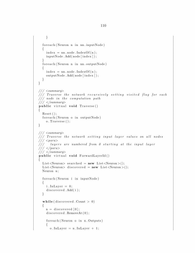
110
}
f o r each (Neuron n in nn . inputNode ){
index = nn . node . IndexOf (n ) ;inputNode .Add( node [ index ] ) ;
}f o r each (Neuron n in nn . outputNode ){
index = nn . node . IndexOf (n ) ;outputNode .Add( node [ index ] ) ;
}}
/// <summary>/// Traverse the network r e c u r s i v e l y s e t t i n g v i s i t e d f l a g f o r each/// node in the computat ion path/// </summary>pub l i c v i r t u a l void Traverse ( ){
Reset ( ) ;f o r each (Neuron o in outputNode )
o . Traverse ( ) ;}
/// <summary>/// Traverse the network s e t t i n g inpu t l a y e r v a l u e s on a l l nodes/// <para>/// l a y e r s are numbered from 0 s t a r t i n g a t t he inpu t l a y e r/// </para>/// </summary>pub l i c v i r t u a l void ForwardLayerId ( ){
List<Neuron> searched = new List<Neuron >() ;L i s t<Neuron> d i s cove r ed = new List<Neuron >() ;Neuron n ;
f o r each (Neuron i in inputNode ){
i . InLayer = 0 ;d i s cove r ed .Add( i ) ;
}
whi le ( d i s cove r ed . Count > 0){
n = di s cove r ed [ 0 ] ;d i s cove r ed . RemoveAt ( 0 ) ;
f o r each (Neuron o in n . Outputs ){
o . InLayer = n . InLayer + 1 ;

111
i f ( ! searched . Contains ( o ) )d i s cove r ed .Add( o ) ;
}
searched .Add(n ) ;}
}
/// <summary>/// S imp l i f y neura l network by removing unused nodes/// </summary>pub l i c v i r t u a l void S imp l i f y ( ){
i n t i = 0 ;
Traverse ( ) ;
// Prune unused nodeswhi le ( i < node . Count ){
i f ( ! node [ i ] . V i s i t ed && ! inputNode . Contains ( node [ i ] ) &&! outputNode . Contains ( node [ i ] ) )
RemoveAt( i ) ;e l s e
i++;}
}
/// <summary>/// I n i t i a l i z e e n t i r e neura l network to b i r t h c ond i t i on/// <para>/// Intended to r e s e t s t a t e memory and o the r s t o r e d v a l u e s/// between prob lems/// </para>/// </summary>pub l i c v i r t u a l void I n i t i a l i z e ( ){
f o r each (Neuron n in node )n . I n i t i a l i z e ( ) ;
}
/// <summary>/// Reset neura l network node s t a t u s f o r another computat ion/// </summary>protected v i r t u a l void Reset ( ){
f o r each (Neuron n in node )n . Reset ( ) ;
}
/// <summary>
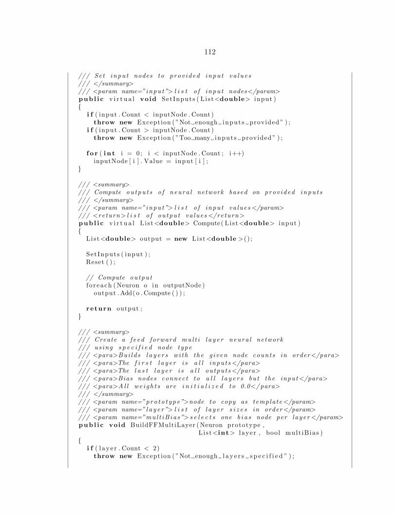
112
/// Set inpu t nodes to prov i ded inpu t v a l u e s/// </summary>/// <param name=”inpu t”> l i s t o f i npu t nodes</param>pub l i c v i r t u a l void SetInputs ( Li s t<double> input ){
i f ( input . Count < inputNode . Count )throw new Exception ( ”Not enough inputs provided ” ) ;
i f ( input . Count > inputNode . Count )throw new Exception ( ”Too many inputs provided ” ) ;
f o r ( i n t i = 0 ; i < inputNode . Count ; i++)inputNode [ i ] . Value = input [ i ] ;
}
/// <summary>/// Compute ou t pu t s o f neura l network based on prov ided i npu t s/// </summary>/// <param name=”inpu t”> l i s t o f i npu t va lue s </param>/// <re turn> l i s t o f ou tpu t va lue s </return>pub l i c v i r t u a l L i s t<double> Compute ( Lis t<double> input ){
List<double> output = new List<double >() ;
Set Inputs ( input ) ;Reset ( ) ;
// Compute ou tpu tf o r each (Neuron o in outputNode )
output .Add( o . Compute ( ) ) ;
return output ;}
/// <summary>/// Create a f e ed forward mu l t i l a y e r neura l network/// us ing s p e c i f i e d node type/// <para>Bui l d s l a y e r s w i th the g i v en node counts in order </para>/// <para>The f i r s t l a y e r i s a l l inpu t s </para>/// <para>The l a s t l a y e r i s a l l ou tpu t s </para>/// <para>Bias nodes connect to a l l l a y e r s bu t t he input </para>/// <para>Al l we i g h t s are i n i t i a l i z e d to 0.0</para>/// </summary>/// <param name=”pro t o t y p e”>node to copy as templa te </param>/// <param name=” l a y e r”> l i s t o f l a y e r s i z e s in order </param>/// <param name=”mu l t iB ia s”> s e l e c t s one b i a s node per l aye r </param>pub l i c void BuildFFMultiLayer (Neuron prototype ,
L i s t<int> l ayer , bool mult iBias ){
i f ( l a y e r . Count < 2)throw new Exception ( ”Not enough l a y e r s s p e c i f i e d ” ) ;
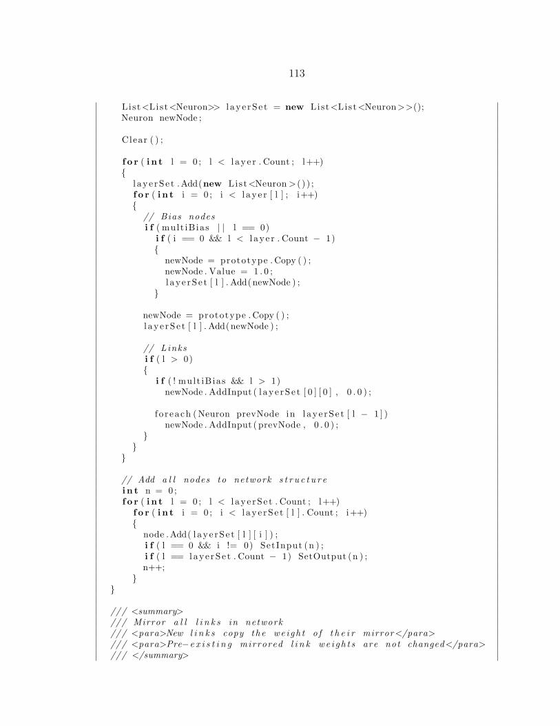
113
List<List<Neuron>> l a y e rS e t = new List<List<Neuron>>();Neuron newNode ;
Clear ( ) ;
f o r ( i n t l = 0 ; l < l a y e r . Count ; l++){
l a y e rS e t .Add(new List<Neuron > ( ) ) ;f o r ( i n t i = 0 ; i < l a y e r [ l ] ; i++){
// Bias nodesi f ( mult iBias | | l == 0)
i f ( i == 0 && l < l a y e r . Count − 1){
newNode = prototype . Copy ( ) ;newNode . Value = 1 . 0 ;l a y e rS e t [ l ] . Add(newNode ) ;
}
newNode = prototype . Copy ( ) ;l a y e rS e t [ l ] . Add(newNode ) ;
// Linksi f ( l > 0){
i f ( ! mult iBias && l > 1)newNode . AddInput ( l ay e rS e t [ 0 ] [ 0 ] , 0 . 0 ) ;
f o r each (Neuron prevNode in l ay e rS e t [ l − 1 ] )newNode . AddInput ( prevNode , 0 . 0 ) ;
}}
}
// Add a l l nodes to network s t r u c t u r ei n t n = 0 ;f o r ( i n t l = 0 ; l < l a y e rS e t . Count ; l++)
f o r ( i n t i = 0 ; i < l a y e rS e t [ l ] . Count ; i++){
node .Add( l ay e rS e t [ l ] [ i ] ) ;i f ( l == 0 && i != 0) SetInput (n ) ;i f ( l == laye rS e t . Count − 1) SetOutput (n ) ;n++;
}}
/// <summary>/// Mirror a l l l i n k s in network/// <para>New l i n k s copy the we i gh t o f t h e i r mirror </para>/// <para>Pre−e x i s t i n g mirrored l i n k we i g h t s are not changed</para>/// </summary>
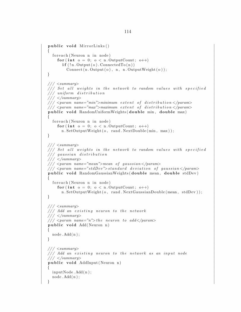
114
pub l i c void MirrorLinks ( ){
f o r each (Neuron n in node )f o r ( i n t o = 0 ; o < n . OutputCount ; o++)
i f ( ! n . Output ( o ) . ConnectedTo (n ) )Connect (n . Output ( o ) , n , n . OutputWeight ( o ) ) ;
}
/// <summary>/// Set a l l w e i g h t s in the network to random va l u e s wi th s p e c i f i e d/// uniform d i s t r i b u t i o n/// </summary>/// <param name=”min”>minimum ex t e n t o f d i s t r i b u t i o n </param>/// <param name=”max”>maximum ex t e n t o f d i s t r i b u t i o n </param>pub l i c void RandomUniformWeights ( double min , double max){
f o r each (Neuron n in node )f o r ( i n t o = 0 ; o < n . OutputCount ; o++)
n . SetOutputWeight ( o , rand . NextDouble (min , max ) ) ;}
/// <summary>/// Set a l l w e i g h t s in the network to random va l u e s wi th s p e c i f i e d/// gaus s i an d i s t r i b u t i o n/// </summary>/// <param name=”mean”>mean o f gauss ian </param>/// <param name=”stdDev”>s tandard d e v i a t i o n o f gauss ian </param>pub l i c void RandomGaussianWeights ( double mean , double stdDev ){
f o r each (Neuron n in node )f o r ( i n t o = 0 ; o < n . OutputCount ; o++)
n . SetOutputWeight ( o , rand . NextGaussianDouble (mean , stdDev ) ) ;}
/// <summary>/// Add an e x i s t i n g neuron to the network/// </summary>/// <param name=”n”> t h e neuron to add</param>pub l i c void Add(Neuron n){
node .Add(n ) ;}
/// <summary>/// Add an e x i s t i n g neuron to the network as an inpu t node/// </summary>pub l i c void AddInput (Neuron n){
inputNode .Add(n ) ;node .Add(n ) ;
}
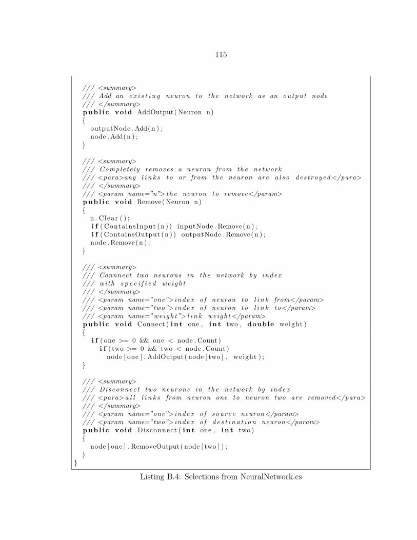
115
/// <summary>/// Add an e x i s t i n g neuron to the network as an ou tpu t node/// </summary>pub l i c void AddOutput (Neuron n){
outputNode .Add(n ) ;node .Add(n ) ;
}
/// <summary>/// Comple te ly removes a neuron from the network/// <para>any l i n k s to or from the neuron are a l s o des t royed </para>/// </summary>/// <param name=”n”> t h e neuron to remove</param>pub l i c void Remove(Neuron n){
n . Clear ( ) ;i f ( ContainsInput (n ) ) inputNode . Remove(n ) ;i f ( ContainsOutput (n ) ) outputNode . Remove(n ) ;node . Remove(n ) ;
}
/// <summary>/// Connnect two neurons in the network by index/// wi th s p e c i f i e d we i gh t/// </summary>/// <param name=”one”> index o f neuron to l i n k from</param>/// <param name=”two”> index o f neuron to l i n k to</param>/// <param name=”we i gh t”> l i n k weight </param>pub l i c void Connect ( i n t one , i n t two , double weight ){
i f ( one >= 0 && one < node . Count )i f ( two >= 0 && two < node . Count )
node [ one ] . AddOutput ( node [ two ] , weight ) ;}
/// <summary>/// Disconnect two neurons in the network by index/// <para>a l l l i n k s from neuron one to neuron two are removed</para>/// </summary>/// <param name=”one”> index o f source neuron</param>/// <param name=”two”> index o f d e s t i n a t i o n neuron</param>pub l i c void Disconnect ( i n t one , i n t two ){
node [ one ] . RemoveOutput ( node [ two ] ) ;}
}
Listing B.4: Selections from NeuralNetwork.cs
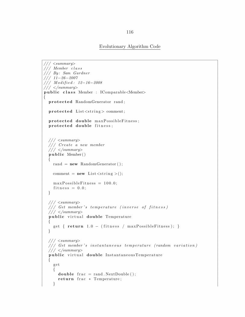
116
Evolutionary Algorithm Code
/// <summary>/// Member c l a s s/// By : Sam Gardner/// 11−26−2007/// Modi f i ed : 12−16−2008/// </summary>pub l i c c l a s s Member : IComparable<Member>{
protected RandomGenerator rand ;
protected List<s t r i ng > comment ;
protected double maxPoss ib l eFi tness ;protected double f i t n e s s ;
/// <summary>/// Create a new member/// </summary>pub l i c Member ( ){
rand = new RandomGenerator ( ) ;
comment = new List<s t r i ng >() ;
maxPoss ib leFi tness = 100 . 0 ;f i t n e s s = 0 . 0 ;
}
/// <summary>/// Get member ’ s t empera ture ( i n v e r s e o f f i t n e s s )/// </summary>pub l i c v i r t u a l double Temperature{
get { return 1 .0 − ( f i t n e s s / maxPoss ib leFi tness ) ; }}
/// <summary>/// Get member ’ s i n s t an t aneou s tempera ture ( random va r i a t i o n )/// </summary>pub l i c v i r t u a l double InstantaneousTemperature{
get{
double f r a c = rand . NextDouble ( ) ;return f r a c ∗ Temperature ;
}
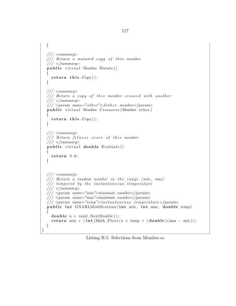
117
}
/// <summary>/// Return a mutated copy o f t h i s member/// </summary>pub l i c v i r t u a l Member Mutate ( ){
return t h i s . Copy ( ) ;}
/// <summary>/// Return a copy o f t h i s member c ro s s ed wi th another/// </summary>/// <param name=”o the r”> f a t h e r member</param>pub l i c v i r t u a l Member Crossover (Member other ){
return t h i s . Copy ( ) ;}
/// <summary>/// Return f i t n e s s s core o f t h i s member/// </summary>pub l i c v i r t u a l double Evaluate ( ){
return 0 . 0 ;}
/// <summary>/// Return a random number in the range [ min , max ]/// tempered by the in s t an t aneou s tempera ture/// </summary>/// <param name=”min”>minimum number</param>/// <param name=”max”>maximum number</param>/// <param name=”temp”> i n s t an t aneou s temperature </param>pub l i c i n t GNARLModifications ( i n t min , i n t max , double temp){
double u = rand . NextDouble ( ) ;return min + ( i n t )Math . Floor (u ∗ temp ∗ ( double ) (max − min ) ) ;
}}
Listing B.5: Selections from Member.cs
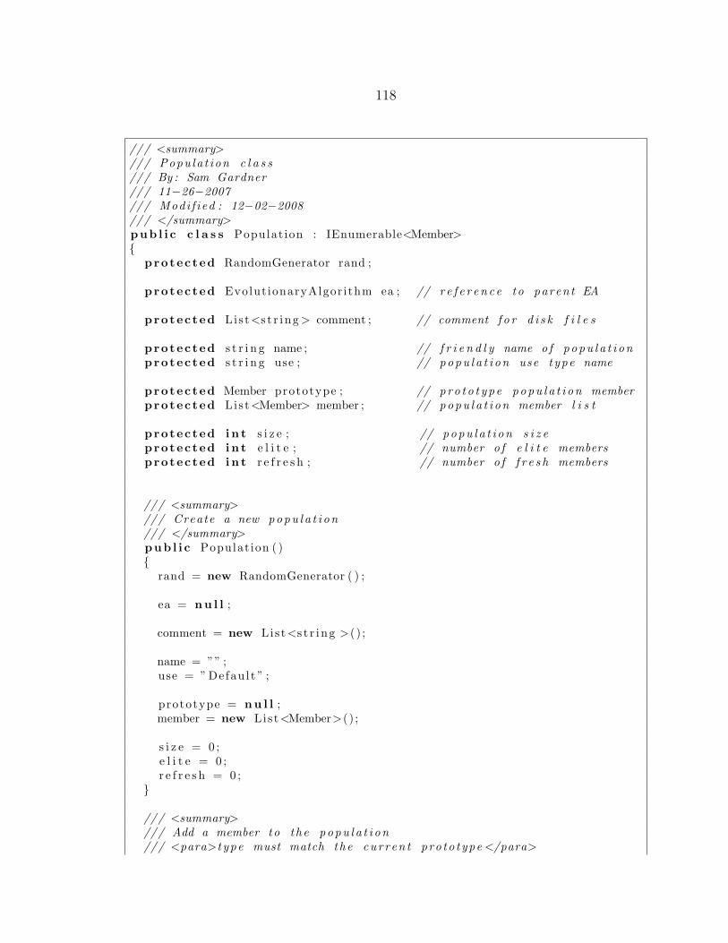
118
/// <summary>/// Popu la t ion c l a s s/// By : Sam Gardner/// 11−26−2007/// Modi f i ed : 12−02−2008/// </summary>pub l i c c l a s s Populat ion : IEnumerable<Member>{
protected RandomGenerator rand ;
protected Evolut ionaryAlgor ithm ea ; // r e f e r e n c e to parent EA
protected List<s t r i ng > comment ; // comment f o r d i s k f i l e s
protected s t r i n g name ; // f r i e n d l y name o f popu l a t i onprotected s t r i n g use ; // popu l a t i on use t ype name
protected Member prototype ; // p ro t o t y p e popu l a t i on memberprotected List<Member> member ; // popu l a t i on member l i s t
protected i n t s i z e ; // popu l a t i on s i z eprotected i n t e l i t e ; // number o f e l i t e membersprotected i n t r e f r e s h ; // number o f f r e s h members
/// <summary>/// Create a new popu l a t i on/// </summary>pub l i c Populat ion ( ){
rand = new RandomGenerator ( ) ;
ea = nu l l ;
comment = new List<s t r i ng >() ;
name = ”” ;use = ” Defau l t ” ;
prototype = nu l l ;member = new List<Member>() ;
s i z e = 0 ;e l i t e = 0 ;r e f r e s h = 0 ;
}
/// <summary>/// Add a member to the popu l a t i on/// <para>t ype must match the cur r en t pro to type </para>
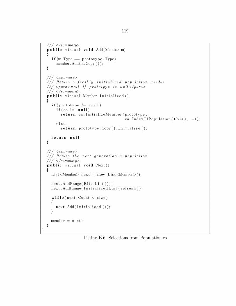
119
/// </summary>pub l i c v i r t u a l void Add(Member m){
i f (m. Type == prototype . Type )member .Add(m. Copy ( ) ) ;
}
/// <summary>/// Return a f r e s h l y i n i t i a l i z e d popu l a t i on member/// <para>n u l l i f p r o t o t y p e i s nu l l </para>/// </summary>pub l i c v i r t u a l Member I n i t i a l i z e d ( ){
i f ( prototype != nu l l )i f ( ea != nu l l )
return ea . In i t i a l i z eMember ( prototype ,ea . IndexOfPopulation ( t h i s ) , −1);
e l s ereturn prototype . Copy ( ) . I n i t i a l i z e ( ) ;
return nu l l ;}
/// <summary>/// Return the nex t g ene ra t i on ’ s popu l a t i on/// </summary>pub l i c v i r t u a l void Next ( ){
List<Member> next = new List<Member>() ;
next . AddRange( E l i t e L i s t ( ) ) ;next . AddRange( I n i t i a l i z e d L i s t ( r e f r e s h ) ) ;
whi le ( next . Count < s i z e ){
next .Add( I n i t i a l i z e d ( ) ) ;}
member = next ;}
}
Listing B.6: Selections from Population.cs

120
/// <summary>/// Evo lu t i onaryA l gor i t hm c l a s s/// By : Sam Gardner/// 11−24−2007/// Modi f i ed : 12−16−2008/// </summary>pub l i c c l a s s Evolut ionaryAlgor ithm{
protected s t r i n g name ;
protected List<s t r i ng > comment ;
protected List<Population> populat ion ;
protected i n t gene ra t i on ;protected bool i n i t i a l i z e d ;protected bool f i n i s h e d ;
protected double maxPoss ib l eFi tness ;
// Stopp ing Cond i t ionsprotected double t a r g e tF i t n e s s ;protected i n t ta rgetGenerat ion ;
// Reference to l o g and cur r en t s t a t e ( not cop i ed )protected EvolutionaryLog log ;protected Evolut ionaryState s t a t e ;
// Logging p r e f e r e n c e sprotected bool saveGenerationalBestMembers ;protected bool saveBestMembers ;
protected bool saveAl lPopu la t i ons ;protected bool saveF ina lPopu la t i ons ;
protected bool saveMemberStats ;protected bool savePopu lat ionStat s ;protected bool saveGenerat ionStats ;
/// <summary>/// Create a new e v o l u t i o n a r y a l g o r i t hm wi th no popu l a t i o n s/// </summary>pub l i c Evolut ionaryAlgor ithm ( ){
name = ”Evolut ion ” ;
comment = new List<s t r i ng >() ;
populat ion = new List<Population >() ;
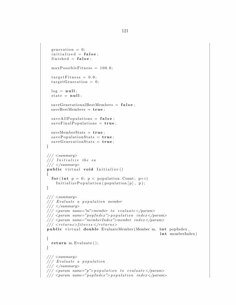
121
gene ra t i on = 0 ;i n i t i a l i z e d = f a l s e ;f i n i s h e d = f a l s e ;
maxPoss ib leFi tness = 100 . 0 ;
t a r g e tF i t n e s s = 0 . 0 ;ta rge tGenerat ion = 0 ;
l og = nu l l ;s t a t e = nu l l ;
saveGenerationalBestMembers = f a l s e ;saveBestMembers = true ;
s aveAl lPopu la t i ons = f a l s e ;s aveF ina lPopu la t i ons = true ;
saveMemberStats = true ;s avePopu lat ionStat s = true ;saveGenerat ionStats = true ;
}
/// <summary>/// I n i t i a l i z e t he ea/// </summary>pub l i c v i r t u a l void I n i t i a l i z e ( ){
f o r ( i n t p = 0 ; p < populat ion . Count ; p++)I n i t i a l i z eP o pu l a t i o n ( populat ion [ p ] , p ) ;
}
/// <summary>/// Eva lua te a popu l a t i on member/// </summary>/// <param name=”m”>member to e va l ua t e </param>/// <param name=”popIndex”>popu l a t i on index </param>/// <param name=”memberIndex”>member index </param>/// <re turns >f i t n e s s </re turns >pub l i c v i r t u a l double EvaluateMember (Member m, i n t popIndex ,
i n t memberIndex ){
return m. Evaluate ( ) ;}
/// <summary>/// Eva lua te a popu l a t i on/// </summary>/// <param name=”p”>popu l a t i on to eva l ua t e </param>/// <param name=”popIndex”>popu l a t i on index </param>

122
pub l i c v i r t u a l void EvaluatePopulat ion ( Populat ion p , i n t popIndex ){
f o r ( i n t m = 0 ; m < p . Count ; m++)p [m] . F i tne s s = EvaluateMember (p [m] , popIndex , m) ;
}
/// <summary>/// Eva lua te cur r en t g ene ra t i on/// </summary>pub l i c v i r t u a l void Evaluate ( ){
f o r ( i n t p = 0 ; p < populat ion . Count ; p++)EvaluatePopulat ion ( populat ion [ p ] , p ) ;
}
/// <summary>/// Adjus t a popu l a t i on member to o b t a i n a d i f f e r e n t one/// </summary>/// <param name=”m”>member to mutate</param>pub l i c v i r t u a l Member Mutate (Member m){
return m. Mutate ( ) ;}
/// <summary>/// Cross two popu l a t i on members to o b t a i n a new one r e l a t e d to bo th/// </summary>/// <param name=” f a t h e r ”> f a t h e r member</param>/// <param name=”mother”>mother member</param>pub l i c v i r t u a l Member Crossover (Member fa ther , Member mother ){
return mother . Crossover ( f a t h e r ) ;}
/// <summary>/// Generate nex t g ene ra t i on/// </summary>protected v i r t u a l void Next ( ){
f o r each ( Populat ion p in populat ion )p . Next ( ) ;
}
/// <summary>/// Reset ea f o r a new e v o l u t i o n/// </summary>pub l i c void Reset ( ){
i f ( l og != nu l l ) CreateNextState ( ) ;
g ene ra t i on = 0 ;
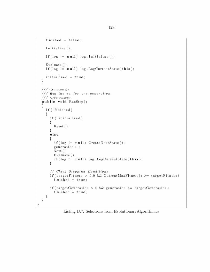
123
f i n i s h e d = f a l s e ;
I n i t i a l i z e ( ) ;
i f ( l og != nu l l ) l og . I n i t i a l i z e ( ) ;
Evaluate ( ) ;i f ( l og != nu l l ) l og . LogCurrentState ( t h i s ) ;
i n i t i a l i z e d = true ;}
/// <summary>/// Run the ea f o r one g ene ra t i on/// </summary>pub l i c void RunStep ( ){
i f ( ! f i n i s h e d ){
i f ( ! i n i t i a l i z e d ){
Reset ( ) ;}e l s e{
i f ( l og != nu l l ) CreateNextState ( ) ;g ene ra t i on++;Next ( ) ;Evaluate ( ) ;i f ( l og != nu l l ) l og . LogCurrentState ( t h i s ) ;
}
// Check S topp ing Cond i t i onsi f ( t a r g e tF i t n e s s > 0 .0 && CurrentMaxFitness ( ) >= ta r g e tF i t n e s s )
f i n i s h e d = true ;
i f ( ta rgetGenerat ion > 0 && genera t i on >= targetGenerat ion )f i n i s h e d = true ;
}}
}
Listing B.7: Selections from EvolutionaryAlgorithm.cs
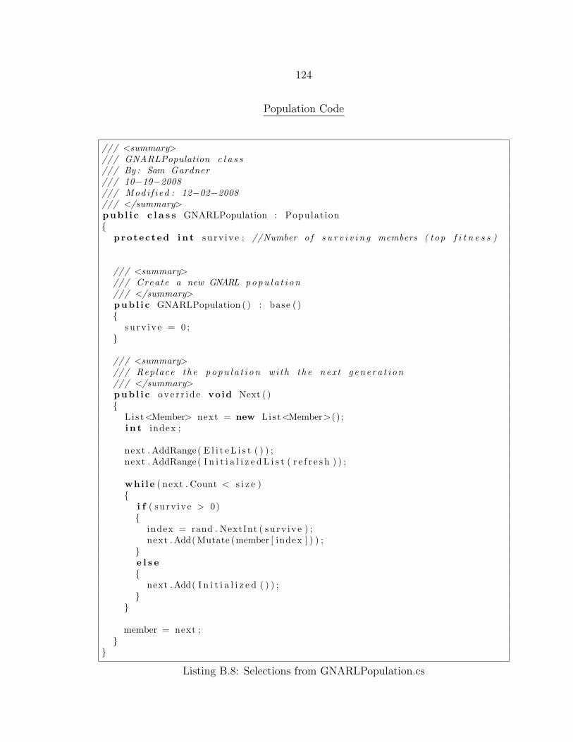
124
Population Code
/// <summary>/// GNARLPopulation c l a s s/// By : Sam Gardner/// 10−19−2008/// Modi f i ed : 12−02−2008/// </summary>pub l i c c l a s s GNARLPopulation : Populat ion{
protected i n t su rv iv e ; //Number o f s u r v i v i n g members ( top f i t n e s s )
/// <summary>/// Create a new GNARL popu l a t i on/// </summary>pub l i c GNARLPopulation ( ) : base ( ){
su rv iv e = 0 ;}
/// <summary>/// Replace the popu l a t i on wi th the nex t g ene ra t i on/// </summary>pub l i c ove r r i d e void Next ( ){
List<Member> next = new List<Member>() ;i n t index ;
next . AddRange( E l i t e L i s t ( ) ) ;next . AddRange( I n i t i a l i z e d L i s t ( r e f r e s h ) ) ;
whi le ( next . Count < s i z e ){
i f ( su rv iv e > 0){
index = rand . NextInt ( su rv iv e ) ;next .Add(Mutate (member [ index ] ) ) ;
}e l s e{
next .Add( I n i t i a l i z e d ( ) ) ;}
}
member = next ;}
}
Listing B.8: Selections from GNARLPopulation.cs
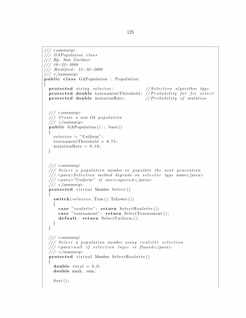
125
/// <summary>/// GAPopulation c l a s s/// By : Sam Gardner/// 10−22−2008/// Modi f i ed : 12−16−2008/// </summary>pub l i c c l a s s GAPopulation : Populat ion{
protected s t r i n g s e l e c t o r ; // S e l e c t i o n a l g o r i t hm typeprotected double tournamentThreshold ; // P r o b a b i l i t y f o r f i t s e l e c tprotected double mutationRate ; // P r o b a b i l i t y o f mutat ion
/// <summary>/// Create a new GA popu l a t i on/// </summary>pub l i c GAPopulation ( ) : base ( ){
s e l e c t o r = ”Uniform” ;tournamentThreshold = 0 . 7 5 ;mutationRate = 0 . 1 0 ;
}
/// <summary>/// S e l e c t a popu l a t i on member to popu l a t e t he nex t g ene ra t i on/// <para>S e l e c t i o n method depends on s e l e c t o r t ype name</para>/// <para>”Uniform” i f unrecognized </para>/// </summary>protected v i r t u a l Member S e l e c t ( ){
switch ( s e l e c t o r . Trim ( ) . ToLower ( ) ){
case ” r o u l e t t e ” : return Se l e c tRou l e t t e ( ) ;case ”tournament” : return SelectTournament ( ) ;de f au l t : return Se lectUni form ( ) ;
}}
/// <summary>/// S e l e c t a popu l a t i on member us ing r o u l e t t e s e l e c t i o n/// <para>n u l l i f s e l e c t i o n l o g i c i s f lawed </para>/// </summary>protected v i r t u a l Member Se l e c tRou l e t t e ( ){
double t o t a l = 0 . 0 ;double mark , sum ;
Sort ( ) ;

126
f o r each (Member m in member)t o t a l += m. F i tne s s ;
mark = rand . NextDouble ( t o t a l ) ;
sum = 0 . 0 ;f o r each (Member m in member){
sum += m. F i tne s s ;
i f (sum >= mark)return m;
}
return nu l l ;}
/// <summary>/// S e l e c t a popu l a t i on member us ing tournament s e l e c t i o n/// </summary>protected v i r t u a l Member SelectTournament ( ){
i n t one = rand . NextInt (member . Count ) ;i n t two = rand . NextInt (member . Count ) ;i f ( rand . Chance ( tournamentThreshold ) )
return (member [ one ] . F i tne s s > member [ two ] . F i tne s s )? member [ one ] : member [ two ] ;
return (member [ one ] . F i tne s s > member [ two ] . F i tne s s )? member [ two ] : member [ one ] ;
}
/// <summary>/// S e l e c t a popu l a t i on member us ing uniform s e l e c t i o n/// </summary>protected v i r t u a l Member Se lectUni form ( ){
i n t index = rand . NextInt (member . Count ) ;
return member [ index ] ;}
/// <summary>/// Replace the popu l a t i on wi th the nex t g ene ra t i on/// </summary>pub l i c ove r r i d e void Next ( ){
List<Member> next = new List<Member>() ;Member f , m, c ;
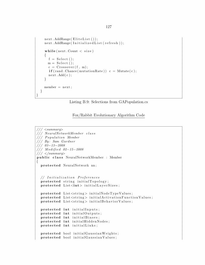
127
next . AddRange( E l i t e L i s t ( ) ) ;next . AddRange( I n i t i a l i z e d L i s t ( r e f r e s h ) ) ;
whi le ( next . Count < s i z e ){
f = S e l e c t ( ) ;m = Se l e c t ( ) ;c = Crossover ( f , m) ;i f ( rand . Chance ( mutationRate ) ) c = Mutate ( c ) ;next .Add( c ) ;
}
member = next ;}
}
Listing B.9: Selections from GAPopulation.cs
Fox/Rabbit Evolutionary Algorithm Code
/// <summary>/// NeuralNetworkMember c l a s s/// Popu la t ion Member/// By : Sam Gardner/// 03−13−2008/// Modi f i ed 02−15−2008/// </summary>pub l i c c l a s s NeuralNetworkMember : Member{
protected NeuralNetwork nn ;
// I n i t i a l i z a t i o n Pre f e r ence sprotected s t r i n g i n i t i a lTopo l o gy ;protected List<int> i n i t i a l L a y e r S i z e s ;
protected List<s t r i ng > in i t ia lNodeTypeValues ;protected List<s t r i ng > i n i t i a lAc t i v a t i onFunc t i onVa lu e s ;protected List<s t r i ng > i n i t i a lB ehav i o rVa l u e s ;
protected i n t i n i t i a l I n p u t s ;protected i n t i n i t i a lOu tpu t s ;protected i n t i n i t i a l B i a s e s ;protected i n t i n i t i a lH iddenNodes ;protected i n t i n i t i a l L i n k s ;
protected bool i n i t i a lGaus s i anWe ight s ;protected bool i n i t i a lGau s s i anVa lu e s ;
128
protected bool i n i t i a lGau s s i a nAc t i v a t i o nS l op e s ;protected bool i n i t i a lGau s s i anAc t i v a t i onL im i t s ;protected bool i n i t i a lGaus s i anQs ;protected bool i n i t i a lGau s s i anDt s ;protected bool i n i t i a lGaus s i anHL imi t s ;
protected double i n i t i a lWe i gh t ;protected double in i t ia lWeightRange ;protected double i n i t i a lV a l u e ;protected double i n i t i a lVa lueRange ;protected double i n i t i a lA c t i v a t i o n S l o p e ;protected double i n i t i a lAc t i v a t i onS l opeRange ;protected double i n i t i a lAc t i va t i onMax ;protected double in i t ia lAct ivat ionMaxRange ;protected double i n i t i a lAc t i v a t i onMin ;protected double i n i t i a lAct ivat i onMinRange ;
protected double i n i t i a lQ ;protected double in i t i a lQRange ;protected double i n i t i a l D t ;protected double i n i t i a lDtRange ;protected i n t i n i t i a lHL im i t ;protected i n t in i t i a lHLimitRange ;
// Mutation and Crossover Pre f e r ence sprotected List<s t r i ng > nodeTypeValues ;protected List<s t r i ng > act ivat ionFunct ionVa lues ;protected List<s t r i ng > behaviorValues ;
protected bool parametricMutation ;protected bool s t ruc tura lMutat ion ;protected bool temperatureBasedMutation ;
// Parametric Pre f e r ence sprotected bool weightMutation ;protected bool valueMutation ;protected bool actFuncMutation ;protected bool actSlopeMutat ion ;protected bool actLimitMutation ;protected bool actCenterLock ;protected bool actRangeLock ;protected bool qMutation ;protected bool dtMutation ;protected bool hLimitMutation ;protected bool behaviorMutation ;
protected double biasValue ;
protected double weightSca le ;
129
protected double va lueSca l e ;protected double actFuncChangeRate ;protected double ac tS l opeSca l e ;protected double ac tL imi tSca l e ;protected double qSca le ;protected double dtSca l e ;protected i n t hLimitSca le ;protected double behaviorChangeRate ;
// S t r u c t u r a l Pre f e r ence sprotected i n t maxNodeAdd ;protected i n t minNodeAdd ;protected i n t maxNodeDel ;protected i n t minNodeDel ;protected i n t maxNodeRetype ;protected i n t minNodeRetype ;
protected bool addLinksWithNodes ;
protected i n t maxLinkAdd ;protected i n t minLinkAdd ;protected i n t maxLinkDel ;protected i n t minLinkDel ;
protected double l inkIOBias ;
protected bool a l l owSe l fL i nk s ;protected bool a l l owDupl i ca teL inks ;protected bool a l lowMirrorL inks ;protected bool a l lowCrossL inks ;protected bool al lowBackLinks ;
/// <summary>/// Create a new neura l network member/// </summary>pub l i c NeuralNetworkMember ( ) : base ( ){
nn = new NeuralNetwork ( ) ;
i n i t i a l L a y e r S i z e s = new List<int >() ;
in i t ia lNodeTypeValues = new List<s t r i ng >() ;i n i t i a lAc t i v a t i onFunc t i onVa lu e s = new List<s t r i ng >() ;i n i t i a lB ehav i o rVa l u e s = new List<s t r i ng >() ;
nodeTypeValues = new List<s t r i ng >() ;ac t ivat i onFunct ionVa lues = new List<s t r i ng >() ;behaviorValues = new List<s t r i ng >() ;
130
// I n i t i a l i z a t i o n Pre f e r ence si n i t i a lTopo l o gy = ”FF” ;i n i t i a l L a y e r S i z e s .Add ( 1 0 ) ;
in i t ia lNodeTypeValues . AddRange( NodeTypeValueList ) ;i n i t i a lAc t i v a t i onFunc t i onVa lu e s .Add( ”Tanh” ) ;i n i t i a lB ehav i o rVa l u e s .Add( ”Ratio ” ) ;
i n i t i a l I n p u t s = 2 ;i n i t i a lOu tpu t s = 2 ;i n i t i a l B i a s e s = 1 ;in i t i a lH iddenNodes = 10 ;i n i t i a l L i n k s = 42 ;
i n i t i a lGaus s i anWe ight s = f a l s e ;i n i t i a lGau s s i anVa lu e s = f a l s e ;i n i t i a lGau s s i a nAc t i v a t i o nS l op e s = f a l s e ;i n i t i a lGau s s i anAc t i v a t i onL im i t s = f a l s e ;i n i t i a lGaus s i anQs = f a l s e ;i n i t i a lGau s s i anDt s = f a l s e ;i n i t i a lGaus s i anHL imi t s = f a l s e ;
i n i t i a lWe i gh t = 0 . 0 ;in i t ia lWeightRange = 0 . 5 ;i n i t i a lV a l u e = 0 . 0 ;i n i t i a lVa lueRange = 3 . 0 ;i n i t i a lA c t i v a t i o n S l o p e = 1 . 0 ;i n i t i a lAc t i v a t i onS l opeRange = 0 . 0 ;i n i t i a lAc t i va t i onMax = 1 . 0 ;in i t ia lAct ivat ionMaxRange = 0 . 0 ;i n i t i a lAc t i v a t i onMin = −1.0;in i t i a lAct ivat i onMinRange = 0 . 0 ;
i n i t i a lQ = 0 . 0 ;in i t i a lQRange = 1 . 0 ;i n i t i a l D t = 1 . 0 ;in i t i a lDtRange = 0 . 0 ;i n i t i a lHL im i t = 0 ;in i t ia lHLimitRange = 0 ;
// Mutation and Crossover Pre f e r ence snodeTypeValues . AddRange( in i t ia lNodeTypeValues ) ;ac t ivat i onFunct ionVa lues . AddRange( i n i t i a lAc t i v a t i onFunc t i onVa lu e s ) ;behaviorValues . AddRange( i n i t i a lB ehav i o rVa l u e s ) ;
parametricMutation = true ;s t ruc tura lMutat ion = true ;temperatureBasedMutation = true ;
// Parametric Pre f e r ence s
131
weightMutation = true ;valueMutation = true ;actFuncMutation = f a l s e ;actSlopeMutat ion = f a l s e ;actLimitMutation = f a l s e ;actCenterLock = f a l s e ;actRangeLock = f a l s e ;qMutation = true ;dtMutation = f a l s e ;hLimitMutation = f a l s e ;behaviorMutation = f a l s e ;
b iasValue = 1 . 0 ;
we ightSca l e = 1 . 0 ;va lueSca l e = 10 . 0 ;actFuncChangeRate = 0 . 0 0 1 ;a c tS l opeSca l e = 0 . 1 ;a c tL imi tSca l e = 0 . 1 ;qSca le = 0 . 1 ;d tSca l e = 0 . 1 ;hLimitSca le = 10 ;behaviorChangeRate = 0 . 0 0 1 ;
// S t r u c t u r a l Pre f e r ence smaxNodeAdd = 3 ;minNodeAdd = 1 ;maxNodeDel = 3 ;minNodeDel = 1 ;maxNodeRetype = 3 ;minNodeRetype = 1 ;
addLinksWithNodes = f a l s e ;
maxLinkAdd = 20 ;minLinkAdd = 4 ;maxLinkDel = 5 ;minLinkDel = 1 ;
l inkIOBias = 0 . 2 ;
a l l owSe l fL i nk s = f a l s e ;a l l owDupl i ca teL inks = f a l s e ;a l l owMirrorL inks = f a l s e ;a l l owCrossL inks = f a l s e ;a l lowBackLinks = f a l s e ;
}
/// <summary>/// I n i t i a l i z e t h i s neura l network member
132
/// </summary>pub l i c ove r r i d e Member I n i t i a l i z e ( ){
nn . Clear ( ) ;
switch ( i n i t i a lTopo l o gy . ToLower ( ) ){
case ” f f ” : In i t i a l i z eFeedForward ( ) ; break ;case ”cc− f f ” : In i t ia l i zeCrossConnectedFeedForward ( ) ; break ;case ” r e cu r r en t ” : I n i t i a l i z eR e c u r r e n t ( ) ; break ;case ” fc− f f ” : In i t ia l i z eFu l lyConnectedFeedForward ( ) ; break ;case ” f c ” : I n i t i a l i z eFu l l yConne c t ed ( ) ; break ;de f au l t : /∗ random ∗/ In i t i a l i z eRandom ( ) ; break ;
}
i f ( ! double . IsNaN( biasValue ) ) SetAl lB iasVa lues ( biasValue ) ;
return t h i s ;}
protected void In i t i a l i z eRandom ( ){
Neuron node ;L i s t<int> from , to ;i n t f , t ;bool va l i d ;
f o r ( i n t b = 0 ; b < i n i t i a l B i a s e s ; b++){
node = InitialRandomNode ( ) ;nn .Add( node ) ;
}
f o r ( i n t i = 0 ; i < i n i t i a l I n p u t s ; i++){
node = InitialRandomNode ( ) ;nn . AddInput ( node ) ;
}
f o r ( i n t h = 0 ; h < i n i t i a lH iddenNodes ; h++){
node = InitialRandomNode ( ) ;nn .Add( node ) ;
}
f o r ( i n t o = 0 ; o < i n i t i a lOu tpu t s ; o++){
node = InitialRandomNode ( ) ;nn . AddOutput ( node ) ;
}

133
// Linksf o r ( i n t l = 0 ; l < i n i t i a l L i n k s ; l++){
from = rand . Chance ( l inkIOBias )? nn . InputNodeIndices ( ) : nn . NonIONodeIndices ( ) ;
to = rand . Chance ( l inkIOBias )? nn . OutputNodeIndices ( ) : nn . NonIONodeIndices ( ) ;
i f ( from . Count > 0 && to . Count > 0){
from = RandomGenerator . Shu f f l e ( from ) ;to = RandomGenerator . Shu f f l e ( to ) ;
v a l i d = f a l s e ;f = 0 ;t = −1;whi le ( ! v a l i d ){
t++; i f ( t >= to . Count ) { t = 0 ; f++; }i f ( f >= from . Count ) break ;
v a l i d = LinkIsVa l id ( from [ f ] , to [ t ] ) ;}
i f ( v a l i d )nn . Connect ( from [ f ] , to [ t ] ,
Init ialRandomValue ( in i t i a lGauss i anWeight s ,i n i t i a lWe igh t ,in i t ia lWeightRange ) ) ;
}}
}
/// <summary>/// Return a mutated copy o f t h i s neura l network member/// </summary>pub l i c ove r r i d e Member Mutate ( ){
NeuralNetworkMember m = t h i s . Copy ( ) as NeuralNetworkMember ;double temp = temperatureBasedMutation
? m. InstantaneousTemperature : 1 . 0 ;
i f (m. parametricMutation ) m. MutateParametric ( temp ) ;i f (m. s t ruc tura lMutat ion ) m. MutateStructura l ( temp ) ;
i f ( ! double . IsNaN( biasValue ) ) m. SetAl lB iasValues ( biasValue ) ;
return m;}
/// <summary>

134
/// Parametric mutat ion/// </summary>/// <param name=”temp”> i n s t an t aneou s tempera ture o f member</param>protected void MutateParametric ( double temp){
i f ( weightMutation ) MutateWeights ( temp ) ;i f ( valueMutation ) MutateValues ( temp ) ;i f ( actFuncMutation ) MutateAct ivat ionFunct ions ( temp ) ;i f ( actSlopeMutat ion ) MutateAct ivat ionSlopes ( temp ) ;i f ( actLimitMutation ) MutateAct ivat ionLimits ( temp ) ;
i f ( qMutation ) MutateQValues ( temp ) ;i f ( dtMutation ) MutateDtValues ( temp ) ;i f ( hLimitMutation ) MutateHistoryLimits ( temp ) ;i f ( behaviorMutation ) MutateBehaviors ( temp ) ;
}
protected void MutateWeights ( double temp){
double value ;
f o r ( i n t l = 0 ; l < nn . LinkCount ; l++){
value = nn . Weight ( l ) ;va lue += GNARLPreturbation ( weightScale , temp ) ;nn . SetWeight ( l , va lue ) ;
}}
/// <summary>/// Return t rue i f l i n k between s p e c i f i e d i n d i c e s would be v a l i d/// accord ing to cur r en t s e t t i n g s/// </summary>/// <param name=”from”>source node index </param>/// <param name=”to”>d e s t i n a t i o n node index </param>protected bool L inkI sVa l id ( i n t from , i n t to ){
i f ( ! a l l owSe l fL i nk s && from == to ) return f a l s e ;i f ( ! a l l owDupl i ca teL inks && nn . ConnectedTo ( from , to ) ) return f a l s e ;i f ( ! a l l owMirrorL inks && nn . ConnectedTo ( to , from ) ) return f a l s e ;i f ( ! a l lowCrossL inks && nn . I sCrossL ink ( from , to ) ) return f a l s e ;i f ( ! al lowBackLinks && nn . IsBackLink ( from , to ) ) return f a l s e ;
return true ;}
/// <summary>/// S t r u c t u r a l mutat ion/// </summary>/// <param name=”temp”> i n s t an t aneou s tempera ture o f member</param>protected void MutateStructura l ( double temp)

135
{MutateNodeAdd( temp ) ;MutateNodeDel ( temp ) ;MutateNodeRetype ( temp ) ;
MutateLinkAdd ( temp ) ;MutateLinkDel ( temp ) ;
}
protected void MutateNodeDel ( double temp){
i n t num = GNARLModifications (minNodeDel , maxNodeDel , temp ) ;L i s t<int> i n d i c e s ;
f o r ( i n t i = 0 ; i < num; i++){
i n d i c e s = nn . NonIONodeIndices ( ) ;i f ( i n d i c e s . Count > 0)
nn . RemoveAt( i n d i c e s [ rand . NextInt ( i n d i c e s . Count ) ] ) ;}
}
/// <summary>/// Return a copy o f t h i s neura l network member c ro s s ed wi th another/// </summary>/// <param name=”o the r”> f a t h e r member</param>pub l i c ove r r i d e Member Crossover (Member other ){
NeuralNetworkMember c = t h i s . ShallowCopy ( ) as NeuralNetworkMember ;i f ( other i s NeuralNetworkMember ){
NeuralNetworkMember f a th e r = other as NeuralNetworkMember ;NeuralNetworkMember mother = t h i s ;L i s t<int> ChildToMother = new List<int >() ;L i s t<int> ChildToFather = new List<int >() ;L i s t<int> MotherToChild = new List<int >() ;L i s t<int> FatherToChild = new List<int >() ;
L i s t<int> mHidden , fHidden , cHidden ;bool inheritFromMother ;i n t nodes , l i n k s ;i n t mlink , f l i n k ;i n t mi , f i ;i n t mdst , f d s t ;i n t i ;
// Inpu t snodes = Math .Max( mother . nn . InputCount , f a t h e r . nn . InputCount ) ;f o r ( i = 0 ; i < nodes ; i++)
i f ( rand . Chance ( 0 . 5 ) )
136
{i f ( i < mother . nn . InputCount )
c . nn . AddInput ( mother . nn . InputNode ( i ) . Copy ( ) ) ;}e l s e{
i f ( i < f a t h e r . nn . InputCount )c . nn . AddInput ( f a th e r . nn . InputNode ( i ) . Copy ( ) ) ;
}
// Outputsnodes = Math .Max( mother . nn . OutputCount , f a t h e r . nn . OutputCount ) ;f o r ( i = 0 ; i < nodes ; i++)
i f ( rand . Chance ( 0 . 5 ) ){
i f ( i < mother . nn . OutputCount )c . nn . AddOutput ( mother . nn . OutputNode ( i ) . Copy ( ) ) ;
}e l s e{
i f ( i < f a t h e r . nn . OutputCount )c . nn . AddOutput ( f a t h e r . nn . OutputNode ( i ) . Copy ( ) ) ;
}
// Non−IO NodesmHidden = mother . nn . NonIONodeIndices ( ) ;fHidden = fa th e r . nn . NonIONodeIndices ( ) ;nodes = Math .Max(mHidden . Count , fHidden . Count ) ;f o r ( i = 0 ; i < nodes ; i++)
i f ( rand . Chance ( 0 . 5 ) ){
i f ( i < mHidden . Count )c . nn .Add( mother . nn . Node (mHidden [ i ] ) . Copy ( ) ) ;
}e l s e{
i f ( i < fHidden . Count )c . nn .Add( f a th e r . nn . Node ( fHidden [ i ] ) . Copy ( ) ) ;
}
// Bui ld index mapsf o r ( i = 0 ; i < c . nn . InputCount ; i++){
ChildToMother .Add( ( i < mother . nn . InputCount )? mother . nn . IndexOf ( mother . nn . InputNode ( i ) ) : −1);
ChildToFather .Add( ( i < f a t h e r . nn . InputCount )? f a th e r . nn . IndexOf ( f a th e r . nn . InputNode ( i ) ) : −1);
}
f o r ( i = 0 ; i < c . nn . OutputCount ; i++)

137
{ChildToMother .Add( ( i < mother . nn . OutputCount )
? mother . nn . IndexOf ( mother . nn . OutputNode ( i ) ) : −1);ChildToFather .Add( ( i < f a t h e r . nn . OutputCount )
? f a th e r . nn . IndexOf ( f a th e r . nn . OutputNode ( i ) ) : −1);}
cHidden = c . nn . NonIONodeIndices ( ) ;f o r ( i = 0 ; i < cHidden . Count ; i++){
ChildToMother .Add( ( i < mHidden . Count ) ? mHidden [ i ] : −1);ChildToFather .Add( ( i < fHidden . Count ) ? fHidden [ i ] : −1);
}
f o r ( i = 0 ; i < mother . nn . NodeCount ; i++)MotherToChild .Add( ChildToMother . IndexOf ( i ) ) ;
f o r ( i = 0 ; i < f a t h e r . nn . NodeCount ; i++)FatherToChild .Add( ChildToFather . IndexOf ( i ) ) ;
// Linksf o r ( i n t n = 0 ; n < c . nn . NodeCount ; n++){
mi = ChildToMother [ n ] ;f i = ChildToFather [ n ] ;mlink = (mi != −1) ? mother . nn . Node (mi ) . OutputCount : 0 ;f l i n k = ( f i != −1) ? f a th e r . nn . Node ( f i ) . OutputCount : 0 ;l i n k s = Math .Max( mlink , f l i n k ) ;f o r ( i = 0 ; i < l i n k s ; i++){
mdst = ( i < mlink )? MotherToChild [ mother . nn . IndexOf (
mother . nn . Node (mi ) . Output ( i ) ) ]: i n t . MinValue ;
f d s t = ( i < f l i n k )? FatherToChild [ f a t h e r . nn . IndexOf (
f a th e r . nn . Node ( f i ) . Output ( i ) ) ]: i n t . MinValue ;
inheritFromMother = f a l s e ;i f ( rand . Chance ( 0 . 5 ) ) inheritFromMother = true ;i f (mdst == −1) inheritFromMother = f a l s e ;i f ( f d s t == −1) inheritFromMother = true ;
i f ( inheritFromMother ){
i f ( i < mlink )c . nn . Connect (n , mdst , mother . nn . Node (mi ) . OutputWeight ( i ) ) ;
}e l s e
138
{i f ( i < f l i n k )
c . nn . Connect (n , fds t , f a t h e r . nn . Node ( f i ) . OutputWeight ( i ) ) ;}
}}
}
i f ( ! double . IsNaN( biasValue ) ) c . SetAl lB iasValues ( biasValue ) ;
return c ;}
}
Listing B.10: Selections from NeuralNetworkMember.cs
/// <summary>/// FoxRabbitEA c l a s s/// Evo lu t i onary Algor i thm/// By : Sam Gardner/// 05−23−2008/// Modi f i ed : 12−04−2008/// </summary>pub l i c c l a s s FoxRabbitEA : Evolut ionaryAlgor ithm{
protected Simulat ion sim ;
protected i n t t r i a l s ;
protected bool saveEveryReplay ;protected bool saveGenerat iona lBestReplays ;protected bool saveBestReplays ;
/// <summary>/// Create a new fox r a b b i t EA/// </summary>pub l i c FoxRabbitEA ( ) : base ( ){
sim = new Simulat ion ( ) ;
t r i a l s = 30 ;
saveEveryReplay = f a l s e ;saveGenerat iona lBestReplays = f a l s e ;saveBestReplays = true ;
}
/// <summary>
139
/// Return a new popu l a t i on s u i t a b l e f o r use wi th the ea/// </summary>/// <param name=”type”>popu l a t i on type name</param>/// <param name=”useId”>popu l a t i on use t ype name</param>pub l i c ove r r i d e Populat ion NewPopulation ( s t r i n g type , s t r i n g use ){
i n t index = populat ion . Count ;Populat ion pop = MakePopulation ( type ) ;NeuralNetworkMember prototype = new NeuralNetworkMember ( ) ;prototype . MaxPoss ib leFitness = maxPoss ib leF i tness ;
prototype . I n i t i a l B i a s e s = 1 ;prototype . I n i t i a l I n p u t s = 24 ;prototype . I n i t i a lOu tpu t s = 2 ;prototype . I n i t i a lAc t i va t i onFunc t i onVa lu e s . Clear ( ) ;prototype . I n i t i a lAc t i va t i onFunc t i onVa lu e s .Add( ”Tanh” ) ;prototype . I n i t i a lGau s s i anAc t i v a t i onS l op e s = f a l s e ;prototype . I n i t i a lA c t i v a t i o nS l o p e = 1 ;prototype . I n i t i a lAc t i va t i onS l opeRange = 0 ;prototype . I n i t i a lGau s s i anAc t i v a t i onL im i t s = f a l s e ;prototype . In i t ia lAct ivat ionMaxRange = 0 ;prototype . In i t i a lAct ivat ionMinRange = 0 ;
prototype . I n i t i a lBehav i o rVa lu e s . Clear ( ) ;prototype . I n i t i a lBehav i o rVa lu e s .Add( ”Ratio ” ) ;
prototype . Act ivat ionFunct ionValues . Clear ( ) ;prototype . Act ivat ionFunct ionValues . AddRange(
prototype . I n i t i a lAc t i va t i onFunc t i onVa lu e s ) ;
prototype . BehaviorValues . Clear ( ) ;prototype . BehaviorValues . AddRange( prototype . I n i t i a lBehav i o rVa lu e s ) ;
prototype . Structura lMutat ion = f a l s e ;prototype . AllowBackLinks = true ;prototype . Al lowDupl icateLinks = f a l s e ;prototype . Al lowCrossLinks = true ;prototype . Al lowMirrorLinks = true ;prototype . A l lowSe l fL inks = true ;
pop . Prototype = prototype ;pop .Name = s t r i n g . Format ( ”Fox {0}” , index ) ;pop . Use = ” Defau l t ” ;pop . S i z e = 64 ;pop . E l i t e = 3 ;
i f ( pop i s GNARLPopulation ){
( pop as GNARLPopulation ) . Surv iva lRate = 0 . 5 ;}

140
i f ( pop i s GAPopulation ){
( pop as GAPopulation ) . MutationRate = 0 . 0 1 ;( pop as GAPopulation ) . S e l e c t o r = ” Roulette ” ;( pop as GAPopulation ) . TournamentThreshold = 0 . 7 5 ;
}
return pop ;}
/// <summary>/// I n i t i a l i z e t he f o x r a b b i t ea/// </summary>pub l i c ove r r i d e void I n i t i a l i z e ( ){
base . I n i t i a l i z e ( ) ;sim . Reset ( ) ;
}
/// <summary>/// Eva lua te a popu l a t i on member/// </summary>/// <param name=”popIndex”>popu l a t i on index </param>/// <param name=”memberIndex”>member index </param>/// <re turns > f i t n e s s va lue </re turns >pub l i c ove r r i d e double EvaluateMember (Member ind iv idua l ,
i n t popIndex ,i n t memberIndex )
{i f ( i nd i v i dua l i s NeuralNetworkMember ){
NeuralNetworkMember m = ind i v i dua l as NeuralNetworkMember ;double f i t n e s s = 0 . 0 ;
sim .FoxNN = m.NN. Copy ( ) ;
f o r ( i n t t = 0 ; t < t r i a l s ; t++){
sim . Reset ( ) ;sim .Run ( ) ;i f ( l og != nu l l ){
sim . Replay . Generation = genera t i on ;sim . Replay . Populat ion = populat ion [ popIndex ] . Name ;sim . Replay . MemberIndex = memberIndex ;sim . Replay . Tr i a l = t ;
( s t a t e as FoxRabbitState ) . Upda t eTr i a lL ev e l S t a t i s t i c s (popIndex , memberIndex , sim . Replay ) ;
141
i f ( saveEveryReplay )sim . Replay . Save (
s t r i n g . Format ( ”Replay−{0}−G{1}−{2}−M{3}−T{4} . r ep lay ” ,name ,generat ion ,populat ion [ popIndex ] . Name,memberIndex ,t ) ) ;
i f ( saveGenerat iona lBestReplays )i f ( ( s t a t e as FoxRabbitState ) . I sGenerat iona lBestRep lay (
popIndex , sim . Replay ) )sim . Replay . Save (
s t r i n g . Format ( ”BestReplay−{0}−{1}−G{2} . r ep lay ” ,name ,populat ion [ popIndex ] . Name,gene ra t i on ) ) ;
i f ( saveBestReplays )i f ( ( l og as FoxRabbitLog ) . IsBestReplay (
popIndex , sim . Replay ) )sim . Replay . Save (
s t r i n g . Format ( ”BestReplay−{0}−{1}. r ep lay ” ,name ,populat ion [ popIndex ] . Name ) ) ;
}f i t n e s s += sim . Score ( ) ;
}f i t n e s s /= ( double ) t r i a l s ;
return f i t n e s s ;}
return 0 . 0 ;}
}
Listing B.11: Selections from FoxRabbitEA.cs

142
Fox/Rabbit Simulation Code
/// <summary>/// En t i t y c l a s s/// By : Sam Gardner/// 05−25−2008/// Modi f i ed : 12−16−2008/// </summary>pub l i c ab s t r a c t c l a s s Entity{
protected RandomGenerator rand ;
protected List<s t r i ng > comment ;
protected double rad iu s ; // A l l e n t i t i e s are c i r c u l a rprotected Vector2 po s i t i o n ;protected Vector2 v e l o c i t y ;protected Vector2 a c c e l e r a t i o n ;
protected double t r a n s l a t i o nS c a l a r ;protected Vector2 t r a n s l a t i o n ;protected bool s o l i d C o l l i s i o n ;
protected Sc r i p t s c r i p t ;
protected bool startAnywhere ;protected Vector2 s t a r t ;protected Vector2 startRange ;protected double s t a r tD i s t anc e ;protected double startAzimuth ;protected double startAzimuthRange ;
protected double maxSpeed ;protected double maxAccel ;protected double veloc i tyDecayRate ;
/// <summary>/// Base c on s t r u c t o r/// </summary>pub l i c Entity ( ){
rand = new RandomGenerator ( ) ;
comment = new List<s t r i ng >() ;
r ad iu s = 0 . 5 ;p o s i t i o n = new Vector2 ( 0 . 0 , 0 . 0 ) ;v e l o c i t y = new Vector2 ( 0 . 0 , 0 . 0 ) ;
143
a c c e l e r a t i o n = new Vector2 ( 0 . 0 , 0 . 0 ) ;
t r a n s l a t i o nS c a l a r = 1 . 0 ;t r a n s l a t i o n = new Vector2 ( 0 . 0 , 0 . 0 ) ;s o l i d C o l l i s i o n = f a l s e ;
s c r i p t = nu l l ;
startAnywhere = true ;s t a r t = new Vector2 ( 0 . 0 , 0 . 0 ) ;startRange = new Vector2 ( 0 . 0 , 0 . 0 ) ;s t a r tD i s t anc e = 0 . 0 ;startAzimuth = 0 . 0 ;startAzimuthRange = 180 . 0 ;
maxSpeed = 8 . 0 ;maxAccel = 1 . 0 ;ve loc i tyDecayRate = 0 . 1 ;
}
/// <summary>/// Return a s t a r t i n g p o s i t i o n t h a t meets s t a r t p r e f e r e n c e s/// </summary>pub l i c Vector2 S t a r tPo s i t i on ( ){
Vector2 s = new Vector2 ( ) ;
i f ( S t a r tRe l a t i v e ){
double azimuth = startAzimuth ;i f ( startAzimuthRange > 0 . 0 )
azimuth += rand . NextCenteredDouble ( 0 . 0 , startAzimuthRange ) ;azimuth = Angle .Rad( Angle . Azimuth2Deg ( azimuth ) ) ;
s .X = s t a r t .X + ( ( s t a r tD i s t anc e + rad iu s ) ∗ Math . Cos ( azimuth ) ) ;s .Y = s t a r t .Y + ( ( s t a r tD i s t anc e + rad iu s ) ∗ Math . Sin ( azimuth ) ) ;
}e l s e{
s .X = s t a r t .X;s .Y = s t a r t .Y;i f ( startRange .X > 0 . 0 )
s .X += rand . NextCenteredDouble ( 0 . 0 , startRange .X) ;i f ( startRange .Y > 0 . 0 )
s .Y += rand . NextCenteredDouble ( 0 . 0 , startRange .Y) ;}
return s ;}
/// <summary>
144
/// Compute nex t a c t i on/// <para>u s u a l l y t he nex t a c c e l e r a t i o n vec tor </para>/// </summary>/// <param name=”sim”> s imu l a t i on to compute for </param>pub l i c v i r t u a l void ComputeNextAction ( S imulat ion sim ){
i f ( s c r i p t != nu l l )a c c e l e r a t i o n = s c r i p t . Next ( ) ;
e l s eCompute ( sim ) ;
EnforceLimits ( ) ;}
/// <summary>/// Perform any computat ions and ad jus tment s nece s sa ry f o r movement/// </summary>/// <param name=”sim”> s imu l a t i on to compute for </param>protected v i r t u a l void Compute ( S imulat ion sim ){
a c c e l e r a t i o n . Zero ( ) ;}
/// <summary>/// Adjus t a c c e l e r a t i o n and v e l o c i t y to s a t i s f y l i m i t s/// </summary>protected v i r t u a l void EnforceLimits ( ){
// Enforce maximum a c c e l e r a t i o ni f ( a c c e l e r a t i o n . Length ( ) > maxAccel )
a c c e l e r a t i o n = a c c e l e r a t i o n . Unit ( ) ∗ maxAccel ;
v e l o c i t y += ac c e l e r a t i o n ;
// Enforce maximum v e l o c i t yi f ( v e l o c i t y . Length ( ) > maxSpeed )
v e l o c i t y = v e l o c i t y . Unit ( ) ∗ maxSpeed ;
t r a n s l a t i o nS c a l a r = 1 . 0 ;}
/// <summary>/// Return a v e c t o r from t h i s e n t i t y ’ s c en t e r to t h a t o f another/// </summary>pub l i c Vector2 CenterSeparat ion ( Entity other ){
return other . p o s i t i o n − po s i t i o n ;}
/// <summary>/// Return a v e c t o r from the edge o f t h i s e n t i t y

145
/// to the edge o f another/// <para>t a k e s r a d i i i n t o account </para>/// </summary>pub l i c Vector2 Separat ion ( Entity other ){
Vector2 cs = CenterSeparat ion ( other ) ;return cs − ( cs . Unit ( ) ∗ ( rad iu s + other . r ad iu s ) ) ;
}
/// <summary>/// Return f r a c t i o n o f t r a n s l a t i o n b e f o r e/// t h i s e n t i t y c o l l i d e s w i th another/// <para >1.0 i n d i c a t e s no c o l l i s i o n </para>/// <para>/// Uses s i n g l e frame o f r e f e r e n c e t e chn i qu e/// Descr i bed by : Joe van den Heuvel and Mi les Jackson/// For : Gamasutra/// January 18 , 2002/// </para>/// </summary>pub l i c double Co l l i s i o n ( Entity other ){
double t = 1 . 0 ;
// Compute r e l a t i v e v e l o c i t y us ing the frame o f r e f e r en c e// where o t he r i s s t a t i o n a r yVector2 rv = v e l o c i t y − other . v e l o c i t y ;double rvmag = rv . Length ( ) ;
Vector2 rp = po s i t i o n .To( other . p o s i t i o n ) ;double r a d i i = rad iu s + other . r ad iu s ;
double rp do t rv = rp . Dot ( rv ) ;i f ( rp do t rv > 0 . 0 ) // Shor t c i r c u i t f o r wrong d i r e c t i o n
i f ( rvmag >= rp . Length ( ) − r a d i i ) // sc f o r not enough d i s t an c e{
// l e n g t h o f rp p r o j e c t e d onto rvdouble p = rp dot rv / rvmag ;// square o f c l o s e s t d i s t a n c e e n t i t i e s g e t to each o the rdouble d = rp . LengthSq ( ) − (p ∗ p ) ;i f (d <= r a d i i ∗ r a d i i ) // sc f o r doesn ’ t pass c l o s e enough{
double t r a v e l = p − Math . Sqrt ( r a d i i ∗ r a d i i − d ) ;i f ( t r a v e l <= rvmag ) // sc f o r doesn ’ t g e t t h e r e
t = t r a v e l / rvmag ;}
}
return t ;}
146
/// <summary>/// Return f r a c t i o n o f t r a n s l a t i o n b e f o r e t h i s e n t i t y/// c o l l i d e s w i th a wa l l/// <para >1.0 i n d i c a t e s no c o l l i s i o n </para>/// </summary>/// <param name=”sim”> s imu l a t i on to c o l l i d e in</param>pub l i c double Co l l i s i onWa l l s ( S imulat ion sim ){
double c o l l i s i o n = 1 . 0 ;
i f ( sim . F i e ld . Walls ){
double xWall = sim . F i e ld . Width / 2 .0 − rad iu s ;double yWall = sim . F i e ld . Height / 2 .0 − rad iu s ;double t ;
i f ( v e l o c i t y .X < 0 . 0 ){
t = (−xWall − po s i t i o n .X) / v e l o c i t y .X; // west wa l li f ( t >= 0.0 && t < 1 . 0 ) c o l l i s i o n = Math . Min( c o l l i s i o n , t ) ;
}e l s e i f ( v e l o c i t y .X > 0 . 0 ){
t = ( xWall − po s i t i o n .X) / v e l o c i t y .X; // ea s t wa l li f ( t >= 0.0 && t < 1 . 0 ) c o l l i s i o n = Math . Min( c o l l i s i o n , t ) ;
}
i f ( v e l o c i t y .Y < 0 . 0 ){
t = (−yWall − po s i t i o n .Y) / v e l o c i t y .Y; // nor th wa l li f ( t >= 0.0 && t < 1 . 0 ) c o l l i s i o n = Math . Min( c o l l i s i o n , t ) ;
}e l s e i f ( v e l o c i t y .Y > 0 . 0 ){
t = ( yWall − po s i t i o n .Y) / v e l o c i t y .Y; // sou th wa l li f ( t >= 0.0 && t < 1 . 0 ) c o l l i s i o n = Math . Min( c o l l i s i o n , t ) ;
}}
return c o l l i s i o n ;}
/// <summary>/// Check f o r en t i t y−to−e n t i t y c o l l i s i o n and s e t t r a n s l a t i o n s c a l a r/// </summary>/// <param name=”o the r”> e n t i t y to check c o l l i s i o n with </param>pub l i c void Co l l i d e ( Entity other ){
double t = Co l l i s i o n ( other ) ;t r a n s l a t i o nS c a l a r = Math . Min( t r an s l a t i o nS c a l a r , t ) ;i f ( t < 1 .0 && ! ( t h i s i s C r i t t e r && other i s C r i t t e r ) )
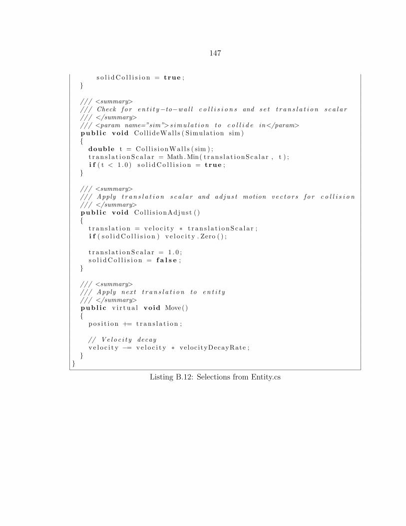
147
s o l i d C o l l i s i o n = true ;}
/// <summary>/// Check f o r en t i t y−to−wa l l c o l l i s i o n s and s e t t r a n s l a t i o n s c a l a r/// </summary>/// <param name=”sim”> s imu l a t i on to c o l l i d e in</param>pub l i c void Col l ideWal l s ( S imulat ion sim ){
double t = Co l l i s i onWa l l s ( sim ) ;t r a n s l a t i o nS c a l a r = Math . Min( t r an s l a t i o nS c a l a r , t ) ;i f ( t < 1 . 0 ) s o l i d C o l l i s i o n = true ;
}
/// <summary>/// Apply t r a n s l a t i o n s c a l a r and ad j u s t motion v e c t o r s f o r c o l l i s i o n/// </summary>pub l i c void Co l l i s i onAd ju s t ( ){
t r a n s l a t i o n = v e l o c i t y ∗ t r a n s l a t i o nS c a l a r ;i f ( s o l i d C o l l i s i o n ) v e l o c i t y . Zero ( ) ;
t r a n s l a t i o nS c a l a r = 1 . 0 ;s o l i d C o l l i s i o n = f a l s e ;
}
/// <summary>/// Apply nex t t r a n s l a t i o n to e n t i t y/// </summary>pub l i c v i r t u a l void Move ( ){
po s i t i o n += t r an s l a t i o n ;
// Ve l o c i t y decayv e l o c i t y −= ve l o c i t y ∗ veloc i tyDecayRate ;
}}
Listing B.12: Selections from Entity.cs

148
/// <summary>/// C r i t t e r e n t i t y/// By : Sam Gardner/// 05−23−2008/// Modi f i ed : 12−16−2008/// </summary>pub l i c c l a s s Cr i t t e r : Ent ity{
pub l i c c l a s s Cr i t t e rS en so r{
pub l i c double value ;pub l i c double i n t e n s i t y ;
}
protected s t r i n g r o l e ;
protected i n t sensorCount ;protected i n t s en so rReso lu t i on ;
protected List<Cr i t t e rSensor > s enso r ;protected List<Cr i t t e rSensor > s en s o rCe l l ;
/// <summary>/// Create a new c r i t t e r/// </summary>pub l i c Cr i t t e r ( ) : base ( ){
rand = new RandomGenerator ( ) ;
s enso r = new List<Cr i t t e rSensor >() ;s e n s o rCe l l = new List<Cr i t t e rSensor >() ;
r o l e = ” Cr i t t e r ” ;
sensorCount = 12 ;s en so rReso lu t i on = 30 ;
}
/// <summary>/// Return sensed i n t e n s i t y o f e n t i t y a t s p e c i f i e d d i s t a n c e/// <para > [0 .0 , 1.0] </ para>/// </summary>/// <param name=”d i s t an c e”>d i s t ance </param>/// <param name=”sim”> s imu l a t i on to sense </param>protected double I n t e n s i t y ( double di s tance , S imulat ion sim ){
double max = sim . F i e ld . MaxSeparationDistance ;i f ( d i s t anc e <= 0 . 0 )
return 1 . 0 ;
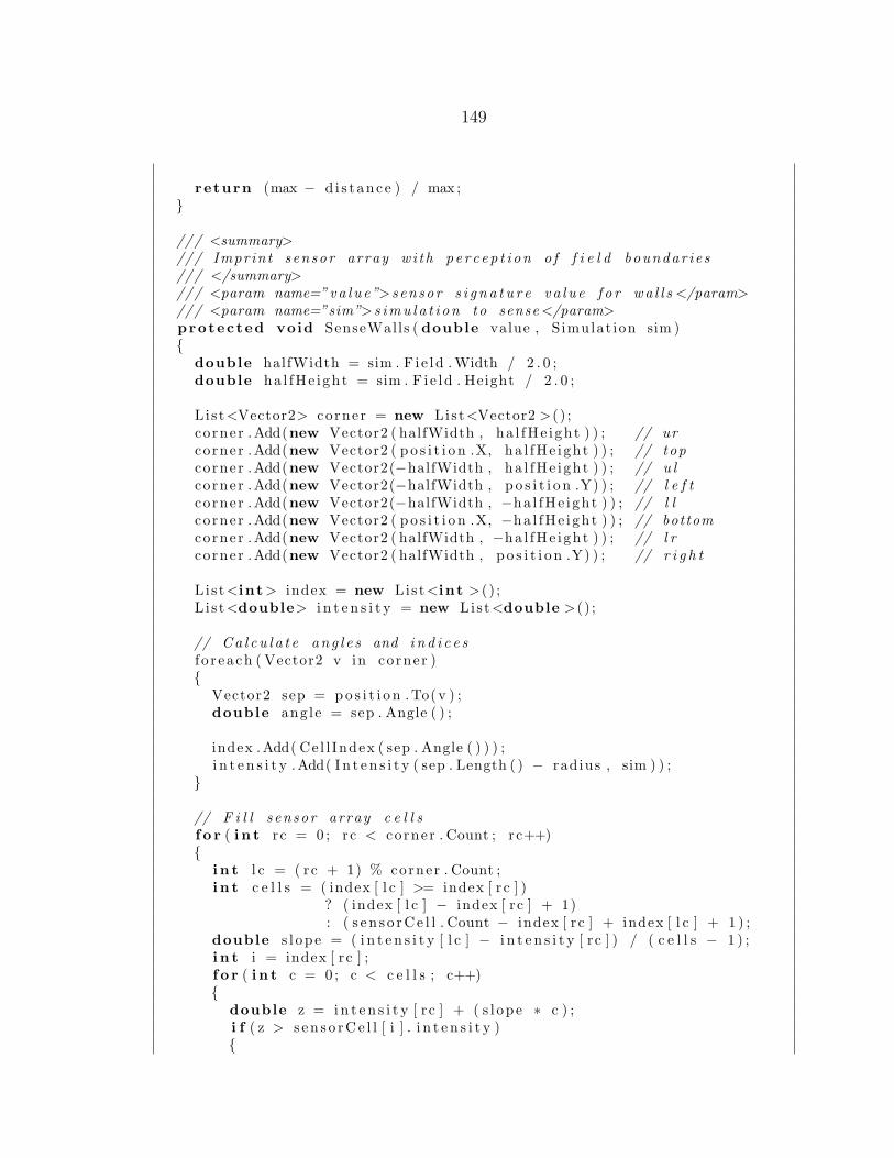
149
return (max − d i s t anc e ) / max ;}
/// <summary>/// Imprint sensor array wi th p e r c ep t i on o f f i e l d boundar i e s/// </summary>/// <param name=”va l u e”>sensor s i g n a t u r e va l u e f o r wa l l s </param>/// <param name=”sim”> s imu l a t i on to sense </param>protected void SenseWalls ( double value , S imulat ion sim ){
double halfWidth = sim . F i e ld . Width / 2 . 0 ;double ha l fHe ight = sim . F i e ld . Height / 2 . 0 ;
L i s t<Vector2> corner = new List<Vector2 >() ;corner .Add(new Vector2 ( halfWidth , ha l fHe ight ) ) ; // urcorner .Add(new Vector2 ( p o s i t i o n .X, ha l fHe ight ) ) ; // topcorner .Add(new Vector2(−halfWidth , ha l fHe ight ) ) ; // u lcorner .Add(new Vector2(−halfWidth , p o s i t i o n .Y) ) ; // l e f tcorner .Add(new Vector2(−halfWidth , −ha l fHe ight ) ) ; // l lcorner .Add(new Vector2 ( p o s i t i o n .X, −ha l fHe ight ) ) ; // bottomcorner .Add(new Vector2 ( halfWidth , −ha l fHe ight ) ) ; // l rcorner .Add(new Vector2 ( halfWidth , p o s i t i o n .Y) ) ; // r i g h t
List<int> index = new List<int >() ;L i s t<double> i n t e n s i t y = new List<double >() ;
// Ca l c u l a t e ang l e s and i n d i c e sf o r each ( Vector2 v in corner ){
Vector2 sep = po s i t i o n .To(v ) ;double ang le = sep . Angle ( ) ;
index .Add( Ce l l Index ( sep . Angle ( ) ) ) ;i n t e n s i t y .Add( I n t e n s i t y ( sep . Length ( ) − radius , sim ) ) ;
}
// F i l l s ensor array c e l l sf o r ( i n t rc = 0 ; rc < corner . Count ; rc++){
i n t l c = ( rc + 1) % corner . Count ;i n t c e l l s = ( index [ l c ] >= index [ rc ] )
? ( index [ l c ] − index [ rc ] + 1): ( s en s o rCe l l . Count − index [ rc ] + index [ l c ] + 1 ) ;
double s l ope = ( i n t e n s i t y [ l c ] − i n t e n s i t y [ rc ] ) / ( c e l l s − 1 ) ;i n t i = index [ rc ] ;f o r ( i n t c = 0 ; c < c e l l s ; c++){
double z = i n t e n s i t y [ rc ] + ( s l ope ∗ c ) ;i f ( z > s en s o rCe l l [ i ] . i n t e n s i t y ){
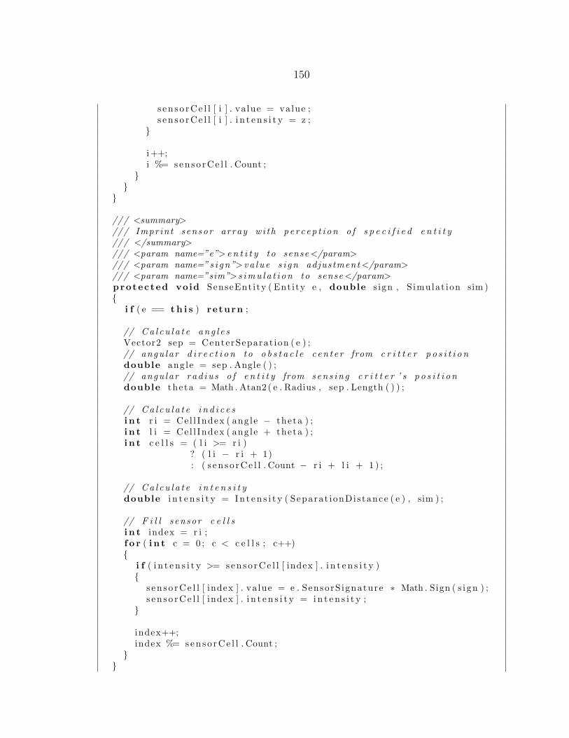
150
s en s o rCe l l [ i ] . va lue = value ;s e n s o rCe l l [ i ] . i n t e n s i t y = z ;
}
i++;i %= sen s o rCe l l . Count ;
}}
}
/// <summary>/// Imprint sensor array wi th p e r c ep t i on o f s p e c i f i e d e n t i t y/// </summary>/// <param name=”e”> e n t i t y to sense </param>/// <param name=”s i gn”>va l u e s i gn adjustment </param>/// <param name=”sim”> s imu l a t i on to sense </param>protected void SenseEnt i ty ( Entity e , double s ign , S imulat ion sim ){
i f ( e == t h i s ) return ;
// Ca l c u l a t e ang l e sVector2 sep = CenterSeparat ion ( e ) ;// angu lar d i r e c t i o n to o b s t a c l e c en t e r from c r i t t e r p o s i t i o ndouble ang le = sep . Angle ( ) ;// angu lar r ad i u s o f e n t i t y from sens in g c r i t t e r ’ s p o s i t i o ndouble theta = Math . Atan2 ( e . Radius , sep . Length ( ) ) ;
// Ca l c u l a t e i n d i c e si n t r i = Ce l l Index ( ang le − theta ) ;i n t l i = Ce l l Index ( ang le + theta ) ;i n t c e l l s = ( l i >= r i )
? ( l i − r i + 1): ( s en s o rCe l l . Count − r i + l i + 1 ) ;
// Ca l c u l a t e i n t e n s i t ydouble i n t e n s i t y = In t e n s i t y ( Separat ionDis tance ( e ) , sim ) ;
// F i l l s ensor c e l l si n t index = r i ;f o r ( i n t c = 0 ; c < c e l l s ; c++){
i f ( i n t e n s i t y >= sen s o rCe l l [ index ] . i n t e n s i t y ){
s en s o rCe l l [ index ] . va lue = e . SensorS ignature ∗ Math . Sign ( s i gn ) ;s e n s o rCe l l [ index ] . i n t e n s i t y = i n t e n s i t y ;
}
index++;index %= sen s o rCe l l . Count ;
}}
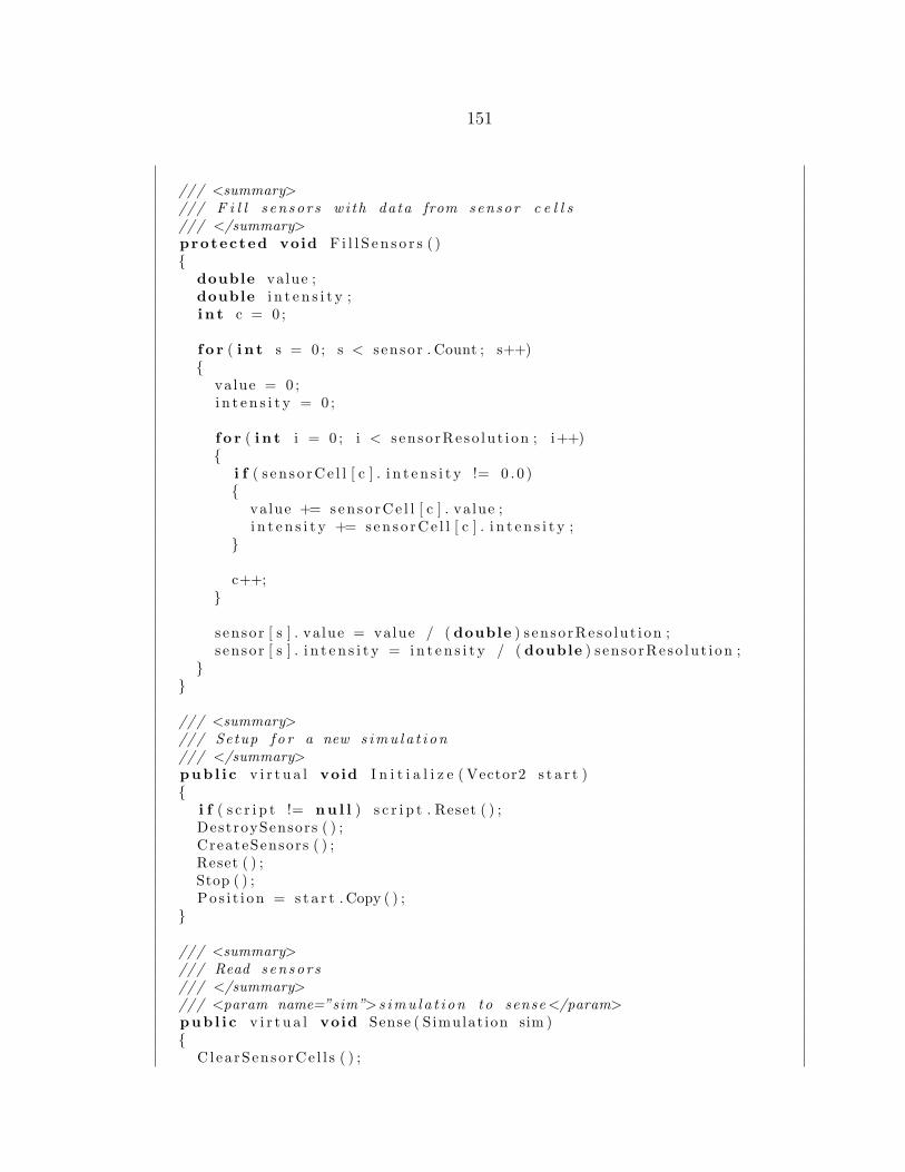
151
/// <summary>/// F i l l s en so r s wi th data from sensor c e l l s/// </summary>protected void F i l l S e n s o r s ( ){
double value ;double i n t e n s i t y ;i n t c = 0 ;
f o r ( i n t s = 0 ; s < s enso r . Count ; s++){
value = 0 ;i n t e n s i t y = 0 ;
f o r ( i n t i = 0 ; i < s en so rReso lu t i on ; i++){
i f ( s en s o rCe l l [ c ] . i n t e n s i t y != 0 . 0 ){
value += sen s o rCe l l [ c ] . va lue ;i n t e n s i t y += sen s o rCe l l [ c ] . i n t e n s i t y ;
}
c++;}
s enso r [ s ] . va lue = value / ( double ) s en so rReso lu t i on ;s enso r [ s ] . i n t e n s i t y = i n t e n s i t y / ( double ) s en so rReso lu t i on ;
}}
/// <summary>/// Setup f o r a new s imu l a t i on/// </summary>pub l i c v i r t u a l void I n i t i a l i z e ( Vector2 s t a r t ){
i f ( s c r i p t != nu l l ) s c r i p t . Reset ( ) ;DestroySensors ( ) ;CreateSensors ( ) ;Reset ( ) ;Stop ( ) ;Po s i t i on = s t a r t . Copy ( ) ;
}
/// <summary>/// Read s en so r s/// </summary>/// <param name=”sim”> s imu l a t i on to sense </param>pub l i c v i r t u a l void Sense ( S imulat ion sim ){
Clea rSenso rCe l l s ( ) ;

152
i f ( sim . F i e ld . V i s ib l eWa l l s ) SenseWalls (−1.0 , sim ) ;
f o r each ( Obstac le o in sim . F i e ld . Obstac le )SenseEnt i ty ( o , 1 . 0 , sim ) ;
SenseEnt i ty ( sim . Fox , 1 . 0 , sim ) ;SenseEnt i ty ( sim . Rabbit , 1 . 0 , sim ) ;
F i l l S e n s o r s ( ) ;}
}
Listing B.13: Selections from Critter.cs
/// <summary>/// S imu la t i on c l a s s/// By : Sam Gardner/// 05−23−2008/// Modi f i ed : 12−16−2008/// </summary>pub l i c c l a s s Simulat ion{
pr i va t e RandomGenerator rand ;
pr i va t e List<s t r i ng > comment ;
pr i va t e Simulat ionReplay rep lay ;
pr i va t e s t r i n g name ;
pr i va t e s t r i n g f i t n e s sFunc t i on ;pr i va t e s t r i n g terminat ionFunct ion ;
pr i va t e double f unne lD i s t anceSca l a r ;pr i va t e double f unne lAcce lS ca l a r ;pr i va t e double f unne lEps i l on ;pr i va t e double proximityThreshold ;pr i va t e List<ProximityFie ld> graduatedProximityFie ld ;
pr i va t e double t a rg e tSco r e ;pr i va t e i n t ta rge tStep ;
pr i va t e Fie ld f i e l d ;pr i va t e Cr i t t e r fox ;pr i va t e Cr i t t e r rabb i t ;
pr i va t e Stat d i s t anc e ;pr i va t e Stat approach ;
153
pr i va t e Stat speed ;pr i va t e Stat a c c e l ;
pr i va t e double scoreQuickCapture ;pr i va t e double scoreMinDistance ;pr i va t e double s co r eD i s c r e t eProx im i ty ;pr i va t e double scoreApproach ;pr i va t e double scoreDiscreteApproach ;
pr i va t e double scoreFunne lDis tance ;pr i va t e double s co r eFunne lAcce l e ra t i on ;
pr i va t e double s co reMutua l lyExc lus iveDi sc r e t eProx imi ty ;pr i va t e double scoreMutua l lyExc lus iveDiscreteApproach ;
pr i va t e double scoreGraduatedProximity ;pr i va t e double scoreGraduatedApproach ;
pr i va t e i n t s tep ;pr i va t e bool capture ;pr i va t e bool i n i t i a l i z e d ;pr i va t e bool f i n i s h e d ;
/// <summary>/// Create a new fox r a b b i t s imu l a t i on/// </summary>pub l i c Simulat ion ( ){
rand = new RandomGenerator ( ) ;
comment = new List<s t r i ng >() ;
r ep lay = nu l l ;
name = ”Simulat ion ” ;
f i t n e s sFunc t i on = ”” ;terminat ionFunct ion = ”Step” ;
f unne lD i s t anceSca l a r = 0 . 5 ;f unne lAcc e lS ca l a r = 0 . 0 0 2 ;funne lEps i l on = 0 . 0 0 1 ;proximityThreshold = 2 . 0 ;graduatedProximityFie ld = new List<ProximityFie ld >() ;graduatedProximityFie ld .Add(new ProximityFie ld ( 0 . 0 , 1 . 0 0 ) ) ;graduatedProximityFie ld .Add(new ProximityFie ld ( 1 . 0 , 0 . 9 5 ) ) ;graduatedProximityFie ld .Add(new ProximityFie ld ( 2 . 0 , 0 . 9 0 ) ) ;graduatedProximityFie ld .Add(new ProximityFie ld ( 3 . 0 , 0 . 8 5 ) ) ;graduatedProximityFie ld .Add(new ProximityFie ld ( 4 . 0 , 0 . 8 0 ) ) ;graduatedProximityFie ld .Add(new ProximityFie ld ( 5 . 0 , 0 . 7 5 ) ) ;
154
t a r g e tSco r e = 100 . 0 ;ta rge tStep = 500 ;
f i e l d = new Fie ld ( ) ;Fox = new NeuralNetworkCritter ( ) ;Rabbit = new S ta t i ona ryCr i t t e r ( ) ;
d i s t anc e = new Stat ( ) ;approach = new Stat ( ) ;speed = new Stat ( ) ;a c c e l = new Stat ( ) ;
}
/// <summary>/// Reset s t a t s f o r a new s imu l a t i on/// </summary>pr i va t e void I n i t i a l i z e S t a t s ( ){
d i s t anc e . Clear ( ) ;approach . Clear ( ) ;speed . Clear ( ) ;a c c e l . Clear ( ) ;
}
/// <summary>/// Record s t a t s from cur r en t s imu l a t i on s t e p/// </summary>pr i va t e void UpdateStats ( ){
d i s t anc e .Add( fox . Separat ionDis tance ( rabb i t ) ) ;approach .Add( ( s tep > 0) ? −d i s t anc e . Der iva t iv e : 0 . 0 ) ;speed .Add( fox . Ve loc i ty . Length ( ) ) ;a c c e l .Add( fox . Acce l e r a t i on . Length ( ) ) ;
}
/// <summary>/// Get cu r r en t f o x s core/// </summary>pub l i c double Score ( ){
double s co r e = 0 . 0 ;
switch ( f i t n e s sFunc t i on . ToLower ( ) ){
// o v e r l y complex (06−03−2008)// [ 0 . 0 , 1 00 . 0 ]// 50% f o r speed ( awarded upon cap ture )// 25% f o r d i s t a n c e ( recomputed each time s t e p )// 25% f o r approach ( awarded per t ime s t e p )
155
case ” o r i g i n a l ” :s c o r e += 50 .0 ∗ scoreQuickCapture ;s c o r e += 25 .0 ∗ scoreMinDistance ;i f ( scoreApproach > 0 . 0 ) s co r e += 25 .0 ∗ scoreApproach ;break ;
// approach awarded (06−09−2008)// [ 0 . 0 , 1 00 . 0 ]// 100% f o r cap ture (no−ad jus tment s )// 50% f o r approach// ( s t a r t i n g wi th 0% and i n c r e a s i n g wi th each time s t e p )case ” d i s c r e t e−approach” :
i f ( capture )s co r e = 100 . 0 ;
e l s ei f ( scoreDiscreteApproach > 0 . 0 )
s co r e += 50 .0 ∗ scoreDiscreteApproach ;break ;
// approach awarded and n e g a t i v e approach punished// [ 0 . 0 , 1 00 . 0 ]// 100 f o r cap ture// 80 f o r approach// ( s t a r t i n g a t 40 and changing wi th each t ime s t e p )case ” b i d i r e c t i o n a l−approach” :
s co r e = capture ? 100 .0 : ( 40 . 0 + (40 . 0 ∗ scoreApproach ) ) ;break ;
// approach awarded and n e g a t i v e approach punished (06−14−2008)// a l s o used in wa l l− l e s s and x g a l l e r y s imu l a t i on s// [ 0 . 0 , 1 00 . 0 ]// 100% f o r cap ture (no−ad jus tment s )// 80% f o r approach// ( s t a r t i n g wi th 40% and changing wi th each time s t e p )case ” b i d i r e c t i o n a l−d i s c r e t e−approach” :
s co r e = capture ? 100 .0: ( 40 . 0 + (40 . 0 ∗ scoreDiscreteApproach ) ) ;
break ;
// i n c e n t i v e f o r approach l e a d i n g to l a r g e award f o r// main ta in ing prox imi t y// bonus g i v en f o r cap ture (06−20−2008)// used in l o c a l i t y s imu l a t i on// [ 0 . 0 , 1 00 . 0 ]// 10% f o r cap ture ( awarded upon cap ture )// 60% f o r p rox imi t y ( accumulated wi th each time s t e p )// 30% f o r approach// ( s t a r t i n g wi th 15% and changing wi th each time s t e p )case ” d i s c r e t e−proximity−and−approach” :
i f ( capture ) s co r e += 10 . 0 ;s c o r e += 60 .0 ∗ s co r eD i s c r e t eProx im i ty ;
156
s co r e += (15 . 0 + (15 . 0 ∗ scoreDiscreteApproach ) ) ;break ;
// accumula tes h i gh p r e c i s i o n score reward ing// non− l i n e a r c l o s e n e s s ( f unne l ) (7−18−2008)// [ 0 . 0 , +i n f ]// due to ep s i l on , p r a c t i c a l upper l i m i t i s// f unne lD i s t an c eSca l a r ∗ f i e l d . MaxSeparat ionDistance / e p s i l o n// t o t a l : about 70 ,711 f o r kd = 0 .5 , e p s i l o n = 0.001// and 100 x 100 f i e l dcase ” funnel−di s tance−only ” :
s co r e = scoreFunne lDis tance ;break ;
// accumula tes h i gh p r e c i s i o n score reward ing// non− l i n e a r c l o s e n e s s ( f unne l ) and low a c c e l e r a t i o n (7−18−2008)// [ 0 . 0 , +i n f ]// due to ep s i l on , p r a c t i c a l upper d i s t a n c e score l i m i t i s// f unne lD i s t an c eSca l a r ∗ f i e l d . MaxSeparat ionDistance / e p s i l o n// the p r a c t i c a l upper a c c e l e r a t i o n score l i m i t i s// f unne lAc c e l S c a l a r ∗ f o x . MaxAccel / e p s i l o n// t o t a l : about 70 ,713 f o r ka = 0.002 , e p s i l o n = 0.001 ,// 100 x 100 f i e l d , and maxAccel = 1 .0case ” funnel−di s tance−and−a c c e l e r a t i o n ” :
s co r e = scoreFunne lDis tance + sco reFunne lAcce l e ra t i on ;break ;
// po i n t s accumulated each t ime s t e p f o r e i t h e r// d i s c r e t e p rox imi t y or d i s c r e t e approach (07−21−2008)// [ 0 . 0 , 1 00 . 0 ]// 100% max f o r approach ( accumulated wi th each time s t e p )// 100% max f o r p rox imi t y ( accumulated wi th each time s t e p )// no more than 100% t o t a lcase ” d i s c r e t e−approach−or−proximity ” :
s co r e = 100 .0∗ ( s co reMutua l lyExc lus iveDi sc r e t eProx imi ty
+ scoreMutua l lyExc lus iveDiscreteApproach ) ;break ;
// po i n t s accumulated each t ime s t e p f o r e i t h e r// d i s c r e t e p rox imi t y or d i s c r e t e approach (07−30−2008)// [ 0 . 0 , 1 00 . 0 ]// 6 l e v e l s o f p rox imi t y// 100% max f o r o v e r l a p// 95% max f o r w i t h i n 1 .0// 90% max f o r w i t h i n 2 .0// 85% max f o r w i t h i n 3 .0// 80% max f o r w i t h i n 4 .0// 75% max f o r w i t h i n 5 .0// 50% max f o r p rox im i t y// no more than 100% t o t a l
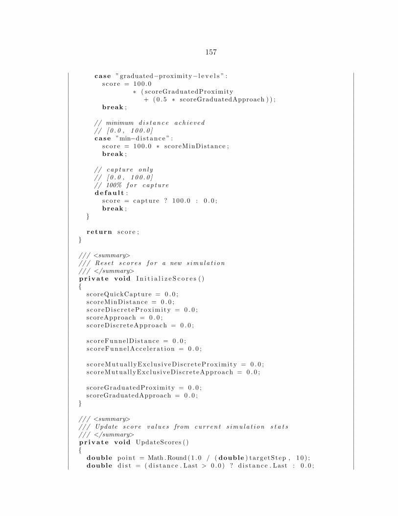
157
case ”graduated−proximity− l e v e l s ” :s c o r e = 100 .0
∗ ( scoreGraduatedProximity+ (0 . 5 ∗ scoreGraduatedApproach ) ) ;
break ;
// minimum d i s t an c e ach i e v ed// [ 0 . 0 , 1 00 . 0 ]case ”min−d i s t anc e ” :
s co r e = 100 .0 ∗ scoreMinDistance ;break ;
// cap ture on ly// [ 0 . 0 , 1 00 . 0 ]// 100% f o r cap turede f au l t :
s c o r e = capture ? 100 .0 : 0 . 0 ;break ;
}
return s co r e ;}
/// <summary>/// Reset s c o r e s f o r a new s imu l a t i on/// </summary>pr i va t e void I n i t i a l i z e S c o r e s ( ){
scoreQuickCapture = 0 . 0 ;scoreMinDistance = 0 . 0 ;s co r eD i s c r e t eProx im i ty = 0 . 0 ;scoreApproach = 0 . 0 ;scoreDiscreteApproach = 0 . 0 ;
scoreFunne lDis tance = 0 . 0 ;s co r eFunne lAcce l e ra t i on = 0 . 0 ;
s co reMutua l lyExc lus iveDi sc r e t eProx imi ty = 0 . 0 ;scoreMutua l lyExc lus iveDiscreteApproach = 0 . 0 ;
scoreGraduatedProximity = 0 . 0 ;scoreGraduatedApproach = 0 . 0 ;
}
/// <summary>/// Update s core v a l u e s from cur r en t s imu l a t i on s t a t s/// </summary>pr i va t e void UpdateScores ( ){
double po int = Math . Round ( 1 . 0 / ( double ) targetStep , 1 0 ) ;double d i s t = ( d i s t ance . Last > 0 . 0 ) ? d i s t anc e . Last : 0 . 0 ;
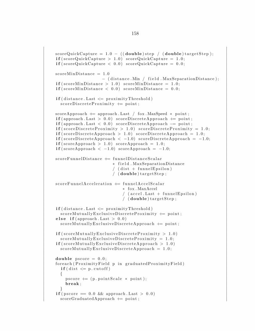
158
scoreQuickCapture = 1 .0 − ( ( double ) s tep / ( double ) ta rge tStep ) ;i f ( scoreQuickCapture > 1 . 0 ) scoreQuickCapture = 1 . 0 ;i f ( scoreQuickCapture < 0 . 0 ) scoreQuickCapture = 0 . 0 ;
scoreMinDistance = 1 .0− ( d i s t anc e . Min / f i e l d . MaxSeparationDistance ) ;
i f ( scoreMinDistance > 1 . 0 ) scoreMinDistance = 1 . 0 ;i f ( scoreMinDistance < 0 . 0 ) scoreMinDistance = 0 . 0 ;
i f ( d i s t anc e . Last <= proximityThreshold )s co r eD i s c r e t eProx im i ty += point ;
scoreApproach += approach . Last / fox . MaxSpeed ∗ po int ;i f ( approach . Last > 0 . 0 ) scoreDiscreteApproach += point ;i f ( approach . Last < 0 . 0 ) scoreDiscreteApproach −= point ;i f ( s co r eD i s c r e t eProx im i ty > 1 . 0 ) s co r eD i s c r e t eProx imi ty = 1 . 0 ;i f ( scoreDiscreteApproach > 1 . 0 ) scoreDiscreteApproach = 1 . 0 ;i f ( scoreDiscreteApproach < −1.0) scoreDiscreteApproach = −1.0;i f ( scoreApproach > 1 . 0 ) scoreApproach = 1 . 0 ;i f ( scoreApproach < −1.0) scoreApproach = −1.0;
scoreFunne lDis tance += funne lD i s t anceSca l a r∗ f i e l d . MaxSeparationDistance/ ( d i s t + funne lEps i l on )/ ( double ) ta rge tStep ;
s co r eFunne lAcce l e ra t i on += funne lAcc e lS ca l a r∗ fox . MaxAccel/ ( a c c e l . Last + funne lEps i l on )/ ( double ) ta rge tStep ;
i f ( d i s t anc e . Last <= proximityThreshold )s co reMutua l lyExc lus iveDi sc r e t eProx imi ty += point ;
e l s e i f ( approach . Last > 0 . 0 )scoreMutua l lyExc lus iveDiscreteApproach += point ;
i f ( s co reMutua l lyExc lus iveDi sc r e t eProx imi ty > 1 . 0 )s co reMutua l lyExc lus iveDi sc r e t eProx imi ty = 1 . 0 ;
i f ( scoreMutua l lyExc lus iveDiscreteApproach > 1 . 0 )scoreMutua l lyExc lus iveDiscreteApproach = 1 . 0 ;
double pscore = 0 . 0 ;f o r each ( Prox imityFie ld p in graduatedProximityFie ld )
i f ( d i s t <= p . c u t o f f ){
pscore += (p . po in tSca l e ∗ po int ) ;break ;
}i f ( pscore == 0.0 && approach . Last > 0 . 0 )
scoreGraduatedApproach += point ;

159
scoreGraduatedProximity += pscore ;
i f ( scoreGraduatedProximity > 1 . 0 ) scoreGraduatedProximity = 1 . 0 ;i f ( scoreGraduatedApproach > 1 . 0 ) scoreGraduatedApproach = 1 . 0 ;
}
/// <summary>/// Detec t and r e a c t to c o l l i s i o n s between f o x / r a b b i t and environment/// </summary>pr i va t e void Co l l i s i o nCo r r e c t i o n ( ){
fox . Co l l ideWal l s ( t h i s ) ;r abb i t . Co l l ideWal l s ( t h i s ) ;f o r each ( Obstac le o in f i e l d . Obstac le ){
fox . Co l l i d e ( o ) ;r abb i t . Co l l i d e ( o ) ;
}
fox . Co l l i s i onAd ju s t ( ) ;r abb i t . Co l l i s i onAd ju s t ( ) ;
i f ( fox . C o l l i s i o n ( rabb i t ) < 1 . 0 ) capture = true ;}
/// <summary>/// Reset t he s imu l a t i on f o r another run/// </summary>pub l i c void Reset ( ){
I n i t i a l i z e C r i t t e r ( rabb i t ) ;i f ( fox . S t a r tRe l a t i v e ) fox . S ta r t = rabb i t . Po s i t i on . Copy ( ) ;I n i t i a l i z e C r i t t e r ( fox ) ;
fox . Sense ( t h i s ) ;r abb i t . Sense ( t h i s ) ;
s t ep = 0 ;capture = f a l s e ;f i n i s h e d = f a l s e ;
i f ( fox . Overlapping ( rabb i t ) ) capture = true ;
I n i t i a l i z e S t a t s ( ) ;I n i t i a l i z e S c o r e s ( ) ;r ep lay = new Simulat ionReplay ( ) ;r ep lay . I n i t i a l i z e ( t h i s ) ;
i n i t i a l i z e d = true ;}

160
/// <summary>/// Set up s p e c i f i e d c r i t t e r f o r a new s imu l a t i on/// </summary>pr i va t e void I n i t i a l i z e C r i t t e r ( C r i t t e r c ){
// Find s t a r t i n g p o s i t i o ni f ( c . StartAnywhere ){
c . S ta r t . Zero ( ) ;c . StartRange = new Vector2 ( f i e l d . Width / 2 .0 − c . Radius ,
f i e l d . Height / 2 .0 − c . Radius ) ;}c . I n i t i a l i z e ( c . S t a r tPo s i t i on ( ) ) ;
// Correc t f o r i n i t i a l o v e r l a pc . OverlapCorrectWal ls ( t h i s ) ;f o r each ( Obstac le o in f i e l d . Obstac le )
c . Over lapCorrect ( o ) ;}
/// <summary>/// Run the s imu l a t i on f o r a s i n g l e t ime s t e p/// </summary>pub l i c void RunStep ( ){
i f ( ! f i n i s h e d ){
i f ( ! i n i t i a l i z e d ){
Reset ( ) ;}e l s e{
fox . ComputeNextAction ( t h i s ) ;r abb i t . ComputeNextAction ( t h i s ) ;
UpdateStats ( ) ;UpdateScores ( ) ;r ep lay . Update ( t h i s ) ;
Co l l i s i o nCo r r e c t i o n ( ) ;
fox .Move ( ) ;r abb i t .Move ( ) ;
fox . Sense ( t h i s ) ;r abb i t . Sense ( t h i s ) ;
s t ep++;
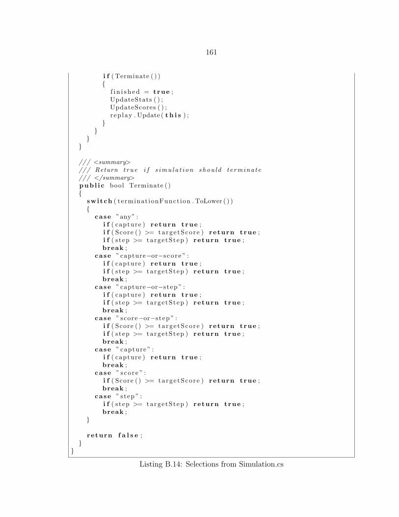
161
i f ( Terminate ( ) ){
f i n i s h e d = true ;UpdateStats ( ) ;UpdateScores ( ) ;r ep lay . Update ( t h i s ) ;
}}
}}
/// <summary>/// Return t rue i f s imu l a t i on shou l d t e rmina te/// </summary>pub l i c bool Terminate ( ){
switch ( terminat ionFunct ion . ToLower ( ) ){
case ”any” :i f ( capture ) return true ;i f ( Score ( ) >= targe tSco r e ) return true ;i f ( s tep >= targe tStep ) return true ;break ;
case ” capture−or−s co r e ” :i f ( capture ) return true ;i f ( s tep >= targe tStep ) return true ;break ;
case ” capture−or−s tep ” :i f ( capture ) return true ;i f ( s tep >= targe tStep ) return true ;break ;
case ” score−or−s tep ” :i f ( Score ( ) >= targe tSco r e ) return true ;i f ( s tep >= targe tStep ) return true ;break ;
case ” capture ” :i f ( capture ) return true ;break ;
case ” s co r e ” :i f ( Score ( ) >= targe tSco r e ) return true ;break ;
case ” step ” :i f ( s tep >= targe tStep ) return true ;break ;
}
return f a l s e ;}
}
Listing B.14: Selections from Simulation.cs
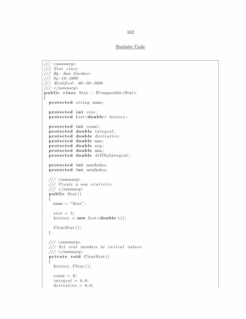
162
Statistic Code
/// <summary>/// S t a t c l a s s/// By : Sam Gardner/// 04−10−2008/// Modi f i ed : 06−20−2008/// </summary>pub l i c c l a s s Stat : IComparable<Stat>{
protected s t r i n g name ;
protected i n t s i z e ;protected List<double> h i s t o r y ;
protected i n t count ;protected double i n t e g r a l ;protected double d e r i v a t i v e ;protected double max ;protected double avg ;protected double min ;protected double d i f f S q I n t e g r a l ;
protected i n t maxIndex ;protected i n t minIndex ;
/// <summary>/// Create a new s t a t i s t i c/// </summary>pub l i c Stat ( ){
name = ”Stat ” ;
s i z e = 5 ;h i s t o r y = new List<double >() ;
C learStat ( ) ;}
/// <summary>/// Set s t a t members to i n i t i a l v a l u e s/// </summary>pr i va t e void ClearStat ( ){
h i s t o r y . Clear ( ) ;
count = 0 ;i n t e g r a l = 0 . 0 ;d e r i v a t i v e = 0 . 0 ;
163
max = 0 . 0 ;avg = 0 . 0 ;min = 0 . 0 ;d i f f S q I n t e g r a l = 0 . 0 ;
maxIndex = −1;minIndex = −1;
}
/// <summary>/// Get cu r r en t va r i ance o f a l l v a l u e s/// accounted f o r by t h i s s t a t i s t i c/// </summary>pub l i c double Variance{
get { return d i f f S q I n t e g r a l / ( double ) count ; }}
/// <summary>/// Get cu r r en t s tandard d e v i a t i o n o f a l l v a l u e s/// accounted f o r by t h i s s t a t i s t i c/// </summary>pub l i c v i r t u a l double StdDev{
get { return Math . Sqrt ( Variance ) ; }}
/// <summary>/// Ca l c u l a t e t he in s t an t aneou s running average f o r the s t a t i s t i c/// acc ro s s t he s p e c i f i e d number o f data p o i n t s/// <para>po i n t s must be l e s s than or e qua l to h i s t o r y s i z e </para>/// </summary>/// <param name=”po i n t s”>number o f v a l u e s to average </param>pub l i c v i r t u a l double RunningAvg ( i n t po in t s ){
double sum = 0 . 0 ;i n t p = 0 ;whi le (p < po in t s && p < h i s t o r y . Count ){
sum += h i s t o r y [ h i s t o r y . Count − 1 − p ] ;p++;
}
return sum / ( double ) po in t s ;}
/// <summary>/// Add a new va l u e to the s t a t i s t i c c a l c u l a t i o n s/// </summary>/// <param name=”va l u e”>va l u e to record </param>

164
pub l i c v i r t u a l void Add( double value ){
double d i f f ;double l a s t = Last ;
h i s t o r y .Add( value ) ;i f ( h i s t o r y . Count > s i z e ) h i s t o r y . RemoveAt ( 0 ) ;
i n t e g r a l += value ;d e r i v a t i v e = value − l a s t ;
i f ( va lue > max | | count == 0){
max = value ;maxIndex = count ;
}i f ( va lue < min | | count == 0){
min = value ;minIndex = count ;
}
count++;
avg = i n t e g r a l / ( double ) count ;d i f f = value − avg ;d i f f S q I n t e g r a l += d i f f ∗ d i f f ;
}}
Listing B.15: Selections from Stat.cs
/// <summary>/// S t a t L i s t c l a s s/// By : Sam Gardner/// 04−10−2008/// Modi f i ed : 01−06−2009/// </summary>pub l i c c l a s s S ta tL i s t : IEnumerable<Stat>{
pr i va t e List<Stat> s t a t ;
/// <summary>/// Create a new s t a t l i s t/// </summary>pub l i c S ta tL i s t ( ){
s t a t = new List<Stat >() ;

165
}
/// <summary>/// Add s t a t i s t i c s f o r each va l u e o f a s t a t i s t i c/// wi th the g i v en name/// <para>no data i s recorded </para>/// </summary>/// <param name=”name”>base name</param>pub l i c void AddMeta( s t r i n g name){
Add(name + ”−max” ) ;Add(name + ”−avg” ) ;Add(name + ”−min” ) ;Add(name + ”−stddev ” ) ;Add(name + ”−var iance ” ) ;Add(name + ”−d e r i v a t i v e ” ) ;
}
/// <summary>/// Add s t a t i s t i c s f o r each va l u e o f a l l s t a t i s t i c s in l i s t/// <para>no data i s recorded </para>/// </summary>/// <param name=” l i s t ”> s t a t l i s t </param>pub l i c void AddMeta( S t a tL i s t l i s t ){
f o r each ( Stat s in l i s t )AddMeta( s ) ;
}
/// <summary>/// Record s t a t i s t i c s f o r each va l u e o f a s t a t i s t i c/// wi th a d i f f e r e n t name/// <para> s t a t i s t i c s are c r ea t e d i f t h ey don ’ t e x i s t </para>/// </summary>/// <param name=”s”> s t a t i s t i c to sample</param>/// <param name=”name”>new s t a t name</param>pub l i c void RecordMetaAs ( Stat s , s t r i n g name){
t h i s [ name + ”−max” ] . Add( s .Max ) ;t h i s [ name + ”−avg” ] . Add( s . Avg ) ;t h i s [ name + ”−min” ] . Add( s . Min ) ;t h i s [ name + ”−stddev ” ] . Add( s . StdDev ) ;t h i s [ name + ”−var iance ” ] . Add( s . Variance ) ;t h i s [ name + ”−d e r i v a t i v e ” ] . Add( s . Der iva t i ve ) ;
}}
Listing B.16: Selections from StatList.cs
Recommended