Exploring, exploiting and evolving diversity of aquaticecosystem models: a community perspective
Annette B. G. Janssen . George B. Arhonditsis . Arthur Beusen . Karsten Bolding .
Louise Bruce . Jorn Bruggeman . Raoul-Marie Couture . Andrea S. Downing .
J. Alex Elliott . Marieke A. Frassl . Gideon Gal . Daan J. Gerla . Matthew R. Hipsey .
Fenjuan Hu . Stephen C. Ives . Jan H. Janse . Erik Jeppesen . Klaus D. Johnk .
David Kneis . Xiangzhen Kong . Jan J. Kuiper . Moritz K. Lehmann . Carsten Lemmen .
Deniz Ozkundakci . Thomas Petzoldt . Karsten Rinke . Barbara J. Robson . Rene Sachse .
Sebastiaan A. Schep . Martin Schmid . Huub Scholten . Sven Teurlincx . Dennis Trolle .
Tineke A. Troost . Anne A. Van Dam . Luuk P. A. Van Gerven . Mariska Weijerman .
Scott A. Wells . Wolf M. Mooij
Received: 3 June 2015 / Accepted: 14 September 2015 / Published online: 29 September 2015
� The Author(s) 2015. This article is published with open access at Springerlink.com
Abstract Here, we present a community perspective
on how to explore, exploit and evolve the diversity in
aquatic ecosystem models. These models play an
important role in understanding the functioning of
aquatic ecosystems, filling in observation gaps and
developing effective strategies for water quality
management. In this spirit, numerous models have
been developed since the 1970s. We set off to explore
model diversity by making an inventory among 42
aquatic ecosystem modellers, by categorizing the
resulting set of models and by analysing them for
diversity. We then focus on how to exploit model
diversity by comparing and combining different
aspects of existing models. Finally, we discuss how
model diversity came about in the past and could
evolve in the future. Throughout our study, we use
Handling Editor: Piet Spaak.
Electronic supplementary material The online version ofthis article (doi:10.1007/s10452-015-9544-1) contains supple-mentary material, which is available to authorized users.
A. B. G. Janssen � J. H. Janse � X. Kong �J. J. Kuiper � S. Teurlincx � L. P. A. Van Gerven �W. M. Mooij (&)
Department of Aquatic Ecology, Netherlands Institute of
Ecology, PO Box 50, 6700 AB Wageningen,
The Netherlands
e-mail: [email protected]
A. B. G. Janssen � J. J. Kuiper � L. P. A. Van Gerven �M. Weijerman � W. M. Mooij
Department of Aquatic Ecology and Water Quality
Management, Wageningen University, PO Box 47,
6700 AA Wageningen, The Netherlands
G. B. Arhonditsis
Ecological Modelling Laboratory, Department of Physical
and Environmental Sciences, University of Toronto,
Toronto, ON M1C 1A4, Canada
A. Beusen � J. H. JansePBL Netherlands Environmental Assessment Agency,
PO Box 303, 3720 AH Bilthoven, The Netherlands
K. Bolding � F. Hu � E. Jeppesen � D. TrolleDepartment of Bioscience and Arctic Centre, Aarhus
University, PO Box 314, 8600 Silkeborg, Denmark
K. Bolding � E. Jeppesen � D. TrolleSino-Danish Center for Education and Research (SDC),
UCAS, Beijing, People’s Republic of China
L. Bruce � M. R. Hipsey
Aquatic Ecodynamics Group, School of Earth and
Environment, The University of Western Australia, Perth,
WA 6009, Australia
123
Aquat Ecol (2015) 49:513–548
DOI 10.1007/s10452-015-9544-1
analogies from biodiversity research to analyse and
interpret model diversity. We recommend to make
models publicly available through open-source poli-
cies, to standardize documentation and technical
implementation of models, and to compare models
through ensemble modelling and interdisciplinary
approaches. We end with our perspective on how the
field of aquatic ecosystem modelling might develop in
the next 5–10 years. To strive for clarity and to
improve readability for non-modellers, we include a
glossary.
Keywords Water quality � Ecology �Geochemistry �Hydrology � Hydraulics � Hydrodynamics � Physicalenvironment � Socio-economics � Model availability �Standardization � Linking
Introduction
The societal niche for aquatic ecosystem models:
developing short-term and long-term management
strategies
Aquatic ecosystems provide a range of ecosystem
services (Finlayson et al. 2005), in particular by being
sources and sinks for natural resources and
anthropogenic substances. For example, as a source,
they provide water for drinking, irrigation, hydro-
power and industrial processes. Moreover, they
provide many food products. More recently, their
aesthetic and recreational value has been recognized
with associated health benefits. Aquatic ecosystems
also act as a sink for various substances, including
sewage, agricultural run-off, discharge from impound-
ments, industrial waste and thermally polluted water.
Equally important, they provide a critical habitat for
organisms that form an important part of the biodi-
versity. Each of the anthropogenic and natural source
functions puts specific requirements on the quality of
the aquatic ecosystem (Postel and Richter 2003;
Keeler et al. 2012). At the same time, these quality
requirements can be hampered by both the source
(through overexploitation) and the sink (through
pollution) functions of the aquatic ecosystem. Aquatic
ecosystem models (hereafter referred to as AEMs)
frequently play a role in quantifying ecosystem
services and developing strategies for water quality
management (Jørgensen 2010; Mooij et al. 2010). The
AEMs used for this purpose are often engineering-
oriented based on accepted theory and methodology
for routine applications. Engineering models may be
complex and linked to one another, but components
are always tested. Using projections and scenario
J. Bruggeman
Plymouth Marine Laboratory, Prospect Place, The Hoe,
Plymouth PL1 3DH, UK
R.-M. Couture
Norwegian Institute for Water Research, Gaustadalleen
21, 0349 Oslo, Norway
R.-M. Couture
Ecohydrology Group, Department of Earth and
Environmental Sciences, University of Waterloo, 200
University Ave. W, Waterloo, ON N2L 3G1, Canada
A. S. Downing
Stockholm Resilience Centre, Stockholm University,
Stockholm, Sweden
J. Alex Elliott
Centre for Ecology and Hydrology, Lancaster, Library
Avenue, Bailrigg, Lancashire LA1 4AP, UK
M. A. Frassl � K. RinkeDepartment of Lake Research, UFZ, Helmholtz Centre for
Environmental Research, Bruckstrasse 3A,
39114 Magdeburg, Germany
G. Gal
Kinneret Limnological Laboratory, IOLR, PO Box 447,
14950 Migdal, Israel
D. J. Gerla
Department of Ecosystem Studies, Royal Netherlands
Institute for Sea Research (NIOZ-Yerseke), PO Box 140,
4400 AC Yerseke, The Netherlands
F. Hu
Department of Biology, University of Southern Denmark,
Odense M., Denmark
S. C. Ives
Centre for Ecology and Hydrology, Bush Estate,
Penicuik, Midlothian EH26 0QB, UK
S. C. Ives
School of GeoSciences, University of Edinburgh, Crew
Building, The King’s Buildings, Alexander Crum Brown
Road, Edinburgh EH9 3FF, UK
K. D. Johnk � B. J. RobsonCSIRO Land and Water Flagship,
GPO Box 1666, Canberra, ACT 2601, Australia
514 Aquat Ecol (2015) 49:513–548
123
analyses, engineering-oriented AEMs can assess the
various source and sink functions to help optimize and
understand aquatic ecosystem function in terms of
human and conservation needs. For example, AEMs
have been applied as management tools to evaluate the
efficiency of eutrophication mitigation strategies, to
understand oceanic dynamics (e.g. the global carbon
cycle), and to predict biotic responses to climate
change (Arhonditsis and Brett 2004). AEMs can also
be used for near real-time modelling and forecasting to
facilitate immediate management decisions on, for
instance, the shutdown of drinking water intakes
(Huang et al. 2012; Silva et al. 2014) or the suitability
of water for swimming (Ibelings et al. 2003).
The scientific niche for AEMs: advancement
of theory
A strong scientific motivation for the development of
AEMs is to encapsulate and improve our understand-
ing of aquatic ecosystems. For instance, scientific
AEMs can help to close mass balances of essential
elements such as carbon, nitrogen and phosphorus and
thereby allow quantifying the role of aquatic systems
in national and global carbon and nutrient budgets
(Robson et al. 2008; Harrison et al. 2012). Keeping
track of mass balances can also provide help in
answering stoichiometric questions (Giordani et al.
2008; Li et al. 2014). Additionally, scientific AEMs
can help untangle the feedbacks between aquatic
biodiversity and aquatic ecosystem functioning
(Bruggeman and Kooijman 2007), and also achieve
an integrated ecosystem health assessment (Xu et al.
2001). Yet another timely research topic studied with
models is assessing the resilience of ecosystems to
changes in external forcing arising from nonlinear
functional relationships between ecosystem compo-
nents (Ludwig et al. 1997; Scheffer et al. 2001). This
has been done by analysing the strength of various
positive and negative feedback loops in the socio-
ecological system (Van Der Heide et al. 2007;
Downing et al. 2014). Such studies generate new
hypotheses that can then be tested in laboratories or in
the field. Models are therefore effective scientific tools
because they allow undertaking ‘virtual experiments’
that would be too expensive or impractical to carry out
in real-world systems (Meyer et al. 2009).
The methodological niche for AEMs: filling data
gaps and inverse modelling
Another motivation to develop AEMs is to fill gaps in
observations. For instance, some quantities (e.g.
primary production) are measured at high spatial
D. Kneis � T. PetzoldtFaculty of Environmental Sciences, Institute of
Hydrobiology, Technische Universitat Dresden,
01062 Dresden, Germany
X. Kong
MOE Laboratory for Earth Surface Processes, College of
Urban & Environmental Sciences, Peking University,
Beijing 100871, People’s Republic of China
M. K. Lehmann
Environmental Research Institute, School of Science and
Engineering, University of Waikato,
Private Bag 3105, Hamilton 3240, New Zealand
C. Lemmen
Institute of Coastal Research, Helmholtz-Zentrum
Geesthacht, 21502 Geesthacht, Germany
D. Ozkundakci
Department of Ecosystem Research, Leibniz-Institute of
Freshwater Ecology and Inland Fisheries,
Muggelseedamm 310, 12587 Berlin, Germany
R. Sachse
Institute of Earth and Environmental Science, Potsdam
University, Karl-Liebknecht-Str. 24, 14476 Potsdam,
Germany
S. A. Schep
Witteveen?Bos, PO Box 233, 7400 AE Deventer,
The Netherlands
M. Schmid
Surface Waters – Research and Management, Eawag:
Swiss Federal Institute of Aquatic Science and
Technology, 6047 Kastanienbaum, Switzerland
H. Scholten
Information Technology Group, Wageningen University,
Hollandseweg 1, 6706 KN Wageningen, The Netherlands
T. A. Troost
Unit of Marine and Coastal Systems, Deltares,
PO Box 177, 2600 MH Delft, The Netherlands
Aquat Ecol (2015) 49:513–548 515
123
resolution, but at a low temporal resolution and vice
versa. Modelling then allows for interpolation in space
and time such as seen in climatology (Jeffrey et al.
2001). Other examples include interpolating through
time between satellite images or across space to fill
gaps caused by cloud cover (Hossain et al. 2015).
Inverse modelling is another application within the
methodological niche for AEMs, in which specific
system parameters or process rates that are difficult to
measure are estimated. In contrast to forward mod-
elling, inverse modelling uses observations to estimate
the processes or factors that created these observations
(Tarantola 2005). Since inverse modelling in general
lacks a unique solution, it is important to include all a
priori information on model parameters and processes
to reduce the uncertainty on the results (Tarantola
2005; Jacob 2007). Methods used for inverse mod-
elling include Bayesian inference, often used with the
Markov chain Monte Carlo technique (Press 2012;
Gelman et al. 2014) and Frequentist inference (Press
2012). Different software packages for implementa-
tion of these methods exist (Vezina and Platt 1988;
Reichert 1994; Lunn et al. 2000; Soetaert and Petzoldt
2010; Van Oevelen et al. 2010; Doherty 2015).
Existing diversity in AEMs
Due to numerous potential AEM applications (in an
analogy to biodiversity, we refer to these as ‘model
niches’), scientists began to develop these models in
the 1960s, in tact with the availability of the necessary
computing infrastructure to implement them (e.g.
King and Paulik 1967). Since then, an array of AEMs
has been developed around the world, with each
development directed by a specific set of questions and
hypotheses. In many cases, investigators and
engineers implemented their own models rather than
starting with an existing model. While this practice of
creating one’s ‘ownmodel’ can be criticized because it
bears the inefficiency of ‘reinventing the wheel’
(Mooij et al. 2010), it has produced a great diversity
in approaches, formulations, complexity and applica-
tions, which can be seen as an advantage. In addition,
the extra investment is often compensated by a more
efficient model application for the issue at hand and a
better model understanding. Furthermore, the avail-
ability of modelling resources through the Internet
provides new opportunities to explore and exploit this
diversity and will most likely affect the evolution of
model diversity in the near future.
A working definition of what constitutes an AEM
This paper aims to present a current perspective on
how we can explore, exploit and evolve the existing
diversity in AEMs as seen by a diverse and interna-
tional community of aquatic scientists (the authors).
We try to reach out to not only the skilled modellers,
but also aquatic ecologists who are inexperienced in
modelling. To make this study feasible, we need a
definition of what constitutes an AEM. Here, we
define an AEM as ‘a formal procedure by which the
impact of external or internal forcing on aquatic
ecosystem state(s) can be estimated’. In most cases,
AEMs cover many processes and are spatially explicit,
but both are not a prerequisite. According to our
definition, a minimal model that qualitatively
describes the ecosystem response to external forcing
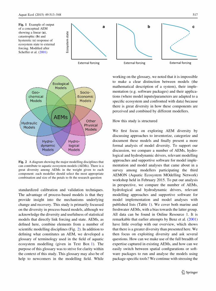
also qualifies as an AEM (Fig. 1). We exclude models
that focus on one single component of an ecosystem
(e.g. models that only deal with the population
dynamics of a given species), but include models that
zoom in on one part of the ecosystem (e.g. the fish or
macrophyte community) while treating the remainder
of the ecosystem in an aggregated way (typically
through the use of carrying capacities or mortality
rates). Two distinct classes of AEMs exist: those that
formulate a direct mathematical relation between
forcing and state (statistical models), and those that
are formulated in terms of the processes underlying
this relation (process-based models). Statistical mod-
els directly link forcing and state that can be derived
from data with standard statistical techniques. Linking
process-based models to data involves less
A. A. Van Dam
Department of Water Science and Engineering,
UNESCO-IHE Institute for Water Education,
PO Box 3015, 2601 DA Delft, The Netherlands
M. Weijerman
Joint Institute for Marine and Atmospheric Research
(JIMAR), University of Hawaii at Manoa, 1000 Pope
Road, Marine Science Bldg 312, Honolulu, HI 96822,
USA
S. A. Wells
Department of Civil and Environmental Engineering,
Portland State University, Portland, OR, USA
516 Aquat Ecol (2015) 49:513–548
123
standardized calibration and validation techniques.
The advantage of process-based models is that they
provide insight into the mechanisms underlying
change and recovery. This study is primarily focussed
on the diversity in process-based models, although we
acknowledge the diversity and usefulness of statistical
models that directly link forcing and state. AEMs, as
defined here, combine elements from a number of
scientific modelling disciplines (Fig. 2). In addition to
defining what constitutes an AEM, we developed a
glossary of terminology used in the field of aquatic
ecosystem modelling (given in Text Box 1). The
purpose of this glossary was to strive for clarity within
the context of this study. This glossary may also be of
help to newcomers in the modelling field. While
working on the glossary, we noted that it is impossible
to make a clear distinction between models (the
mathematical description of a system), their imple-
mentation (e.g. software packages) and their applica-
tions (where model inputs/parameters are adapted to a
specific ecosystem and confronted with data) because
there is great diversity in how these components are
perceived and combined by different modellers.
How this study is structured
We first focus on exploring AEM diversity by
discussing approaches to inventorize, categorize and
document these models and finally present a more
formal analysis of model diversity. To support our
discussion, we compare a number of AEMs, hydro-
logical and hydrodynamic drivers, relevant modelling
approaches and supportive software for model imple-
mentation and model analyses that came about in a
survey among modellers participating the third
AEMON (Aquatic Ecosystem MOdelling Network)
workshop held in February 2015. To put our analysis
in perspective, we compare the number of AEMs,
hydrological and hydrodynamic drivers, relevant
modelling approaches and supportive software for
model implementation and model analyses with
published lists (Table 1). We cover both marine and
freshwater AEMs, with a bias towards the latter group.
All data can be found in Online Resource 1. It is
remarkable that earlier attempts by Benz et al. (2001)
have little overlap with our overview, which shows
that there is a greater diversity than presented here.We
then focus on exploiting diversity and ask several
questions. How can we make use of the full breadth of
expertise captured in existing AEMs, and how can we
easily switch between spatial configurations or soft-
ware packages to run and analyse the models using
package-specific tools?We continue with stressing the
Ecos
yste
m st
ate
External forcing
a
External forcing
b
External forcing
cFig. 1 Example of output
of a conceptual AEM
showing a linear (a),catastrophic (b) andhysteretic (c) response ofecosystem state to external
forcing. Modified after
Scheffer et al. (2001)
Fig. 2 A diagram showing the major modelling disciplines that
can contribute to aquatic ecosystem models (AEMs). There is a
great diversity among AEMs in the weight given to each
component: each modeller should select the most appropriate
combination and size of the petals to fit the research question
Aquat Ecol (2015) 49:513–548 517
123
potential of ensemble modelling, and we end this
section with a discussion on how to exploit the full
range of approaches used in aquatic ecosystem
modelling. In the section on evolving diversity, we
describe the origins of the current diversity in AEMs
and discuss how model diversity could evolve in the
future and how standardization can facilitate this
process. In the final section, we discuss how we can
learn from concepts and techniques in biodiversity
research in our study on model diversity. Finally, we
provide a list of practical recommendations and a
perspective for the field of aquatic ecosystem mod-
elling in the next decade.
Exploring diversity in AEMs
AEMs have been and are being developed indepen-
dently in many places around the world. In this
section, we explore model diversity.
Making an inventory of the diversity in AEMs
An exploratory survey among 42 modellers partici-
pating in the third AEMONworkshop 2015 resulted in
133 different models, packages or programming
languages in use in the field of aquatic ecosystem
modelling (data presented in Online Resource 1,
Datasheet 2). We performed a Redundancy Analysis
(RDA, using the methods of Oksanen et al. 2014) on
39 AEMs from this list (results in Online Resource 2).
This analysis demonstrates that the professional
affiliation and country of origin played an important
role in determining knowledge and usage of models.
The driver behind this could be the research group’s
background, but also the diverging needs that moti-
vated the development of models, such as whether
there are mainly shallow lakes or deep reservoirs in a
specific country. Three approaches seem suited for
developing a more formal and ongoing inventory of
model diversity: (1) lists, (2) wikis and (3) code
repositories. We are not aware of an up-to-date list of
AEMs with a good coverage of the field. Laudable
attempts to list ecological models are UFIS (Knorren-
schild et al. 1996) and the ECOBAS initiative by
Joachim Benz (http://www.ecobas.org, Benz et al.
2001). ECOBAS provides metadata on a wide range of
models, including hydrological, hydrodynamic,
meteorological and ecological models. However, the
website has only rarely been updated since 2009;
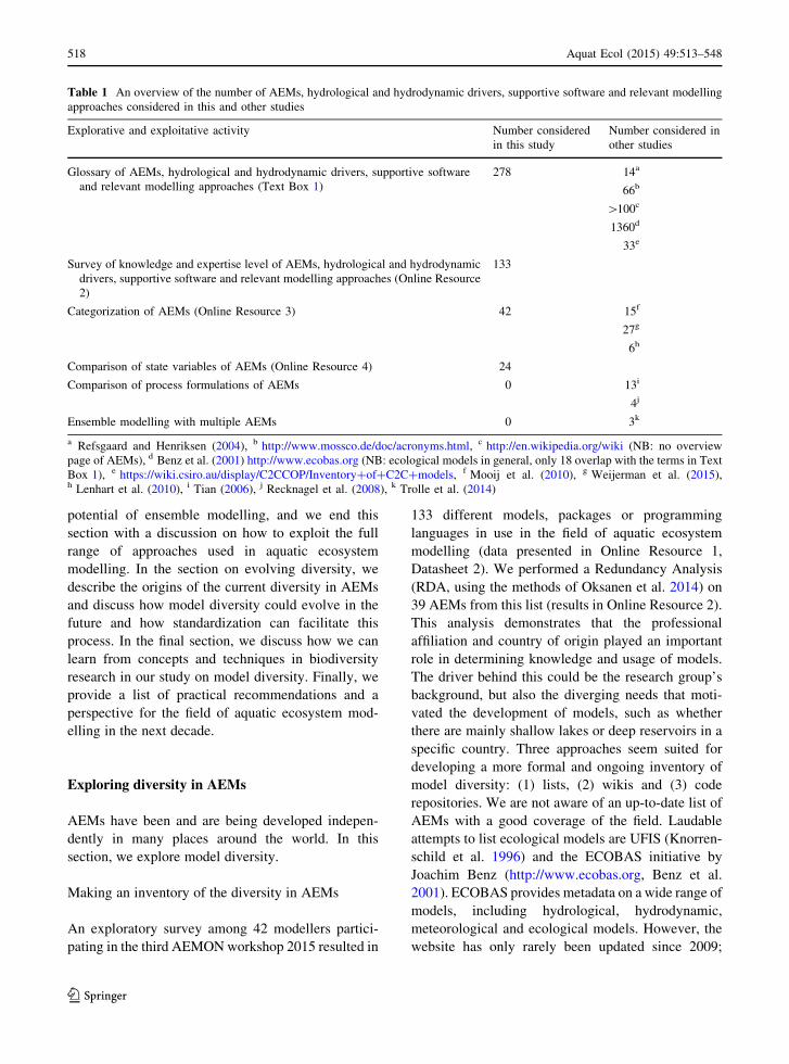
Table 1 An overview of the number of AEMs, hydrological and hydrodynamic drivers, supportive software and relevant modelling
approaches considered in this and other studies
Explorative and exploitative activity Number considered
in this study
Number considered in
other studies
Glossary of AEMs, hydrological and hydrodynamic drivers, supportive software
and relevant modelling approaches (Text Box 1)
278 14a
66b
[100c
1360d
33e
Survey of knowledge and expertise level of AEMs, hydrological and hydrodynamic
drivers, supportive software and relevant modelling approaches (Online Resource
2)
133
Categorization of AEMs (Online Resource 3) 42 15f
27g
6h
Comparison of state variables of AEMs (Online Resource 4) 24
Comparison of process formulations of AEMs 0 13i
4j
Ensemble modelling with multiple AEMs 0 3k
a Refsgaard and Henriksen (2004), b http://www.mossco.de/doc/acronyms.html, c http://en.wikipedia.org/wiki (NB: no overview
page of AEMs), d Benz et al. (2001) http://www.ecobas.org (NB: ecological models in general, only 18 overlap with the terms in Text
Box 1), e https://wiki.csiro.au/display/C2CCOP/Inventory?of?C2C?models, f Mooij et al. (2010), g Weijerman et al. (2015),h Lenhart et al. (2010), i Tian (2006), j Recknagel et al. (2008), k Trolle et al. (2014)
518 Aquat Ecol (2015) 49:513–548
123
updating is a challenge for any top-down initiatives.
An alternative could be an open community-based
approach, such as wikis, where multiple editors
independently contribute information. The obvious
and overwhelmingly successful example of this
approach is Wikipedia (http://www.wikipedia.org)
which maintains many lists, for instance of pro-
gramming languages (http://en.wikipedia.org/wiki/
List_of_programming_languages). The potential
lack of consistency of such community-based lists
seems to be compensated by the scope and imme-
diacy of the information provided and the commit-
ment resulting from the community-based approach.
The third option is code repositories, such as
SourceForge (http://sf.net) and GitHub (http://
github.com), which are increasingly popular plat-
forms enabling open-source communities to develop
software and distribute code.
Documenting diversity in AEMs
To preserve and communicate model diversity,
proper documentation of models is crucial. There
is no standard way of documenting AEMs, and
different model developers have different methods
to obtain and save their information. The existing
ODD protocol (overview, design concepts and
details) for individual-based models (Grimm et al.
2006), the Earth System documentation project
(http://es-doc.org) or the TRACE approach
(TRAnsparent and Comprehensive Ecological mod-
elling documentation) might be adopted by aquatic
ecosystem modellers in the future (Grimm et al.
2014). Models can be documented through model
homepages, scientific publications or grey literature
reports. Wikipedia is not an option because it has a
strict policy of not being a primary source of doc-
umentation but instead only providing referenced
information. To be useful in the current practice of
scientific research, any type of documentation
should be accessible through the Internet, preferably
with open access. The majority (71 %) of the AEMs
analysed in Online Resource 3 has a website that
provides model documentation. Furthermore, for
86 % of the models, we could identify a primary
publication; however, only three out of 42 AEMs
analysed in Online Resource 3 have a page on
Wikipedia (Ecopath, PCLake and PCDitch).
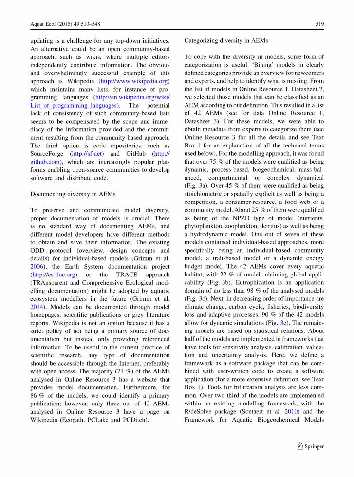
Categorizing diversity in AEMs
To cope with the diversity in models, some form of
categorization is useful. ‘Bining’ models in clearly
defined categories provide an overview for newcomers
and experts, and help to identify what is missing. From
the list of models in Online Resource 1, Datasheet 2,
we selected those models that can be classified as an
AEM according to our definition. This resulted in a list
of 42 AEMs (see for data Online Resource 1,
Datasheet 3). For these models, we were able to
obtain metadata from experts to categorize them (see
Online Resource 3 for all the details and see Text
Box 1 for an explanation of all the technical terms
used below). For the modelling approach, it was found
that over 75 % of the models were qualified as being
dynamic, process-based, biogeochemical, mass-bal-
anced, compartmental or complex dynamical
(Fig. 3a). Over 45 % of them were qualified as being
stoichiometric or spatially explicit as well as being a
competition, a consumer-resource, a food web or a
community model. About 25 % of themwere qualified
as being of the NPZD type of model (nutrients,
phytoplankton, zooplankton, detritus) as well as being
a hydrodynamic model. One out of seven of these
models contained individual-based approaches, more
specifically being an individual-based community
model, a trait-based model or a dynamic energy
budget model. The 42 AEMs cover every aquatic
habitat, with 22 % of models claiming global appli-
cability (Fig. 3b). Eutrophication is an application
domain of no less than 98 % of the analysed models
(Fig. 3c). Next, in decreasing order of importance are
climate change, carbon cycle, fisheries, biodiversity
loss and adaptive processes. 90 % of the 42 models
allow for dynamic simulations (Fig. 3e). The remain-
ing models are based on statistical relations. About
half of the models are implemented in frameworks that
have tools for sensitivity analysis, calibration, valida-
tion and uncertainty analysis. Here, we define a
framework as a software package that can be com-
bined with user-written code to create a software
application (for a more extensive definition, see Text
Box 1). Tools for bifurcation analysis are less com-
mon. Over two-third of the models are implemented
within an existing modelling framework, with the
R/deSolve package (Soetaert et al. 2010) and the
Framework for Aquatic Biogeochemical Models
Aquat Ecol (2015) 49:513–548 519
123
(FABM) (Bruggeman and Bolding 2014) being the
most used of the 12 modelling frameworks that we
encountered (Fig. 3d). One can rightfully say that the
field of aquatic ecosystem modelling is quite scattered
when it comes to the use of modelling frameworks.
This notion was one of the incentives for developing
Delft3D-Delwaq (Deltares 2014), FABM (Bruggeman
and Bolding 2014) and the Database Approach to
Modelling (DATM) (Mooij et al. 2014). With 50 %,
FORTRAN is the dominant programming language
for coding AEMs (Fig. 3f). Next comes C or C??
(together 26 %), Delphi (15 %) and R (15 %). The
majority of AEMs are implemented as ordinary or
partial differential equations (Fig. 3g).
100%
Sim. temporaldynamics
Scenarioanalysis
Sensi�vityanalysis
Calibra�onValida�on
Uncertaintyanalysis
Bifurca�onanalysis
e
0%20%40%60%80%
100%Eutrophica�on
Climate change
Carbon cycle
Fisheries
Biodiversityloss
Adap�veprocesses
c
0%
20%
40%
60%
80%
100%Shallow lakes
Reservoirs
Deep lakes
Rivers
Estuaries
Seas
Ditches/canals
Oceans
Wetlands
Catchments
Global
Coastalb
0%10%20%30%40%50%
Par�al diff. eq.
Ordinary diff.eq.
Differenceequa�ons
Input-outputrela�on
Agent-basedevent driven
La�ce diff. eq.
g
0%
20%
40%
60%
80%
100%Aqua�c Ecosystem model
Dynamical modelProcess-based model
Biogeochemical model
Mass balanced model
Compartment model
Complex dynamical model
Stoichiometric modelSpa�ally explicit model
Compe��on modelConsumer-resource model
Foodweb model
Community model
NPZD model
Hydrodynamical model
Individual-based model
Trait-based modelDEB model
a
0%
5%
10%
15%
20%R/deSolve
FABM
Web Tool
DELWAQ
DUFLOW
Matlab
AQUASIM
Ecopath
Stella
ACSL
GRIND
OSIRISd
0%10%20%30%40%50%FORTRAN
C
Delphi
R
C++
MatlabPython
Visual Basic
DUPROL
Through GUI
JAVA
ACSL
f
Fig. 3 Outcome of a
categorization of 42 AEMs
on six types of
categorizations: a modelling
approach (for all levels, see
Online Resource 2),
b environmental domain of
the model, c model
application domain,
d modelling framework,
e type of analysis available
within the model’s
framework, f programming
language and
g mathematical equation
type. See text for
explanation
520 Aquat Ecol (2015) 49:513–548
123
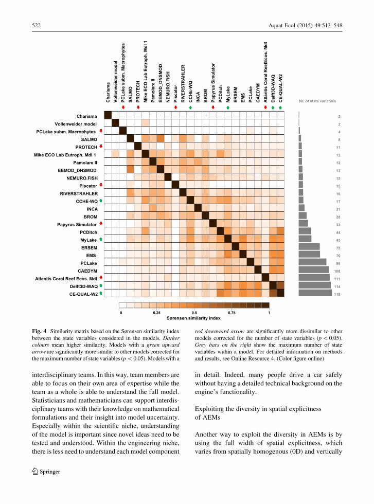
Analysing diversity in AEMs
Analysing model diversity goes beyond the more
descriptive approach mentioned above. Here, the aim
was to identify whether we are dealing with true
diversity or ‘pseudo-diversity’. Models are often
related to each other. The MyLake model (Saloranta
and Andersen 2007), for example, has characteristics
that are also found in other lake models such as
DYRESM-CAEDYM (Hamilton and Schladow
1997), MINLAKE (Riley and Stefan 1988), PROBE
(Blenckner et al. 2002) and BELAMO (Omlin et al.
2001; Mieleitner and Reichert 2006). We aim for a
more objective and in-depth analysis of a list of AEMs
using a similarity index (for details on the analysis, see
Online Resource 4 and for the data Online Resource 1,
Datasheet 4). One approach is to compare state
variables between models. We analysed 24 AEMs
for which sufficient information was provided, which
gave in total almost 550 unique state variables. The
minimum number of state variables found in a model
is 2 and the maximum is 118 (Fig. 4). It should be
noted that in some (especially the larger and general)
models, not all state variables are included simultane-
ously in each model application but rather subsets of
variables are being used. Additionally, some models
have state variables that can be duplicated by changing
their parameters (e.g. cohorts of a species). A Sørensen
similarity analysis (Sørensen 1948) using the state
variables of 24 models (Online Resource 4) shows that
models become more similar as their complexity
increases. This is an expected result as the chance of
similarities increases with increasing sampling size of
a given pool. However, overall the dissimilarity is
higher than the similarity since more than 80 % of the
models have a similarity index of less than 0.25.
Hence, many models benefit from predecessor models
even though they are still unique with individual
features not found in predecessor models. Most
overlap can be found in general state variables such
as phosphorus, ammonia and a generic group of
phytoplankton or zooplankton. Three groups of mod-
els can be distinguished: general-purpose models with
a relative high overlap, specialized models with low
overlap and intermediate models with an intermediate
level of overlap (see dendrogram in Online Resource
4). Interestingly, some models are significantly more
dissimilar than would be statistically expected based
on their number of state variables (red downward
arrow, Fig. 4). This is because these models capture
only a specific non-overlapping part of the aquatic
ecosystem (e.g. the Guam Atlantis Coral Reef Ecosys-
tem Model versus PCLake or CAEDYM). Other
models are more similar than would be expected based
on the number of state variables (upward green arrow);
these models simulate the aquatic ecosystem in a more
general way, such as CCHE and Mylake. A following
step could be to compare the models for their
mathematical process formulations, though this is
beyond the scope of this paper. An educated guess is
that this will reveal an even higher diversity, as endless
combinations can be made with the available process
formulations. For example, Tian (2006) counted 13
functions used to describe the effect of light forcing on
phytoplankton growth. Using these light functions in
combination with other functional relations, for
instance, temperature forcing (10 different relations),
zooplankton feeding (20 different relations), prey
feeding (15 different relations) and mortality (8
different relations), lead to hundreds of thousands of
combinations that give different results and are all ‘the
best’, depending on the aim of the model (Gao et al.
2000).
Exploiting diversity in AEMs
The inventory of the AEMs reveals a great diversity in
model approaches, formulations and applications.
Here, we ask whether and how this diversity could
be exploited.
Exploiting the diversity in disciplines
One of the options is to exploit the diversity in
contributing disciplines (see Fig. 2) and work in teams
consisting of not only aquatic ecologists, but also
social scientists, economists, climatologists, hydrolo-
gists, statisticians, mathematicians, etc. Working in an
interdisciplinary setting helps one to look beyond the
personal expert field and provides a more holistic view
upon both models and aquatic ecosystems (Hamilton
et al. 2015). Resulting interdisciplinary models have
an increased complexity with the disadvantage that
full understanding of the model by the individual
modeller is lost (Scholten et al. 2007; Robson 2014a).
The problem of inappropriate usage of complex
models can be overcome by again working in
Aquat Ecol (2015) 49:513–548 521
123
interdisciplinary teams. In this way, teammembers are
able to focus on their own area of expertise while the
team as a whole is able to understand the full model.
Statisticians and mathematicians can support interdis-
ciplinary teams with their knowledge on mathematical
formulations and their insight into model uncertainty.
Especially within the scientific niche, understanding
of the model is important since novel ideas need to be
tested and understood. Within the engineering niche,
there is less need to understand each model component
in detail. Indeed, many people drive a car safely
without having a detailed technical background on the
engine’s functionality.
Exploiting the diversity in spatial explicitness
of AEMs
Another way to exploit the diversity in AEMs is by
using the full width of spatial explicitness, which
varies from spatially homogenous (0D) and vertically
Cha
rism
aVo
llenw
eide
r mod
elPC
Lake
sub
m. M
acro
phyt
esSA
LMO
PRO
TEC
HM
ike
ECO
Lab
Eut
roph
. Mdl
1Pa
mol
are
IIEE
MO
D_D
NSM
OD
NEM
UR
O.F
ISH
Pisc
ator
RIV
ERST
RA
HLE
RC
CH
E-W
QIN
CA
BR
OM
Papy
rus
Sim
ulat
orPC
Ditc
hM
yLak
eER
SEM
EMS
PCLa
keC
AED
YMA
tlant
is C
oral
Ree
fEco
s. M
dlD
elft3
D-W
AQ
CE-
QU
AL-
W2
Nr. of state variables
Charisma 2
Vollenweider model 2
PCLake subm. Macrophytes 4
SALMO 8
PROTECH 11
Mike ECO Lab Eutroph. Mdl 1 12
Pamolare II 12
EEMOD_DNSMOD 13
NEMURO.FISH 15
Piscator 15
RIVERSTRAHLER 16
CCHE-WQ 17
INCA 21
BROM 28
Papyrus Simulator 33
PCDitch 44
MyLake 45
ERSEM 75
EMS 76
PCLake 98
CAEDYM 108
Atlantis Coral Reef Ecos. Mdl 111
Delft3D-WAQ 114
CE-QUAL-W2 118
0 0.25 0.5 0.75Sørensen similarity index
1
Fig. 4 Similarity matrix based on the Sørensen similarity index
between the state variables considered in the models. Darker
colours mean higher similarity. Models with a green upward
arrow are significantly more similar to other models corrected for
themaximumnumber of state variables (p\ 0.05).Models with a
red downward arrow are significantly more dissimilar to other
models corrected for the number of state variables (p\ 0.05).
Grey bars on the right show the maximum number of state
variables within a model. For detailed information on methods
and results, see Online Resource 4. (Color figure online)
522 Aquat Ecol (2015) 49:513–548
123
or horizontally structured (1D) to fully 3D. Within
these dimensions, a modeller can additionally
choose between different structured grids (e.g.
Cartesian grid, regular grid and curvilinear grid)
and unstructured grids (e.g. finite elements). Fol-
lowing Occam’s razor, model complexity should be
minimized and only increased if this increases the
predictive performance of the model or its general-
ity/universality (please note that, while mentioned
here in the context of spatial explicitness, Occam’s
razor applies to all aspects of complexity in AEMs).
Therefore, to understand the basics of ecological
processes in a well-mixed system, one should use a
0D model as its dynamics are often easier to
understand. Additionally, 0D models are well suited
for checking the internal consistency of the model
functions. Spatially explicit models, however, are
more realistic, as they account for the spatial
heterogeneity of ecosystems, with the risk of getting
lost in complexity when explaining model beha-
viour. Nonetheless, some research questions cannot
be solved without taking spatial resolution into
account [e.g. population dynamics of fish in Jackson
et al. (2001), and spatial distribution of macrophytes
and algae in Janssen et al. (2014)]. Recent advances
facilitate the implementation of a model in different
spatial settings. For example, with Delft3D-Delwaq,
FABM and DATM, it is possible to switch between
a 0D, 1D, 2D to 3D implementation of, for instance,
PCLake (Van Gerven et al. 2015). However, these
frameworks are currently implemented without
accounting for feedbacks between ecology and
hydrodynamics. Interfaces such as OpenMI (Gre-
gersen et al. 2007) and FABM (Bruggeman and
Bolding 2014) allow for such coupling and are
designed to overcome the issues that emerge when
integrating ecology and hydrodynamics. Examples
of these issues are the different timescales and
spatial schematization for ecology and hydrodynam-
ics (e.g. Sachse et al. 2014) and feedbacks between
ecology and hydrodynamics, such as the effects of
water plants on the water flow (e.g. Berger and
Wells 2008).
Exploiting diversity by having a given AEM
implemented in multiple frameworks
Recent approaches such as DATM (Mooij et al. 2014),
FABM (Bruggeman and Bolding 2014) and the open
process library in Delft3D-Delwaq (Deltares 2014)
make it possible to exploit model implementations in
multiple frameworks without much overhead. There-
fore, a myriad of tools for model analysis (e.g.
sensitivity analysis, calibration, validation, uncer-
tainty analysis, and bifurcation analysis) become
easily available. The redundancy in tools among
frameworks insists modellers to stick to the framework
they are familiar with for most analyses, whereas the
complementarity in tools is tempting to switch to other
frameworks for alternative analyses (Van Gerven et al.
2015), including the switch between 0D and 3D. In
this way, the strengths of frameworks (including run-
time) can be exploited, and the underlying ecological
question can be approached from different
perspectives.
Exploiting diversity in dealing with uncertainty
in AEMs
As a simplification of nature, AEMs suffer from
uncertainty in their outcomes (Beck 1987; Chatfield
1995; Draper 1995). Sources of uncertainty are
structural uncertainties, i.e. incomplete or imperfect
process formulations, parameter uncertainty, uncer-
tainty in forcing functions and initial values, uncer-
tainty in validation data, and uncertainty due to the
numerical methods used. A full coverage of the topic
of uncertainty in AEMs is beyond the scope of this
paper. For more information on this topic, we refer to
the extensive literature available on this topic includ-
ing Beck (1987), Chatfield (2006) and Doherty (2015).
Below, we limit ourselves to presenting three different
views on how to deal with uncertainty in parameters.
First, a modeller measures the parameters’ magnitudes
directly. The parameter values are then purely based
on biologically, chemically or physically knowledge.
Due to errors in the measurements (experimental
uncertainty, Moffat 1988) and limited transferability
(e.g. between laboratory and field conditions), these a
priori parameter values have an uncertainty as well
(Draper 1995). By repeating the measurements over
and over, the experimental uncertainty can be reduced,
thereby minimizing the parameter uncertainty, but this
is often a costly measure (Chatfield 1995). A second
option is to estimate the parameters using calibration
data and statistics without the use of a priori knowl-
edge. This method leads in many cases to multiple
possible parameterizations of the model with equal fit
Aquat Ecol (2015) 49:513–548 523
123
(e.g. Beven 2006) and bears the risk of overfitting
(Hawkins 2004). For this reason, a modeller may
choose for the third option where the parameters are
estimated based on calibration data, statistics and a
priori knowledge (e.g. Janse et al. 2010). In this case, a
realistic range of parameter values is defined, prior to
the parameter estimation by statistics. Thereafter,
using Bayesian statistics, the parameters can be
estimated within the range of realism (Gelman et al.
2014).
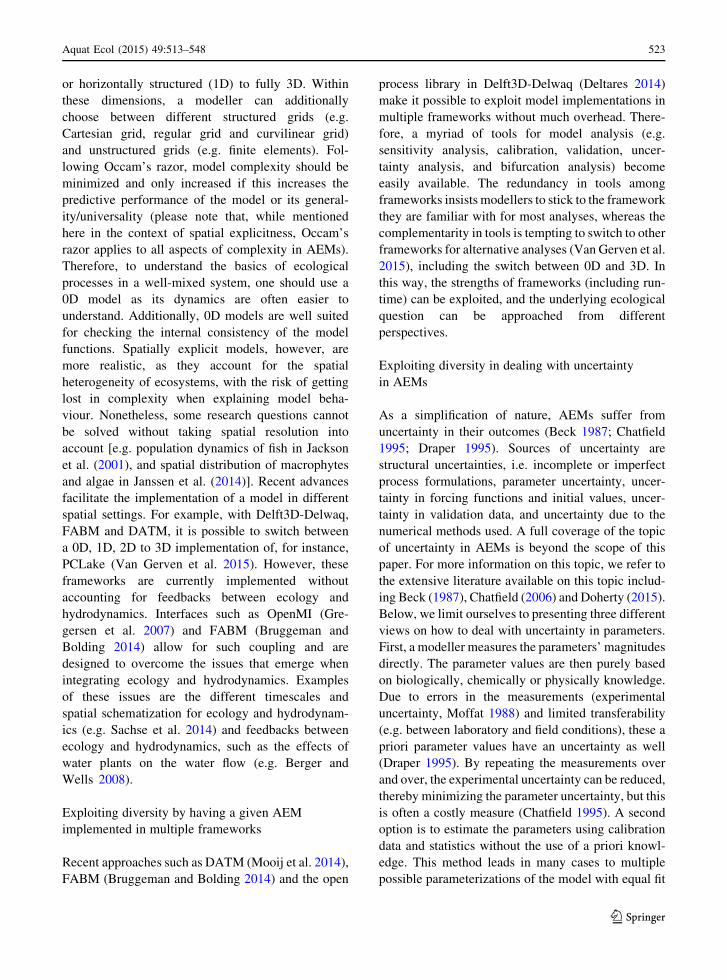
Exploiting diversity by ensemble modelling
with AEMs
One way to deal with the uncertainty is using the
diversity of models in ensemble techniques [e.g.
Ramin et al. (2012) or Trolle et al. (2014), see Fig. 5
for an example from the latter study]. A variety of
ensemble techniques exists, each duplicating a certain
aspect of the modelling process. In multi-model
ensembles (MMEs), multiple models are applied to a
given problem. Single-model ensembles use different
model inputs (parameters, initial values, boundary
conditions) to exploit the model’s sensitivity (e.g.
Couture et al. 2014; Gal et al. 2014 or Nielsen et al.
2014). More ensemble techniques or combinations of
techniques exist including multi-scheme ensembling
(use of different numerical schemes) and hyper-
ensembling (use of multiple physical processes).
Ensemble modelling has become a standard in
meteorological forecasting (e.g. Molteni et al. 1996)
and climatic forecasting (e.g. IPCC 2014). There is an
increasing number of applications in hydrology and
hydrodynamics as well (e.g. Stepanenko et al. 2014;
Thiery et al. 2014). In aquatic ecosystem modelling,
the use of ensemble techniques is still rare (but see
examples in, for instance, Lenhart et al. 2010; Ramin
et al. 2012; Gal et al. 2014; Nielsen et al. 2014; Trolle
et al. 2014). However, the relevance of MME for
ecological modelling is large, as a strictly physically
based description is not practically feasible and a
unified, transferable set of equations is, therefore, not
available. Additionally, we foresee that ensemble
modelling will become common practice because of
(1) the emergence of active communities of aquatic
ecosystem modellers such as AEMON; (2) the
increase in freely available papers, data and model
code; and (3) the development of approaches such as
Delft3D-Delwaq, FABM and DATM. Hence, the
results of decades of individual model niche develop-
ment can now be better utilized (Mooij et al. 2010;
Trolle et al. 2012). The comparative list provided in
Online Resource 1 (Datasheet 4) is a useful starting
point of ensemble modelling with AEMs. When using
a model to provide forecasts, MME have two major
advantages over single-model approaches. First, the
ensemble mean may be a better predictor than any of
the sole ensemble members (Trolle et al. 2014). This is
especially true when an aggregated performance
measure over many diagnostics variables is considered
Fig. 5 Example of a multi-model ensemble (MME). The
shaded area shows the full width of predicting outcomes made
by different models, the black line shows the mean of all models
and the circles are the observations. Figure modified after Trolle
et al. (2014) where the authors show that the prediction by the
average model outcome is better than the prediction by
individual models
524 Aquat Ecol (2015) 49:513–548
123
(Hagedorn et al. 2005; Trolle et al. 2014). Second, the
ensemble spread can serve as a convenient measure of
predictive uncertainty if a spread–skill correlation
exists. AlthoughMMEs are attractive, their limitations
need to be recognized. First, despite ever increasing
computer power, they are time-consuming to put in
place. More importantly, MME-based estimates of
structural uncertainty can only be meaningful if the
models involved differ substantially. Another more
general limitation of ensembles is that the attainable
estimate of uncertainty is inevitably incomplete, for
example due to a limited number of suitable models
and the requirement of each model to have its own set
of—ideally standardized—parameters and initial val-
ues. Ensemble techniques therefore only quantify part
of the total uncertainty in predictions (Krzysztofowicz
1999). In the context of ecological process-based
modelling though, the integration of multiple models
should not be viewed solely as an approach to improve
our predictive devices, but also as an opportunity to
compare alternative ecological structures, to challenge
existing ecosystem conceptualizations, and to inte-
grate across different (and often conflicting) para-
digms (Ramin et al. 2012). Future research should also
focus on the refinement of the weighting schemes and
other performance standards to impartially synthesize
the predictions of different models. Several interesting
statistical post-processing methods presented in the
field of ensemble weather forecasting will greatly
benefit our attempts to develop weighting schemes
suitable for the synthesis of multiple ecosystem
models (Wilks 2002). Other outstanding challenges
involve the development of ground rules for the
features of the calibration and validation domain, the
inclusion of penalties for model complexity that will
allow building forecasts upon parsimonious models,
and performance assessment that does not exclusively
consider model endpoints but also examines the
plausibility of the underlying ecosystem structures,
i.e. biological rates, ecological processes or derived
quantities (Arhonditsis and Brett 2004).
Exploiting the diversity in fundamentally different
approaches in aquatic ecosystem modelling
Finally, we could exploit the diversity in more
fundamentally different model approaches, for exam-
ple statistical- versus process-based models. The
diversity in model approaches is the product of the
numerous choices that can be made during model
development, pursuing a certain trade-off between
effort, model simplicity, realism, process details,
boundary conditions, forcings and accuracy along
various dimensions such as time and space (e.g.
Weijerman et al. 2015). For example, minimal models
aim to understand the response curve of ecosystems to
disturbances, but they are generally too simple to
allow for upscaling and process quantification. Com-
plex models on the other hand can describe the cycling
of nutrients through many compartments of an
ecosystem as well as the flow of energy through the
system. Therefore, they often allow for quantitative
scenario evaluations, but their output is difficult to
interpret as it is demanding to decipher the numerous
interactions and feedback loops. More complexity also
can be introduced by individual-based and trait-based
models, which allow the inclusion of evolutionary
processes. Thus, a higher diversity of model
approaches permits addressing a higher number of
different purposes, provided that they are sufficiently
complementary. There is a great value in combining
different modelling approaches, as insights gained by
one model can be useful for the application of another,
and we benefit from the strengths of different model
types (Mooij et al. 2009). Combining modelling
approaches helps to develop an integrative view on
the functioning of aquatic systems and seems almost
essential for the adaptive management of the source
and sink functions of lake ecosystems, which require
integrated thinking and decision support.
Evolving diversity in AEMs
We have explored and exploited diversity in AEMs.
Before reflecting on possible future evolution of
model diversity, it is interesting first to look back
and see how the existing diversity came about.
A historical perspective on evolving diversity
in AEMs
The field of AEMs started with great expectations
when the first mainframe computers were installed at
universities in the 1960s (Lavington 1975). But
because of the adaptive nature of living systems,
making predictive AEMs proved to be more difficult
than predicting the trajectory of a rocket to the moon.
Aquat Ecol (2015) 49:513–548 525
123

This sparked the emergence of individual-based
models sensu lato, including dynamic energy budget
models (Kooijman 1993), structured population mod-
els (De Roos et al. 1992) and individual-based models
sensu stricto (Mooij and Boersma 1996), that zoom in
on a particular (group of) species in the ecosystem. In
an opposite direction, minimal dynamical models of
ecosystems zoomed out to detect dominant nonlinear-
ities in ecosystem responses to external forcing
(Scheffer et al. 2001). Renewed interest in large
ecosystem models occurred in the past decades, not
the least as a result of the increased and distributed
computational power, but this time with the tendency
to link the models with individual-based and trait-
based approaches (DeAngelis and Mooij 2005) and
compare their behaviour with minimal dynamical
models (Mooij et al. 2009). In the past, region-specific
questions have led to region-specific models; how-
ever, as a result of current globalization, the need for
widely applicable models and models covering
regional or continental aspects is rapidly increasing.
The growing recognition of the importance anthro-
pogenic stressors on ecosystems and the services
provided by ecosystems asks for coupling of ecolog-
ical models with socio-economics models (e.g. Down-
ing et al. 2014). This can be realized by using output of
one model as input for the other model, or run-time
exchange of input and output between such models.
The latter method is more complicated and only
becomes necessary when there are strong feedbacks
between ecology and socio-economics.
Arguments for reducing diversity
There are valid arguments why aquatic ecology as a
whole could benefit from streamlining the diversity in
AEMs. First, some formulations have been shown to be
both less accurate and more complex than alternatives
(Tian 2006). Second, some models are developed to
answer one specific question and thus lose their
functionality once this question has been addressed. It
is likely that this kind of models has a high turnover
rate, but suchmodels could also be incorporated in large
models as the results prove to be relevant. Finally, the
presence of pseudo-diversity is an argument to reduce
the number of models. For example, in climate studies,
it has been shown that the performance of ensemble
models significantly improved when pseudo-diversity
was reduced (Knutti et al. 2013). Ideally, groups that
work in parallel on similar models should have the
incentives to join efforts, but these incentives are often
not in place. Also at the level of the individual
scientists, there seem to be few, if any, incentives to
give up one’s own model, whereas there are many
incentives to maintain it or even start yet another one.
Only when the incentives that lead to fragmentation are
overcome, or are outweighed by incentives to join
forces, can we expect a healthy consolidation of the
field to take place. Frameworks such as Delft3D-
Delwaq (Deltares 2014), FABM (Bruggeman and
Bolding 2014) and DATM (Mooij et al. 2014) facilitate
this process, but also these frameworks have the risk to
be duplicated, leading to yet another layer of fragmen-
tation. The turnover rate of AEMs is hard to measure
since publications on dropped models are rare, if they
even exist. At the same time, the absence of publica-
tions on a specific model does not necessarily mean that
a model became unused, as engineers, for example,
might use the specific model on a daily basis without
publishing the results. Furthermore, unlike extinct
species that reduce biodiversity, ‘dead’ models can
become ‘alive’ when a need for their existence emerges,
thereby contributing again to model diversity.
Arguments for enlarging diversity
Because the field of aquatic ecosystem modelling can
appear quite fragmented, arguments for enlarging
diversity in AEMs are easily overlooked. Neverthe-
less, there should always be room for good ideas and
new avenues. An interesting example is provided by
minimal dynamical models. When these became
prominent in the shallow lake literature about 25 years
ago, they were met with considerable reservation and
hardly perceived as a step forward. Nowadays, their
ability to illustrate and communicate essential nonlin-
earity in the response of ecosystem (and many other
dynamical systems) is broadly recognized (Scheffer
et al. 2001). Another emerging approach with many
applications in the aquatic domain is Dynamic Energy
Budgets (DEB) (Kooijman 1993). The scope of
current DEB models, however, is too limited to be
qualified as ecosystem models as defined in this study.
Arguments for conserving diversity
With the first generation of aquatic ecosystem mod-
ellers about to retire, there can be serious concern about
526 Aquat Ecol (2015) 49:513–548
123
a loss of useful models and approaches, requiring active
conservation effort by the community at large. Proper
implementation of conservation schemes will help to
prevent the proverbial ‘reinvention of the wheel’
(Mooij et al. 2010). Additionally, it can help future
model developers to anticipate what models and
formulations worked well and which did not. Obvi-
ously, this learning process is hampered at the lack of
documentation of failures in the scientific literature.
Conserving diversity would thus have a great educa-
tional value and would help understand the ‘genealogy’
of the existing models. Conservation of model diversity
is important for science as well, as science builds on
repetition which only can be complied with when code
is conserved. However, model diversity conservation
has to overcome ‘code rot’, which is the deterioration of
software as a result of the ever evolving modelling
environment, making the software invalid or unusable
(Scherlis 1996). To prevent code rot, the code should be
maintained. Another option is to conserve models in
their purest mathematical form (e.g. like in the concept
behind DATM, Mooij et al. 2010).
How to facilitate evolving diversity
One would like to have tools available and mechanisms
in place that would allow diversity to evolve through a
‘natural selection’ of models. Natural selection is an
emergent property of a system in which there is
variation among agents; this variation is transferred to
the offspring of the agents and has an impact on the
survival of the agents. We have shown that there is
ample diversity among AEMs, and there seems to be a
healthy cross-fertilization of ideas leading to continued
development of new versions andmodels.What may be
hampering ‘natural selection’ among AEMs, however,
are standardized methods to compare model ‘fitness’
within their niche and given the research question they
address. Here, we point specifically to the research
question since models might have a different purpose,
and it only makes sense to compare the fitness of those
models that are able to answer the same research
question. To enhance selection and ‘gene transfer’, easy
model accessibility is necessary in the first place. Easy
accessibility not only includes freely available model
software but also low time costs of, for instance,
learning new modelling code or approaches. Addition-
ally, data availability is very important for the improve-
ment of models (Hipsey et al. 2015). As long as models
are inaccessible, due to, for example, licence restric-
tions or inappropriate manuals, modellers will most
likely choose the models in use by their colleagues (see
Online Resource 2). These easily accessible models
may not be the best suitable to answer their questions.
Secondly, standard objective assessment criteria to
calibrate and validate models are important (Refsgaard
et al. 2005; Robson 2014b). These criteria are different
for each modelling niche, as models that are suitable,
for example, for forecasting of algal blooms require
other criteria than models suitable for biodiversity
assessments. It also implies providing a freely acces-
sible set of data used as calibration or validation data
(meteorology, hydrology, hydrodynamics, nutrient
fluxes, etc.) of the models to be benchmarked. The
application of the models to these common test data
enables a direct comparison without interfering effects
from differences in basin morphometry, hydrology,
meteorology, and so on. The main idea behind this
benchmarking is not to classify models into ‘good’ and
‘bad’ ones, but instead to characterize the dynamic
behaviour and specific abilities of the separate models.
Finally, we would like to point to the importance of the
conservation and maintenance of expertise and expe-
rience for model evolution. Currently, project life
cycles are generally short, and while mobility of people
can help to spreadmodels, the samemobility could lead
to a local loss of expertise (Herrera et al. 2010; Parise
et al. 2012).
Discussion
How can biodiversity research help us to interpret
model diversity?
One could see the myriad of model purposes as niches
that shape model diversity. Like biodiversity, model
diversity can be organized in taxonomic structures to
classify models. Using Wikipedia as a reference, such a
taxonomic studyhas beendone already forprogramming
languages and showed a phylogenetic tree with new
programming languages emerging from different ele-
ments of earlier programming languages (Valverde and
Sole 2015).A similar study forAEMs is intriguing, but is
beyond this study.Our analysis revealed a large diversity
in themodels.Weargue that to fully exploit the niche, the
tools for analysis provided in eachmodelling framework
should be used. If we divide the AEMs in specialists or
Aquat Ecol (2015) 49:513–548 527
123
generalists, the majority of the AEMs seem to be
specialists that address the research question that led to
their development but with little application beyond.
This can be attributed to the fact that models are often
locked within frameworks which obstruct communica-
tion and cross-fertilization between the models (Mooij
et al. 2014). For the same reason, we could question
whether there is enough competitionbetween themodels
to enable survival of the fittest and thus competitive
exclusion. At present, most models seem to have the
fingerprints of the resource group it is developed in, as if
they were species that evolved in their island-specific
supported niche. This has the disadvantage of reinvent-
ing the wheel, but surely has its advantage as well since
the independently evolved models can be used for
comparison as in ensemble modelling.
Recommendations
Our analysis of exploring, exploiting and evolving
diversity in AEMs leads us to three types of recom-
mendations related to (1) availability, (2) standard-
ization and (3) coupling of AEMs.
Availability of AEMs
With respect to the availability of AEMs, it is important
to continue the current trend of open-source policies for
AEM models, tools for analysis and data. This will
increase the transparency of model structure, assump-
tions and approaches. Besides that, there is an urgent
need for a public overview of existing AEMs. This
could be aWikipedia list, with links to relevant (online)
documentation or similar initiatives. Such a list could
be complemented with an overview of the forces and
niches that created the existing diversity in AEMs.
Once there is an overview of the niches inwhichmodels
are designed, the suitability of models for other
applications is better assessed. Documentation of the
available AEMs will create awareness of the full width
of approaches in AEMs to avoid tunnel vision. We
should also actively preserve AEMs to learn from the
past and thereby avoid reinventing the wheel but also to
identify and prevent pseudo-diversity in AEMs.
Standardization of AEM practices
We recommend developing standardization in the
documentation of AEMs [comparable with, e.g. ODD
for IBMs, Grimm et al. (2006)], terminology to
categorize AEMs and the methods to analyse AEMs.
Standardization of documentation and terminology is
desirable for the communication on the different
available models. Standardization of methods for
parametrization, comparison, calibration, testing,
structuring, conversion and interpolation in AEMs
will lead to a common practice in model analysis.
Linking AEMs
In our analysis, we compared models by their state
variables, while additional diversity is hidden in the
process formulations. Here, we recommend fulfilling
the next step by comparing models by their process
formulations. Currently, this step is a time-consuming
and difficult task as a result of lack in the availability
of model definitions. Perhaps this step will be possible
in the future due to the emerging linking approaches
such as DATM. And linking has more benefits. We
advocate linking AEMs with models from other
disciplines to answer questions that require a holistic
approach. We recommend running AEMs in more
than one spatial setting to gain more insight into the
effects within the spatial context and suggest running a
given AEM in multiple frameworks to use the full set
of tools for analysis and advice of the user community.
Finally, we recommend ensemble modelling with
AEMs in order to use the best out of multiple models.
For example, statistical- and process-based AEMs
should be used side by side because they have
complementary strengths.
We anticipate that increasing model availability,
standardization of model documentation, and various
forms of linking will lead to an evolving diversity of
AEMs in which the better performing models out-
compete the poorer performing models. Given the
large number of model niches, however, there will
always remain a great diversity in AEMs.
Perspectives
We can only speculate where the field of aquatic
ecosystem modelling will be heading in the coming
five to 10 years. We expect that many new develop-
ments will be triggered and enabled by general trends
in science, technology and society. Here, we list 10 of
these possible trends. (1) We expect that wikis (e.g.
Wikipedia), where users can either retrieve information
528 Aquat Ecol (2015) 49:513–548
123
or contribute information through standardized web
interfaces, will gain in importance for the documenta-
tion and distribution of AEMs. While we recognize the
inherent lack of quality control, we highly value the
ease of access, the community effort and dynamic
nature of this approach (the name ‘wiki’ is derived from
the Hawaiian word for ‘quick’). (2) We recognize
initiatives to develop e-infrastructures for the imple-
mentation of AEMs and other environmental models
where users of different levels of experience share easy
and secure access to models and data according to their
needs. (3) We envision that current trends in the
mandatory storage of scientific data in repositories will
be extended to model code. (4) We envision that online
databases of model parameters will be developed and
become an important resource for the development and
improvement of AEMs. (5) We see a change from the
way consultancy companies earn money with AEMs.
Formerly, their businessmodel was based on copyrights
of model code. Now, we see a switch to a business
model emerging that is based on expertise in applying
open-source models. (6) We hope for a further integra-
tion of the development, analysis and application of
AEMs in fundamental research and applied science. It
will be a challenge to develop models of intermediate
complexity that are simple enough to be thoroughly
analysed, yet complex enough to be applicable in real-
life cases. (7) We hope for a better coverage of the
mutual interaction of ecosystem dynamics and biodi-
versity in AEMs. (8) We expect that the domain of
model application (e.g. type of water, climate zone and
stress factors) of AEMs will increase. In the end, this
will allow for global analysis of aquatic ecosystems
exposed to multiple stressors. (9) We envision the
implementation of AEMs in apps that run in a local
context (e.g. using GPS information) on a smartphone
or tablet computer. (10) Finally, we expect that various
forms of ensemble modelling will gain importance.
Through a comparative evaluation of model perfor-
mance, ensemble modelling can contribute to a ‘natural
selection’ of AEMs within their niches that are defined
by questions from society and science.
Text Box 1 Glossary of terms related to aquatic ecosystem
modelling. This glossary can also be found in database format
in Online Resource 1, Datasheet 1. For each term, an acronym
and a description, followed by, in so far known to us, a
Wikipedia page, a homepage or other relevant web pages and
one or more key publications is given, using the following
style: Term (Acronym): Definition of term (Wikipedia | Web
page | Publication)
ACSL (Advanced Continuous Simulation Language): A computer language with user interface and analysis tools for the
implementation of sets of ordinary differential equations. (http://en.wikipedia.org/wiki/Advanced_Continuous_Simulation_
Language | http://www.acslx.com |).
ADCIRC (ADvanced CIRCulation Model): A model for storm surge, flooding and larvae drift. (| http://adcirc.org |).
AED in FABM (Aquatic EcoDynamics modelling library): A configurable library of biogeochemical model components
including oxygen, nutrients, phytoplankton, zooplankton and sediment implemented in FABM. (| http://aed.see.uwa.edu.au/
research/models/AED, http://sf.net/p/fabm | Bruce et al. 2014).
AEM (Aquatic Ecosystem Model): A formal procedure by which the impact of external or internal forcing on aquatic ecosystem
states can be estimated. In sometimes used as a synonym for water quality model. (http://en.wikipedia.org/wiki/Aquatic_
ecosystem, http://en.wikipedia.org/wiki/Ecosystem_model, http://en.wikipedia.org/wiki/Water_quality_modelling | | Mooij
et al. 2010).
AEMON (Aquatic Ecosystem MOdelling Network): A grass roots network of aquatic ecosystem modellers that aims for
sharing knowledge, accelerating progress and improving models. (| https://sites.google.com/site/aquaticmodelling |).
Agent-based model (): A modelling format used in individual-based models. (http://en.wikipedia.org/wiki/Agent-based_model | |
DeAngelis and Mooij 2005).
Algorithmic uncertainty (): A misestimate of the data by the model’s output as result of errors made by the numerical integration
method that is used. (http://en.wikipedia.org/wiki/Uncertainty_quantification | |).
AQUASIM (): A modelling framework for the implementation of AEMs in pre-defined compartment types. (| http://www.eawag.
ch/en/department/siam/software | Reichert 1994).
AQUATOX (): An AEM that predicts the fate of various pollutants. (| http://www.epa.gov/athens/wwqtsc/html/aquatox.html |
Park et al. 2008).
ASM2d (Activated Sludge Model no. 2D): A model for biological phosphorus removal with simultaneous nitrification–
denitrification in activated sludge systems. (| https://build.openmodelica.org/Documentation/WasteWater.ASM2d.html | Henze
et al. 1999).
Aquat Ecol (2015) 49:513–548 529
123
Text Box 1 continued
Aster2000 (modified ASTERionella formosa model): An AEM for reservoirs. (| | Thebault 2004).
ATLANTIS (): A flexible, modular modelling framework for developing AEMs that aims to consider all aspects of a marine
ecosystem, including biophysical, economic and social aspects. (| http://atlantis.cmar.csiro.au | Fulton et al. 2007, 2011).
BaltWeb (): An application of the model LakeWeb to the Baltic Sea. (| | Hakanson and Gyllenhammar 2005).
BELAMO in AQUASIM (Biogeochemical Ecological LAke MOdel in AQUASIM): A biogeochemical and ecological lake
model implemented in Aquasim which allows flexible modifications of the differential equations. (| | Reichert 1994; Omlin et al.
2001).
BELAMO in R (Biogeochemical Ecological LAke MOdel in R): A biogeochemical and ecological lake model implemented in
R which allows flexible modifications of the differential equations. (| | Reichert 1994; Omlin et al. 2001).
Bifurcation analysis (): A mathematical analysis technique that aims for identifying qualitative shift in model behaviour, e.g.
stable versus unstable, in response to internal or external forcing to the model. Extensively used in theoretical ecology, but
much less so in the analysis of AEMs, despite its potential to reveal general response curves of the model such as those depicted
in Fig. 1. (http://en.wikipedia.org/wiki/Catastrophe_theory | | Scheffer et al. 2001).
Biogeochemical model (): A model of the chemical, physical, geological and biological processes in an ecosystem. (http://en.
wikipedia.org/wiki/Biogeochemistry | |).
BLOOM II (): A phytoplankton community model that uses linear programming, an optimization technique, to calculate the
maximum biomass that can be obtained given the available amount of nutrients and constraints on growth and mortality. (| | Los
1991).
BNN-EQR (Bayesian Belief Network model for Ecological Quality Ratio): A statistical model relating Ecological Quality
Ratio as defined in the Water Framework Directive in lakes and rivers to abiotic and management factors. (| | Gobeyn 2012).
Box model (): A representation of a complex system in the form of boxes or reservoirs linked by fluxes. (http://en.wikipedia.org/
wiki/Climate_model#Box_models | |).
BRNS (Biogeochemical Reaction Network Simulator): A simulation environment in which transport processes are interfaced
with relevant biogeochemical reactions for sediment diagenesis. (| http://www.geo.uu.nl/Research/Geochemistry/RTM_web/
project1.htm | Aguilera et al. 2005).
BROM (Bottom RedOx Model): A water–sediment column model of elemental cycles, redox chemistry and plankton dynamics.
(| | Yakushev et al. 2014).
C (): A general-purpose procedural programming language. (http://en.wikipedia.org/wiki/C_(programming_language) | |).
C11 (): A general-purpose object-oriented programming language. (http://en.wikipedia.org/wiki/C%2B%2B | |).
CAEDYM (Computational Aquatic Ecosystem DYnamics Model): A complex ecological and biogeochemical model that can
be coupled with the hydrodynamic drivers DYRESM or ELCOM. (| http://www.cwr.uwa.edu.au/software1/models1.php?mdid=
3 | Hipsey et al. 2006).
Calibration (): - (| | See Model calibration).
Cartesian grid (): - (| | See Cubic grid).
Catastrophic shift (): - (| | See Regime shift).
CCHE1D-WQ, CCHE2D-WQ, CCHE3D-WQ (Center for Computational Hydroscience and Engineering 1D/2D/3D WaterQuality model): A model that simulates water quality processes in river channels, streams, lakes and coastal waters in a 1D, 2D
or 3D setting. (| http://www.ncche.olemiss.edu/research/basic/water |).
CE-QUAL-W2 (Corps of Engineers water QUALity model Width averaged 2d): A two-dimensional longitudinal/vertical
hydrodynamic and water quality model for reservoirs/lakes, rivers and estuaries that includes full eutrophication modelling state
variables including sediment diagenesis, algae, zooplankton, and macrophytes. (| http://www.ce.pdx.edu/w2, http://www.
cequalw2wiki.com/Main_Page | Cole and Wells 2003).
Charisma (): An individual-based macrophyte community model. (| http://www.projectenaew.wur.nl/charisma | Van Nes et al.
2002b).
CLI (Command Line Interface): A way of controlling a computer or program by entering text messages at a command line. The
computer or program responds with text but also with graphical output. (http://en.wikipedia.org/wiki/Command-line_interface |
|).
COASTMAB (COASTal MAss Balance model): A dynamic model for coastal water quality based on LakeMab. (| | Hakanson
and Eklund 2007).
Code rot (): A deterioration of software as a result of the ever evolving environment, making the software invalid or unusable.
(http://en.wikipedia.org/wiki/Software_rot | | Scherlis 1996).
530 Aquat Ecol (2015) 49:513–548
123
Text Box 1 continued
Code verification (): A substantiation that a model code is in some sense a true representation of a conceptual model within
certain specified limits or ranges of application and corresponding ranges of accuracy. (| | Refsgaard and Henriksen 2004).
COHERENS (COupled Hydrodynamical-Ecological model for REgioNal and Shelf seas): A hydrodynamic driver available
in FABM. (| http://odnature.naturalsciences.be/coherens/about |).
Community model (): A model of closely interacting species within an ecosystem. (http://en.wikipedia.org/wiki/Community_%
28ecology%29 | |).
Compartment model (): - (| | See Multi-compartment model).
Competition model (): A model of competing species within an ecosystem. (http://en.wikipedia.org/wiki/Competition | |).
Complex dynamic model (): A dynamic model with many components. One way to further define this concept would be as those
dynamical models that are too complex to be analysed with analytical techniques. See also Minimal dynamic model. (| http://en.
wikipedia.org/wiki/Mathematical_model#Complexity |).
Conceptual model (): A description of reality in terms of verbal descriptions, equations, governing relationships or natural laws
that purport to describe reality. (http://en.wikipedia.org/wiki/Conceptual_model | | Refsgaard and Henriksen 2004).
Consumer-resource model (): A model of two or more species that interact with each other through predation, competition,
parasitism, mutualism, etc. (http://en.wikipedia.org/wiki/Consumer-resource_systems | |).
Cubic grid (): A n-dimensional regular grid consisting of unit squares or cubes. (http://en.wikipedia.org/wiki/Regular_grid | |).
Curvilinear grid (): A n-dimensional regular grid with cuboidal cell structure. (http://en.wikipedia.org/wiki/Regular_grid | |).
DATM (Database Approach to Modelling): An approach in which a model is specified in mathematical terms in a database. To
create a running instance of a model, framework-specific code is generated with automated code generators. (| | Mooij et al.
2014).
DEB (Dynamic Energy Budgets): An approach that captures the elementary energy allocation within an organism and the
consequences thereof for growth and reproduction. (http://en.wikipedia.org/wiki/Dynamic_energy_budget | http://www.bio.vu.
nl/thb/deb | Kooijman 1993; Kooijman and Lika 2014).
Delft3D (): A modelling suite for 1D, 2D and 3D hydrologic, hydrodynamic, hydraulic and water quality models. (| http://www.
deltaressystems.com/hydro/product/621497/delft3d-suite, http://oss.deltares.nl/web/delft3d |).
Delft3D-DELWAQ (): An interface between various components of the Delft3D suite, in particular between hydrodynamic,
water quality and sediment modules. (| http://oss.deltares.nl/web/delft3d/delwaq |).
Delft3D-Flexible Mesh (): A 1D/2D/3D open-source modelling suite to investigate hydrology, hydrodynamics, sediment
transport and morphology, water quality for fluvial, estuarine, coastal, rural and urban environments. (| http://oss.deltares.nl/
web/delft3dfm |).
Delft3D-FLOW (): A 2D/3D hydrodynamic program of the Delft3D 4 Suite to simulate non-steady flows in relatively shallow
water. It incorporates the effects of tides, winds, air pressure, density differences, waves, turbulence and drying and flooding. (|
http://oss.deltares.nl/web/delft3d/manuals |).
Delft3D-MOR (): A component of the Delft3D 4 Suite that computes sediment transport and morphological changes for an
arbitrary number of cohesive and non-cohesive fractions. Both currents and waves act as driving forces, and a wide variety of
transport formulae have been incorporated. (| http://oss.deltares.nl/web/delft3d/manuals |).
Delft3D-PART (): A component of the Delft3D 4 Suite that estimates the dynamic spatial concentration distribution of individual
particles by following their tracks in time. The waste substances may be conservative or subject to a process of simple, first-
order decay; a typical application is oil spill modelling. (| http://oss.deltares.nl/web/delft3d/manuals |).
Delft3D-SED (): A subset of the DELWAQ process library for short- or medium-term—days, weeks, months—cohesive and non-
cohesive sediment transport. (| http://oss.deltares.nl/web/delft3d/manuals |).
Delft3D-WAQ (incl GEM/BLOOM/ECO): A component of the Delft3D 4 Suite that simulates the far and mid-field water and
sediment quality due to a variety of transport and water quality processes. To accommodate these, it includes several advection
diffusion solvers and an extensive library of process formulations for user-selected substances. (| http://oss.deltares.nl/web/
delft3d/manuals |).
Delft3D-WAVE (): A component of the Delft3D 4 Suite that computes the non-steady propagation of short-crested waves over an
uneven bottom, considering wind action, energy dissipation due to bottom friction, wave breaking, refraction, shoaling and
directional spreading. The programme is based on the spectral model SWAN. (| http://oss.deltares.nl/web/delft3d/manuals |).
Delphi (): An object-oriented programming language based on pascal. (http://en.wikipedia.org/wiki/Delphi_(programming_
language) | |).
Delta Shell (): A modelling framework for developing and analysing environmental models to simulate water, soil and the
subsurface processes. (| http://oss.deltares.nl/web/delta-shell |).
Aquat Ecol (2015) 49:513–548 531
123
Text Box 1 continued
deSolve (R package): A set of general solvers for initial value problems of Ordinary Differential Equations, Partial Differential
Equations, Differential Algebraic Equations and Delay Differential Equations. (| https://cran.r-project.org/web/packages/
deSolve | Soetaert et al. 2010).
DIECAST (DIEtrich Center for Air Sea Technology): A hydrodynamic model. (| http://efdl.as.ntu.edu.tw/research/diecast |).
Domain of applicability of conceptual model (): A prescribed set of conditions for which the conceptual model has been tested,
i.e. compared with reality to the extent possible and judged suitable for use by model confirmation. (| | Refsgaard and Henriksen
2004).
Domain of applicability of model (): A prescribed set of conditions for which the site-specific model has been tested, i.e.
compared with reality to the extent possible and judged suitable for use by model validation. (| | Refsgaard and Henriksen
2004).
Domain of applicability of model code (): A prescribed set of conditions for which the model code has been tested, i.e. compared
with analytical solutions, other model codes or similar to the extent possible and judged suitable for use by code verification. (| |
Refsgaard and Henriksen 2004).
DUFLOW (DUtch FLOW model): A modelling suite for the simulation of non-stationary 1D hydrodynamics and water quality
processes. (| http://www.mx-groep.nl/duflow |).
DUPROL (DUtch PROgramming Language): A computer language for the implementation of the water quality processes in
DUFLOW. (| http://www.mx-groep.nl/duflow |).
Dynamic model (): A mathematical model that captures the development of the system through time as opposed to a static model.
(http://en.wikipedia.org/wiki/Mathematical_model | |).
DYRESM (DYnamic REservoir Simulation Model): A 1D hydrodynamic model for predicting the vertical distribution of
temperature, salinity and density in lakes and reservoirs. DYRESM coupled with CAEDYM. (| http://www.cwr.uwa.edu.au/
software1/models1.php?mdid=2 | Hamilton and Schladow 1997).
Ecopath with Ecosim (): A software package for balancing food web interactions, calculating network characteristics and
assessing the impact of fishing on the food web. (http://en.wikipedia.org/wiki/Ecopath | http://www.ecopath.org | Christensen
and Pauly 1992).
Ecosystem model (): An abstract, usually mathematical, model of an ecological system which is developed and analysed to
understand and predict the dynamics of the real system. (http://en.wikipedia.org/wiki/Ecosystem_model | |).
ECOWASP (ECOsystemmodel for WAdden Sea Project): A dynamic model for the integrated simulation of biological,
chemical, and physical processes in shallow tidal water systems. (| | Brinkman et al. 2001).
EEMOD_DNSMOD (Detailed Nitrogen Sediment MODel inside of an Essential Ecological MODel): An aquatic nitrogen
cycle model including a layered sediment compartment. (| http://sourceforge.net/projects/eemoddnsmod |).
EFDC (Environmental Fluid Dynamics Code): A hydrodynamic model that can be used to simulate aquatic systems in one,
two, or three dimensions and that can be coupled with WASP. (http://en.wikipedia.org/wiki/EFDC_Explorer | http://www.epa.
gov/athens/wwqtsc/html/efdc.html | Hamrick and Wu 1997; Wu et al. 1997).
ELCOM (Estuary, Lake and Coastal Ocean Model): A 3D finite-difference baroclinic hydrodynamic model to simulate
stratified waters bodies with environmental forcing. ELCOM can be coupled with CAEDYM. (| http://www.cwr.uwa.edu.au/
software1/models1.php?mdid=5 | Robson and Hamilton 2004).
ELISE (): A software interface to couple results of a hydrodynamic model with biological equations in a box-model
representation. (| | Menesguen 1991).
EMS (Environmental Modelling Suite): A modelling suite consisting of a hydrodynamic model SHOC, a sediment dynamic
model MECOSED and an ecological/biogeochemical model. EMS is optimized for coastal systems. (| http://www.emg.cmar.
csiro.au/www/en/emg/software/EMS.html | Skerratt et al. 2013).
Ensemble technique (): A forecasting technique where certain aspects of modelling processes are duplicated. Examples of
ensemble techniques are the use of multiple models, multiple model inputs or multiple integration schemes. (http://en.
wikipedia.org/wiki/Ensemble_forecasting | |).
Environmental niche model (): A model that predicts the distribution of a species in its geographic space on the basis of the
distribution of its environmental requirements. (http://en.wikipedia.org/wiki/Environmental_niche_modelling | |).
ERGOM (Ecological ReGional Ocean Model): A semi complex NPZD type of model with cyanobacteria. (| http://www.ergom.
net | Neumann 2000; Neumann et al. 2002).
ERSEM (European Regional Seas Ecosystem Model): A marine AEM. (| http://www.meece.eu/library/ersem.html | Baretta
et al. 1995).
ESMF (Earth System Modelling Framework): An interface between various hydrodynamic and water quality process
formulations. (| http://www.earthsystemmodeling.org/about_us, http://sourceforge.net/p/esmf/esmf/ci/master/tree |).
532 Aquat Ecol (2015) 49:513–548
123
Text Box 1 continued
Euler integration (): A simple way to integrate ordinary differential equations that bears similarity with difference equations but
is fundamentally different because it aims for describing a continuous process. (http://en.wikipedia.org/wiki/Euler_method | |).
eWater Source (): A model that is designed to simulate all aspects of water resource systems to support integrated planning,
operations and governance from urban, catchment to river basin scales including human and ecological influences. (http://en.
wikipedia.org/wiki/EWater | http://ewater.com.au/products/ewater-source, http://www.toolkit.net.au/tools/Source%20%
28public%20version%29 | Argent et al. 2009).
Experimental uncertainty (): A measure of errors in observational data. (http://en.wikipedia.org/wiki/Uncertainty_quantification
| |).
FABM (Framework for Aquatic Biogeochemical Models): An interface between various hydrodynamic and water quality
process formulations. (| http://fabm.sourceforge.net |).
FEMME (Flexible Environment for Mathematically Modelling the Environment): A modelling framework for the
implementation of AEMs. (| | Soetaert et al. 2002).
Finite Element (): A numerical technique to solve boundary problems by subdividing the domain in simpler subdomains—finite
elements—in order to approximate the exact solution. (http://en.wikipedia.org/wiki/Finite_element_method | | Hrennikoff
1941).
FLAKE (Freshwater LAKE model): A freshwater lake model for predicting vertical temperature distribution and mixing
conditions. (| http://www.flake.igb-berlin.de | Mironov 2008).
Flexible Mesh (): An unstructured grid in 1D, 2D or 3D consisting of different geometric shapes within one mesh. (| http://oss.
deltares.nl/web/delft3dfm |).
FME (Flexible Modelling Environment, R implementation of FEMME): A flexible modelling framework for inverse
modelling, sensitivity, identifiability, Monte Carlo analysis. (| http://cran.r-project.org/package=FME | Soetaert and Petzoldt
2010).
Foodweb model (): A model of species within an ecosystem that are linked by trophic interactions. (http://en.wikipedia.org/wiki/
Food_web | |).
FORTRAN (FORmula TRANslation system): A general-purpose procedural programming language with object-oriented
extensions. (http://en.wikipedia.org/wiki/Fortran | |).
Framework (): (| | See Modelling framework).
Functional programming (): A programming paradigm that treats computation as the evaluation of mathematical functions.
Functional programming is focused on describing what should be calculated rather than how it should be calculated. (http://en.
wikipedia.org/wiki/Functional_programming | |).
FVCOM (Finite Volume Community Ocean Model): An unstructured grid, finite-volume, 3D primitive equation, turbulent
closure coastal ocean model. (http://en.wikipedia.org/wiki/Finite_Volume_Community_Ocean_Model | | Chen et al. 2006).
GEMSS (Generalized Environmental Modeling System for Surfacewaters): An integrated system of 3D hydrodynamic and
transport modules embedded in a geographic information and environmental data system. (http://en.wikipedia.org/wiki/
Generalized_Environmental_Modeling_System_for_Surfacewaters | http://www.gemss.com |).
Generalized Lotka-Volterra model (): A multidimensional implementation of the Lotka-Volterra competition and predation
equations, typically with linear interaction terms. (http://en.wikipedia.org/wiki/Generalized_Lotka%E2%80%93Volterra_
equation | |).
GETM (General Estuarine Transport Model): A structured grid 3D hydrodynamic model that can be coupled with FABM. (|
http://www.getm.eu |).
GLEON (Global Lake Ecological Observatory Network): A transdisciplinary network that aims at sharing and interpreting
high-resolution sensor data from different lakes worldwide. (| http://www.gleon.org |).
GLM (General Lake Model): A 1D Lake and Wetland hydrodynamic model that simulates the balance of water, salt and heat,
including vertical stratification. (| http://aed.see.uwa.edu.au/research/models/GLM | Hipsey et al. 2013).
GLOBIO-AQUATIC (): An empirically based model of biodiversity intactness and species richness as a function of main abiotic
drivers. (| http://www.globio.info | Janse et al. 2014, 2015).
GLUES (Global Land Use and technological Evolution Simulator): A model used for land-use and socio-technological
evolution simulations. (| http://sf.net/p/glues |Lemmen et al. 2011; Lemmen and Wirtz 2014).
GOTM (General Ocean Turbulence Model): A 1D water column model with focus on vertical mixing that can be coupled with
FABM. (| http://www.gotm.net |).
GPL (GNU General Public Licence): An open-source software licence. (http://en.wikipedia.org/wiki/GNU_General_Public_
License | http://www.gnu.org/licenses |).
Aquat Ecol (2015) 49:513–548 533
123
Text Box 1 continued
GRIND for MATLAB (): A modelling framework based on MATLAB. (| http://www.sparcs-center.org/grind |).
Guam Atlantis Coral Reef Ecosystem Model (): An evaluation and management strategy tool used particularly for simulating
management policies and methods for coral reef conservation and assessment. (| http://www.pifsc.noaa.gov/cred/guam_
atlantis_ecosystem_model.php |).
GUI (Graphical User Interface): A communication tool with graphical icons to enable interaction between the electronic device
and the user. (http://en.wikipedia.org/wiki/Graphical_user_interface | |).
HABITAT (): A spatial analysis tool to analyse the availability and quality of habitats for individual or groups of species. (|
https://publicwiki.deltares.nl/display/HBTHOME/Home | Haasnoot and Van de Wolfshaar 2009).
HBV (Hydrologiska Byrans Vattenbalansavdelning model): A catchment hydrological model simulating river discharges and
solute transport in the rivers and catchments. (http://en.wikipedia.org/wiki/HBV_hydrology_model | http://www.smhi.se/
forskning/forskningsomraden/hydrologi/hbv-1.1566 | Bergstrom 1976).
HEC-RAS (Hydrologic Engineering Center River Analysis System): A hydraulic model for engineering of pipes and canals
and rivers, which has also modules for basic water quality. (| http://en.wikipedia.org/wiki/HEC-RAS, http://www.hec.usace.
army.mil/software/hec-ras | Brunner 2001).
Hydraulic model (): A model describing fluid mechanics including power generation and distribution. (http://en.wikipedia.org/
wiki/Hydraulics | |).
Hydrodynamic model (): A model describing motion of water. (http://en.wikipedia.org/wiki/Fluid_dynamics | |).
Hydrological model (): A model describing the water cycle. (http://en.wikipedia.org/wiki/Hydrology, http://en.wikipedia.org/
wiki/Hydrological_transport_model | |).
IBM (Individual-based model): An ecological model, build on the basis of traits, physiology and behaviour of interacting
individuals. (http://en.wikipedia.org/wiki/Agent-based_model | | DeAngelis and Mooij 2005).
IDE (Integrated development environment): A software application that provides comprehensive facilities to computer
programmers for software development. (http://en.wikipedia.org/wiki/Integrated_development_environment | |).
Identifiability (): A property of a model pointing at identical distribution of the data and the values of the model. Non-identifiable
models can lead to differences in conclusions drawn based on the model values and observed data. (http://en.wikipedia.org/
wiki/Identifiability | | Huang 2005).
IMAGE (Integrated Model to Assess the Global Environment): A global catchment nutrient model. (| http://themasites.pbl.nl/
models/image | Moree et al. 2013).
Imperative programming (): A programming paradigm that describes computation in terms of statements that change a program
state. Imperative programming is focused on describing how a program operates. (http://en.wikipedia.org/wiki/Imperative_
programming | |).
INCA (INtegrated CAtchment model): A process-based dynamic model for plant–soil system dynamics and in-stream
biogeochemical and hydrological processes. (| http://www.reading.ac.uk/geographyandenvironmentalscience/research/INCA |
Wade et al. 2002).
Interpolation uncertainty (): An unknown difference between model and reality as a result of calibration on different spatial or
temporal data than the validation of the model. Whenever the validation falls out of the calibrated range, an interpolation
uncertainty is introduced. (http://en.wikipedia.org/wiki/Uncertainty_quantification | |).
Inverse Modelling (): A technique used to infer from observations the causal factors that produced them. (http://en.wikipedia.org/
wiki/Inverse_problem | |).
InVitro (): An agent-based ecosystem-level management strategy evaluation modelling framework. (| http://www.cmar.csiro.au/
research/mse/invitro.htm | Fulton et al. 2011).
JAVA (): A general-purpose object-oriented computer programming language that allows to run software applications under
various operating systems without the need for recompilation. (http://en.wikipedia.org/wiki/Java_%28programming_
language%29 | |).
JPJS (named after Jensen-Pedersen-Jeppesen-Søndergaard): A model for describing the recovery process after nutrient
abatement. (| | Jensen et al. 2006).
LAKE (from H. Baumert): A 1D hydrodynamic k-epsilon turbulence model that considers internal waves. (| | Baumert and
Peters 2004).
LAKE (from V. Stepanenko): A 1D hydrodynamic k-epsilon turbulence model capable of simulating methane. (| | Stepanenko
et al. 2011, 2013).
LAKEMAB (LAKE MAss Balance model): A dynamic model for lake water quality. (| | Bryhn and Hakanson 2007).
534 Aquat Ecol (2015) 49:513–548
123
Text Box 1 continued
LAKEoneD (): A 1D hydrodynamic k-epsilon turbulence model with submodules for dissolved oxygen and a simple competition
model for three functional phytoplankton groups. (| | Johnk and Umlauf 2001; Johnk et al. 2008).
LakeWeb (): A model to quantitatively describe the characteristic of lake food web interactions so that production and biomasses
can be determined for the nine functional groups of organisms included in the model. (| | Hakanson and Boulion 2003).
Lanier (): A network model based on EcoPATH, but using P as the currency. (| | Borrett and Osidele 2007).
LDE (Lattice differential equations): A set of spatially discrete ordinary differential equations. (| | Chow et al. 1996).
LGPL (GNU Lesser General Public Licence): An open-source software licence that is less strict than GPL. (http://en.wikipedia.org/wiki/GNU_Lesser_General_Public_License | http://www.gnu.org/licenses/lgpl.html |).
MARVL (MARine Virtual Lab): A suite of complex models, e.g. ocean circulation, waves, water quality, and marine
biogeochemistry, a network of observing sensors, and a host of value-adding tools. (| http://www.marvl.org.au |).
Mass-balanced model (): A model that checks for the conservation of mass. (http://en.wikipedia.org/wiki/Mass_balance, http://
en.wikipedia.org/wiki/Conservation_of_mass | |).
Mathematica (): A computational software program. (http://en.wikipedia.org/wiki/Mathematica | http://www.wolfram.com/
mathematica |).
MATLAB (): A numerical computation environment. (http://en.wikipedia.org/wiki/MATLAB | http://nl.mathworks.com/
products/matlab |).
MATSEDLAB (): A MATLAB module for sediment diagenesis, carbon burial and bio-mixing. (| https://uwaterloo.ca/
ecohydrology/software | Couture et al. 2010).
MECOSED (Model for Estuarine and COastal SEDiment transport): A model for estuarine and coastal transport. (| https://
wiki.csiro.au/display/C2CCOP/EMS?-?MECOSED |).
Medawar zone (): A conceptual zone depicting the area of problems which are most likely to produce fruitful results. Problems
that are too simple are unlikely to produce novel or significant results. Problems that are too ambitious may not succeed at all or
may be rejected by the research community at large. (http://en.wikipedia.org/wiki/Medawar_zone | |).
Metamodel (): An abstraction of another model. (http://en.wikipedia.org/wiki/Metamodeling | |).
Mike11 (after developer Mike Abbot): A 1D hydrodynamic and hydrological model for the simulation of rivers and channels.
(http://en.wikipedia.org/wiki/MIKE_11 | http://www.mikepoweredbydhi.com/products/mike-11 | Nishat and Rahman 2009;
Wijesekara et al. 2014).
Mike21 (after developer Mike Abbot): A 2D hydrodynamic model with flexible mesh for coastal and marine engineering and
water quality applications. (http://en.wikipedia.org/wiki/MIKE_21 | http://www.mikepoweredbydhi.com/products/mike-21 |
Appendini et al. 2013; Kaergaard and Fredsoe 2013).
Mike3 (after developer Mike Abbot): A 3D hydrodynamic model with flexible mesh for coastal and marine engineering and
water quality applications. (http://en.wikipedia.org/wiki/MIKE_3 | http://www.mikepoweredbydhi.com/products/mike-3 |
Passenko et al. 2008; Bolanos et al. 2014).
Mike-ECO Lab Eutrophication Model 1 (after developer Mike Abbot): An aquatic ecosystem modelling tool for use with
Mike hydrodynamic drivers that includes several built-in ecosystem configurations and the ability to implement own equations.
(| | Rasmussen et al. 2000; Hammrich and Schuster 2014).
Mike-FLOOD (): A toolbox for flood modelling. (http://en.wikipedia.org/wiki/MIKE_FLOOD | http://www.mikepoweredbydhi.
com/products/mike-flood |).
Mike-SHE (after developer Mike Abbot—System Hydrologique European): A system for integrated catchment modelling,
including groundwater, surface water, recharge and evapotranspiration. (http://en.wikipedia.org/wiki/MIKE_SHE | http://www.
mikepoweredbydhi.com/products/mike-she | Refsgaard et al. 2010).
Mike-URBAN (): A toolbox for urban water modelling. (http://en.wikipedia.org/wiki/MIKE_URBAN | http://www.
mikepoweredbydhi.com/products/mike-urban |).
Minimal dynamic model (): A dynamic model with few components. One way to further define this concept would be as those
dynamical models that are simple enough to be analysed with analytical techniques. See also Complex dynamic model. (http://
en.wikipedia.org/wiki/Mathematical_model#Complexity | |).
MINLAKE (): A 1D hydrodynamic model that includes dissolved oxygen. (| | Fang and Stefan 1996b, a; Stepanenko et al. 2013).
MIP (Model Intercomparison Project): A project to intercompare the output of multiple models using the same input data, i.e.
an ensemble technique. Often used in climate and hydrologic research, sparse in aquatic ecosystem modelling. (| http://www.
unige.ch/climate/lakemip |).
MME (Multi-Model Ensembles): A type of ensemble modelling in which a given problem is addressed concurrently with multiple
models. (http://en.wikipedia.org/wiki/Ensemble_averaging | |).
Aquat Ecol (2015) 49:513–548 535
123
Text Box 1 continued
Model (): A knowledge domain-specific mathematical description of a study object, including input data and parameter values.
An example of a knowledge domain is aquatic ecology. (http://en.wikipedia.org/wiki/Mathematical_model | | Refsgaard and
Henriksen 2004).
Model application (): A usage of a specific model for a specific case study. (| |).
Model application domain (): A set of model applications that belong to a specific collection of model usages. An example of a
model application domain is ‘eutrophication’. (| |).
Model approach (): A modelling technique or method used to access a question. Examples of model approaches are
mechanistic—e.g. trait-based, process-based—versus statistical—e.g. regression, neural network. (| |).
Model calibration (): A procedure of adjustment of parameter values of a model to reproduce the response of reality within the
range of accuracy specified in the performance criteria. (| | Refsgaard and Henriksen 2004).
Model code (): A mathematical formulation in the form of a computer program that is so generic that it, without program changes,
can be used to establish a model with the same basic type of equations—but allowing different input variables and parameter
values—for different study areas. (http://en.wikipedia.org/wiki/Source_code | | Refsgaard and Henriksen 2004).
Model confirmation (): A determination of adequacy of the conceptual model to provide an acceptable level of agreement for the
domain of intended application. This is in other words the scientific confirmation of the theories/hypotheses included in the
conceptual model. (| | Refsgaard and Henriksen 2004).
Model set-up (): An establishment of a site-specific model using a model code. This requires, among other things, the definition of
boundary and initial conditions and parameter assessment from field and laboratory data. (| | Refsgaard and Henriksen 2004).
Model uncertainty (): A misestimate of the data by the model’s output. Model uncertainty has different origins as, for example,
parameter uncertainty, structural uncertainty or algorithmic uncertainty. (http://en.wikipedia.org/wiki/Uncertainty_
quantification | |).
Model validation (): An approval that a model within its domain of applicability possesses a satisfactory range of accuracy
consistent with the intended application of the model. (| | Refsgaard and Henriksen 2004).
Modelling environment (): A term that can refer to a modelling framework, an integrated development environment or a
combination of both. (| | See IDE and Modelling framework).
Modelling framework (): A software package that can be combined with user-written code to create a software application. A
key characteristic of a modelling framework, also referred to a software framework is that the framework calls the user-defined
code. This distinguishes a modelling framework from a software library. Mostly, the framework itself cannot be modified by the
user. (http://en.wikipedia.org/wiki/Software_framework | | Mooij and Boersma 1996).
Modelling suite (): A set of interconnected models, mostly implemented in a common modelling framework. (| https://www.
deltares.nl/nl/software/delft3d-suite, http://www.mx-groep.nl/duflow, http://www.emg.cmar.csiro.au/www/en/emg/software/
EMS.html, http://www.deltares.nl/en/software/sobek |).
MOM (Modular Ocean Model): A 3D numerical ocean model based on the hydrostatic primitive equations. (http://en.wikipedia.
org/wiki/Modular_ocean_model | http://mom-ocean.org/web | Griffies et al. 2005).
MONERIS (MOdelling Nutrient Emissions in RIver Systems): A catchment nutrient model. (| http://www.icpdr.org/main/
activities-projects/moneris-modelling-nutrient-emissions-river-systems |).
MOSSCO (MOdular coupling System for Shelves and COasts): An interface between various hydrodynamical and water
quality process formulations. (| http://www.mossco.de |).
Multi-compartment model (): A type of mathematical model used for describing the way materials or energies are transmitted
among the compartments of a system. (http://en.wikipedia.org/wiki/Multi-compartment_model | |).
MUSIC (Model for Urban Stormwater Improvement Conceptualisation): A decision support system for storm-water quality
management. (| http://www.ewater.com.au/products/music |).
Mylake (): A 1D model for lake physics and biogeochemistry suitable for uncertainty estimation and sensitivity analysis. (| https://
github.com/biogeochemistry/MyLake_public | Saloranta and Andersen 2007).
MyM (): An integrated environment for the development, visualization and application of simulations of dynamic systems. (|
http://www.my-m.eu | Beusen et al. 2011).
NEMO (Nucleus for European Modelling of the Ocean): A 3D modelling framework for oceanographic research, operational
oceanography seasonal forecast and climate studies. (| http://www.nemo-ocean.eu | Madec 2012).
NEMURO (North Pacific Ecosystem Model for Understanding Regional Oceanography): A model to simulate the dynamics
of nutrient–phytoplankton–zooplankton food web in the ocean. (| https://www.myroms.org/wiki/index.php/nemuro.in | Kishi
et al. 2007).
536 Aquat Ecol (2015) 49:513–548
123
Text Box 1 continued
NEMURO.FISH (North Pacific Ecosystem Model for Understanding Regional Oceanography with FISH module): AnNEMURO model version extended with a fish module. (| | Megrey et al. 2007).
NETLOGO (): A programmable modelling framework based on the LOGO programming language for developing agent-based
models of natural and social phenomena with agent-based models. NET refers to the decentralized, interconnected nature of the
phenomena that can be modelled. LOGO refers to the LOGO language of which a dialect is used. (http://en.wikipedia.org/wiki/
NetLogo | http://ccl.northwestern.edu/netlogo |).
Neural network model (): A family of statistical learning models inspired by biological neural networks. (http://en.wikipedia.org/
wiki/Artificial_neural_network | |).
NPZD model (Nutrient–Phytoplankton–Zooplankton–Detritus model): An AEM that focusses on the dynamics of nutrients,
phytoplankton, zooplankton and detritus, thereby ignoring higher trophic levels. (| http://fvcom.smast.umassd.edu/2014/01/17/
2-research-npzd-model | Heinle and Slawig 2013).
Numerical integration method (): A computational method to solve differential equations by approximating the integral. (http://
en.wikipedia.org/wiki/Numerical_integration | | Press et al. 1986).
Numerical recipes (): A book series and an extensive set of algorithms to perform various mathematical techniques, available in
FORTRAN 77, FORTRAN 90, Pascal, C and C??. (http://en.wikipedia.org/wiki/Numerical_Recipes | http://www.nr.com |
Press et al. 1986).
Object-oriented programming (): A programming paradigm based on the concept of objects, which are data structures that
contain data, in the form of fields, often known as attributes and code, in the form of procedures, often known as methods.
(http://en.wikipedia.org/wiki/Object-oriented_programming | |).
ODD (Overview, Design concepts and Details): A format to document individual-based models. (| | Grimm et al. 2006).
ODE (Ordinary differential equations): A function or a set of functions of one independent variable and its derivatives. (http://
en.wikipedia.org/wiki/Ordinary_differential_equation | |).
OMEXDIA in FABM (Ocean Margin EXchange and early DIAgenesis model): A model describing the dynamics of carbon,
nitrogen and oxygen in marine sediments. (| http://www.rforscience.com/modelling/omexdia | Soetaert et al. 1996).
Optimization model (): A model in which—part of the—parameters are chosen such as to maximize or minimize a certain
function, for instance the total amount of biomass. (http://en.wikipedia.org/wiki/Mathematical_optimization | |).
OSIRIS (Object-oriented SImulation fRamework for Individual-based Simulations): A set of C?? routines that assist the
development of ecological simulation models, including individual-based models. (| | Mooij and Boersma 1996).
Pamolare I (): A model for deep lakes with thermocline development by incorporating three lake models: a one-layer model, a
structurally dynamic model and a drainage area model. (| | Gurkan et al. 2006; Jørgensen 2009, 2010; Xu et al. 2013).
Pamolare II (): A structurally dynamic model for shallow lakes. (| http://unep.org/ietc/pamolare/tabid/79376/default.aspx |
Gurkan et al. 2006; Jørgensen 2009, 2010; Xu et al. 2013).
Papyrus Simulator (): An ecosystem model for rooted papyrus Cyperus papyrus vegetation in seasonally or permanently
inundated wetlands in Africa implemented in Stella. (| | Van Dam et al. 2007; Hes et al. 2014).
Parameter uncertainty (): A misestimate of the data by the model’s output as a result of errors in the parameter estimation.
Parameter uncertainty can be the result of experimental uncertainty in the data used to estimate the parameter values as well as
due to the estimation method used. (http://en.wikipedia.org/wiki/Uncertainty_quantification | |).
PCDitch in ACSL/GRIND for MATLAB/OSIRIS/R (): A box model implementation of an AEM for linear waters with a focus
on competition between various growth forms of macrophytes and the transfer of phosphorus, nitrogen and carbon through the
food web. (http://en.wikipedia.org/wiki/PCDitch | | Van Liere et al. 2007).
PCDitch in DUFLOW (): A network implementation of an AEM for linear water structures with a focus on competition between
various growth forms of macrophytes and the transfer of phosphorus, nitrogen and carbon through the food web. (http://en.
wikipedia.org/wiki/PCDitch | | Van Liere et al. 2007).
PCDitch metamodel (): A metamodel of the outcomes of the box model implementation of PCDitch for a range of management
relevant settings of the model. (http://en.wikipedia.org/wiki/PCDitch | http://themasites.pbl.nl/modellen/pcditch | Van Liere
et al. 2007).
PCLake in ACSL/GRIND for MATLAB/OSIRIS/R (): A box model implementation of an AEM for linear waters with a focus
on trophic interactions in the aquatic food web and transfer of phosphorus, nitrogen and carbon through the food web. (http://en.
wikipedia.org/wiki/PCLake | | Janse et al. 2008, 2010).
PCLake in DELWAQ (): A 2D horizontal model implementation of an AEM for linear waters with a focus on trophic
interactions in the aquatic food web and transfer of phosphorus, nitrogen and carbon through the food web. (http://en.wikipedia.
org/wiki/PCLake | | Janse et al. 2008, 2010).
Aquat Ecol (2015) 49:513–548 537
123
Text Box 1 continued
PCLake in DUFLOW (): A network implementation of an AEM for linear waters with a focus on trophic interactions in the
aquatic food web and transfer of phosphorus, nitrogen and carbon through the food web. (http://en.wikipedia.org/wiki/PCLake |
| Janse et al. 2008, 2010).
PCLake in FABM (): A 1D vertical implementation of an AEM for linear waters with a focus on trophic interactions in the
aquatic food web and transfer of phosphorus, nitrogen and carbon through the food web. (http://en.wikipedia.org/wiki/PCLake |
| Janse et al. 2008, 2010).
PCLake metamodel (): A metamodel of the outcomes of the box model implementation of PCLake for a range of management
relevant settings of the model. (http://en.wikipedia.org/wiki/PCLake | http://themasites.pbl.nl/modellen/pclake | Janse et al.
2008, 2010).
PCLake submersed macrophyte equations (): A sub-model containing PCLAKE submerged macrophyte equations for stratified
lakes that can be coupled to SALMO and GOTM in R. (| http://r-forge.r-project.org/projects/rlimnolab, http://rlimnolab.r-forge.
r-project.org | Sachse et al. 2014).
PCRGLOBWB (PCRaster Global Water Balance): A large-scale hydrological model intended for global to regional studies. (|
http://pcraster.geo.uu.nl/projects/applications/pcrglobwb | Van Beek et al. 2011; Sutanudjaja et al. 2014).
PDE (Partial differential equations): A function or a set of functions of multiple independent variables and its derivatives, in
contrast to ODE. (http://en.wikipedia.org/wiki/Partial_differential_equation | |).
PELETS-2D (Program for the Evaluation of Lagrangian Ensemble Transport Simulations): A program for the evaluation of
Lagrangian ensemble transport simulations. (| http://www.coastdat.de/applications/pelets_2d | Callies et al. 2011; Neumann
et al. 2014).
Performance criteria (): A level of acceptable agreement between model and reality. The performance criteria apply both for
model calibration and model validation. (| | Refsgaard and Henriksen 2004).
PERSIST (Pan-European Runoff SImulator for Solute Transport): A semi-distributed rainfall-runoff modelling toolkit for
use with the INCA family of models. (| http://www.slu.se/en/collaborative-centres-and-projects/slu-water-hub/models/persist,
http://www.hydrol-earth-syst-sci.net/18/855/2014/hess-18-855-2014.html |).
PEST (model independent Parameter Estimation & Uncertainty Analysis): A standard software package for parameter
estimation and uncertainty analysis of complex computer models. (| http://www.pesthomepage.org | Doherty 2015).
PHOSMOD (PHOSphate MODel): A model to simulate the effects of fertilizers on plant growth and plant P concentration. (| |
Greenwood et al. 2001).
PHREEQC (PH REdox EQuilibrium in C): A computer program for speciation, batch-reaction, one-dimensional transport, and
inverse geochemical calculations. (| http://wwwbrr.cr.usgs.gov/projects/GWC_coupled/phreeqc | Appelo and Postma 2005).
Physiologically structured population models (): An individual-based model approach in which growth, reproduction, mortality
and interactions with other organisms are linked with individual traits in general and with size in particular. (| | De Roos and
Persson 2001).
Piscator (): An individual-based model of fish communities. (| http://www.projectenaew.wur.nl/piscator | Van Nes et al. 2002a).
Polar coordinates (): A two-dimensional coordinate system in which each point on a plane is determined by a distance from a
reference point and an angle from a reference direction. (http://en.wikipedia.org/wiki/Polar_coordinate_system | |).
POM (Pattern-Oriented Modelling): A bottom-up approach to the analysis of complex systems through a focus on only the
relevant patterns in the real system, instead of trying to approximate the real system as closely as possible in all aspects. (http://
en.wikipedia.org/wiki/Pattern-oriented_modeling | | Grimm et al. 2005).
POM (Princeton Ocean Model): A 3D finite-difference open-source hydrodynamic model. (http://en.wikipedia.org/wiki/
Princeton_ocean_model | http://www.ccpo.odu.edu/POMWEB, http://www.aos.princeton.edu/WWWPUBLIC/PROFS/
NewPOMPage.html |).
Procedural programming (): A programming paradigm, derived from structured programming, based upon the concept of the
procedure call to routines, subroutines, methods, or functions. (http://en.wikipedia.org/wiki/Procedural_programming | |).
Process-based model (): A model that models the dynamics of the states of the system on the basis of the processes acting on
these states. (| http://www.coastalwiki.org/wiki/Process-based_modelling |).
PROTECH (Phytoplankton RespOnses To Environmental CHange): A phytoplankton community model. (| http://www.ceh.
ac.uk/services/lake-ecosystem-models-assessing-phytoplankton | Reynolds et al. 2001; Elliott et al. 2010).
Python (): A general-purpose object-oriented high-level programming language. (http://en.wikipedia.org/wiki/Python_
(programming_language) | https://www.python.org |).
QUAL2E (stream water QUALity Model, 2nd Enhanced version): A river and stream water quality model for 1D diurnal
dynamics. (| | Brown and Barnwell 1987).
538 Aquat Ecol (2015) 49:513–548
123
Text Box 1 continued
QUAL2 K (stream water QUALity Model): A river and stream water quality model for 1D diurnal dynamics. Updated version
of QUAL2E. (| http://www.epa.gov/athens/wwqtsc/html/qual2k.html | Chapra et al. 2008).
QUAL2 KW (stream water QUALity Model): A river and stream water quality model that is intended to represent a
modernized version of the QUAL2E model and includes more processes than QUAL2K. (| http://www.ecy.wa.gov/programs/
eap/models.html | Pelletier et al. 2006).
R (): A programming language and software environment for statistical computing and graphics. The package R/deSolve allows
for numerical simulation of systems of differential equations. (http://en.wikipedia.org/wiki/R_(programming_language) | http://
www.r-project.org, http://desolve.r-forge.r-project.org |).
Reality (): A natural system that is the object of a particular scientific study. (http://en.wikipedia.org/wiki/Reality | | Refsgaard and
Henriksen 2004).
Rectilinear grid (): A n-dimensional grid consisting of rectangles. (http://en.wikipedia.org/wiki/Regular_grid | |).
Regime shift (): A relatively abrupt change from one regime to a contrasting one, where a regime is a dynamic ‘state’ of a system
with its characteristics stochastic fluctuations and/or cycles. (http://en.wikipedia.org/wiki/Regime_shift | | Scheffer et al. 2009).
Regression model (): A statistical technique for estimating the relationship between a dependent variable and one or more
independent variables. (http://en.wikipedia.org/wiki/Regression_analysis | |).
Regular grid (): A n-dimensional grid of parallelotopes such as rectangles, parallelograms or cuboids. (http://en.wikipedia.org/
wiki/Regular_grid | |).
RIVERSTRAHLER (): A nutrient and phytoplankton model for rivers. (| | Billen et al. 1994).
RIVPACS (River InVertebrate Prediction And Classification System): A statistical model relating species composition in
rivers to abiotic factors. (| http://www.ceh.ac.uk/products/software/rivpacs.html |).
ROMS (Regional Ocean Modeling System): A free-surface, terrain-following, primitive equations ocean model. (http://en.
wikipedia.org/wiki/Regional_Ocean_Modeling_System | https://www.myroms.org | Shchepetkin and McWilliams 2005).
ROMS-BGC (Regional Ocean Modeling System BioGeoChemical model): An ocean biogeochemical model with various
configuration options. (| http://www.myroms.org | Xiao and Friedrichs 2014).
rSALMO (Simulation by an Analytical Lake MOdel): A dynamic ecological model that simulates main compartments of the
pelagic food web of lakes and reservoirs implemented in R. It can link to a sub-model for PCLake’s submerged macrophytes
and can be driven by hydrophysics provided by external models. 0D to 1D model grids can be set up. (| https://r-forge.r-project.
org/projects/rlimnolab |).
Runge–Kutta integration (): An important family of implicit and explicit iterative methods to numerically solve ordinary
differential equations. (http://en.wikipedia.org/wiki/Runge%E2%80%93Kutta_methods | |).
Runoff model (): A mathematical model describing the rainfall–runoff relations of a rainfall catchment area, drainage basin or
watershed. (http://en.wikipedia.org/wiki/Runoff_model_(reservoir)) | |).
SALMO 1D/HR (Simulation by an Analytical Lake MOdel): A dynamic ecological model that simulates main compartments
of the pelagic food web of lakes and reservoirs implemented in Delphi and C. (| http://www.simecol.de/salmo | Benndorf and
Recknagel 1982; Baumert et al. 2005).
SALMO 2 (Simulation by an Analytical Lake MOdel): A dynamic ecological model that simulates main compartments of the
pelagic food web of lakes and reservoirs implemented in Java. (| http://www.simecol.de/salmo | Benndorf and Recknagel 1982;
Petzoldt and Siemens 2002).
Scenario analysis (): A process of analysing possible future events by considering alternative possible outcomes. In contrast to
prognoses, scenario analysis does not aim at extrapolation of the past. Instead, it tries to consider a whole suite of possible
developments and turning points for the future. (http://en.wikipedia.org/wiki/Scenario_analysis | |).
SCOBI (Swedish Coastal and Ocean BIogeochemical model): A functional-group-based phytoplankton and water quality
model. (| http://www.smhi.se/en/research/research-departments/oceanography/scobi-1.8680 | Eilola et al. 2009).
Scripting language (): A programming language that supports interpreted—rather than compiled—scripts that automate the
execution of tasks that could alternatively be executed one by one by a human operator. (http://en.wikipedia.org/wiki/Scripting_
language | |).
SENECA (Simulation ENvironment for ECological Application): A modelling framework for the implementation of AEMs. (|
| De Hoop et al. 1992).
Sensitivity analysis (): A quantification of the change in model output as a function of the change in model input. (http://en.
wikipedia.org/wiki/Sensitivity_analysis | |).
Aquat Ecol (2015) 49:513–548 539
123
Text Box 1 continued
SHOC (Sparse Hydrodynamic Ocean Code): A sparse coordinate hydrodynamic model optimized for coastal systems. (| http://
www.emg.cmar.csiro.au/www/en/emg/software/EMS/hydrodynamics.html | Wild-Allen et al. 2010; Oke et al. 2013; Herzfeld
and Waring 2014).
SIMCAT (SIMulation of CATchments): A very simple water quality model for lakes. (| | Comber et al. 2013).
SIMSTRAT (): A 1D-model for simulating mixing, stratification and temperature in lakes, based on k-epsilon approach,
including the effects of internal waves. (| | Goudsmit et al. 2002).
Simulation (): (| | See Temporal simulation).
SMART (Simulation and Modelling Assistance for Research and Training): A tutorial modelling framework for the
implementation of dynamical models that is structured in database fashion and therefore bears resemblance with DATM. Next
to implementation SMART enables running of models in a structured way, i.e. in model experiments, that contain the model
version and input used and the resulting output. (| http://harmoniqua.wur.nl/smart | Kramer and Scholten 2001).
SOBEK (after SOBEK, the ancient Egyptian god of the nile): A 1D/2D modelling suite for flood forecasting, optimization of
drainage systems, control of irrigation systems, sewer overflow design, river morphology, salt intrusion and surface water
quality. (| http://www.deltares.nl/en/software/sobek |).
Software application (): A set of user-written code within a modelling framework that is designed to execute certain functions or
tasks. (| |).
Software framework (): - (| | See Modelling framework).
Software library (): A set of functions or routines that can be called from a software application to perform a specific task, e.g.
numerical integration. (http://en.wikipedia.org/wiki/Library_(computing) | |).
Spatially explicit model (): A model that explicitly takes space into account. This can be done with vector- or grid-based
approaches. (| | Minor et al. 2008).
SPM in FABM (Suspended Particulate Matter model): A suspended particulate matter pelagic model with multiple size
classes. (| http://sf.net/p/fabm | Burchard et al. 2004).
Statistical model (): A set of assumptions concerning the generation of the observed data and similar data from a larger
population. (http://en.wikipedia.org/wiki/Statistical_model | |).
STELLA (): A modelling framework that allows for drag-and-drop modelling in a graphical user interface. (| http://www.
iseesystems.com/softwares/Education/StellaSoftware.aspx |).
Stoichiometric model (): A modelling approach that considers how the balance of energy and elements affects and is affected by
organisms and their interactions in ecosystems. (http://en.wikipedia.org/wiki/Ecological_stoichiometry | |).
Structural equation model (): A statistical model based on the combination of two components: a measurement model that
defines latent variables using one or more observed variables, and a structural regression model that links latent variables
together. (http://en.wikipedia.org/wiki/Structural_equation_modeling | |).
Structural uncertainty (): A misestimate of the data by the model’s output due to missing or imperfect process formulations
within the model. (http://en.wikipedia.org/wiki/Uncertainty_quantification | |).
Structured grid (): (| | See Curvilinear grid).
SWAN (Simulating WAves Nearshore): A wave model for wind-generated waves in coastal regions and inland waters. (| http://
www.swan.tudelft.nl, http://swanmodel.sourceforge.net | Booij et al. 1996).
SWAT (Soil and Water Assessment Tool): A semi-distribution eco-hydrological model. (http://en.wikipedia.org/wiki/SWAT_
model | http://swat.tamu.edu | Arnold et al. 1998).
SWATCUP (Soil and Water Assessment Tool Calibration and Uncertainty Procedure): A calibration utility for the SWAT
model. (http://en.wikipedia.org/wiki/Swat-CUP | | Abbaspour 2007; Abbaspour et al. 2007).
SWMM (Storm Water Management Model): A dynamic rainfall–runoff–subsurface runoff simulation model primarily for
urban and suburban areas. (http://en.wikipedia.org/wiki/Storm_Water_Management_Model | |).
TDT (Typed Data Transfer library): An interface for the transmission of data between programs in a platform- and
programming language-independent way. (| https://www.pik-potsdam.de/research/transdisciplinary-concepts-and-methods/
archiv/projects/modsimenv/modenv/tdt |).
Telemac (): An integrated suite of solvers for use in the field of free-surface flow. (http://en.wikipedia.org/wiki/TELEMAC |
http://www.opentelemac.org |).
Temporal simulation (): A basic model analysis technique in which time series of output data are produced, mostly by numerical
integration of process formulations in the form of ordinary, partial, or lattice differential equations. (http://en.wikipedia.org/
wiki/Computer_simulation | | Refsgaard and Henriksen 2004).
540 Aquat Ecol (2015) 49:513–548
123
Acknowledgments This paper is the result of discussions at
the 3rd AEMON workshop held on 18–21 February 2015, in
Driebergen, the Netherlands. We are grateful of our four
reviewers who provided us with very constructive comments
and suggestions all from a different angle. ABGJ and WMM
conceived the idea behind the paper, organized the workshop,
contributed data, performed analysis, wrote a first version of the
text and edited the manuscript. JJK and LPAVG participated in
the workshop, contributed data and wrote sections of the text.
BJR and ST participated in the workshop, contributed data,
performed analysis and contributed to the text. All others except
AD,MH andMWparticipated in the workshop, contributed data
and contributed to the text. AD, MH and MW contributed data
and contributed to the text. We thank Bob Brederveld, Jeroen De
Klein, Valesca Harezlak, Michel Jeuken, Lilith Kramer, Egbert
Van Nes and Michael Weber for their participation in the
workshop and contribution to the data and Bas Van Der Wal for
his contribution to the workshop. We are grateful to Piet Spaak,
Editor-in-Chief of Aquatic Ecology, for inviting us to submit
this paper to the journal. Collecting data and writing a
manuscript with 39 authors was greatly enhanced by using
Google Sheets and Docs. ABGJ is funded by the Netherlands
Organisation for Scientific Research (NWO) Project No.
842.00.009. JJK and LPAVG are funded by the Netherlands
Foundation for Applied Water Research (STOWA) Project No.
443237 and the Netherlands Environmental Assessment Agency
(PBL). ST is funded by the Netherlands Organisation for
Scientific Research (NWO) Project No. 841.11.009. TP and DK
are funded by BMBF Grant No. 033W015EN (Nitrolimit 2). RS
received funding from the 7th EU Framework Programme under
grant agreement number 308393 (OPERAs). CL is funded by
BMBF Grant No. 03F0667A (MOSSCO). DT, KB, FH and EJ
were funded by CLEAR (a Villum Kann Rasmussen Centre of
Excellence project) and MARS project (Managing Aquatic
ecosystems and water Resources under multiple Stress) funded
under the 7th EU Framework Programme, Theme 6
Text Box 1 continued
Trait-based model (): An individual-based model approach in which growth, reproduction, mortality and interactions with other
organisms are linked with individual traits. (| http://bio.uib.no/te/research/traits.php |).
Triangular mesh (): A mesh grid consisting of triangles in one, two or three dimensions. (http://en.wikipedia.org/wiki/Triangle_
mesh | |).
TRIM (Tidal, Residual and Inter-tidal Mutflat model): A hydrodynamic model optimized for coastal systems. (| http://sfbay.
wr.usgs.gov/watershed/hydro_model.html | Cheng et al. 1993; Cugier and Le Hir 2002).
TUFLOW-FV (Two-dimensional Unsteady FLOW Finite-Volume): A 3D flexible mesh finite volume hydrodynamic model. (|
http://www.tuflow.com/Tuflow%20FV.aspx | Jamieson et al. 2012; Bruce et al. 2014).
Uncertainty analysis (): A quantification of the uncertainty in model output as a function of the uncertainty in model input.
(http://en.wikipedia.org/wiki/Uncertainty_analysis | |).
Validation (): (| | See Model validation).
VisSim (VISual language for SIMulating nonlinear dynamic systems): A visual block diagram language for simulation
nonlinear dynamic systems. (http://en.wikipedia.org/wiki/VisSim | http://www.vissim.com |).
Visual Basic (): An object-oriented programming language and integrated development environment. (http://en.wikipedia.org/
wiki/Visual_basic | https://msdn.microsoft.com/en-us/vstudio/ms788229.aspx |).
Vollenweider model (): An empirical and statistical lake eutrophication. (http://en.wikipedia.org/wiki/Richard_Vollenweider | |
Vollenweider 1975).
WAFLEX (): A spreadsheet-based model. It can be used to analyse upstream–downstream interactions, dam management options
and water allocation and development options. (http://en.wikipedia.org/wiki/WAFLEX | |).
WASP (Water quality Analysis Simulation model): A dynamic water quality model used to investigate pollutants in aquatic
systems in 1D, 2D, and 3D. (| http://www.epa.gov/athens/wwqtsc/html/wasp.html |).
Water Framework Explorer (): An analysis tool to calculate the effect of restoration and mitigation measures on the ecological
and chemical quality of surface waters. (| https://www.deltares.nl/en/projects/water-framework-directive-explorer, https://
publicwiki.deltares.nl/display/KRWV/KRW-Verkenner |).
Water quality model (): A formal procedure by which the impact of external or internal forcing on water quality parameters can
be estimated. Water quality model is sometimes used as a synonym for AEM. (http://en.wikipedia.org/wiki/Water_quality_
modelling | |).
Water quantity model (): (| | See Hydraulic model, Hydrodynamic model and Hydrological model).
WATERRAT (WATER quality Risk Analysis Tool): A spreadsheet-based modelling package used to make decisions in the
management of surface water quality. (| | McIntyre et al. 2003; McIntyre and Wheater 2004).
WMS (Watershed Modeling System): A model for water quantity and quality in watersheds. (http://en.wikipedia.org/wiki/
WMS_(hydrology_software)) | http://www.xmswiki.com/wiki/WMS:WMS |).
WWQM (Wetlands Water Quality Model): A model of constructed wetland dynamics. (| | Chavan and Dennett 2008; Huang
et al. 2014).
Aquat Ecol (2015) 49:513–548 541
123
(Environment including Climate Change), Contract No.:
603378 (http://www.marsproject.eu). RMC is funded by
Research Council of Norway (RCN) Project No. 244558/E50
(Lakes in Transition). This is publication 5936 of the Nether-
lands Institute of Ecology (NIOO-KNAW).
Open Access This article is distributed under the terms of the
Creative Commons Attribution 4.0 International License (http://
creativecommons.org/licenses/by/4.0/), which permits unre-
stricted use, distribution, and reproduction in any medium,
provided you give appropriate credit to the original
author(s) and the source, provide a link to the Creative Com-
mons license, and indicate if changes were made.
References
Abbaspour KC (2007) User manual for SWAT-CUP, SWAT
calibration and uncertainty analysis programs. Swiss Fed-
eral Institute of Aquatic Science and Technology, Eawag,
Duebendorf
Abbaspour KC, Yang J, Maximov I, Siber R, Bogner K,
Mieleitner J, Zobrist J, Srinivasan R (2007) Modelling
hydrology and water quality in the pre-alpine/alpine Thur
watershed using SWAT. J Hydrol 333:413–430
Aguilera DR, Jourabchi P, Spiteri C, Regnier P (2005) A
knowledge-based reactive transport approach for the sim-
ulation of biogeochemical dynamics in Earth systems.
Geochem Geophys Geosyst 6:1525–2027
Appelo CAJ, Postma D (2005) Geochemistry, groundwater and
pollution. CRC Press, Boca Raton
Appendini CM, Torres-Freyermuth A, Oropeza F, Salles P,
Lopez J, Mendoza ET (2013) Wave modeling performance
in the Gulf of Mexico and Western Caribbean: wind
reanalyses assessment. Appl Ocean Res 39:20–30
Argent RM, Perraud J-M, Rahman JM, Grayson RB, Podger
GM (2009) A new approach to water quality modelling and
environmental decision support systems. Environ Model
Softw 24:809–818
Arhonditsis GB, Brett MT (2004) Evaluation of the current state
of mechanistic aquatic biogeochemical modeling. Mar
Ecol Prog Ser 271:13–26
Arnold JG, Srinivasan R, Muttiah RS,Williams JR (1998) Large
area hydrologic modeling and assessment part I: model
development. J Am Water Resour Assoc 34:73–89
Baretta JW, Ebenhoh W, Ruardij P (1995) The European
regional seas ecosystem model, a complex marine
ecosystem model. Neth J Sea Res 33:233–246
Baumert H, Peters H (2004) Turbulence closure, steady state,
and collapse into waves. J Phys Oceanogr 34:505–512
Baumert HZ, Benndorf J, Bigalke K, Goldmann D, Nohren I,
Petzoldt T, Post J, Rolinski S (2005) Das hydro-
physikalisch-okologische Talsperren-und Seenmodell
SALMO-HR. Modelldokumentation und Leitfaden fur den
Anwender, Dresden
Beck MB (1987) Water quality modeling: a review of the
analysis of uncertainty. Water Resour Res 23:1393–1442
Benndorf J, Recknagel F (1982) Problems of application of the
ecological model SALMO to lakes and reservoirs having
various trophic states. Ecol Model 17:129–145
Benz J, Hoch R, Legovic T (2001) ECOBAS—modelling and
documentation. Ecol Model 138:3–15
Berger CJ, Wells SA (2008) Modeling the effects of macro-
phytes on hydrodynamics. J Environ Eng 134:778–788
Bergstrom S (1976) Development and application of a con-
ceptual runoff model for Scandinavian catchments. SMHI,
Norrkoping
Beusen AHW, de Vink PJF, Petersen AC (2011) The dynamic
simulation and visualization software MyM. Environ
Model Softw 26:238–240
Beven K (2006) A manifesto for the equifinality thesis. J Hydrol
320:18–36
Billen G, Garnier J, Hanset P (1994) Modelling phytoplankton
development in whole drainage networks: the RIVER-
STRAHLER model applied to the Seine river system.
Hydrobiologia 289:119–137
Blenckner T, Omstedt A, Rummukainen M (2002) A Swedish
case study of contemporary and possible future consequences
of climate change on lake function. Aquat Sci 64:171–184
Bolanos R, Tornfeldt Sørensen JV, Benetazzo A, Carniel S,
Sclavo M (2014) Modelling ocean currents in the northern
Adriatic Sea. Cont Shelf Res 87:54–72
Booij N, Holthuijsen LH, Ris RC (1996) The ‘‘SWAN’’ wave
model for shallowwater. Coastal Engineering Proceedings,
Orlando
Borrett SR, Osidele OO (2007) Environ indicator sensitivity to
flux uncertainty in a phosphorus model of Lake Sidney
Lanier, USA. Ecol Model 200:371–383
Brinkman AG, Ens BJ, Kersting K, Baptist M, VonkM, Drent J,
Janssen-Stelder BM, Van der Tol MWM (2001) Modelling
the impact of climate change on the Wadden Sea ecosys-
tems. National Institute of Public Health and the Envi-
ronment, Bilthoven
Brown LC, Barnwell TO (1987) The enhanced stream water
quality models QUAL2E and QUAL2E-UNCAS: docu-
mentation and user manual. US Environmental Protection
Agency, Office of Research and Development. Environ-
mental Research Laboratory, Medford
Bruce LC, Cook PLM, Teakle I, Hipsey MR (2014) Hydrody-
namic controls on oxygen dynamics in a riverine salt
wedge estuary, the Yarra River estuary, Australia. Hydrol
Earth Syst Sci 18:1397–1411
Bruggeman J, Bolding K (2014) A general framework for
aquatic biogeochemical models. Environ Model Softw
61:249–265
Bruggeman J, Kooijman SALM (2007) A biodiversity-inspired
approach to aquatic ecosystem modeling. Limnol Ocea-
nogr 52:1533–1544
Brunner GW (2001) HEC-RAS river analysis system: user’s
manual. US Army Corps of Engineers, Institute for WaterResources, Hydrologic Engineering Center, Davis
Bryhn AC, Hakanson L (2007) A comparison of predictive
phosphorus load-concentration models for lakes. Ecosys-
tems 10:1084–1099
Burchard H, Bolding K, Villarreal MR (2004) Three-dimen-
sional modelling of estuarine turbidity maxima in a tidal
estuary. Ocean Dyn 54:250–265
542 Aquat Ecol (2015) 49:513–548
123
Callies U, Pluß A, Kappenberg J, Kapitza H (2011) Particle
tracking in the vicinity of Helgoland, North Sea: a model
comparison. Ocean Dyn 61:2121–2139
Chapra S, Pelletier G, Tao H (2008) QUAL2 K: a modeling
framework for simulating river and stream water quality
(version 2.11) documentation. Civil and Environmental
Engineering Department, Tufts University, Medford
Chatfield C (1995) Model uncertainty, data mining and statis-
tical-inference. J R Stat Soc Series A 158:419–466
Chatfield C (2006) Model uncertainty. Encyclopedia of Envi-
ronmetrics. Wiley-Blackwell, New York
Chavan PV, Dennett KE (2008) Wetland simulation model for
nitrogen, phosphorus, and sediments retention in con-
structed wetlands. Water Air Soil Pollut 187:109–118
Chen C, Beardsley RC, Cowles G (2006) An unstructured grid,
finite-volume coastal ocean model (FVCOM) system.
Oceanography 19:78
ChengRT,Casulli V,Gartner JW (1993)Tidal, residual, intertidal
mudflat (TRIM) model and its applications to San Francisco
Bay, California. Estuar Coast Shelf Sci 36:235–280
Chow S-N, Mallet-Paret J, Van Vleck ES (1996) Dynamics of
lattice differential equations. Int J Bifurcat Chaos
6:1605–1621
Christensen V, Pauly D (1992) ECOPATH II—a software for
balancing steady-state ecosystem models and calculating
network characteristics. Ecol Model 61:169–185
Cole TM,Wells SA (2003) CE-QUAL-W2: A two-dimensional,
laterally averaged, hydrodynamic and water quality model,
version 3.1. US Army Engineering and Research Devel-
opment Center, Vicksburg
Comber SDW, Smith R, Daldorph P, Gardner MJ, Constantino
C, Ellor B (2013) Development of a chemical source
apportionment decision support framework for catchment
management. Environ Sci Technol 47:9824–9832
Couture R-M, Shafei B, Van Cappellen P, Tessier A, Gobeil C
(2010) Non-steady state modeling of arsenic diagenesis in
lake sediments. Environ Sci Technol 44:197–203
Couture R-M, Tominaga K, Starrfelt J, Moe SJ, Kaste Ø,Wright
RF (2014) Modelling phosphorus loading and algal blooms
in a Nordic agricultural catchment-lake system under
changing land-use and climate. Environ Sci Process
Impacts 16:1588–1599
Cugier P, Le Hir P (2002) Development of a 3D hydrodynamic
model for coastal ecosystem modelling. Application to the
plume of the Seine River (France). Estuar Coast Shelf Sci
55:673–695
De Hoop BJ, Herman PMJ, Scholten H, Soetaert K (1992)
Seneca 2.0: a simulation environment for ecological
application: manual. Netherlands Institute of Ecology,
Centre for Estuarine and Coastal Ecology, Yerseke
De Roos AM, Persson L (2001) Physiologically structured
models–from versatile technique to ecological theory.
Oikos 94:51–71
De Roos AM, Diekmann O, Metz JAJ (1992) Studying the
dynamics of structured population models: a versatile tech-
nique and its application to Daphnia. Am Nat 139:123–147
DeAngelis DL, Mooij WM (2005) Individual-based modeling
of ecological and evolutionary processes. Annu Rev Ecol
Evol Syst 36:147–168
Deltares (2014) Processes library description, detailed descrip-
tion of processes. Deltares, Delft
Doherty J (2015) Calibration and uncertainty analysis for
complex environmental models. Watermark Numerical
Computing, Brisbane
Downing AS, van Nes EH, Balirwa JS, Beuving J, Bwathondi
POJ, Chapman LJ, Cornelissen IJM, Cowx IG, Gouds-
waard KPC, Hecky RE, Janse JH, Janssen ABG, Kaufman
L, Kishe-Machumu MA, Kolding J, Ligtvoet W, Mbabazi
D, Medard M, Mkumbo OC, Mlaponi E, Munyaho AT,
Nagelkerke LAJ, Ogutu-Ohwayo R, Ojwang WO, Peter
HK, Schindler DE, Seehausen O, Sharpe D, Silsbe GM,
Sitoki L, Tumwebaze R, Tweddle D, van deWolfshaar KE,
van Dijk H, van Donk E, van Rijssel JC, van Zwieten PAM,
Wanink J, Witte F, Mooij WM (2014) Coupled human and
natural system dynamics as key to the sustainability of
Lake Victoria’s ecosystem services. Ecol Soc 19:31
Draper D (1995) Assessment and propagation of model uncer-
tainty. J R Stat Soc Series B Methodol 57:45–97
Eilola K, Meier HEM, Almroth E (2009) On the dynamics of
oxygen, phosphorus and cyanobacteria in the Baltic Sea; a
model study. J Mar Syst 75:163–184
Elliott JA, Irish AE, Reynolds CS (2010) Modelling phyto-
plankton dynamics in fresh waters: affirmation of the
PROTECH approach to simulation. Freshw Rev 3:75–96
Fang X, Stefan HG (1996a) Development and validation of the
water quality model MINLAKE96 with winter data. St.
Anthony Falls Laboratory, Minneapolis
Fang X, Stefan HG (1996b) Long-term lake water temperature
and ice cover simulations/measurements. Cold Reg Sci
Technol 24:289–304
Finlayson CM, D’Cruz R, Davidson N, Assessment ME (2005)
Ecosystems and human well-being: wetlands and water:
synthesis. World Resources Institute, Washington
Fulton EA, Smith ADM, Smith DC (2007) Alternative man-
agement strategies for southeast Australian commonwealth
fisheries: stage 2: quantitative management strategy eval-
uation. Commonwealth Scientific and Industrial Research
Organisation (CSIRO), Hobart
Fulton EA, Jones T, Boschetti F, SporcicM, De laMareW, Syme
GJ, Dzidic P, Gorton R, Little LR, Dambacher G (2011) A
multi-model approach to stakeholder engagement in com-
plex environmental problems. In: Conference Proceedings
Gal G, Makler-Pick V, Shachar N (2014) Dealing with uncer-
tainty in ecosystem model scenarios: application of the
single-model ensemble approach. Environ Model Softw
61:360–370
Gao H, Wei H, Sun W, Zhai X (2000) Functions used in bio-
logical models and their influences on simulations. Indian J
Mar Sci 29:230–237
Gelman A, Carlin JB, Stern HS, Rubin DB (2014) Bayesian data
analysis. Taylor & Francis, Boca Raton
Giordani G, Austoni M, Zaldivar JM, Swaney DP, Viaroli P
(2008) Modelling ecosystem functions and properties at
different time and spatial scales in shallow coastal lagoons:
an application of the LOICZ biogeochemical model. Estuar
Coast Shelf Sci 77:264–277
Gobeyn S (2012) Integrated modelling of the multifunctional
ecosystem of the Drava river, Dissertation, Ghent
University, Faculty of Bioscience Engineering, Ghent,
Belgium
Goudsmit GH, Burchard H, Peeters F, Wuest A (2002) Appli-
cation of k-epsilon turbulence models to enclosed basins:
Aquat Ecol (2015) 49:513–548 543
123
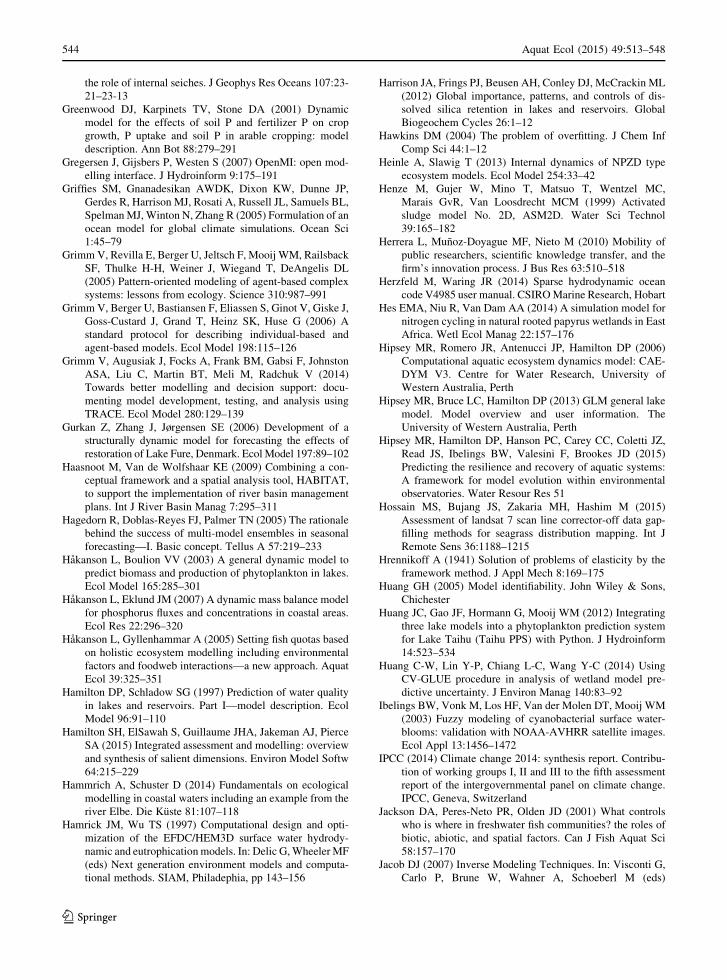
the role of internal seiches. J Geophys Res Oceans 107:23-
21–23-13
Greenwood DJ, Karpinets TV, Stone DA (2001) Dynamic
model for the effects of soil P and fertilizer P on crop
growth, P uptake and soil P in arable cropping: model
description. Ann Bot 88:279–291
Gregersen J, Gijsbers P, Westen S (2007) OpenMI: open mod-
elling interface. J Hydroinform 9:175–191
Griffies SM, Gnanadesikan AWDK, Dixon KW, Dunne JP,
Gerdes R, Harrison MJ, Rosati A, Russell JL, Samuels BL,
SpelmanMJ,Winton N, Zhang R (2005) Formulation of an
ocean model for global climate simulations. Ocean Sci
1:45–79
Grimm V, Revilla E, Berger U, Jeltsch F, Mooij WM, Railsback
SF, Thulke H-H, Weiner J, Wiegand T, DeAngelis DL
(2005) Pattern-oriented modeling of agent-based complex
systems: lessons from ecology. Science 310:987–991
Grimm V, Berger U, Bastiansen F, Eliassen S, Ginot V, Giske J,
Goss-Custard J, Grand T, Heinz SK, Huse G (2006) A
standard protocol for describing individual-based and
agent-based models. Ecol Model 198:115–126
Grimm V, Augusiak J, Focks A, Frank BM, Gabsi F, Johnston
ASA, Liu C, Martin BT, Meli M, Radchuk V (2014)
Towards better modelling and decision support: docu-
menting model development, testing, and analysis using
TRACE. Ecol Model 280:129–139
Gurkan Z, Zhang J, Jørgensen SE (2006) Development of a
structurally dynamic model for forecasting the effects of
restoration of Lake Fure, Denmark. EcolModel 197:89–102
Haasnoot M, Van de Wolfshaar KE (2009) Combining a con-
ceptual framework and a spatial analysis tool, HABITAT,
to support the implementation of river basin management
plans. Int J River Basin Manag 7:295–311
Hagedorn R, Doblas-Reyes FJ, Palmer TN (2005) The rationale
behind the success of multi-model ensembles in seasonal
forecasting—I. Basic concept. Tellus A 57:219–233
Hakanson L, Boulion VV (2003) A general dynamic model to
predict biomass and production of phytoplankton in lakes.
Ecol Model 165:285–301
Hakanson L, Eklund JM (2007) A dynamic mass balance model
for phosphorus fluxes and concentrations in coastal areas.
Ecol Res 22:296–320
Hakanson L, Gyllenhammar A (2005) Setting fish quotas based
on holistic ecosystem modelling including environmental
factors and foodweb interactions—a new approach. Aquat
Ecol 39:325–351
Hamilton DP, Schladow SG (1997) Prediction of water quality
in lakes and reservoirs. Part I—model description. Ecol
Model 96:91–110
Hamilton SH, ElSawah S, Guillaume JHA, Jakeman AJ, Pierce
SA (2015) Integrated assessment and modelling: overview
and synthesis of salient dimensions. Environ Model Softw
64:215–229
Hammrich A, Schuster D (2014) Fundamentals on ecological
modelling in coastal waters including an example from the
river Elbe. Die Kuste 81:107–118
Hamrick JM, Wu TS (1997) Computational design and opti-
mization of the EFDC/HEM3D surface water hydrody-
namic and eutrophicationmodels. In: Delic G,WheelerMF
(eds) Next generation environment models and computa-
tional methods. SIAM, Philadephia, pp 143–156
Harrison JA, Frings PJ, Beusen AH, Conley DJ, McCrackin ML
(2012) Global importance, patterns, and controls of dis-
solved silica retention in lakes and reservoirs. Global
Biogeochem Cycles 26:1–12
Hawkins DM (2004) The problem of overfitting. J Chem Inf
Comp Sci 44:1–12
Heinle A, Slawig T (2013) Internal dynamics of NPZD type
ecosystem models. Ecol Model 254:33–42
Henze M, Gujer W, Mino T, Matsuo T, Wentzel MC,
Marais GvR, Van Loosdrecht MCM (1999) Activated
sludge model No. 2D, ASM2D. Water Sci Technol
39:165–182
Herrera L, Munoz-Doyague MF, Nieto M (2010) Mobility of
public researchers, scientific knowledge transfer, and the
firm’s innovation process. J Bus Res 63:510–518
Herzfeld M, Waring JR (2014) Sparse hydrodynamic ocean
code V4985 user manual. CSIROMarine Research, Hobart
Hes EMA, Niu R, Van Dam AA (2014) A simulation model for
nitrogen cycling in natural rooted papyrus wetlands in East
Africa. Wetl Ecol Manag 22:157–176
Hipsey MR, Romero JR, Antenucci JP, Hamilton DP (2006)
Computational aquatic ecosystem dynamics model: CAE-
DYM V3. Centre for Water Research, University of
Western Australia, Perth
Hipsey MR, Bruce LC, Hamilton DP (2013) GLM general lake
model. Model overview and user information. The
University of Western Australia, Perth
Hipsey MR, Hamilton DP, Hanson PC, Carey CC, Coletti JZ,
Read JS, Ibelings BW, Valesini F, Brookes JD (2015)
Predicting the resilience and recovery of aquatic systems:
A framework for model evolution within environmental
observatories. Water Resour Res 51
Hossain MS, Bujang JS, Zakaria MH, Hashim M (2015)
Assessment of landsat 7 scan line corrector-off data gap-
filling methods for seagrass distribution mapping. Int J
Remote Sens 36:1188–1215
Hrennikoff A (1941) Solution of problems of elasticity by the
framework method. J Appl Mech 8:169–175
Huang GH (2005) Model identifiability. John Wiley & Sons,
Chichester
Huang JC, Gao JF, Hormann G, Mooij WM (2012) Integrating
three lake models into a phytoplankton prediction system
for Lake Taihu (Taihu PPS) with Python. J Hydroinform
14:523–534
Huang C-W, Lin Y-P, Chiang L-C, Wang Y-C (2014) Using
CV-GLUE procedure in analysis of wetland model pre-
dictive uncertainty. J Environ Manag 140:83–92
Ibelings BW, Vonk M, Los HF, Van der Molen DT, Mooij WM
(2003) Fuzzy modeling of cyanobacterial surface water-
blooms: validation with NOAA-AVHRR satellite images.
Ecol Appl 13:1456–1472
IPCC (2014) Climate change 2014: synthesis report. Contribu-
tion of working groups I, II and III to the fifth assessment
report of the intergovernmental panel on climate change.
IPCC, Geneva, Switzerland
Jackson DA, Peres-Neto PR, Olden JD (2001) What controls
who is where in freshwater fish communities? the roles of
biotic, abiotic, and spatial factors. Can J Fish Aquat Sci
58:157–170
Jacob DJ (2007) Inverse Modeling Techniques. In: Visconti G,
Carlo P, Brune W, Wahner A, Schoeberl M (eds)
544 Aquat Ecol (2015) 49:513–548
123
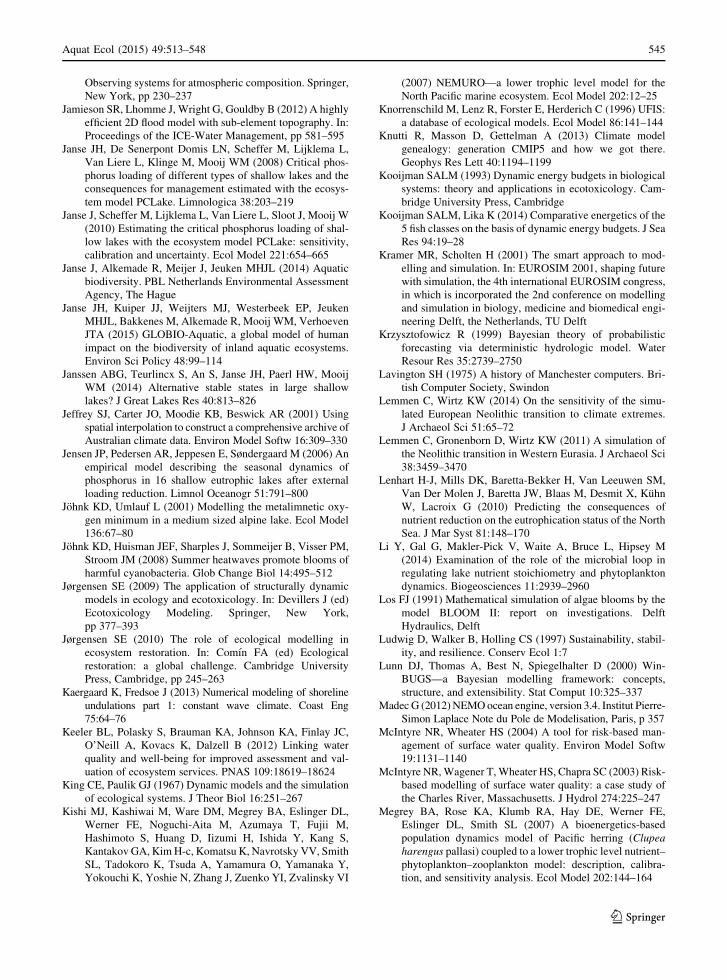
Observing systems for atmospheric composition. Springer,
New York, pp 230–237
Jamieson SR, Lhomme J, Wright G, Gouldby B (2012) A highly
efficient 2D flood model with sub-element topography. In:
Proceedings of the ICE-Water Management, pp 581–595
Janse JH, De Senerpont Domis LN, Scheffer M, Lijklema L,
Van Liere L, Klinge M, Mooij WM (2008) Critical phos-
phorus loading of different types of shallow lakes and the
consequences for management estimated with the ecosys-
tem model PCLake. Limnologica 38:203–219
Janse J, Scheffer M, Lijklema L, Van Liere L, Sloot J, Mooij W
(2010) Estimating the critical phosphorus loading of shal-
low lakes with the ecosystem model PCLake: sensitivity,
calibration and uncertainty. Ecol Model 221:654–665
Janse J, Alkemade R, Meijer J, Jeuken MHJL (2014) Aquatic
biodiversity. PBL Netherlands Environmental Assessment
Agency, The Hague
Janse JH, Kuiper JJ, Weijters MJ, Westerbeek EP, Jeuken
MHJL, Bakkenes M, Alkemade R, Mooij WM, Verhoeven
JTA (2015) GLOBIO-Aquatic, a global model of human
impact on the biodiversity of inland aquatic ecosystems.
Environ Sci Policy 48:99–114
Janssen ABG, Teurlincx S, An S, Janse JH, Paerl HW, Mooij
WM (2014) Alternative stable states in large shallow
lakes? J Great Lakes Res 40:813–826
Jeffrey SJ, Carter JO, Moodie KB, Beswick AR (2001) Using
spatial interpolation to construct a comprehensive archive of
Australian climate data. Environ Model Softw 16:309–330
Jensen JP, Pedersen AR, Jeppesen E, Søndergaard M (2006) An
empirical model describing the seasonal dynamics of
phosphorus in 16 shallow eutrophic lakes after external
loading reduction. Limnol Oceanogr 51:791–800
Johnk KD, Umlauf L (2001) Modelling the metalimnetic oxy-
gen minimum in a medium sized alpine lake. Ecol Model
136:67–80
Johnk KD, Huisman JEF, Sharples J, Sommeijer B, Visser PM,
Stroom JM (2008) Summer heatwaves promote blooms of
harmful cyanobacteria. Glob Change Biol 14:495–512
Jørgensen SE (2009) The application of structurally dynamic
models in ecology and ecotoxicology. In: Devillers J (ed)
Ecotoxicology Modeling. Springer, New York,
pp 377–393
Jørgensen SE (2010) The role of ecological modelling in
ecosystem restoration. In: Comın FA (ed) Ecological
restoration: a global challenge. Cambridge University
Press, Cambridge, pp 245–263
Kaergaard K, Fredsoe J (2013) Numerical modeling of shoreline
undulations part 1: constant wave climate. Coast Eng
75:64–76
Keeler BL, Polasky S, Brauman KA, Johnson KA, Finlay JC,
O’Neill A, Kovacs K, Dalzell B (2012) Linking water
quality and well-being for improved assessment and val-
uation of ecosystem services. PNAS 109:18619–18624
King CE, Paulik GJ (1967) Dynamic models and the simulation
of ecological systems. J Theor Biol 16:251–267
Kishi MJ, Kashiwai M, Ware DM, Megrey BA, Eslinger DL,
Werner FE, Noguchi-Aita M, Azumaya T, Fujii M,
Hashimoto S, Huang D, Iizumi H, Ishida Y, Kang S,
Kantakov GA, KimH-c, Komatsu K, Navrotsky VV, Smith
SL, Tadokoro K, Tsuda A, Yamamura O, Yamanaka Y,
Yokouchi K, Yoshie N, Zhang J, Zuenko YI, Zvalinsky VI
(2007) NEMURO—a lower trophic level model for the
North Pacific marine ecosystem. Ecol Model 202:12–25
Knorrenschild M, Lenz R, Forster E, Herderich C (1996) UFIS:
a database of ecological models. Ecol Model 86:141–144
Knutti R, Masson D, Gettelman A (2013) Climate model
genealogy: generation CMIP5 and how we got there.
Geophys Res Lett 40:1194–1199
Kooijman SALM (1993) Dynamic energy budgets in biological
systems: theory and applications in ecotoxicology. Cam-
bridge University Press, Cambridge
Kooijman SALM, Lika K (2014) Comparative energetics of the
5 fish classes on the basis of dynamic energy budgets. J Sea
Res 94:19–28
Kramer MR, Scholten H (2001) The smart approach to mod-
elling and simulation. In: EUROSIM 2001, shaping future
with simulation, the 4th international EUROSIM congress,
in which is incorporated the 2nd conference on modelling
and simulation in biology, medicine and biomedical engi-
neering Delft, the Netherlands, TU Delft
Krzysztofowicz R (1999) Bayesian theory of probabilistic
forecasting via deterministic hydrologic model. Water
Resour Res 35:2739–2750
Lavington SH (1975) A history of Manchester computers. Bri-
tish Computer Society, Swindon
Lemmen C, Wirtz KW (2014) On the sensitivity of the simu-
lated European Neolithic transition to climate extremes.
J Archaeol Sci 51:65–72
Lemmen C, Gronenborn D, Wirtz KW (2011) A simulation of
the Neolithic transition in Western Eurasia. J Archaeol Sci
38:3459–3470
Lenhart H-J, Mills DK, Baretta-Bekker H, Van Leeuwen SM,
Van Der Molen J, Baretta JW, Blaas M, Desmit X, Kuhn
W, Lacroix G (2010) Predicting the consequences of
nutrient reduction on the eutrophication status of the North
Sea. J Mar Syst 81:148–170
Li Y, Gal G, Makler-Pick V, Waite A, Bruce L, Hipsey M
(2014) Examination of the role of the microbial loop in
regulating lake nutrient stoichiometry and phytoplankton
dynamics. Biogeosciences 11:2939–2960
Los FJ (1991) Mathematical simulation of algae blooms by the
model BLOOM II: report on investigations. Delft
Hydraulics, Delft
Ludwig D, Walker B, Holling CS (1997) Sustainability, stabil-
ity, and resilience. Conserv Ecol 1:7
Lunn DJ, Thomas A, Best N, Spiegelhalter D (2000) Win-
BUGS—a Bayesian modelling framework: concepts,
structure, and extensibility. Stat Comput 10:325–337
MadecG (2012)NEMOocean engine, version 3.4. Institut Pierre-
Simon Laplace Note du Pole de Modelisation, Paris, p 357
McIntyre NR, Wheater HS (2004) A tool for risk-based man-
agement of surface water quality. Environ Model Softw
19:1131–1140
McIntyre NR,Wagener T,Wheater HS, Chapra SC (2003) Risk-
based modelling of surface water quality: a case study of
the Charles River, Massachusetts. J Hydrol 274:225–247
Megrey BA, Rose KA, Klumb RA, Hay DE, Werner FE,
Eslinger DL, Smith SL (2007) A bioenergetics-based
population dynamics model of Pacific herring (Clupea
harengus pallasi) coupled to a lower trophic level nutrient–
phytoplankton–zooplankton model: description, calibra-
tion, and sensitivity analysis. Ecol Model 202:144–164
Aquat Ecol (2015) 49:513–548 545
123
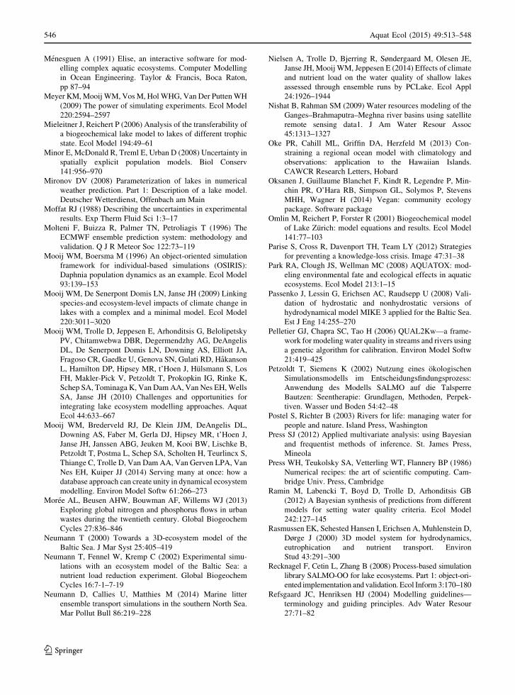
Menesguen A (1991) Elise, an interactive software for mod-
elling complex aquatic ecosystems. Computer Modelling
in Ocean Engineering. Taylor & Francis, Boca Raton,
pp 87–94
Meyer KM,Mooij WM, VosM, HolWHG, Van Der PuttenWH
(2009) The power of simulating experiments. Ecol Model
220:2594–2597
Mieleitner J, Reichert P (2006) Analysis of the transferability of
a biogeochemical lake model to lakes of different trophic
state. Ecol Model 194:49–61
Minor E, McDonald R, Treml E, Urban D (2008) Uncertainty in
spatially explicit population models. Biol Conserv
141:956–970
Mironov DV (2008) Parameterization of lakes in numerical
weather prediction. Part 1: Description of a lake model.
Deutscher Wetterdienst, Offenbach am Main
Moffat RJ (1988) Describing the uncertainties in experimental
results. Exp Therm Fluid Sci 1:3–17
Molteni F, Buizza R, Palmer TN, Petroliagis T (1996) The
ECMWF ensemble prediction system: methodology and
validation. Q J R Meteor Soc 122:73–119
Mooij WM, Boersma M (1996) An object-oriented simulation
framework for individual-based simulations (OSIRIS):
Daphnia population dynamics as an example. Ecol Model
93:139–153
Mooij WM, De Senerpont Domis LN, Janse JH (2009) Linking
species-and ecosystem-level impacts of climate change in
lakes with a complex and a minimal model. Ecol Model
220:3011–3020
Mooij WM, Trolle D, Jeppesen E, Arhonditsis G, Belolipetsky
PV, Chitamwebwa DBR, Degermendzhy AG, DeAngelis
DL, De Senerpont Domis LN, Downing AS, Elliott JA,
Fragoso CR, Gaedke U, Genova SN, Gulati RD, Hakanson
L, Hamilton DP, Hipsey MR, t’Hoen J, Hulsmann S, Los
FH, Makler-Pick V, Petzoldt T, Prokopkin IG, Rinke K,
Schep SA, Tominaga K, Van DamAA, Van Nes EH,Wells
SA, Janse JH (2010) Challenges and opportunities for
integrating lake ecosystem modelling approaches. Aquat
Ecol 44:633–667
Mooij WM, Brederveld RJ, De Klein JJM, DeAngelis DL,
Downing AS, Faber M, Gerla DJ, Hipsey MR, t’Hoen J,
Janse JH, Janssen ABG, Jeuken M, Kooi BW, Lischke B,
Petzoldt T, Postma L, Schep SA, Scholten H, Teurlincx S,
Thiange C, Trolle D, Van Dam AA, Van Gerven LPA, Van
Nes EH, Kuiper JJ (2014) Serving many at once: how a
database approach can create unity in dynamical ecosystem
modelling. Environ Model Softw 61:266–273
Moree AL, Beusen AHW, Bouwman AF, Willems WJ (2013)
Exploring global nitrogen and phosphorus flows in urban
wastes during the twentieth century. Global Biogeochem
Cycles 27:836–846
Neumann T (2000) Towards a 3D-ecosystem model of the
Baltic Sea. J Mar Syst 25:405–419
Neumann T, Fennel W, Kremp C (2002) Experimental simu-
lations with an ecosystem model of the Baltic Sea: a
nutrient load reduction experiment. Global Biogeochem
Cycles 16:7-1–7-19
Neumann D, Callies U, Matthies M (2014) Marine litter
ensemble transport simulations in the southern North Sea.
Mar Pollut Bull 86:219–228
Nielsen A, Trolle D, Bjerring R, Søndergaard M, Olesen JE,
Janse JH, Mooij WM, Jeppesen E (2014) Effects of climate
and nutrient load on the water quality of shallow lakes
assessed through ensemble runs by PCLake. Ecol Appl
24:1926–1944
Nishat B, Rahman SM (2009) Water resources modeling of the
Ganges–Brahmaputra–Meghna river basins using satellite
remote sensing data1. J Am Water Resour Assoc
45:1313–1327
Oke PR, Cahill ML, Griffin DA, Herzfeld M (2013) Con-
straining a regional ocean model with climatology and
observations: application to the Hawaiian Islands.
CAWCR Research Letters, Hobard
Oksanen J, Guillaume Blanchet F, Kindt R, Legendre P, Min-
chin PR, O’Hara RB, Simpson GL, Solymos P, Stevens
MHH, Wagner H (2014) Vegan: community ecology
package. Software package
Omlin M, Reichert P, Forster R (2001) Biogeochemical model
of Lake Zurich: model equations and results. Ecol Model
141:77–103
Parise S, Cross R, Davenport TH, Team LY (2012) Strategies
for preventing a knowledge-loss crisis. Image 47:31–38
Park RA, Clough JS, Wellman MC (2008) AQUATOX: mod-
eling environmental fate and ecological effects in aquatic
ecosystems. Ecol Model 213:1–15
Passenko J, Lessin G, Erichsen AC, Raudsepp U (2008) Vali-
dation of hydrostatic and nonhydrostatic versions of
hydrodynamical model MIKE 3 applied for the Baltic Sea.
Est J Eng 14:255–270
Pelletier GJ, Chapra SC, Tao H (2006) QUAL2Kw—a frame-
work for modeling water quality in streams and rivers using
a genetic algorithm for calibration. Environ Model Softw
21:419–425
Petzoldt T, Siemens K (2002) Nutzung eines okologischen
Simulationsmodells im Entscheidungsfindungsprozess:
Anwendung des Modells SALMO auf die Talsperre
Bautzen: Seentherapie: Grundlagen, Methoden, Perpek-
tiven. Wasser und Boden 54:42–48
Postel S, Richter B (2003) Rivers for life: managing water for
people and nature. Island Press, Washington
Press SJ (2012) Applied multivariate analysis: using Bayesian
and frequentist methods of inference. St. James Press,
Mineola
Press WH, Teukolsky SA, Vetterling WT, Flannery BP (1986)
Numerical recipes: the art of scientific computing. Cam-
bridge Univ. Press, Cambridge
Ramin M, Labencki T, Boyd D, Trolle D, Arhonditsis GB
(2012) A Bayesian synthesis of predictions from different
models for setting water quality criteria. Ecol Model
242:127–145
Rasmussen EK, Sehested Hansen I, Erichsen A, Muhlenstein D,
Dørge J (2000) 3D model system for hydrodynamics,
eutrophication and nutrient transport. Environ
Stud 43:291–300
Recknagel F, Cetin L, Zhang B (2008) Process-based simulation
library SALMO-OO for lake ecosystems. Part 1: object-ori-
ented implementation and validation. Ecol Inform3:170–180
Refsgaard JC, Henriksen HJ (2004) Modelling guidelines—
terminology and guiding principles. Adv Water Resour
27:71–82
546 Aquat Ecol (2015) 49:513–548
123
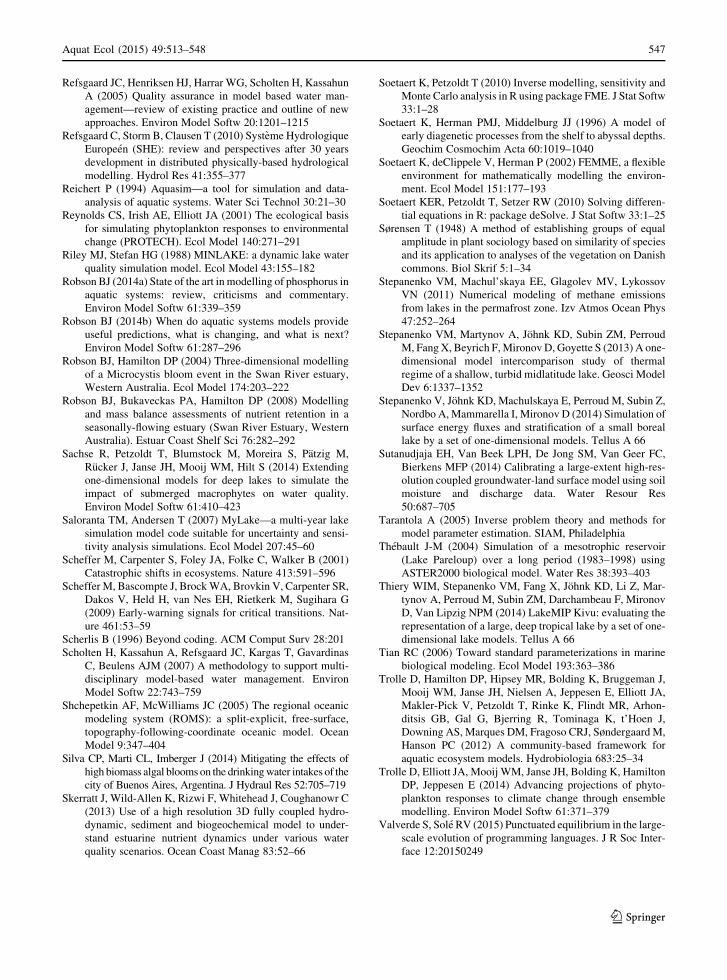
Refsgaard JC, Henriksen HJ, Harrar WG, Scholten H, Kassahun
A (2005) Quality assurance in model based water man-
agement—review of existing practice and outline of new
approaches. Environ Model Softw 20:1201–1215
Refsgaard C, Storm B, Clausen T (2010) Systeme Hydrologique
Europeen (SHE): review and perspectives after 30 years
development in distributed physically-based hydrological
modelling. Hydrol Res 41:355–377
Reichert P (1994) Aquasim—a tool for simulation and data-
analysis of aquatic systems. Water Sci Technol 30:21–30
Reynolds CS, Irish AE, Elliott JA (2001) The ecological basis
for simulating phytoplankton responses to environmental
change (PROTECH). Ecol Model 140:271–291
Riley MJ, Stefan HG (1988) MINLAKE: a dynamic lake water
quality simulation model. Ecol Model 43:155–182
Robson BJ (2014a) State of the art in modelling of phosphorus in
aquatic systems: review, criticisms and commentary.
Environ Model Softw 61:339–359
Robson BJ (2014b) When do aquatic systems models provide
useful predictions, what is changing, and what is next?
Environ Model Softw 61:287–296
Robson BJ, Hamilton DP (2004) Three-dimensional modelling
of a Microcystis bloom event in the Swan River estuary,
Western Australia. Ecol Model 174:203–222
Robson BJ, Bukaveckas PA, Hamilton DP (2008) Modelling
and mass balance assessments of nutrient retention in a
seasonally-flowing estuary (Swan River Estuary, Western
Australia). Estuar Coast Shelf Sci 76:282–292
Sachse R, Petzoldt T, Blumstock M, Moreira S, Patzig M,
Rucker J, Janse JH, Mooij WM, Hilt S (2014) Extending
one-dimensional models for deep lakes to simulate the
impact of submerged macrophytes on water quality.
Environ Model Softw 61:410–423
Saloranta TM, Andersen T (2007) MyLake—a multi-year lake
simulation model code suitable for uncertainty and sensi-
tivity analysis simulations. Ecol Model 207:45–60
Scheffer M, Carpenter S, Foley JA, Folke C, Walker B (2001)
Catastrophic shifts in ecosystems. Nature 413:591–596
Scheffer M, Bascompte J, BrockWA, Brovkin V, Carpenter SR,
Dakos V, Held H, van Nes EH, Rietkerk M, Sugihara G
(2009) Early-warning signals for critical transitions. Nat-
ure 461:53–59
Scherlis B (1996) Beyond coding. ACM Comput Surv 28:201
Scholten H, Kassahun A, Refsgaard JC, Kargas T, Gavardinas
C, Beulens AJM (2007) A methodology to support multi-
disciplinary model-based water management. Environ
Model Softw 22:743–759
Shchepetkin AF, McWilliams JC (2005) The regional oceanic
modeling system (ROMS): a split-explicit, free-surface,
topography-following-coordinate oceanic model. Ocean
Model 9:347–404
Silva CP, Marti CL, Imberger J (2014) Mitigating the effects of
high biomass algal blooms on the drinkingwater intakes of the
city of Buenos Aires, Argentina. J Hydraul Res 52:705–719
Skerratt J, Wild-Allen K, Rizwi F, Whitehead J, Coughanowr C
(2013) Use of a high resolution 3D fully coupled hydro-
dynamic, sediment and biogeochemical model to under-
stand estuarine nutrient dynamics under various water
quality scenarios. Ocean Coast Manag 83:52–66
Soetaert K, Petzoldt T (2010) Inverse modelling, sensitivity and
Monte Carlo analysis in R using package FME. J Stat Softw
33:1–28
Soetaert K, Herman PMJ, Middelburg JJ (1996) A model of
early diagenetic processes from the shelf to abyssal depths.
Geochim Cosmochim Acta 60:1019–1040
Soetaert K, deClippele V, Herman P (2002) FEMME, a flexible
environment for mathematically modelling the environ-
ment. Ecol Model 151:177–193
Soetaert KER, Petzoldt T, Setzer RW (2010) Solving differen-
tial equations in R: package deSolve. J Stat Softw 33:1–25
Sørensen T (1948) A method of establishing groups of equal
amplitude in plant sociology based on similarity of species
and its application to analyses of the vegetation on Danish
commons. Biol Skrif 5:1–34
Stepanenko VM, Machul’skaya EE, Glagolev MV, Lykossov
VN (2011) Numerical modeling of methane emissions
from lakes in the permafrost zone. Izv Atmos Ocean Phys
47:252–264
Stepanenko VM, Martynov A, Johnk KD, Subin ZM, Perroud
M, FangX, Beyrich F,Mironov D, Goyette S (2013) A one-
dimensional model intercomparison study of thermal
regime of a shallow, turbid midlatitude lake. Geosci Model
Dev 6:1337–1352
Stepanenko V, Johnk KD, Machulskaya E, Perroud M, Subin Z,
Nordbo A, Mammarella I, Mironov D (2014) Simulation of
surface energy fluxes and stratification of a small boreal
lake by a set of one-dimensional models. Tellus A 66
Sutanudjaja EH, Van Beek LPH, De Jong SM, Van Geer FC,
Bierkens MFP (2014) Calibrating a large-extent high-res-
olution coupled groundwater-land surface model using soil
moisture and discharge data. Water Resour Res
50:687–705
Tarantola A (2005) Inverse problem theory and methods for
model parameter estimation. SIAM, Philadelphia
Thebault J-M (2004) Simulation of a mesotrophic reservoir
(Lake Pareloup) over a long period (1983–1998) using
ASTER2000 biological model. Water Res 38:393–403
Thiery WIM, Stepanenko VM, Fang X, Johnk KD, Li Z, Mar-
tynov A, Perroud M, Subin ZM, Darchambeau F, Mironov
D, Van Lipzig NPM (2014) LakeMIP Kivu: evaluating the
representation of a large, deep tropical lake by a set of one-
dimensional lake models. Tellus A 66
Tian RC (2006) Toward standard parameterizations in marine
biological modeling. Ecol Model 193:363–386
Trolle D, Hamilton DP, Hipsey MR, Bolding K, Bruggeman J,
Mooij WM, Janse JH, Nielsen A, Jeppesen E, Elliott JA,
Makler-Pick V, Petzoldt T, Rinke K, Flindt MR, Arhon-
ditsis GB, Gal G, Bjerring R, Tominaga K, t’Hoen J,
Downing AS, Marques DM, Fragoso CRJ, Søndergaard M,
Hanson PC (2012) A community-based framework for
aquatic ecosystem models. Hydrobiologia 683:25–34
Trolle D, Elliott JA, Mooij WM, Janse JH, Bolding K, Hamilton
DP, Jeppesen E (2014) Advancing projections of phyto-
plankton responses to climate change through ensemble
modelling. Environ Model Softw 61:371–379
Valverde S, Sole RV (2015) Punctuated equilibrium in the large-
scale evolution of programming languages. J R Soc Inter-
face 12:20150249
Aquat Ecol (2015) 49:513–548 547
123
Van Beek LPH, Wada Y, Bierkens MFP (2011) Global monthly
water stress: 1.Water balance and water availability. Water
Resour Res 47
Van Dam AA, Dardona A, Kelderman P, Kansiime F (2007) A
simulation model for nitrogen retention in a papyrus wet-
land near Lake Victoria, Uganda (East Africa). Wetl Ecol
Manag 15:469–480
Van Der Heide T, Van Nes EH, Geerling GW, Smolders AJP,
Bouma TJ, Van Katwijk MM (2007) Positive feedbacks in
seagrass ecosystems: implications for success in conser-
vation and restoration. Ecosystems 10:1311–1322
Van Gerven LPA, Brederveld RJ, De Klein JJM, DeAngelis DL,
Downing AS, Faber M, Gerla DJ, ’t Hoen J, Janse JH,
Janssen ABG, Jeuken M, Kooi BW, Kuiper JJ, Lischke B,
Liu S, Petzoldt T, Schep SA, Teurlincx S, Thiange C,
Trolle D, Van Nes EH, Mooij WM (2015) Advantages of
concurrent use of multiple software frameworks in water
quality modelling using a database approach. Fund Appl
Limnol 186:5–20
Van Liere L, Janse JH, Arts GHP (2007) Setting critical nutrient
values for ditches using the eutrophication model PCDitch.
Aquat Ecol 41:443–449
Van Nes EH, Lammens EHRR, Scheffer M (2002a) PISCA-
TOR, an individual-based model to analyze the dynamics
of lake fish communities. Ecol Model 152:261–278
Van Nes EH, Scheffer M, Van den Berg MS, Coops H (2002b)
Dominance of charophytes in eutrophic shallow lakes—
when should we expect it to be an alternative stable state?
Aquat Bot 72:275–296
Van Oevelen D, Van Den Meersche K, Meysman FJR, Soetaert
K, Middelburg JJ, Vezina AF (2010) Quantifying food web
flows using linear inverse models. Ecosystems 13:32–45
Vezina AF, Platt T (1988) Food web dynamics in the ocean. 1.
Best-estimates of flow networks using inverse methods.
Mar Ecol Prog Ser 42:269–287
Vollenweider RA (1975) Input–output models. Schweiz Z
Hydrol 37:53–84
Wade AJ, Durand P, Beaujouan V, Wessel WW, Raat KJ,
Whitehead PG, Butterfield D, Rankinen K, Lepisto A
(2002) A nitrogen model for European catchments: INCA,
new model structure and equations. Hydrol Earth Syst Sci
6:559–582
Weijerman M, Fulton EA, Janssen ABG, Kuiper JJ, Leemans R,
Robson BJ (2015) How models can support ecosystem-
based management of coral reefs. Prog Oceanogr. doi:10.
1016/j.pocean.2014.12.017
Wijesekara GN, Farjad B, Gupta A, Qiao Y, Delaney P, Mar-
ceau DJ (2014) A comprehensive land-use/hydrological
modeling system for scenario simulations in the Elbow
River watershed, Alberta, Canada. Environ Manag
53:357–381
Wild-Allen K,HerzfeldM, Thompson PA, RosebrockU, Parslow
J, Volkman JK (2010) Applied coastal biogeochemical
modelling to quantify the environmental impact of fish farm
nutrients and inform managers. J Mar Syst 81:134–147
Wilks DS (2002) Smoothing forecast ensembles with fitted
probability distributions. Q J RMeteor Soc 128:2821–2836
Wu TS, Hamrick JM, McCutcheon SC, Ambrose RB (1997)
Benchmarking the EFDC/HEM3D surface water hydro-
dynamic and eutrophication models. In: Delic G, Wheeler
MF (eds) Next generation environment models and com-
putational methods. SIAM, Philadelphia, pp 157–161
Xiao Y, Friedrichs MAM (2014) Using biogeochemical data
assimilation to assess the relative skill of multiple
ecosystem models: effects of increasing the complexity of
the planktonic food web. Biogeosciences 11:481–520
Xu F-L, Tao S, Dawson R, Li P-g, Cao J (2001) Lake ecosystem
health assessment: indicators and methods. Water Res
35:3157–3167
Xu F, Yang ZF, Chen B, Zhao YW (2013) Impact of submerged
plants on ecosystem health of the plant-dominated
Baiyangdian Lake, China. Ecol Model 252:167–175
Yakushev E, Protsenko EA, Bruggeman J (2014) Bottom
RedOx Model (BROM) general description and applica-
tion for seasonal anoxia simulations. Norwegian Institute
for water Research (NIVA), Oslo
548 Aquat Ecol (2015) 49:513–548
123
Recommended