Experiments on Decisions Under Uncertainty: A Theoretical Framework
Eran Shmaya ∗ Leeat Yariv†‡
Current Version: November 11, 2015
Abstract. The analysis of lab data entails a joint test of the underlying theory
and of subjects’conjectures regarding the experimental design itself, how subjects frame
the experiment. We provide a theoretical framework for analyzing such conjectures. We
use experiments of decision making under uncertainty as a case study. Absent restric-
tions on subjects’framing of the experiment, we show that any behavior is consistent
with standard updating ("anything goes"), including that suggestive of anomalies such
as over-confidence, excess belief stickiness, etc. When the experimental protocol restricts
subjects’conjectures (plausibly, by generating information during the experiment), stan-
dard updating has non-trivial testable implications.
JEL classification: D01, D80, D83.
Keywords: Bayesian Updating, Experimental Design, Conjectured Experiments.
∗Managerial Economics and Decision Sciences (MEDS), Kellogg School of Management, NorthwesternUniversity, Evanston, IL 60208, USA. e-mail: [email protected]†Division of the Humanities and Social Sciences, Caltech, Pasadena, CA 91125, USA. e-mail:
[email protected]‡We thank Alessandro Lizzeri for numerous comments on an earlier version of the paper. Christopher
Chambers, Federico Echenique, Matthew Jackson, the coeditor, and three anonymous referees provided veryhelpful suggestions. Financial support from the National Science Foundation (SES 0963583) and the Gordonand Betty Moore Foundation is gratefully acknowledged.

Experiments on Decisions Under Uncertainty: A Theoretical Framework 1
1. Overview
1.1 Introduction
Experiments studying behavior under uncertainty (be it regarding some underlying state,
such as income in consumption-saving problems, or regarding others’behavior, as is the case
in practically all strategic interactions) usually consist of three stages. First, the uncertainty is
realized; Second, subjects are provided with partial information about that realization; Third,
subjects choose an action. When analyzing data of such experiments, one essentially tests
joint hypotheses regarding responses to the experimental design (namely, the realization of
uncertainty and the information generation procedure) and subjects’beliefs about the design
itself. The focus of this paper is the analysis of the potential consequences of such joint tests.
We allow subjects to hold arbitrary conjectures about the experimental design and identify
links between classes of conjectures subjects hold and the testable implications of theoretical
predictions in the lab.
The idea that subjects may form (potentially inaccurate) beliefs about an experiment’s
design to which they respond is long standing in the social sciences. It falls under the general
umbrella of experimenter demand, suggesting that the design itself makes subjects (consciously
or subconsciously) frame the problem at hand in a particular way that makes them believe cer-
tain responses are more appropriate than others. It has not only been a concern for economists
(Zizzo, 2010, and references therein). It is also considered a potential source of distortion in
responses to psychological surveys (see Paulhus, 1991) and a channel through which subjects
in sociological experiments choose their actions (see Gillespie, 1991). Experimenter demand
may even play a role in the generation of placebo effects in medicine (see Beecher, 1955 and
work that followed). Despite its importance for experimental deductions, the literature has
offered little in the form of a theoretical framework for inspecting the testable implications of
experiments accounting for experimenter demand effects. Our goal is to take a step in that
direction.
We concentrate on a general case study of laboratory decision making under uncertainty.
Most experiments in this class involve some form of updating. Consequently, a natural first
step in the theoretical analysis of such experiments pertains to experiments having to do with

Experiments on Decisions Under Uncertainty: A Theoretical Framework 2
elicitation of beliefs, which are the experiments we study in this paper.
We consider experiments in which payoffs depend on some unknown state. After the state
is realized, a subject is provided with some information regarding the state in the form of
a sequence of potentially informative signals. Ultimately, the subject chooses one of several
alternatives. Many extant experiments fall under this category (particularly when thinking of
other subjects’actions as part of the state). For instance, consumption-saving experiments,
individual experimentation and learning experiments, herding, and sequential voting exper-
iments all naturally fall under this rubric (see, for example, Kagel and Roth, 1997 for an
overview of experiments in different fields of economics).
1.2 A Motivating Example
Before describing our formal results, consider the following example, providing a simple
caricature of the structure of experiments of decision making under uncertainty.
There are two states of nature, a and b, realized at the outset of the experiment. For
example, a and b can stand for whether or not going on vacation is a good idea, as in Tversky
and Shafir’s (1992) disjunction effect experiments. The subject’s goal is to report which
of the states is most likely given different amounts of information.1 For simplicity, assume
that initially, she is given no information. Then she receives some information, say in the
form of a signal taking the values u or d. For example, in Tversky and Shafir’s (1992)
experiments subjects were asked to contemplate either failing or passing an important exam.
Figure 1 captures, up to relabeling, the three types of responses one could observe in such
an experiment. The actions at the roots of each tree correspond to the reports absent any
signals, while actions at the other two nodes correspond to the subject’s responses following
the respective signals.
In panel (1), the subject does not change her mind regardless of which signal she observes.
This is consistent with Bayesian updating. For instance, the subject may have a strong prior
favoring the state a and view the signals as uninformative. In panel (2), the subject changes
her mind when the signal is d. This can also be explained with Bayesian updating by assuming,
1For instance, she may be paid a fixed amount only when her response matches the realized state.

Experiments on Decisions Under Uncertainty: A Theoretical Framework 3
us =1
ds =1
a
a
a
us =1
ds =1
a
a
us =1
ds =1
b
(1) (2)
(3)
b
a
a
Figure 1: Simple Reversal
e.g., that the prior for a is p > 1/2 while the signal s1 follows the following distribution:
P (s1 = u | a) = P (s1 = d | b) = q and P (s1 = d | a) = P (s1 = u | b) = 1− q,
where q > p. Thus, upon observing the signal u, the subject views a as more likely and upon
observing the signal d, the subject views the state b as more likely.2
Panel (3) describes a situation in which regardless of what the signal is, the subject changes
her view of what is the most likely state. These observations cannot be explained with
simple Bayesian updating. Indeed, if the subject updates in a standard manner, absent any
information, she must put some weight on the realization of s1 being u and complementary
weight on the realization of s1 being d. In particular, her belief that the state is a when she
does not observe a signal must be a convex combination of her beliefs following the realization
of the signal. Thus, unless the subject is indifferent, a belief that puts weight lower than 1/2
on the state a must be a convex combination of two beliefs that put weight greater than 1/2
on the state a, which is not possible.3
2In fact, one can come up with many belief structures for the subject that would be consistent with theobserved reports and Bayesian updating for either Panel (1) or Panel (2).
3This is reminiscent of a simple violation of Savage’s (1954) “Sure Thing Principle.”We elaborate on thecomparison below (see Section 3).

Experiments on Decisions Under Uncertainty: A Theoretical Framework 4
In fact, many experiments that are used to illustrate updating anomalies exhibit obser-
vations of the form of Panel (3) —Tversky and Shafir’s (1992) disjunction effect experiments
take this format4, as do an assortment of experiments on over-confidence, belief polarization,
etc. (for an overview, see, e.g., Camerer, Loewenstein, and Rabin, 2006 or Nisbett and Ross,
1980).
To summarize, even without placing any restrictions on the subject’s belief about the
initial distribution of states and the signal generation process, Bayesian updating has clear
testable implications. Panels (1) and (2) can be explained, while Panel (3) cannot.
In the current paper we also entertain the idea that the subject conjectures the amount
of information revealed to her by the experimenter is a function of the realized uncertainty:
the state and the signals. Then, Panel (3) can easily be explained with Bayesian updating
with such richer conjectures. For instance, the subject could conjecture that a-priori the
states are equally likely, but that when the state is b (or when the appropriate response is
b), the experimenter does not reveal any information to her, while when the state is a, the
experimenter reveals either signal with equal probability. In particular, behavior that seems
to suggest anomalous updating procedures may be attributed to the subject’s framing of the
experiment instead.
Nonetheless, note that in explaining Panel (3), we only need the subject to conjecture the
amount of information depends on the realized state (and not necessarily on the realized sig-
nals). Such restricted conjectures are relevant for experiments of decisions under uncertainty
in which there is transparency regarding how signals are generated (for example, signals may
be generated during the experiment, after their number had been determined, as is common
practice in, e.g., voting experiments). Interestingly, they do entail testable implications.
Consider Figure 2 that illustrates reports from an experiment as above in which there are
two signal realizations, each taking the value of u or d. Note that the sub-tree corresponding
to s1 = u is of the form appearing in Panel (3) of Figure 1. In particular, in order to explain
4Specifically, Tversky and Shafir (1992) asked students whether they would be interested in a vacationpackage that would take place after the results of an exam would be revealed. 32% of the subjects wereinterested, 7% of the subjects were not interested, and the remaining 61% were willing to pay $5 to havethe option to cancel the vacation after realizing whether they had passed or failed. Nonetheless, when askedwhether they would buy the same vacation package after discovering they had failed or passed the exam, 57%or 54%, resepectively, of the subjects reported affi rmatively.

Experiments on Decisions Under Uncertainty: A Theoretical Framework 5
Figure 2: Reversal Not Explained by a Partially Restricted Conjectured Experiment
the reversal following either signal s2, we need to assume the subject conjectures that the mere
observation of two signals is more likely when the state is b. However, switch to the other
sub-tree corresponding to s1 = d. Here, we see a similar reversal, but now the subject reports
the state a regardless of s2. The only way to explain this would be with a conjecture that
makes the observation of two signals more likely when the state is a. It is therefore impossible
to explain these observations with such restricted conjectures. Thus, transparency of the
signal generation procedure assures that Bayesian updating has clear testable implications,
even without restricting the subject’s conjecture on the distribution of the underlying state,
signal generation process, and the experimenter’s strategy of information revelation (that may
depend on the realized state).
This example highlights two important methodological messages of the paper. First, when
no restrictions are placed on subjects’framing of the experiment, any behavior is consistent
with standard updating (“anything goes”). Second, when the experimental protocol restricts
subjects’conjectures (say, by generating information during the experiment), standard up-
dating entails non-trivial testable implications. Namely, such protocols restrict the type of
action reversals that Bayesian subjects may exhibit when they are provided with additional
information.

Experiments on Decisions Under Uncertainty: A Theoretical Framework 6
1.3 Description of Results
In general, the design of an experiment dictates how much information, i.e., the number
of signals, subjects observe prior to making choices. Subjects may hold a wide range of
beliefs regarding the link between the amount of information they observe and the underlying
uncertainty. We use the term conjectured experiment to denote the subject’s beliefs about the
design of the experiment. We study the impacts of two types of conjectured experiments: one
in which the amount of information is perceived independent of any realized uncertainty and
another in which the amount of information can be correlated (in an arbitrary manner) with
the realized uncertainty.
We emphasize that in experiments of decision making under uncertainty, the amount of
information per-se is usually independent of the actual state and the signals’ realizations.
There are many reasons why a subject’s conjecture may not coincide with the actual experi-
mental design. For instance, subjects may arrive at the lab with real-world recipes of behavior
that affect their interpretation of experimental instructions, subjects may misunderstand the
notion of independence, or theorize about the experimenter’s goals and selective choice of in-
formation (see Friedman and Sunder, 1994, Kagel and Roth, 1997, and Zizzo, 2010). Subjects’
conjectures do not reflect suspicions regarding how the experiment is carried out.5
We assume subjects report to the experimenter the state they view as most likely. This
is a natural starting point for our analysis since looking at reports of the most likely state
requires the subject to go through very simple calculations that do not require expected utility
maximization. The entire analysis here is based on ordinal utilities (a monotonic transforma-
tion of the subject’s utility will not change her optimal response). In particular, the analysis
is not sensitive to subjects’risk preferences. In contrast, in order to elicit the full beliefs a
subject holds, choosing the proper utility would require certain behavioral assumptions, e.g.,
a quadratic scoring rule combined with maximization of expected utility.
Suppose first that subjects’conjectured experiments are restricted so that the amount of
information revealed to them is independent of both the realized state and the realized signals.
5Indeed, most economic experiments are preceded by a set of instructions, and the prevailing norm in theprofession banning deception would presumably trickle down to subjects.

Experiments on Decisions Under Uncertainty: A Theoretical Framework 7
In that case, there is a natural restriction on subjects’reports for them to be consistent with
Bayesian updating (generalizing our introductory example). Indeed, Theorem 1 shows that
the subject is Bayesian if and only if the following condition holds: The subject chooses the
action a for signal sequence s whenever all continuation signal sequences lead her to choose
a.6
The other polar case of subjects’ conjectures occurs when no restrictions are put and
subjects’conjectures are allowed to entail correlations between the realization of all uncertainty
(on the state and signals) and the number of signals observed; Subjects are free to frame the
experiment however way they like. In that case, in line with the example above, Theorem 2
illustrates an “anything goes”result —any responses of subjects can be explained as arising
from a particular conjectured experiment and Bayesian updating of the released information.
In other words, in that case the theoretical predictions have no bite once jointly tested with
the conjectured experiment.
From a positive and prescriptive point of view, certain experimental protocols are likely to
place restrictions on the conjectures subjects hold. For instance, in many voting experiments,
the number of signals is determined at the outset, but subjects produce their own signals, e.g.,
by drawing a ball from a physical urn (the composition of which represents the underlying
state), during the experiment.7 In terms of the subjects’conjectures, such designs are likely
to entail independence between the realized signals and the number of signals provided.
In Section 5 we study the intermediate case in which subjects’conjectures allow for cor-
relations between the amount of information revealed and realized state, but the amount of
information is independent of the signal realizations. Such partially restricted conjectures
allow for the volume of information to be associated with the state realization. Theorem
3 generalizes the example corresponding to Figure 2 and provides a characterization of the
class of reversals that violate Bayesian updating when subjects hold partially restricted con-
jectures. Much as in the example, the reversals that are consistent with Bayesian updating
6This is reminiscent of the “Sure Thing Principle”a-la Savage (1954) and dynamic consistency. However,the experimental observations are mappings from sequences of signals. Thus, they consist a subset of elementsconsidered by the Savage (1954) type of analysis. In particular, the suffi ciency of the condition cannot bededuced from the work on foundations of expected utility. We elaborate on this point in Section 3.
7See Palfrey (2006) for a description of various experiments on voting behavior.

Experiments on Decisions Under Uncertainty: A Theoretical Framework 8
are roughly described by going “in the same direction”(or tending to a specific report) for a
particular length of signal sequence. The theorem provides the tools for deducing departures
from Bayesian updating when the signal generation process is transparent in the lab.
The underlying assumption in our analysis is that there is a natural sequencing of signals.
This is why the experimental design is captured by the number of signals reported to the
subject. This assumption is applicable in many situations (indeed, any context in which
signals are tied with time), and eases the presentation. In the Online Appendix we provide
a similar analysis for environments in which there is no natural ordering of signals and a
general conjectured experiment pertains to the dimensions of information that are reported
(or which elements of the set of signals are reported) and their correlation with the underlying
uncertainty.8
As mentioned, our analysis is very closely related to the unformalized notion of experi-
menter demand, the idea that the design itself makes subjects (consciously or subconsciously)
frame the problem at hand in a particular way that makes them believe certain responses are
more appropriate than others (see, e.g., Friedman and Sunder, 1994, Kagel and Roth, 1997,
and Zizzo, 2010). Experimenter demand type of arguments broadly take one of two forms.
The first suggests that the way the experimenter phrases problems indicates something to
the subject about the realized uncertainty and the correct response. The second refers to the
subject trying to “help”or “satisfy”the experimenter by aiming at the answers the experi-
menter is seeking. Our approach provides a first step in formalizing the former manifestation
of experimenter demand, by contemplating a large class of conjectures, or ways to frame the
experimental design. It is a necessary step for future models of the second demand manifes-
tation as well, that potentially requires more behavioral and strategic assumptions on both
experimenter and subject.
The idea that individuals may exhibit a variety of non-standard behaviors in the presence
of uncertainty, such as excess stickiness of beliefs, over-confidence, etc., has received much
8Our “anything goes” result still holds when conjectured experiments are unrestricted. However, theimplications imposed by the natural analogue of restricted conjectured experiments do not carry through.In fact, we identify stronger observational restrictions that are in the spirit of “Dutch books.”Experimentalobservations can be explained if and only if, after observing the subjects’responses, the experimenter cannotdesign a sequence of bets that would lead the agent to lose money for sure.

Experiments on Decisions Under Uncertainty: A Theoretical Framework 9
attention in both psychology and economics (see, for example, Part 1 in Brocas and Carrillo,
2004, Kahneman, Slovic, and Tversky, 1982, and Nisbett and Ross, 1980).9 The economics
literature has taken two approaches for utilizing these observations:
1. Suggest alternative models of belief updating to that prescribed by Bayes’ rule (e.g.,
Rabin and Schrag, 1999 and Compte and Postlewaite, 2004);
2. Modify the subjects’ utilities to account for arguments going beyond pure monetary
rewards and directly depending on held beliefs (e.g., Benabou and Tirole, 2002, Part 3
in Brocas and Carrillo, 2003, Koszegi, 2006, Yariv, 2005, and references therein).
Our approach is very different in that we fix utilities and the belief updating algorithm,
but allow for a wide range of theories subjects hold on the design of the experiment itself.10
The analysis of this paper does not propose a particular model describing subjects’behavior.
Rather, it focuses on the testable implications of existing (standard) models. In particular, it
suggests the class of circumstances under which new descriptive models may be useful.
2. Description of the Model
2.1 Setup
Let A be a finite set of alternatives and S a finite set of signals. Let N be the number
of available signals and N = 0, 1, . . . , N. We denote by S6N the set of all instances, i.e.,
sequences of elements of S of length no greater than N , including the empty sequence e:
S6N =⋃
0≤n≤NSn.
Experimental observations are summarized by a mapping σ : S6N → A. For every signal
9In fact, some work suggests that certain biases in probability assessments are associated with mentalhealth, see Taylor and Brown, 1988.10There is an old and wide literature going back to Savage (1954) and Anscombe and Aumann (1963)
that considers the question of when experimental observations match some form of optimization (allowingutilities to be arbitrary) together with standard probabilistic assessments/updating, essentially restricting theconjectured experiment to coincide with the actual design (for recent references, see Green and Park, 1996).

Experiments on Decisions Under Uncertainty: A Theoretical Framework 10
sequence s, σ(s) is the subject’s report of the most probable alternative given s.11 The reason
for focusing on these sorts of reports is that we want to identify behaviors that cannot be
rationalized by means that are not related to experimental demand (for instance, via risk
aversion). Reports of the most likely state are not sensitive to the shape of a subject’s utility
(in particular, his/her risk attitudes).
For x = (s1, . . . , sN) ∈ SN and 1 ≤ n ≤ N , let x|n be the truncation of x to the first n
signals: x|n = (s1, . . . , sn).
If s = (s1, . . . , sn) is an instance and s ∈ S we denote by s s the concatenation of s with
s: s s = (s1, . . . , sn, s).
The set S6N of instances has a natural rooted tree structure: The root is the empty
sequence, the depth d(s) of an instance s = (s1, . . . , sn) is d(s) = n and the children of s are
instances of the form s s for s ∈ S. The n-th layer of the tree is the set of nodes of depth n.
Technically, all our results and proofs depend only on the rooted tree structure of the set of
instances. In particular, the results remain true if the number of available signals is infinite.
2.2 Conjectured Experiment
We consider subjects who hold beliefs regarding the experimental procedures, namely
about the link between the signals they observe and the underlying realized alternative (and
their preferred action). We call such a belief a conjectured experiment, defined formally as:
Definition 1. [Conjectured Experiment] A conjectured experiment is given by a triplet
(α, τ , ζ = ζn1≤n≤N) of random variables over some probability space (Ω,A,P) with values
in A,N, S≤N , respectively.
The random variable α denotes the conjecture about the set of alternatives A, τ stands for
the length of the observed signal sequence that, therefore, takes values in N, and ζ captures
the random variables corresponding to the realization of any signal sequence.12
11Our primitive, the experimental observations, or the mapping from all possible signal collections to alter-natives chosen, is reminiscent of what is observed in experiments utilizing the strategy method, an experimentalprocedure dating back to Selten (1967) under which subjects report contingent choices, thereby eliciting theirpreferred alternatives for any observed realization of uncertainty in the lab.12Note that the set A of alternatives, the number N of signals, and the set S from which signals are drawn
are fixed. The only element of the experimental design about which the subject conjectures regards thedistribution over A,N, and SN .

Experiments on Decisions Under Uncertainty: A Theoretical Framework 11
Our results inspect the impacts of different restrictions on the conjectured experiment
(that are consequences of either the transparency of the experimental design, or the subjective
interpretations of subjects).13
In Definition 1 we pose no restrictions on the dependence between the variables α, τ , and ζ.
To emphasize this fact we will often refer to such a conjectured experiment as an unrestricted
conjectured experiment.
In particular, the opposite polar case to that of an unrestricted conjectured experiment
is a restricted conjectured experiment in which the subject believes the number of signals she
sees is uncorrelated with neither the realized alternative nor with the realization of the signals
themselves. This is the case, for example, when the subject believes that the experimenter
does not know both the realized alternative and realized signals when determining how many
signals to provide. Formally,
Definition 2. [Restricted Conjectured Experiment] A restricted conjectured experiment is a
conjectured experiment (α, τ , ζ) such that τ is independent of the pair (α, ζ).
We are interested in conjectured experiments —structures of information with which the
subject interprets observations —that explain a subject’s behavior as arising from Bayesian
updating given the number of signals available to her and their realizations. That is,
Definition 3. [Explaining Observations] A conjectured experiment (α, τ , ζ = ζn1≤n≤N) ex-
plains the experimental observations σ if:
1. for every n ∈ N and every s1, . . . , sn ∈ S,
P(τ = n, ζ i = si for 1 ≤ i ≤ n) > 0.
2. For every instance s = (s1, . . . , sn),
σ(s) = arg maxa∈A
P (α = a | τ = n, ζ i = si for 1 ≤ i ≤ n) . (1)
13Throughout, we assume a natural sequencing of signals. This assumption is applicable in most Economicsexperiments (for instance, it holds whenever signals are provided in sequence) and eases the presentation. Inthe Online Appendix we analyze environments in which there is no natural ordering of signals and a generalconjectured experiment pertains to the dimensions of information reported.

Experiments on Decisions Under Uncertainty: A Theoretical Framework 12
Here and elsewhere, when we use the arg max notation, we implicitly assert the uniqueness
of the maximizer.14
The first condition in the definition requires that every finite sequence of signals the sub-
ject is faced with is indeed conceivable (has positive probability) under her conjectured ex-
periment.15
The second condition requires that under the conjectured experiment, the subject (Bayesian)
updates on which alternative is most likely, conditioning on the signals she receives, and selects
that alternative.
We note that the signals in our framework have no content per-se. We chose this setting
since we want to focus on how different assumptions about the role of the experimenter in
providing those signals might affect a subject’s behavior, rather than inspect subjects’beliefs
about how signals are generated for any alternative. For this reason, we give the subject as
much freedom as possible in interpreting the signals, and we show that, even with this freedom,
there is a gap between the behaviors that can be explained under different assumptions on the
experimenter’s role. Nonetheless, often signals are associated with a natural interpretation
and it is reasonable to restrict subjects’conjectures to particular plausible ones. In the Online
Appendix we detail instances of two types of such plausible conjectures: conditionally i.i.d
and conditionally exchangeable.
3. Restricted Conjectured Experiments
We start with the case in which subjects’conjectures are restricted. That is, subjects believe
that the amount of information they observe is independent of the realized alternative and the
realized signals. In that case, conjectured experiments can be written in a simplified manner:
14In principle, we could also assume that σ is a correspondence. In that case, σ(s) would stand for the setof all alternatives the agent views as most likely after a sequence s of observations. If we assume that the setσ(s) is observed after every sequence s and modify Definition 3 accordingly then our main results continueto hold, but notation becomes cumbersome. If, on the other hand, we assume that only one alternative inσ(s) is observed (which is the case in an experiment, where the subject has to select one alternative), thenany observations can be trivially rationalized if we assume that the subject believes that all alternatives areequally likely and that the signals are independent of the alternatives.15The Bayesian paradigm is silent on what should happen when a Bayesian agent observes a sequence
of signals to which she attaches probability 0. Since we want to perform our analysis completely within theBayesian paradigm, we assume that this cannot happen. Without imposing this assumption, we would have topose an ad-hoc alternative assumption about what a Bayesian agent should do when facing a zero-probabilityevent.

Experiments on Decisions Under Uncertainty: A Theoretical Framework 13
Remark 1. [Restricted Conjectures — Simplified Notation] If τ is independent of the pair
(ζ, α) then (1) becomes
σ(s) = arg maxa∈A
P (α = a | ζ i = si for 1 ≤ i ≤ n) . (2)
Thus, a restricted conjectured experiment that explains the experimental observations is iden-
tified by a pair (α, ζ) of random variables with values in A, SN such that (2) is satisfied.
Let s be an instance and suppose that no matter what additional signal s ∈ S is observed,
the subject reports the alternative a∗ to be the most likely. That is, σ(s s) = a∗ for every s ∈ S.
If the subject is updating using Bayes rule, with a restricted conjecture, she cannot deduce
anything regarding the realized state by the sheer volume of signals she observes. Thus, her
assessment of each realized alternative under s is a convex combination of the corresponding
assessments over all continuations s s. In particular, the most likely alternative must be a∗.
This suggests a clear necessary requirement for observations to be explained. Theorem 1
illustrates that this requirement is, in fact, also suffi cient. That is,
Theorem 1. [Restricted Conjectured Experiments] The experimental observations σ can be
explained by a restricted conjectured experiment if and only if the following condition is
satisfied:
Let s be an instance. If, for some a∗ ∈ A, one has σ(s s) = a∗ for every s ∈ S, then σ(s) = a∗.
The idea underlying the proof of the theorem is instructive for some of the future analysis
in the paper. While some details appear in the Appendix, we stress that illustrating the
suffi ciency of the requirement is done in two steps. First, we consider an auxiliary (and
hypothetical) experiment in which subjects report full posteriors over states for every instance
(generating a mapping from S6N to ∆(A)) and identify the responses consistent with Bayes
rule. Second, for any experimental observations satisfying the requirement of Theorem 1,
we construct recursively a set of posteriors satisfying these identified restrictions that are
consistent with the experimental observations.16
16The assumption that the subject is Bayesian is important for Theorem 1. For instance, were we touse a multiple prior updating rule a-la Gilboa and Schmeidler (1993), one can show that any experimentalobservations could be rationalized.

Experiments on Decisions Under Uncertainty: A Theoretical Framework 14
The first step, then, is captured by the following lemma, which addresses the question of
which assignments of posterior distributions over states of nature can be explained.
Lemma 1. [Explainable Posteriors —Restricted] For every instance s ∈ S6N , let ps ∈ ∆(A).
Then there exist random variables α, ζ over some probability space (Ω,A,P) with values in
A, SN respectively such that:
1. P(ζ1 = s1, . . . , ζN = sN) > 0 for every (s1, . . . , sN) ∈ SN ; and
2. For every instance s = (s1, . . . , sn) and every a ∈ A
P α = a | ζ i = si for 1 ≤ i ≤ n = ps[a] (3)
if and only if for every n < N and every s = (s1, . . . , sn) one has17
ps ∈ ri(Convps s|s ∈ S). (4)
The proof of the lemma appears in the Appendix. The lemma effectively provides the
testable implications of Bayesian updating. It suggests that an individual is Bayesian if and
only if the following holds: The probability distribution that represents the agent’s belief after
observing any finite sequence of signals is a convex combination of the probability distributions
that represent her beliefs conditional on observing sequences of signals that are the possible
continuations of the original sequence.
It is interesting to note that the lemma implies that a large class of updating rules that
exhibit stickiness to prior beliefs (i.e., rules in which the reported beliefs are always tilted
toward previous reports) is observationally equivalent to Bayesian updating. Indeed, consider
17Recall that the relative interior ri(C) of a convex set C in finite dimensional real vector space is theinterior of C with respect to the smallest affi ne space that contains C. If F is a finite set of points thenri(ConvF ) is given by the set of all convex combinations of elements of F with strictly positive coeffi cients:
ri(ConvF ) =
∑v∈F
λvv|λv > 0 ∀v ∈ F and∑v∈F
λv = 1
.
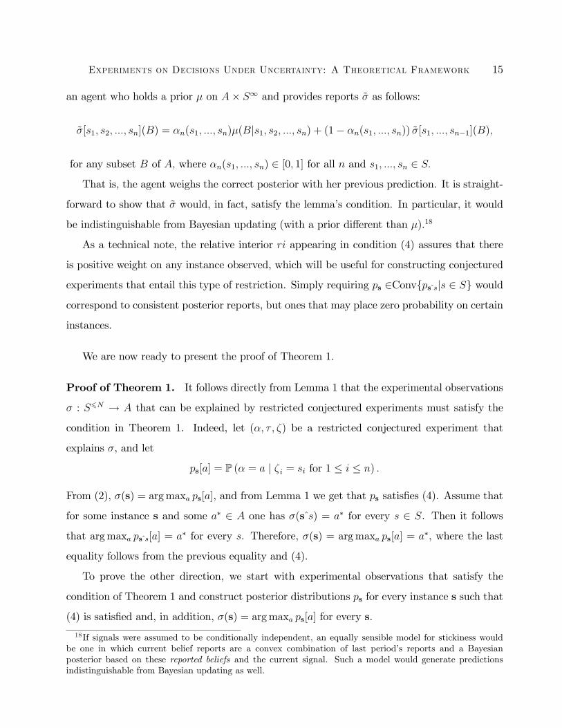
Experiments on Decisions Under Uncertainty: A Theoretical Framework 15
an agent who holds a prior µ on A× S∞ and provides reports σ as follows:
σ[s1, s2, ..., sn](B) = αn(s1, ..., sn)µ(B|s1, s2, ..., sn) + (1− αn(s1, ..., sn)) σ[s1, ..., sn−1](B),
for any subset B of A, where αn(s1, ..., sn) ∈ [0, 1] for all n and s1, ..., sn ∈ S.
That is, the agent weighs the correct posterior with her previous prediction. It is straight-
forward to show that σ would, in fact, satisfy the lemma’s condition. In particular, it would
be indistinguishable from Bayesian updating (with a prior different than µ).18
As a technical note, the relative interior ri appearing in condition (4) assures that there
is positive weight on any instance observed, which will be useful for constructing conjectured
experiments that entail this type of restriction. Simply requiring ps ∈Convps s|s ∈ S would
correspond to consistent posterior reports, but ones that may place zero probability on certain
instances.
We are now ready to present the proof of Theorem 1.
Proof of Theorem 1. It follows directly from Lemma 1 that the experimental observations
σ : S6N → A that can be explained by restricted conjectured experiments must satisfy the
condition in Theorem 1. Indeed, let (α, τ , ζ) be a restricted conjectured experiment that
explains σ, and let
ps[a] = P (α = a | ζ i = si for 1 ≤ i ≤ n) .
From (2), σ(s) = arg maxa ps[a], and from Lemma 1 we get that ps satisfies (4). Assume that
for some instance s and some a∗ ∈ A one has σ(s s) = a∗ for every s ∈ S. Then it follows
that arg maxa ps s[a] = a∗ for every s. Therefore, σ(s) = arg maxa ps[a] = a∗, where the last
equality follows from the previous equality and (4).
To prove the other direction, we start with experimental observations that satisfy the
condition of Theorem 1 and construct posterior distributions ps for every instance s such that
(4) is satisfied and, in addition, σ(s) = arg maxa ps[a] for every s.
18If signals were assumed to be conditionally independent, an equally sensible model for stickiness wouldbe one in which current belief reports are a convex combination of last period’s reports and a Bayesianposterior based on these reported beliefs and the current signal. Such a model would generate predictionsindistinguishable from Bayesian updating as well.

Experiments on Decisions Under Uncertainty: A Theoretical Framework 16
We will use the following additional lemma:
Lemma 2. [One Period Construction] Let∆∗(A) =p ∈ ∆(A)|p[a] < 1
|A|−1 for every a ∈ A
and let p ∈ ∆∗(A). Suppose a1, . . . , am ∈ A are such that either ai 6= aj for some 1 ≤
i, j ≤ m or a1 = · · · = am = arg max p. Then there exists p1, . . . , pm ∈ ∆∗(A) such that
p ∈ ri(Convp1, . . . , pm) and arg max pi = ai.
The proof of Lemma 2 is technical and is deferred to the Appendix. It follows from the
lemma that we can inductively assign posterior probabilities ps ∈ ∆∗(A) for every instance s
such that (4) is satisfied and, in addition,
arg maxaps[a] = σ(a) (5)
for every instance s (indeed, assuming we already defined ps, we define ps S using the lemma,
with m = |S|). By Lemma 1 there exists random variables α, ζ over some probability space
with values in A, SN , respectively, such that ζ has full support and (3) is satisfied. Let τ
be some random variable with values in N, independent of (α, ζ) whose distribution has full
support. Then for every a ∈ A and s = (s1, . . . , sn) ∈ S6N ,
P(α = a | τ = n, ζ1 = s1, . . . , ζn = sn) = P(α = a | ζ1 = s1, . . . , ζn = sn) = ps[a].
By (5) and the last equation it follows that (α, ζ, τ) explains σ, as desired.
Since the proof that the condition in Theorem 1 is necessary was based solely on (2), it
bears on a larger set of conjectures that allow for some correlation between the volume of
information and the realization of signals. Indeed, let us say that a conjectured experiment
(α, τ , ζ) is adapted if τ is measurable with respect to ζ1, . . . , ζn, i.e., if
P(τ = n|α = a, ζ1 = s1, . . . , ζN = sN) = P(τ = n|ζ1 = s1, . . . , ζn = sn),
for every n ∈ N, a ∈ A, and s1, . . . , sN ∈ S (see page 113 in Prokhorov and Shirayev, 1997
for a general definition of adaptable stopping times). This means that when the experimenter
decides whether to continue providing signals after stage n, he can base his decision upon the

Experiments on Decisions Under Uncertainty: A Theoretical Framework 17
already released signals s1, . . . , sn (which were observed by the subject). Importantly, every
restricted conjectured experiment is adapted.
It is easy to verify that (2) is still valid for adapted conjectured experiments. Therefore,
even though the set of adapted conjectured experiments is larger than the set of restricted
conjectured experiments, both sets of conjectured experiments have the same explanatory
power and we get the following corollary:
Corollary 1. [Adapted Conjectured Experiments] If experimental observations can be ex-
plained by an adapted conjectured experiment then they can also be explained by a restricted
conjectured experiment.
In particular, the Corollary implies that allowing subjects to conjecture that the exper-
imenter provides information using a sequential procedure, one in which the experimenter
decides whether or not to provide an additional signal depending on the signals that have
been revealed thus far, leads to the same testable implications described in Theorem 1.
The Sure Thing Principle and Dynamic Consistency. The condition of Theorem 1 is
reminiscent of the “Sure Thing Principle”and the notion of dynamic consistency. Dynamic
consistency suggests that if the decision maker knows that given additional information to-
morrow she will prefer action a to b regardless of what that information will be, then she
should prefer a to b today (see, e.g., Epstein and Le Breton, 1993, Ghirardato, 2002, and ref-
erences therein, as well as Savage, 1954). Note, however, that while the condition in Theorem
1 is expressed solely in terms of the maximal element within the agent’s conditional beliefs,
dynamic consistency is a property of a preference relation over contingent plans. Moreover,
our primitive σ determines only the subject’s action conditioned on a certain class of events,
i.e., events that are given by the assignment of values to certain sets of signals. The condition
of the theorem is therefore weaker than dynamic consistency: if the order induced by observa-
tions σ over actions can be extended to an order over contingent plans that satisfies dynamic
consistency, then σ must satisfy the condition. The Theorem implies that the converse is also
true: if σ satisfies the condition, then it can be explained by Bayesian updating, and therefore
it can be extended to an order over contingent plans that satisfies dynamic consistency. We

Experiments on Decisions Under Uncertainty: A Theoretical Framework 18
emphasize that the suffi ciency part of Theorem 1 cannot be derived from results regarding
dynamic consistency. In fact, without imposing the fixed ordering of signals (thereby allowing
information to be provided via arbitrary sets of signals), the condition of the theorem is not
suffi cient for the observations to be explained by a restricted conjectured experiment. As
mentioned, we provide an analysis of this more general setup in the Online Appendix.
Generating Restricted Conjectures in the Lab. While it is diffi cult to control the
subjective beliefs of subjects in the lab, some experiments are more likely to induce restricted
conjectures by specifying the number of signals subjects will observe at the outset and later
determining both the state and the signals in a transparent manner. We mention two examples
that match our setting particularly well.
The first has to do with the formation of herd behavior in the lab. For instance, in the
classic experiments of Anderson and Holt (1997), the original cascade model of Bikhchandani,
Hirshleifer, and Welch (1992) was tested. In the main treatment, there were six subjects
in each session, one of which was randomly designated as the “monitor” and helped the
experimenters generate the uncertainty and signals in the experiment. In each of 15 periods,
the monitor used a die to determine which of two urns would be used for that period. Urn A
contained two ‘a’balls and one ‘b’ball, and urn B contained two ‘b’balls and one ‘a’ball. Urn
A was used if the throw of the die was one, two, or three; urn B was used otherwise. Subjects
were randomly ordered and each saw one private draw from the selected urn. After seeing
their private draw, each subject had to guess which urn was selected. This guess was then
announced to other subjects. In this way, each subject knew his or her own private draw and
the prior decisions of others, if any, before making a guess. This process continued until all
subjects had made guesses. At the end of each period, the monitor announced which urn had
been selected and each subject was paid $2 if their guess was correct and nothing otherwise.
In this design, the number of signals was determined at the outset and one of the subjects, the
“monitor,”helped assure subjects the experimenters did not release information selectively.
Furthermore, as in our theoretical setting, it was in the best interest of the subjects to report
the alternative, which urn had been selected, they thought was more likely.19
19The use of subjects as “monitors”may be a useful way to restrict subjects’conjectures and appears in

Experiments on Decisions Under Uncertainty: A Theoretical Framework 19
The results suggested about half as many reverse cascades as there were normal cascades
that theory predicts with Bayesian updating based on the underlying uncertainty and equi-
librium behavior. The authors suggested a model of errors, which is consistent with subjects
relying more on their own private information. However, they also noted that about a third
of their subjects seem to rely on a simple count of signals, which is consistent with Bayesian
updating with a different information generation process (e.g., one in which each preceding
subject’s guess reflects their private draw and is not impacted by previous guesses).
The second example of an experiment that fits our restricted conjectures setting is provided
by the recent work of Mobius et al. (2014), who look at the evolution of subjects’beliefs about
being among the top half of performers in an IQ quiz. At the outset, subjects responded to
an IQ quiz. Their beliefs about being among the top half of performers were elicited after the
quiz. There were then four stages, which were announced at the outset. At each stage, each
subject initially received a binary signal that indicated whether the subject was among the
top half of performers; that signal was correct with 75% probability. Subjects then reported
their belief about being among the top half of performers. That is, subjects received four
conditionally independent signals that depended on their own performance and others’. Since
both the realized state and the signals were generated by the subjects themselves, this design
was likely to induce restricted conjectures.
The results illustrate that subjects over-weigh positive feedback relative to negative feed-
back and are conservative —they have sticky beliefs in that they update too little in response
to both positive and negative feedback. The authors suggest, in line with our results, that sub-
jects update as if they misinterpret signal distributions in a self-serving manner, but process
these modified signals using Bayes’rule.
We now turn to analyze the testable implications derived when conjectured experiments
are fully unrestricted.
several other experimental designs. For another experiment in the context of Bayesian updating, see El-Gamaland Grether (1995).
Experiments on Decisions Under Uncertainty: A Theoretical Framework 20
4. Unrestricted Conjectured Experiments
When conjectured experiments are unrestricted, the amount of information observed can be
perceived as correlated with the realization of uncertainty. The requirement appearing in
Theorem 1 is then too strong. As an example, consider the classical experiment of Tversky
and Kahneman (1983). In their experiment, subjects were told that “Linda is 31 years old,
single, outspoken, and very bright. She majored in philosophy. As a student, she was deeply
concerned with issues of discrimination and social justice, and also participated in anti-nuclear
demonstrations.”Subjects were then asked to determine which is more likely: 1. Linda is a
bank teller; or 2. Linda is a bank teller and is active in the feminist movement. 85% of the
subjects chose the second option. This was taken as evidence for the failure of conjunction
of probabilities. However, a different interpretation is that the mere fact the experimenter
chose to expose Linda’s participation in demonstrations suggests that 2 is the appropriate
answer. In other words, the information revealed (captured by the details appearing in the
blurb describing Linda) could be perceived to be correlated with the underlying state (which
answer the experimenter expects). In fact, many experiments falling under the general rubric
of the Representative Heuristic (see Tversky and Kahneman, 1974) have this feature of a
scenario, or a person’s profile, that is described in some detail and followed by a classification
query.
The following is an example in the same spirit utilizing our notation.
Example 1. [Explanatory Power of Unrestricted Conjectures] Assume that N = 1, S =
u, d, A = a, b, and consider the experimental observations σ given by:
σ(e) = a and σ(u) = σ(d) = b,
as depicted in tree form in Figure 1, Panel (3). Note that the condition of Theorem 1 is
not satisfied, and therefore σ cannot be explained by a restricted conjectured experiment.
However, σ can be explained by an unrestricted conjectured experiment (α, τ , ζ) such that τ
and ζ are independent conditional on the realized alternative α and, in addition, characterized

Experiments on Decisions Under Uncertainty: A Theoretical Framework 21
by the following:
P(α = a) = P(α = b) =1
2
P(τ = 0|α = a) = 1− P(τ = 1|α = a) = 0.9
P(τ = 0|α = b) = 1− P(τ = 1|α = b) = 0.1
P(ζ = u | α = a) = P(ζ = d | α = a) = 0.5 for every a ∈ a, b.
As explained in the paper’s introductory example, the conjectured experiment is such
that when the realized alternative is α = a, the subject perceives receiving no signals as
extremely likely, whereas when the realized alternative is α = b, the subject perceives receiving
a signal as very likely. However, the determination of the number of signals observed is done
independently of the generation of the signals themselves. In fact, the signals in and of
themselves are uninformative.
It turns out that any experimental observations can be explained with an unrestricted
conjectured experiment, formally captured in the following “anything goes”result:
Theorem 2. [Unrestricted Conjectured Experiments] For every σ : S6N → A the experi-
mental observations σ admit an explanation by an unrestricted conjectured experiment.
From the theorem, when subjects’ conjectures are unconstrained, anomalous updating
behavior is indistinguishable from particular framing of the experimental design itself.
The proof of Theorem 2, as the proof of Theorem 1, follows two steps. We first show that
any set of posteriors can be explained with an unrestricted conjectured experiment. This is
the crucial step in the proof, since it is then immediate to choose a sequence of posteriors
that is consistent with the observations, and therefore rationalizes them with an unrestricted
conjecture. Formally, the analogue of Lemma 1 is the following:
Lemma 3. [Explainable Posteriors —Unrestricted] Let ps ∈ ∆(A) be an assignment of prob-
ability distribution over A for every instance s ∈ S6N . Then there exist random variables
(α, τ , ζ) over some probability space (Ω,A,P), with values in A,N, SN respectively, such that

Experiments on Decisions Under Uncertainty: A Theoretical Framework 22
1. for every n ∈ N and every s1, . . . , sn ∈ S,
P(τ = n, ζ i = si for 1 ≤ i ≤ n) > 0;
2. For every instance s = (s1, . . . , sn) and every a ∈ A
P (α = a | τ = n, ζ i = si for 1 ≤ i ≤ n) = ps[a]. (6)
The lemma is conceptually important in that it highlights how robust the message of The-
orem 2 is to what is elicited by the experimenter when subjects’conjectures are unrestricted.
Indeed, even if for each instance the full belief were elicited (instead of the most likely state),
Lemma 3 assures that an analogous “anything goes”result would still hold and any experi-
mental observations (now entailing posterior beliefs for all instances) could be explained with
an unrestricted conjecture.
The proof of Lemma 3, appearing in the Appendix, is at the root of our “anything goes”
result. Intuitively, an unrestricted conjectured experiment ultimately corresponds to a joint
distribution µ over A×N×SN . For any assignment of posteriors pss∈S6N , ps ∈ ∆(A), pick
an arbitrary distribution ν over N× SN and define µ as:
µ(k, n, s1, ..., sN) = ν (n, s1, ..., sN) p(s1,...,sN ) [a] .
Then, the conditional distribution of µ given the number of signals n and full realization
(s1, ..., sN) is p(s1,...,sN ). It follows that the conditional distribution of µ given n and (s1, ..., sn)
is ps, where s = (s1, ..., sn) , as required. The proof of Theorem 2 now follows immediately:
Proof of Theorem 2. For experimental observations σ : S6N → A we choose arbitrarily, for
every instance s ∈ S6N , a probability distribution ps ∈ ∆(A) such that arg maxa ps[a] = σ(s).
The corresponding random variables α, τ , and ζ, whose existence is asserted in Lemma 3,
explain σ.
Aggregate Data. Theorems 1 and 2 pin down the testable implications of restricted and
unrestricted conjectured experiments when we observe the response of a single subject after

Experiments on Decisions Under Uncertainty: A Theoretical Framework 23
every sequence of signals. In practice, experimenters usually work with aggregate data from
responses of a random sample of subjects, each of whom has responded only to some sequences
of signals.
Suppose each subject is asked to make a decision after a single signal sequence s. Theorem
1 can be used to deduce the testable implications of such data, assuming the hypotheti-
cal (unobserved) responses of every subject are rationalized by some conjectured experiment
(though not necessarily the same conjecture for every subject). In the Online Appendix we
provide a detailed model of such a setting. Here, assume, for example, that A = a, b and
S = u, d and, for every sequence s of signals, let θ(s) be the proportion of subjects who
pick a when provided with the signal sequence s. Assume further that each of these subjects
respond to the experimental queries using a function σ : S6N → A that can be rational-
ized by some restricted conjectured experiment (i.e., satisfies the condition of Theorem 1).
Then, it must be the case that θ(s) 6 θ(sˆu) + θ(sˆd) 6 θ(s) + 1 for every s ∈ SN . Indeed,
θ(s) ≤ θ(sˆu) + θ(sˆd) since every subject who chooses a after s must be either among the
subjects who would choose a after sˆu or among the subjects who would choose a after sˆd.
Similarly, 1− θ(s) ≤ (1− θ(sˆu)) + (1− θ(sˆd)) (or, equivalently, θ(sˆu) + θ(sˆd) ≤ θ(s) + 1)
since every subject who chooses b after s must be either among the subjects who would choose
b after sˆu or among the subjects who would choose b after sˆd.
We can estimate θ(s) from the sample. Statistically significant violations of this inequality
will therefore refute the hypothesis that subjects respond according to some restricted con-
jectured experiment. On the other hand, it follows from Theorem 2 that every distribution of
subjects’responses can be rationalized as the aggregation of responses of subjects associated
with some unrestricted conjectured experiment.
To summarize our results up to now, we have characterized the testable implications of
Bayesian updating for two polar cases pertaining to subjects’ freedom regarding the fram-
ing of the experimental design. When conjectures are fully restricted, standard updating is
equivalent to a type of dynamic consistency condition. When conjectures are unrestricted,
standard updating has no testable implications. In what follows, we analyze testable implica-
tions derived from intermediate restrictions.

Experiments on Decisions Under Uncertainty: A Theoretical Framework 24
5. Partially Restricted Conjectured Experiments
In this section, we consider intermediate restrictions that may correspond to experimental
designs in which signals (but not states) are determined in the lab in front of the subjects
(and the number of signals is a design choice). Indeed, many of the recent social learning
and voting experiments follow protocols of this nature. In these experiments, two uncertain
alternatives are often manifested in two jars that contain a majority of either, say, red or blue
balls. Subjects, not knowing which jar had been selected can then draw a pre-determined
number of balls, often with replacement, from the chosen jar and observe their color20 (for a
survey of such experiments, see Palfrey, 2006, 2013).
With such designs, it is natural to assume the subject believes the number of signals she
receives is uncorrelated with the realizations of the signals (but may be correlated with the
realized alternative). We formalize such conjectures as follows:
Definition 4. [Partially Restricted Conjectured Experiment] A partially restricted conjec-
tured experiment is a conjectured experiment (α, τ , ζ) such that τ and ζ are conditionally
independent given α, i.e.,
P(τ = n, ζ = x|α = a) = P(τ = n|α = a) · P(ζ = x|α = a),
for every n ∈ N, x ∈ SN , and a ∈ A.
We assume hereafter a binary state space, A = a, b.21 Note that the conjecture proposed
in Example 1 is partially restricted and so that example illustrates that the explanatory power
of partially restricted conjectured experiments is larger than that of restricted conjectured
experiments. However, not all experimental observations can be explained by a partially
restricted conjectured experiment, as illustrated by the following example, formalizing the
example we discussed in our introduction:
20Our framework encompasses such strategic interactions since we can always rename the alternatives ap-propriately. Namely, in strategic interaction experiments, subjects select the action (which serves as ouralternative) that is more likely to deliver higher payoffs.21Our characterization in this section relies on techniques tailored for a binary set of alternatives. While
many experiments satisfy this restriction (for instance, much of the experimental literature on voting focuseson binary elections), we view the extension to richer sets of alternatives as an interesting direction for futureresearch.

Experiments on Decisions Under Uncertainty: A Theoretical Framework 25
Example 2. [Unexplainable Reversals] Assume that N = 2, S = u, d and consider the
experimental observations σ depicted in Figure 2. Let s and t be the signal sequences (u) and
(d) respectively (so d(s) = d(t) = 1). On the one hand, controlling for any learning from the
sheer amount of information released, s is more supportive of the alternative a than t (from
the subject’s point of view) since σ(s) = a and σ(t) = b. On the other hand, the same can
be said in reverse, since conditioning on depth 2 of the tree, σ(s s) = b and σ(t t) = a for
every s, t ∈ u, d. This inconsistency implies that the experimental observations cannot be
explained by a partially restricted conjectured experiment.
Examples 1 and 2 illustrate that the explanatory power of partially restricted conjectured
experiments is strictly between that of unrestricted and restricted conjectured experiments.
Our characterization of the class of observations that are explainable with partially re-
stricted conjectures entails ruling out a generalized set of reversals of the type appearing
in Example 2. Roughly speaking, reversals that are consistent with Bayesian updating are
described by “tending to a specific report”for a particular length of signal sequence.
Formally, fix experimental observations σ. For a pair of instances s, t of the same depth
we define recursively what we mean by “the conditional probability of state ‘a’given s is
behaviorally revealed higher than the conditional probability of state ‘a’given t,”where the
conditioning is on the value of signals received, but not their number. We say shortly that s
is revealed higher than t.22
Definition 5. [Revealed Higher Relation] Let σ : S6N → a, b be experimental observa-
tions. For a pair of instances s, t ∈ S6N of the same depth the relation ‘s is revealed higher
than t under σ’is recursively defined using the following rules:
1. If σ(s) = a and σ(t) = b, then s is revealed higher than t.
2. If s s is revealed higher than t t for every s, t ∈ S, then s is revealed higher than t.
The following lemma illustrates the implication of one instance being revealed higher than
another in terms of probabilistic assessments.
22Note that “revealed higher”need not be a complete relation, nor is it necessarily anti-symmetric.

Experiments on Decisions Under Uncertainty: A Theoretical Framework 26
Lemma 4. [Revealed Higher —Probabilities] Let σ : S6N → a, b be experimental obser-
vations, and let (α, τ , ζ) be a partially restricted conjectured experiment that explains σ. If
s = (s1, . . . , sn) and t = (t1, . . . , tn) ∈ S6N are a pair of instances such that s is revealed
higher than t under σ, then
P(α = a|ζ1 = s1, . . . , ζn = sn) > P(α = a|ζ1 = t1, . . . , ζn = tn).
Lemma 4 assures that if the experimental observations can be explained by a partially
restricted conjectured experiment, it cannot be the case that there are reversals of the form s
is revealed higher than t and t is revealed higher than s for some instances s and t. As it turns
out, the reverse is also true. Indeed, the following theorem characterizes the set of experimental
observations that can be explained by a partially restricted conjectured experiment.
Theorem 3. [Partially Restricted Conjectured Experiments] The experimental observations
σ : S6N → a, b can be explained by a partially restricted conjectured experiment if and only
if the order revealed higher is anti-symmetric. That is, there exists no pair s, t of instances
such that s is revealed higher than t and t is revealed higher than s.
The formal proof of the suffi ciency of the condition is intricate and appears in the Online
Appendix, together with the formal proof of Lemma 4.
In order to provide the reader with some intuition, we provide here a sketch of the proof
of the theorem. Assume that the experimental observations σ : S6N → a, b satisfy the
theorem’s condition. We construct the partially restricted conjectured experiment (α, τ , ζ)
that explains σ in two steps. First, we construct random variables (α, ζ) such that
P(α = a|ζ1 = s1, . . . , ζn = sn) > P(α = a|ζ1 = t1, . . . , ζn = tn).
for every pair s = (s1, . . . , sn) and t = (t1, . . . , tn) of instances of the same length such that
σ(s) = a and σ(t) = b. In the second step, we add a random variable τ that is independent
of ζ given α and, for every n, we choose the probabilities P(α = a|τ = n) so that
P(α = a|τ = n, ζ1 = s1, . . . , ζn = sn) > 1/2

Experiments on Decisions Under Uncertainty: A Theoretical Framework 27
for all instances s = (s1, . . . , sn) such that σ(s) = a and
P(α = a|τ = n, ζ1 = t1, . . . , ζn = tn) < 1/2
for all instances t = (t1, . . . , tn) such that σ(t) = b.
In words, we first construct conjectures that are consistent within each layer of the tree
of observations (that is, for a fixed number of signals). We then construct the correlation
between the number of signals observed and underlying state so that the assessments across
layers are consistent.
The main diffi culty is in the first stage. The proof makes use of the tree structure over
the set of instances. For every instance s = (s1, . . . , sn) ∈ S6N we assign a number ps ∈ [0, 1]
such that ps ∈ ri(Convps s|s ∈ S) and ps > pt whenever s, t are two instances of the same
length and s is revealed higher than t. Then, by Lemma 1 we can construct random variables
α, ζ such that
ps = P(α = a|τ = n, ζ1 = s1, . . . , ζn = sn)
for every instance s = (s1, . . . , sn).
We assign the numbers ps to nodes s by induction over the depth of s, working from the
root of the tree to the leafs. Assume that we have already defined the values ps for nodes of
depth n − 1 and consider now the set X of nodes of depth n. The relation revealed higher
induces a partial order over X, which we denote by ≤. In addition, there is a natural partition
A over the set X, whose atoms are the set of instances with a common source in the tree.
Thus, the atoms of A correspond to nodes of depth n − 1. Since we have already defined ps
over these nodes, we need to “lift”p to a function over X that is monotone with respect to
≤. Much of the technical aspects of the proof are dedicated to showing that this is indeed
possible, using the fact that the order “revealed higher”is an interval order.23
We note that Theorem 3 gives rise to a simple algorithm for checking whether experimental
observations in a finite tree can be explained by a partially restricted conjectured experiment:
Go over all the layers of the tree of instances, from the layer of depth d = N to the layer of
23In terms of technical generality, we note that Theorems 1, 2, and 3 all easily extend to environments inwhich the number of signals is not bounded.

Experiments on Decisions Under Uncertainty: A Theoretical Framework 28
Figure 3: Algorithmically Checking Consistency
depth d = 0 (i.e., from the leafs to the root of the corresponding tree). For every layer d,
construct the relation “s is higher than t”for instances s, t of that layer (using Definition 5
and the already constructed relation over layer d+ 1) and check that the condition is satisfied
over nodes in that layer. Using this algorithm, the reader can verify that the experimental
observation in the following example cannot be explained by a partially restricted conjectured
experiment.
Example 3. [Explainability Algorithm] Consider the Example depicted in Figure 3 (notation
following that of our previous examples). Note that (u) is revealed higher than (d) . However,
algorithmically proceeding from the leafs to layer 1 we see that, from layer 3, (d, u) and
(d, d) are revealed higher than (u, u), and from layer 2, (d, u) and (d, d) are also revealed
higher than (u,d), which therefore implies that (d) is revealed higher than (u) . In particular,
the condition of Theorem 3 is not satisfied and these observations cannot be explained by a
partially restricted conjectured experiment.
Example 3 also demonstrates that lack of “simple reversals”of the type of Example 2 is
not suffi cient for experimental observations to admit an explanation by a partially restricted
conjectured experiment.

Experiments on Decisions Under Uncertainty: A Theoretical Framework 29
6. Conclusions
This paper provides a theoretical framework for analyzing experimental data accounting for
subjects’conjectures regarding the experimental design itself. When subjects’conjectures are
unrestricted, we illustrate an “anything goes” result: any experimental observations can be
explained with standard updating and the appropriate choice of a conjectured experiment (in
fact, generically, multiple conjectured experiments would explain the observations). When
subjects’conjectures are restricted, in terms of the perceived correlation between the amount
of information revealed to them in the lab and the underlying realized uncertainty, our results
provide a full characterization of the testable implications standard updating entails. To
the extent that experimental transparency (say, regarding the way information is generated
in the lab) yields more restricted conjectures, the overwhelming message from our results
is that transparency is crucial for meaningful testable implications of theoretical predictions
pertaining to decision making under uncertainty.
A. Appendix
A.1. Restricted Conjectured Experiments.
Proof of Lemma 1. Let α, ζ be random variables that satisfy the condition of the Lemma.Then, for every n < N and every s = (s1, . . . , sn) ∈ Sn it follows from condition 2 and thelaw of total probability that
ps[a] = P (α = a | ζ i = si for 1 ≤ i ≤ n) =∑s∈S
P(ζn+1 = s | ζ i = si for 1 ≤ i ≤ n
)·P(α = a | ζ i = si for 1 ≤ i ≤ n, ζn+1 = s
)=∑s∈S
λspss[a],
where λs = P(ζn+1 = s | ζ i = si for 1 ≤ i ≤ n
)> 0 by condition 1. Therefore, ps ∈ ri(Convps s|s ∈
S) as desired.Assume now that for every s = (s1, . . . , sn) one has ps ∈ ri(Convps s|s ∈ S), so that
ps =∑s∈S
λs,spss. (7)
for some λs,s > 0 such that∑
s λs,s = 1. Let ζ1, . . . , ζn, α be random variables such that
P(ζn+1 = s | ζ1 = s1, . . . , ζn = sn
)= λs,s (8)

Experiments on Decisions Under Uncertainty: A Theoretical Framework 30
for every n < N , s = (s1, . . . , sn), s ∈ S, and
P (α = a | ζ1 = s1, . . . , ζN = sN) = ps[a] (9)
for every s = (s1, . . . , sN). Since λs,s > 0, it follows from (8) that
P (ζ1 = s1, . . . , ζN = sN) = Πn<NP(ζn+1 = sn+1 | ζ1 = s1, . . . , ζn = sn
)> 0,
so that the first condition in Lemma 1 is satisfied. We now prove the second conditionby backward induction over n. For n = N the condition follows from (9). Let n < N ,s = (s1, . . . , sn) ∈ S, and assume the condition is true for n+ 1. Then,
P (α = a|ζ i = si for 1 ≤ i ≤ n) ==∑
s P(ζn+1 = s | ζ i = si for 1 ≤ i ≤ n
)· P (α = a|ζ i = si for 1 ≤ i ≤ n+ 1) =
=∑
s λs,spss[a] = ps[a],
where the first equality follows from the law of total probability, the second from (8) and theinduction hypothesis, and the third from (7). Proof of Lemma 2. If a1 = · · · = am = arg max p then we can choose pi = p for 1 ≤ i ≤ m.Assume now that a1 6= a2. We choose p3, . . . , pm ∈ ∆∗(A) arbitrarily such that arg maxa pi[a] =
ai. Let ε > 0 be suffi ciently small so that (m− 2)ε < 1 and p′ ∈ ∆∗(A), where
p′ =1
1− (m− 2)ε(p− ε(p3 + · · ·+ pm)) . (10)
The existence of such ε follows from the fact that ∆∗(A) is an open set and the right handside of (10) converges to p ∈ ∆∗(A) as ε goes to 0.We now define p1 and p2. Choose q such that
maxap[a] < q <
1
|A| − 1, (11)
and let r = 1 −∑
a6=a1,a2 p′[a] − q. Note that from the fact that p′[a] < 1
|A|−1 for every a ∈ Aand q < 1
|A|−1 it follows that r > 0. Moreover, since q > p′[a1] it follows that
r = 1−∑
a6=a1,a2
p′[a]− q < 1−∑a6=a2
p′[a] = p′[a2] < q <1
|A| − 1. (12)
For i = 1, 2 and j = 3− i, let
pi[a] = p′[a] for a 6= a1, a2 (13)
pi[ai] = q (14)
pi[aj] = r. (15)
Then, it follows from (12) that pi ∈ ∆∗(A) and arg maxa pi[a] = ai.

Experiments on Decisions Under Uncertainty: A Theoretical Framework 31
In addition, it follows from (11) and (12) that r < p′[a2] < q. Therefore,
p′[a2] = λr + (1− λ)q (16)
for some 0 < λ < 1. We claim that
p′ = λp1 + (1− λ)p2 (17)
i.e., p′[a] = λp1[a] + (1− λ)p2[a] for every a ∈ A. (18)
Indeed, for a 6= a1, a2, the equality follows from the fact that, by (13), p1[a] = p2[a] = p′[a].For a = a2, the equality follows from (14),(15), and (16). For a = a1, the equality followsfrom the equality in all other coordinates and the fact that both sides of (18) sum to 1 (overa ∈ A). Finally, it follows from (10) and (17) that
p = (1− (m− 2)ε) p′ + ε(p3 + · · ·+ pm) = λ1p1 + λ2p2 + λ3p3 + · · ·+ λmpm,
where
λ1 = (1− (m− 2)ε) · λ,λ2 = (1− (m− 2)ε) · (1− λ), and
λ3 = · · · = λm = ε.
.
Therefore, p ∈ ri(Convp1, . . . , pm), as desired.
A.2. Unrestricted Conjectured Experiments.
Proof of Lemma 3. Choose arbitrarily a distribution ν over N × SN with full support.Let α, τ , ζ be random variables over some probability space (Ω,A,P) with values in A,N, SN
such that:
1. The joint distribution of τ and ζ is ν.
2. The conditional distribution of α given τ = n and ζ = x is ps, where s = x|n:
P (α = a|τ = n, ζ = x) = ps[a] (19)
We proceed to prove that (6) is satisfied for every instance s = (s1, . . . , sn). The eventτ = n, ζ i = si for every 1 ≤ i ≤ n is the disjoint union of the events τ = n, ζ = x,ranging over all x ∈ SN such that x|n = s. Therefore, by the law of total probability,
P (α = a | τ = n, ζ i = si ∀1 ≤ i ≤ n) =∑x∈SN and x|n=s
P (ζ = x|τ = n, ζ i = si ∀1 ≤ i ≤ n)P (α = a|τ = n, ζ = x) = ps[a],
where the last equality follows from (19).

Experiments on Decisions Under Uncertainty: A Theoretical Framework 32
References
Lisa R. Anderson and Charles A. Holt (1997), “Information Cascades in the Laboratory,”American Economic Review, 87(5), 847-862.
Francis J. Anscombe and Robert .J. Aumann (1963), “A Definition of Subjective Probability,”Annals of Mathematical Statistics, 34, 199-205.
Henry K. Beecher (1955) “The powerful placebo,”Journal of the American Medical Association,159, 1602-1606.
Roland Benabou and Jean Tirole (2002), “Self-Confidence and Personal Motivation.”QuarterlyJournal of Economics, 117(3), 871—915.
Sushil Bikhchandani, David Hirshleifer, and Ivo Welch (1992), “A Theory of Fads, Fashion,Custom, and Cultural Change as Informational Cascades,” Journal of Political Economy, 100(5),992-1026.
Kim C. Border (2003), Alternative Linear Inequalities.Isabelle Brocas and Juan D. Carrillo (2003), The Psychology of Economic Decisions, Volume 1,
Rationality and Well-Being, Oxford University Press: Oxford, UK.Isabelle Brocas and Juan D. Carrillo (2004), The Psychology of Economic Decisions, Volume 2,
Reasons and Choices, Oxford University Press: Oxford, UK.Colin F. Camerer, George Loewenstein, and Matthew Rabin (Eds.) (2006), Advances in Behav-
ioral Economics, Princeton University Press.Olivier Compte and Andrew Postlewaite (2004), “Confidence-Enhanced Performance,”American
Economic Review, 94(5), 1536-1557.Larry G. Epstein and Michel Le Breton (1993), “Dynamically Consistent Beliefs Must be Bayesian,”
Journal of Economic Theory, 61(1), 1-22.Mahmoud El-Gamal and David Grether (1995), “Are People Bayesian? Uncovering Behavioral
Strategies,”Journal of the American Statistical Association, 90(432), 1137-1145.Peter C. Fishburn (1985), Interval Orders and Interval Graphs: A Study of Partially Ordered
Sets, Wiley.Daniel Friedman and Shuyam Sunder (1994), Experimental Methods: A Primer for Economists,
Cambridge University Press.Paolo Ghirardato (2002), “Revisiting Savage in a Conditional World ,”Economic Theory, 20(1),
83-92.Itzhak Gilboa and David Schmeidler (1993), “Updating Ambiguous Beliefs,”Journal of Economic
Theory, 59, 33-49.Richard Gillespie (1991), Manufacturing Knowledge: A History of the Hawthorne Experiments,
Cambridge: Cambridge University Press.Edward J. Green and In-Uck Park (1996), “Bayes Contingent Plans,”Journal of Economic Be-
havior and Organizations, 31, 225-236.John H. Kagel and Alvin E. Roth (1997), The Handbook of Experimental Economics, Princeton
University Press.Daniel Kahneman, Paul Slovic, and Amos Tversky (1982), Judgment under Uncertainty: Heuris-
tics and Biases, Cambridge University Press.Botond Koszegi (2006), “Ego Utility, Overconfidence, and Task Choice,”Journal of the European
Economic Association, 4(4), 673-707.

Experiments on Decisions Under Uncertainty: A Theoretical Framework 33
Markus Mobius, Muriel Niederle, Paul Niehaus, and Tanya S. Rosenblat (2014), “ManagingSelf-Confidence,”mimeo.
Richard E. Nisbett and Lee Ross (1980), Human inference: Strategies and shortcomings of socialjudgement. Englewood Cliffs: Prentice-Hall, Inc.
Delroy L. Paulhus (1991) “Measurement and control of response bias,” In J.P. Robinson, P.R.Shaver, and L.S. Wrightsman, (Eds.), Measures of Personality and Social Psychological Attitudes,San Diego: Academic Press.
Thomas R. Palfrey (2006), “Laboratory Experiments in Political Economy,” in Handbook ofPolitical Economy, B. Weingast and D. Wittman eds. Oxford University Press: Oxford.
Thomas R. Palfrey (2013), “Experiments in Political Economy,” in The Handbook of Experi-mental Economics, Volume II, J. Kagel and A. Roth eds., forthcoming.
Yurij V. Prokhorov and Albert N. Shiryaev (1997), Probability Theory III: Stochastic Calculus(Encyclopaedia of Mathematical Sciences), Springer.
Matthew Rabin and Joel L. Schrag (1999), “First Impressions Matter: A Model of ConfirmatoryBias,”Quarterly Journal of Economics, 114(1), 37-82.
Leonard J. Savage (1954), The Foundations of Statistics, Wiley.Reinhard Selten (1967), “Die Strategiemethode zur Erforschung des eingeschränkt rationalen
Verhaltens im Rahmen eines Oligopolexperiments”(translated to “The Strategy Method for Researchon Boundedly Rational Behavior in the Context of an Oligopoly Experiment”), in: Beiträge zurExperimentellen Wirtschaftsforschung, H. Sauermann, ed., 136-168.
Shelley E. Taylor and Jonathan D. Brown (1988), “Illusion and Well-Being: A Social Psycholog-ical Perspective on Mental Health.”Psychological Bulletin, 103(3), 193-210.
Amos Tversky and Daniel Kahneman (1974), “Judgement Under Uncertainty: Heuristics andBiases,”Science, 185(4157), 1124-1131.
Amos Tversky and Daniel Kahneman (1983), “Extension versus intuitive reasoning: The con-junction fallacy in probability judgment,”Psychological Review, 90 (4), 293-315.
Amos Tversky and Eldar Shafir (1992), “The disjunction effect in choice under uncertainty,”Psychological Science, 3, 305-309.
Jonathan Weinstein (2013), “A Bayesian Foundation for Classical Hypothesis Testing,”mimeo.Leeat Yariv (2005), “I’ll See It when I Believe It,”mimeo.Daniel J. Zizzo (2010), “Experimenter Demand Effects in Economic Experiments,”Experimental
Economics, 13(1), 75-98.
Recommended