EFFECT OF EXCHANGE RATE FLUCTUATIONS AND OIL PRICE SHOCKS: THE NIGERIAN EXPERIENCE, 1986 – 2008.
A
Ph.D THESIS
BY
UGWUANYI, CHARLES UCHE (PG/Ph.D/03/34674)
DEPARTMENT OF ECONOMICS UNIVERSITY OF NIGERIA, NSUKKA
i
TITLE PAGE
EFFECT OF EXCHANGE RATE FLUCTUATIONS AND OIL PRICE SHOCKS: THE NIGERIAN EXPERIENCE, 1986 – 2008.
BY
UGWUANYI, CHARLES UCHE (PG/Ph.D/03/34674)
THESIS SUBMITTED IN FULFILLMENT OF THE REQUIREMENTS FOR THE DEGREE OF DOCTOR OF PHILOSOPHY,
DEPARTMENT OF ECONOMICS, UNIVERSITY OF NIGERIA, NSUKKA.
JUNE, 2011
ii
APPROVAL
___________ __________ PROF. F.E. ONAH SIGNATURE DATE (SUPERVISOR) PROF. S.I. UDABA ____________ __________ (EXTERNAL EXAMINER) SIGNATURE DATE ____________________ _____________ __________ (INTERNAL EXAMINER) SIGNATURE DATE _____________ __________ PROF. C.C. AGU SIGNATURE DATE (HEAD OF DEPARTMENT) PROF. E.O. EZEANI ______________ __________ (DEAN OF THE FACULTY) SIGNATURE DATE

1
DEDICATION
TO THE ALMIGHTY GOD AND ALL ERUDITE
iii

2
ACKNOWLEDGEMENT
My sincere and profound gratitude goes to my supervisor Prof. F.E.
Onah in particular and in general to all the academic and non academic
staff of Department of Economics, University of Nigeria, Nsukka for their
unquantifiable contributions in my educational pursuit.
I am highly indebted to Dr. F.O. Asogwa for his painstaking
assistance and constructive criticisms to the work.
I equally recognize my ebullient professors of Economics; Professors
C.C. Agu (Head Department of Economics UNN), N.I. Ikpeze, O.E. Obinna,
Ukwu I. Ukwu and Dr. (Mrs.) Gladys Aneke whose words of advice and
encouragement put me through to this stage.
I also owe a lot of thanks to Dr. P.C. Omoke Messrs I.O. Agwu, N.U.
Onwukwe, Thom. Okoro, D. Nnachi, G.E. Onwe, C.C. Udude and other
colleagues in the Department of Economics, Ebonyi State University,
Abakaliki.
Also, special to be mentioned are E.R. Ukwueze, Joseph Nnadi, Jude
Chukwu, S.E. Ugwuanyi, Prof. O.S. Abonyi, Dr. E.S. Obe, Dr. B.M. Mba,
Dr. Boniface Ugwuishiwu, Dr. Oscar. O. Eze, Dr. O.C. Eze, S.G.
Edoumiekumo and a host of other friends and relations for their support. I
remain grateful.
iv

3
I am equally grateful to my computer operator Miss Chizoba
Ugwuoke for her dedication to the job.
My thanks equally go to Mrs. Veronica Ugwuanyi (Nee Agbowo) the
woman through whom I came to be), my wife Caroline Ugwuanyi and my
children Amuche, Chibueze, Ebuka, Elendu and Nchetachukwu for being
behind me through out the studies.
Above all, I remain grateful to Almighty God for giving me life and
good health.
Charles Uche Ugwuanyi
v
4
LIST OF TABLES
Table 1: Summary of Related Empirical Literature - - 54
Table 5.1 Unit Root Test at Level Forms - - - - 54
Table 5.2 Unit Root Test at 1st Difference - - - - 55
Table 5.3 Johansen‟s Co-Intergration Test - - - - 59
Table 5.4 Johansen‟s Co-Integration Test Summary - - 60
Table 5.5 Johansen‟s Co-Integration Test Between REF and OPF 61
Table 5.6 Real Exchange Rate (RER) - - - - - 62
Table 5.7 Oil Price (OIP) - - - - - - - 63
Table 5.8 Index of Industrial Production (IIP) - - - 65
Table 5.9 Industrial Production Growth Rate (IPR) - - 66
Table 5.10 Degree of Trade Openness (TRO) - - - 67
Table 5.11 Real Exchange Rate D (RER) - - - - 69
Table 5.12 Oil Price D (OIP) - - - - - - 70
Table 5.13 Real Exchange Rate Fluctuations D (REF) - - 71
Table 5.14 Oil Price Fluctuation D (OPF) - - - - 72
Table 5.15 Index of Industrial Production D (IIP) - - - 73
Table 5.16 Industrial Production Growth Rate D (IPR) - - 74
Table 5.17 Degree of Trade Openness D (TRO) - - - 75
Table 5.18 Result of GARCH Variance (REF as Dependent Variable) 76
vi

5
Table 5.19 Result of GARCH Variance (OPF as Dependent Variable) 76
Table 5.20 Result of EGARCH Model (RER as Dependent Variable) 77
Table 5.21 Variance Equation for OIP - - - - - 78
vii
6
LIST OF FIGURES
Figure 5A: Real Exchange Rate and Oil Price - - 57
Figure 5B: Oil Price Fluctuations and Real Exchange Rate
Fluctuations - - - - - - 58
Figure 5C: Graph of GARCH Variance of RER and OIP - 79
viii
7
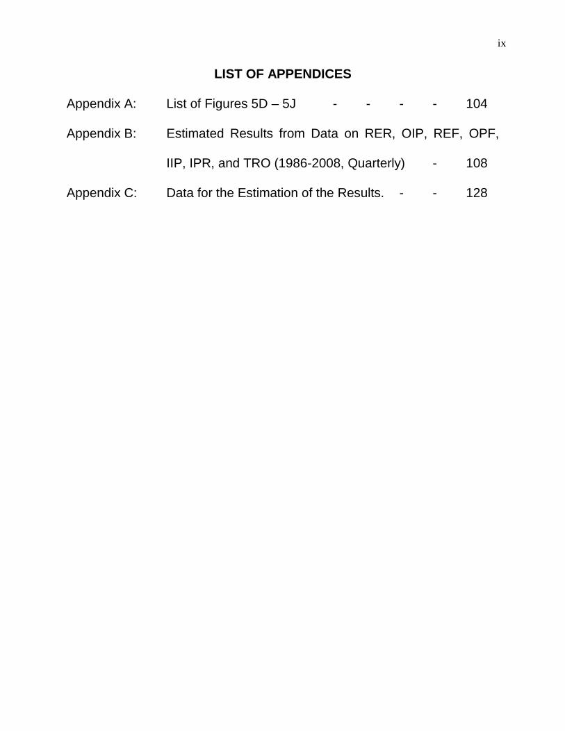
LIST OF APPENDICES
Appendix A: List of Figures 5D – 5J - - - - 104
Appendix B: Estimated Results from Data on RER, OIP, REF, OPF,
IIP, IPR, and TRO (1986-2008, Quarterly) - 108
Appendix C: Data for the Estimation of the Results. - - 128
ix
8
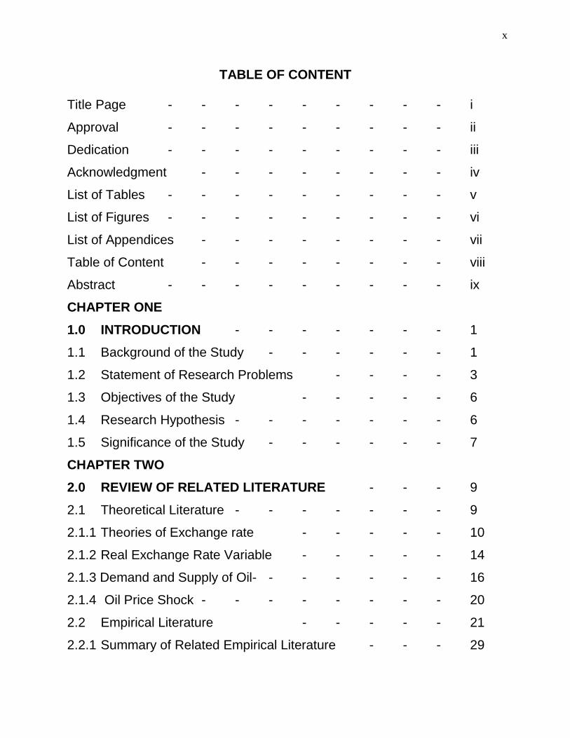
TABLE OF CONTENT
Title Page - - - - - - - - - i
Approval - - - - - - - - - ii
Dedication - - - - - - - - - iii
Acknowledgment - - - - - - - - iv
List of Tables - - - - - - - - - v
List of Figures - - - - - - - - - vi
List of Appendices - - - - - - - - vii
Table of Content - - - - - - - - viii
Abstract - - - - - - - - - ix
CHAPTER ONE
1.0 INTRODUCTION - - - - - - - 1
1.1 Background of the Study - - - - - - 1
1.2 Statement of Research Problems - - - - 3
1.3 Objectives of the Study - - - - - 6
1.4 Research Hypothesis - - - - - - - 6
1.5 Significance of the Study - - - - - - 7
CHAPTER TWO
2.0 REVIEW OF RELATED LITERATURE - - - 9
2.1 Theoretical Literature - - - - - - - 9
2.1.1 Theories of Exchange rate - - - - - 10
2.1.2 Real Exchange Rate Variable - - - - - 14
2.1.3 Demand and Supply of Oil- - - - - - - 16
2.1.4 Oil Price Shock - - - - - - - - 20
2.2 Empirical Literature - - - - - 21
2.2.1 Summary of Related Empirical Literature - - - 29
x
9
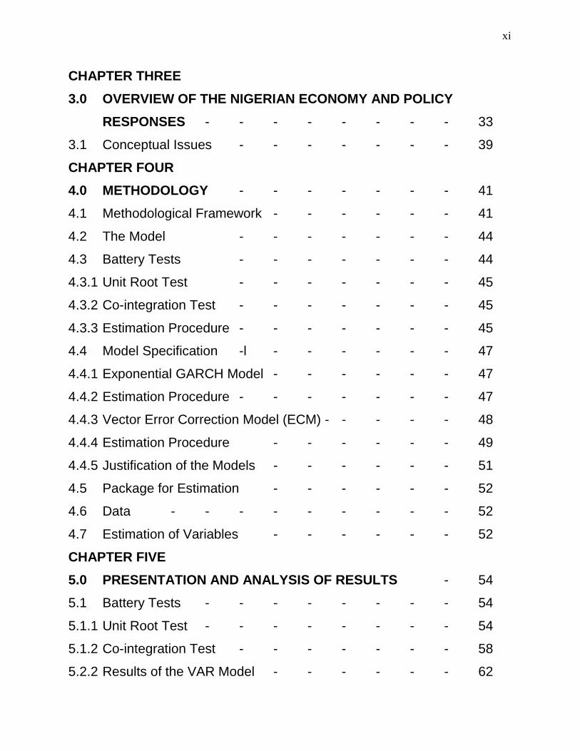
CHAPTER THREE
3.0 OVERVIEW OF THE NIGERIAN ECONOMY AND POLICY
RESPONSES - - - - - - - - 33
3.1 Conceptual Issues - - - - - - - 39
CHAPTER FOUR
4.0 METHODOLOGY - - - - - - - 41
4.1 Methodological Framework - - - - - - 41
4.2 The Model - - - - - - - 44
4.3 Battery Tests - - - - - - - 44
4.3.1 Unit Root Test - - - - - - - 45
4.3.2 Co-integration Test - - - - - - - 45
4.3.3 Estimation Procedure - - - - - - - 45
4.4 Model Specification -l - - - - - - 47
4.4.1 Exponential GARCH Model - - - - - - 47
4.4.2 Estimation Procedure - - - - - - - 47
4.4.3 Vector Error Correction Model (ECM) - - - - - 48
4.4.4 Estimation Procedure - - - - - - 49
4.4.5 Justification of the Models - - - - - - 51
4.5 Package for Estimation - - - - - - 52
4.6 Data - - - - - - - - - 52
4.7 Estimation of Variables - - - - - - 52
CHAPTER FIVE
5.0 PRESENTATION AND ANALYSIS OF RESULTS - 54
5.1 Battery Tests - - - - - - - - 54
5.1.1 Unit Root Test - - - - - - - - 54
5.1.2 Co-integration Test - - - - - - - 58
5.2.2 Results of the VAR Model - - - - - - 62
xi
10
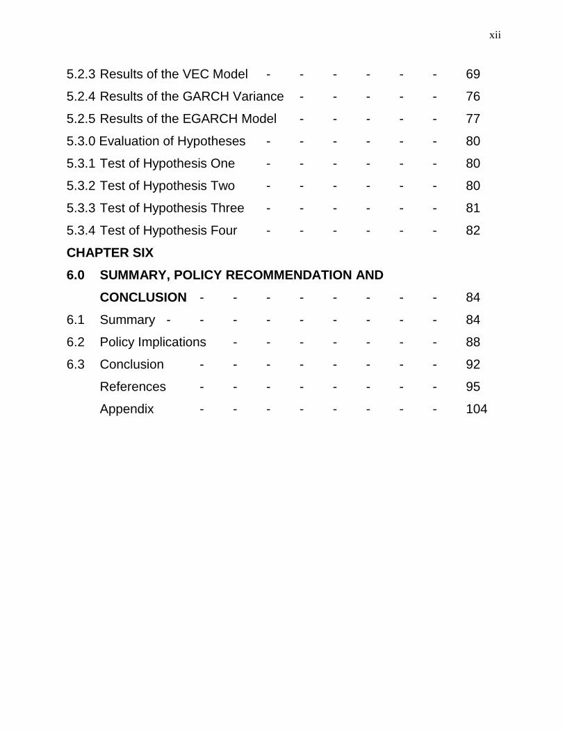
5.2.3 Results of the VEC Model - - - - - - 69
5.2.4 Results of the GARCH Variance - - - - - 76
5.2.5 Results of the EGARCH Model - - - - - 77
5.3.0 Evaluation of Hypotheses - - - - - - 80
5.3.1 Test of Hypothesis One - - - - - - 80
5.3.2 Test of Hypothesis Two - - - - - - 80
5.3.3 Test of Hypothesis Three - - - - - - 81
5.3.4 Test of Hypothesis Four - - - - - - 82
CHAPTER SIX
6.0 SUMMARY, POLICY RECOMMENDATION AND
CONCLUSION - - - - - - - - 84
6.1 Summary - - - - - - - - - 84
6.2 Policy Implications - - - - - - - 88
6.3 Conclusion - - - - - - - - 92
References - - - - - - - - 95
Appendix - - - - - - - - 104
xii
11
ABSTRACT
The rate at which different macroeconomic variables are fluctuating has constituted severe problems for policy analysis. Some macroeconomic variables‟ volatility has become a key determinant as well as a consequence of poor economic management in Nigeria. The exchange rate is arguably the most difficult macroeconomic variable to model empirically. It has been recognized that if one could find a missing real shock that were sufficiently volatile to influence exchange rate, one could potentially, take an important step towards resolving the purchasing power parity puzzle. This is why the adoption of different exchange rate regimes to minimize fluctuations in the Nigerian economy could not achieve significant results. Many researchers have used cross-country regression models to find out the causes of fluctuation in exchange rate. Many of these researches could not yield significant results because some of the techniques employed suffer from either inappropriate measurement or specification bias or both. The results may not also be robust because of the heterogeneity of macroeconomic data, especially the data from the developing countries. This study adds to the existing literature by identifying that real exchange rate fluctuation depends on the oil price fluctuation using country specific regression. It also addresses the problem of the relationship between oil price shocks and some other macroeconomic variables in Nigeria. It further addresses the problem of transmission of shocks from oil price to real exchange rate and to some macroeconomic variables. The study equally, looks at the problem of how current shocks on oil price relates with its conditional volatility in periods ahead. This work adopted the generalized Autoregressive conditional Heteroscedasticity (GARCH) variance, exponential generalized Autoregressive conditional Heteroscedasticity (EGARCH) and Vector Error correction VEC) models to capture different hypotheses specified in the work. The GARCH variance was used to explain that real exchange rate volatility might be determined by oil price volatility. The EGARCH model was used to determine whether current shock on oil price has any relationship with its conditional volatility in periods ahead. The VEC model was used to trace the transmission of shocks among the variables. The results show that oil price fluctuation positively and significantly influence real exchange rate fluctuation with z-statistic of 11.71828 and coefficient of 1.472587. It also shows that all the explanatory variables except industrial production growth rate (IPR) are statistically significant in explaining the real exchange rate. It equally, shows that there is transmission of structural shocks among the variables. The News Impact Curve (NIC) indicates that the current shock in oil price is influenced by the previous shocks and its effect on other periods‟ ahead, decays exponentially.
xiv
1
CHAPTER ONE
1.0 INTRODUCTION
1.1 Background of the Study:
There has been controversy among researchers on what policy
response that will bring about or causes fluctuations in aggregate economic
activities. Some believe that monetary policy response should be assigned
more weight, while others still argue that the fiscal policy should be the
most appropriate. Yet other researchers have identified oil price shocks as
of very great importance in influencing economic growth and aggregate
economic activities.
The current global energy crisis poses a great challenge to policy
makers across countries. The price of crude oil slumped in the world
market during the first half of 1980s. Thus, Nigeria‟s crude oil which sold at
slightly above US $41 a barrel in early 1981, fell precipitously to less than
US $9 a barrel by August 1986 (Uwubanmen 2002). The price of oil
fluctuates between $17 and $26 at different times in 2002, around $53 per
barrel by October 2004, around $89 per barrel by January 2008. In fact,
the price of oil has witnessed noticeable fluctuations since the past three
decades after the collapse of the Breton woods.
ii
2
Persistent oil shocks and exchange rate fluctuations could have
severe macroeconomic implications, thus inducing challenges for policy
making – fiscal or monetary in both the oil exporting and oil importing
countries – (Kim and Loughani 1992; Caruth, Hooker and Oswald 1996;
Hamilton 1996; Mork 1994; Taton 1988; Hooker 1996; Daniel 1997;
Cashin, Liang and Mcdermoth 2000). Some of these studies suggest rising
oil prices reduced output and increased inflation in the 1970s and early
1980s and falling oil prices boosted output and lowered inflation particularly
in the United States in the mid to late 1980s. The transmission
mechanisms through which oil prices have impact on real economic activity
include both supply and demand channels. Nigeria as an oil exporting
country that depends primarily on oil as her main source of revenue
generation (see the box below) the economic Activities will be sensitive to
oil price shocks and exchange rate fluctuations between her trading nations
as it serves as the relative price of the domestic currency.
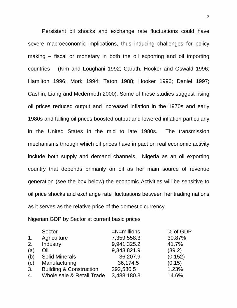
Nigerian GDP by Sector at current basic prices
Sector =N=millions % of GDP 1. Agriculture 7,359,558.3 30.87% 2. Industry 9,941,325.2 41.7% (a) Oil 9,343,821.9 (39.2) (b) Solid Minerals 36,207.9 (0.152) (c) Manufacturing 36,174.5 (0.15) 3. Building & Construction 292,580.5 1.23% 4. Whole sale & Retail Trade 3,488,180.3 14.6%
3
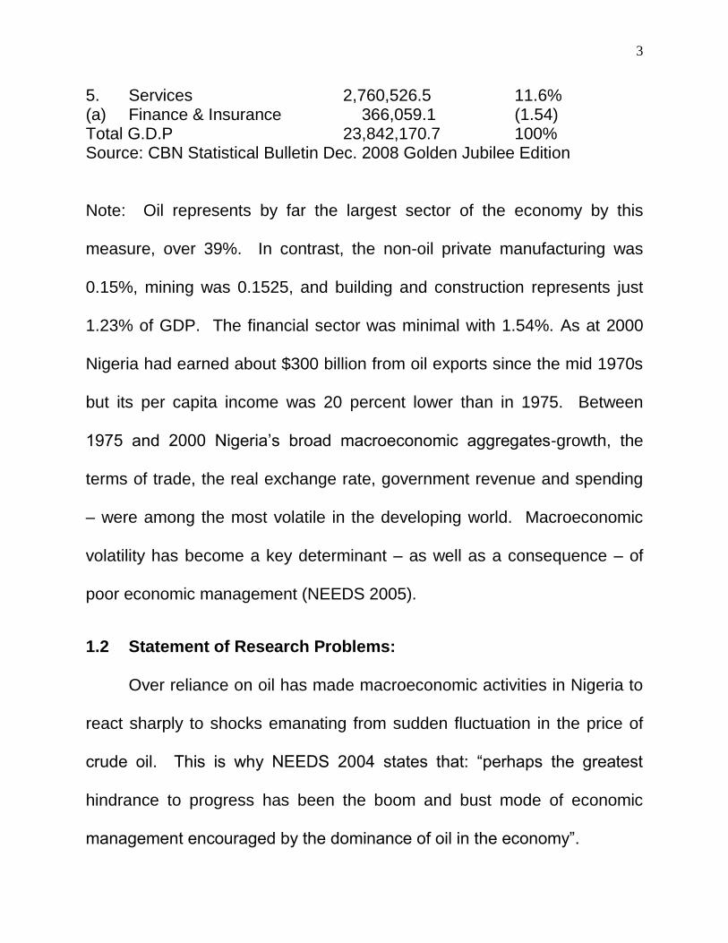
5. Services 2,760,526.5 11.6% (a) Finance & Insurance 366,059.1 (1.54) Total G.D.P 23,842,170.7 100% Source: CBN Statistical Bulletin Dec. 2008 Golden Jubilee Edition
Note: Oil represents by far the largest sector of the economy by this
measure, over 39%. In contrast, the non-oil private manufacturing was
0.15%, mining was 0.1525, and building and construction represents just
1.23% of GDP. The financial sector was minimal with 1.54%. As at 2000
Nigeria had earned about $300 billion from oil exports since the mid 1970s
but its per capita income was 20 percent lower than in 1975. Between
1975 and 2000 Nigeria‟s broad macroeconomic aggregates-growth, the
terms of trade, the real exchange rate, government revenue and spending
– were among the most volatile in the developing world. Macroeconomic
volatility has become a key determinant – as well as a consequence – of
poor economic management (NEEDS 2005).
1.2 Statement of Research Problems:
Over reliance on oil has made macroeconomic activities in Nigeria to
react sharply to shocks emanating from sudden fluctuation in the price of
crude oil. This is why NEEDS 2004 states that: “perhaps the greatest
hindrance to progress has been the boom and bust mode of economic
management encouraged by the dominance of oil in the economy”.
4
The advent of oil boom has led to a decline in the contribution of the
non-oil sectors in most of the oil exporting countries, a phenomenon
referred to as the “Dutch – Disease”. The implication of this is that while oil
price increase should be considered good news in oil exporting countries
and bad news in oil importing countries, the reverse should be expected
when oil price decreases. For instance, the downturn in the oil prices after
1980 led to disastrous economic consequences in many oil exporting
countries leading to large fiscal imbalances, poor export performance, high
level of foreign balance of account deficits, large and growing external
debts, stagflation, large and rising unemployment and alarming
deterioration of social and economic infrastructures (Jimenez and Sanchez
2003). The different transmission mechanisms of oil price shocks to the
real economy have different features in each of the countries, which thus
respond some what differently to such shocks. In light of the different levels
of oil dependence, different policies are implemented to smooth out the
consequences of such shocks in different oil exporting countries.
Exchange rate on its own part has witnessed frequent fluctuations since
after the collapse of the Breton wood.
Studies on oil price and U.S. real exchange rate have shown that the
U.S. real exchange rate is a positive function of the real oil price (Amano,
5
and Van Norden 1998; Lahtinen 2000). This positive relationship between
U.S. dollar and oil price is partly problematic because being a major
importer of crude oil, higher oil price worsens the U.S. terms of trade (Chen
and Rogoff 2001). Backus and Crucini 1998, also argue that higher oil
price should depreciate the U.S. dollar and not to appreciate it. Also relative
to the German mark, oil price changes affect negatively the United States
terms of trade than German terms of trade. In their own study, Amano and
Van Norden (1995), presents a special case for Canada, where higher oil
price led to a weaker Canadian dollar relative to U.S. dollar despite the fact
that Canada is a substantial exporter of oil and the U.S. a net importer of
crude oil. Nigeria may not be different from Canadian experience. The
increase in oil price over the years has witnessed a depreciation of naira
exchange rate to most foreign currencies such as U.S dollar, British pounds
sterling, and Euro. Based on the above discussion, this paper intends to
address the following questions.
i Can real exchange rate volatility be explained by oil price volatility in
Nigeria?
ii Is there any significant impact of oil price shocks on real exchange
rate fluctuations in Nigeria?
6
iii Do shocks transmit from oil price and real exchange rate fluctuation
to some macroeconomic variables in Nigeria?
iv What are the relationships between the current shock on oil price and
its conditional volatility in other periods ahead?
1.3 Objectives of the Study:
The broad objective of this study is to estimate the impact of oil price
shocks on real exchange rate and trace the transmission of structural
shocks from oil price to exchange rate and other factors affecting it. The
specific objectives are:
1) To determine whether real exchange rate volatility can be explained
by oil price volatility in Nigeria.
2) To determine the significant of the impact of oil price shocks on real
exchange rate fluctuations in Nigeria.
3) To trace how shocks transmit from oil price and real exchange rate
fluctuation to some macroeconomic variables in Nigeria.
4) To estimate the relationship between the current shock on oil price
and its conditional volatility in other periods ahead.
1.4 Research Hypothesis
The research hypotheses of the study are:
7
i) Real exchange rate volatility cannot be explained by oil price
volatility in Nigeria.
ii) There is no significant impact of oil price shocks on real exchange
rate fluctuations in Nigeria.
iii) There is no transmission of shocks from oil price and real
exchange rate fluctuations to some macroeconomic variables in
Nigeria.
iv) Current shock on oil price has no relationship with its conditional
volatility in other periods ahead.
1.5 Significance of the Study:
The interface between real exchange rate fluctuations and oil price
shocks has been over looked in the existing empirical literature in Nigeria in
spite of Nigeria‟s dependent on crude oil revenue.
Nigeria‟s underlying current account balance is a function of three
major determinants its oil exports, priced at a sustainable long term trend
value; the competitiveness of its non-oil exports; the pace of remittances
from Nigerians living abroad. Nigeria‟s balance of payments have been
subject to a high degree of variability caused by: variability in government
spending, which often creates surge in import payments for capital projects;
variability in the price of oil; variability in capital flight caused by periodic

8
exchange rate uncertainty. These swings are difficult to predict, but they
can have a substantial impact on monetary expansion and the exchange
rate.
Literature has shown that oil price volatility affects the real exchange
rate for Germany, Japan and the United states and not much has been said
about Nigeria. Many studies used cross-country regression to study the link
between exchange rate fluctuations and macroeconomic activities of
various countries. The result of cross-country regression is prone to biased
ness as a result of the heterogeneous nature of data obtained in less
developed countries. Most of the studies reviewed were on oil importing
countries.
These create a need for this study that uses country-specific
regression to determine the impact of oil price shocks on real exchange
rate fluctuations in Nigeria. The ability of the models in this work to
determine the conditional volatility of current real exchange rate and to
trace the relationship between current shocks on oil price and its
conditional volatility in periods ahead make this work very important and
will help to ginger a policy debate in the area. This is equally, very vital for
policy forecasting and adjustment especially in this era where every country
is aiming at targeting rules.
9
CHAPTER TWO
2.0 REVIEW OF RELATED LITERATURE
2.1 Theoretical Literature:
Hooper and Mann (1989) and Blundell – Wignall and Browne (1991)
spearheaded the works on the fundamental determination of the real
exchange rate. The identified fundamentals are real interest rate
(differentials) and current account imbalances. The model asserts that
shocks that drive the exchange rate away from the fundamentals will
ultimately release it back to levels projected by those variables. There are
number of factors that might be associated with the long-run real exchange
rate in transition economies (Motiel 1999). First, domestic supply side
factors should be considered, especially variables related to the Balassa –
Samuelson effect (Note: The Balassa – Samuelson theorem assumes that
purchasing power parity (PPP) holds for the market of traded goods, but
that ratio of prices of traded and non-traded goods may evolve differently in
one country than in another, as productivity in poorer countries grows faster
in the traded-goods sector than in the non-traded goods sector. The
potential for productivity growth in the traded goods sector of poorer
countries is higher than in richer countries. It is further presumed that
productivity in the non-traded sector rises more slowly, while wages remain
10
the same in both sectors. In such cases, the real exchange rate
appreciates in the country with higher growth).
Second, demand – side factors may be important, such as fiscal
policy measures that induce changes in the composition of government
spending between traded goods and non-traded goods. (Note: if the
income elasticity of non-traded goods is larger than unity then their relative
price will move along with living standards which will cause appreciation of
the real exchange rate. Further, if government expenditure is biased
toward traded goods and the share of government expenditure in GDP
increases over time, the real exchange rate will depreciate).
Other proposed factors include changes in the international economic
environment (e.g. terms of trade), net foreign assets, and trade openness.
(Note: for example, if trade regime is more open, it is likely to expect the
real exchange rate depreciation. Trade restrictions may increase domestic
prices of traded goods, which further leads to rise in composite price index
and the real exchange rate appreciation) (Zorica Mladenovic 2004)
2.1.1 Theories of Exchange Rate:
Milton Friedman (1953), an early advocate of flexible exchange rates,
argue that one advantage of floating rates is that they could allow rapid
change in relative prices between countries: “A rise in the exchange rate ---
11
makes foreign goods cheaper in terms of domestic currency, even though
their prices are unchanged in terms of their own currency, and domestic
goods more expensive in terms of foreign currency, even though their
prices are unchanged in terms of domestic currency; this tends to increase
imports and reduce exports” (Friedman, 1953: 162). This passage makes
two assumptions; that goods prices are unchanged in the currency of the
producer of the good, and that there is significant pass-through of the
exchange rate change to the buyer of the good. On the nominal price
stickiness, Friedman argues that the choice of exchange rate regime would
matter little if nominal goods prices adjusted quickly to shocks. He argues
that, “if internal prices were as flexible as exchange rates, it would make
little economic difference whether adjustments were brought about by
changes in exchange rates or by equivalent changes in internal prices. But
this condition is clearly not fulfilled. At least in the modern world, internal
prices are highly inflexible”.
In assessing this relative-price effect and its significant for the choice
of exchange-rate regime, Friedman is certainly correct to emphasize the
importance of normal goods price stickiness. As Buiter (1999), has
forcefully emphasized, the decision to join a monetary union, or the choice
of an exchange rate regime is a monetary issue. Relative-price behaviour
12
is usually independent of monetary regime in a world of perfect goods price
flexibility. The pioneering work of Obstfeld and Rogoff (1995, 1998, 2000a)
has assumed that nominal prices are fixed in the producer‟s currencies, so
that price for consumers change one – for – one in the short-run with
changes in the nominal exchange rate. This is exactly the assumption of
Friedman.
Another theory of exchange rate is the Purchasing Power Parity
(PPP). This concept PPP is often used as an analytical tool to explain and
predict movements in exchange rates. Two types of PPP can be
distinguished: absolute PPP and relative PPP. (Note: The purchasing
power parity between any two countries is the number of units of the one
country‟s currency (e.g. naira) which endows the holder with the same
purchasing power (i.e. command over goods and services) as one unit of
the other country‟s currency (e.g. U.S. dollar). PPP can be between two
countries, in which case it is a bilateral comparison, or to parity between
the country and a group of trading partners, in which case it is a multilateral
comparison). According to the absolute PPP theory the “equilibrium”
exchange rate between two currencies is set by the ratio between the price
levels in the two countries. Thus, if goods cost more in the United States
than in Nigeria (with prices in both countries expressed in dollars, using the
13
prevailing exchange rates), the naira is under valued relative to the dollar.
Similarly, if dollar prices of goods are lower in the United States, than in
Nigeria the naira is overvalued against the dollar. Price indices are
insufficient to calculate an absolute PPP, so a cost of a basket of goods
and services is employed. For example, let us assume the cost of a basket
in January 2006 was $60 in United States and N6480 in Nigeria. These
figures imply a purchasing power parity exchange rate of $1 = 60
6480N =
N108 whereas the exchange rate prevailing at the time was about $1 =
N168.
The relative PPP theory states that changes in rates reflect
differences in relative inflation rates. Relative PPP is thus concerned with
the ratio of the equilibrium exchange rate in a current period relative to the
equilibrium exchange rate in a base period. According to this theory, PPP
is determined by the ratio of the domestic country‟s price index in the
current period to the foreign country‟s price index in the same period,
where both indices have a common base period. Thus, if dollar prices
have risen at a slower rate in the United States than naira prices have risen
in Nigeria, the dollar should appreciate against the naira compared to the
exchange rate in the common base period. Another theory is the theory of
incomplete pass-through. This theory has been addressed in various ways
14
in the literature. The most common analytical tool to examine incomplete
pass-through has probably been pricing-to-market approach that
presupposes short-term rigidities and the market power of importing
companies. These market imperfections allow foreign suppliers to set the
markup of prices over the marginal cost. According to the pricing-to-market
approach, international markets for manufacturing goods are sufficiently
segmented that producers or retailers can, at least over some horizon,
tailor the prices they charge to the specific local demand conditions
prevailing in different national markets. Thus, firms set different prices for
their goods across segmented national markets to compete with firms in
those markets. According to Dornbush (1987), the degree of pass-through
depends on (i) substitution between domestic and foreign goods (ii) market
integration (iii) market organization. Evidence seems to suggest that the
dominant component of real exchange rate behaviour is a nominal
exchange rate even in a long-run through the incomplete pass-through
(Asea and Mendoza 1994; De-Gregorio and Wolf 1994).
2.1.2 Real Exchange Rate Variable
The real exchange rate is a measure of one country‟s overall price
level relative to another country. The real exchange rate, defined with
15
respect to a general or overall price level, such as the consumer price
index (CPI) (Lahtinen 2001), is given by
qt = Pt – Pt* - St - - - - - - - - - - - - - (1)
where qt denotes the logarithm of real exchange rate, Pt denotes the log of
the domestic price level,, Pt* the log of the foreign price level and St the log
of the nominal exchange rate defined as the home currency price of a unit
of foreign currency. In this context therefore, a rise in qt denotes an
appreciation of the real exchange rate. To measure the price level,
decompose it into the traded and non-traded components and use a
geometric average of these prices in both country.
Pt = (1- ) PtT + Pt
N, < 1 -------------- (2)
where Pt denotes the logarithm of the price index, PtT is the log of the
traded goods price index, PtN is the log of the non-traded goods price index
and is the share that non-traded goods take in the price index. Letting an
asterisk represent the foreign country, one can also write;
Pt* = (1-β) Pt
T* + βPtN*, β < 1 ----------- (3)
where β is non-traded good‟s share in the foreign price index.
Thus, following Engel (1999), the real exchange rate can be written
as
qt = xt + Yt ------------------------------- (4)
where
Xt = PtT - Pt
T* - St ---------------------- (5) and
16
Yy = (PtN* - Pt
T*) -------------------- (6)
Yt defines a traditional Harrods – Balassa Samuelson condition, which
relates labour productivity to non-tradable goods prices.
Xt is the deviations from the law of one price for tradable goods.
The real exchange rate models, such as traditional Harrods – Balassa –
Samuelson Model, adequately explain only a few bilateral real exchange
rates during a few sub periods. If there were no relative structural shocks
between two currency areas, a real exchange rate should be a stationary
variable and it should follow the purchasing power parity hypothesis.
Demand and Supply of Oil
On the other hand, oil is arguably the quaint essential commodity in
the modern industrial economy. Although the industrial revolution was
initially powered by coal, since its discovery in Pennsylvania in 1869, oil
has gained increasing prominence in terms of its share of the world‟s
primary energy supply, accounting for 37 percent (the largest share) in
2001 (IEA, 2005). As an energy source, oil is used for electricity
generation, and to a lesser extent for heating and cooking. However, its
most important role is as a liquid fuel for transportation. Globally, ship,
train, airplane and road transport depend mainly on oil. Consequently, the
tourism sector in most countries is also highly reliant on oil. Industrial
17
agriculture (or agri-business) depends heavily on oil for the production of
fertilizers, herbicides and pesticides. The manufacturing sector uses oil
both for energy and as a feedstock for a myriad of products from plastics to
paints to pharmaceuticals.
Historically there have been three eras in the determination of
international crude oil prices (Nkomo, 2006). Price of oil was determined
chiefly by multinational oil companies, until in 1970, when the Organization
of Petroleum Exporting Countries (OPEC) asserted its capacity to influence
the price via its output decisions. Since the late 1980s, however, “world oil
prices have been set by a market-related pricing system which links oil
prices to the „market price‟ of a particular reference crude” (Farrell, Kahn
and Visser 2001: 69). Two important reference prices, Brent and West
Texas intermediate (WTI), are determined on the London and New York
futures exchanges respectively.
The fundamental determinant of oil prices is the demand/supply
balance in the international market; each side of this market is in turn
influenced by several factors. Over the long-term, the demand for oil is
determined primarily by rates of economic growth in the major regions of
the world, as well as by energy-related technological developments such as
efficiency gains or new found uses for oil. Such structural determinants
18
tend not to change rapidly and are therefore unlikely to provide the impetus
for an oil price shock on their own. However, China‟s extraordinary growth
has had an increasingly significant effect on the world demand for oil, most
notably in 2004. The supply side of the crude oil market is comprised of
output from OPEC and non-OPEC producing countries, whose production
decisions hinge on geological, economic and political factors (Farrell et al
2001: 72 – 78). In the long-term, oil supply depends on the rates of
extraction, depletion, and new discoveries, as well as developments in
extractive technologies that allow enhanced recovery of oil. In the short-
term, changes in OPEC production quotas and temporary supply
disruptions due to technical or political factors or natural disasters can have
important consequences for supply and hence oil prices.
In addition to these fundamentals, expectations and speculation
about future demand and (especially) supply conditions – which in turn are
stimulated by economic and political conditions – play a large part in the
determination of crude oil prices on the futures and spot markets,
particularly when inventories are low (Nkomo, 2006: 13; Farrell et al, 2001:
82). These considerations also amplify oil price volatility.
The balance between supply and demand in the oil market has been
gradually tightening over the past few years. This is partly attributable to
19
steeply rising demand on the back of robust economic growth, especially in
major emerging economies, such as China, but also in the U.S. On the
other hand, supply has expanded less rapidly than demand. Moreover,
there have been temporary or recurrent disruptions to the flow of oil in
some areas as a result of various factors, such as: the ongoing conflict in
Iraq; sporadic conflict and sabotage in Nigeria; the devastation wrought by
Hurricanes, Katrina and Rita in the Gulf of Mexico; and a leaking pipeline
leading to a temporary closure of the Prudhoe Bay field in Alaska in August
2006. Speculation in the oil market has amplified the price effects of these
relatively minor supply disruptions. In addition, fears amongst oil traders
were exacerbated by the conflict between Israel and Hezbellah in
July/August 2006 (Wakeford 2006). As a consequence, the price of crude
oil rose from around US $25 per barrel in 2003 to a high point of US $78
per barrel in July 2006, and about US $98 per barrel in January 2008. this
represents roughly four-times of oil prices over four years which may be
defined as a „trend‟ oil price shock.
It is also important to notice that the time path of oil price is not
determined in a competitive market. Although, we do not argue that oil
prices are immune to the laws of supply and demand, it seems to be a
quite reasonable argument that oil prices are strongly dependent on the
20
stability of cartels. The most important cartel for an oil price is obviously
the OPEC cartel. This cartel does not have all the elements of a successful
cartel because it is simply too fragmented culturally and politically
(Wakeford 2006). However, the history of the rise and fall of oil prices is
also very suggestive of some sort of multiple equilibrium stories. Some
analyses indicate that the historical behaviour of oil prices do not allow one
to predict how future oil prices will fluctuate. The severity of movements of
price do not provide any information about their future likely duration and
the time spent in a current boom or slump provide no information about the
likely future duration of that boom or slump. Indeed the collapse of oil
prices in 1986 also came with dramatic suddenness, again suggestive of a
collapse of an equilibrium and establishment of another. This possible
multiple equilibrium nature of the oil price makes it a very unstable variable
with possible jumps in the price process.
2.1.3 Oil Price Shocks
Oil shocks are usually defined in terms of price fluctuations, but these
may in turn emanate from changes in either the supply of or the demand for
oil. In practice it is unlikely for demand to grow rapidly enough to cause a
price shock unless it is motivated by fears of supply shortages. Oil price
shocks may of course be negative (a fall) or positive (a rise). There are at
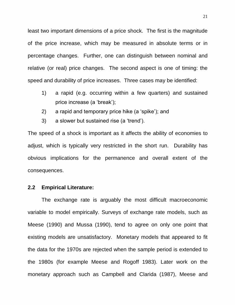
21
least two important dimensions of a price shock. The first is the magnitude
of the price increase, which may be measured in absolute terms or in
percentage changes. Further, one can distinguish between nominal and
relative (or real) price changes. The second aspect is one of timing: the
speed and durability of price increases. Three cases may be identified:
1) a rapid (e.g. occurring within a few quarters) and sustained
price increase (a „break‟);
2) a rapid and temporary price hike (a „spike‟); and
3) a slower but sustained rise (a „trend‟).
The speed of a shock is important as it affects the ability of economies to
adjust, which is typically very restricted in the short run. Durability has
obvious implications for the permanence and overall extent of the
consequences.
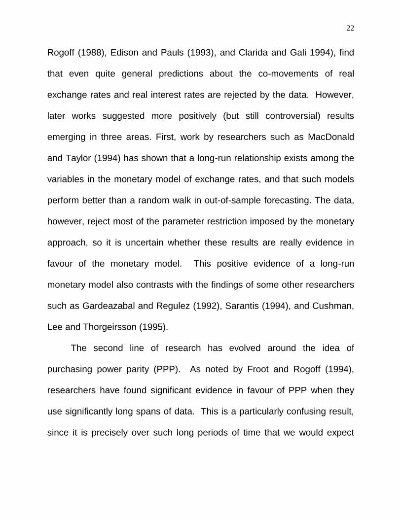
2.2 Empirical Literature:
The exchange rate is arguably the most difficult macroeconomic
variable to model empirically. Surveys of exchange rate models, such as
Meese (1990) and Mussa (1990), tend to agree on only one point that
existing models are unsatisfactory. Monetary models that appeared to fit
the data for the 1970s are rejected when the sample period is extended to
the 1980s (for example Meese and Rogoff 1983). Later work on the
monetary approach such as Campbell and Clarida (1987), Meese and
22
Rogoff (1988), Edison and Pauls (1993), and Clarida and Gali 1994), find
that even quite general predictions about the co-movements of real
exchange rates and real interest rates are rejected by the data. However,
later works suggested more positively (but still controversial) results
emerging in three areas. First, work by researchers such as MacDonald
and Taylor (1994) has shown that a long-run relationship exists among the
variables in the monetary model of exchange rates, and that such models
perform better than a random walk in out-of-sample forecasting. The data,
however, reject most of the parameter restriction imposed by the monetary
approach, so it is uncertain whether these results are really evidence in
favour of the monetary model. This positive evidence of a long-run
monetary model also contrasts with the findings of some other researchers
such as Gardeazabal and Regulez (1992), Sarantis (1994), and Cushman,
Lee and Thorgeirsson (1995).
The second line of research has evolved around the idea of
purchasing power parity (PPP). As noted by Froot and Rogoff (1994),
researchers have found significant evidence in favour of PPP when they
use significantly long spans of data. This is a particularly confusing result,
since it is precisely over such long periods of time that we would expect
23
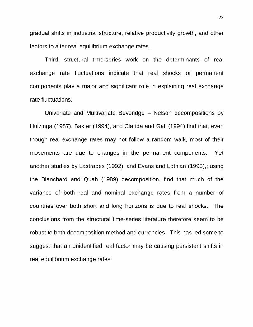
gradual shifts in industrial structure, relative productivity growth, and other
factors to alter real equilibrium exchange rates.
Third, structural time-series work on the determinants of real
exchange rate fluctuations indicate that real shocks or permanent
components play a major and significant role in explaining real exchange
rate fluctuations.
Univariate and Multivariate Beveridge – Nelson decompositions by
Huizinga (1987), Baxter (1994), and Clarida and Gali (1994) find that, even
though real exchange rates may not follow a random walk, most of their
movements are due to changes in the permanent components. Yet
another studies by Lastrapes (1992), and Evans and Lothian (1993),; using
the Blanchard and Quah (1989) decomposition, find that much of the
variance of both real and nominal exchange rates from a number of
countries over both short and long horizons is due to real shocks. The
conclusions from the structural time-series literature therefore seem to be
robust to both decomposition method and currencies. This has led some to
suggest that an unidentified real factor may be causing persistent shifts in
real equilibrium exchange rates.
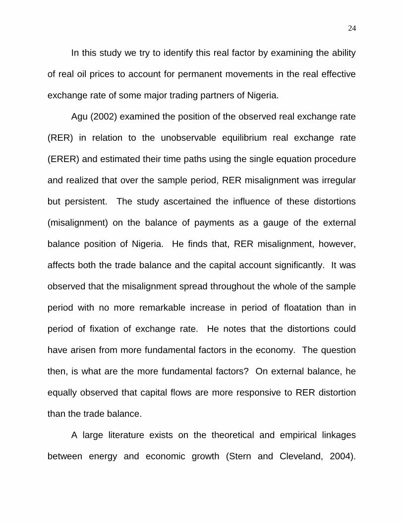
24
In this study we try to identify this real factor by examining the ability
of real oil prices to account for permanent movements in the real effective
exchange rate of some major trading partners of Nigeria.
Agu (2002) examined the position of the observed real exchange rate
(RER) in relation to the unobservable equilibrium real exchange rate
(ERER) and estimated their time paths using the single equation procedure
and realized that over the sample period, RER misalignment was irregular
but persistent. The study ascertained the influence of these distortions
(misalignment) on the balance of payments as a gauge of the external
balance position of Nigeria. He finds that, RER misalignment, however,
affects both the trade balance and the capital account significantly. It was
observed that the misalignment spread throughout the whole of the sample
period with no more remarkable increase in period of floatation than in
period of fixation of exchange rate. He notes that the distortions could
have arisen from more fundamental factors in the economy. The question
then, is what are the more fundamental factors? On external balance, he
equally observed that capital flows are more responsive to RER distortion
than the trade balance.
A large literature exists on the theoretical and empirical linkages
between energy and economic growth (Stern and Cleveland, 2004).
25
Energy (especially oil) is a critical input in many productive processes and
therefore a causal factor for economic growth; in addition, economic growth
stimulates the consumption of oil by households. It is small wonder
therefore, that demand, supply and price of crude oil attracts so much
attention. There have been several studies on the link between oil prices
and U.S. macroeconomic aggregates (for example, Hamitton 1983,
Loungani 1986, Dotsey and Reid 1992), but exchange rates were not
included and evidence for other nations is lacking.
There has also been some analysis with calibrated macro-models (McGuirk
1983 and Yoshikawa 1990) which suggest that oil price fluctuations play an
important role in exchange rate movements, but these studies lack
econometric rigor and consider a data sample limited either in length or
number of currencies. Some studies such as Throop (1993), Zhou (1995),
and Dibooglu (1995) find evidence of a long-run relationship between
exchange rates and a number of macroeconomic factors including oil
prices. However, the tests used in these studies tend to produce false
evidence of co-integration when several variables are included in the
system (Gonzalo and Pitarakis 1994, and Godbout and Van Norden 1995).
They do not examine the causal relationship between these variables, so it
is not clear whether these are models of exchange rate determination, or
26
whether they simply capture the influence of exchange rates on a variety of
other macroeconomic variables. In another study by JEL (1996), testing for
co-integration between exchange rates and oil prices using the two-step
single equation approach developed by Engle and Granger (1987) show
strong evidence of co-integration between the price of oil measures and the
real effective exchange rates for Germany, and Japan but not for the
United States. On their further test using the augmented Dickey and Fuller
(1979) and Phillips and Ouliaris (1990) tests reject the null hypothesis of no
co-integration at the one percent level for the mark, and the five and one
percent level for the Yen. They further compare these conclusions using
an efficient (and therefore more powerful) co-integration test developed by
Johansen and Juselius (1990), the tests find evidence consistent with co-
integration for all three currencies suggesting that the price of oil captures
the permanent innovations in the real exchange rate for Germany, Japan
and the United states.
It has long been recognized that if one could find a missing real shock
that were sufficiently volatile, one could potentially take an important steps
towards resolving the PPP puzzle. Real oil price has the volatility and there
is some evidence that it is an important factor modeling the U.S. real
exchange movements. In articles such as Amano and Van Norden (1998),
27
and Lahtinen (2000), the U.S. real exchange rate is shown to be a positive
function of the real oil price, i.e. higher oil price will appreciate the U.S. real
exchange rate. Lahtinen (2000) also finds support for Harrod-Balassa –
Samuelson hypothesis if the oil price is included in the estimations. These
finding have shown to be stable, which seems to suggest that the failure of
exchange rate models to provide stable results is due to the missing
variable problem. The net effect of oil price shock on nominal exchange
rate depends on capital account changes i.e. whether, for example,
investment in dollar currency is more or less than America‟s share of the
industrial world‟s current account deficit. The unstable and unpredictable
nature of the oil price process makes it also a textbook example of the non-
discrete jump process. Krugman (2000), offers a multiply equilibrium
explanation for the oil price. On the other hand, a vast literature studying
exchange rate prediction has concluded that the best single predictor of the
exchange rate next period-tomorrow, next week, next month, maybe even
next year – is the exchange rate this period. One generally cannot do
better than a “no change” forecast for exchange rates (Meese and Rogoff
1983; Cheung et al 2002). The problem here is still the inability to find the
missing link.
28
In their own study, Olomola and Adejume (2006), using vector
autoregressive (VAR) model of the Nigerian economy, find that oil price
shocks do not have substantial effects on output and inflation rate in
Nigeria over the period covered by their study. Inflation rate depends on
shocks to output and the real exchange rates. However, their findings
demonstrated that fluctuations in oil prices do substantially affect the real
exchange rates in Nigeria. It was found out that it is not the oil price itself
but rather its manifestation in real exchange rates and money supply that
affects the fluctuations of aggregate economic activity proxy, the GDP.
They conclude that oil price shock is an important determinant of real
exchange rates and in the long-run money supply, while money supply
rather than oil price shocks that affects output growth in Nigeria. The
research ignored some important variables such as trade openness, terms
of trade, trade balance capital account that may contribute to explain the
transmission of the oil price shock to real exchange rate. One can say that
the study did not adequately capture the external sector of the economy,
hence the need to close the gap. Again, most of the available literatures
were on the demand side effect, that is, oil importing countries. There is
every need for us to look at the supply side effect, that is, the oil exporting
29
countries especially Nigeria as her major source of revenue comes from
crude oil exportation.
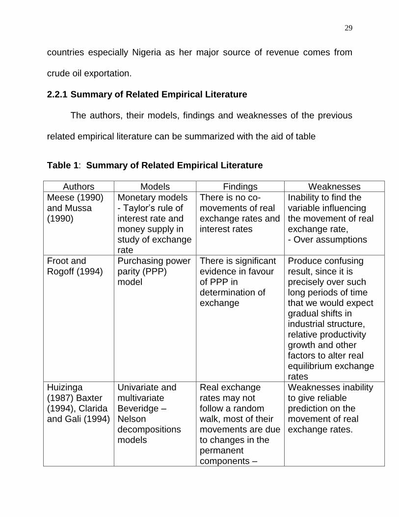
2.2.1 Summary of Related Empirical Literature
The authors, their models, findings and weaknesses of the previous
related empirical literature can be summarized with the aid of table
Table 1: Summary of Related Empirical Literature
Authors Models Findings Weaknesses
Meese (1990) and Mussa (1990)
Monetary models - Taylor‟s rule of interest rate and money supply in study of exchange rate
There is no co-movements of real exchange rates and interest rates
Inability to find the variable influencing the movement of real exchange rate, - Over assumptions
Froot and Rogoff (1994)
Purchasing power parity (PPP) model
There is significant evidence in favour of PPP in determination of exchange
Produce confusing result, since it is precisely over such long periods of time that we would expect gradual shifts in industrial structure, relative productivity growth and other factors to alter real equilibrium exchange rates
Huizinga (1987) Baxter (1994), Clarida and Gali (1994)
Univariate and multivariate Beveridge – Nelson decompositions models
Real exchange rates may not follow a random walk, most of their movements are due to changes in the permanent components –
Weaknesses inability to give reliable prediction on the movement of real exchange rates.
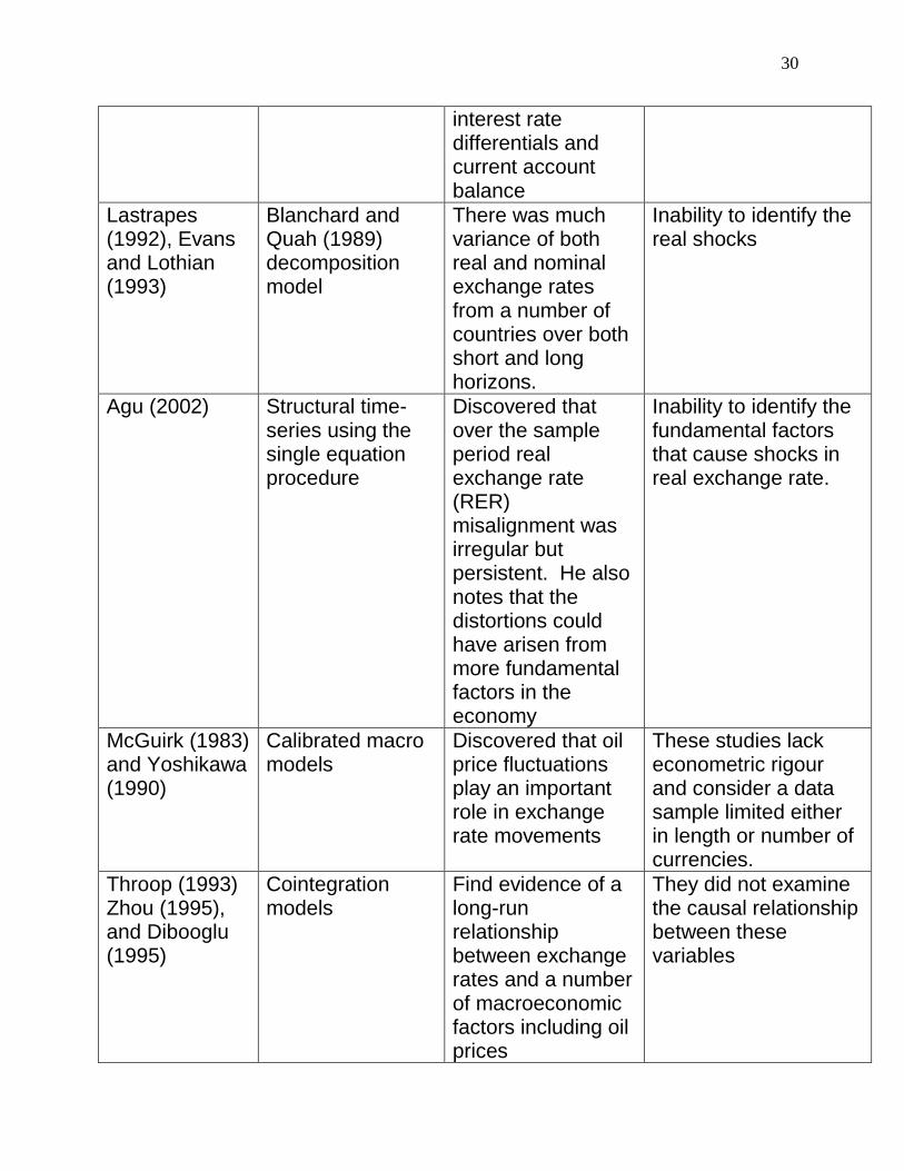
30
interest rate differentials and current account balance
Lastrapes (1992), Evans and Lothian (1993)
Blanchard and Quah (1989) decomposition model
There was much variance of both real and nominal exchange rates from a number of countries over both short and long horizons.
Inability to identify the real shocks
Agu (2002) Structural time-series using the single equation procedure
Discovered that over the sample period real exchange rate (RER) misalignment was irregular but persistent. He also notes that the distortions could have arisen from more fundamental factors in the economy
Inability to identify the fundamental factors that cause shocks in real exchange rate.
McGuirk (1983) and Yoshikawa (1990)
Calibrated macro models
Discovered that oil price fluctuations play an important role in exchange rate movements
These studies lack econometric rigour and consider a data sample limited either in length or number of currencies.
Throop (1993) Zhou (1995), and Dibooglu (1995)
Cointegration models
Find evidence of a long-run relationship between exchange rates and a number of macroeconomic factors including oil prices
They did not examine the causal relationship between these variables
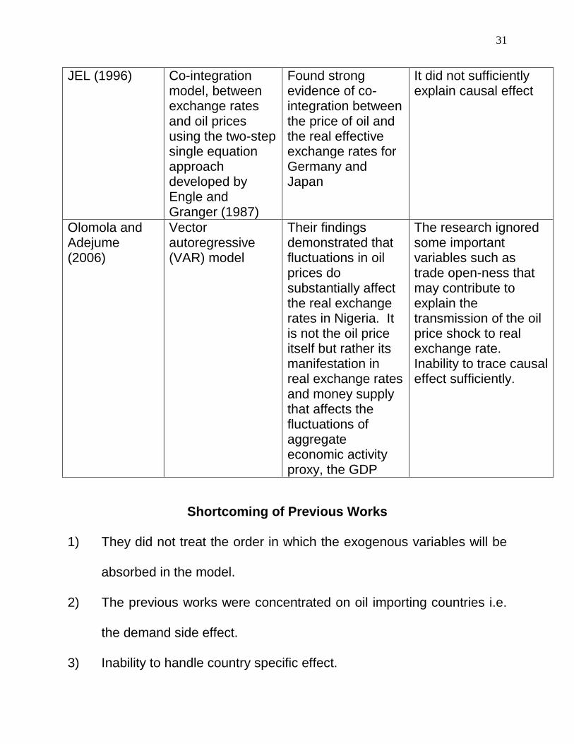
31
JEL (1996) Co-integration model, between exchange rates and oil prices using the two-step single equation approach developed by Engle and Granger (1987)
Found strong evidence of co-integration between the price of oil and the real effective exchange rates for Germany and Japan
It did not sufficiently explain causal effect
Olomola and Adejume (2006)
Vector autoregressive (VAR) model
Their findings demonstrated that fluctuations in oil prices do substantially affect the real exchange rates in Nigeria. It is not the oil price itself but rather its manifestation in real exchange rates and money supply that affects the fluctuations of aggregate economic activity proxy, the GDP
The research ignored some important variables such as trade open-ness that may contribute to explain the transmission of the oil price shock to real exchange rate. Inability to trace causal effect sufficiently.
Shortcoming of Previous Works
1) They did not treat the order in which the exogenous variables will be
absorbed in the model.
2) The previous works were concentrated on oil importing countries i.e.
the demand side effect.
3) Inability to handle country specific effect.
32
4) The previous works could not trace the sources of real exchange rate
fluctuations through monetary models, PPP models and country
specific regression
5) Available work received could not trace the transmission of structural
shocks in real exchange rate and factors affecting it.
6) The relationship between current shock on oil price and its conditional
volatility in other periods ahead was not emphasized.
There is no much work on Exchange rate fluctuations and oil price and the
very few existing work did not use oil price shocks as an explanatory
variable in their model.
33
CHAPTER THREE
3.0 OVERVIEW OF THE NIGERIAN ECONOMY AND POLICY
RESPONSES
The major sources of government finances are oil and non-oil
revenues. The oil revenue includes proceeds from sales of crude oil,
petroleum profit tax (PPT), rents and royalties while the components of
non-oil revenue are companies income tax, customs and excise duties,
value-Added Tax (VAT) and personal income tax. Since the 1970s, oil
revenue has been the dominant source of government revenue,
contributing over 70 percent to federally collected revenue.
For the need to diversify the economy, foster rapid and sustainable
real growth, since after independence in 1960, the country has embarked
on many development plans. The first was the 1962-1968 plan that was
broadly expected to facilitate the achievement and maintenance of a high
rate of increase in the standard of living as well as provide necessary
conditions for wealth creation. The plan was met with many obstacles. Fifty
percent of the planned revenue was expected to come from external
sources in the form of aid and loans, much of which was never realized.
For this, annual average planned investment for the public sector was
never achieved. Again the political crisis in 1966 that ended up in civil war

34
marred the plan. In spite of all these obstacles, the plan recorded
successes in completion of the Port-Harcourt oil refinery; the Nigerian
security printing and minting plant; the Nigerian paper mill, Jebba; the
sugar company, Bacita; the Kainji Dam; the Niger Bridge Onitsha.
The second post-independence plan, the 1970-1974 was designed,
among other things, to provide a blue print for the task of reconstruction,
rehabilitation and reconciliation. The plan envisaged an average rate of
growth in real GDP of 6.6 percent. The target was exceeded as an average
growth rate of 8.2 percent was achieved. This significant achievement
came from unprecedented inflow of crude oil money. The original planned
expenditure was revised upwards by the availability of funds.
The third national development plan 1975-1980 was launched to use
the huge foreign reserves accumulated from the oil sales to provide
employment opportunities, to enhance the diversification of the economy,
to encourage balanced development and indigenization of the economy.
The implementation of the plan suffered a major financial set back owing to
the glut in the world crude oil market. To meet with the financial demand of
the plan, the government went into massive borrowing from the Eurodollar
market and from multi-national institutions. The economy was plunged into
35
debt. The projected 9.5 percent annual average growth rate of the GDP
was never achieved instead it declined from 8.2 percent to 5.5 percent.
The economy already in Debt trap, the fourth national development
plan 1981-1985 was launched amidst serious financial constraints. The
plan was designed to reduce the dependence of the economy on a narrow
range of activities, and to develop the technological base and thereby
increase productivity. The plan targets were not realized owing largely to
financial constraints. The world crude oil market had virtually collapsed, so
oil money was not coming, as it should be. The GDP declined in real terms
by 2.9 percent during the plan period as against the 4.0 percent increase
projected (CBN2000). The government went into a second round of
borrowing under the cover that Nigeria was “under-borrowed” to increase
the government foreign debt outstanding. Thus, the problem of the poor
performance of the plan was compounded with high debt overhang.
In 1986-1988, the government introduced the structural Adjustment
Programme. Hither to, the government had introduced austerity measures
by the end of 1985 to cut down consumer goods expenses in order to
encourage savings and investments. The structural Adjustment Programme
(SAP) was put in place with a view to removing, cumbersome
administrative controls and adopting more market-friendly measures and
36
incentives that would encourage private enterprise and more efficient
allocation and use of resources. The objectives of SAP among others
include
(i) Restructuring and diversifying the productive base of the
economy in order to reduce its dependence on the oil sector
and on imports,
(ii) Achievement of fiscal and balance of payments viability in the
short to medium term.
One of the major policy instruments employed to address these
objectives was exchange rate adjustment that resulted in a drastic
devaluation of the Naira vis-à-vis major trading currencies. This was aimed
at removing what the government observed as persistent over-valuation
hitherto induced by exchange controls.
A three-year rolling plan was adopted in the management of the
economy and it took effect from the end of 1988. One of the reasons for the
adoption of a rolling plan was that it was becoming increasingly difficult to
project resources over a long period, especially for a mono-cultural
economy that relied on crude oil, whose market had been very volatile and
over which the authorities had no control. The three-year rolling plan (1990-
37
92) was first formally launched in 1990 with the primary objective of
consolidating the achievement of the SAP.
Since inception, the rolling plans have been guided by the policy of
economic deregulation and the need for rapid economic recovery. The high
dependence of the economy on the sale of crude oil in the world market
makes it imperative to examine the indicators of a country‟s external sector
performance. The external sector reflects the economic transactions
between the residents of an economy and the rest of the world. The sector
can be in equilibrium or disequilibrium (surplus or deficit). An ideal external
sector is one that is stable and in equilibrium overtime. Equilibrium is
achieved when external receipts and payments are equal, the exchange
rate is not misaligned and stable and external reserves are adequate. A
state of equilibrium may not necessarily elicit policy actions, a state of
disequilibrium calls for urgent action to reverse the trend. The ability of
policy makers to introduce such timely and appropriate measures often
determines the speed at which equilibrium is restored. The management of
the external sector aggregates-exchange rate, external reserve and
external debt-could help in reversing trends in the balance of payments.
In a policy of deregulation the exchange rate is determined by market
forces but that is not totally the case with the country, there is duality of
38
exchange rate in the foreign exchange market. The foreign exchange
market was made up of two principal segments, the official and the parallel
market, between 1960 and 1985. During this period, a fixed exchange rate
system was in place. At the end of 1998, the market was made up of the
official, Bureau de change, inter-bank, Autonomous Foreign Exchange
Market (AFEM) and the parallel segments. In the official foreign exchange
market, the exchange rate is fixed while a market determined exchange
rate is applied in the other segments. Over the years the exchange rate has
been fluctuating, for examples, an average exchange rate of N0.8938 to
US$1 in 1985, the naira exchange rate went up to N2.0206 to US$1 in
1986. In 1987 it went up to N4.0179 to US$1. In 1990 it was N7.5916 to
US$1. In 1993 it was N22.1105 to US$1. The naira exchange rate to a US
dollar, keep increasing in nominal value and the real value keep
decreasing.
The exchange rate fluctuation is demand propelled and the supply of
foreign exchange is mainly determined by the sale of crude oil whose price
is determined by the world oil market. The exchange rate volatility cannot
be stable through exchange rate management alone but could be achieved
through increased non-oil export receipts, especially of the basket of
39
currencies-US dollar, British pound sterling, German Deutschemark, Swiss
Francs, French Francs, Japanese yen and Dutch guilder.
The Nigerian oil sector has a lot of contradictions that play, a major
role in naira exchange rate. The contradiction is more glaring with rise in
crude oil price at the global market; the rise will mean more external
earnings for Nigeria but will increase the expense burden on imported
refined petroleum products. This has been so because our local refineries
are not in operation and we rely on imported refined petroleum products.
3.1 Conceptual Issues
Petroleum production and export play a dominant role in Nigeria‟s
economy and account for about 90% of her gross earnings. This dominant
role has pushed agriculture, the traditional mainstay of the economy, from
the early fifties and sixties, to the background. While the discovery of oil in
the eastern and mid-western regions of the Niger Delta pleased hopeful
Nigerians, giving them an early indication soon after independence that
economic development was within reach, at the same time it signaled a
danger of grave consequence. Between, 1966-1970 Nigeria was into crisis
and civil war. But soon after the war, followed a three-year oil boom the
country was awash with oil money, and indeed there was money for
virtually all the items in its development plan.
40
The world oil boom and bust is collectively known as the “oil shock”.
Starting in 1973 the world experienced an oil shock that rippled through
Nigeria until the mid-1980s. This oil shock was initially positive for the
country, but with miss-management and military rule, it became all
economic disaster. The country was plunged into debt that eroded her
external reserve, her money (naira) was devalued and exchange rate
depreciated from N0.8938 = US$1 in 1985 to N22.1105 = US$1 in 1993.
The current (July, 2010) naira exchange rate to US dollar is about N157.00
= US$1. The enormous impact of oil shock could not escape scholarly
attention. From 1970s to date, the virtual obsession was to analyze the
consequences of oil on Nigeria, using different models and theories.
Equally, many exchange rate management strategies/policies have been
put in place to stabilize exchange rate fluctuations but to no avail.
Literature has shown that oil price shock/volatility affect the real
exchange rate of oil importing countries-Germany, Japan and United
States. A clear nexus has not been made between oil price shocks and real
exchange rate fluctuations in oil exporting countries especially, in Nigeria.
41
CHAPTER FOUR
4.0 METHODOLOGY
4.1 Methodological Framework
Capital mobility ensures the equalization of expected net yields in that
the domestic interest rate less the expected depreciation rate equals the
world rate. If the domestic currency is expected to depreciate, interest rate
on assets will exceed those abroad by the expected rate of depreciation.
r = r* + x …………………….. 4.1
where: r = domestic interest rate
r* = world rate of interest
x = expected rate of depreciation
In order to distinguish between the long-run exchange rate and the current
exchange rate, we assume the rate of depreciation to be
X = θ ( e -e) ………………………… (4.2
where: e = the logarithm of the current exchange rate
e = the long-run exchange rate
θ = the coefficient of adjustment
The demand for real money balances is assumed to be a function of
domestic interest rate and real income that will be equal to real money
42
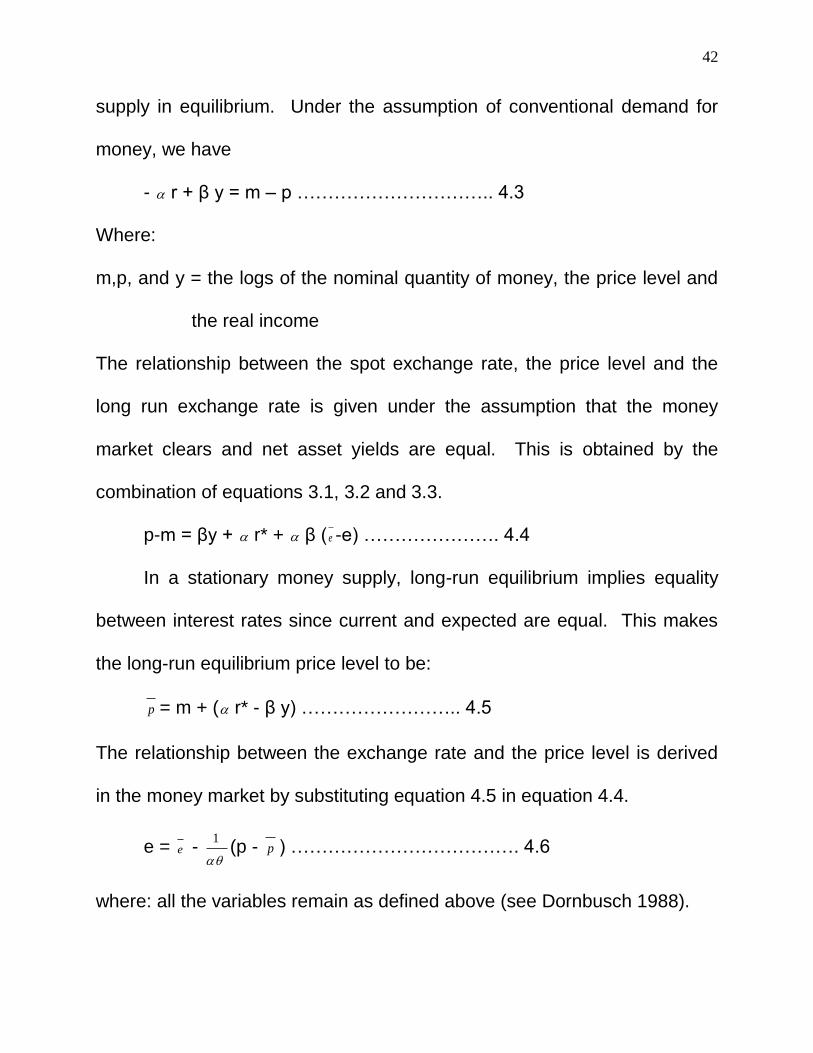
supply in equilibrium. Under the assumption of conventional demand for
money, we have
- r + β y = m – p ………………………….. 4.3
Where:
m,p, and y = the logs of the nominal quantity of money, the price level and
the real income
The relationship between the spot exchange rate, the price level and the
long run exchange rate is given under the assumption that the money
market clears and net asset yields are equal. This is obtained by the
combination of equations 3.1, 3.2 and 3.3.
p-m = βy + r* + β ( e -e) …………………. 4.4
In a stationary money supply, long-run equilibrium implies equality
between interest rates since current and expected are equal. This makes
the long-run equilibrium price level to be:
p = m + ( r* - β y) …………………….. 4.5
The relationship between the exchange rate and the price level is derived
in the money market by substituting equation 4.5 in equation 4.4.
e = e -
1(p - p ) ………………………………. 4.6
where: all the variables remain as defined above (see Dornbusch 1988).
43
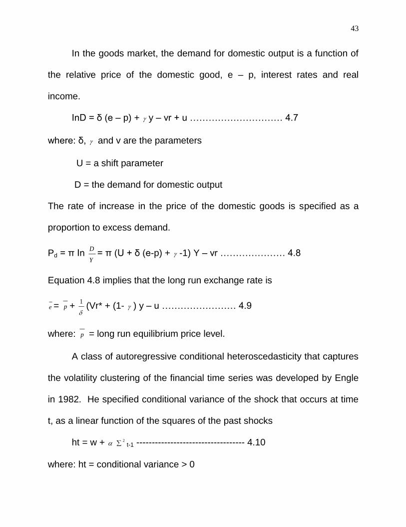
In the goods market, the demand for domestic output is a function of
the relative price of the domestic good, e – p, interest rates and real
income.
InD = δ (e – p) + y – vr + u ………………………… 4.7
where: δ, and v are the parameters
U = a shift parameter
D = the demand for domestic output
The rate of increase in the price of the domestic goods is specified as a
proportion to excess demand.
Pd = π In Y
D= π (U + δ (e-p) + -1) Y – vr ………………… 4.8
Equation 4.8 implies that the long run exchange rate is
e = p +
1(Vr* + (1- ) y – u …………………… 4.9
where: p = long run equilibrium price level.
A class of autoregressive conditional heteroscedasticity that captures
the volatility clustering of the financial time series was developed by Engle
in 1982. He specified conditional variance of the shock that occurs at time
t, as a linear function of the squares of the past shocks
ht = w + 2 t-1 ----------------------------------- 4.10
where: ht = conditional variance > 0
44
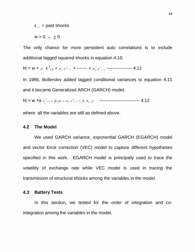
ε1t = past shocks
w > 0, 1
> 0
The only chance for more persistent auto correlations is to include
additional lagged squared shocks in equation 4.10.
ht = w + 1
ε 2
t-1 + 22
2 t + ------- + qtq 2
----------------- 4.11
In 1986, Bollerslev added lagged conditional variances to equation 4.11
and it became Generalized ARCH (GARCH) model.
ht = w +α )(212
2
111
2
1
ttt hw --------------------------- 4.12
where all the variables are still as defined above.
4.2 The Model
We used GARCH variance, exponential GARCH (EGARCH) model
and vector Error correction (VEC) model to capture different hypotheses
specified in this work. EGARCH model is principally used to trace the
volatility of exchange rate while VEC model is used in tracing the
transmission of structural shocks among the variables in the model.
4.3 Battery Tests
In this section, we tested for the order of integration and co-
integration among the variables in the model.
45
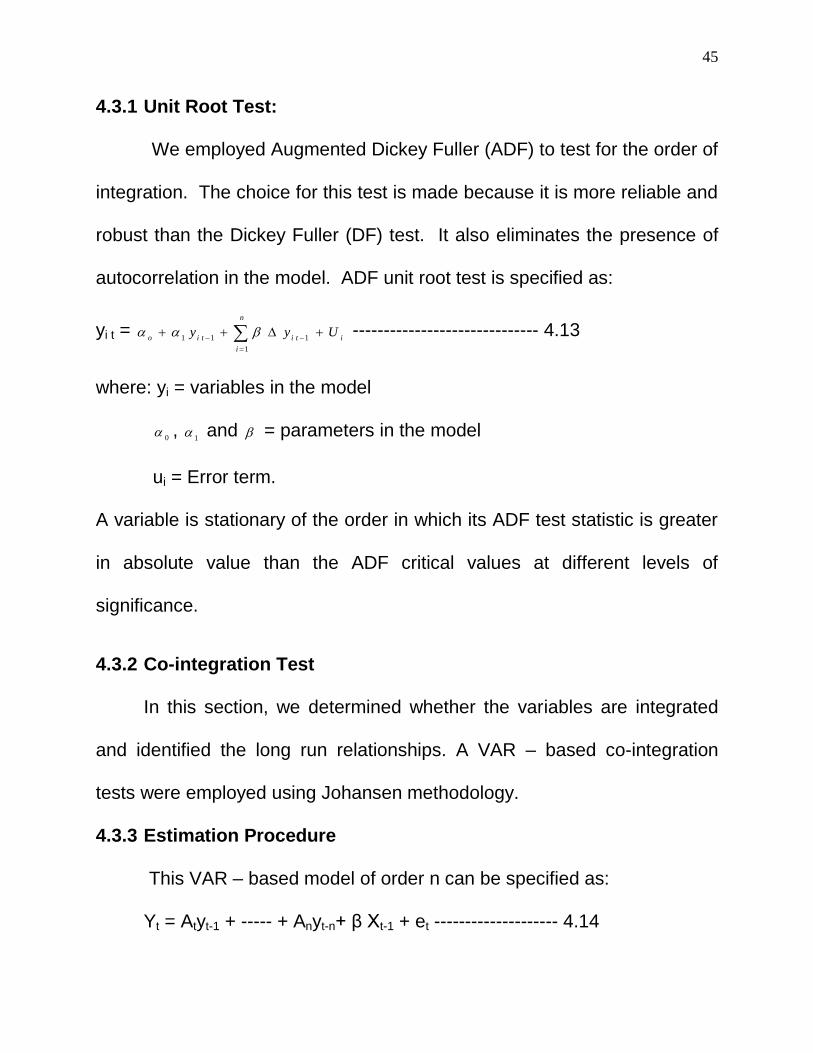
4.3.1 Unit Root Test:
We employed Augmented Dickey Fuller (ADF) to test for the order of
integration. The choice for this test is made because it is more reliable and
robust than the Dickey Fuller (DF) test. It also eliminates the presence of
autocorrelation in the model. ADF unit root test is specified as:
yi t = iti
n
i
tioUyy
1
1
11 ------------------------------ 4.13
where: yi = variables in the model
0
, 1
and = parameters in the model
ui = Error term.
A variable is stationary of the order in which its ADF test statistic is greater
in absolute value than the ADF critical values at different levels of
significance.
4.3.2 Co-integration Test
In this section, we determined whether the variables are integrated
and identified the long run relationships. A VAR – based co-integration
tests were employed using Johansen methodology.
4.3.3 Estimation Procedure
This VAR – based model of order n can be specified as:
Yt = Atyt-1 + ----- + Anyt-n+ β Xt-1 + et -------------------- 4.14
46
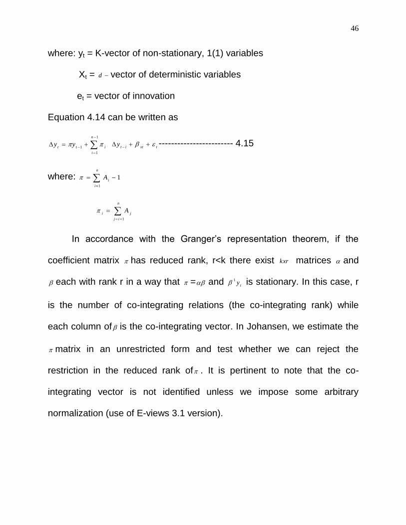
where: yt = K-vector of non-stationary, 1(1) variables
Xt = d vector of deterministic variables
et = vector of innovation
Equation 4.14 can be written as
1
1
1
n
i
ittyy
txtity
------------------------ 4.15
where: 1
1
n
i
iA
n
ij
jiA
1
In accordance with the Granger‟s representation theorem, if the
coefficient matrix has reduced rank, r<k there exist kxr matrices and
each with rank r in a way that = and t
y1
is stationary. In this case, r
is the number of co-integrating relations (the co-integrating rank) while
each column of is the co-integrating vector. In Johansen, we estimate the
matrix in an unrestricted form and test whether we can reject the
restriction in the reduced rank of . It is pertinent to note that the co-
integrating vector is not identified unless we impose some arbitrary
normalization (use of E-views 3.1 version).
47
4.4 Model Specification
4.4.1 Exponential GARCH Model
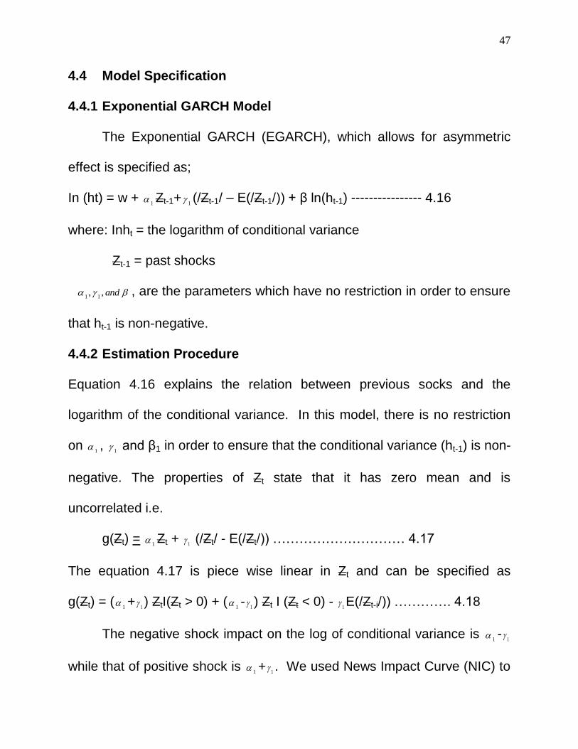
The Exponential GARCH (EGARCH), which allows for asymmetric
effect is specified as;
In (ht) = w + 1
Zt-1+ 1 (/Zt-1/ – E(/Zt-1/)) + β ln(ht-1) ---------------- 4.16
where: Inht = the logarithm of conditional variance
Zt-1 = past shocks
and,,11
, are the parameters which have no restriction in order to ensure
that ht-1 is non-negative.
4.4.2 Estimation Procedure
Equation 4.16 explains the relation between previous socks and the
logarithm of the conditional variance. In this model, there is no restriction
on 1
, 1
and β1 in order to ensure that the conditional variance (ht-1) is non-
negative. The properties of Zt state that it has zero mean and is
uncorrelated i.e.
g(Zt) = 1
Zt + 1
(/Zt/ - E(/Zt/)) ………………………… 4.17
The equation 4.17 is piece wise linear in Zt and can be specified as
g(Zt) = (1
+1
) ZtI(Zt > 0) + (1
-1
) Zt I (Zt < 0) - 1
E(/Zt-i/)) …………. 4.18
The negative shock impact on the log of conditional variance is 1
-1
while that of positive shock is 1
+1
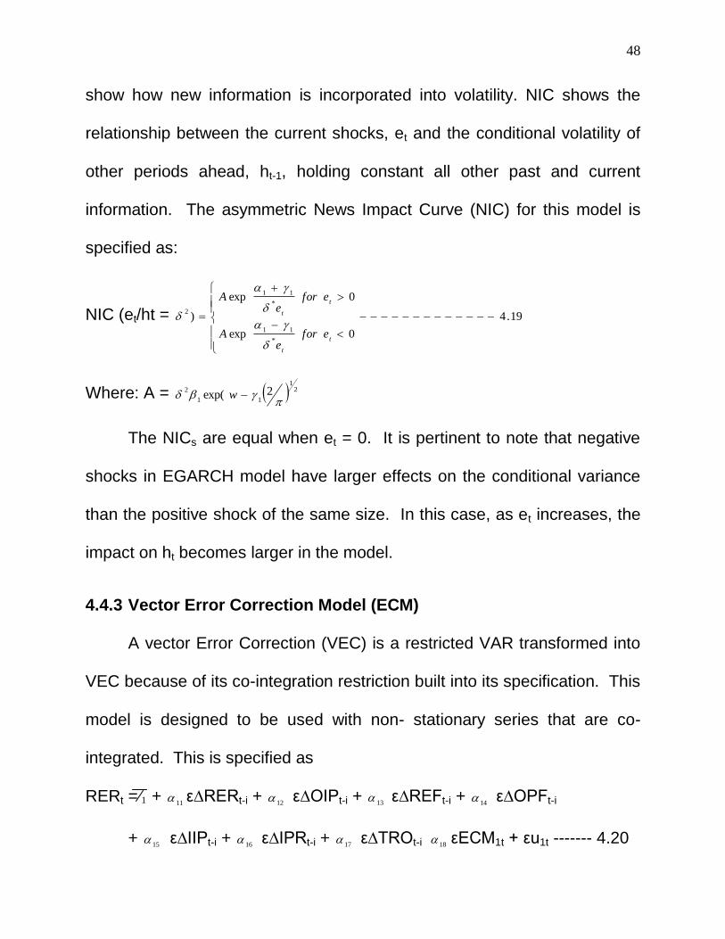
. We used News Impact Curve (NIC) to
48
show how new information is incorporated into volatility. NIC shows the
relationship between the current shocks, et and the conditional volatility of
other periods ahead, ht-1, holding constant all other past and current
information. The asymmetric News Impact Curve (NIC) for this model is
specified as:
NIC (et/ht = 19.4
0exp
0exp
)
*
11
*
11
2
t
t
t
t
efore
A
efore
A
Where: A = 21
11
2 2exp(
w
The NICs are equal when et = 0. It is pertinent to note that negative
shocks in EGARCH model have larger effects on the conditional variance
than the positive shock of the same size. In this case, as et increases, the
impact on ht becomes larger in the model.
4.4.3 Vector Error Correction Model (ECM)
A vector Error Correction (VEC) is a restricted VAR transformed into
VEC because of its co-integration restriction built into its specification. This
model is designed to be used with non- stationary series that are co-
integrated. This is specified as
RERt = + 11
ε∆RERt-i + 12
ε∆OIPt-i + 13
ε∆REFt-i + 14
ε∆OPFt-i
+ 15
ε∆IIPt-i + 16
ε∆IPRt-i + 17
ε∆TROt-i 18 εECM1t + εu1t ------- 4.20
1
49
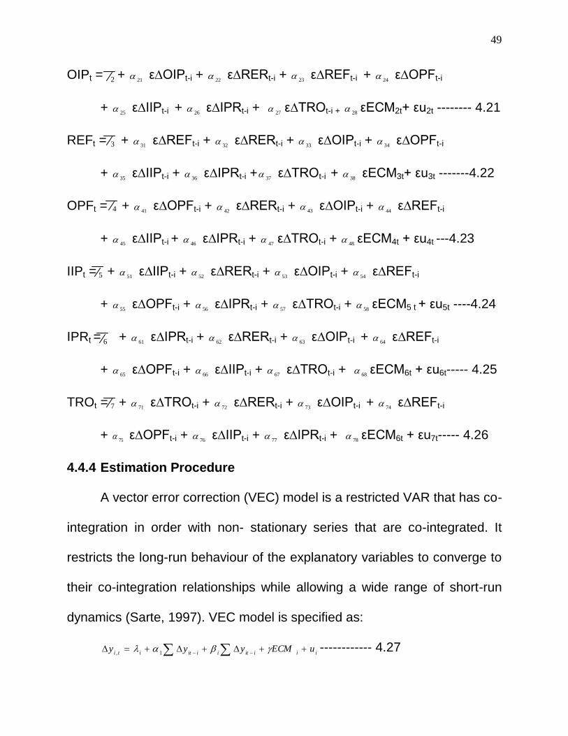
OIPt = + 21
ε∆OIPt-i + 22
ε∆RERt-i + 23
ε∆REFt-i + 24
ε∆OPFt-i
+ 25
ε∆IIPt-i + 26
ε∆IPRt-i + 27
ε∆TROt-i + 28 εECM2t+ εu2t -------- 4.21
REFt = + 31
ε∆REFt-i + 32
ε∆RERt-i + 33
ε∆OIPt-i + 34
ε∆OPFt-i
+ 35
ε∆IIPt-i + 36
ε∆IPRt-i + 37 ε∆TROt-i +
38 εECM3t+ εu3t -------4.22
OPFt = + 41
ε∆OPFt-i + 42
ε∆RERt-i + 43
ε∆OIPt-i + 44
ε∆REFt-i
+ 45
ε∆IIPt-i + 46
ε∆IPRt-i + 47
ε∆TROt-i + 48
εECM4t + εu4t ---4.23
IIPt = + 51
ε∆IIPt-i + 52
ε∆RERt-i + 53
ε∆OIPt-i + 54
ε∆REFt-i
+ 55
ε∆OPFt-i + 56
ε∆IPRt-i + 57
ε∆TROt-i + 58
εECM5 t + εu5t ----4.24
IPRt = + 61
ε∆IPRt-i + 62
ε∆RERt-i + 63
ε∆OIPt-i + 64
ε∆REFt-i
+ 65
ε∆OPFt-i + 66
ε∆IIPt-i + 67
ε∆TROt-i + 68
εECM6t + εu6t----- 4.25
TROt = + 71
ε∆TROt-i + 72
ε∆RERt-i + 73
ε∆OIPt-i + 74
ε∆REFt-i
+ 75
ε∆OPFt-i + 76
ε∆IIPt-i + 77
ε∆IPRt-i + 78
εECM6t + εu7t----- 4.26
4.4.4 Estimation Procedure
A vector error correction (VEC) model is a restricted VAR that has co-
integration in order with non- stationary series that are co-integrated. It
restricts the long-run behaviour of the explanatory variables to converge to
their co-integration relationships while allowing a wide range of short-run
dynamics (Sarte, 1997). VEC model is specified as:
iiiitiiititiuECMyyy
1,
------------ 4.27
2
3
4
5
6
7
50
where:
iy = change in individual variable in the model.
72,1
i
7722,21,1211,,,
i= parameters in the model.
1ity = lagged variables in the model
iu = Random innovations
= error correction parameter
ECM = Error correction term
(Davidson and Mackinnon 1993, Hamilton 1994, Sarte 1997)
Where: RER = real exchange rate
OIP = international oil price
REF = real exchange rate fluctuations
OPF = international oil price fluctuations
IIP = index of industrial production (as a proxy to GDP)
IPR = industrial production growth rate
TRO = GDP
MX
X = Export
M = Import
51
ECMs = Error correction terms which are generated from the co-
integrating residuals.
We call the co-integration term an error correction term because the
deviation from the long run equilibrium is gradually corrected through a
series of partial short-run adjustment. (See, Amin and Awung 1997, Parikh
1997, Cooley and Leroy 1985, Sarte 1997)
4.4.5 Justification of the Models
We employed Augmented Dickey Fuller (ADF) test statistic to test the
order of integration. The choice of this test was made because it is more
reliable and robust than the Dickey Fuller (DF) test. It also eliminates the
presence of autocorrelation in the model.
The co-integration test was employed to determine whether the
variables are integrated and to identify the long-run relationships in the
variables. Knowing the number of co-integrating vectors will help us run the
vector error correction. The number of the co-integrating vectors so
identified becomes the number of restrictions placed on VAR to run the
VEC.
We equally, employed the EGARCH model to trace the volatility of
the dependent variable. This model allows for asymmetric effects. It shows
52
the relationship between past shocks and the logarithm of the conditional
variance.
The vector error correction (VEC) model was employed because it
restricts the long-run behaviour of the explanatory variables to converge to
their co-integration relationships while allowing a wide range of short-run
dynamics.
4.5 Package for Estimation
The models were estimated with the aid of E-view Econometric
package with OLS technique. The OLS technique is chosen because it
gives us the best linear unbiased estimates while the package is a user -
friendly computer application that handles time series data efficiently.
4.6 Data
Data for this study were obtained from the CBN statistical Bulletin and
the annual publications of the National Bureau of statistic (NBS) of various
years.
4.7 Estimation of Variables
The data on the following variables Real Exchange Rate (RER), real
exchange rate fluctuation (REF), index of industrial production (IIP), and
industrial production growth rate (IPR) were based on the values as given
53
by the CBN statistical Bulletin and the annual publications of the National
Bureau of statistic (NBS) of various years. This is because they are
already transformed time series data. The data on trade Openness (TRO)
was estimated by GDP
MX
where: X = Export
M = Import
GDP = Gross domestic product
The data on oil price (OIP) and oil price fluctuations (OPF) were
estimated by changes in international crude oil prices in domestic currency.
We collected annual time series data on the variables from 1986-
2008. To avoid sample errors because of the small sample size, 1986-2008
is only 23years, we used interpolation package to transform the data into
quarterly data.
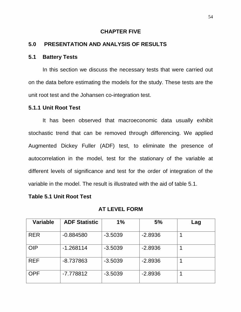
54
CHAPTER FIVE
5.0 PRESENTATION AND ANALYSIS OF RESULTS
5.1 Battery Tests
In this section we discuss the necessary tests that were carried out
on the data before estimating the models for the study. These tests are the
unit root test and the Johansen co-integration test.
5.1.1 Unit Root Test
It has been observed that macroeconomic data usually exhibit
stochastic trend that can be removed through differencing. We applied
Augmented Dickey Fuller (ADF) test, to eliminate the presence of
autocorrelation in the model, test for the stationary of the variable at
different levels of significance and test for the order of integration of the
variable in the model. The result is illustrated with the aid of table 5.1.
Table 5.1 Unit Root Test
AT LEVEL FORM
Variable ADF Statistic 1% 5% Lag
RER -0.884580 -3.5039 -2.8936 1
OIP -1.268114 -3.5039 -2.8936 1
REF -8.737863 -3.5039 -2.8936 1
OPF -7.778812 -3.5039 -2.8936 1
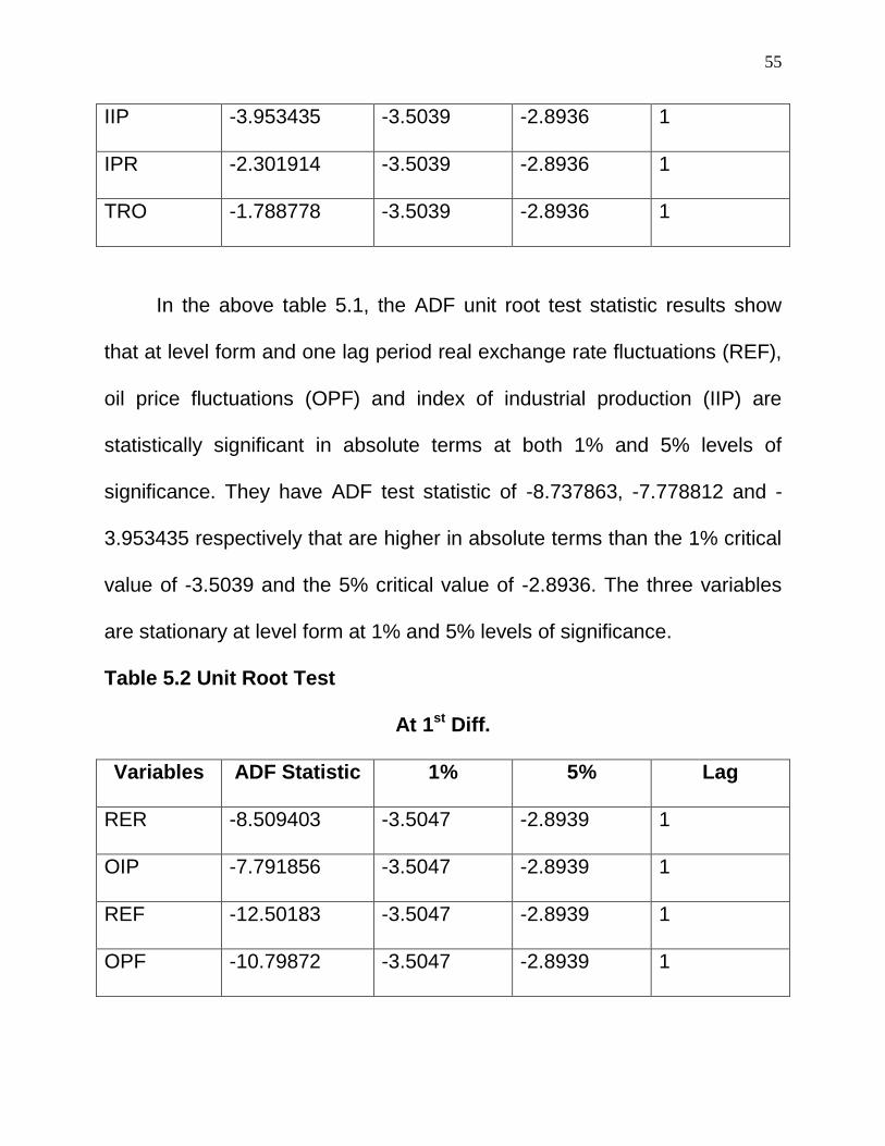
55
IIP -3.953435 -3.5039 -2.8936 1
IPR -2.301914 -3.5039 -2.8936 1
TRO -1.788778 -3.5039 -2.8936 1
In the above table 5.1, the ADF unit root test statistic results show
that at level form and one lag period real exchange rate fluctuations (REF),
oil price fluctuations (OPF) and index of industrial production (IIP) are
statistically significant in absolute terms at both 1% and 5% levels of
significance. They have ADF test statistic of -8.737863, -7.778812 and -
3.953435 respectively that are higher in absolute terms than the 1% critical
value of -3.5039 and the 5% critical value of -2.8936. The three variables
are stationary at level form at 1% and 5% levels of significance.
Table 5.2 Unit Root Test
At 1st Diff.
Variables ADF Statistic 1% 5% Lag
RER -8.509403 -3.5047 -2.8939 1
OIP -7.791856 -3.5047 -2.8939 1
REF -12.50183 -3.5047 -2.8939 1
OPF -10.79872 -3.5047 -2.8939 1
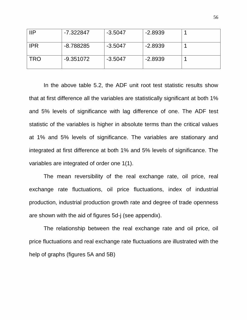
56
IIP -7.322847 -3.5047 -2.8939 1
IPR -8.788285 -3.5047 -2.8939 1
TRO -9.351072 -3.5047 -2.8939 1
In the above table 5.2, the ADF unit root test statistic results show
that at first difference all the variables are statistically significant at both 1%
and 5% levels of significance with lag difference of one. The ADF test
statistic of the variables is higher in absolute terms than the critical values
at 1% and 5% levels of significance. The variables are stationary and
integrated at first difference at both 1% and 5% levels of significance. The
variables are integrated of order one 1(1).
The mean reversibility of the real exchange rate, oil price, real
exchange rate fluctuations, oil price fluctuations, index of industrial
production, industrial production growth rate and degree of trade openness
are shown with the aid of figures 5d-j (see appendix).
The relationship between the real exchange rate and oil price, oil
price fluctuations and real exchange rate fluctuations are illustrated with the
help of graphs (figures 5A and 5B)
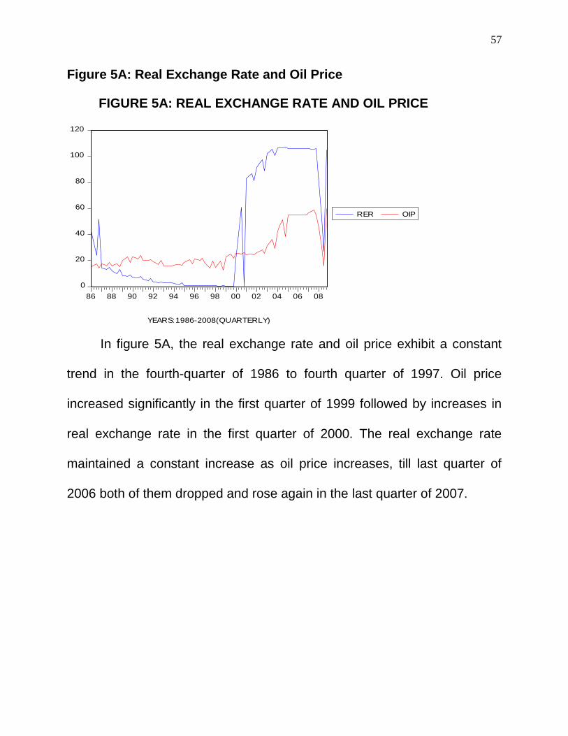
57
Figure 5A: Real Exchange Rate and Oil Price
In figure 5A, the real exchange rate and oil price exhibit a constant
trend in the fourth-quarter of 1986 to fourth quarter of 1997. Oil price
increased significantly in the first quarter of 1999 followed by increases in
real exchange rate in the first quarter of 2000. The real exchange rate
maintained a constant increase as oil price increases, till last quarter of
2006 both of them dropped and rose again in the last quarter of 2007.
0
20
40
60
80
100
120
86 88 90 92 94 96 98 00 02 04 06 08
RER OIP
FIGURE 5H: REAL EXCHANGE RATE AND OIL PRICE
YEARS: 1986-2008(QUARTERLY)
FIGURE 5A: REAL EXCHANGE RATE AND OIL PRICE
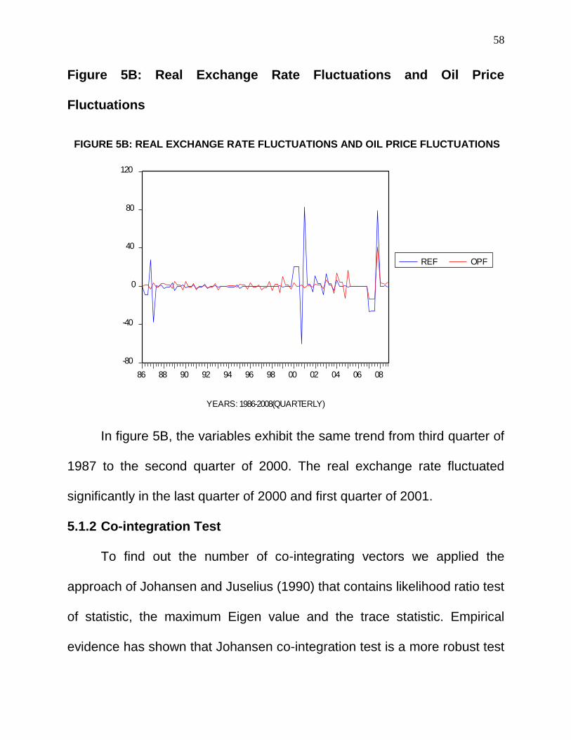
58
Figure 5B: Real Exchange Rate Fluctuations and Oil Price
Fluctuations
In figure 5B, the variables exhibit the same trend from third quarter of
1987 to the second quarter of 2000. The real exchange rate fluctuated
significantly in the last quarter of 2000 and first quarter of 2001.
5.1.2 Co-integration Test
To find out the number of co-integrating vectors we applied the
approach of Johansen and Juselius (1990) that contains likelihood ratio test
of statistic, the maximum Eigen value and the trace statistic. Empirical
evidence has shown that Johansen co-integration test is a more robust test
-80
-40
0
40
80
120
86 88 90 92 94 96 98 00 02 04 06 08
REF OPF
FIGURE 5I: REAL EXCHANGE RATE FLUCTUATIONS AND OIL PRICE FLUCTUATIONS
YEARS: 1986-2008(QUARTERLY)
FIGURE 5B: REAL EXCHANGE RATE FLUCTUATIONS AND OIL PRICE FLUCTUATIONS
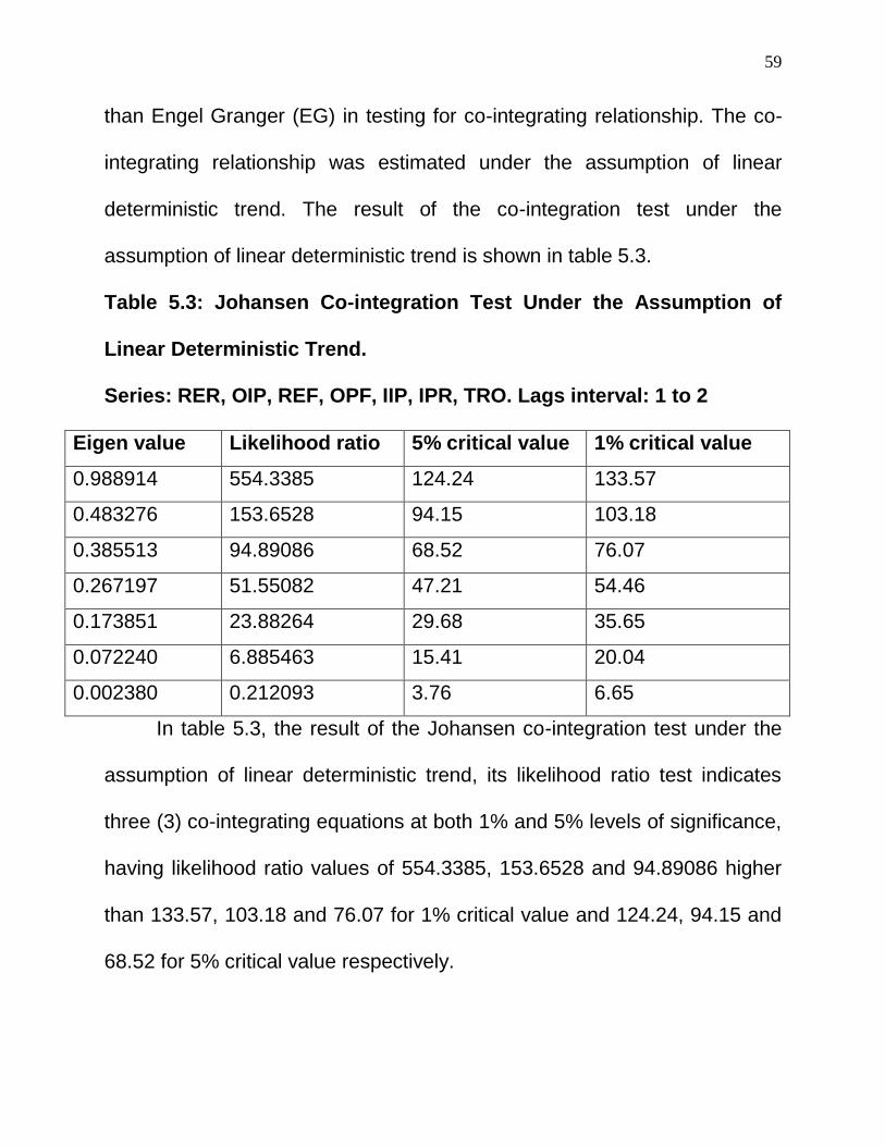
59
than Engel Granger (EG) in testing for co-integrating relationship. The co-
integrating relationship was estimated under the assumption of linear
deterministic trend. The result of the co-integration test under the
assumption of linear deterministic trend is shown in table 5.3.
Table 5.3: Johansen Co-integration Test Under the Assumption of
Linear Deterministic Trend.
Series: RER, OIP, REF, OPF, IIP, IPR, TRO. Lags interval: 1 to 2
Eigen value Likelihood ratio 5% critical value 1% critical value
0.988914 554.3385 124.24 133.57
0.483276 153.6528 94.15 103.18
0.385513 94.89086 68.52 76.07
0.267197 51.55082 47.21 54.46
0.173851 23.88264 29.68 35.65
0.072240 6.885463 15.41 20.04
0.002380 0.212093 3.76 6.65
In table 5.3, the result of the Johansen co-integration test under the
assumption of linear deterministic trend, its likelihood ratio test indicates
three (3) co-integrating equations at both 1% and 5% levels of significance,
having likelihood ratio values of 554.3385, 153.6528 and 94.89086 higher
than 133.57, 103.18 and 76.07 for 1% critical value and 124.24, 94.15 and
68.52 for 5% critical value respectively.
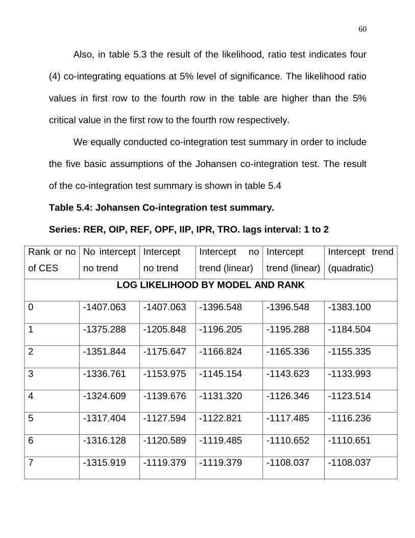
60
Also, in table 5.3 the result of the likelihood, ratio test indicates four
(4) co-integrating equations at 5% level of significance. The likelihood ratio
values in first row to the fourth row in the table are higher than the 5%
critical value in the first row to the fourth row respectively.
We equally conducted co-integration test summary in order to include
the five basic assumptions of the Johansen co-integration test. The result
of the co-integration test summary is shown in table 5.4
Table 5.4: Johansen Co-integration test summary.
Series: RER, OIP, REF, OPF, IIP, IPR, TRO. lags interval: 1 to 2
Rank or no
of CES
No intercept
no trend
Intercept
no trend
Intercept no
trend (linear)
Intercept
trend (linear)
Intercept trend
(quadratic)
LOG LIKELIHOOD BY MODEL AND RANK
0 -1407.063 -1407.063 -1396.548 -1396.548 -1383.100
1 -1375.288 -1205.848 -1196.205 -1195.288 -1184.504
2 -1351.844 -1175.647 -1166.824 -1165.336 -1155.335
3 -1336.761 -1153.975 -1145.154 -1143.623 -1133.993
4 -1324.609 -1139.676 -1131.320 -1126.346 -1123.514
5 -1317.404 -1127.594 -1122.821 -1117.485 -1116.236
6 -1316.128 -1120.589 -1119.485 -1110.652 -1110.651
7 -1315.919 -1119.379 -1119.379 -1108.037 -1108.037
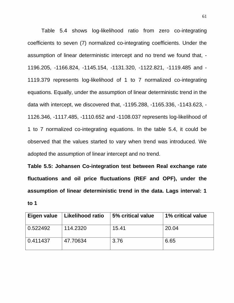
61
Table 5.4 shows log-likelihood ratio from zero co-integrating
coefficients to seven (7) normalized co-integrating coefficients. Under the
assumption of linear deterministic intercept and no trend we found that, -
1196.205, -1166.824, -1145.154, -1131.320, -1122.821, -1119.485 and -
1119.379 represents log-likelihood of 1 to 7 normalized co-integrating
equations. Equally, under the assumption of linear deterministic trend in the
data with intercept, we discovered that, -1195.288, -1165.336, -1143.623, -
1126.346, -1117.485, -1110.652 and -1108.037 represents log-likelihood of
1 to 7 normalized co-integrating equations. In the table 5.4, it could be
observed that the values started to vary when trend was introduced. We
adopted the assumption of linear intercept and no trend.
Table 5.5: Johansen Co-integration test between Real exchange rate
fluctuations and oil price fluctuations (REF and OPF), under the
assumption of linear deterministic trend in the data. Lags interval: 1
to 1
Eigen value Likelihood ratio 5% critical value 1% critical value
0.522492 114.2320 15.41 20.04
0.411437 47.70634 3.76 6.65
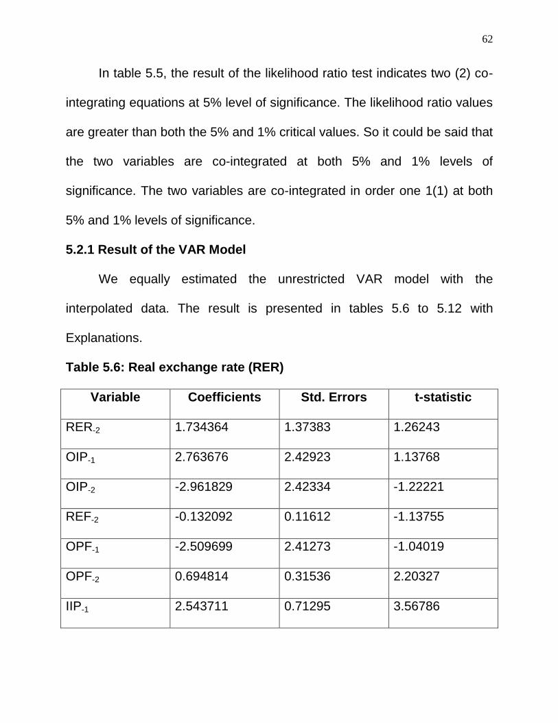
62
In table 5.5, the result of the likelihood ratio test indicates two (2) co-
integrating equations at 5% level of significance. The likelihood ratio values
are greater than both the 5% and 1% critical values. So it could be said that
the two variables are co-integrated at both 5% and 1% levels of
significance. The two variables are co-integrated in order one 1(1) at both
5% and 1% levels of significance.
5.2.1 Result of the VAR Model
We equally estimated the unrestricted VAR model with the
interpolated data. The result is presented in tables 5.6 to 5.12 with
Explanations.
Table 5.6: Real exchange rate (RER)
Variable Coefficients Std. Errors t-statistic
RER-2 1.734364 1.37383 1.26243
OIP-1 2.763676 2.42923 1.13768
OIP-2 -2.961829 2.42334 -1.22221
REF-2 -0.132092 0.11612 -1.13755
OPF-1 -2.509699 2.41273 -1.04019
OPF-2 0.694814 0.31536 2.20327
IIP-1 2.543711 0.71295 3.56786
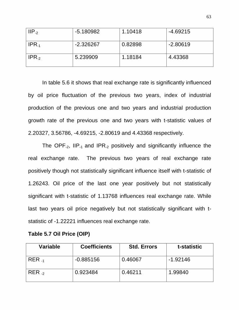
63
IIP-2 -5.180982 1.10418 -4.69215
IPR-1 -2.326267 0.82898 -2.80619
IPR-2 5.239909 1.18184 4.43368
In table 5.6 it shows that real exchange rate is significantly influenced
by oil price fluctuation of the previous two years, index of industrial
production of the previous one and two years and industrial production
growth rate of the previous one and two years with t-statistic values of
2.20327, 3.56786, -4.69215, -2.80619 and 4.43368 respectively.
The OPF-2, IIP-1 and IPR-2 positively and significantly influence the
real exchange rate. The previous two years of real exchange rate
positively though not statistically significant influence itself with t-statistic of
1.26243. Oil price of the last one year positively but not statistically
significant with t-statistic of 1.13768 influences real exchange rate. While
last two years oil price negatively but not statistically significant with t-
statistic of -1.22221 influences real exchange rate.
Table 5.7 Oil Price (OIP)
Variable Coefficients Std. Errors t-statistic
RER -1 -0.885156 0.46067 -1.92146
RER -2 0.923484 0.46211 1.99840
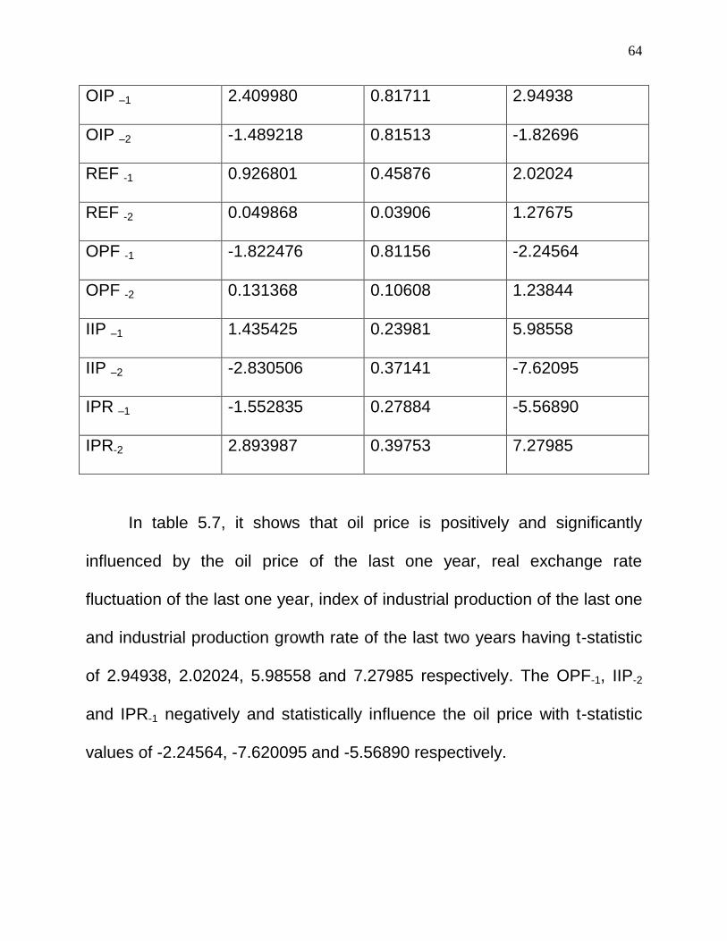
64
OIP –1 2.409980 0.81711 2.94938
OIP –2 -1.489218 0.81513 -1.82696
REF -1 0.926801 0.45876 2.02024
REF -2 0.049868 0.03906 1.27675
OPF -1 -1.822476 0.81156 -2.24564
OPF -2 0.131368 0.10608 1.23844
IIP –1 1.435425 0.23981 5.98558
IIP –2 -2.830506 0.37141 -7.62095
IPR –1 -1.552835 0.27884 -5.56890
IPR-2 2.893987 0.39753 7.27985
In table 5.7, it shows that oil price is positively and significantly
influenced by the oil price of the last one year, real exchange rate
fluctuation of the last one year, index of industrial production of the last one
and industrial production growth rate of the last two years having t-statistic
of 2.94938, 2.02024, 5.98558 and 7.27985 respectively. The OPF-1, IIP-2
and IPR-1 negatively and statistically influence the oil price with t-statistic
values of -2.24564, -7.620095 and -5.56890 respectively.
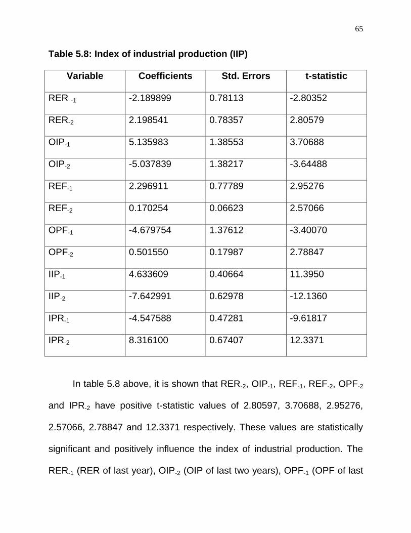
65
Table 5.8: Index of industrial production (IIP)
Variable Coefficients Std. Errors t-statistic
RER -1 -2.189899 0.78113 -2.80352
RER-2 2.198541 0.78357 2.80579
OIP-1 5.135983 1.38553 3.70688
OIP-2 -5.037839 1.38217 -3.64488
REF-1 2.296911 0.77789 2.95276
REF-2 0.170254 0.06623 2.57066
OPF-1 -4.679754 1.37612 -3.40070
OPF-2 0.501550 0.17987 2.78847
IIP-1 4.633609 0.40664 11.3950
IIP-2 -7.642991 0.62978 -12.1360
IPR-1 -4.547588 0.47281 -9.61817
IPR-2 8.316100 0.67407 12.3371
In table 5.8 above, it is shown that RER-2, OIP-1, REF-1, REF-2, OPF-2
and IPR-2 have positive t-statistic values of 2.80597, 3.70688, 2.95276,
2.57066, 2.78847 and 12.3371 respectively. These values are statistically
significant and positively influence the index of industrial production. The
RER-1 (RER of last year), OIP-2 (OIP of last two years), OPF-1 (OPF of last
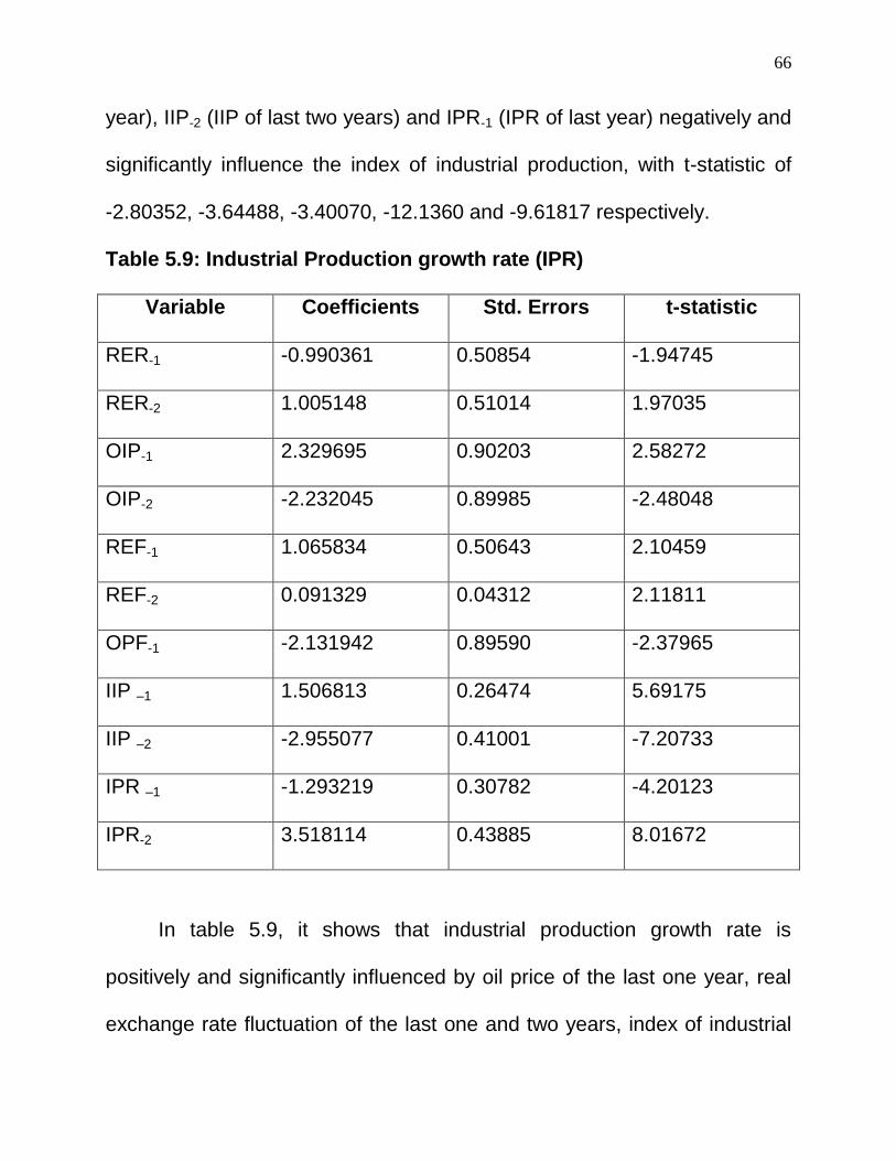
66
year), IIP-2 (IIP of last two years) and IPR-1 (IPR of last year) negatively and
significantly influence the index of industrial production, with t-statistic of
-2.80352, -3.64488, -3.40070, -12.1360 and -9.61817 respectively.
Table 5.9: Industrial Production growth rate (IPR)
Variable Coefficients Std. Errors t-statistic
RER-1 -0.990361 0.50854 -1.94745
RER-2 1.005148 0.51014 1.97035
OIP-1 2.329695 0.90203 2.58272
OIP-2 -2.232045 0.89985 -2.48048
REF-1 1.065834 0.50643 2.10459
REF-2 0.091329 0.04312 2.11811
OPF-1 -2.131942 0.89590 -2.37965
IIP –1 1.506813 0.26474 5.69175
IIP –2 -2.955077 0.41001 -7.20733
IPR –1 -1.293219 0.30782 -4.20123
IPR-2 3.518114 0.43885 8.01672
In table 5.9, it shows that industrial production growth rate is
positively and significantly influenced by oil price of the last one year, real
exchange rate fluctuation of the last one and two years, index of industrial

67
production of the last one year and by itself of the last two years, having
t-statistic values of 2.58272, 2.10459, 2.11811, 5.69175 and 8.01672
respectively. On the other hand the oil price of the last two years, oil price
fluctuations of the last year, index of industrial production of the last two
years and industrial production growth rate of the last year negatively and
significantly influence the industrial production growth rate with t-statistic
values of -2.48048, -2.37965, -7.20733 and -4.20123 respectively.
Table 5.10: Degree of trade openness (TRO)
Variable Coefficients Std. Errors t-statistic
RER -1 0.011603 0.01053 1.10167
RER -2 -0.010970 0.01057 -1.03826
OIP –1 -0.029235 0.01868 -1.56488
OIP –2 0.030355 0.01864 1.62876
REF -1 -0.011947 0.01049 -1.13899
REF -2 -0.000896 0.00089 -1.00336
OPF -1 0.024557 0.01856 1.32348
OPF -2 -0.004022 0.00243 -1.65840
IIP –1 -0.024113 0.00548 -4.39787
IIP –2 0.049153 0.00849 5.78832
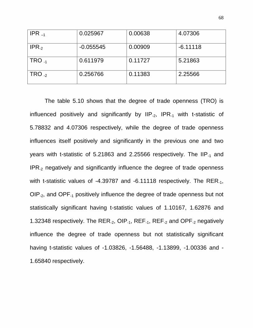
68
IPR –1 0.025967 0.00638 4.07306
IPR-2 -0.055545 0.00909 -6.11118
TRO -1 0.611979 0.11727 5.21863
TRO -2 0.256766 0.11383 2.25566
The table 5.10 shows that the degree of trade openness (TRO) is
influenced positively and significantly by IIP-2, IPR-1 with t-statistic of
5.78832 and 4.07306 respectively, while the degree of trade openness
influences itself positively and significantly in the previous one and two
years with t-statistic of 5.21863 and 2.25566 respectively. The IIP-1 and
IPR-2 negatively and significantly influence the degree of trade openness
with t-statistic values of -4.39787 and -6.11118 respectively. The RER-1,
OIP-2, and OPF-1 positively influence the degree of trade openness but not
statistically significant having t-statistic values of 1.10167, 1.62876 and
1.32348 respectively. The RER-2, OIP-1, REF-1, REF-2 and OPF-2 negatively
influence the degree of trade openness but not statistically significant
having t-statistic values of -1.03826, -1.56488, -1.13899, -1.00336 and -
1.65840 respectively.
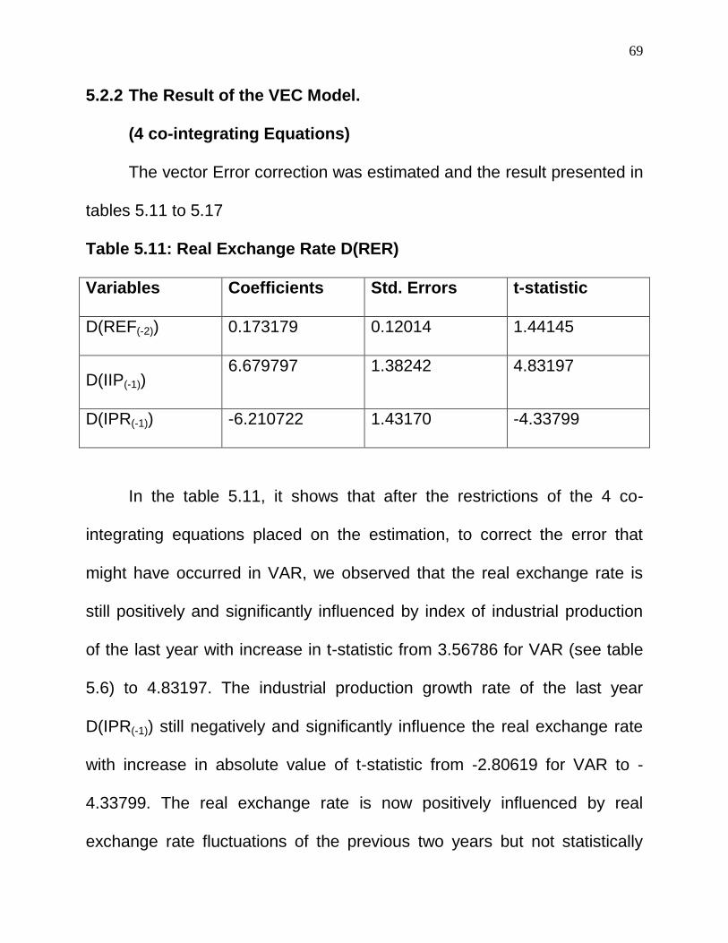
69
5.2.2 The Result of the VEC Model.
(4 co-integrating Equations)
The vector Error correction was estimated and the result presented in
tables 5.11 to 5.17
Table 5.11: Real Exchange Rate D(RER)
Variables Coefficients Std. Errors t-statistic
D(REF(-2)) 0.173179 0.12014 1.44145
D(IIP(-1)) 6.679797 1.38242 4.83197
D(IPR(-1)) -6.210722 1.43170 -4.33799
In the table 5.11, it shows that after the restrictions of the 4 co-
integrating equations placed on the estimation, to correct the error that
might have occurred in VAR, we observed that the real exchange rate is
still positively and significantly influenced by index of industrial production
of the last year with increase in t-statistic from 3.56786 for VAR (see table
5.6) to 4.83197. The industrial production growth rate of the last year
D(IPR(-1)) still negatively and significantly influence the real exchange rate
with increase in absolute value of t-statistic from -2.80619 for VAR to -
4.33799. The real exchange rate is now positively influenced by real
exchange rate fluctuations of the previous two years but not statistically
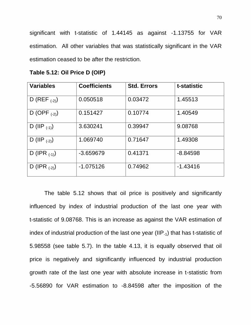
70
significant with t-statistic of 1.44145 as against -1.13755 for VAR
estimation. All other variables that was statistically significant in the VAR
estimation ceased to be after the restriction.
Table 5.12: Oil Price D (OIP)
Variables Coefficients Std. Errors t-statistic
D (REF (-2)) 0.050518 0.03472 1.45513
D (OPF (-2)) 0.151427 0.10774 1.40549
D (IIP (-1)) 3.630241 0.39947 9.08768
D (IIP (-2)) 1.069740 0.71647 1.49308
D (IPR (-1)) -3.659679 0.41371 -8.84598
D (IPR (-2)) -1.075126 0.74962 -1.43416
The table 5.12 shows that oil price is positively and significantly
influenced by index of industrial production of the last one year with
t-statistic of 9.08768. This is an increase as against the VAR estimation of
index of industrial production of the last one year (IIP-1) that has t-statistic of
5.98558 (see table 5.7). In the table 4.13, it is equally observed that oil
price is negatively and significantly influenced by industrial production
growth rate of the last one year with absolute increase in t-statistic from
-5.56890 for VAR estimation to -8.84598 after the imposition of the
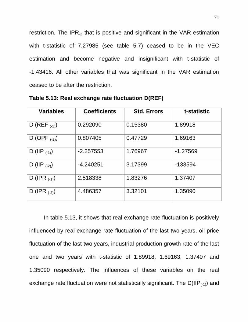
71
restriction. The IPR-2 that is positive and significant in the VAR estimation
with t-statistic of 7.27985 (see table 5.7) ceased to be in the VEC
estimation and become negative and insignificant with t-statistic of
-1.43416. All other variables that was significant in the VAR estimation
ceased to be after the restriction.
Table 5.13: Real exchange rate fluctuation D(REF)
Variables Coefficients Std. Errors t-statistic
D (REF (-2)) 0.292090 0.15380 1.89918
D (OPF (-2)) 0.807405 0.47729 1.69163
D (IIP (-1)) -2.257553 1.76967 -1.27569
D (IIP (-2)) -4.240251 3.17399 -133594
D (IPR (-1)) 2.518338 1.83276 1.37407
D (IPR (-2)) 4.486357 3.32101 1.35090
In table 5.13, it shows that real exchange rate fluctuation is positively
influenced by real exchange rate fluctuation of the last two years, oil price
fluctuation of the last two years, industrial production growth rate of the last
one and two years with t-statistic of 1.89918, 1.69163, 1.37407 and
1.35090 respectively. The influences of these variables on the real
exchange rate fluctuation were not statistically significant. The D(IIP(-1)) and
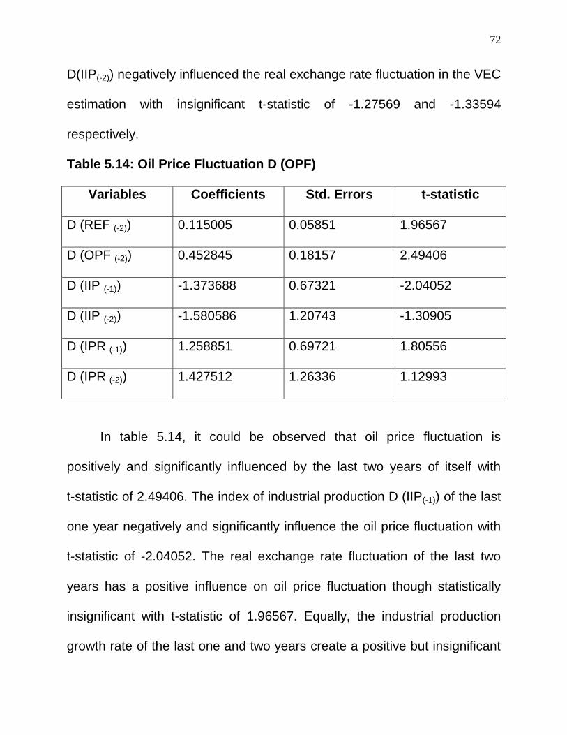
72
D(IIP(-2)) negatively influenced the real exchange rate fluctuation in the VEC
estimation with insignificant t-statistic of -1.27569 and -1.33594
respectively.
Table 5.14: Oil Price Fluctuation D (OPF)
Variables Coefficients Std. Errors t-statistic
D (REF (-2)) 0.115005 0.05851 1.96567
D (OPF (-2)) 0.452845 0.18157 2.49406
D (IIP (-1)) -1.373688 0.67321 -2.04052
D (IIP (-2)) -1.580586 1.20743 -1.30905
D (IPR (-1)) 1.258851 0.69721 1.80556
D (IPR (-2)) 1.427512 1.26336 1.12993
In table 5.14, it could be observed that oil price fluctuation is
positively and significantly influenced by the last two years of itself with
t-statistic of 2.49406. The index of industrial production D (IIP(-1)) of the last
one year negatively and significantly influence the oil price fluctuation with
t-statistic of -2.04052. The real exchange rate fluctuation of the last two
years has a positive influence on oil price fluctuation though statistically
insignificant with t-statistic of 1.96567. Equally, the industrial production
growth rate of the last one and two years create a positive but insignificant
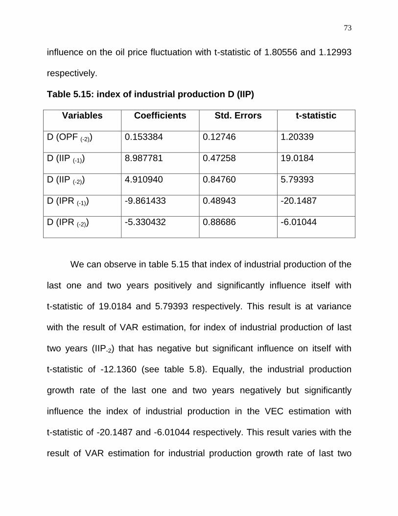
73
influence on the oil price fluctuation with t-statistic of 1.80556 and 1.12993
respectively.
Table 5.15: index of industrial production D (IIP)
Variables Coefficients Std. Errors t-statistic
D (OPF (-2)) 0.153384 0.12746 1.20339
D (IIP (-1)) 8.987781 0.47258 19.0184
D (IIP (-2)) 4.910940 0.84760 5.79393
D (IPR (-1)) -9.861433 0.48943 -20.1487
D (IPR (-2)) -5.330432 0.88686 -6.01044
We can observe in table 5.15 that index of industrial production of the
last one and two years positively and significantly influence itself with
t-statistic of 19.0184 and 5.79393 respectively. This result is at variance
with the result of VAR estimation, for index of industrial production of last
two years (IIP-2) that has negative but significant influence on itself with
t-statistic of -12.1360 (see table 5.8). Equally, the industrial production
growth rate of the last one and two years negatively but significantly
influence the index of industrial production in the VEC estimation with
t-statistic of -20.1487 and -6.01044 respectively. This result varies with the
result of VAR estimation for industrial production growth rate of last two
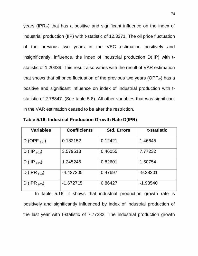
74
years (IPR-2) that has a positive and significant influence on the index of
industrial production (IIP) with t-statistic of 12.3371. The oil price fluctuation
of the previous two years in the VEC estimation positively and
insignificantly, influence, the index of industrial production D(IIP) with t-
statistic of 1.20339. This result also varies with the result of VAR estimation
that shows that oil price fluctuation of the previous two years (OPF-2) has a
positive and significant influence on index of industrial production with t-
statistic of 2.78847. (See table 5.8). All other variables that was significant
in the VAR estimation ceased to be after the restriction.
Table 5.16: Industrial Production Growth Rate D(IPR)
Variables Coefficients Std. Errors t-statistic
D (OPF (-2)) 0.182152 0.12421 1.46645
D (IIP (-1)) 3.579513 0.46055 7.77232
D (IIP (-2)) 1.245246 0.82601 1.50754
D (IPR (-1)) -4.427205 0.47697 -9.28201
D (IPR (-2)) -1.672715 0.86427 -1.93540
In table 5.16, it shows that industrial production growth rate is
positively and significantly influenced by index of industrial production of
the last year with t-statistic of 7.77232. The industrial production growth
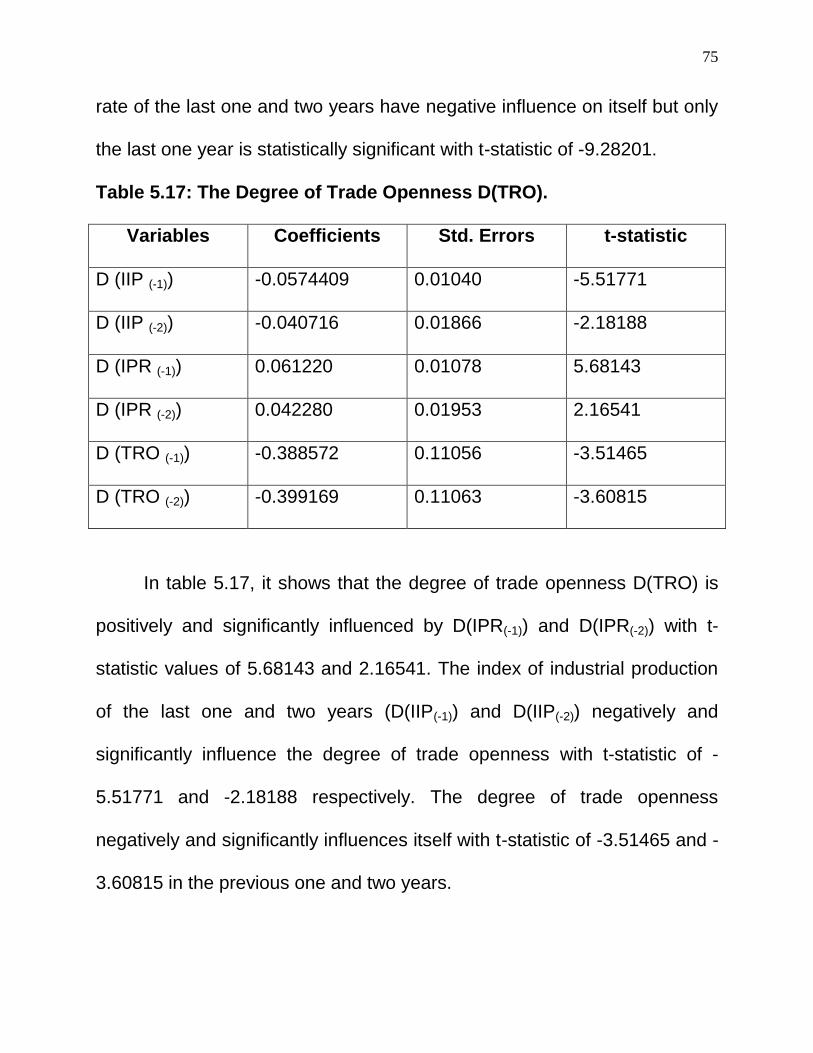
75
rate of the last one and two years have negative influence on itself but only
the last one year is statistically significant with t-statistic of -9.28201.
Table 5.17: The Degree of Trade Openness D(TRO).
Variables Coefficients Std. Errors t-statistic
D (IIP (-1)) -0.0574409 0.01040 -5.51771
D (IIP (-2)) -0.040716 0.01866 -2.18188
D (IPR (-1)) 0.061220 0.01078 5.68143
D (IPR (-2)) 0.042280 0.01953 2.16541
D (TRO (-1)) -0.388572 0.11056 -3.51465
D (TRO (-2)) -0.399169 0.11063 -3.60815
In table 5.17, it shows that the degree of trade openness D(TRO) is
positively and significantly influenced by D(IPR(-1)) and D(IPR(-2)) with t-
statistic values of 5.68143 and 2.16541. The index of industrial production
of the last one and two years (D(IIP(-1)) and D(IIP(-2)) negatively and
significantly influence the degree of trade openness with t-statistic of -
5.51771 and -2.18188 respectively. The degree of trade openness
negatively and significantly influences itself with t-statistic of -3.51465 and -
3.60815 in the previous one and two years.
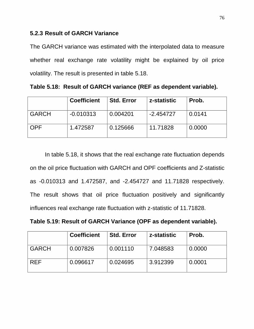
76
5.2.3 Result of GARCH Variance
The GARCH variance was estimated with the interpolated data to measure
whether real exchange rate volatility might be explained by oil price
volatility. The result is presented in table 5.18.
Table 5.18: Result of GARCH variance (REF as dependent variable).
Coefficient Std. Error z-statistic Prob.
GARCH -0.010313 0.004201 -2.454727 0.0141
OPF 1.472587 0.125666 11.71828 0.0000
In table 5.18, it shows that the real exchange rate fluctuation depends
on the oil price fluctuation with GARCH and OPF coefficients and Z-statistic
as -0.010313 and 1.472587, and -2.454727 and 11.71828 respectively.
The result shows that oil price fluctuation positively and significantly
influences real exchange rate fluctuation with z-statistic of 11.71828.
Table 5.19: Result of GARCH Variance (OPF as dependent variable).
Coefficient Std. Error z-statistic Prob.
GARCH 0.007826 0.001110 7.048583 0.0000
REF 0.096617 0.024695 3.912399 0.0001
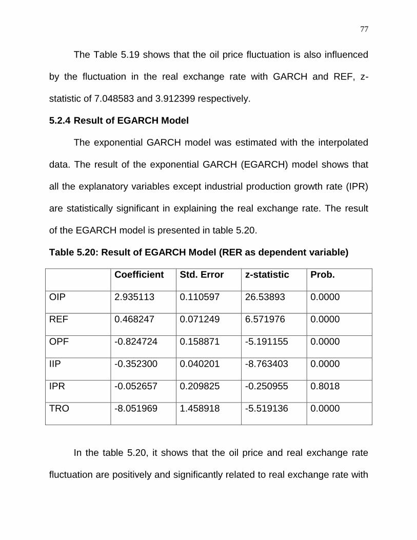
77
The Table 5.19 shows that the oil price fluctuation is also influenced
by the fluctuation in the real exchange rate with GARCH and REF, z-
statistic of 7.048583 and 3.912399 respectively.
5.2.4 Result of EGARCH Model
The exponential GARCH model was estimated with the interpolated
data. The result of the exponential GARCH (EGARCH) model shows that
all the explanatory variables except industrial production growth rate (IPR)
are statistically significant in explaining the real exchange rate. The result
of the EGARCH model is presented in table 5.20.
Table 5.20: Result of EGARCH Model (RER as dependent variable)
Coefficient Std. Error z-statistic Prob.
OIP 2.935113 0.110597 26.53893 0.0000
REF 0.468247 0.071249 6.571976 0.0000
OPF -0.824724 0.158871 -5.191155 0.0000
IIP -0.352300 0.040201 -8.763403 0.0000
IPR -0.052657 0.209825 -0.250955 0.8018
TRO -8.051969 1.458918 -5.519136 0.0000
In the table 5.20, it shows that the oil price and real exchange rate
fluctuation are positively and significantly related to real exchange rate with
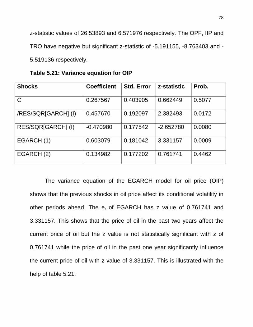
78
z-statistic values of 26.53893 and 6.571976 respectively. The OPF, IIP and
TRO have negative but significant z-statistic of -5.191155, -8.763403 and -
5.519136 respectively.
Table 5.21: Variance equation for OIP
Shocks Coefficient Std. Error z-statistic Prob.
C 0.267567 0.403905 0.662449 0.5077
/RES/SQR[GARCH] (I) 0.457670 0.192097 2.382493 0.0172
RES/SQR[GARCH] (I) -0.470980 0.177542 -2.652780 0.0080
EGARCH (1) 0.603079 0.181042 3.331157 0.0009
EGARCH (2) 0.134982 0.177202 0.761741 0.4462
The variance equation of the EGARCH model for oil price (OIP)
shows that the previous shocks in oil price affect its conditional volatility in
other periods ahead. The et of EGARCH has z value of 0.761741 and
3.331157. This shows that the price of oil in the past two years affect the
current price of oil but the z value is not statistically significant with z of
0.761741 while the price of oil in the past one year significantly influence
the current price of oil with z value of 3.331157. This is illustrated with the
help of table 5.21.
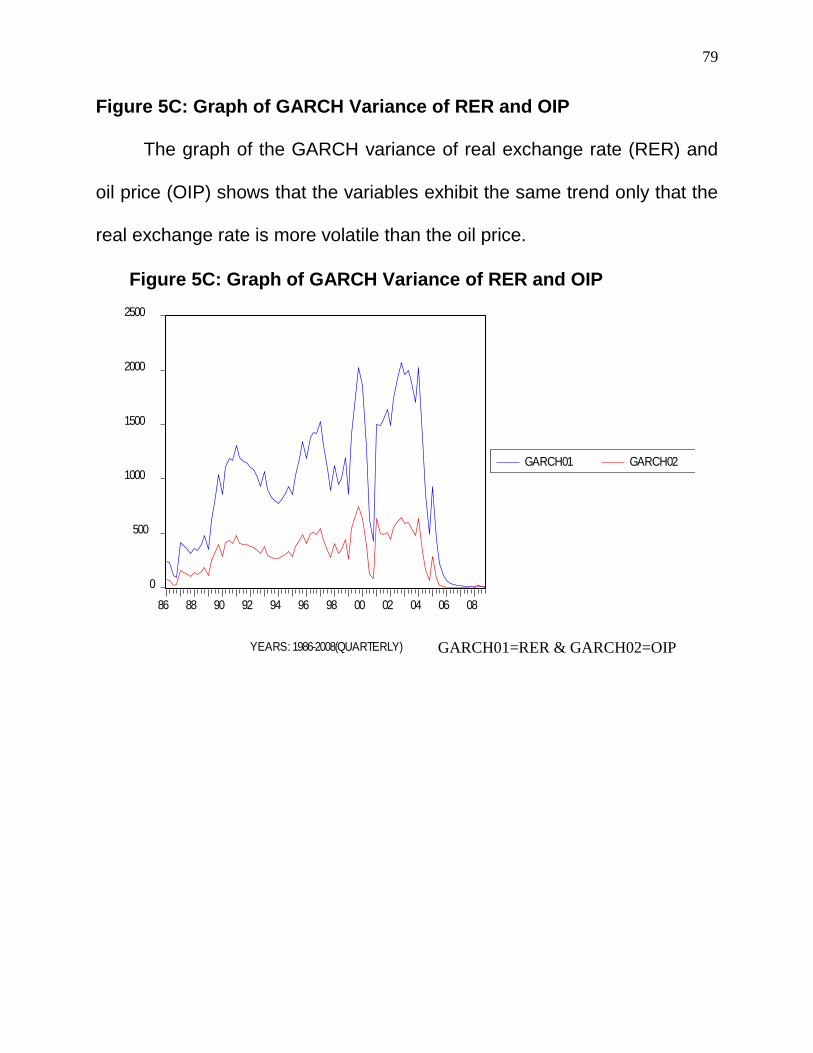
79
Figure 5C: Graph of GARCH Variance of RER and OIP
The graph of the GARCH variance of real exchange rate (RER) and
oil price (OIP) shows that the variables exhibit the same trend only that the
real exchange rate is more volatile than the oil price.
0
500
1000
1500
2000
2500
86 88 90 92 94 96 98 00 02 04 06 08
GARCH01 GARCH02
FIGURE 5J: GRAPH OF GARCH VARIANCE OF RER AND OIP
YEARS: 1986-2008(QUARTERLY) GARCH01=RER & GARCH02=OIP
Figure 5C: Graph of GARCH Variance of RER and OIP
80
5.3.0 EVALUATION OF HYPOTHESES
In this section, we tested the four hypotheses in accordance with the
analysis of the results.
5.3.1 Test of Hypothesis One
Ho: Real exchange rate volatility cannot be explained by oil price volatility in
Nigeria.
Hi: Real, exchange rate volatility can be explained by oil price volatility in
Nigeria.
The result of the GARCH variance shows that the real exchange rate
fluctuation (REF) depends on the oil price fluctuation (OPF) with coefficient
and z-statistic as 1.472587 and 11.71828 respectively. (See table 5.18).
With z-statistic being statistically significant, we therefore, reject the null
hypothesis and accept the alternative hypothesis that says that real
exchange rate volatility can be explained by oil price volatility in Nigeria.
5.3.2 Test of Hypothesis Two
H0: There is no significant impact of oil price shocks on real exchange rate
fluctuations in Nigeria.
Hi: There is significant impact of oil price shocks on real exchange rate
fluctuations in Nigeria.
81
The result of the co-integration test shows that there is impact of oil
price shocks on real exchange rate fluctuations because the two variables
are co-integrated at 5% level of significance (see table 5.5). Equally, results
of the co-integration test of the macro economic variables under study
shows that there are four (4) co-integrating equations. This shows that
there is impact of oil price shocks on real exchange rate fluctuation and on
some other macro-economic variables used in this study. There is close
relationship between these variables. We, therefore, reject the null
hypothesis and accept the alternative that says that; there is significant
impact of oil price shocks on real exchange rate fluctuations in Nigeria.
5.3.3 Test of Hypothesis Three
H0: There is no transmission of shocks from oil price and real exchange
rate fluctuation to some macroeconomic variables in Nigeria.
Hi: There is transmission of shocks from oil price and real exchange rate
fluctuation to some macroeconomic variables in Nigeria.
The result of the parsimonious vector Error correction (VEC) model
(tables 5.11-17) shows that there is transmission of shocks among
variables. The estimated impulse response function indicates significant
transmission of shocks among some of the variables. We, therefore, reject
the null hypothesis and accept the alternative hypothesis that says that;
82
there is transmission of shocks from oil price and real exchange rate to
some macroeconomic variables in Nigeria.
5.3.4 Test of Hypothesis Four
H0: Current shock on oil price has no relationship with its conditional
volatility in periods ahead.
Hi: Current shock on oil price has relationship with its conditional volatility in
periods ahead.
We estimated an asymmetric quadratic function centered at et = 0
with different slopes for positive and negative shocks. This represents
equation 4.18 in chapter four: the result of negative shocks,
NIC (et/ht=2
) = Aexp
11
for et<0, the variance equation shows
0.457670 for et of GARCH and 0.603079 for et of EGARCH. The et of
EGARCH is positively statistically significant and has a z-statistic of
3.331157. The result shows that negative shocks trigger off expectation of
future rise in price thereby creating a positive response. For positive
shocks, the result of
NIC (et/ht = 2 ) = Aexp
1
for et>0, the variance equation shows -
0.470980 for et of GARCH and 0.134982 for et of EGARCH. The result
shows that positive shocks are statistically significant only for et of GARCH
83
with z-statistic of -2.652780 and insignificant for et of EGARCH with
z-statistic of 0.761741.
This shows that positive shocks will create a negative response. We,
therefore, reject the null hypothesis and accept the alternative hypothesis
that says that; current shock on oil price has relationship with its conditional
volatility in periods ahead.

84
CHAPTER SIX
6.0 SUMMARY, POLICY RECOMMENDATION AND CONCLUSION
6.1 Summary
A large literature exists on the theoretical and empirical linkages
between energy and economic growth. Energy, especially oil is a critical
input in many production processes and therefore a causal factor for
economic growth. It is no wonder, therefore, that the demand, supply, and
price of crude oil attract so much attention. This is because Nigeria
depends primarily on oil exportation as her main source of revenue
generation. The economic activities in Nigeria are sensitive to oil price
shock and exchange rate fluctuations. Both local and international oil price
affect industrial activities in Nigeria. The industrial productions in Nigeria
depend mainly on oil to power generating machines for energy supply
because of constant electricity outages. The oil, as the main international
tradable commodity of Nigeria, its price somewhat affect the exchange rate
of naira to other currencies. Also, Nigeria as a net importer of industrial
capital inputs, international oil price fluctuation does affect the real
exchange rate of naira to other currencies.
Between 1975 and 2000, Nigeria‟s broad macroeconomic aggregates
– growth rate, the terms of trade, the real exchange rate, government
85
revenue and spending were among the most volatile in the developing
world. Some macroeconomic variables‟ volatility has become a key
determinant as well as a consequence of poor economic management in
Nigeria. The rate at which different macroeconomic variables are
fluctuating has constituted severe problems for policy analysts. The
exchange rate is arguably the most difficult macroeconomic variable to
model empirically. Surveys of exchange rate models centered on monetary,
purchasing power parity (PPP) models and later on structural time-series
models have been conducted. It has long been recognized that if one could
find a missing real shock that were sufficiently volatile to influence
exchange rate, one could potentially take an important steps towards
resolving the PPP puzzle. This is why the adoption of different exchange
rate regimes to minimize such fluctuations in the Nigerian economy could
not achieve significant results.
Many economic researchers have used cross-country regression
models to find out the causes of fluctuation in exchange rate in many
countries. Many of these researches could not yield significant results
because some of the techniques employed suffer from either inappropriate
measurement or specification bias or both. The results may not also be
86
robust because of the heterogeneity of macroeconomic data, especially
those data from the developing countries.
We adopted a country specific approach to the study. This work
adopted the generalized autoregressive conditional Heteroscedasticity
(GARCH) variance, Exponential Generalized Authoregressive conditional
Heteroscedasticity (EGARCH) and vector Error correction (VEC) models to
capture different hypotheses specified in the work. The result of the
GARCH variance using real exchange rate fluctuation as dependent
variable shows that oil price fluctuation, positively and significantly
influence real exchange rate fluctuation with z-statistic of 11.71828 and
with coefficient of 1.472587. The graph of the GARCH variance of real
exchange rate (RER) and oil price (OIP) shows that the variables exhibit
the same trend only that the real exchange rate is more volatile than the oil
price. Equally, the result of the co-integration test shows that there is
impact of oil price shocks on real exchange rate fluctuations because the
two variables are co-integration at 5% level of significance.
The VEC model result shows that there is transmission of structural
shocks among the variables. The result shows that there is positive
relationship between real exchange rate fluctuation and oil price fluctuation
87
of the last two years with a coefficient of 0.807405 and t-statistic of
1.69163.
The index of industrial production of the last one year negatively and
significantly influences the oil price fluctuation with t-statistic of -2.04052.
We observed from the result that the industrial production growth rate of
the last one and two years negatively and significantly affect the index of
industrial production. Equally, real exchange rate fluctuation is positively
influenced by industrial production growth rate of the last one and two
years. The D(IIP(-1)) and (-2); D(IPR(-1)) and (-2), D(TRO(1) and (-2)) have
significant influence on degree of trade openness. The degree of trade
openness negatively influences itself while industrial production growth rate
has positive and significant influence on trade openness. The index of
industrial production exacts a negative and significant influence on the
degree of trade openness. The real exchange rate (RER) is significantly
influenced by index of industrial production of the previous year with z-
statistic of 4.83197. The oil price is positively and significantly influenced by
index of industrial production of the previous one year with z-statistic of
9.08768.
The result of the exponential GARCH (EGARCH) model shows that
all the explanatory variables except industrial production growth rate (IPR)
88
are statistically significant in explaining the real exchange rate. The real
exchange rate is positively and significantly related to oil price with z-
statistic of 26.53893. The result equally shows that oil price fluctuation,
index of industrial production, and degree of trade openness are negatively
and significantly related to real exchange rate. The variance equation of the
EGARCH model for oil price (OIP) shows that the previous shocks in oil
price affect its conditional volatility in other periods. The et of EGARCH has
z-values of 3.331157 and 0.761741 showing that the shocks in oil price for
the past two years is not significantly related to the price of oil in the current
year but the past one year price of oil significantly determine the price of
the current year with z-value of 3.331157.
6.2 Policy Implications
The results of the research show that the real exchange rate is very
much affected by the fluctuations in international oil price, index of
industrial production, industrial production growth rate, international oil
price, real exchange rate fluctuation, and degree of trade openness. The
variance of oil price and real exchange rate exhibit the same trend but real
exchange rate is more volatile than the oil price. This shows that any little
change in oil price produces a greater change in real exchange rate. That
is, a unit increase or decrease in oil price produces more than a unit
89
increase or decrease in real exchange rate. There is need to ensure
persistent and positive increase in international oil price. Any trade policy
towards this direction will enhance the real exchange rate in Nigeria.
The result equally indicates that international oil price fluctuations,
index of industrial production, and industrial production growth rate are
negatively and significantly related to real exchange rate. This goes to
show that frequent and unpredictable change in oil price produces a
decrease in real exchange rate. This calls for a stable positive increase in
the international oil price. The industrial production growth rate is negatively
related to real exchange rate because most of our industries are heavily
dependent on imported inputs for their industrial production. For this
reason, there is heavy import demand for industrial inputs more than
exports, and this places pressure on foreign exchange demand. There is
need to encourage export oriented industries that use local inputs for the
production of their goods. There should equally, be government, concerted
efforts towards boosting the agricultural production. Policies to encourage
these sectors and strategies toward effective implementation of already
existing ones should be put in place. The small and medium scale
Enterprises (SMEs) that use local inputs should be encouraged. Export
promotion industries should be the target policy of the government. There

90
should be a shift of attention away from the oil and service sectors as the
major sources of government revenue to the real sectors agricultural and
industrial sectors that can produce import substitution goods with greater
local inputs.
Our findings equally reveal that degree of trade openness has
negative relationship with the index of industrial production. This goes to
show that exposure of our industries to outside competition produces a
negative result. To encourage our industries to grow, demands that there
should be some protections from outside competition.
Therefore, the federal government policies on deregulation and trade
liberalization should be embraced with caution because of the negative
effect that over-liberalization will cause on the industrial growth and real
exchange rate in Nigeria.
Application of outcomes of intensive researches and technical
education can help to alleviate the economy from over dependency on oil
and its frequent price shocks. This study for its expository approach to the
causes of real exchange rate fluctuation, structural transmission among the
variables and current shocks on the real exchange rate are useful guideline
for forecasting and policy adjustment.

91
6.3 Recommendations
The exchange rate fluctuation is demand propelled. To stabilize the
naira exchange rate, we recommend increased non-oil export receipts. The
exchange rate volatility cannot be stable through exchange rate
management alone but could be achieved through increased non-oil export
receipts, especially of the basket of currencies – US dollar, British pound
sterling, German Deutschemark, Swiss Francs, French Francs, Japanese
Yen and Dutch guilder. The government external sector policy should focus
on policies that will ensure foreign exchange earnings so that demand
pressure on foreign exchange will be matched with supply. The increase in
foreign exchange earnings through increase in non-oil export will ensure
increased foreign exchange reserves; improve the credit worthiness and
competitiveness of the economy. It will equally strengthen the naira and
move the naira towards equal convertibility to US dollar.
We equally note, that Nigerian oil sector has a lot of contradictions
that play a major role in naira exchange rate. The contradiction is more
glaring with rise in crude oil prices at the global markets, the rise will mean
more external earnings for Nigeria but will increase the expense burden on
imported refined petroleum products. To remove this obvious contradiction,
we recommend that our local refineries should be resuscitated to full
92
operation and capacity. We equally, note that the retained foreign
exchange earnings from the crude oil sales by the oil companies bring
imbalance between demand and supply of foreign exchange. We
recommend that the government should enter into negotiation with the oil
companies to reduce their retaining capacity of foreign exchange and
encourage them to reinvest it in the country. This could be done through
certain encouraging concessions to such reinvestments.
6.4 Conclusion
The unstable and unpredictable nature of the oil price process makes
it a textbook example of the non-discrete jump process. Many policy
analysts have come to conclude that there is multiple equilibrium
explanation for oil price. On the other hand, a good number of researchers
studying exchange rate prediction have concluded that the best single
predictor of the exchange rate next period – tomorrow, next week, next
month, maybe even next year – is the exchange rate this period.
Obviously, many of these researches failed to capture the causes of
real exchange rate fluctuation and to predict the real exchange rate,
because of the monetary model approach and purchasing power parity
models used that made so many unrealistic assumptions. The cross-
country regression approach adopted by later researchers focused on oil

93
importing countries as well as cross-country data for the regression
analysis. Many of these researches could not yield significant results
because some of the techniques employed suffer from either inappropriate
measurement or specification bias or both. The results were not robust
because of the heterogeneity of macroeconomic data, especially those
data from the developing countries.
This study found out that real exchange rate fluctuation in Nigeria is
significantly influenced by oil price shocks, index of industrial production,
real exchange rate fluctuation, international oil price and industrial
production growth rate. Any policy to address the issue of real exchange
rate volatility in Nigeria should give priority to oil price changes, and the rest
of the variables. There are transmission of shocks among real exchange
rate and the rest of the variables. The rates of transmission of shocks
among these variables are useful for policy adjustment. The graph of the
GARCH variance of real exchange rate and oil price shows that the
variables exhibit the same trend only that the real exchange rate is more
volatile than the oil price. This shows that any little change in oil price
produces a greater change in real exchange rate. That is to say a unit
increase or decrease in oil price produces more than a unit increase or
decrease in real exchange rate. There is need to ensure persistent and
94
positive increase in international oil price. Any trade policy towards this
direction will enhance the real exchange rate in Nigeria. This study equally,
reveals that degree of trade openness has negative relationship with the
index of industrial production. This implies that exposure of our industries
to outside competition produces a negative result. There is need to focus
research attention on acceptable degree of trade openness to avoid over-
liberalization of the economy. There is also need for more researches on
this area of our study using different approaches and/or variables for more
exposition of the area.
95
REFERENCES
Agu, C. (2002), “Real Exchange Rate Distortions and External Balance Position of Nigeria: Issues and policy options”. Journal of African Finance and Economics; Department; Institute of African American Affairs, New York University.
Amano, R and Van Norden S. (1998), “Oil Prices and the rise and fall of the U.S. real exchange rate”. Journal of International Money and Finance, 17 p. 299 – 316.
Amano, R. and Van Norden, S. (1995), “Terms of Trade and Real Exchange rates: The Canadian Evidence”. Journal of International Money and Finance, 14, p. 83 – 104.
Amin, A.A. and Awung, W.J. (1997): “Determinants of Real Exchange Rates in Cameroon”, African Journal of Economic Policy Vol. 4 Number 1.
Asea, P. and E. Mendoza, (1994); The Balassa-Samuelson Model: A General-Equilibrium Appraisal. Review of International Economics, 2, 244-67
Backus, D. and Crucini, M. (1998), “Oil prices and the Terms of Trade”. NBER Working Paper No. 6697
Baffes, John, Elbadawi, Ibrahim, and O‟Connel, Stephen (1997), “Single Equation Estimation of the Equilibrium Real Exchange Rate” Policy Research Working Paper, Washington D.C; The World Bank.
Baffes, John, Elbadawi, Ibrahim, and O‟Connel, Stephen (1999). “Single Equation Estimation of the Equilibrium Real Exchange Rate” In Hinkle, L.E. and Montiel, P.J. (eds) Exchange Rate Misalignment: Concepts and Measurement for Developing Countries. Pp. 405 – 465 The World Bank: Oxford University Press.
Baxter, Marianne (1994), “Real Ex change Rates, Real Interest Differentials, and Government Policy: Theory and Evidence” Journal of Monetary Economics 33: 5 – 37.
96
Blanchard, Oliver J. and Danny Quah (1989), “The Dynamic Effect of Aggregate Demand and Supply Distrubance”. American Economic Review 79: 655 – 73
Blundell-Wignall, Adrian and Frank Browne, (1991), “Increasing Financial Market Integration Real Exchange Rates and Macroeconomic Adjustment” OECD Working Paper 96 Feb.
Bollerslev, T. (1986): “Generalized Auto-Regressive Conditional Heteroscedasticity”. Journal of Econometrics. 307-27
Buiter, Willen (1999), “The Emu and the NAMU: What is the Case for North American Monetary Union?” Canadian Public Policy 25, 285 – 305.
Campbell, John Y and Rihard H. Clarida (1987), “The dollar and real interest rates”, Carnegie – Rochester Conference Series on Public Policy 27: 103 – 40.
Carruth, A.A., M.A.Hooker and A.J. Oswald (1996), “Unemployment Equilibria and Input Prices: Theory and Evidence for the United States”, Review of Economics and Statistics.
Cashin, P.; H. Liang and C.J. Mcdermoth (2000), “How Persistent are Shocks to World Commodity Prices? IMF Staff Papers, Vol. 47 (2).
CBN (2000), “The Changing Structure of the Nigerian Economy and Implications for Development”. Published by Realm Communications Ltd. Lagos
Chen, Y. and Rogoff, K. (2001), “Commodity Currencies and Empirical Exchange Rate Equations”. Unpublished Paper Prepared for Empirical Exchange Rate Models Conference in Madison Wisconsin.
Cheung, Yin-Wong: Menzie, D. Chinn; and Antonio Garcia Pascual, (2002), “Empirical Exchange Rate Models of the Nineties: Are Any Fit to Survive?” Mimeo, Department of Economics. University of California B. Santa Cruz.
97
Clarida, Richard H. and Jordi Gali (1994), “Sources of Real Exchange Rate Fluctuations: How Important are Nominal Shocks?” Working Paper No. 4658. NBER, Cambridge, M.A.
Cooley Thomas .F. and Stephen.F.Leroy,(1985) “Theoretical Macroeconomics: A Critique”. Journal of Monetary Economics, Vol. 16.
Cushman, David O, Sang S. Lee and Thorsteinn Thorgeirsson (1995), “Maximum Likelihood Estimates of Co integration in Exchange Rate Models for Seven Inflationary OECD Countries”. Journal of International Money and Finance.
Daniel, N.C. (1997), “International Interdependence of National Growth Rates: A Structural Tends Analysis”, Journal of Monetary Economics 40: 73 – 96.
David, T.K. (2003), “USAID/Nigeria Economic Growth Activities Assessment: Transition Period Summary Report”. IBM Business Consulting Services 1616 North Fort Myer Drive Arlington, VA 22209.
Davidson, Russel and G.James Mackinnon,(1993): Estimation and Inference in Econometrics. Oxford University Press.
De Gregorio, J. and H. Wolf,. (1994), “Terms of Trade, Productivity and the Real Exchange Rate”. NBER Working Paper No. 4807.
Dibooglu, Selahattin (1995), “Real Disturbances, Relative Prices, and Purchasing Power Parity” Southern Journal of Economics.
Dickey, David A and Wayne A. Fuller (1979), “Distribution of the Estimator of Autoregressive Time Series with a Unit Root”. Journal of the American Statistical Association 74: 427 – 31
Dornbusch, Rudiger (1988): “Exchange Rates and Inflation”. The MIT Press Cambridge, Massachusetts, London, England
Dornbush, R. (1987); Exchange Rates and Prices. American Economic Review 77 (March), 95-106
98
Dotsey, M. and M. Reid (1992), “Oil Shocks, Monetary Policy and Economic Activity”. Economic Review. Federal Reserve Bank of Richmond, Richmond, V.A. 14 – 27.
Edison, Hail J. and B.D. Paul‟s (1993), “A Re-assessment of the Relationship Between Real Exchange Rates and the Real Interest Rates: 1974 – 1990”. Journal of Monetary Economics 31: 165 – 187
Edwards, Sebastian, (1989). Real Exchange Rate Devaluation and Adjustment. Cambridge: MIT.
Elbadawi, Ibrahim A., and Soto, Raimundo (1995b), “Real Exchange Rate and Macroeconomic Adjustment in Sub-Saharan Africa And Other Developing Countries” AERC Plenary Session. Journal of African Economics, Supplement to Vol. 6 No. 3. Nairobi.
Elbadawi, Ibrahim A.; and Soto, Raimundo (1995b). “Real Exchange Rate And Macroeconomic Adjustment in Sub-Saharan Africa And Other Developing Countries” AERC Plenary Session, Journal of African Economics, Supplement to Vol. 6 No.3 Nairobi.
Engel, C. (1999), Accounting for U.S. Real Exchange Rate Changes. Journal of Political Economy, 107, 507 – 537.
Engel, Charles (2002), “Expenditure Switching and Exchange Rate Policy”, National Bureau of Economic Research, Working Paper No # # # #
Engle, R and C.W.J. Granger, (1987); “co-integration and Error Correction: Representation, Examinatin and Testing”. Econometrica Vol. 55 No 2 PP 251-276.
Engle, R.F (1982): “Autoregressive Conditional Heteroscedasticity with Estimates of the Variance of United Kingdom Inflation”. Econometrica 50, 987-1007
Evans, Martin D.D. and James R. Lothian (1993), “The response of exchange rates to permanent and transitory Shock under Floating Exchange Rates”. Journal of International Money and Finance
99
Farrell, G.N.; B. Kahn and F.J. Visser,(2001), “Price Determination in International Oil Markets: Developments and Prospects”. SARB Quarterly Bulletin No. 219, March 2001, 69 – 88.
Friedman, Milton (1953), “The case for Flexible Exchange Rates”, in Essays in Positive Economics (Chicago: University of Chicago Press), 157 – 203.
Friedman, Milton (1953), “The Case for Flexible Exchange Rates”, in Essays in Positive Economics, University of Chicago Press, Chicago, 157 – 203.
Froot, Kenneth A. and Kenneth Rogoff (1994), “Perspectives on PPP and Long-Run Real Exchange Rates”. NBER Working Paper. No. 4952 The Handbook of International Economics.
Gardeazabal, Javier and Marta Regulez (1992), “The Monetary Model of Exchange rates and Cointegration: Estimation, Testing and Prediction. Springer – Verlag.
Gbadebo, O.O (2007), “Crude Oil and the Nigerian Economic Performance” Oil and Gas Business. http.//www.Ogbus.ru/eng/
Godbout, Marie-Josee and Simon Van Norden (1995), “Reconsidering Cointegration in Exchange rates: Case studies of size distortion in finite Samples”. Manuscript for presentation at the 1996 Winter Meetings of the Econometric Society.
Gonzalo, Jesus and J. Y. Pitarakis (1994), “Cointegration Analysis in Large Systems”. Mimeo. Boston University, Boston, M.A.
Hamilton, J. D. (1996), “This is what Happened to the Oil- Price Macroeconomy Relationship”, Journal of Monetary Economics 38: 215 – 20.
Hamilton, James D. (1983), “Oil and the Macroeconomy Since World War II”. Journal of Political Economy 91: 228 – 48.
Hamilton, James D. (1994): Time Series Analysis. Princeton University Press.
Hooker, M.A. (1996), “What Happened to the oil price Macroeconomy Relationship?” Journal of Monetary Economics 38: 195 – 312.
100
Hooper, Peter and Catherinel Mann, (1989). “The Emergence And Persistence of the U.S. External Imbalance 1980 – 1987.” Princeton Studies in International Finance. New Jersey No. 65 October, Princeton University.
Huizinga J. (1987), “An Empirical Investigation of the Long-run Behaviour of Real Exchange Rates”. Carnegie – Rochester Series on Public Policy, 27, 149 – 215.
International Energy Agency (IEA)(2005), “Energy Balances of OECD countries and Energy Balances of Non-OECD Countries (2003 Edition)”, Paris: IEA.
JEL (1996); “Exchange Rates and Oil Prices” JEL Classification Codes: F 31.
Jimenez – Rodigruez, R; and M. Sanchez (2003), “Oil Price Shocks and Real GDP Growth: Empirical Evidence from Some OECD countries” Mimeo
Johansen, Seroen and Katarina Juselius (1990) “The full Information Maximum Likelihood Procefure for Inference on Cointegration”. Oxford Bulletin of Economics and Statistic 52: 169 – 210.
Kenneth D. West, (2003), “Monetary Policy and the Volatility of Real Exchange Rates in New Zealand”. University of Wisconsin. JEL Classification: E52, F31, C51 Discussion Paper Series. Reserve Bank of New Zealand.
Kim, I.M and P. Loungani (1992), “The Role of Energy in Real Business Cycles”. Journal of Monetary Economics, 29: 173 – 189.
Komolafe, Oluranti Stella (1995), “Exchange Rate Management in Small Open Developing Economies: Some Theoretical Considerations” External Trade and Economic Development in Nigeria. Selected Paper for the Annual Conference of Nigeria Economic Society Ibadan.
Krugman, (2000); Energy Crisis Revisited. Available at www.mit.edu/krugman.
101
Krugman, P. (1983), “Oil and the Dollar”. In: Bhandari, J. and Putman, B. (Eds): Economic Interdependence and Flexible exchange rates. MIT Press; Cambridge, M.A.
Lahtinen, M, (2000); Long-Run Deviations from the Purchasing Power Party Between German Mark and US Dollar-Oil Price, the Missing Link? Unpublished Mimeo, University of Tampere.
Lahtinen, M. (2001), “The U.S. Dollar Real Exchange rate and oil price: A real Option approach”. A draft Department of Economics, University of Tampere.
Lahtinen, M. (2002), “Long-run Deviations from the Purchasing Power Parity between German Mark and U.S. Dollar – oil price, the missing link?” Unpublished Mimeo, University of Tampere.
Lastrapes, William D. (1992), “Sources of Fluctuations in Real and Normal Exchange Rates”. Review of Economics and Statistics 74: 530 – 39
Loungani, P. (1986), “Oil Price Shocks and the Dispersion Hypothesis”. Review of Economics and Statistics 68: 536 – 39.
MacDonald, Ronald and Mark P. Taylor (1994), “The Monetary Model of the Exchange Rate: Long-Run Relationships, Short-Run Dynamics and How to Beat a Random Walk”. Journal of International Money and Finance 13: 276 – 90.
McGuirk, Anne K. (1983), “Oil Price Changes and Real Exchange Rate Movements among Industrial Countries”, International Monetary Fund Staff Papers 30: 843 – 83.
Meese, R.A. (1990); “Currency Fluctuations in the Post-Bretton Woods Era”. Journal of Economic Perspectives 4. 117-34.
Meese, Richard A. and Kenneth Rogoff (1983), “Empirical Exchange Rate Models of the Seventies: Do they fit out of sample?” Journal of International Economics 14: 3 – 24.
Meese, Richard A. and Kenneth Rogoff (1988), “Was it real: The Exchange Rate-Interest Differential Relation Over the Modern Floating – Rate Period”. The Journal of Finance 43: 933 – 48.
102
Montiel, Peter J, (1999); “Determinants of Long Run Equilibrium Real Exchange Rate” in Hinkle, L.E and P.T. Montiel, (eds) Exchange Rate Misalignment: Concepts and Measurement for Developing Countries. Pp 264-289 The World Bank: Oxford University Press.
Mork, K.A. (1994), “Business Cycles and the Oil Market”, Energy Journal 15, Special Issue pp. 15 – 38.
Mussa, M.L. (1990), “Exchange Rates in Theory and in Reality”. Essays in International Finance, No. 179, Princeton University Department of Economics, International Finance Section, Princeton, N J.
NEEDS (2005), National Planning Commission, Federal Secretariat, Abuja, Nigeria.
Nkomo, J.C, (2006), “The Impact of Higher Oil Prices on Southern African Countries”. Journal of Energy Research in South Africa. 17(1), 10 – 17.
Obstfeld, Maurice and Kenneth Rogoff (1998), “Risk and Exchange Rate”. National Bureau of Economics Research Working Paper, No. 6694.
Obstfeld, Maurice and Kenneth Rogoff (2000a), “New Directions for Stochastic Open Economy Models”, Journal of International Economics 50, 117 – 153.
Obstfeld, Maurice and Kenneth Rogoff. (1995), “Exchange Rate Dynamics Redux”, Journal of Political Economy 103, 624 – 660
Olomola, P.A. and A.V. Adejume,(2006), Oil Price Shock and Macroeconomic Activities in Nigeria. International Research Journal of Finance and Economics ISSN 1450 – 2887 Issue 3 (2006).
Parikh, Ashok (1997) „Determinants of Real Exchange Rates in South Africa: A Short-run and Long-run Analysis‟; African Journal of Economic Policy Vol. 4 No. 1
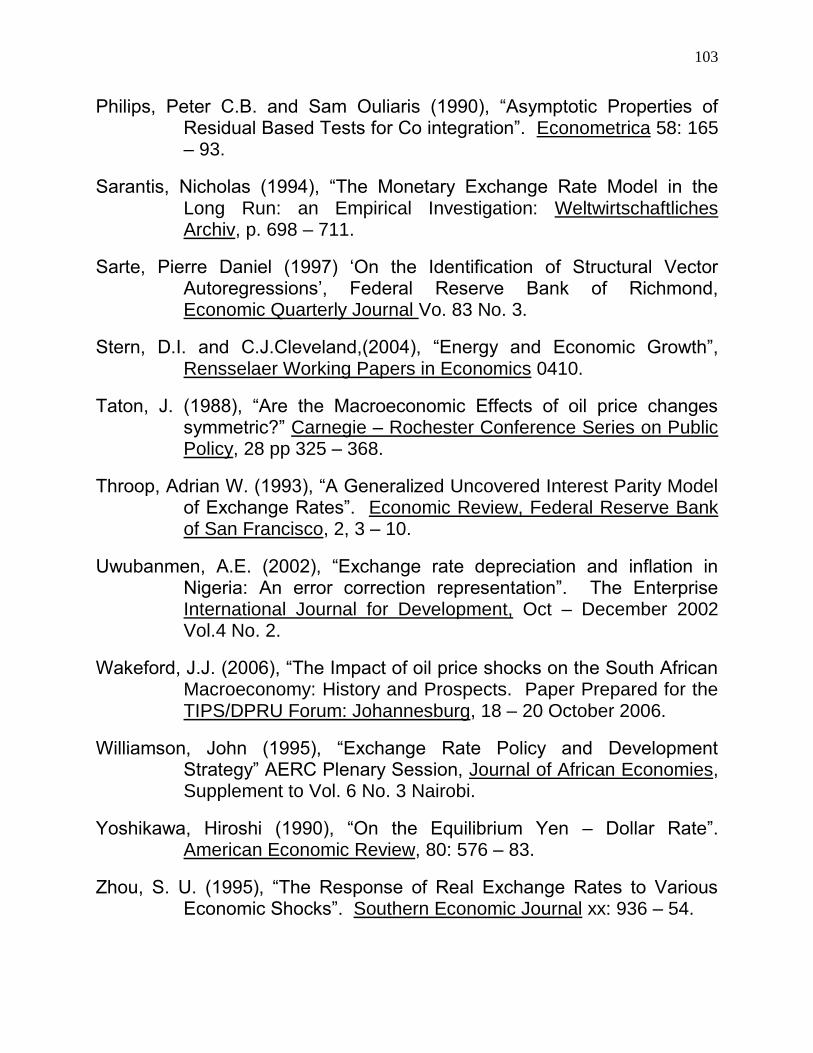
103
Philips, Peter C.B. and Sam Ouliaris (1990), “Asymptotic Properties of Residual Based Tests for Co integration”. Econometrica 58: 165 – 93.
Sarantis, Nicholas (1994), “The Monetary Exchange Rate Model in the Long Run: an Empirical Investigation: Weltwirtschaftliches Archiv, p. 698 – 711.
Sarte, Pierre Daniel (1997) „On the Identification of Structural Vector Autoregressions‟, Federal Reserve Bank of Richmond, Economic Quarterly Journal Vo. 83 No. 3.
Stern, D.I. and C.J.Cleveland,(2004), “Energy and Economic Growth”, Rensselaer Working Papers in Economics 0410.
Taton, J. (1988), “Are the Macroeconomic Effects of oil price changes symmetric?” Carnegie – Rochester Conference Series on Public Policy, 28 pp 325 – 368.
Throop, Adrian W. (1993), “A Generalized Uncovered Interest Parity Model of Exchange Rates”. Economic Review, Federal Reserve Bank of San Francisco, 2, 3 – 10.
Uwubanmen, A.E. (2002), “Exchange rate depreciation and inflation in Nigeria: An error correction representation”. The Enterprise International Journal for Development, Oct – December 2002 Vol.4 No. 2.
Wakeford, J.J. (2006), “The Impact of oil price shocks on the South African Macroeconomy: History and Prospects. Paper Prepared for the TIPS/DPRU Forum: Johannesburg, 18 – 20 October 2006.
Williamson, John (1995), “Exchange Rate Policy and Development Strategy” AERC Plenary Session, Journal of African Economies, Supplement to Vol. 6 No. 3 Nairobi.
Yoshikawa, Hiroshi (1990), “On the Equilibrium Yen – Dollar Rate”. American Economic Review, 80: 576 – 83.
Zhou, S. U. (1995), “The Response of Real Exchange Rates to Various Economic Shocks”. Southern Economic Journal xx: 936 – 54.
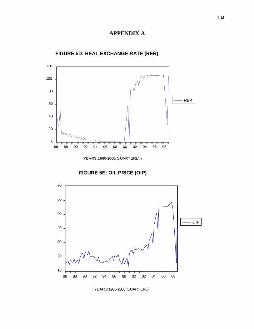
104
APPENDIX A
0
20
40
60
80
100
120
86 88 90 92 94 96 98 00 02 04 06 08
RER
FIGURE 5A: REAL EXCHANGE RATE(RER)
YEARS:1986-2008(QUARTERLY)
10
20
30
40
50
60
70
86 88 90 92 94 96 98 00 02 04 06 08
OIP
FIGURE 5B: OIL PRICE(OIP)
YEARS:1986-2008(QUARTERL)
FIGURE 5D: REAL EXCHANGE RATE (RER)
FIGURE 5E: OIL PRICE (OIP)
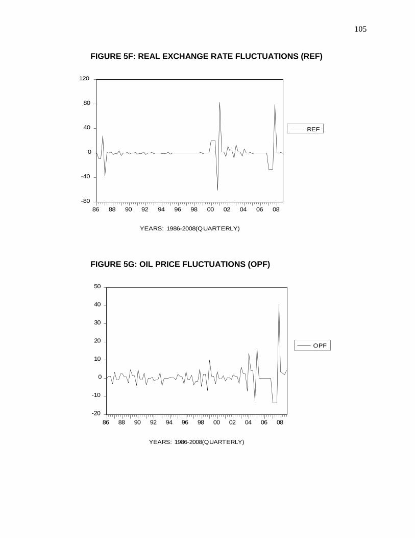
105
-80
-40
0
40
80
120
86 88 90 92 94 96 98 00 02 04 06 08
REF
FIGURE 5C: REAL EXCHANGE RATE FLUCTUATIONS(REF)
YEARS: 1986-2008(QUARTERLY)
-20
-10
0
10
20
30
40
50
86 88 90 92 94 96 98 00 02 04 06 08
OPF
FIGURE 5D: OIL PRICE FLUCTUATIONS(OPF)
YEARS: 1986-2008(QUARTERLY)
FIGURE 5F: REAL EXCHANGE RATE FLUCTUATIONS (REF)
FIGURE 5G: OIL PRICE FLUCTUATIONS (OPF)
106
20
40
60
80
100
120
140
160
86 88 90 92 94 96 98 00 02 04 06 08
IIP
FIGURE 5E: INDEX OF INDUSTRIAL PRODUCTION(IIP)
YEARS: 1986-2008(QUARTERLY)
0
10
20
30
40
50
60
86 88 90 92 94 96 98 00 02 04 06 08
IPR
FIGURE 5F: INDUSTRIAL PRODUCTION GROWTH RATE(IPR)
YEARS: 1986-2008(QUARTERLY)
FIGURE 5H: INDEX OR INDUSTRIAL PRODUCTION (IIP)
FIGURE 5I: INDUSTRIAL PRODUCTION GROWTH RATE (IPR)
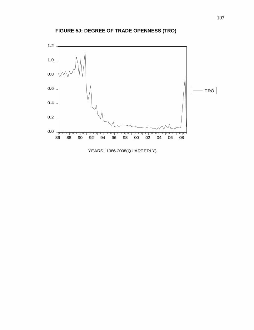
107
0.0
0.2
0.4
0.6
0.8
1.0
1.2
86 88 90 92 94 96 98 00 02 04 06 08
TRO
FIGURE 5G: DEGREE OF TRADE OPENNESS(TRO)
YEARS: 1986-2008(QUARTERLY)
FIGURE 5J: DEGREE OF TRADE OPENNESS (TRO)
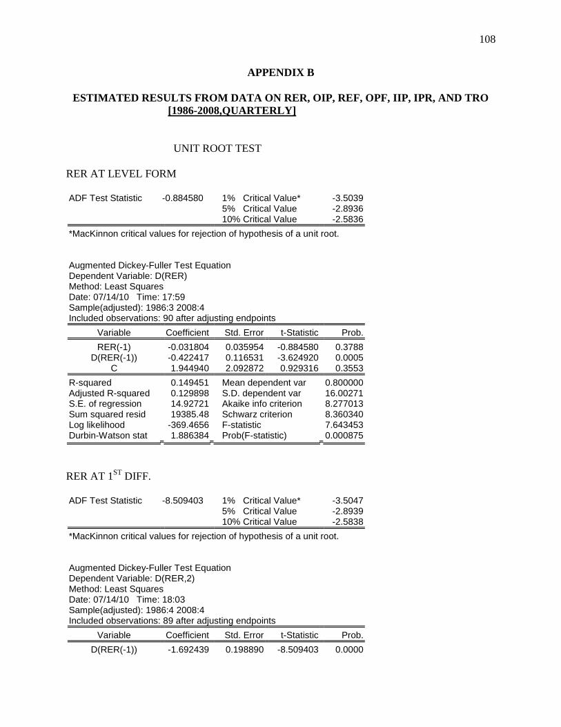
108
APPENDIX B
ESTIMATED RESULTS FROM DATA ON RER, OIP, REF, OPF, IIP, IPR, AND TRO
[1986-2008,QUARTERLY]
UNIT ROOT TEST
RER AT LEVEL FORM
ADF Test Statistic -0.884580 1% Critical Value* -3.5039
5% Critical Value -2.8936 10% Critical Value -2.5836
*MacKinnon critical values for rejection of hypothesis of a unit root.
Augmented Dickey-Fuller Test Equation Dependent Variable: D(RER) Method: Least Squares Date: 07/14/10 Time: 17:59 Sample(adjusted): 1986:3 2008:4 Included observations: 90 after adjusting endpoints
Variable Coefficient Std. Error t-Statistic Prob.
RER(-1) -0.031804 0.035954 -0.884580 0.3788 D(RER(-1)) -0.422417 0.116531 -3.624920 0.0005
C 1.944940 2.092872 0.929316 0.3553
R-squared 0.149451 Mean dependent var 0.800000 Adjusted R-squared 0.129898 S.D. dependent var 16.00271 S.E. of regression 14.92721 Akaike info criterion 8.277013 Sum squared resid 19385.48 Schwarz criterion 8.360340 Log likelihood -369.4656 F-statistic 7.643453 Durbin-Watson stat 1.886384 Prob(F-statistic) 0.000875
RER AT 1ST
DIFF.
ADF Test Statistic -8.509403 1% Critical Value* -3.5047
5% Critical Value -2.8939 10% Critical Value -2.5838
*MacKinnon critical values for rejection of hypothesis of a unit root.
Augmented Dickey-Fuller Test Equation Dependent Variable: D(RER,2) Method: Least Squares Date: 07/14/10 Time: 18:03 Sample(adjusted): 1986:4 2008:4 Included observations: 89 after adjusting endpoints
Variable Coefficient Std. Error t-Statistic Prob.
D(RER(-1)) -1.692439 0.198890 -8.509403 0.0000
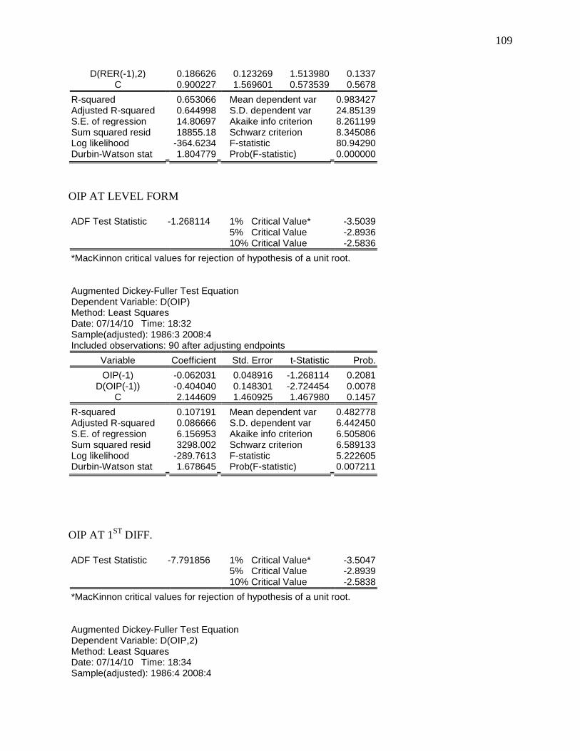
109
D(RER(-1),2) 0.186626 0.123269 1.513980 0.1337 C 0.900227 1.569601 0.573539 0.5678
R-squared 0.653066 Mean dependent var 0.983427 Adjusted R-squared 0.644998 S.D. dependent var 24.85139 S.E. of regression 14.80697 Akaike info criterion 8.261199 Sum squared resid 18855.18 Schwarz criterion 8.345086 Log likelihood -364.6234 F-statistic 80.94290 Durbin-Watson stat 1.804779 Prob(F-statistic) 0.000000
OIP AT LEVEL FORM
ADF Test Statistic -1.268114 1% Critical Value* -3.5039
5% Critical Value -2.8936 10% Critical Value -2.5836
*MacKinnon critical values for rejection of hypothesis of a unit root.
Augmented Dickey-Fuller Test Equation Dependent Variable: D(OIP) Method: Least Squares Date: 07/14/10 Time: 18:32 Sample(adjusted): 1986:3 2008:4 Included observations: 90 after adjusting endpoints
Variable Coefficient Std. Error t-Statistic Prob.
OIP(-1) -0.062031 0.048916 -1.268114 0.2081 D(OIP(-1)) -0.404040 0.148301 -2.724454 0.0078
C 2.144609 1.460925 1.467980 0.1457
R-squared 0.107191 Mean dependent var 0.482778 Adjusted R-squared 0.086666 S.D. dependent var 6.442450 S.E. of regression 6.156953 Akaike info criterion 6.505806 Sum squared resid 3298.002 Schwarz criterion 6.589133 Log likelihood -289.7613 F-statistic 5.222605 Durbin-Watson stat 1.678645 Prob(F-statistic) 0.007211
OIP AT 1ST
DIFF.
ADF Test Statistic -7.791856 1% Critical Value* -3.5047
5% Critical Value -2.8939 10% Critical Value -2.5838
*MacKinnon critical values for rejection of hypothesis of a unit root.
Augmented Dickey-Fuller Test Equation Dependent Variable: D(OIP,2) Method: Least Squares Date: 07/14/10 Time: 18:34 Sample(adjusted): 1986:4 2008:4
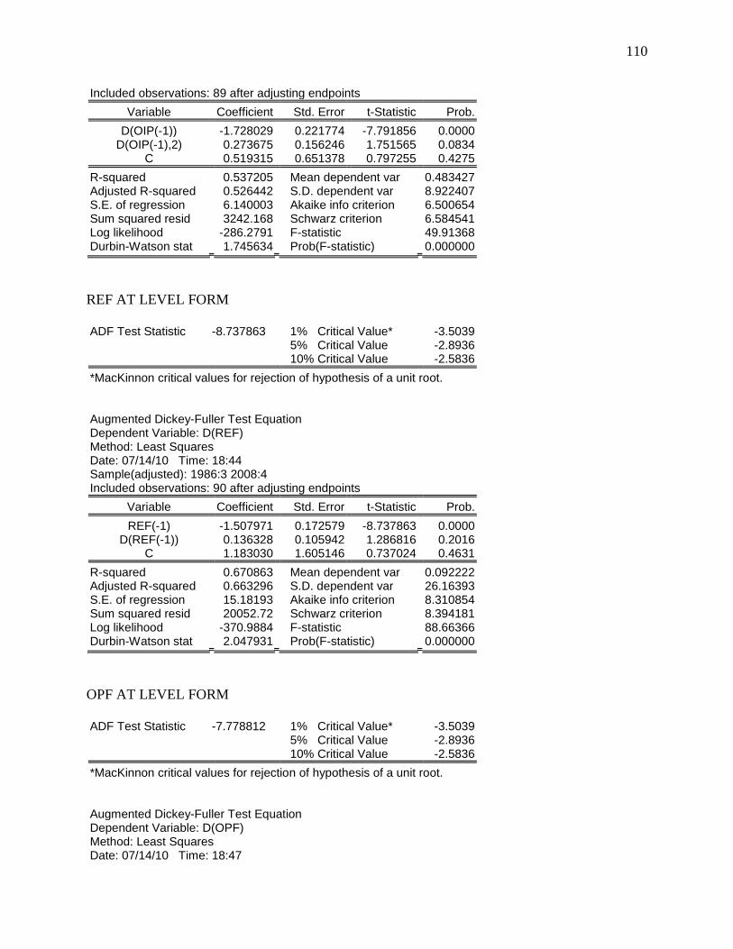
110
Included observations: 89 after adjusting endpoints
Variable Coefficient Std. Error t-Statistic Prob.
D(OIP(-1)) -1.728029 0.221774 -7.791856 0.0000 D(OIP(-1),2) 0.273675 0.156246 1.751565 0.0834
C 0.519315 0.651378 0.797255 0.4275
R-squared 0.537205 Mean dependent var 0.483427 Adjusted R-squared 0.526442 S.D. dependent var 8.922407 S.E. of regression 6.140003 Akaike info criterion 6.500654 Sum squared resid 3242.168 Schwarz criterion 6.584541 Log likelihood -286.2791 F-statistic 49.91368 Durbin-Watson stat 1.745634 Prob(F-statistic) 0.000000
REF AT LEVEL FORM
ADF Test Statistic -8.737863 1% Critical Value* -3.5039
5% Critical Value -2.8936 10% Critical Value -2.5836
*MacKinnon critical values for rejection of hypothesis of a unit root.
Augmented Dickey-Fuller Test Equation Dependent Variable: D(REF) Method: Least Squares Date: 07/14/10 Time: 18:44 Sample(adjusted): 1986:3 2008:4 Included observations: 90 after adjusting endpoints
Variable Coefficient Std. Error t-Statistic Prob.
REF(-1) -1.507971 0.172579 -8.737863 0.0000 D(REF(-1)) 0.136328 0.105942 1.286816 0.2016
C 1.183030 1.605146 0.737024 0.4631
R-squared 0.670863 Mean dependent var 0.092222 Adjusted R-squared 0.663296 S.D. dependent var 26.16393 S.E. of regression 15.18193 Akaike info criterion 8.310854 Sum squared resid 20052.72 Schwarz criterion 8.394181 Log likelihood -370.9884 F-statistic 88.66366 Durbin-Watson stat 2.047931 Prob(F-statistic) 0.000000
OPF AT LEVEL FORM
ADF Test Statistic -7.778812 1% Critical Value* -3.5039
5% Critical Value -2.8936 10% Critical Value -2.5836
*MacKinnon critical values for rejection of hypothesis of a unit root.
Augmented Dickey-Fuller Test Equation Dependent Variable: D(OPF) Method: Least Squares Date: 07/14/10 Time: 18:47
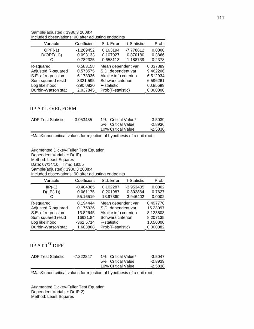
111
Sample(adjusted): 1986:3 2008:4 Included observations: 90 after adjusting endpoints
Variable Coefficient Std. Error t-Statistic Prob.
OPF(-1) -1.269452 0.163194 -7.778812 0.0000 D(OPF(-1)) 0.093133 0.107027 0.870180 0.3866
C 0.782325 0.658113 1.188739 0.2378
R-squared 0.583158 Mean dependent var 0.037389 Adjusted R-squared 0.573575 S.D. dependent var 9.462206 S.E. of regression 6.178936 Akaike info criterion 6.512934 Sum squared resid 3321.595 Schwarz criterion 6.596261 Log likelihood -290.0820 F-statistic 60.85599 Durbin-Watson stat 2.037845 Prob(F-statistic) 0.000000
IIP AT LEVEL FORM
ADF Test Statistic -3.953435 1% Critical Value* -3.5039
5% Critical Value -2.8936 10% Critical Value -2.5836
*MacKinnon critical values for rejection of hypothesis of a unit root.
Augmented Dickey-Fuller Test Equation Dependent Variable: D(IIP) Method: Least Squares Date: 07/14/10 Time: 18:55 Sample(adjusted): 1986:3 2008:4 Included observations: 90 after adjusting endpoints
Variable Coefficient Std. Error t-Statistic Prob.
IIP(-1) -0.404385 0.102287 -3.953435 0.0002 D(IIP(-1)) 0.061175 0.201987 0.302864 0.7627
C 55.16519 13.97860 3.946402 0.0002
R-squared 0.194444 Mean dependent var 0.497778 Adjusted R-squared 0.175926 S.D. dependent var 15.23097 S.E. of regression 13.82645 Akaike info criterion 8.123808 Sum squared resid 16631.84 Schwarz criterion 8.207135 Log likelihood -362.5714 F-statistic 10.50000 Durbin-Watson stat 1.603808 Prob(F-statistic) 0.000082
IIP AT 1ST
DIFF.
ADF Test Statistic -7.322847 1% Critical Value* -3.5047
5% Critical Value -2.8939 10% Critical Value -2.5838
*MacKinnon critical values for rejection of hypothesis of a unit root.
Augmented Dickey-Fuller Test Equation Dependent Variable: D(IIP,2) Method: Least Squares
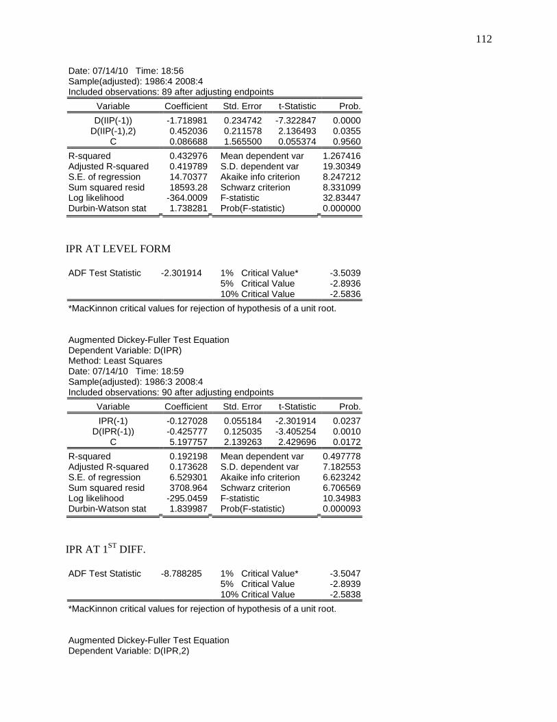
112
Date: 07/14/10 Time: 18:56 Sample(adjusted): 1986:4 2008:4 Included observations: 89 after adjusting endpoints
Variable Coefficient Std. Error t-Statistic Prob.
D(IIP(-1)) -1.718981 0.234742 -7.322847 0.0000 D(IIP(-1),2) 0.452036 0.211578 2.136493 0.0355
C 0.086688 1.565500 0.055374 0.9560
R-squared 0.432976 Mean dependent var 1.267416 Adjusted R-squared 0.419789 S.D. dependent var 19.30349 S.E. of regression 14.70377 Akaike info criterion 8.247212 Sum squared resid 18593.28 Schwarz criterion 8.331099 Log likelihood -364.0009 F-statistic 32.83447 Durbin-Watson stat 1.738281 Prob(F-statistic) 0.000000
IPR AT LEVEL FORM
ADF Test Statistic -2.301914 1% Critical Value* -3.5039
5% Critical Value -2.8936 10% Critical Value -2.5836
*MacKinnon critical values for rejection of hypothesis of a unit root.
Augmented Dickey-Fuller Test Equation Dependent Variable: D(IPR) Method: Least Squares Date: 07/14/10 Time: 18:59 Sample(adjusted): 1986:3 2008:4 Included observations: 90 after adjusting endpoints
Variable Coefficient Std. Error t-Statistic Prob.
IPR(-1) -0.127028 0.055184 -2.301914 0.0237 D(IPR(-1)) -0.425777 0.125035 -3.405254 0.0010
C 5.197757 2.139263 2.429696 0.0172
R-squared 0.192198 Mean dependent var 0.497778 Adjusted R-squared 0.173628 S.D. dependent var 7.182553 S.E. of regression 6.529301 Akaike info criterion 6.623242 Sum squared resid 3708.964 Schwarz criterion 6.706569 Log likelihood -295.0459 F-statistic 10.34983 Durbin-Watson stat 1.839987 Prob(F-statistic) 0.000093
IPR AT 1ST
DIFF.
ADF Test Statistic -8.788285 1% Critical Value* -3.5047
5% Critical Value -2.8939 10% Critical Value -2.5838
*MacKinnon critical values for rejection of hypothesis of a unit root.
Augmented Dickey-Fuller Test Equation Dependent Variable: D(IPR,2)
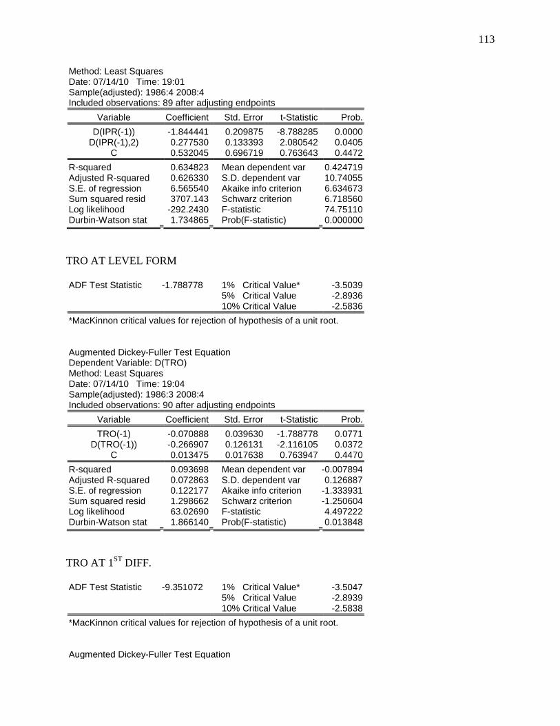
113
Method: Least Squares Date: 07/14/10 Time: 19:01 Sample(adjusted): 1986:4 2008:4 Included observations: 89 after adjusting endpoints
Variable Coefficient Std. Error t-Statistic Prob.
D(IPR(-1)) -1.844441 0.209875 -8.788285 0.0000 D(IPR(-1),2) 0.277530 0.133393 2.080542 0.0405
C 0.532045 0.696719 0.763643 0.4472
R-squared 0.634823 Mean dependent var 0.424719 Adjusted R-squared 0.626330 S.D. dependent var 10.74055 S.E. of regression 6.565540 Akaike info criterion 6.634673 Sum squared resid 3707.143 Schwarz criterion 6.718560 Log likelihood -292.2430 F-statistic 74.75110 Durbin-Watson stat 1.734865 Prob(F-statistic) 0.000000
TRO AT LEVEL FORM
ADF Test Statistic -1.788778 1% Critical Value* -3.5039
5% Critical Value -2.8936 10% Critical Value -2.5836
*MacKinnon critical values for rejection of hypothesis of a unit root.
Augmented Dickey-Fuller Test Equation Dependent Variable: D(TRO) Method: Least Squares Date: 07/14/10 Time: 19:04 Sample(adjusted): 1986:3 2008:4 Included observations: 90 after adjusting endpoints
Variable Coefficient Std. Error t-Statistic Prob.
TRO(-1) -0.070888 0.039630 -1.788778 0.0771 D(TRO(-1)) -0.266907 0.126131 -2.116105 0.0372
C 0.013475 0.017638 0.763947 0.4470
R-squared 0.093698 Mean dependent var -0.007894 Adjusted R-squared 0.072863 S.D. dependent var 0.126887 S.E. of regression 0.122177 Akaike info criterion -1.333931 Sum squared resid 1.298662 Schwarz criterion -1.250604 Log likelihood 63.02690 F-statistic 4.497222 Durbin-Watson stat 1.866140 Prob(F-statistic) 0.013848
TRO AT 1ST
DIFF.
ADF Test Statistic -9.351072 1% Critical Value* -3.5047
5% Critical Value -2.8939 10% Critical Value -2.5838
*MacKinnon critical values for rejection of hypothesis of a unit root.
Augmented Dickey-Fuller Test Equation
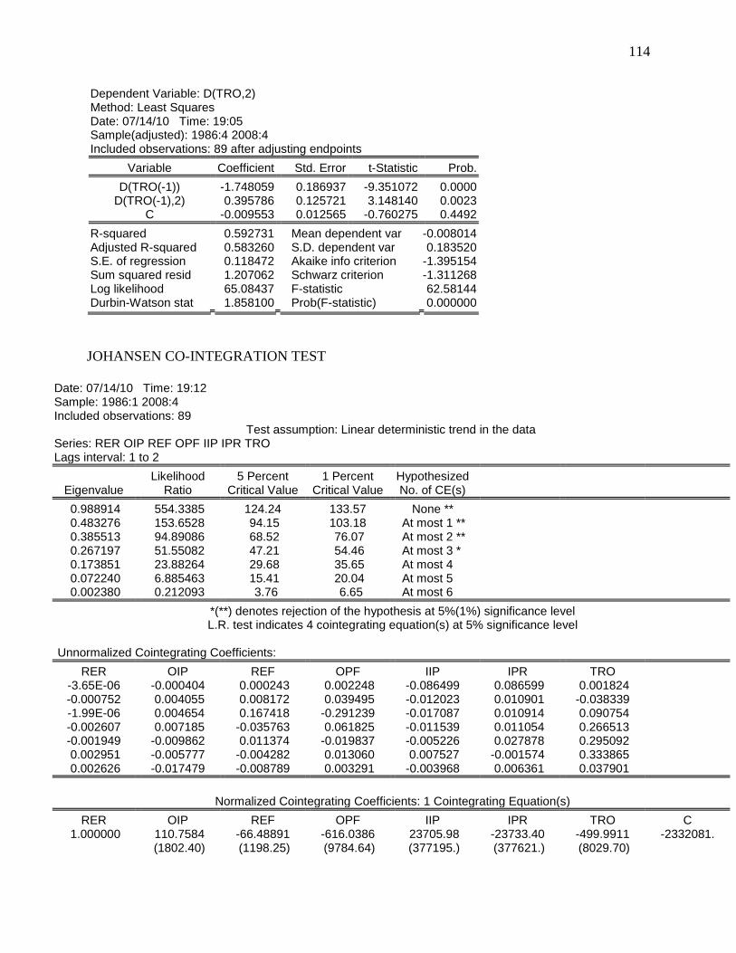
114
Dependent Variable: D(TRO,2) Method: Least Squares Date: 07/14/10 Time: 19:05 Sample(adjusted): 1986:4 2008:4 Included observations: 89 after adjusting endpoints
Variable Coefficient Std. Error t-Statistic Prob.
D(TRO(-1)) -1.748059 0.186937 -9.351072 0.0000 D(TRO(-1),2) 0.395786 0.125721 3.148140 0.0023
C -0.009553 0.012565 -0.760275 0.4492
R-squared 0.592731 Mean dependent var -0.008014 Adjusted R-squared 0.583260 S.D. dependent var 0.183520 S.E. of regression 0.118472 Akaike info criterion -1.395154 Sum squared resid 1.207062 Schwarz criterion -1.311268 Log likelihood 65.08437 F-statistic 62.58144 Durbin-Watson stat 1.858100 Prob(F-statistic) 0.000000
JOHANSEN CO-INTEGRATION TEST
Date: 07/14/10 Time: 19:12 Sample: 1986:1 2008:4 Included observations: 89
Test assumption: Linear deterministic trend in the data Series: RER OIP REF OPF IIP IPR TRO Lags interval: 1 to 2
Likelihood 5 Percent 1 Percent Hypothesized Eigenvalue Ratio Critical Value Critical Value No. of CE(s)
0.988914 554.3385 124.24 133.57 None ** 0.483276 153.6528 94.15 103.18 At most 1 ** 0.385513 94.89086 68.52 76.07 At most 2 ** 0.267197 51.55082 47.21 54.46 At most 3 * 0.173851 23.88264 29.68 35.65 At most 4 0.072240 6.885463 15.41 20.04 At most 5 0.002380 0.212093 3.76 6.65 At most 6
*(**) denotes rejection of the hypothesis at 5%(1%) significance level L.R. test indicates 4 cointegrating equation(s) at 5% significance level
Unnormalized Cointegrating Coefficients:
RER OIP REF OPF IIP IPR TRO -3.65E-06 -0.000404 0.000243 0.002248 -0.086499 0.086599 0.001824 -0.000752 0.004055 0.008172 0.039495 -0.012023 0.010901 -0.038339 -1.99E-06 0.004654 0.167418 -0.291239 -0.017087 0.010914 0.090754 -0.002607 0.007185 -0.035763 0.061825 -0.011539 0.011054 0.266513 -0.001949 -0.009862 0.011374 -0.019837 -0.005226 0.027878 0.295092 0.002951 -0.005777 -0.004282 0.013060 0.007527 -0.001574 0.333865 0.002626 -0.017479 -0.008789 0.003291 -0.003968 0.006361 0.037901
Normalized Cointegrating Coefficients: 1 Cointegrating Equation(s)
RER OIP REF OPF IIP IPR TRO C 1.000000 110.7584 -66.48891 -616.0386 23705.98 -23733.40 -499.9911 -2332081.
(1802.40) (1198.25) (9784.64) (377195.) (377621.) (8029.70)
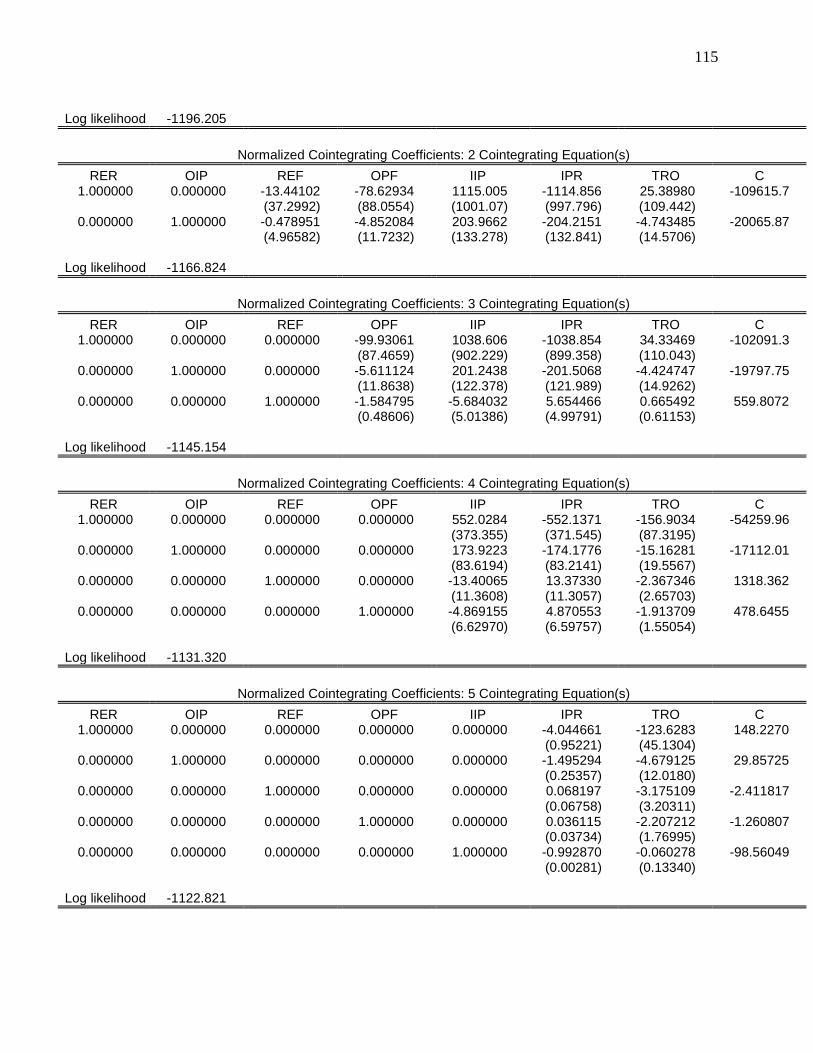
115
Log likelihood -1196.205
Normalized Cointegrating Coefficients: 2 Cointegrating Equation(s)
RER OIP REF OPF IIP IPR TRO C 1.000000 0.000000 -13.44102 -78.62934 1115.005 -1114.856 25.38980 -109615.7
(37.2992) (88.0554) (1001.07) (997.796) (109.442) 0.000000 1.000000 -0.478951 -4.852084 203.9662 -204.2151 -4.743485 -20065.87
(4.96582) (11.7232) (133.278) (132.841) (14.5706)
Log likelihood -1166.824
Normalized Cointegrating Coefficients: 3 Cointegrating Equation(s)
RER OIP REF OPF IIP IPR TRO C 1.000000 0.000000 0.000000 -99.93061 1038.606 -1038.854 34.33469 -102091.3
(87.4659) (902.229) (899.358) (110.043) 0.000000 1.000000 0.000000 -5.611124 201.2438 -201.5068 -4.424747 -19797.75
(11.8638) (122.378) (121.989) (14.9262) 0.000000 0.000000 1.000000 -1.584795 -5.684032 5.654466 0.665492 559.8072
(0.48606) (5.01386) (4.99791) (0.61153)
Log likelihood -1145.154
Normalized Cointegrating Coefficients: 4 Cointegrating Equation(s)
RER OIP REF OPF IIP IPR TRO C 1.000000 0.000000 0.000000 0.000000 552.0284 -552.1371 -156.9034 -54259.96
(373.355) (371.545) (87.3195) 0.000000 1.000000 0.000000 0.000000 173.9223 -174.1776 -15.16281 -17112.01
(83.6194) (83.2141) (19.5567) 0.000000 0.000000 1.000000 0.000000 -13.40065 13.37330 -2.367346 1318.362
(11.3608) (11.3057) (2.65703) 0.000000 0.000000 0.000000 1.000000 -4.869155 4.870553 -1.913709 478.6455
(6.62970) (6.59757) (1.55054)
Log likelihood -1131.320
Normalized Cointegrating Coefficients: 5 Cointegrating Equation(s)
RER OIP REF OPF IIP IPR TRO C 1.000000 0.000000 0.000000 0.000000 0.000000 -4.044661 -123.6283 148.2270
(0.95221) (45.1304) 0.000000 1.000000 0.000000 0.000000 0.000000 -1.495294 -4.679125 29.85725
(0.25357) (12.0180) 0.000000 0.000000 1.000000 0.000000 0.000000 0.068197 -3.175109 -2.411817
(0.06758) (3.20311) 0.000000 0.000000 0.000000 1.000000 0.000000 0.036115 -2.207212 -1.260807
(0.03734) (1.76995) 0.000000 0.000000 0.000000 0.000000 1.000000 -0.992870 -0.060278 -98.56049
(0.00281) (0.13340)
Log likelihood -1122.821
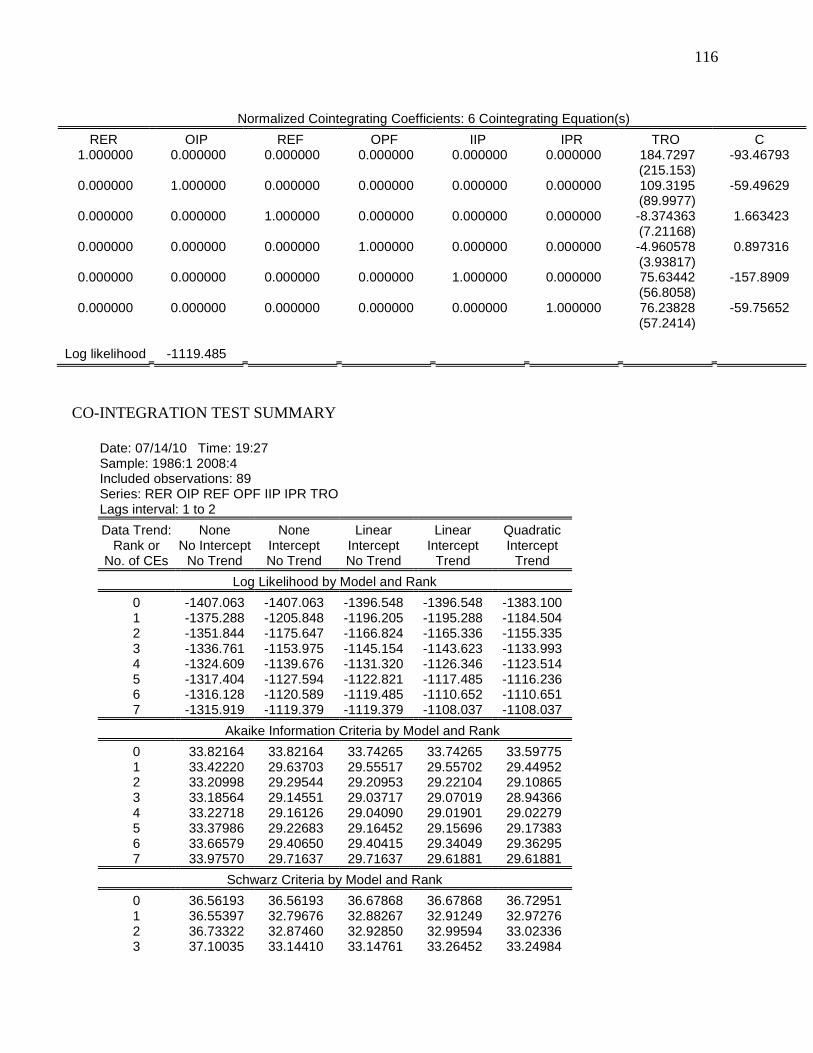
116
Normalized Cointegrating Coefficients: 6 Cointegrating Equation(s)
RER OIP REF OPF IIP IPR TRO C 1.000000 0.000000 0.000000 0.000000 0.000000 0.000000 184.7297 -93.46793
(215.153) 0.000000 1.000000 0.000000 0.000000 0.000000 0.000000 109.3195 -59.49629
(89.9977) 0.000000 0.000000 1.000000 0.000000 0.000000 0.000000 -8.374363 1.663423
(7.21168) 0.000000 0.000000 0.000000 1.000000 0.000000 0.000000 -4.960578 0.897316
(3.93817) 0.000000 0.000000 0.000000 0.000000 1.000000 0.000000 75.63442 -157.8909
(56.8058) 0.000000 0.000000 0.000000 0.000000 0.000000 1.000000 76.23828 -59.75652
(57.2414)
Log likelihood -1119.485
CO-INTEGRATION TEST SUMMARY
Date: 07/14/10 Time: 19:27 Sample: 1986:1 2008:4 Included observations: 89 Series: RER OIP REF OPF IIP IPR TRO Lags interval: 1 to 2
Data Trend: None None Linear Linear Quadratic Rank or No Intercept Intercept Intercept Intercept Intercept
No. of CEs No Trend No Trend No Trend Trend Trend
Log Likelihood by Model and Rank
0 -1407.063 -1407.063 -1396.548 -1396.548 -1383.100 1 -1375.288 -1205.848 -1196.205 -1195.288 -1184.504 2 -1351.844 -1175.647 -1166.824 -1165.336 -1155.335 3 -1336.761 -1153.975 -1145.154 -1143.623 -1133.993 4 -1324.609 -1139.676 -1131.320 -1126.346 -1123.514 5 -1317.404 -1127.594 -1122.821 -1117.485 -1116.236 6 -1316.128 -1120.589 -1119.485 -1110.652 -1110.651 7 -1315.919 -1119.379 -1119.379 -1108.037 -1108.037
Akaike Information Criteria by Model and Rank
0 33.82164 33.82164 33.74265 33.74265 33.59775 1 33.42220 29.63703 29.55517 29.55702 29.44952 2 33.20998 29.29544 29.20953 29.22104 29.10865 3 33.18564 29.14551 29.03717 29.07019 28.94366 4 33.22718 29.16126 29.04090 29.01901 29.02279 5 33.37986 29.22683 29.16452 29.15696 29.17383 6 33.66579 29.40650 29.40415 29.34049 29.36295 7 33.97570 29.71637 29.71637 29.61881 29.61881
Schwarz Criteria by Model and Rank
0 36.56193 36.56193 36.67868 36.67868 36.72951 1 36.55397 32.79676 32.88267 32.91249 32.97276 2 36.73322 32.87460 32.92850 32.99594 33.02336 3 37.10035 33.14410 33.14761 33.26452 33.24984
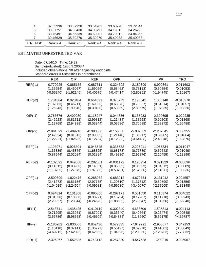
117
4 37.53336 33.57928 33.54281 33.63278 33.72044 5 38.07751 34.06430 34.05791 34.19015 34.26295 6 38.75491 34.66339 34.68901 34.79312 34.84355 7 39.45629 35.39270 35.39270 35.49088 35.49088
L.R. Test: Rank = 4 Rank = 5 Rank = 4 Rank = 4 Rank = 3
ESTIMATED UNRESTRICTED VAR
Date: 07/14/10 Time: 19:32 Sample(adjusted): 1986:3 2008:4 Included observations: 90 after adjusting endpoints Standard errors & t-statistics in parentheses
RER OIP REF OPF IIP IPR TRO
RER(-1) -0.770225 -0.885156 -0.687511 -0.324602 -2.189899 -0.990361 0.011603 (1.36954) (0.46067) (1.69026) (0.68462) (0.78113) (0.50854) (0.01053) (-0.56240) (-1.92146) (-0.40675) (-0.47414) (-2.80352) (-1.94745) (1.10167)
RER(-2) 1.734364 0.923484 0.664321 0.370773 2.198541 1.005148 -0.010970 (1.37383) (0.46211) (1.69556) (0.68676) (0.78357) (0.51014) (0.01057) (1.26243) (1.99840) (0.39180) (0.53989) (2.80579) (1.97035) (-1.03826)
OIP(-1) 2.763676 2.409980 0.118247 0.044886 5.135983 2.329695 -0.029235 (2.42923) (0.81711) (2.99812) (1.21434) (1.38553) (0.90203) (0.01868) (1.13768) (2.94938) (0.03944) (0.03696) (3.70688) (2.58272) (-1.56488)
OIP(-2) -2.961829 -1.489218 -0.380850 -0.156068 -5.037839 -2.232045 0.030355 (2.42334) (0.81513) (2.99085) (1.21140) (1.38217) (0.89985) (0.01864) (-1.22221) (-1.82696) (-0.12734) (-0.12883) (-3.64488) (-2.48048) (1.62876)
REF(-1) 1.193971 0.926801 0.048545 0.335682 2.296911 1.065834 -0.011947 (1.36386) (0.45876) (1.68325) (0.68178) (0.77789) (0.50643) (0.01049) (0.87544) (2.02024) (0.02884) (0.49236) (2.95276) (2.10459) (-1.13899)
REF(-2) -0.132092 0.049868 -0.282801 -0.031172 0.170254 0.091329 -0.000896 (0.11612) (0.03906) (0.14331) (0.05805) (0.06623) (0.04312) (0.00089) (-1.13755) (1.27675) (-1.97330) (-0.53701) (2.57066) (2.11811) (-1.00336)
OPF(-1) -2.509699 -1.822476 -0.288262 -0.683012 -4.679754 -2.131942 0.024557 (2.41273) (0.81156) (2.97775) (1.20610) (1.37612) (0.89590) (0.01856) (-1.04019) (-2.24564) (-0.09681) (-0.56630) (-3.40070) (-2.37965) (1.32348)
OPF(-2) 0.694814 0.131368 -0.095856 -0.297171 0.501550 0.110374 -0.004022 (0.31536) (0.10608) (0.38921) (0.15764) (0.17987) (0.11710) (0.00243) (2.20327) (1.23844) (-0.24629) (-1.88509) (2.78847) (0.94256) (-1.65840)
IIP(-1) 2.543711 1.435425 -0.410119 -0.302349 4.633609 1.506813 -0.024113 (0.71295) (0.23981) (0.87991) (0.35640) (0.40664) (0.26474) (0.00548) (3.56786) (5.98558) (-0.46609) (-0.84835) (11.3950) (5.69175) (-4.39787)
IIP(-2) -5.180982 -2.830506 0.852436 0.577335 -7.642991 -2.955077 0.049153 (1.10418) (0.37141) (1.36277) (0.55197) (0.62978) (0.41001) (0.00849) (-4.69215) (-7.62095) (0.62552) (1.04596) (-12.1360) (-7.20733) (5.78832)
IPR(-1) -2.326267 -1.552835 0.743112 0.257320 -4.547588 -1.293219 0.025967
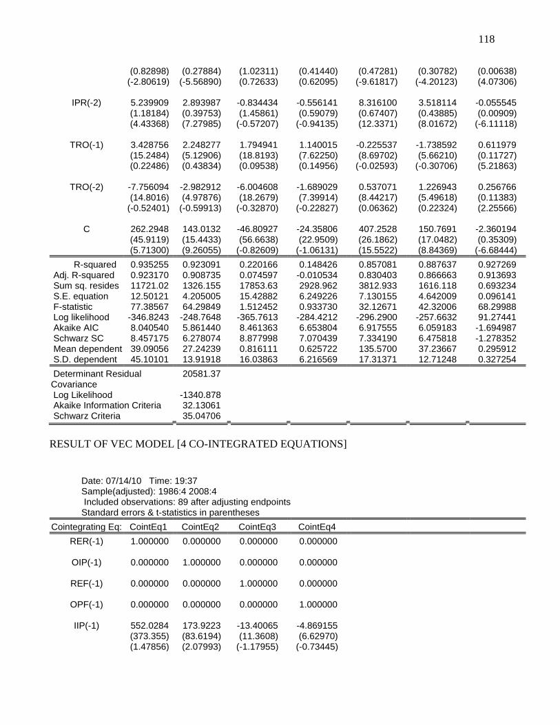
118
(0.82898) (0.27884) (1.02311) (0.41440) (0.47281) (0.30782) (0.00638) (-2.80619) (-5.56890) (0.72633) (0.62095) (-9.61817) (-4.20123) (4.07306)
IPR(-2) 5.239909 2.893987 -0.834434 -0.556141 8.316100 3.518114 -0.055545 (1.18184) (0.39753) (1.45861) (0.59079) (0.67407) (0.43885) (0.00909) (4.43368) (7.27985) (-0.57207) (-0.94135) (12.3371) (8.01672) (-6.11118)
TRO(-1) 3.428756 2.248277 1.794941 1.140015 -0.225537 -1.738592 0.611979 (15.2484) (5.12906) (18.8193) (7.62250) (8.69702) (5.66210) (0.11727) (0.22486) (0.43834) (0.09538) (0.14956) (-0.02593) (-0.30706) (5.21863)
TRO(-2) -7.756094 -2.982912 -6.004608 -1.689029 0.537071 1.226943 0.256766 (14.8016) (4.97876) (18.2679) (7.39914) (8.44217) (5.49618) (0.11383) (-0.52401) (-0.59913) (-0.32870) (-0.22827) (0.06362) (0.22324) (2.25566)
C 262.2948 143.0132 -46.80927 -24.35806 407.2528 150.7691 -2.360194 (45.9119) (15.4433) (56.6638) (22.9509) (26.1862) (17.0482) (0.35309) (5.71300) (9.26055) (-0.82609) (-1.06131) (15.5522) (8.84369) (-6.68444)
R-squared 0.935255 0.923091 0.220166 0.148426 0.857081 0.887637 0.927269 Adj. R-squared 0.923170 0.908735 0.074597 -0.010534 0.830403 0.866663 0.913693 Sum sq. resides 11721.02 1326.155 17853.63 2928.962 3812.933 1616.118 0.693234 S.E. equation 12.50121 4.205005 15.42882 6.249226 7.130155 4.642009 0.096141 F-statistic 77.38567 64.29849 1.512452 0.933730 32.12671 42.32006 68.29988 Log likelihood -346.8243 -248.7648 -365.7613 -284.4212 -296.2900 -257.6632 91.27441 Akaike AIC 8.040540 5.861440 8.461363 6.653804 6.917555 6.059183 -1.694987 Schwarz SC 8.457175 6.278074 8.877998 7.070439 7.334190 6.475818 -1.278352 Mean dependent 39.09056 27.24239 0.816111 0.625722 135.5700 37.23667 0.295912 S.D. dependent 45.10101 13.91918 16.03863 6.216569 17.31371 12.71248 0.327254
Determinant Residual Covariance
20581.37
Log Likelihood -1340.878 Akaike Information Criteria 32.13061 Schwarz Criteria 35.04706
RESULT OF VEC MODEL [4 CO-INTEGRATED EQUATIONS]
Date: 07/14/10 Time: 19:37 Sample(adjusted): 1986:4 2008:4 Included observations: 89 after adjusting endpoints Standard errors & t-statistics in parentheses
Cointegrating Eq: CointEq1 CointEq2 CointEq3 CointEq4
RER(-1) 1.000000 0.000000 0.000000 0.000000
OIP(-1) 0.000000 1.000000 0.000000 0.000000
REF(-1) 0.000000 0.000000 1.000000 0.000000
OPF(-1) 0.000000 0.000000 0.000000 1.000000
IIP(-1) 552.0284 173.9223 -13.40065 -4.869155 (373.355) (83.6194) (11.3608) (6.62970) (1.47856) (2.07993) (-1.17955) (-0.73445)
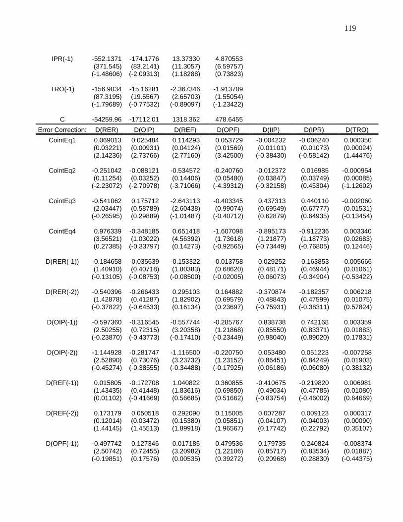
119
IPR(-1) -552.1371 -174.1776 13.37330 4.870553
(371.545) (83.2141) (11.3057) (6.59757) (-1.48606) (-2.09313) (1.18288) (0.73823)
TRO(-1) -156.9034 -15.16281 -2.367346 -1.913709 (87.3195) (19.5567) (2.65703) (1.55054) (-1.79689) (-0.77532) (-0.89097) (-1.23422)
C -54259.96 -17112.01 1318.362 478.6455
Error Correction: D(RER) D(OIP) D(REF) D(OPF) D(IIP) D(IPR) D(TRO)
CointEq1 0.069013 0.025484 0.114293 0.053729 -0.004232 -0.006240 0.000350 (0.03221) (0.00931) (0.04124) (0.01569) (0.01101) (0.01073) (0.00024) (2.14236) (2.73766) (2.77160) (3.42500) (-0.38430) (-0.58142) (1.44476)
CointEq2 -0.251042 -0.088121 -0.534572 -0.240760 -0.012372 0.016985 -0.000954 (0.11254) (0.03252) (0.14406) (0.05480) (0.03847) (0.03749) (0.00085) (-2.23072) (-2.70978) (-3.71066) (-4.39312) (-0.32158) (0.45304) (-1.12602)
CointEq3 -0.541062 0.175712 -2.643113 -0.403345 0.437313 0.440110 -0.002060 (2.03447) (0.58789) (2.60438) (0.99074) (0.69549) (0.67777) (0.01531) (-0.26595) (0.29889) (-1.01487) (-0.40712) (0.62879) (0.64935) (-0.13454)
CointEq4 0.976339 -0.348185 0.651418 -1.607098 -0.895173 -0.912236 0.003340 (3.56521) (1.03022) (4.56392) (1.73618) (1.21877) (1.18773) (0.02683) (0.27385) (-0.33797) (0.14273) (-0.92565) (-0.73449) (-0.76805) (0.12446)
D(RER(-1)) -0.184658 -0.035639 -0.153322 -0.013758 0.029252 -0.163853 -0.005666 (1.40910) (0.40718) (1.80383) (0.68620) (0.48171) (0.46944) (0.01061) (-0.13105) (-0.08753) (-0.08500) (-0.02005) (0.06073) (-0.34904) (-0.53422)
D(RER(-2)) -0.540396 -0.266433 0.295103 0.164882 -0.370874 -0.182357 0.006218 (1.42878) (0.41287) (1.82902) (0.69579) (0.48843) (0.47599) (0.01075) (-0.37822) (-0.64533) (0.16134) (0.23697) (-0.75931) (-0.38311) (0.57824)
D(OIP(-1)) -0.597360 -0.316545 -0.557744 -0.285767 0.838738 0.742168 0.003359 (2.50255) (0.72315) (3.20358) (1.21868) (0.85550) (0.83371) (0.01883) (-0.23870) (-0.43773) (-0.17410) (-0.23449) (0.98040) (0.89020) (0.17831)
D(OIP(-2)) -1.144928 -0.281747 -1.116500 -0.220750 0.053480 0.051223 -0.007258 (2.52890) (0.73076) (3.23732) (1.23152) (0.86451) (0.84249) (0.01903) (-0.45274) (-0.38555) (-0.34488) (-0.17925) (0.06186) (0.06080) (-0.38132)
D(REF(-1)) 0.015805 -0.172708 1.040822 0.360855 -0.410675 -0.219820 0.006981 (1.43435) (0.41448) (1.83616) (0.69850) (0.49034) (0.47785) (0.01080) (0.01102) (-0.41669) (0.56685) (0.51662) (-0.83754) (-0.46002) (0.64669)
D(REF(-2)) 0.173179 0.050518 0.292090 0.115005 0.007287 0.009123 0.000317 (0.12014) (0.03472) (0.15380) (0.05851) (0.04107) (0.04003) (0.00090) (1.44145) (1.45513) (1.89918) (1.96567) (0.17742) (0.22792) (0.35107)
D(OPF(-1)) -0.497742 0.127346 0.017185 0.479536 0.179735 0.240824 -0.008374 (2.50742) (0.72455) (3.20982) (1.22106) (0.85717) (0.83534) (0.01887) (-0.19851) (0.17576) (0.00535) (0.39272) (0.20968) (0.28830) (-0.44375)
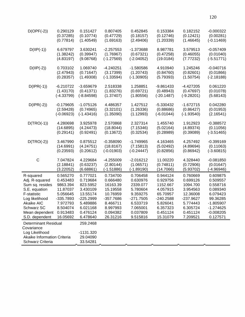
120
D(OPF(-2)) 0.290129 0.151427 0.807405 0.452845 0.153384 0.182152 -0.000322 (0.37285) (0.10774) (0.47729) (0.18157) (0.12746) (0.12421) (0.00281) (0.77814) (1.40549) (1.69163) (2.49406) (1.20339) (1.46645) (-0.11469)
D(IIP(-1)) 6.679797 3.630241 -2.257553 -1.373688 8.987781 3.579513 -0.057409 (1.38242) (0.39947) (1.76967) (0.67321) (0.47258) (0.46055) (0.01040) (4.83197) (9.08768) (-1.27569) (-2.04052) (19.0184) (7.77232) (-5.51771)
D(IIP(-2)) 0.703102 1.069740 -4.240251 -1.580586 4.910940 1.245246 -0.040716 (2.47943) (0.71647) (3.17399) (1.20743) (0.84760) (0.82601) (0.01866) (0.28357) (1.49308) (-1.33594) (-1.30905) (5.79393) (1.50754) (-2.18188)
D(IPR(-1)) -6.210722 -3.659679 2.518338 1.258851 -9.861433 -4.427205 0.061220 (1.43170) (0.41371) (1.83276) (0.69721) (0.48943) (0.47697) (0.01078) (-4.33799) (-8.84598) (1.37407) (1.80556) (-20.1487) (-9.28201) (5.68143)
D(IPR(-2)) -0.179605 -1.075126 4.486357 1.427512 -5.330432 -1.672715 0.042280 (2.59428) (0.74965) (3.32101) (1.26336) (0.88686) (0.86427) (0.01953) (-0.06923) (-1.43416) (1.35090) (1.12993) (-6.01044) (-1.93540) (2.16541)
D(TRO(-1)) 4.280698 3.925978 2.570868 2.327314 1.455740 1.912923 -0.388572 (14.6895) (4.24473) (18.8044) (7.15346) (5.02164) (4.89374) (0.11056) (0.29141) (0.92491) (0.13672) (0.32534) (0.28989) (0.39089) (-3.51465)
D(TRO(-2)) 3.467990 0.875512 -0.358090 -1.749965 4.163465 4.257492 -0.399169 (14.6991) (4.24751) (18.8167) (7.15813) (5.02492) (4.89694) (0.11063) (0.23593) (0.20612) (-0.01903) (-0.24447) (0.82856) (0.86942) (-3.60815)
C 7.047824 4.229684 -4.255009 -2.016212 11.00220 4.328440 -0.081850 (2.18841) (0.63237) (2.80144) (1.06571) (0.74811) (0.72906) (0.01647) (3.22052) (6.68861) (-1.51886) (-1.89190) (14.7066) (5.93702) (-4.96946)
R-squared 0.565270 0.777021 0.734700 0.706458 0.944124 0.760669 0.609875 Adj. R-squared 0.453483 0.719684 0.666480 0.630976 0.929756 0.699126 0.509557 Sum sq. resides 9863.394 823.5952 16163.39 2339.077 1152.667 1094.700 0.558716 S.E. equation 11.87037 3.430109 15.19558 5.780604 4.057915 3.954563 0.089340 F-statistic 5.056645 13.55174 10.76959 9.359275 65.70957 12.36008 6.079423 Log likelihood -335.7893 -225.2999 -357.7686 -271.7505 -240.2588 -237.9627 99.36285 Akaike AIC 7.972793 5.489886 8.466711 6.533719 5.826041 5.774443 -1.805907 Schwarz SC 8.504074 6.021168 8.997993 7.065001 6.357323 6.305724 -1.274625 Mean dependent 0.913483 0.476124 0.094382 0.037809 0.451124 0.451124 -0.008205 S.D. dependent 16.05692 6.478640 26.31216 9.515816 15.31079 7.209521 0.127571
Determinant Residual Covariance
259.2468
Log Likelihood -1131.320 Akaike Information Criteria 29.04090 Schwarz Criteria 33.54281
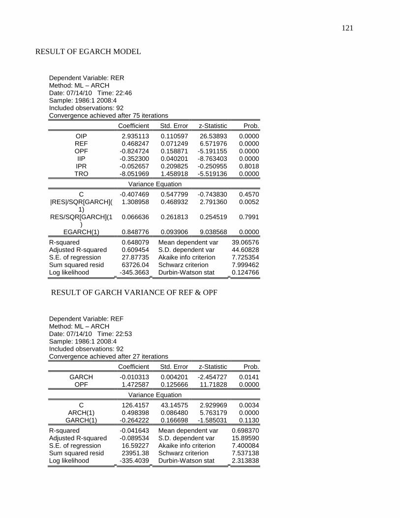
121
RESULT OF EGARCH MODEL
Dependent Variable: RER Method: ML – ARCH Date: 07/14/10 Time: 22:46 Sample: 1986:1 2008:4 Included observations: 92 Convergence achieved after 75 iterations
Coefficient Std. Error z-Statistic Prob.
OIP 2.935113 0.110597 26.53893 0.0000 REF 0.468247 0.071249 6.571976 0.0000 OPF -0.824724 0.158871 -5.191155 0.0000 IIP -0.352300 0.040201 -8.763403 0.0000 IPR -0.052657 0.209825 -0.250955 0.8018 TRO -8.051969 1.458918 -5.519136 0.0000
Variance Equation
C -0.407469 0.547799 -0.743830 0.4570 |RES|/SQR[GARCH](
1) 1.308958 0.468932 2.791360 0.0052
RES/SQR[GARCH](1)
0.066636 0.261813 0.254519 0.7991
EGARCH(1) 0.848776 0.093906 9.038568 0.0000
R-squared 0.648079 Mean dependent var 39.06576 Adjusted R-squared 0.609454 S.D. dependent var 44.60828 S.E. of regression 27.87735 Akaike info criterion 7.725354 Sum squared resid 63726.04 Schwarz criterion 7.999462 Log likelihood -345.3663 Durbin-Watson stat 0.124766
RESULT OF GARCH VARIANCE OF REF & OPF
Dependent Variable: REF Method: ML – ARCH Date: 07/14/10 Time: 22:53 Sample: 1986:1 2008:4 Included observations: 92 Convergence achieved after 27 iterations
Coefficient Std. Error z-Statistic Prob.
GARCH -0.010313 0.004201 -2.454727 0.0141 OPF 1.472587 0.125666 11.71828 0.0000
Variance Equation
C 126.4157 43.14575 2.929969 0.0034 ARCH(1) 0.498398 0.086480 5.763179 0.0000
GARCH(1) -0.264222 0.166698 -1.585031 0.1130
R-squared -0.041643 Mean dependent var 0.698370 Adjusted R-squared -0.089534 S.D. dependent var 15.89590 S.E. of regression 16.59227 Akaike info criterion 7.400084 Sum squared resid 23951.38 Schwarz criterion 7.537138 Log likelihood -335.4039 Durbin-Watson stat 2.313838
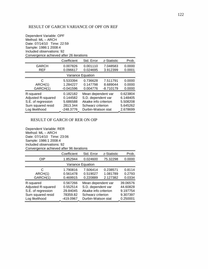
122
RESULT OF GARCH VARIANCE OF OPF ON REF
Dependent Variable: OPF Method: ML – ARCH Date: 07/14/10 Time: 22:59 Sample: 1986:1 2008:4 Included observations: 92 Convergence achieved after 26 iterations
Coefficient Std. Error z-Statistic Prob.
GARCH 0.007826 0.001110 7.048583 0.0000 REF 0.096617 0.024695 3.912399 0.0001
Variance Equation
C 5.533394 0.736628 7.511791 0.0000 ARCH(1) 1.284227 0.147798 8.689044 0.0000
GARCH(1) -0.041596 0.004776 -8.710179 0.0000
R-squared 0.182182 Mean dependent var 0.623804 Adjusted R-squared 0.144582 S.D. dependent var 6.148405 S.E. of regression 5.686588 Akaike info criterion 5.508208 Sum squared resid 2813.344 Schwarz criterion 5.645262 Log likelihood -248.3776 Durbin-Watson stat 2.678699
RESULT OF GARCH OF RER ON OIP
Dependent Variable: RER Method: ML – ARCH Date: 07/14/10 Time: 23:06 Sample: 1986:1 2008:4 Included observations: 92 Convergence achieved after 96 iterations
Coefficient Std. Error z-Statistic Prob.
OIP 1.852944 0.024600 75.32298 0.0000
Variance Equation
C 1.790816 7.506414 0.238571 0.8114 ARCH(1) 0.561478 0.519027 1.081789 0.2793
GARCH(1) 0.469915 0.220889 2.127382 0.0334
R-squared 0.567266 Mean dependent var 39.06576 Adjusted R-squared 0.552514 S.D. dependent var 44.60828 S.E. of regression 29.84045 Akaike info criterion 9.197754 Sum squared resid 78359.82 Schwarz criterion 9.307397 Log likelihood -419.0967 Durbin-Watson stat 0.250001
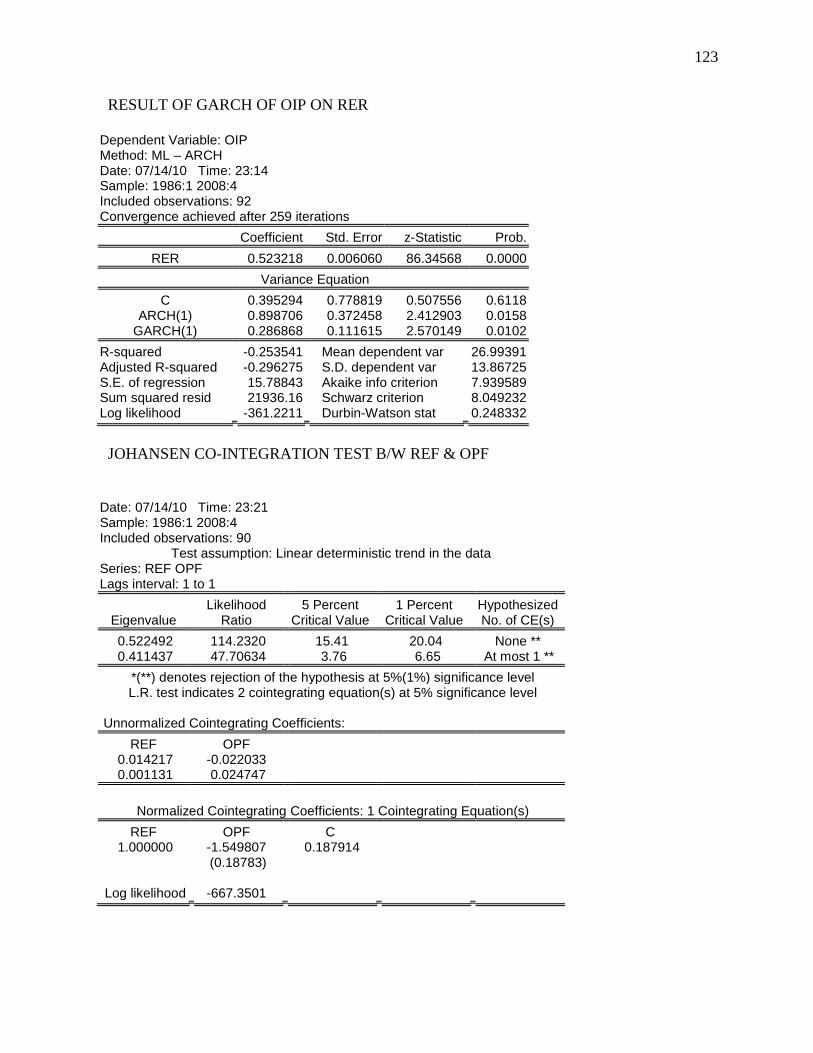
123
RESULT OF GARCH OF OIP ON RER
Dependent Variable: OIP Method: ML – ARCH Date: 07/14/10 Time: 23:14 Sample: 1986:1 2008:4 Included observations: 92 Convergence achieved after 259 iterations
Coefficient Std. Error z-Statistic Prob.
RER 0.523218 0.006060 86.34568 0.0000
Variance Equation
C 0.395294 0.778819 0.507556 0.6118 ARCH(1) 0.898706 0.372458 2.412903 0.0158
GARCH(1) 0.286868 0.111615 2.570149 0.0102
R-squared -0.253541 Mean dependent var 26.99391 Adjusted R-squared -0.296275 S.D. dependent var 13.86725 S.E. of regression 15.78843 Akaike info criterion 7.939589 Sum squared resid 21936.16 Schwarz criterion 8.049232 Log likelihood -361.2211 Durbin-Watson stat 0.248332
JOHANSEN CO-INTEGRATION TEST B/W REF & OPF
Date: 07/14/10 Time: 23:21 Sample: 1986:1 2008:4 Included observations: 90
Test assumption: Linear deterministic trend in the data Series: REF OPF Lags interval: 1 to 1
Likelihood 5 Percent 1 Percent Hypothesized Eigenvalue Ratio Critical Value Critical Value No. of CE(s)
0.522492 114.2320 15.41 20.04 None ** 0.411437 47.70634 3.76 6.65 At most 1 **
*(**) denotes rejection of the hypothesis at 5%(1%) significance level L.R. test indicates 2 cointegrating equation(s) at 5% significance level
Unnormalized Cointegrating Coefficients:
REF OPF 0.014217 -0.022033 0.001131 0.024747
Normalized Cointegrating Coefficients: 1 Cointegrating Equation(s)
REF OPF C 1.000000 -1.549807 0.187914
(0.18783)
Log likelihood -667.3501
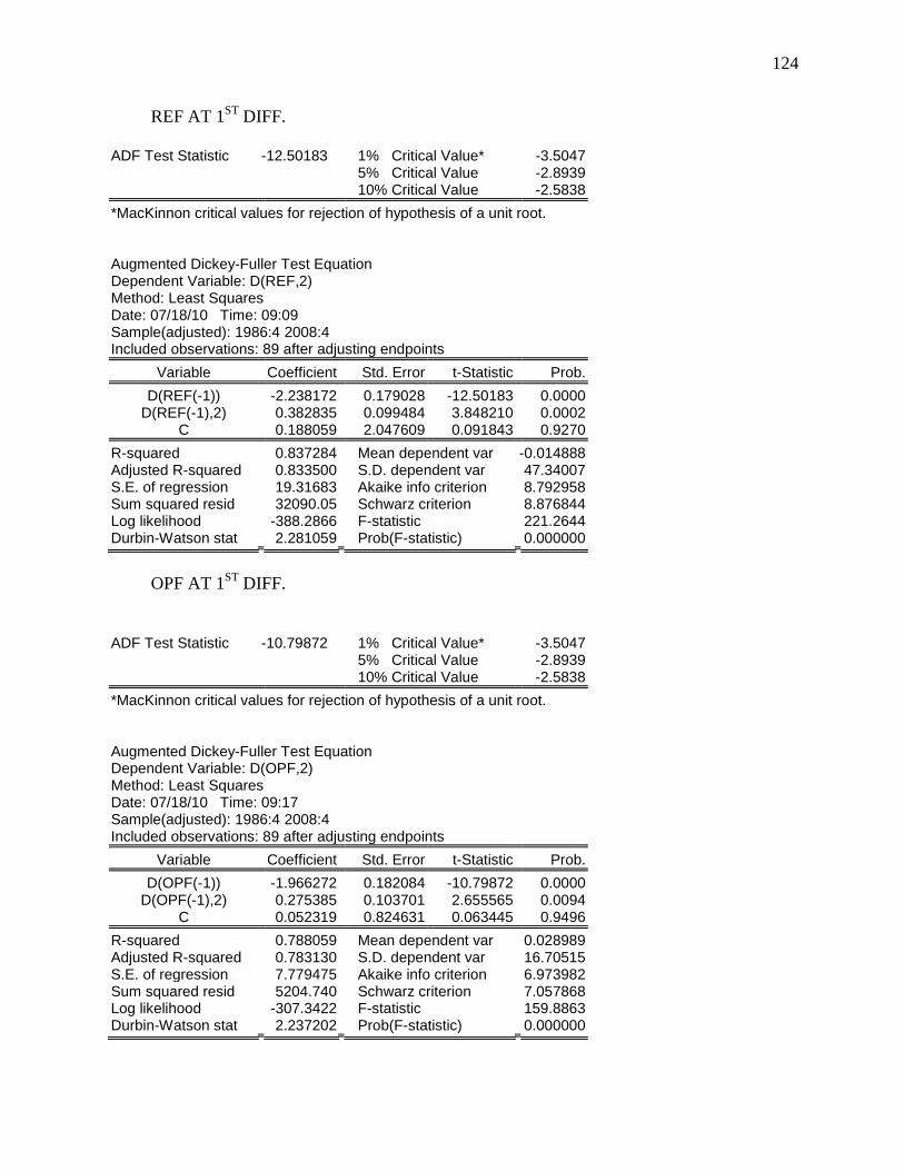
124
REF AT 1ST
DIFF.
ADF Test Statistic -12.50183 1% Critical Value* -3.5047
5% Critical Value -2.8939 10% Critical Value -2.5838
*MacKinnon critical values for rejection of hypothesis of a unit root.
Augmented Dickey-Fuller Test Equation Dependent Variable: D(REF,2) Method: Least Squares Date: 07/18/10 Time: 09:09 Sample(adjusted): 1986:4 2008:4 Included observations: 89 after adjusting endpoints
Variable Coefficient Std. Error t-Statistic Prob.
D(REF(-1)) -2.238172 0.179028 -12.50183 0.0000 D(REF(-1),2) 0.382835 0.099484 3.848210 0.0002
C 0.188059 2.047609 0.091843 0.9270
R-squared 0.837284 Mean dependent var -0.014888 Adjusted R-squared 0.833500 S.D. dependent var 47.34007 S.E. of regression 19.31683 Akaike info criterion 8.792958 Sum squared resid 32090.05 Schwarz criterion 8.876844 Log likelihood -388.2866 F-statistic 221.2644 Durbin-Watson stat 2.281059 Prob(F-statistic) 0.000000
OPF AT 1ST
DIFF.
ADF Test Statistic -10.79872 1% Critical Value* -3.5047
5% Critical Value -2.8939 10% Critical Value -2.5838
*MacKinnon critical values for rejection of hypothesis of a unit root.
Augmented Dickey-Fuller Test Equation Dependent Variable: D(OPF,2) Method: Least Squares Date: 07/18/10 Time: 09:17 Sample(adjusted): 1986:4 2008:4 Included observations: 89 after adjusting endpoints
Variable Coefficient Std. Error t-Statistic Prob.
D(OPF(-1)) -1.966272 0.182084 -10.79872 0.0000 D(OPF(-1),2) 0.275385 0.103701 2.655565 0.0094
C 0.052319 0.824631 0.063445 0.9496
R-squared 0.788059 Mean dependent var 0.028989 Adjusted R-squared 0.783130 S.D. dependent var 16.70515 S.E. of regression 7.779475 Akaike info criterion 6.973982 Sum squared resid 5204.740 Schwarz criterion 7.057868 Log likelihood -307.3422 F-statistic 159.8863 Durbin-Watson stat 2.237202 Prob(F-statistic) 0.000000
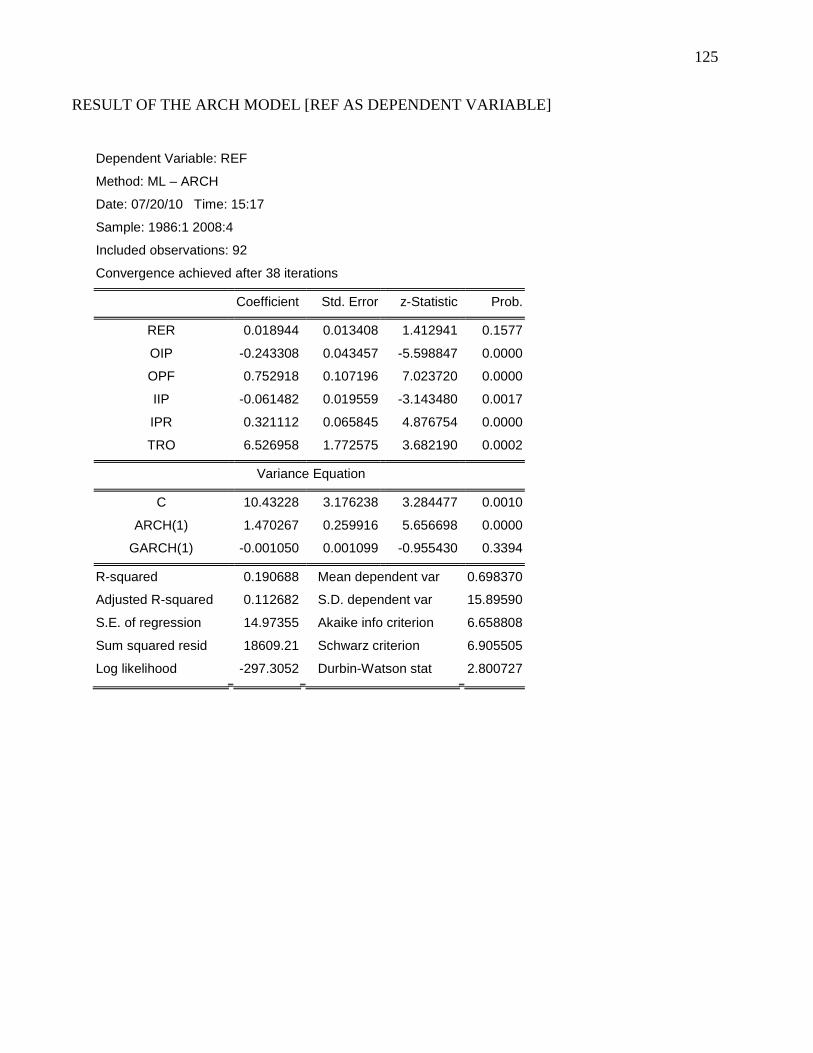
125
RESULT OF THE ARCH MODEL [REF AS DEPENDENT VARIABLE]
Dependent Variable: REF
Method: ML – ARCH
Date: 07/20/10 Time: 15:17
Sample: 1986:1 2008:4
Included observations: 92
Convergence achieved after 38 iterations
Coefficient Std. Error z-Statistic Prob.
RER 0.018944 0.013408 1.412941 0.1577
OIP -0.243308 0.043457 -5.598847 0.0000
OPF 0.752918 0.107196 7.023720 0.0000
IIP -0.061482 0.019559 -3.143480 0.0017
IPR 0.321112 0.065845 4.876754 0.0000
TRO 6.526958 1.772575 3.682190 0.0002
Variance Equation
C 10.43228 3.176238 3.284477 0.0010
ARCH(1) 1.470267 0.259916 5.656698 0.0000
GARCH(1) -0.001050 0.001099 -0.955430 0.3394
R-squared 0.190688 Mean dependent var 0.698370
Adjusted R-squared 0.112682 S.D. dependent var 15.89590
S.E. of regression 14.97355 Akaike info criterion 6.658808
Sum squared resid 18609.21 Schwarz criterion 6.905505
Log likelihood -297.3052 Durbin-Watson stat 2.800727
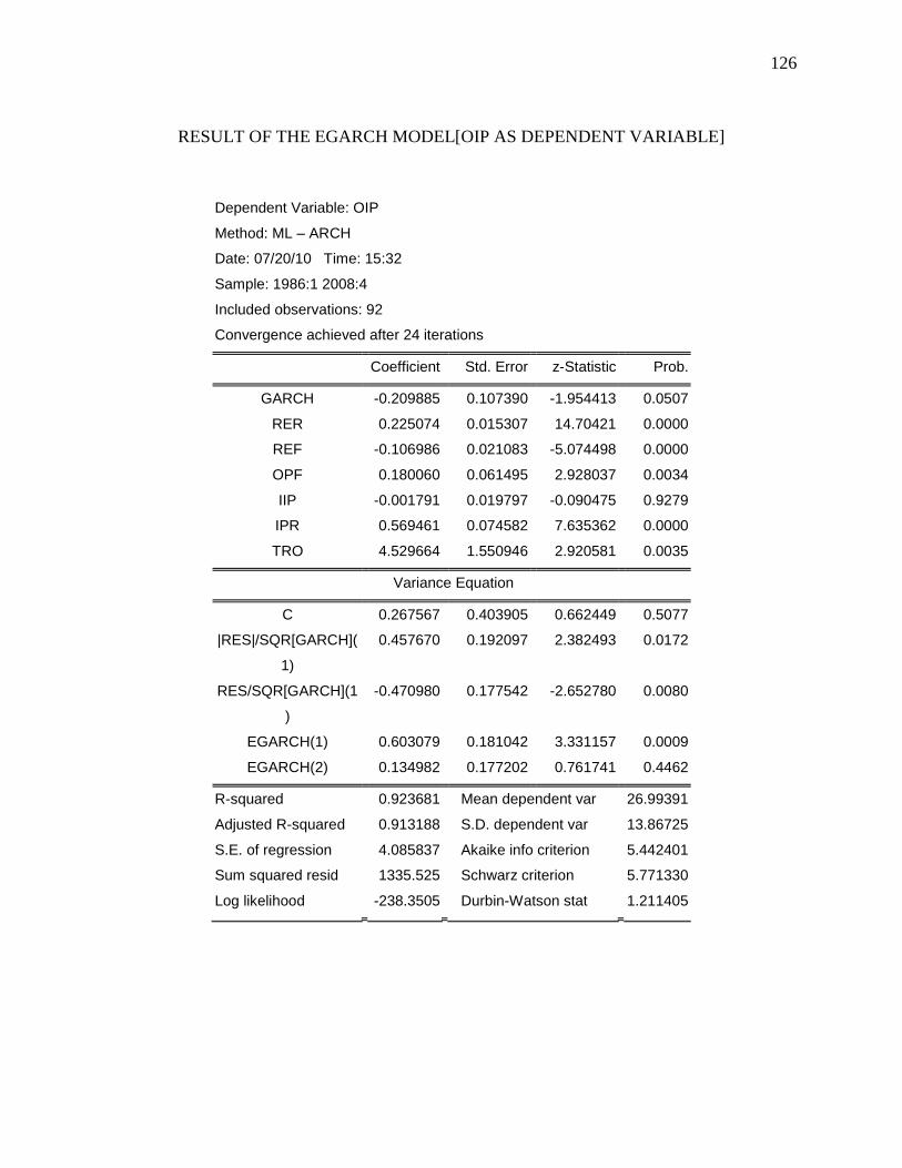
126
RESULT OF THE EGARCH MODEL[OIP AS DEPENDENT VARIABLE]
Dependent Variable: OIP
Method: ML – ARCH
Date: 07/20/10 Time: 15:32
Sample: 1986:1 2008:4
Included observations: 92
Convergence achieved after 24 iterations
Coefficient Std. Error z-Statistic Prob.
GARCH -0.209885 0.107390 -1.954413 0.0507
RER 0.225074 0.015307 14.70421 0.0000
REF -0.106986 0.021083 -5.074498 0.0000
OPF 0.180060 0.061495 2.928037 0.0034
IIP -0.001791 0.019797 -0.090475 0.9279
IPR 0.569461 0.074582 7.635362 0.0000
TRO 4.529664 1.550946 2.920581 0.0035
Variance Equation
C 0.267567 0.403905 0.662449 0.5077
|RES|/SQR[GARCH](
1)
0.457670 0.192097 2.382493 0.0172
RES/SQR[GARCH](1
)
-0.470980 0.177542 -2.652780 0.0080
EGARCH(1) 0.603079 0.181042 3.331157 0.0009
EGARCH(2) 0.134982 0.177202 0.761741 0.4462
R-squared 0.923681 Mean dependent var 26.99391
Adjusted R-squared 0.913188 S.D. dependent var 13.86725
S.E. of regression 4.085837 Akaike info criterion 5.442401
Sum squared resid 1335.525 Schwarz criterion 5.771330
Log likelihood -238.3505 Durbin-Watson stat 1.211405
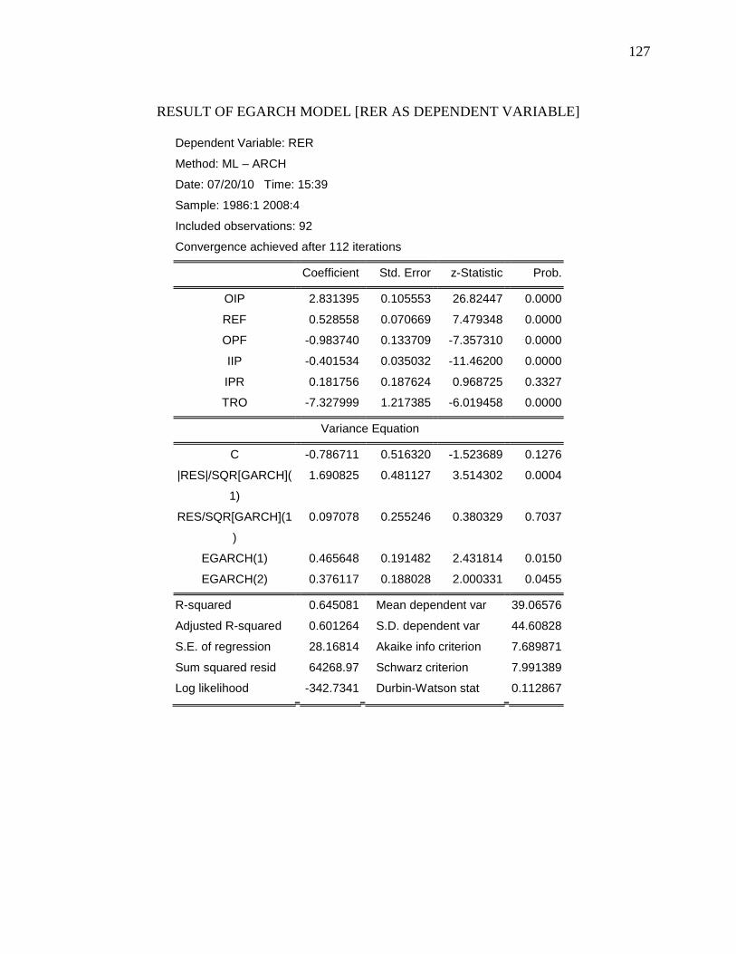
127
RESULT OF EGARCH MODEL [RER AS DEPENDENT VARIABLE]
Dependent Variable: RER
Method: ML – ARCH
Date: 07/20/10 Time: 15:39
Sample: 1986:1 2008:4
Included observations: 92
Convergence achieved after 112 iterations
Coefficient Std. Error z-Statistic Prob.
OIP 2.831395 0.105553 26.82447 0.0000
REF 0.528558 0.070669 7.479348 0.0000
OPF -0.983740 0.133709 -7.357310 0.0000
IIP -0.401534 0.035032 -11.46200 0.0000
IPR 0.181756 0.187624 0.968725 0.3327
TRO -7.327999 1.217385 -6.019458 0.0000
Variance Equation
C -0.786711 0.516320 -1.523689 0.1276
|RES|/SQR[GARCH](
1)
1.690825 0.481127 3.514302 0.0004
RES/SQR[GARCH](1
)
0.097078 0.255246 0.380329 0.7037
EGARCH(1) 0.465648 0.191482 2.431814 0.0150
EGARCH(2) 0.376117 0.188028 2.000331 0.0455
R-squared 0.645081 Mean dependent var 39.06576
Adjusted R-squared 0.601264 S.D. dependent var 44.60828
S.E. of regression 28.16814 Akaike info criterion 7.689871
Sum squared resid 64268.97 Schwarz criterion 7.991389
Log likelihood -342.7341 Durbin-Watson stat 0.112867
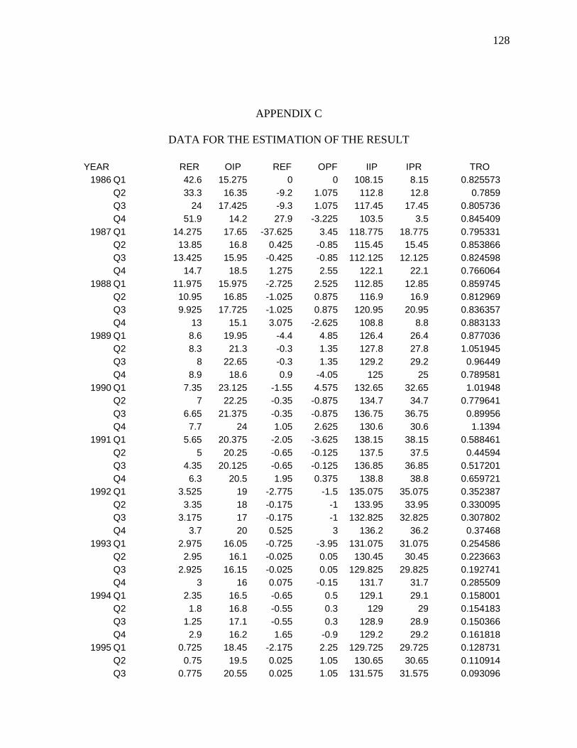
128
APPENDIX C
DATA FOR THE ESTIMATION OF THE RESULT
YEAR RER OIP REF OPF IIP IPR TRO
1986 Q1 42.6 15.275 0 0 108.15 8.15 0.825573
Q2 33.3 16.35 -9.2 1.075 112.8 12.8 0.7859
Q3 24 17.425 -9.3 1.075 117.45 17.45 0.805736
Q4 51.9 14.2 27.9 -3.225 103.5 3.5 0.845409
1987 Q1 14.275 17.65 -37.625 3.45 118.775 18.775 0.795331
Q2 13.85 16.8 0.425 -0.85 115.45 15.45 0.853866
Q3 13.425 15.95 -0.425 -0.85 112.125 12.125 0.824598
Q4 14.7 18.5 1.275 2.55 122.1 22.1 0.766064
1988 Q1 11.975 15.975 -2.725 2.525 112.85 12.85 0.859745
Q2 10.95 16.85 -1.025 0.875 116.9 16.9 0.812969
Q3 9.925 17.725 -1.025 0.875 120.95 20.95 0.836357
Q4 13 15.1 3.075 -2.625 108.8 8.8 0.883133
1989 Q1 8.6 19.95 -4.4 4.85 126.4 26.4 0.877036
Q2 8.3 21.3 -0.3 1.35 127.8 27.8 1.051945
Q3 8 22.65 -0.3 1.35 129.2 29.2 0.96449
Q4 8.9 18.6 0.9 -4.05 125 25 0.789581
1990 Q1 7.35 23.125 -1.55 4.575 132.65 32.65 1.01948
Q2 7 22.25 -0.35 -0.875 134.7 34.7 0.779641
Q3 6.65 21.375 -0.35 -0.875 136.75 36.75 0.89956
Q4 7.7 24 1.05 2.625 130.6 30.6 1.1394
1991 Q1 5.65 20.375 -2.05 -3.625 138.15 38.15 0.588461
Q2 5 20.25 -0.65 -0.125 137.5 37.5 0.44594
Q3 4.35 20.125 -0.65 -0.125 136.85 36.85 0.517201
Q4 6.3 20.5 1.95 0.375 138.8 38.8 0.659721
1992 Q1 3.525 19 -2.775 -1.5 135.075 35.075 0.352387
Q2 3.35 18 -0.175 -1 133.95 33.95 0.330095
Q3 3.175 17 -0.175 -1 132.825 32.825 0.307802
Q4 3.7 20 0.525 3 136.2 36.2 0.37468
1993 Q1 2.975 16.05 -0.725 -3.95 131.075 31.075 0.254586
Q2 2.95 16.1 -0.025 0.05 130.45 30.45 0.223663
Q3 2.925 16.15 -0.025 0.05 129.825 29.825 0.192741
Q4 3 16 0.075 -0.15 131.7 31.7 0.285509
1994 Q1 2.35 16.5 -0.65 0.5 129.1 29.1 0.158001
Q2 1.8 16.8 -0.55 0.3 129 29 0.154183
Q3 1.25 17.1 -0.55 0.3 128.9 28.9 0.150366
Q4 2.9 16.2 1.65 -0.9 129.2 29.2 0.161818
1995 Q1 0.725 18.45 -2.175 2.25 129.725 29.725 0.128731
Q2 0.75 19.5 0.025 1.05 130.65 30.65 0.110914
Q3 0.775 20.55 0.025 1.05 131.575 31.575 0.093096
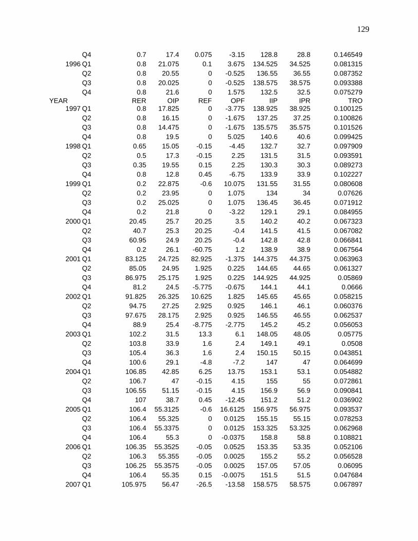
129
Q4 0.7 17.4 0.075 -3.15 128.8 28.8 0.146549
1996 Q1 0.8 21.075 0.1 3.675 134.525 34.525 0.081315
Q2 0.8 20.55 0 -0.525 136.55 36.55 0.087352
Q3 0.8 20.025 0 -0.525 138.575 38.575 0.093388
Q4 0.8 21.6 0 1.575 132.5 32.5 0.075279
YEAR 1997 Q1
RER 0.8
OIP 17.825
REF 0
OPF -3.775
IIP 138.925
IPR 38.925
TRO 0.100125
Q2 0.8 16.15 0 -1.675 137.25 37.25 0.100826
Q3 0.8 14.475 0 -1.675 135.575 35.575 0.101526
Q4 0.8 19.5 0 5.025 140.6 40.6 0.099425
1998 Q1 0.65 15.05 -0.15 -4.45 132.7 32.7 0.097909
Q2 0.5 17.3 -0.15 2.25 131.5 31.5 0.093591
Q3 0.35 19.55 0.15 2.25 130.3 30.3 0.089273
Q4 0.8 12.8 0.45 -6.75 133.9 33.9 0.102227
1999 Q1 0.2 22.875 -0.6 10.075 131.55 31.55 0.080608
Q2 0.2 23.95 0 1.075 134 34 0.07626
Q3 0.2 25.025 0 1.075 136.45 36.45 0.071912
Q4 0.2 21.8 0 -3.22 129.1 29.1 0.084955
2000 Q1 20.45 25.7 20.25 3.5 140.2 40.2 0.067323
Q2 40.7 25.3 20.25 -0.4 141.5 41.5 0.067082
Q3 60.95 24.9 20.25 -0.4 142.8 42.8 0.066841
Q4 0.2 26.1 -60.75 1.2 138.9 38.9 0.067564
2001 Q1 83.125 24.725 82.925 -1.375 144.375 44.375 0.063963
Q2 85.05 24.95 1.925 0.225 144.65 44.65 0.061327
Q3 86.975 25.175 1.925 0.225 144.925 44.925 0.05869
Q4 81.2 24.5 -5.775 -0.675 144.1 44.1 0.0666
2002 Q1 91.825 26.325 10.625 1.825 145.65 45.65 0.058215
Q2 94.75 27.25 2.925 0.925 146.1 46.1 0.060376
Q3 97.675 28.175 2.925 0.925 146.55 46.55 0.062537
Q4 88.9 25.4 -8.775 -2.775 145.2 45.2 0.056053
2003 Q1 102.2 31.5 13.3 6.1 148.05 48.05 0.05775
Q2 103.8 33.9 1.6 2.4 149.1 49.1 0.0508
Q3 105.4 36.3 1.6 2.4 150.15 50.15 0.043851
Q4 100.6 29.1 -4.8 -7.2 147 47 0.064699
2004 Q1 106.85 42.85 6.25 13.75 153.1 53.1 0.054882
Q2 106.7 47 -0.15 4.15 155 55 0.072861
Q3 106.55 51.15 -0.15 4.15 156.9 56.9 0.090841
Q4 107 38.7 0.45 -12.45 151.2 51.2 0.036902
2005 Q1 106.4 55.3125 -0.6 16.6125 156.975 56.975 0.093537
Q2 106.4 55.325 0 0.0125 155.15 55.15 0.078253
Q3 106.4 55.3375 0 0.0125 153.325 53.325 0.062968
Q4 106.4 55.3 0 -0.0375 158.8 58.8 0.108821
2006 Q1 106.35 55.3525 -0.05 0.0525 153.35 53.35 0.052106
Q2 106.3 55.355 -0.05 0.0025 155.2 55.2 0.056528
Q3 106.25 55.3575 -0.05 0.0025 157.05 57.05 0.06095
Q4 106.4 55.35 0.15 -0.0075 151.5 51.5 0.047684
2007 Q1 105.975 56.47 -26.5 -13.58 158.575 58.575 0.067897
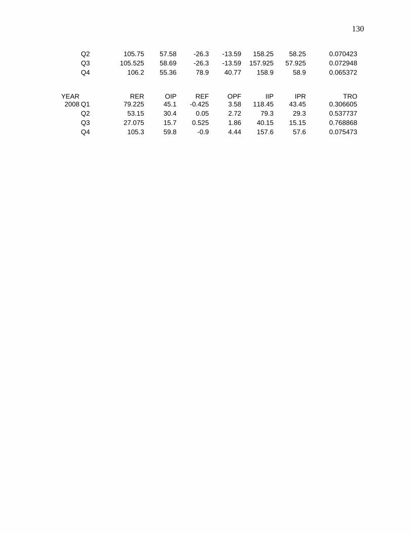
130
Q2 105.75 57.58 -26.3 -13.59 158.25 58.25 0.070423
Q3 105.525 58.69 -26.3 -13.59 157.925 57.925 0.072948
Q4 106.2 55.36 78.9 40.77 158.9 58.9 0.065372
YEAR 2008
Q1
RER 79.225
OIP 45.1
REF -0.425
OPF 3.58
IIP 118.45
IPR 43.45
TRO 0.306605
Q2 53.15 30.4 0.05 2.72 79.3 29.3 0.537737
Q3 27.075 15.7 0.525 1.86 40.15 15.15 0.768868
Q4 105.3 59.8 -0.9 4.44 157.6 57.6 0.075473
Recommended