Excess Smoothness of Consumption,
Consumption Insurance, and Correlated
Income Shocks
Dmytro Hryshko∗
University of Alberta
Abstract
In the literature, econometricians typically assume that household income is the sum ofa random walk permanent component and a transitory component, with uncorrelatedpermanent and transitory shocks. Using data on realized individual incomes and indi-vidual expectations of future incomes from the Survey of Italian Households’ Incomeand Wealth, I find that permanent and transitory shocks are negatively correlated.Relaxing the assumption of no correlation between the shocks, I explore the effectsof correlated income shocks on the estimated consumption insurance against perma-nent and transitory shocks, and consumption smoothness using a life-cycle model withself-insurance calibrated to U.S. data. Negatively correlated income shocks result intosmoother consumption, and upward-biased estimates of the insurance against transi-tory (and permanent when borrowing constraints are not tight) income shocks. Whilethe life-cycle model with negatively correlated shocks fits well the sensitivity of con-sumption to current income shocks observed in U.S. data, it falls short of explainingthe sensitivity of consumption to income shocks cumulated over a longer horizon.
Keywords: Buffer stock model of savings; Consumption dynamics; Life cycle; Incomeprocesses; Correlated shocks; Permanent-transitory decomposition.
JEL Classifications: C15, C61, D91, E21.
∗University of Alberta, Department of Economics, 8-14 HM Tory Building. Edmonton, Alberta, Canada,T6G 2H4. E-mail: [email protected]. Phone: 780-4922544. Fax: 780-4923300.
1 Introduction
Since Friedman (1957), household income is typically modeled as the sum of a permanent
random walk component and a short-lived transitory component, with no correlation between
transitory and permanent income shocks.
Models of household consumption over the life cycle that allow for self-insurance and
liquidity constraints predict that households insure against transitory shocks almost perfectly
but achieve limited insurance of permanent shocks. Using simulations of a buffer stock model
of savings Carroll (2009) finds, for a plausible set of parameters, that (simulated) households
are able to smooth only between 8 to 25 percent of permanent shocks to income. However,
Blundell, Pistaferri, and Preston (2008) and Attanasio and Pavoni (2011) recently showed,
using U.S. and U.K. data respectively, that households achieve substantial insurance against
permanent income shocks. Following the literature on consumption dynamics in macro data,
household consumption is said to be “excessively smooth.”1
In this paper, I examine excess smoothness of consumption in the standard life-cycle
model with self-insurance calibrated to US data, adding to the model a novel feature of
correlation between permanent and transitory shocks to household income.2, 3 I show that
the sensitivity of consumption growth to current income growth is smaller the more negative
is the correlation between the shocks. Negative correlation between the shocks, therefore,
may provide some scope for explanation of excess smoothness of consumption.
I calibrate life-cycle models with self-insurance, with the same value of the average wealth-
to-income ratio in the simulated economies, and the same amount of household income
risk measured by the variance of household income growth estimated using data from the
Panel Study of Income Dynamics (PSID). I also estimate consumption smoothness moments
1If income is non-stationary and income growth exhibits positive serial correlation—as supported byaggregate data—the Permanent Income Hypothesis (PIH) predicts that consumption should change by anamount greater than the value of the current income shock. Consequently, consumption growth should bemore volatile than income growth. Consumption growth in aggregate data, however, is much less volatilethan income growth. Therefore consumption growth is said to be “excessively smooth” relative to incomegrowth. See, e.g., Deaton (1992) and Ludvigson and Michaelides (2001) for a more recent account.
2Friedman (1963), in an attempt to clarify the controversial points in his book on the consumptionfunction, pointed out that the correlation between permanent and transitory shocks may be of any sign and,if present, should be allowed for in analysis of the consumption function.
3See also Browning and Ejrnæs (2013b) for a detailed analysis of the permanent-transitory decompositionof earnings when the shocks are correlated. Browning and Ejrnæs (2013a), p. 224, note that “Universallyin the earnings literature, it is assumed that the shocks . . . are uncorrelated; this is a difficult assumptionto maintain.”
1
using data from the Consumer Expenditure Survey (CEX) and PSID.4 In the model with
uncorrelated permanent and transitory income shocks, I confirm that household consumption
in the U.S. is excessively smooth, that is, the model predicts that households should be more
sensitive to income shocks than what is found in the data. While the model with negatively
correlated permanent and transitory income shocks fits well the reaction of consumption to
current income shocks, it still falls short of explaining the MPC out of shocks cumulated
over longer horizons; that is, consumption is still excessively smooth in the data. The key to
successful fitting of consumption sensitivity to current income shocks is that a negative (and
positive) permanent shock is partially smoothed, contemporaneously, by a transitory shock of
the opposite sign. However, because this smoothing is short-lived while the permanent shock
doesn’t die out, this mechanism is not enough to explain the sensitivity of consumption to the
shocks cumulated over a longer horizon—a certain degree of partial smoothing of permanent
shocks over longer spans is still needed to fit the consumption smoothness moments. Deaton
(1992), in a summary of the literature on consumption volatility in aggregate data, defines
excess smoothness as an insufficient responsiveness of consumption to the current income
shock. The model with negatively correlated shocks is, therefore, capable of explaining excess
smoothness in household data as defined in Deaton (1992) but the results in this paper
highlight that excess smoothness should be evaluated—in macro and household data—not
only against the adjustment of consumption to current income shocks, but also to the shocks
cumulated over longer horizons.
While evidence on the negative correlation between the shocks is indirect—via helping
fit the consumption smoothness moments in U.S. data better—one may opt out for direct
evidence if the data on income realizations and expectations are available.5 Unfortunately,
such data do not exist in US household surveys but are available from the Survey of Italian
Households’ Income and Wealth (SHIW), widely used in the literature on household choices
such as consumption and savings.6 Using data from the SHIW, I estimate permanent and
4Specifically, I measure consumption smoothness moments with the sensitivity of consumption to currentincome growth, and income growth cumulated over four years. The use of four-year growth rates allows me toexplore the reaction of consumption growth to income shocks cumulated over a longer horizon, when perma-nent shocks become relatively more important. More information on this choice is provided in footnotes 13and 25, and related discussion in the text.
5Note, however, that this is true of any indirect-inference type estimation (or calibration) that aims atrecovering parameters which are not directly observed, such as the time discount factor and the coefficientof relative risk aversion in Gourinchas and Parker (2002), or the variance of heterogeneous income profilesin Guvenen and Smith (2013).
6See, e.g., Guiso, Jappelli, and Pistaferri (2002), Jappelli and Pistaferri (2011), and Kaufmann andPistaferri (2009).
2

transitory shocks to individual incomes and find that they are negatively correlated, with
the correlation coefficient of about –0.50. There are a number of mechanisms that may lead
to correlation between the shocks. For example, job displacement often entails a period of
unemployment and a permanent loss in individual income.7 In such a case, a permanent
shock to household income due to job loss may be accompanied by its transitory and partial
smoothing via a payout of an unemployment insurance benefit, or a severance pay. Similarly,
a mild or moderate disability may entail a permanent loss in productivity and income, and
involve a sickness-leave transfer, which may result into a negative correlation between the
permanent and transitory shock. As another example, promotions may lead to a negative
correlation between permanent and transitory income shocks. Belzil and Bognanno (2008),
using earnings data for American executives in U.S. firms, find that promotions (followed
by positive permanent income raises) come together with bonus cuts (negative transitory
income shocks).8
Consumption smoothness observed in the data is intimately linked to the extent to which
households are able to insure against permanent and transitory shocks. Blundell, Pistaferri,
and Preston (2008) (BPP) proposed a methodology for measuring consumption insurance in
the data, while Kaplan and Violante (2010) focused on identification of consumption insur-
ance against uncorrelated permanent and transitory shocks within a life-cycle model with
self-insurance using that methodology. In addition to the findings in Kaplan and Violante
(2010), I show that the BPP-estimates of the insurance coefficients for transitory and perma-
nent shocks are upward-biased if the shocks are negatively correlated, and downward-biased
if the shocks are positively correlated. The bias for the estimated insurance of permanent
shocks is, however, likely to be small in the data.
The rest of the paper is structured as follows. In Section 2, I introduce the income
process, and discuss how correlated income shocks may affect the insurance coefficients for
transitory and permanent shocks, and consumption smoothness moments. In Section 3, I
provide direct evidence on the correlation between the shocks using Italian SHIW data. In
Section 4, I present the life-cycle model calibrated to U.S. data. In Section 5, I discuss results
from simulations of the model. Section 6 concludes.
7See Jacobson, LaLonde, and Sullivan (1993) and Kletzer (1998).8Browning and Ejrnæs (2013b) list some other potentially observable events that may result into a
negative or a positive correlation between the shocks.
3
2 The income process, correlated income shocks, and
excess smoothness of consumption
2.1 The income process
Let household i’s log idiosyncratic income at time t, yit, be composed of a persistent com-
ponent, pit, and a transitory component represented by an iid shock, ϵit:9
yit = pit + ϵit, ϵit ∼ iid(0, σ2ϵ ) (1)
pit = ρppit−1 + ξit, ξit ∼ iid(0, σ2ξ )
E[ξitϵit] = ρξ,ϵσξσϵ
E[ξit+jϵit] = 0, j = ±1,±2, . . .
ξit is the shock to the permanent/persistent component at time t, σ2ξ is the variance
of permanent/persistent shocks, ρp is the persistence of the shock ξit, σ2ϵ is the variance
of transitory shocks, and ρξ,ϵ is the contemporaneous correlation between permanent and
transitory shocks. In the literature, it is typically assumed that persistent and transitory
shocks are not correlated (ρξ,ϵ = 0), and the permanent component is a random walk (ρp =
1). In the discussion below, I relax the first assumption but continue assuming that the
permanent component is a random walk. In Section 5, I will present some results when ρp is
allowed to be less than one, in which case the shock ξit still impacts on household incomes
at times t+ 1 and further but with a decaying strength.
2.2 Identification of the income process using income data
Uncorrelated shocks If the shocks are uncorrelated, identification of the income pro-
cess (1) is straightforward using income data alone. The variance of permanent and transi-
tory shocks can be identified using the following respective data moments:
σ2ξ = E[∆yit
j=1∑j=−1
∆yit+j]
σ2ϵ = −E[∆yit∆yit+1].
9Idiosyncratic income is typically a measure of income net of observable variation due to age, schooling,geographical location, aggregate effects, etc.
4
Correlated shocks While the variance of permanent shocks in model (1) is uniquely iden-
tified if the shocks are correlated or not, the variance of transitory shocks, and the correlation
between the shocks are not separately identified using income data alone. In particular, the
variance of permanent shocks can still be identified using the moment E[∆yit
∑j=1j=−1 ∆yit+j
].
The moment −E[∆yit∆yit+1], used for identification of the variance of transitory shocks in
the case of uncorrelated shocks, will identify the sum of the variance of transitory shocks
and covariance between the permanent and transitory shocks—the moment therefore does
not uniquely identify the variance of transitory shocks but recovers a biased estimate of
the variance of transitory shocks if permanent and transitory shocks are contemporaneously
correlated; the bias equals ρξ,ϵσξσϵ, and its size clearly depends on the true variance of tran-
sitory shocks and the correlation. Similarly, it can be shown that relying on the moments
for log incomes in levels will not help in recovering the variance of transitory shocks ei-
ther when the shocks are correlated. Specifically, the moments (E[yityit+1]− E[yityit−1]) and
(E[yityit]− E[yityit+1]) have been used by Heathcote, Perri, and Violante (2010) to identify
the variance of permanent and transitory shocks, respectively. While the first moment re-
turns σ2ξ if the true income process is as described in (1), the second moment returns the
sum of the variance of transitory shocks and covariance between the shocks, σ2ϵ + ρξ,ϵσξσϵ.
The income process will be also under-identified if ρp is less than 1, and the shocks are
correlated. In that case, the model (1) will have an ARMA(1,1) representation—the autore-
gressive part will enable identification of the persistence ρp, while the moving average part,
having only two unique moments, will allow for identification of only two parameters among
the remaining three unknown parameters, σ2ξ , σ
2ϵ , and ρξ,ϵ. In sum, separate identification
of the variance of transitory shocks and correlation between the shocks is not possible by
merely adding the number of income moments—using income data alone, it’s only possible
to identify the sum of the variance of transitory shocks and covariance between the shocks
in case they are correlated.
2.3 Consumption insurance and smoothness, and identification of
the income process using income and consumption data
Uncorrelated shocks When households are not borrowing constrained, a life-cycle model
of consumption with CRRA utility results into the following (approximate) relationship
5

between household consumption and income shocks:10
∆cit = ϕitξit + ψitϵit + error,
where cit is household i’s idiosyncratic log consumption at age t.11 The coefficients ϕit
and ψit measure the strength with which household consumption reacts to the permanent
and transitory shock, respectively; ϕit and ψit are functions of household risk and time
preferences, the volatility of permanent and transitory shocks, persistence of the shocks, and
household age. Blundell, Pistaferri, and Preston (2008) estimate average values of ϕit and
ψit, ϕ and ψ respectively, using U.S. data on household disposable income and consumption,
and find that they vary with household wealth, and education. Kaplan and Violante (2010),
in a life-cycle model with self-insurance calibrated to U.S. data, compare the model-based
estimates of ϕ and ψ to the values estimated in Blundell, Pistaferri, and Preston (2008), and
examine how household insurance against permanent and transitory shocks varies with age,
and persistence of the shocks to the permanent component of income, among other things.
Using simulated data from a model of consumption choices, the (average values of) in-
surance against permanent and transitory shocks could be recovered from a regression
∆cit = ϕξit + ψϵit + error. (2)
Although permanent and transitory shocks are not observed in the data, the coefficients
ϕ and ψ can be estimated, as in Blundell, Pistaferri, and Preston (2008), with the following
data moments:
ϕBPP =E[∆cit
∑j=1j=−1∆yit+j
]E[∆yit
∑j=1j=−1 ∆yit+j
] (3)
ψBPP =E [∆cit∆yit+1]
E [∆yit∆yit+1]. (4)
Blundell, Pistaferri, and Preston (2008) estimate ϕ and ψ to be about 0.64 and 0.05,
respectively, for their whole sample (36% of permanent and 95% of transitory shocks are
found to be insured). A life-cycle model with self-insurance predicts, for reasonable parame-
terizations, that ϕ is above 0.64, and therefore the model falls short of explaining the amount
10See Blundell, Pistaferri, and Preston (2008) for details.11Household idiosyncratic log consumption is typically defined as the residual from a regression of log
consumption on observables such as age, schooling, family size, the number of kids, time dummies, etc.
6
of insurance against income shocks available in the data. That is, consumption in the data
is excessively smooth (relative to the predictions of a life-cycle model with self-insurance).
The shocks in equation (2) are normally not observed but they are part of idiosyncratic
household income growth, ∆yit.12 The (combined) effect of household income shocks on con-
sumption can be analyzed using observable information on (residual) growth in consumption
and income:
∆cit = β∆yit + error. (5)
Using equation (2), the estimated sensitivity of consumption to current income shocks
can be expressed as:
β =ϕσ2
ξ + ψσ2ϵ
σ2ξ + 2σ2
ϵ
. (6)
Any consumption model that fits β estimated from equation (5) should be also consistent
with consumption reaction to the shocks cumulated over longer horizons measured by the
coefficient βj from an OLS regression:
∆jcit = β0 + βj∆jyit + error, (7)
where ∆jzit ≡ zit − zit−j, and zit is log consumption or log income.
It can be shown that the sensitivity of cumulative consumption growth to cumulative
income growth over j periods is measured by
βj =jϕσ2
ξ + ψσ2ϵ
jσ2ξ + 2σ2
ϵ
. (8)
Longer differences in log income will be largely dominated by permanent shocks, and this
should be reflected in the long differences in log consumption.13 The estimated values of ϕ
and ψ, together with the estimated income process, could be used to predict the values of
βj’s. Since the (non-linear) moments βj are typically not targeted when recovering ϕ and ψ
in the data (to gain efficiency, the latter are normally recovered from a minimum-distance
12Point-identification of permanent and transitory shocks in equation (1) is possible, however, if one hasaccess to panel data with individual incomes and individual expectations of future incomes. I will return tothis issue in Section 3 below.
13This can be seen by rewriting equation (8) asjϕσ2
ξ
var(∆jyit)+
ψσ2ϵ
var(∆jyit). Clearly, the loading factor on the
contribution of the variance of permanent shocks to βj increases with the horizon j.
7
procedure matching the atocovariance function of income and consumption growth, and
cross-covariances of income and consumption growth rates), βj’s provide additional informa-
tion about consumption reaction to the shocks beyond that contained in the estimates of ϕ
and ψ, ϕBPP and ψBPP. For instance, using the point estimates of ϕBPP and ψBPP, and the
(average) variances of permanent and transitory shocks in Blundell, Pistaferri, and Preston
(2008), equation (8) implies the values of β1 and β4 of 0.18 and 0.60 respectively, while in their
data β1 and β4 are equal to 0.15 and 0.23, both with robust standard errors of about 0.02.
While the estimated values of insurance parameters in BPP fit well β1, they result in sub-
stantial overprediction of β4. Alternatively, one can use a structural model of consumption
and the data moments βj’s as auxiliary parameters in the indirect inference or method-of-
simulated-moments procedures to recover the degree of insurance against permanent and
transitory shocks, due to self-insurance (and other mechanisms), as is done, e.g., in Guvenen
and Smith (2013) and Hryshko (2010). In the indirect-inference approach of Guvenen and
Smith (2013), for instance, the data moments ϕBPP and ψBPP are not explicitly targeted but
fitting a structural model to the data moments such as βj’s will produce the model-implied
estimates of ϕBPP and ψBPP. As β1 and β4 are lower in the data than what is implied by the
BPP estimates of ϕ and ψ, it is not surprising that the indirect-inference approach, explic-
itly targeting the moments (similar to) βj’s but not the BPP moments themselves, typically
recovers a higher value of partial insurance of permanent shocks (total insurance, inclusive
of the insurance implied by borrowing and saving) than is found in BPP.14 In sum, both sets
of moments—ϕBPP and ψBPP, and βj’s—are potentially useful for evaluating consumption
smoothness in models with consumption and savings choices over the life cycle.
Correlated shocks When the shocks are correlated, the moments (3)–(4) no longer re-
cover the true values of ϕ and ψ from equation (2). While the coefficients ϕ and ψ estimated
using equation (2) (and observable permanent and transitory shocks from the model data)
will be the same if the shocks are correlated or not (since ϕ, e.g., measures the effect of
the permanent shock net of its correlation with the transitory shock), the correlation will
affect the estimated values of ϕBPP and ψBPP using the moments in equations (3)–(4). In
14Guvenen and Smith (2013), for a different parametrization of the income process, find that about 50%of income surprises are insured on top of borrowing and saving by consumers. Hryshko (2010) finds a similarnumber for the income process in equation (1).
8

particular, the estimated value of ϕBPP will equal
ϕBPP,corr =ϕσ2
ξ + ψρξ,ϵσξσϵ
σ2ξ
, (9)
while the bias in the estimated insurance of permanent shocks equals
(1− ϕBPP,corr)− (1− ϕ) = −ψρξ,ϵσϵσξ. (10)
The estimated insurance of permanent shocks will be biased upward (downward) if the
shocks are negatively (positively) correlated. Clearly, the bias depends on the correlation
of the shocks, and the size of the ratio of the variance of transitory shocks to the variance
of permanent shocks but will likely be small as the reaction of household consumption to
transitory shocks, ψ, is typically estimated to be close to zero.
The estimated value of ψBPP, in turn, will equal
ψBPP,corr =ψσ2
ϵ + ϕρξ,ϵσξσϵρξ,ϵσξσϵ + σ2
ϵ
, (11)
and the bias in the estimated insurance of transitory shocks will equal
(1− ψBPP,corr)− (1− ψ) = (ψ − ϕ)ρξ,ϵσξσϵ/(ρξ,ϵσξσϵ + σ2ϵ ). (12)
If ρξ,ϵ is positive, the bias is unambiguously negative, so that the insurance of transitory
shocks, 1 − ψBPP, estimated with equation (4) will be biased downward. When the shocks
are negatively correlated and∣∣∣ρξ,ϵ σξσϵ ∣∣∣ < 1, since ϕ > ψ, the estimated insurance of transitory
shocks will be biased upward.
Furthermore, if the shocks are correlated, equation (6) is modified to
β =ϕσ2
ξ + ψσ2ϵ + (ϕ+ ψ)ρξ,ϵσξσϵ
var∆yit. (13)
Since ψ is numerically low and the variance of permanent shocks is the same if the
shocks are correlated or not, β will be lower the more negative is the correlation between
the shocks. Correlation between the shocks, therefore, provides some scope for explanation
of excess smoothness in household consumption. Equation (13) highlights an important
point raised by Quah (1990) in the context of excess smoothness puzzle in the aggregate
data: holding constant the variance of income growth, the size of β will be dependent on
9
the relative importance of transitory and permanent components in income, or, in terms of
equation (13), the variances of permanent and transitory shocks.
Equation (13) shows that an empirical estimate of β from regression (5), together with
a structural model of consumption choices, will help identify the correlation between per-
manent and transitory shocks. The model will pin down ϕ and ψ, the income data will
allow for identification of σ2ξ , and the data estimates of the first-order autocovariance of
income growth and β will provide enough information to separately identify the variance of
transitory shocks, σ2ϵ , and the correlation between the shocks, ρξ,ϵ.
When the shocks are correlated, the sensitivity of cumulative consumption growth to
cumulative income growth over j periods is measured by
βj =jϕσ2
ξ + ψσ2ϵ + (ϕ+ jψ)ρξ,ϵσξσϵ
jσ2ξ + 2σ2
ϵ + 2ρξ,ϵσξσϵ. (14)
While β1 allows for exact identification of the correlation between the shocks, βj’s mea-
sured for j > 1 can be used as overidentifying restrictions for the model with correlated
shocks.
Summary To summarize, correlation between the shocks affects empirical estimates of
the insurance coefficients for permanent and transitory shocks, as well as the sensitivity of
consumption to current income growth and income growth cumulated over longer horizons.
Negatively correlated income shocks result into smoother consumption, so that allowing for
this previously neglected mechanism may potentially explain excess smoothness of consump-
tion. Although correlation between the shocks cannot be identified using income data alone,
it is feasible to identify it using information on consumption sensitivity to current income
growth and a model of life-cycle choices of consumption and savings. Section 5 explores
these issues in detail.
3 Direct evidence on the correlation of income shocks
The previous discussion relied on the assumption that permanent and transitory shocks are
not directly observable. Otherwise, correlation between the shocks could be straightforwardly
recovered from a series of permanent and transitory shocks.
In this section, I use data from the Survey of Italian Households’ Income and Wealth
(SHIW) to estimate permanent and transitory shocks to individual incomes. Pistaferri (2001)
10
first showed how to point-identify transitory and permanent shocks to incomes using data
on expected and realized income growth in SHIW data. In the 1995 and 1998 waves of the
SHIW, individuals were asked about expectations of their future net disposable incomes,
which enables estimation of one-year expected growth in net incomes between years 1995
and 1996, and 1998 and 1999.15
Estimation of correlation using data on subjective expectations of future incomes
Assume that log income, yit, is described by the model (1) with ρp = 1. The growth rate in
income between 1995 and 1998 can then be written as:
yi,98 − yi,95 = ξi,96 + ξi,97 + ξi,98 + ϵi,98 − ϵi,95. (15)
For each individual i, the transitory shock in 1995 and 1998 can be identified using the
following two moments:
ϵi,95 = −E[∆yi,96|Ωi,95] (16)
ϵi,98 = −E[∆yi,99|Ωi,98], (17)
where Ωi,t is information available to individual i at time t when expectation about net
income for period t+1 is revealed. Thus, the sum of permanent shocks in equation (15) can
be calculated as:
ξi,96 + ξi,97 + ξi,98 = yi,98 − yi,95 − E[∆yi,96|Ωi,95] + E[∆yi,99|Ωi,98]. (18)
Alternatively, the sum of permanent shocks can be also calculated using the information
on expected income levels:
ξi,96 + ξi,97 + ξi,98 = E[yi,99|Ωi,98]− E[yi,96|Ωi,95]. (19)
The correlation between the sum of permanent shocks and the transitory shock in 1998
equals:cov(ξi,96+ξi,97+ξi,98,ϵi,98)√
var(ξi,96+ξi,97+ξi,98)√
var(ϵi,98). Assuming the variances of permanent and transitory
shocks, and the covariance between permanent and transitory shocks are time-invariant, one
15Net disposable income is defined as the sum of net wages and salaries and fringe benefits, pensions andother transfers, and income from buildings (actual and imputed rents). For more details, see documentationat http://www.bancaditalia.it/statistiche/indcamp/bilfait/docum.
11
can calculate the correlation between permanent and transitory shocks as
corr(ξit, ϵit) =√3cov(ξit−2 + ξit−1 + ξit, ϵit)√
σ2ξt−2
+ σ2ξt−1
+ σ2ξtσϵt
. (20)
Using the estimates of the sum of permanent shocks in equations (18) or (19) and an
estimate of the transitory shock in equation (17), I will calculate the correlation between the
shocks relying on equation (20).
The details of sample selection and calculation of expected incomes and growth rates
are as follows. I used data for individuals of ages 25 to 65 who are not retired, not self-
employed or students. I dropped individuals with inconsistent records on gender, and year
of birth. In 1995 and 1998, individuals were asked about their maximum and minimum next-
year expected net disposable income; in addition, they were asked about the probability of
receiving less than the midpoint between the stated minimum and maximum. As in Guiso,
Jappelli, and Pistaferri (2002) and Kaufmann and Pistaferri (2009), I assumed that expected
income distributions are triangular, and calculated expected incomes and income growth
rates for 1996 and 1999. I dropped observations if an individual’s record on the probability
of the midpoint is either zero or one, and the minimum and maximum of the individual’s
expected income distribution are different from each other. I also dropped observations
if an individual’s minimum and maximum are the same (no expected fluctuations in the
next-period income) but the probability of receiving income below the midpoint is different
from zero. Part of expected incomes and growth rates can be due to life-cycle or aggregate
effects common to individuals observed at the same age in the same year. I removed those
effects from expected incomes, expected and observed income growth rates by regressing
the first measure on a third-order polynomial in age and year dummies, and the latter
two measures on a quadratic polynomial in age and year dummies. The resulting sample
contains 367 individuals, with the majority represented by males, married individuals, and
individuals with a high school diploma or more education—see Table 1 for some sample
statistics. For this sample, the correlation between permanent and transitory shocks is about
–0.47 with a bootstrapped standard error of 0.11.16 Standard deviations of permanent and
transitory shocks agree with the estimates of Kaufmann and Pistaferri (2009) using the same
16Using equations (18) or (19) for estimation of (the sum of) permanent shocks delivers virtually identicalestimates of the correlation between permanent and transitory shocks. The correlation between the estimatesof permanent shocks using (18) or (19) is 0.99.
12

waves of SHIW data.17 The sample containing only heads is limited to 201 individuals; for
that sample, the correlation between the shocks is estimated at –0.52 with a bootstrapped
standard error of 0.14.
Robustness to serial correlation In the previous discussion, I assumed that the transi-
tory process is an iid shock. If the transitory component is instead a moving average process
of order 1, ϵit + θϵit−1, one needs E[∆yit+2|Ωit] to identify the transitory shock at t.18 In
the absence of such information (as is the case for Italian data), −E[∆yit+1|Ωit] identifies
(1 − θ)ϵit + θϵit−1. It follows that equation (17) would identify (1 − θ)ϵi,98 + θϵi,97, while
equation (18) would identify ξi,96 + ξi,97 + ξi,98 + θϵi,98 − θϵi,95. In this case, the numerator of
equation (20) would measure (1 − θ)cov(ξi,98ϵi,98) + (1 − θ)θσ2ϵ98. Since θ is normally found
to be positive and less than 1 in household data, the estimated correlation in equation (20)
would be biased towards zero if the true covariance between permanent and transitory shocks
is negative. Notice, however, that Jappelli and Pistaferri (2011), using the same dataset,
have found that income growth is not correlated with income growth two years from now
and on, which is consistent with the income process composed of a random walk and an iid
transitory shock. Jappelli and Pistaferri (2006) and Kaufmann and Pistaferri (2009) reach
the same conclusion.19
One could also use expected income growth between 1996 and 1995 to test for serial
correlation in the transitory component. If the true process is a random walk plus a mov-
ing average process of order 1, the covariance between E[yi,99|Ωi,98] − E[yi,96|Ωi,95], and
−E[∆yi,96|Ωi,95] will equal −θ(1−θ)σ2ϵ95, and will be negative if 0 < θ < 1, which is a typical
case in the literature. If the transitory component is an iid shock, as is assumed above, the
17Note that the value of the standard deviation of permanent shocks reported in Table 1 reflects thestandard deviation of the sum of permanent shocks between years 1998 and 1995, while Kaufmann andPistaferri (2009) report on the annual variance of permanent shocks.
18The income process composed of a random-walk permanent component and an MA(1) transitory com-ponent is considered, e.g., in Meghir and Pistaferri (2004).
19In the datasets where the transitory component contains a moving average process, i.e. when θ > 0,equation (20) no longer identifies correlation between the shocks but the moments (17) and (18) (right-hand-sides of the equations) can be used to bound the correlation given some plausible values of θ and thevariance of permanent shocks (which can in principle be uniquely identified without relying on the dataon expectations). In particular, for a given value of θ, the variance of transitory shocks will be uniquelyidentified using the data moment (17). One can further use the moment (18) to identify the covariancebetween the shocks; to pin down the correlation between the shocks, one would need a value for the varianceof permanent shocks. For the sample of all individuals, assuming that θ = 0.10 (the estimated value in BPPfor US data), correlation between the shocks equals about –0.40 (–0.20) when the variance of permanentshocks is half (twice) the variance of transitory shocks, while assuming that θ = 0.30 (in the upper range ofestimated values in Meghir and Pistaferri (2004) for US data), correlation between the shocks is about –0.70(–0.35) when the variance of permanent shocks is half (twice) the variance of transitory shocks.
13
covariance will equal zero. For the whole sample, an estimate of the covariance is 0.008 with
a robust standard error of 0.007, while for the sample comprised of heads only, an estimate
of the covariance is 0.01 with a robust standard error of 0.01—in both samples the data do
not appear to favor the hypothesis of a serially correlated transitory component.
Robustness to idiosyncratic trends In the literature, another popular alternative to the
permanent-transitory decomposition of household incomes is an income process that com-
prises an AR(1) persistent component, household heterogeneity in income profiles (growth
rates), and an iid transitory component—see, e.g., Guvenen (2009) who labels this income
process HIP. In this case, individual i with t years of labor market experience will have in-
come yit = βit+pit+ϵit, where pit = ρppit−1+ξit as in equation (1) but ρp is not restricted to
one, and βi is an individual-specific growth rate that averages out to zero in the population
and has variance σ2β. Note that the estimated covariance between E[yi,99|Ωi,98]−E[yi,96|Ωi,95]
and −E[∆yi,99|Ωi,98], used for identification of the correlation between the shocks above, will
not help differentiating between the income process (1) with ρp = 1 and correlated income
shocks and the income process with heterogeneous trends as both income processes may
predict a negative correlation.20 Under the income process with heterogeneous trends, how-
ever, the covariance between E[yi,99|Ωi,98]−E[yi,96|Ωi,95] and −E[∆yi,96|Ωi,95] will be negative
and equal to −ρp(1− ρp)2(ρ2p + ρp + 1)var(pi,95)− 3σ2
β.21 As this covariance is estimated to
be positive but insignificantly different from zero in the data, one may conclude that the
data are not supportive of the income process with heterogeneous trends and a moderately
persistent AR(1) component.
Summary Summarizing, there is evidence that permanent and transitory shocks to Italian
net disposable incomes are negatively correlated. Admittedly, this evidence is based on
small samples and more research is needed on larger samples for more conclusive evidence.
However, even these small samples are informative and favor the income process (1) with
20In particular, if the true income process is HIP, the covariance will equal ρ4p(1 − ρp)(ρ3p − 1)var(p95) +
(1− ρp)ρ5pσ
2ξ96
+(1− ρp)ρ3pσ
2ξ97
+(1− ρp)ρpσ2ξ98
− 3σ2β . Under the assumption that the variance of persistent
shocks is not changing over time, the smallest value of the term not involving the growth-rate heterogeneity(if the variance of persistent shocks is not zero) equals ρp(1−ρp)(1+ρp)−1(1+ρp+ρ
2p)σ
2ξ . Since the term is
positive, the smallest value of σ2β (when the variance of persistent shocks approaches zero) equals 0.028/3, or
0.009, where 0.028 is the negative of the estimated covariance in the data. Note also that the estimated valueof the covariance is not consistent with an income process that contains just an AR(1) persistent componentand an iid transitory component, as in this case the predicted covariance is positive while it is negative inthe data.
21The covariance equals zero if the true income process is (1) with ρp = 1 and correlated (or uncorrelated)permanent and transitory shocks as can be verified by setting ρp to 1 and σ2
β to zero in the expression.
14
contemporaneously correlated income shocks, and enable to rule out some alternative income
processes such as HIP, or an income process with serially correlated transitory shocks.
4 The model
In this section, I set up a model of household consumption choices over the life cycle, and
evaluate the quantitative importance of the correlation between permanent and transitory
shocks for consumption smoothness and consumption insurance.
I assume that households value consumption, supply labor inelastically, face income un-
certainty over the working part of the life cycle, and are subject to liquidity constraints.
Households start their working life at age 26, retire at age R = 65, face age-dependent
mortality risk until age T = 90 when they die with certainty. Household i’s problem is:
maxCitTt=0
Ei,26
T∑t=26
(1
1 + θ
)t−26
stU(Cit), (21)
subject to the budget constraint,
wit+1 = (1 + r)(wit + Yit − Cit), (22)
and the liquidity constraint:
wit ≥ wt, for t = 26, . . . , T. (23)
Cash-on-hand available to household i at age t, Xit = wit + Yit, consists of labor income
realized at t, Yit, and household wealth at age t, wit; r is a net interest rate on a risk-free asset
held between ages t and t + 1. θ is the common time discount rate, st is the unconditional
probability of surviving up to age t, Cit is household i’s consumption at age t, and Ei,26
denotes household i’s expectation about future resources based on the information available
at age 26. I assume that utility is CRRA, U(Cit) =C1−ρ
it
1−ρ , where ρ is the coefficient of
relative risk aversion. Households are subject to liquidity constraints so that their wealth is
constrained to be above wt—equation (23).
15
Calibration
Demographics I assume that households start their life cycle at age 26, retire at age
65, and die with certainty at age 90. Before retirement, the unconditional probability of
survival is set to 1; after the retirement, households face an age-dependent risk of dying.
The conditional probabilities of surviving up to age t provided the household is alive at age
t − 1 for all R < t ≤ T − 1 are taken from Table A.1 in Hubbard, Skinner, and Zeldes
(1994).22
Preferences, and the real interest rate I set the gross real interest rate to 1.03, and
the coefficient of relative risk aversion to 2.23 For comparability with Kaplan and Violante
(2010), I calibrate the time discount factor to match an aggregate wealth-to-income ratio of
2.5.
The income process I use the income process outlined in equation (1). I will consider the
permanent-transitory decomposition, with and without correlation between the shocks, but
will also model the permanent component as an autoregressive process. The age-dependent
deterministic growth rate in household disposable income is estimated using CEX data. I
decompose household disposable log income into cohort, time, and age effects, controlling
for the effect of family size. As is well known, age, cohort, and time effects are not separately
identified. To identify the age effects, I follow Deaton (1997) and restrict the time dummies
to be orthogonal to a time trend and to add up to zero. I use the age effects from such a
regression to construct the profile of deterministic growth in household disposable income.
Retirement After retirement, household income is assumed to be proportional to the
permanent component of income received at age R, Yit = κPiR for ages t = R + 1, . . . , T ,
where κ is the replacement rate.24 The replacement rate κ is set to 0.60. This value is similar
to an estimate of the replacement rate for U.S. high school graduates in Cocco, Gomes, and
Maenhout (2005).
22This is the mortality data on U.S. women for 1982.23In a general equilibrium setting, household desire to smooth consumption and the demand for precau-
tionary savings will affect the equilibrium interest rate and household ability to insure against permanentand transitory shocks (e.g., through the effect of interest rates on natural borrowing limits). While sucheffects are worth keeping in mind, they are not a subject of this paper.
24In the experiments outlined below, when the permanent component of income follows an autoregressiveprocess, income at retirement is assumed to be proportional to the value of the persistent component in thelast working period.
16

Initial wealth I assume that households start their working life with zero assets but will
also allow for a distribution of initial wealth levels estimated from PSID data in a robustness
experiment.
Borrowing limits I will consider two types of borrowing constraints, zero and natural
borrowing constraints. When households are subject to zero borrowing constraints, wealth
cannot be negative, that is wt = 0 for all ages t. Under the natural borrowing constraints,
households are allowed to borrow up to the age-dependent limit, equal to the largest amount
of credit they can repay in case they receive the lowest possible income realization in every
period.
Smoothness of consumption, insurance, and income moments I obtain consump-
tion information from two data sources, the CEX and the PSID. The CEX contains detailed
information on total expenditures and its components, and the demographics for representa-
tive cross sections of the US population. I use extracts from the 1980–2003 waves of the CEX
available at the National Bureau of Economic Research (NBER) webpage. Unlike the CEX,
the PSID provides panel data yet limits its coverage of consumer expenditures to food at
home and away from home. Since I am interested in the link between changes of household
disposable income and total household consumption, I impute the total consumption to the
sample PSID households using information on household food consumption in the PSID and
the CEX, and matched demographics from the CEX and the PSID. PSID data are taken
from the 1981–1997, 1999, 2001, and 2003 waves. I follow the methodology of Blundell,
Pistaferri, and Preston (2008) to impute total consumption to the PSID households. The
full details on sample selection of CEX and PSID households are provided in Appendix A.
Briefly, from the PSID, I choose married couples headed by males of ages 26–70 born be-
tween 1912 and 1978, with no changes in family composition (no changes at all or changes
in family members other than the head and wife). I drop income outliers, observations with
missing or zero records on food at home and, for each household, keep the longest period
with consecutive information on household disposable income and no missing demographics.
From the CEX, I choose households who are complete income and expenditure reporters,
with heads who belong to the same age groups and cohorts as in the PSID sample.
In the PSID, federal income taxes are recorded until 1991. To have a consistent measure
of federal income taxes for the data that extend beyond 1991, one needs to impute them
to the PSID households. I use the TAXSIM tool at the NBER to calculate federal income
17
taxes and social security withholdings for the head and wife and all other family members
if present.
I utilize data from the 1981–1997 surveys of the PSID to impute total household con-
sumption. For different model parameterizations below, I will tabulate the moments relating
to the extent of smoothness of consumption with respect to income changes measured by
βj’s; the true insurance coefficients, (1− ϕ) and (1− ψ), and the insurance coefficients esti-
mated using BPP moments, (1− ϕBPP) and (1− ψBPP); the variance of idiosyncratic income
growth, and the persistence of household disposable income. The consumption smoothness
is measured by the coefficients βj, j = 1 or 4, from the following panel regressions estimated
by OLS:
∆jcit = β0 + βj∆jyit + γ′xit + ϵit, (24)
where zit ≡ logZit− 1Nt
∑Nt
i=1 logZit for any variable z in the regression, Nt is the number of
observations in the regression sample at time t, ∆jzit ≡ zit − zit−j, and xit is a vector that
comprises a quadratic polynomial in the head’s age, and family size. I take out the time-
specific averages from the variables to remove the aggregate effects in the data. My focus
is on β1 and β4 and the model-implied values of the coefficients. The moment β1 is chosen
as it’s informative about the correlation between permanent and transitory shocks, while
the moment β4 is chosen as it weighs more the information on the importance of permanent
shocks in shaping the response of consumption to the shocks cumulated over a longer time
span.25
The estimated value of β1 is 0.12 with a standard error of 0.03, suggesting that about 12
percent of the shocks to current income are translated into consumption. This can be due
to the presence of a large transitory component in income, measurement error in income,
or different insurance mechanisms available to households for smoothing out fluctuations in
disposable income. The estimated value of β4 is 0.23 with a standard error of 0.03.
I measure mean reversion in household income estimating the coefficient α from the
following regression:
∆yit = α0 + α∆yit−1 + γ′xit + ϵit, (25)
where yit is log disposable household income at t, and xit is a vector that includes a quadratic
25I have chosen to focus on β1 and β4 for expositional clarity only; adding β2, β3, etc. into the discussionwill not bring any extra insights.
18
polynomial in the head’s age and dummies for the head’s high school graduation and college
completion. As in the previous regressions, I take out the time-specific means from each
variable prior to running the regression. The estimated value of α is –0.30 with a standard
error of 0.01.
The size of income risk over the life cycle is calculated as the variance of idiosyncratic
income growth. For its estimation, I first run cross-sectional regressions of the difference in
household log disposable income on a quadratic polynomial in the head’s age and dummies
for high school and college using data from the 1981–1997 surveys, when household income
was continuously recorded each year. I limit the regression sample to the households with
heads of ages 26–65. The unconditional variance of the residuals from those regressions
provides an estimate of the proportional risk to household disposable income over the life
cycle. The estimated variance is 0.048, and its standard error is 0.002. In all my calibrations,
I set the income process parameters such that the variance of household income growth rates
equals to its data value. In addition, I set the variance of permanent shocks to 0.01—this
is the choice of Kaplan and Violante (2010) which enables matching the rise in the variance
of incomes over the life cycle in the U.S.; below, I will elaborate on the consequences of this
choice for matching the income moments. The data moments are listed in Table 2. The
model is solved using the method of endogenous grid points of Carroll (2006).
5 Results
Table 3 shows the results when the income process contains a permanent random-walk
component and households are not allowed to borrow. The outline of this table and the
tables to follow is the following.
• Columns (1) and (3) present the amount of insurance against permanent and transitory
shocks estimated using equation (2). Specifically, I tabulate (1− ϕ) and (1− ψ) using
information on household consumption, and permanent and transitory shocks from the
model data. I label them “Model true” estimates in the tables.
• Columns (2) and (4) tabulate the insurance coefficients estimated using equations (3)
and (4), (1− ϕBPP) and (1− ψBPP), respectively. They are labeled “Model BPP” esti-
mates in the tables. Those estimates are based on the data on household consumption
and income from the model, and the moments suggested by Blundell, Pistaferri, and
19

Preston (2008)—unlike the estimates in columns (1) and (3), they do not rely on the
knowledge of permanent and transitory shocks to each household’s income at each age.
• Column (5) reports the time discount factor needed to match an aggregate wealth-to-
income ratio of 2.5.
• Columns (6) and (7) report on the reaction of consumption changes to current in-
come shocks and income shocks cumulated over the 4-year horizon estimated using
equation (7).
• Column (8) shows the persistence of income shocks estimated with equation (25).
Zero borrowing constraints In the first row, I assume that the shocks are not correlated,
and one standard deviation of permanent shocks equals 0.10, as in Kaplan and Violante
(2010). One standard deviation of transitory shocks is set to 0.14—to fit the variance of
household income growth of 0.048 estimated in the data. This results into a faster mean
reversion of household incomes than in the data: α is estimated at –0.40 in column (8) relative
to the data value of –0.30. To fix this, one would need a higher value for the variance of
permanent shocks and a lower value for the variance of transitory shocks but I chose to
keep the standard deviation of permanent shocks at 0.10 for comparability with Kaplan and
Violante (2010).26 A lower value for the variance of permanent shocks would be obtained if
one was fitting the income process matching the moments α, the variance of income growth
rates, and the rise in the variance of incomes over the life cycle putting relatively larger
weights on the latter two moments.
I find that households insure 13% of permanent shocks, and 88% of transitory shocks in
the no-borrowing environment—columns (1) and (3).27 Similarly to Kaplan and Violante
(2010), insurance of permanent shocks calculated in accordance with (3)—as in Blundell,
Pistaferri, and Preston (2008)—is biased downward. As highlighted in Kaplan and Violante
26 If, instead, I chose to fit the persistence of shocks of –0.30, observed in the data, and the variance ofincome growth of 0.048, the standard deviation of permanent shocks would equal 0.14 and the standarddeviation of transitory shocks would equal 0.12.
27A higher value for the insurance of permanent shocks in Kaplan and Violante (2010) is likely due todifferences in modeling of pension benefits. Since pension benefits are tied to the average career earningsin Kaplan and Violante (2010), permanent shocks in the end of life cycle produce a little effect on thepermanent income, and, as a result, a little effect on household consumption in their setup. This impliesa high value of consumption insurance in the end of working career. If pensions are tied to the permanentcomponent of income in the end of working career, as is assumed here, permanent shocks will have a largereffect on household permanent income, and household consumption will react more to permanent shocks inthe end of working career, implying a relatively lower value of insurance against permanent shocks.
20

(2010), the bias arises due to the failure of orthogonality between household consumption
growth at t, ∆cit, and the transitory shock at t− 2, ϵit−2, when households are not allowed
to borrow. The bias is lower in magnitude than in Kaplan and Violante (2010) but this
could be explained by their choice of a relatively higher ratio of the standard deviation of
transitory shocks to the standard deviation of permanent shocks.28
Insurance of transitory shocks calculated as in Blundell, Pistaferri, and Preston (2008)
is an unbiased estimate of the true insurance in the model. See the left panel in Figure 1
for the age profile of insurance against permanent and transitory shocks when households
are not allowed to borrow. Clearly, the bias in the BPP-estimate of permanent insurance
arises due to household inability to borrow at early ages in the life cycle. The sensitivity of
consumption at one and four-year horizons, β1 and β4, is about twice as large in the model
as in the data—the model predicts that consumption under-reacts to income shocks in the
data, that is, household consumption is excessively smooth.
In the second row, I assume that the correlation between permanent and transitory shocks
equals –0.40, which is close to the values estimated in Section 3 using Italian data.29 As
I keep the variance of household income growth constant across different experiments at
0.048, this results into a higher variability of transitory shocks—a one standard deviation in
transitory shocks is 0.16 vs. 0.14 in the first row. The extent of insurance against transitory
shocks estimated using the moment (4) is substantially biased upward. This is in line with
the prediction in Section 2. Notice that while the true insurance against permanent and
transitory shocks is unchanged, the model-based estimate of consumption smoothness β1—
due to a negative correlation between the shocks—is close to the data counterpart of 0.12.
The model, however, still overpredicts the extent of consumption reaction to the shocks
cumulated over the four-year horizon. Although the short-run smoothness of consumption
is well explained by partial smoothing of the permanent shock due to negative correlation
28The ratio equals 1.4 in the first row of Table 3, while it is about 60% higher, and equals 2.24 in Kaplan andViolante (2010). It can be shown that the bias in the estimated insurance of permanent shocks, (1− ϕBPP)−(1 − ϕ), equals
corr(∆cit,ϵit−2)σ∆ctσϵ
σ2ξ
and is negative as the model-implied correlation between consumption
growth at age t and the transitory shock at age t− 2 is negative. That the bias is very sensitive to the ratioof the variance of transitory shocks to the variance of permanent shocks can be also seen in the sensitivityexperiments of Table 3 in Kaplan and Violante (2010).
29When the shocks are correlated, the transitory shock can be expressed as ϵ = κξ + µ, where κ = ρξ,ϵσϵ
σξ
and σ2µ = (1− ρ2ξ,ϵ)σ
2ϵ . Clearly, information on the permanent and transitory shock could be reduced to one
state variable if the shocks are perfectly correlated. However, if the shocks are imperfectly correlated, thestate vector should include information on ξ and µ, which are mutually orthogonal—the main point, though,is that household decisions will take into account partial smoothing (or amplification in the case of positivecorrelation) of the permanent shock which is reflected in the correlation between ϵ and ξ.
21

between the shocks, this mechanism is not enough for explaining a longer-term smoothness of
consumption—a certain degree of partial smoothing of permanent shocks over longer spans
is still needed to match β4.
In the third row, I assume the correlation between the shocks is positive, and equals
0.40. The BPP-estimate of the insurance against transitory shocks is substantially biased
downward, as predicted in Section 2. Although the true insurance against permanent and
transitory shocks is virtually unchanged, a positive correlation between the shocks is reflected
in larger values of consumption sensitivity to the current income shocks and shocks cumulated
over the four-year horizon.
While assuming a negative correlation between the shocks is in line with the findings
in Section 3, it is possible that the distributions of permanent and transitory shocks are
independent but some market mechanism or an endogenous reaction to the shocks within a
household may result into household income changes and consumption allocations resembling
the case of income shocks correlated period-by-period. For example, a head’s layoff may
entail a permanent negative effect on his income (e.g., via loss of a firm-specific human
capital) but may be accompanied by a payout of unemployment insurance benefits or a
severance pay which may work as a positive transitory shock. A similar mechanism for the
negative correlation between permanent and transitory shocks is suggested in Browning and
Ejrnæs (2013b). Such event is rare but there are other observable rare events that may
potentially result into a positive or a negative correlation between permanent and transitory
shocks such as health shocks, promotions, or job mobility. As it is infeasible to properly
model a myriad of such events, the (likelihood of) occurrence of all of which could affect
household consumption decisions, I will focus below on a “representative” rare event that
results into an opposite movement of a permanent and transitory shock on its incidence. This
is inspired by two key findings above: first, the permanent and transitory shock are shown
to be, on average, negatively correlated in Italian data, and, second, the case of negatively
correlated shocks is plausible from the standpoint of consumption data as it may help better
fit the sensitivity of consumption to income growth, and help explain excess smoothness of
consumption.
Below, I will model this rare event in a stylized way. I first assume that the “rare shock”
results into a permanent loss of d = 20% of household income, and is accompanied by a
transitory increase in income of 10% so that, at the time of the shock, household income
falls by 10%. The transitory increase in income is meant to represent an unemployment
insurance benefit that is exhausted within a year, a severance pay, or a sickness-leave pay in
22

case of a mild/moderate disability.30 I assume that the “rare shock” happens with a pd = 5%
probability and is an iid event.31
To match the increase in the variance over the life cycle in the previous calibrations,
I adjust the standard deviation of permanent shocks downward to 0.09.32 The implied
correlation between the permanent shock (which equals the sum of the permanent shock
and permanent income loss due to the rare shock) and the transitory shock (equals the sum
of the transitory shock and transitory payment at the time of the rare shock) is −0.08.
The results of this experiment are presented in the fourth row of Table 3. Similarly to the
calibration in the second row, there’s an upward bias of the BPP-estimate of the insurance
against transitory shocks. Since the implied correlation is above –0.40, the bias is numerically
smaller. See Panel A of Figure 2 for the age profile of insurance against permanent and
transitory shocks when households are not allowed to borrow. As in the environment of no
correlation between the shocks, there’s a downward bias in the BPP-estimates of insurance
against permanent shocks at early stages of the life cycle; an upward bias in the estimated
insurance of transitory shocks is, however, not limited to the stage of the life cycle.
In the fifth row, I experiment with a larger “rare shock” that results into a 40% permanent
loss of income. A one standard deviation of the permanent shock is set to 0.04 to match the
increase of the life cycle variance in the previous calibrations. This results into the correlation
between permanent and transitory shocks of about –0.30. Since the implied correlation is
closer in magnitude to the correlation in the second row, the bias in the BPP-estimate of
the insurance against transitory shocks as well as the consumption smoothness moments
are similar to the corresponding values in the second row. The corresponding age profiles
of insurance against permanent and transitory shocks are shown in Figure 2, Panel B. The
pattern is qualitatively similar to that in the low rare-shock case, and quantitatively similar
to the case when the shocks are correlated period by period (Figure 2, Panel C).
30See, e.g., Jacobson, LaLonde, and Sullivan (1993) for some evidence on displaced workers’ earningslosses. Kletzer (1998) presents evidence that job displacement is often followed by a spell of unemployment.See Engen and Gruber (2001) for evidence that unemployment insurance benefits are temporary in naturein the U.S.
31The numbers for the probability of rare shock and permanent income loss due to the shock are similarto the corresponding numbers in Krebs (2007) for job displacement. They are based on Jacobson, LaLonde,and Sullivan (1993) who, however, showed that short-term earnings losses due to job displacement are higherthan long-term losses. Nevertheless, the magnitude and the pattern of earnings losses in the short and longterms are consistent with the effect of disability on head’s earnings in PSID data—see Stephens (2001),Figure 2.
32As in Krebs (2007), I assume that with probability (1− pd) household income is permanently raised bya small value dpd/(1− pd). This is done to ensure that income shocks are mean-zero, and is inessential forthe results to follow.
23

Natural borrowing constraints Table 4 contains the results when households are con-
strained by natural borrowing limits. The discrepancy between the true and BPP-estimates
of insurance against permanent shocks is nearly eliminated, while the insurance of transi-
tory shocks is higher, at 95%—see the first row, and the right panel of Figure 1 for the age
profiles of insurance coefficients for permanent and transitory shocks. For the experiments
in the second, fourth, and fifth rows of the table, the BPP-estimate of the insurance against
transitory shocks is upward-biased, with the highest bias for the cases with a negative cor-
relation between the shocks of –0.40 and a large rare shock; see also Panels A, B and C in
Figure 3 for the age profiles of insurance coefficients for permanent and transitory shocks for
the cases of low, large rare shocks, and the shocks correlated period-by-period, respectively.
The estimated sensitivity of consumption to the shocks cumulated over one and four-year
horizons is smaller when natural borrowing constraints are allowed for. When the shocks
are negatively correlated, β1 is slightly lower than its data counterpart; the size of β4, how-
ever, is still higher in the model than in the data—consumption is still excessively smooth.
As Euler equations are likely to hold at equality when borrowing constraints are not tight,
the biases in the insurance coefficients estimated with equations (10) and (12) should ap-
proximate well the biases seen in the model data. For the parameters in the second row of
Table 4, equation (10) predicts a bias in the estimated permanent insurance of about 0.03,
while equation (12) predicts a bias in the transitory insurance of about 0.28. These numbers
compare well with the numbers in Table 4. For the case of positive correlation in the third
row, the permanent insurance should be underestimated by about 0.02, while the transitory
insurance should be underestimated by about 0.21 in accordance with equations (10) and
(12)—the numbers are in accord with the numbers in the table.
Summary The results for rare shocks and the shocks correlated period-by-period are quan-
titatively similar when an implied correlation between the shocks is similar. Clearly, what
matters for this result is that a negative (and positive, in the case of period-by-period cor-
relation) permanent shock is partially smoothed by a transitory shock of the opposite sign.
This allows to better fit the sensitivity of consumption to current income shocks (the moment
β1). However, because the smoothing is short-lived while the permanent shock doesn’t die
out, this mechanism is not enough to explain the sensitivity of consumption to the shocks
cumulated over a longer horizon (the moment β4)—a certain degree of partial smoothing of
permanent shocks over longer spans is still needed to fit the consumption moments. Below,
I will focus on the case of period-by-period correlated shocks with correlation of –0.40 as
24

this is the value close to my estimate from SHIW data, and is also the value which provides
a better fit to the consumption smoothness moments β1 and β4 in U.S. data, as opposed to
the case of uncorrelated shocks.
Sensitivity analysis In Table 5, I conduct a number of sensitivity experiments. The table
is split into two panels: the top panel contains the results for zero borrowing constraints,
while the bottom panel contains the results for natural borrowing constraints.
In the first two rows of both panels, I allow for rare shocks, low and large respectively, but
I assume away partial compensation of the shock in the form of a positive transitory shock.
This eliminates the bias in the BPP-estimates of the insurance against transitory shocks, in
agreement with the results in Section 2. While the BPP-estimate of the insurance against
permanent shocks is downward-biased when households are not allowed to borrow, the bias
gets eliminated when households are allowed to borrow up to the natural limit. Interestingly,
the estimates of β1 and β4 are similar when the rare shock is low or large, despite a much
lower variance of permanent shocks arriving each year in the case when the rare shock is
large.
The third row in each panel of Table 5 shows the results when the correlation between
the shocks is allowed for but the coefficient of relative risk aversion is set to a higher value
of 10. Relative to the results in the second rows of Tables 3–4, the insurance coefficients for
permanent shocks are higher; interestingly, the sensitivity of consumption to current income
shocks and shocks cumulated over 4 years—measured by β1 and β4—barely changes despite
a much higher value for the coefficient of relative risk aversion. Due to negative correlation,
the BPP-estimates of insurance against transitory and permanent shocks are upward-biased
even for the case of high individual aversion to risk.
The fourth to sixth rows of the table show the results when households differ in wealth
at the start of their working career.33 Overall, the results are very similar to the case when
every household starts its working career with zero wealth. The fifth and sixth rows in
each panel partition the sample into households who started the life cycle with low and
high wealth, respectively. High-wealth (low-wealth) households are those whose wealth at
age 26 is above (below) the 75th (25th) percentile of the wealth distribution at age 26.
Wealthier households have a larger insurance of permanent shocks under zero and natural
borrowing constraints, and a larger insurance of transitory shocks when borrowing is not
allowed. Under zero borrowing constraints, there is a more pronounced difference between
33I use PSID data to calibrate the distribution of initial wealth with household wealth data at ages 26–30.
25

high- and low-wealth households in consumption sensitivity to the income shocks measured
by the coefficients β1 and β4.
Autoregressive “permanent” component In Table 6, I explore the possibility that the
permanent component is an autoregressive process with a finite persistence of the shock. The
table is split into two panels with the results for zero and natural borrowing constraints. The
first two rows in each panel contain the results when the persistence of an AR(1) permanent
component, ρp, equals 0.99 and the shocks are not correlated. I change the variance of
persistent shocks so that the overall increase in the life cycle variance equals to that in
the previous calibrations, and adjust the variance of transitory shocks so that the variance
of income growth rates equals 0.048. When the shocks are not correlated, the insurance
coefficients for transitory shocks are somewhat lower than the values obtained when the
permanent component is a random walk. Insurance of permanent shocks is higher relative
to the random-walk case. Interestingly, this results into higher values, relative to the random-
walk case, of consumption sensitivity to current income shocks and shocks cumulated over
the four-year horizon (I will return to this issue shortly). In the second row of each panel the
shocks are correlated while the persistence of the permanent shock is kept at 0.99. Similar to
the random-walk case with correlated shocks, the insurance coefficients for transitory shocks
are upward-biased when using consumption and income moments.
In the third and fourth rows of Table 6, I set the persistence of the autoregressive com-
ponent to a lower value of 0.95. This requires a relatively higher value for the standard
deviation of persistent shocks, to match the increase in the variance of incomes over the
life cycle, and a relatively lower value for the standard deviation of the transitory shock, to
match the variance of income growth rates.34 Consistent with the findings in Kaplan and
Violante (2010), the insurance of permanent shocks is substantially higher for lower values
of persistence and is not far from the estimate in Blundell, Pistaferri, and Preston (2008);
the insurance of transitory shocks is, however, somewhat smaller relative to the amount of
insurance in the random-walk case. Since the standard deviation of the transitory shock is
much smaller now, the persistence of income changes estimated with equation (25) is far from
the data value—column (8). Strikingly, the moments for consumption sensitivity to income
34The BPP-estimate of the insurance coefficient for transitory shocks estimated using equation (4) issubstantially biased downward—third row, column (4). This is largely due to a relatively lower value forthe standard deviation of the transitory shock. It can be shown that equation (4) implies an estimate of thetransitory insurance equal to 1− [(ρp−1)ϕσ2
ξ −ψσ2ϵ ]/cov(∆yit,∆yit+1). For given parameters and estimated
covariance of –0.005, this estimate should amount to 0.69 which matches ψBPP almost exactly for the caseof natural borrowing constraints—the third row in the bottom panel.
26
changes at one and four-year horizons are much larger than the corresponding data values
and the values implied by the random-walk case—columns (6)–(7). This is an important
finding: although assuming lower values for income persistence results into the estimates of
insurance against permanent shocks which are in line with the empirical estimate of Blun-
dell, Pistaferri, and Preston (2008), this comes at a cost of substantial overestimation of
the sensitivity of consumption growth to current income shocks and shocks cumulated over
the four-year horizon, as well as the persistence of income changes. It is easy to illustrate
how the relative variances of transitory and persistent shocks, and the persistence matter for
an estimate of, e.g., β1. Since β1 =ϕσ2
ξ+ψσ2ϵ
var∆yit, and a relatively higher value for the variance
of persistent shocks is needed to match the life-cycle increase in the variance of incomes,
persistent shocks become relatively more important in income and therefore consumption
fluctuations which is reflected in a higher value of the numerator (which equals the covari-
ance of income and consumption growth rates) and, consequently, a higher value of β1. For
the model parameters in the third row, an estimate of β1 equals 0.53 which is the exact
match of the number obtained from the model data in column (6), third row of the bottom
panel, when borrowing is allowed up to the natural limits. The same argument applies to
the estimates of β4 when the persistence of shocks is finite. Lastly, similar to the random-
walk case, consumption is less sensitive to current income shocks and shocks cumulated over
the four-year horizon when the shocks are correlated—compare, e.g., columns (6)–(7) in the
third and fourth rows in the top or bottom panel.
6 Conclusion
In the literature on consumption and income dynamics, it is routinely assumed that per-
manent and transitory shocks to household incomes are independent. Using Italian SHIW
data, I find a negative correlation between permanent and transitory shocks. Relaxing the
assumption of no correlation between the shocks, I show that the insurance against transi-
tory and permanent shocks one may infer from household data on income and consumption
is biased upward (downward) if the shocks are negatively (positively) correlated. I also find
that the sensitivity of consumption growth to current income growth is lower the more nega-
tive is the correlation between permanent and transitory shocks. Using a calibrated life-cycle
model with self-insurance, I confirm these predictions quantitatively. While allowing for a
negative correlation between the shocks results into a good fit of consumption sensitivity to
current income growth, consumption in the model is more sensitive to the shocks cumulated
27

over a longer horizon than in the data—partial smoothing of permanent shocks over longer
spans is still needed to fit the consumption smoothness moments. As in Kaplan and Violante
(2010), I find that modeling the permanent component as an autoregressive process with the
persistence of shocks equal to 0.95 delivers an estimate of the insurance against permanent
shocks in line with the estimate in Blundell, Pistaferri, and Preston (2008); yet, this comes
at a cost of substantial overprediction of consumption sensitivity to income changes at one
and four-year horizons, as well as the persistence of income changes.
28
References
Attanasio, O., and N. Pavoni (2011): “Risk Sharing in Private Information Models withAsset Accumulation: Explaining the Excess Smoothness of Consumption,” Econometrica,79, 1027–1068.
Belzil, C., and M. Bognanno (2008): “Promotions, Demotions, Halo Effects, and theEarnings Dynamics of American Executives,” Journal of Labor Economics, 26, 287–310.
Blundell, R., L. Pistaferri, and I. Preston (2005): “Imputing Consumption in thePSID Using Food Demand Estimates from the CEX,” IFS Working Paper #04/27.
(2008): “Consumption Inequality and Partial Insurance,” American EconomicReview, 98(5), 1887–1921.
Browning, M., and M. Ejrnæs (2013a): “Heterogeneity in the Dynamics of Labor Earn-ings,” Annual Review of Economics, 5, 219–245.
(2013b): “The Persistent-Transitory Representation for Earnings Processes,”Mimeo.
Carroll, C. D. (2006): “The Method of Endogenous Gridpoints for Solving DynamicStochastic Optimization Problems,” Economics Letters, 91, 312–320.
(2009): “Precautionary Saving and the Marginal Propensity to Consume Out ofPermanent Income,” Journal of Monetary Economics, 56, 780–790.
Cocco, J., F. Gomes, and P. Maenhout (2005): “Consumption and Portfolio ChoiceOver the Life Cycle,” Review of Financial Studies, 18, 491–533.
Deaton, A. (1992): Understanding Consumption. Oxford University Press, New York, NY.
(1997): The Analysis of Household Surveys: A Microeconometric Approach toDevelopment Policy. The Johns Hopkins University Press, Baltimore, Maryland.
Engen, E. M., and J. Gruber (2001): “Unemployment Insurance and PrecautionarySaving,” Journal of Monetary Economics, 47, 545–579.
Friedman, M. (1957): A Theory of the Consumption Function. Princeton University Press,Princeton, NJ.
(1963): “Windfalls, the “Horizon,” and Related Concepts in the Permanent-IncomeHypothesis,” in Measurement in Economics; Studies in Mathematical Economics andEconometrics in Memory of Yehuda Grunfeld. Stanford University Press, Stanford, Cali-fornia.
Gourinchas, P.-O., and J. Parker (2002): “Consumption Over the Life Cycle,” Econo-metrica, 70, 47–89.
29
Guiso, L., T. Jappelli, and L. Pistaferri (2002): “An Empirical Analysis of Earningsand Employment Risk,” Journal of Business and Economic Statistics, 20, 241–253.
Guvenen, F. (2009): “An Empirical Investigation of Labor Income Processes,” Review ofEconomic Dynamics, 12(1), 58–79.
Guvenen, F., and A. Smith (2013): “Inferring Labor Income Risk and Partial Insurancefrom Economic Choices,” SSRN Working Paper.
Heathcote, J., F. Perri, and G. L. Violante (2010): “Unequal We Stand: An Em-pirical Analysis of Economic Inequality in the United States: 1967–2006,” Review ofEconomic Dynamics, 13(1), 15–51.
Hill, M. (1992): The Panel Study of Income Dynamics: A User’s Guide. Sage Publications,Inc., Newbury Park, California.
Hryshko, D. (2010): “Excess Smoothness of Consumption in an Estimated Life CycleModel,” Mimeo, University of Alberta.
Hubbard, R. G., J. Skinner, and S. P. Zeldes (1994): “The Importance of Pre-cautionary Motives in Explaining Individual and Aggregate Saving,” Carnegie-RochesterConference Series on Public Policy, 40, 59–125.
Jacobson, L. S., R. J. LaLonde, and D. G. Sullivan (1993): “Earnings Losses ofDisplaced Workers,” American Economic Review, 83, 685–709.
Jappelli, T., and L. Pistaferri (2006): “Intertemporal Choice and Consumption Mo-bility,” Journal of the European Economic Association, 4, 75–115.
(2011): “Financial Integration and Consumption Smoothing,” Economic Journal,121, 678–706.
Kaplan, G., and G. L. Violante (2010): “How Much Consumption Insurance BeyondSelf-Insurance?,” American Economic Journal: Macroeconomics, 2, 53–87.
Kaufmann, K., and L. Pistaferri (2009): “Disentangling Insurance and Information inIntertemporal Consumption Choices,” American Economic Review: Papers and Proceed-ings, 99, 387–392.
Kletzer, L. G. (1998): “Job Displacement,” Journal of Economic Perspectives, 12, 115–136.
Krebs, T. (2007): “Job Displacement Risk and the Cost of Business Cycles,” AmericanEconomic Review, 97(3), 664–686.
Ludvigson, S., and A. Michaelides (2001): “Can Buffer Stock Saving Explain theConsumption Excesses?,” American Economic Review, 91, 631–647.
30
Meghir, C., and L. Pistaferri (2004): “Income Variance Dynamics and Heterogeneity,”Econometrica, 72, 1–32.
Pistaferri, L. (2001): “Superior Information, Income Shocks, and the Permanent IncomeHypothesis,” Review of Economics and Statistics, 83, 465–476.
Quah, D. (1990): “Permanent and Transitory Movements in Labor Income: An Explanationfor “Excess Smoothness” in Consumption,” Journal of Political Economy, 98, 449–475.
Skinner, J. (1987): “A Superior Measure of Consumption from the Panel Study of IncomeDynamics,” Economics Letters, 23, 213–216.
Stephens, M. (2001): “The Long-Run Consumption Effects of Earnings Shocks,” Reviewof Economics and Statistics, 83(1), 28–36.
31
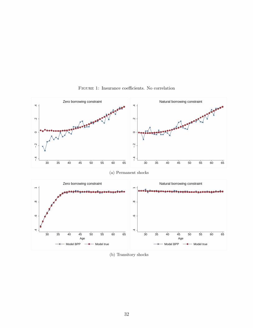
Figure 1: Insurance coefficients. No correlation
−.4
−.2
0.2
.4
30 35 40 45 50 55 60 65
Zero borrowing constraint
−.4
−.2
0.2
.4
30 35 40 45 50 55 60 65
Natural borrowing constraint
(a) Permanent shocks
.4.6
.81
30 35 40 45 50 55 60 65
Model BPP Model true
Zero borrowing constraint
Age
.4.6
.81
30 35 40 45 50 55 60 65
Model BPP Model true
Natural borrowing constraint
Age
(b) Transitory shocks
32
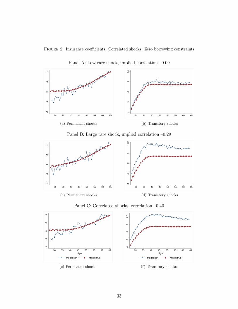
Figure 2: Insurance coefficients. Correlated shocks. Zero borrowing constraints
Panel A: Low rare shock, implied correlation –0.09
−.4
−.2
0.2
.4
30 35 40 45 50 55 60 65
(a) Permanent shocks.4
.6.8
11.
2
30 35 40 45 50 55 60 65
(b) Transitory shocks
Panel B: Large rare shock, implied correlation –0.29
−.4
−.2
0.2
.4
30 35 40 45 50 55 60 65
(c) Permanent shocks
.4.6
.81
1.2
30 35 40 45 50 55 60 65
(d) Transitory shocks
Panel C: Correlated shocks, correlation –0.40
−.4
−.2
0.2
.4
30 35 40 45 50 55 60 65
Model BPP Model true
Age
(e) Permanent shocks
.4.6
.81
1.2
30 35 40 45 50 55 60 65
Model BPP Model true
Age
(f) Transitory shocks
33
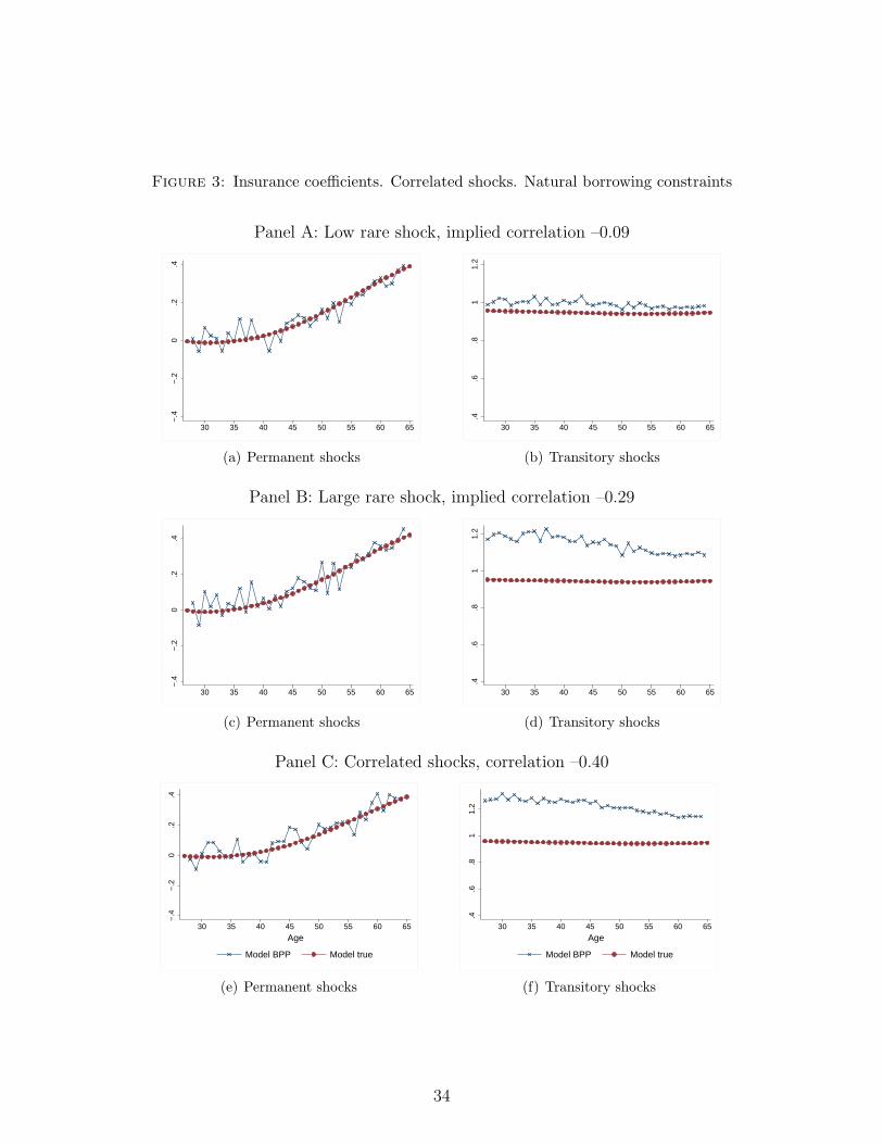
Figure 3: Insurance coefficients. Correlated shocks. Natural borrowing constraints
Panel A: Low rare shock, implied correlation –0.09
−.4
−.2
0.2
.4
30 35 40 45 50 55 60 65
(a) Permanent shocks.4
.6.8
11.
2
30 35 40 45 50 55 60 65
(b) Transitory shocks
Panel B: Large rare shock, implied correlation –0.29
−.4
−.2
0.2
.4
30 35 40 45 50 55 60 65
(c) Permanent shocks
.4.6
.81
1.2
30 35 40 45 50 55 60 65
(d) Transitory shocks
Panel C: Correlated shocks, correlation –0.40
−.4
−.2
0.2
.4
30 35 40 45 50 55 60 65
Model BPP Model true
Age
(e) Permanent shocks
.4.6
.81
1.2
30 35 40 45 50 55 60 65
Model BPP Model true
Age
(f) Transitory shocks
34
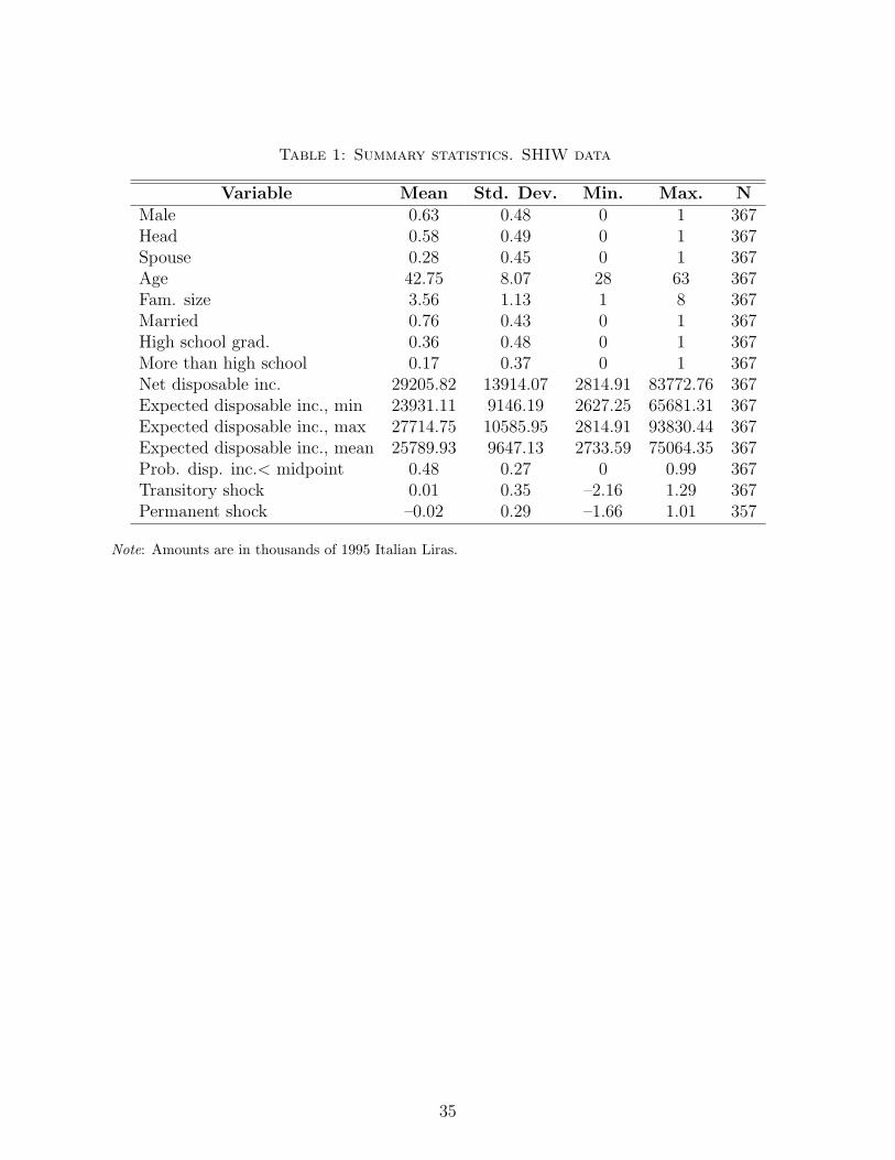
Table 1: Summary statistics. SHIW data
Variable Mean Std. Dev. Min. Max. NMale 0.63 0.48 0 1 367Head 0.58 0.49 0 1 367Spouse 0.28 0.45 0 1 367Age 42.75 8.07 28 63 367Fam. size 3.56 1.13 1 8 367Married 0.76 0.43 0 1 367High school grad. 0.36 0.48 0 1 367More than high school 0.17 0.37 0 1 367Net disposable inc. 29205.82 13914.07 2814.91 83772.76 367Expected disposable inc., min 23931.11 9146.19 2627.25 65681.31 367Expected disposable inc., max 27714.75 10585.95 2814.91 93830.44 367Expected disposable inc., mean 25789.93 9647.13 2733.59 75064.35 367Prob. disp. inc.< midpoint 0.48 0.27 0 0.99 367Transitory shock 0.01 0.35 –2.16 1.29 367Permanent shock –0.02 0.29 –1.66 1.01 357
Note: Amounts are in thousands of 1995 Italian Liras.
35
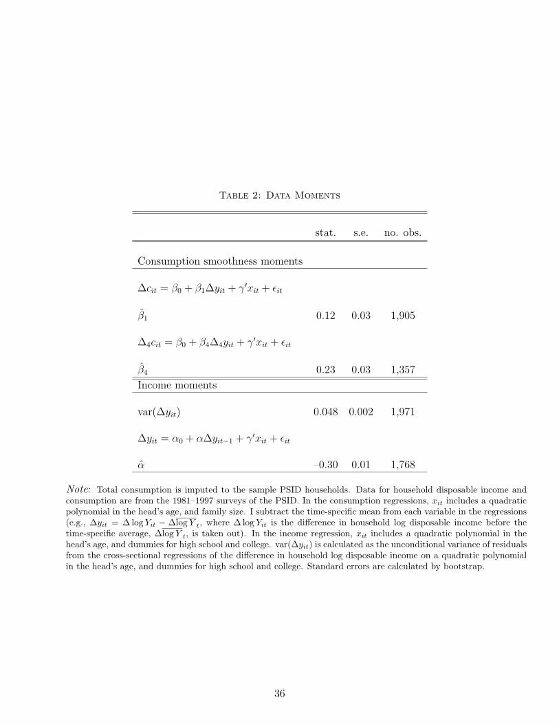
Table 2: Data Moments
stat. s.e. no. obs.
Consumption smoothness moments
∆cit = β0 + β1∆yit + γ′xit + ϵit
β1 0.12 0.03 1,905
∆4cit = β0 + β4∆4yit + γ′xit + ϵit
β4 0.23 0.03 1,357
Income moments
var(∆yit) 0.048 0.002 1,971
∆yit = α0 + α∆yit−1 + γ′xit + ϵit
α –0.30 0.01 1,768
Note: Total consumption is imputed to the sample PSID households. Data for household disposable income andconsumption are from the 1981–1997 surveys of the PSID. In the consumption regressions, xit includes a quadraticpolynomial in the head’s age, and family size. I subtract the time-specific mean from each variable in the regressions(e.g., ∆yit = ∆ log Yit − ∆log Y t, where ∆ log Yit is the difference in household log disposable income before thetime-specific average, ∆log Y t, is taken out). In the income regression, xit includes a quadratic polynomial in thehead’s age, and dummies for high school and college. var(∆yit) is calculated as the unconditional variance of residualsfrom the cross-sectional regressions of the difference in household log disposable income on a quadratic polynomialin the head’s age, and dummies for high school and college. Standard errors are calculated by bootstrap.
36
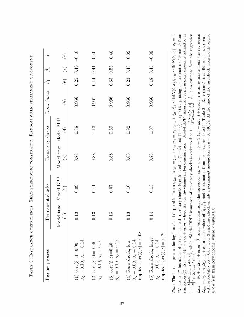
Table3:In
surancecoefficients.
Zero
borrowing
const
raint.Random
walk
permanentcomponent.
Incomeprocess
Perman
entshocks
Transitory
shocks
Disc.
factor
β1
β4
α
Model
true
Model
BPP
Model
true
Model
BPP
(1)
(2)
(3)
(4)
(5)
(6)
(7)
(8)
(1)corr(ξ,ϵ)=
0.00
0.13
0.09
0.88
0.88
0.966
0.25
0.49
–0.40
σξ=
0.10,σϵ=
0.14
(2)corr(ξ,ϵ)=
–0.40
0.13
0.11
0.88
1.13
0.967
0.14
0.41
–0.40
σξ=
0.10,σϵ=
0.16
(3)corr(ξ,ϵ)=
0.40
0.13
0.07
0.88
0.69
0.966
0.33
0.55
–0.40
σξ=
0.10,σϵ=
0.12
(4)Rareshock,low
0.13
0.10
0.88
0.92
0.966
0.23
0.48
–0.39
σξ=
0.09,σϵ=
0.14
implied
corr(ξ,ϵ)=
–0.08
(5)Rareshock,large
0.14
0.13
0.88
1.07
0.966
0.18
0.45
–0.39
σξ=
0.04,σϵ=
0.14
implied
corr(ξ,ϵ)=
–0.29
Note:Theincomeprocess
forloghou
seholddisposab
leincome,y it,isy it=pit+ϵ it,pit=ρppit−1+ξ it,ξ it∼
iidN(0,σ
2 ξ),ϵ it∼
iidN(0,σ
2 ϵ),ρp=
1.
“Model
true”
insurance
ofperman
entan
dtran
sitory
shocksis
estimated
as(1
−ϕ)an
d(1
−ψ),
respectively,
usingtheestimates
ofϕan
dψ
from
regression(2):
∆c it=ϕξ it+ψϵ it+error,where∆c itisthechan
gein
logconsumption
.“M
odel
BPP”insurance
ofperman
entshocksisestimatedas
1−
E[∆cit
∑ 1 j=
−1∆yit+
j]
E[∆yit∑ 1 j
=−
1∆yit+
j],
while“M
odel
BPP”insurance
oftran
sitory
shocksis
estimated
as1−
E[∆cit∆yit+
1]
E[∆yit∆yit+
1].β1is
anestimatefrom
theregression
∆c it=β0+β1∆y it+
error;β4is
anestimatefrom
theregression
c it−c it−
4=β0+β4(yit−y it−
4)+
error;α
isan
estimatefrom
theregression
∆y it=α0+α1∆y it−
1+
error.
Thevalues
ofβ1,β4,an
dα
estimated
from
thedataarelisted
inTab
le2.
“Rareshock”is
aniideventthatoccurs
withprobab
ilitypd=
0.05
.Low
(large)rare
shock
entailsaperman
entincomeloss
ofd=
20(40)%.Atthetimeof
therare
shock,hou
seholdsreceive
κ×d%
intran
sitory
income,
whereκequals0.5.
37
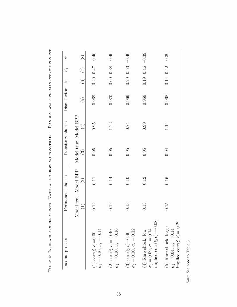
Table4:In
surancecoefficients.
Naturalborrowing
const
raint.Random
walk
permanentcomponent.
Incomeprocess
Perman
entshocks
Transitory
shocks
Disc.
factor
β1
β4
α
Model
true
Model
BPP
Model
true
Model
BPP
(1)
(2)
(3)
(4)
(5)
(6)
(7)
(8)
(1)corr(ξ,ϵ)=
0.00
0.12
0.11
0.95
0.95
0.969
0.20
0.47
–0.40
σξ=
0.10,σϵ=
0.14
(2)corr(ξ,ϵ)=
–0.40
0.12
0.14
0.95
1.22
0.970
0.09
0.38
–0.40
σξ=
0.10,σϵ=
0.16
(3)corr(ξ,ϵ)=
0.40
0.13
0.10
0.95
0.74
0.966
0.29
0.53
–0.40
σξ=
0.10,σϵ=
0.12
(4)Rareshock,low
0.13
0.12
0.95
0.99
0.969
0.19
0.46
–0.39
σξ=
0.09,σϵ=
0.14
implied
corr(ξ,ϵ)=
–0.08
(5)Rareshock,large
0.15
0.16
0.94
1.14
0.968
0.14
0.42
–0.39
σξ=
0.04,σϵ=
0.14
implied
corr(ξ,ϵ)=
–0.29
Note:See
noteto
Tab
le3.
38
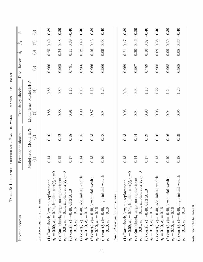
Table5:In
surancecoefficients.
Random
walk
permanentcomponent.
Incomeprocess
Perman
entshocks
Transitory
shocks
Disc.
factor
β1
β4
α
Model
true
Model
BPP
Model
true
Model
BPP
(1)
(2)
(3)
(4)
(5)
(6)
(7)
(8)
Zeroborrow
ingconstraint
(1)Rareshock,low,noreplacement
0.14
0.10
0.88
0.88
0.966
0.25
0.49
–0.39
σξ=
0.09,σϵ=
0.14,im
plied
corr(ξ,ϵ)=
0
(2)Rareshock,large,
noreplacement
0.15
0.12
0.88
0.89
0.965
0.24
0.48
–0.39
σξ=
0.04,σϵ=
0.14,im
plied
corr(ξ,ϵ)=
0
(3)corr(ξ,ϵ)=
–0.40,
CRRA
100.17
0.18
0.91
1.15
0.791
0.11
0.39
–0.40
σξ=
0.10,σϵ=
0.16
(4)corr(ξ,ϵ)=
–0.40,
addinitialwealth
0.14
0.15
0.90
1.16
0.966
0.12
0.40
–0.40
σξ=
0.10,σϵ=
0.16
(5)corr(ξ,ϵ)=
–0.40,
low
initialwealth
0.13
0.13
0.87
1.12
0.966
0.16
0.43
–0.39
σξ=
0.10,σϵ=
0.16
(6)corr(ξ,ϵ)=
–0.40,
highinitialwealth
0.16
0.18
0.94
1.20
0.966
0.09
0.38
–0.40
σξ=
0.10,σϵ=
0.16
Naturalborrow
ingconstraint
(1)Rareshock,low,noreplacement
0.13
0.13
0.95
0.94
0.969
0.21
0.47
–0.39
σξ=
0.09,σϵ=
0.14,im
plied
corr(ξ,ϵ)=
0
(2)Rareshock,large,
noreplacement
0.14
0.14
0.94
0.94
0.967
0.20
0.46
–0.39
σξ=
0.04,σϵ=
0.14,im
plied
corr(ξ,ϵ)=
0
(3)corr(ξ,ϵ)=
–0.40,
CRRA
100.17
0.19
0.93
1.18
0.789
0.10
0.37
–0.40
σξ=
0.10,σϵ=
0.16
(4)corr(ξ,ϵ)=
–0.40,
addinitialwealth
0.13
0.16
0.95
1.22
0.968
0.09
0.38
–0.40
σξ=
0.10,σϵ=
0.16
(5)corr(ξ,ϵ)=
–0.40,
low
initialwealth
0.10
0.16
0.94
1.24
0.968
0.09
0.39
–0.39
σξ=
0.10,σϵ=
0.16
(6)corr(ξ,ϵ)=
–0.40,
highinitialwealth
0.18
0.19
0.95
1.20
0.968
0.08
0.36
–0.40
σξ=
0.10,σϵ=
0.16
Note:See
noteto
Tab
le3.
39

Table6:In
surancecoefficients.
AR(1)permanentcomponent.
Incomeprocess
Persistentshocks
Transitory
shocks
Disc.
factor
β1
β4
α
Model
true
Model
BPP
Model
true
Model
BPP
(1)
(2)
(3)
(4)
(5)
(6)
(7)
(8)
Zeroborrow
ingconstraint
(1)AR(1),pers.
0.99,corr(ξ,ϵ)=
0.00
0.20
0.16
0.86
0.85
0.960
0.31
0.55
–0.35
σξ=
0.12,σϵ=
0.13
(2)AR(1),pers.
0.99,corr(ξ,ϵ)=
–0.40
0.23
0.19
0.87
1.15
0.961
0.20
0.48
–0.35
σξ=
0.12,σϵ=
0.16
(3)AR(1),pers.
0.95,corr(ξ,ϵ)=
0.00
0.32
0.31
0.83
0.62
0.944
0.60
0.66
–0.10
σξ=
0.20,σϵ=
0.06
(4)AR(1),pers.
0.95,corr(ξ,ϵ)=
–0.40
0.32
0.33
0.82
1.57
0.945
0.49
0.62
–0.10
σξ=
0.20,σϵ=
0.11
Naturalborrow
ingconstraint
(1)AR(1),pers.
0.99,corr(ξ,ϵ)=
0.00
0.20
0.18
0.92
0.91
0.963
0.27
0.53
–0.35
σξ=
0.12,σϵ=
0.13
(2)AR(1),pers.
0.99,corr(ξ,ϵ)=
–0.40
0.22
0.22
0.94
1.26
0.967
0.14
0.44
–0.35
σξ=
0.12,σϵ=
0.16
(3)AR(1),pers.
0.95,corr(ξ,ϵ)=
0.00
0.37
0.37
0.92
0.70
0.952
0.53
0.61
–0.10
σξ=
0.20,σϵ=
0.06
(4)AR(1),pers.
0.95,corr(ξ,ϵ)=
–0.40
0.41
0.41
0.93
1.71
0.957
0.40
0.55
–0.10
σξ=
0.20,σϵ=
0.11
Note:See
noteto
Tab
le3.
40
Appendix A. Data and sample selection
The Consumer Expenditure SurveyI use CEX data on total consumer expenditures and food consumption, available at the
NBER website. The data set spans the period 1980–2003. The CEX is designed by theBureau of Labor Statistics to construct the CPI at different levels of aggregation. Thesurvey publishes at most four quarters of information on individual consumption, alongwith demographic information. The NBER extracts lump quarterly records into one annualrecord.
Total consumption is defined as household total expenditures on nondurables (food athome, food at work, food away from home, clothes, personal care items, utility payments,transportation including gasoline and insurance, recreation services, gambling and charity),household supplies and equipment, rents, medical services, vehicles and auto parts, booksand publications, education, interest payments, housing property taxes, contributions toprivate pensions and self-employed retirement. The measure is defined similarly to Blundell,Pistaferri, and Preston (2008).
Households may enter the survey in the same year but in different quarters and monthsof a quarter. If household consumption record relates both to years t and t+1, I assume thatannual consumption refers to year t if that year contains at least six months of consumptionrecords, and to year t + 1 otherwise. In the CEX, the head of a household is the personwho owns or rents the unit of household residence. In the PSID, the head of a householdis male, unless he is permanently disabled (see Hill 1992). To make the definitions of headscomparable, I assume that heads are males in the CEX families with couples.
My sample selection steps are the following. First, I keep only the households that reportexpenditures in all four quarters of the year, and who are classified as full income reporters.I further keep married couples, with heads who are not self-employed, of age above 25 butbelow 71; and with family size equal or greater than 2 family members. I drop householdswhose heads attend college, part-time or full-time; or do not have education, race, age, orstate of residence records. I also drop households that report zero expenditures on food athome. I deflate food at home, food away from home, total food as well as total household ex-penditures by the Bureau of Labor Statistics (BLS) food at home, food away, total food andall items CPI with the base 100 in 1982–1984, respectively. I use non-seasonally adjusted,U.S. city average CPI indices for March of the respective year. I further drop householdswhose expenditures on food at home and away from home exceed household disposable in-come. Household disposable income is defined as the difference between household taxableincome and federal income taxes. Household taxable income, in turn, is the sum of wages andsalaries, rents, dividends and interest, business and farm income, pensions, social securitybenefits, supplemental security income, unemployment compensation, and workers’ compen-sation for all family members. To eliminate the influence of outliers, I drop observationsbelow the 1st and above the 99th percentiles of the annual total food distributions.
I utilize information on 23,133 households whose heads are of ages 26–65 to estimatethe relationship between food consumption and total consumption. The relationship is laterused for imputation of the total consumption to the sample PSID households. I use incomeinformation for households whose heads are of ages 26–70 to estimate the deterministic profile
41
of life-cycle growth in household disposable income.
The Panel Study of Income DynamicsI use PSID data from the 1981–2003 waves, the same time span during which I have
data on consumption and demographics in the CEX. To allow for a more representativesample, I drop households that are part of the Survey of Economic Opportunity (SEO)subsample. The PSID consistently collected only two items of consumption over time: foodconsumption at home and food consumption away from home (excluding food at work).Since I am interested in total household consumption and income dynamics over the lifecycle, I impute total consumption to the PSID households. Most of the studies that usefood consumption from the PSID assume that food consumption recorded in survey year treflects the typical weekly food consumption flow in year t − 1. In this paper, I adopt thesame strategy. Over the time span considered, the PSID did not collect food consumptiondata in 1988 and 1989. Correspondingly, my final sample of analysis lacks food and totalconsumption data for 1987 and 1988. Food away from home and food at home are deflatedby their respective CPIs taken from the BLS.
The sample selection details are as follows. I first make the age series consistent through-out the survey years. An individual’s age in adjacent years can be the same or differ by morethan one year since households may be interviewed in different months of a year. I take thefirst record on age when an individual appears as the head of household and impute age inother years using that record. I then drop households whose heads are younger than 26 orolder than 70, and all female-headed households. I then choose continuously married headswith the longest spell of an uninterrupted headship. I further drop households whose headshad a spell of self-employment, and keep those who never experienced significant changes infamily composition, that is those who had no changes at all or changes in members otherthan the head or wife. I drop households with inconsistent race records (e.g., householdswhose heads report being white in one survey year and black in some other year), and house-holds with heads who become permanently disabled or continue schooling after age 26. I sethead’s education to the maximum years of schooling reported by the head during sampleyears. Heads are then assigned to three educational categories: high school dropouts (withyears of schooling below 12), high school graduates (with years of schooling above 11 but lessthan 16 years), and college graduates (with years of schooling equal to or exceeding 16 years).I further drop observations with missing records on head’s or household disposable income;with zero records on head’s income when heads are of ages 26 to 65, at their pre-retirementstage of the life cycle. I also drop income outliers and single-headed households. An in-come outlier is defined as an observation on household disposable income at time t when thegrowth rate in household disposable income between periods t−1 and t is above 500 percentor below –80 percent. I then select, for each household, the longest spell of an uninterruptedheadship with all relevant information. I keep those who were born between 1912 and 1978,and whose total food expenditures do not exceed household disposable income. I also dropobservations with household food expenditures above the 99th or below the 1st percentilesof the annual food distributions. Similar to my selection rules for the CEX sample, I dropobservations with expenditures on food at home equal to zero. In the PSID, income recordedin year t refers to income earned in year t − 1. Conformably with income observations, I
42
assume that demographic information and household food expenditures recorded in year trefer to a previous year.
Before 1994, the PSID recorded annual household expenditures on food at home or awayfrom home. In 1994, the PSID started recording food at home and food away from home atdifferent frequencies—daily, weekly, biweekly, monthly, or annual frequency. For those years,I use household food records at the monthly or weekly frequency. I lose a small number ofobservations on household food expenditures reported at other frequencies. Most of them,when converted to annual amounts, were clear outliers.
The PSID estimated household federal income taxes for 1980–1991. Starting in 1992, thePSID discontinued calculation of federal income taxes. Since my data extend well beyond1992, I use the TAXSIM tool at the NBER to calculate a consistent series of householdfederal income taxes and social security withholdings. I assume that family members otherthan the head and wife are filing their tax returns separately. Household disposable incomeis then calculated as the sum of the head’s and wife’s labor income, their combined transferincome, transfer income of all other family members, taxable income of other family membersless federal income taxes and social security withholdings for the head and wife and all otherfamily members. I also add the total family social security income for 1994–2003 to themeasure of disposable income since the records on head’s and wife’s transfer income andtransfer income of other family members exclude social security income in those years.
For the households in my final sample, I use wealth information from the 1984, 1989,1994, 1999, 2001 and 2003 wealth supplements. The wealth measure utilized is the totalhousehold net worth exclusive of household business wealth.
Imputation of ConsumptionIn this appendix, I describe the procedure used to impute total consumption to the PSID
households. Absent data on total consumption in the PSID, imputation is usually donein order to exploit the panel structure of the PSID. Skinner (1987), using the 1972–1973and 1983 waves of the CEX, showed that total household consumption tightly relates toseveral consumption items, also available in the PSID (food at home and away from home,number of vehicles owned, and housing rent). Moreover, he showed that this relationship isstable over time. Blundell, Pistaferri, and Preston (2005) pioneered a structural approachto imputation—inverting the food demand equation estimated on CEX data. They relatefood consumption to nondurable expenditures, household demographics, price indices, timedummies, cohort dummies, and nondurable expenditures interacted with time dummies andthe head’s education category. I run a similar regression, and use the coefficients fromthis regression to impute total consumption to the PSID households. In the OLS setting,the estimated elasticities may be biased due to measurement error in total expenditures,and endogeneity of food and total consumption. I therefore follow Blundell, Pistaferri, andPreston (2008), and instrument log total expenditures (and its interactions with year andeducation dummies) with the head’s and wife’s education-year-cohort specific averages of loghourly wages (and their interactions with year and education dummies). The results of anIV regression of food consumption on total expenditures are presented in Table A-1. Theestimated elasticity of food consumption with respect to total expenditures is high in the1980s, and drops steadily to about 0.60 in 2002.
43
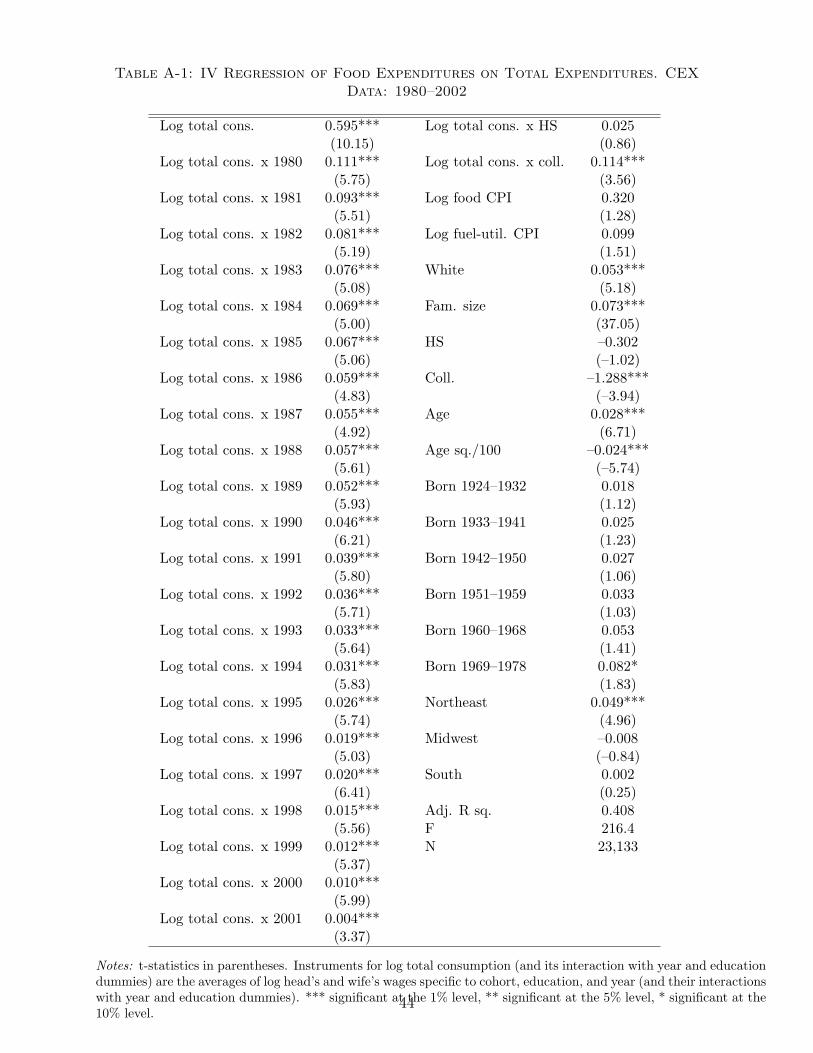
Table A-1: IV Regression of Food Expenditures on Total Expenditures. CEXData: 1980–2002
Log total cons. 0.595*** Log total cons. x HS 0.025(10.15) (0.86)
Log total cons. x 1980 0.111*** Log total cons. x coll. 0.114***(5.75) (3.56)
Log total cons. x 1981 0.093*** Log food CPI 0.320(5.51) (1.28)
Log total cons. x 1982 0.081*** Log fuel-util. CPI 0.099(5.19) (1.51)
Log total cons. x 1983 0.076*** White 0.053***(5.08) (5.18)
Log total cons. x 1984 0.069*** Fam. size 0.073***(5.00) (37.05)
Log total cons. x 1985 0.067*** HS –0.302(5.06) (–1.02)
Log total cons. x 1986 0.059*** Coll. –1.288***(4.83) (–3.94)
Log total cons. x 1987 0.055*** Age 0.028***(4.92) (6.71)
Log total cons. x 1988 0.057*** Age sq./100 –0.024***(5.61) (–5.74)
Log total cons. x 1989 0.052*** Born 1924–1932 0.018(5.93) (1.12)
Log total cons. x 1990 0.046*** Born 1933–1941 0.025(6.21) (1.23)
Log total cons. x 1991 0.039*** Born 1942–1950 0.027(5.80) (1.06)
Log total cons. x 1992 0.036*** Born 1951–1959 0.033(5.71) (1.03)
Log total cons. x 1993 0.033*** Born 1960–1968 0.053(5.64) (1.41)
Log total cons. x 1994 0.031*** Born 1969–1978 0.082*(5.83) (1.83)
Log total cons. x 1995 0.026*** Northeast 0.049***(5.74) (4.96)
Log total cons. x 1996 0.019*** Midwest –0.008(5.03) (–0.84)
Log total cons. x 1997 0.020*** South 0.002(6.41) (0.25)
Log total cons. x 1998 0.015*** Adj. R sq. 0.408(5.56) F 216.4
Log total cons. x 1999 0.012*** N 23,133(5.37)
Log total cons. x 2000 0.010***(5.99)
Log total cons. x 2001 0.004***(3.37)
Notes: t-statistics in parentheses. Instruments for log total consumption (and its interaction with year and educationdummies) are the averages of log head’s and wife’s wages specific to cohort, education, and year (and their interactionswith year and education dummies). *** significant at the 1% level, ** significant at the 5% level, * significant at the10% level.
44
Recommended