EVALUATION OF THE DESIGN LENGTH OF VERTICAL GEOTHERMAL
BOREHOLES USING ANNUAL SIMULATIONS COMBINED WITH GENOPT
Mohammadamin Ahmadfard, Michel Bernier, Michaël Kummert
Département de génie mécanique
Polytechnique Montréal [email protected], [email protected], [email protected]
ABSTRACT Software tools to determine the design length of
vertical geothermal boreholes typically use a limited set
of averaged ground thermal loads and are decoupled
from building simulations. In the present study, multi-
annual building hourly loads are used to determine the
required borehole lengths. This is accomplished within
TRNSYS using GenOpt combined with the duct
ground heat storage (DST) model for bore fields.
INTRODUCTION The determination of the required total borehole length
in a bore field is an important step in the design of
vertical ground heat exchangers (GHE) used in ground-
source heat pump (GSHP) systems. Undersized GHE may lead to system malfunction due to return fluid
temperatures that may be outside the operating limits of
the heat pumps. Oversized heat exchangers have high
installation costs that may reduce the economic
feasibility of GSHP systems.
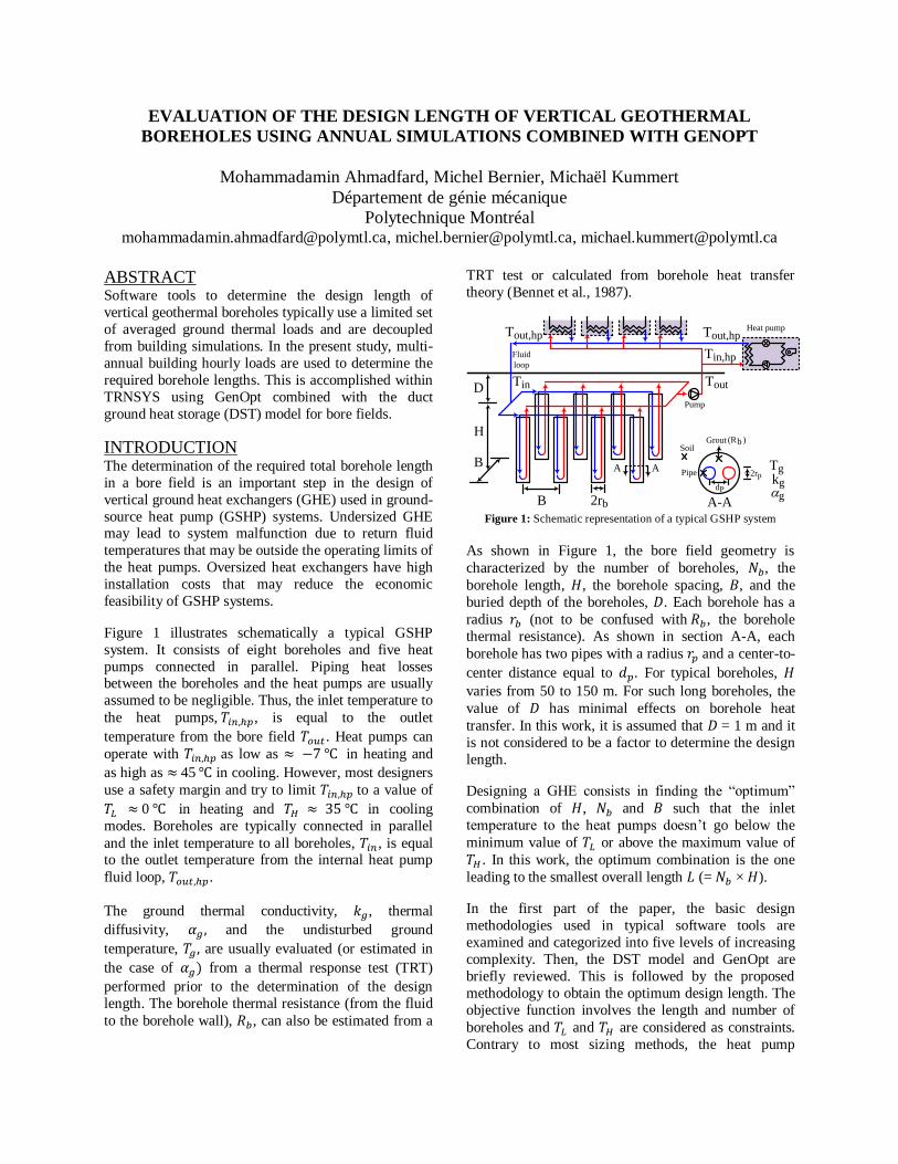
Figure 1 illustrates schematically a typical GSHP
system. It consists of eight boreholes and five heat
pumps connected in parallel. Piping heat losses between the boreholes and the heat pumps are usually
assumed to be negligible. Thus, the inlet temperature to
the heat pumps, 𝑇𝑖𝑛,ℎ𝑝, is equal to the outlet
temperature from the bore field 𝑇𝑜𝑢𝑡 . Heat pumps can
operate with 𝑇𝑖𝑛,ℎ𝑝 as low as ≈ −7 ℃ in heating and
as high as ≈ 45 ℃ in cooling. However, most designers
use a safety margin and try to limit 𝑇𝑖𝑛,ℎ𝑝 to a value of
𝑇𝐿 ≈ 0 ℃ in heating and 𝑇𝐻 ≈ 35 ℃ in cooling
modes. Boreholes are typically connected in parallel
and the inlet temperature to all boreholes, 𝑇𝑖𝑛 , is equal to the outlet temperature from the internal heat pump
fluid loop, 𝑇𝑜𝑢𝑡,ℎ𝑝.
The ground thermal conductivity, 𝑘𝑔, thermal
diffusivity, 𝛼𝑔 , and the undisturbed ground
temperature, 𝑇𝑔 , are usually evaluated (or estimated in
the case of 𝛼𝑔) from a thermal response test (TRT)
performed prior to the determination of the design
length. The borehole thermal resistance (from the fluid
to the borehole wall), 𝑅𝑏, can also be estimated from a
TRT test or calculated from borehole heat transfer
theory (Bennet et al., 1987).
Figure 1: Schematic representation of a typical GSHP system
As shown in Figure 1, the bore field geometry is
characterized by the number of boreholes, 𝑁𝑏, the
borehole length, 𝐻, the borehole spacing, 𝐵, and the
buried depth of the boreholes, 𝐷. Each borehole has a
radius 𝑟𝑏 (not to be confused with 𝑅𝑏, the borehole
thermal resistance). As shown in section A-A, each
borehole has two pipes with a radius 𝑟𝑝 and a center-to-
center distance equal to 𝑑𝑝. For typical boreholes, 𝐻
varies from 50 to 150 m. For such long boreholes, the
value of 𝐷 has minimal effects on borehole heat
transfer. In this work, it is assumed that 𝐷 = 1 m and it
is not considered to be a factor to determine the design
length.
Designing a GHE consists in finding the “optimum”
combination of 𝐻, 𝑁𝑏 and 𝐵 such that the inlet
temperature to the heat pumps doesn’t go below the
minimum value of 𝑇𝐿 or above the maximum value of
𝑇𝐻 . In this work, the optimum combination is the one
leading to the smallest overall length 𝐿 (= 𝑁𝑏 × 𝐻).
In the first part of the paper, the basic design
methodologies used in typical software tools are
examined and categorized into five levels of increasing
complexity. Then, the DST model and GenOpt are
briefly reviewed. This is followed by the proposed
methodology to obtain the optimum design length. The
objective function involves the length and number of
boreholes and 𝑇𝐿 and 𝑇𝐻 are considered as constraints.
Contrary to most sizing methods, the heat pump
H
B
DTin Tout
Tgkg
g
A A
Heat pump
A-A
Pipe
GroutSoil
Fluid
loop
Pump
Tin,hp
Tout,hp
(R )b
B
Tout,hp
2rb
2rp
dP
Coefficient of Performance (COP) is considered
variable and so the ground loads are determined
iteratively. Finally, the proposed methodology is
applied and compared to other design software tools in
three test cases.
REVIEW OF DESIGN METHODOLOGIES Spitler and Bernier (2016) categorized GHE sizing
methodologies into five levels (0 to 4) of increasing
complexity. The proposed methodology fits into the
“level 4” category. These various levels will now be
described with an emphasis on level 4.
Level 0 – Rules-of-Thumb
Rules-of-thumb relate the length of GHEs to the largest
heating or cooling loads of the building or to the
installed heat pump capacity. One popular rule-of-
thumb in North America is to determine the length
based on the simple formula: 150 feet of bore per ton of
installed capacity (13 m of bore per kW of installed capacity). In the United Kingdom, look-up tables are
used to obtain the maximum power that can be
extracted per unit length for various ground conditions
(Department of Energy and Climate Change, 2011).
For example, for 𝑘𝑔 = 2.5 W/m-K and 𝑇𝑔 = 12 °C , the
recommended maximum power extraction is 50 W/m
for 1200 hours of equivalent full load operating hours.
The main problem with rules-of-thumb is that they only
rely on peak loads and do not account for annual
ground temperature increases (decreases) caused by load thermal imbalances.
Level 1 – Two ground load pulses
In level l methods, two lengths are calculated based on
peak heating and cooling loads. Kavanaugh (1991) introduced a borehole thermal resistance in the analysis
as well as an approximate factor to account for
borehole-to-borehole thermal interference.
Furthermore, the concept of temperature limits (𝑇𝐿 and
𝑇𝐻 ) is introduced. Despite these improvements, level 1
methods suffer from the same problem as level 0
methods as they do not properly account for the effects
of ground load thermal imbalances.
Level 2 – Two set of three ground load pulses
The three pulse methodology (3 pulses in heating and 3
in cooling) is introduced by Kavanaugh (1995) along
with the concept of temporal superposition which leads
to the development of Eq.1. In order to keep the
analysis simple, the borehole thermal resistance is assumed to be negligible and so it has been eliminated
from the equation (it will be reintroduced later). In this
equation, 𝐿 is the overall borehole length (= 𝐻 × 𝑁𝐵),
𝑘 is the ground thermal conductivity, 𝑇𝑓 is the mean
fluid temperature (= [𝑇𝑖𝑛,ℎ𝑝+𝑇𝑜𝑢𝑡,ℎ𝑝]/2) and 𝑇𝑔 is the
ground temperature. The temperature penalty, 𝑇𝑝,
accounts for the borehole-to-borehole thermal
interference (Bernier et al., 2008). 𝑄1, 𝑄2, and 𝑄3 are three consecutive ground load “pulses” with time
durations 𝑡1, 𝑡2, 𝑡3. The values of 𝑡1′ , 𝑡2
′ and 𝑡3′ are
equal to 𝑡1, 𝑡1 + 𝑡2, and 𝑡1 + 𝑡2 + 𝑡3, respectively
Finally, the function ᴦ𝐺 is the thermal response of the
ground which can be evaluated using several
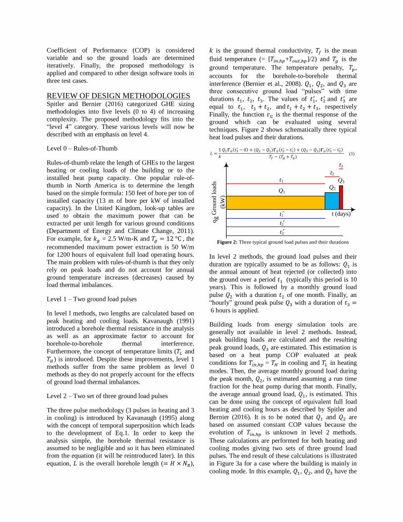
techniques. Figure 2 shows schematically three typical
heat load pulses and their durations.
𝐿 =1
𝑘
𝑄1ᴦ𝐺(𝑡3′ − 0) + (𝑄2 − 𝑄1)ᴦ𝐺(𝑡3
′ − 𝑡1′ ) + (𝑄3 − 𝑄2)ᴦ𝐺(𝑡3
′ − 𝑡2′ )
𝑇𝑓 − (𝑇𝑔 + 𝑇𝑝) (1)
Figure 2: Three typical ground load pulses and their durations
In level 2 methods, the ground load pulses and their
duration are typically assumed to be as follows: 𝑄1 is the annual amount of heat rejected (or collected) into
the ground over a period 𝑡1 (typically this period is 10
years). This is followed by a monthly ground load
pulse 𝑄2 with a duration 𝑡2 of one month. Finally, an
“hourly” ground peak pulse 𝑄3 with a duration of 𝑡3 = 6 hours is applied.
Building loads from energy simulation tools are
generally not available in level 2 methods. Instead,
peak building loads are calculated and the resulting
peak ground loads, 𝑄3 are estimated. This estimation is
based on a heat pump COP evaluated at peak
conditions for 𝑇𝑖𝑛,ℎ𝑝 = 𝑇𝐻 in cooling and 𝑇𝐿 in heating
modes. Then, the average monthly ground load during
the peak month, 𝑄2, is estimated assuming a run time
fraction for the heat pump during that month. Finally,
the average annual ground load, 𝑄1, is estimated. This
can be done using the concept of equivalent full load
heating and cooling hours as described by Spitler and
Bernier (2016). It is to be noted that 𝑄1 and 𝑄2 are
based on assumed constant COP values because the
evolution of 𝑇𝑖𝑛,ℎ𝑝 is unknown in level 2 methods.
These calculations are performed for both heating and
cooling modes giving two sets of three ground load
pulses. The end result of these calculations is illustrated
in Figure 3a for a case where the building is mainly in
cooling mode. In this example, 𝑄1, 𝑄2, and 𝑄3 have the
qg
Gro
und l
oad
s
(kW
)
t (days)
Q1Q2
Q3t1
t2
t3
t1
t2
t3
following values: 19.2, 41.9, and 139.7 kW. These
values are used in a test case to be examined shortly.
Figure 3: Typical ground loads related to level 2 sizing methods and
the variation of 𝑇𝑜𝑢𝑡 related to these loads
Eq. 1 forms the basis of the ASHRAE sizing method
(ASHRAE, 2015) where ᴦ𝐺 is based on the analytical
solution to ground heat transfer referred to as the
infinite cylindrical heat source or ICS (Bernier, 2000).
Approximate values of 𝑇𝑝 are tabulated for typical
cases in the ASHRAE handbook (ASHRAE, 2015).
Since the ICS and the tabulated values of 𝑇𝑝 are
independent of 𝐻, then 𝐿 can be determined directly
without iterations. The resulting value of 𝐿 is the length
required for the outlet temperature from the borehole,
𝑇𝑜𝑢𝑡 , to remain below 𝑇𝐻 (or above 𝑇𝐿 for a heating
case). This is illustrated in Figure 3b. This figure shows
the evolution of 𝑇𝑜𝑢𝑡 for the three ground load pulses of
Figure 3a and shows that 𝑇𝑜𝑢𝑡 reaches 𝑇𝐻 at 𝑡3′ .
If more precise values of 𝑇𝑝 are required in Eq. 1, then
the approach suggested by Bernier et al. (2008) should
be used. However, in this case 𝑇𝑝 depends on 𝐻, and
iterations are required to determine 𝐿. Typically, 3-4
iterations are necessary before convergence. This can
be done for rectangular bore fields automatically and
rapidly with the Excel spreadsheet developed by
Philippe et. al. (2010).
As suggested by Ahmadfard and Bernier (2014), the
thermal response ᴦ𝐺 in Eq. 1 can also be based on
Eskilson’s g-function (Eskilson, 1987). With this
approach the temperature penalty, 𝑇𝑝, is no longer
needed and Eq. 1 takes the following form where ᴦ𝑔 is
determined by the g-function of the bore field:
𝐿 =1
2𝜋𝑘
𝑄1ᴦ𝑔(𝑡3′ − 0) + (𝑄2 − 𝑄1)ᴦ𝑔(𝑡3
′ − 𝑡1′ ) + (𝑄3 − 𝑄2)ᴦ𝑔(𝑡3
′ − 𝑡2′ )
𝑇𝑓 − 𝑇𝑔
(2)
Since g-functions depend on 𝐻, an iterative process is
required. This process can be computationally intensive
if g-functions need to be evaluated during the process.
Pre-calculated g-functions can be used to reduce
computational time.
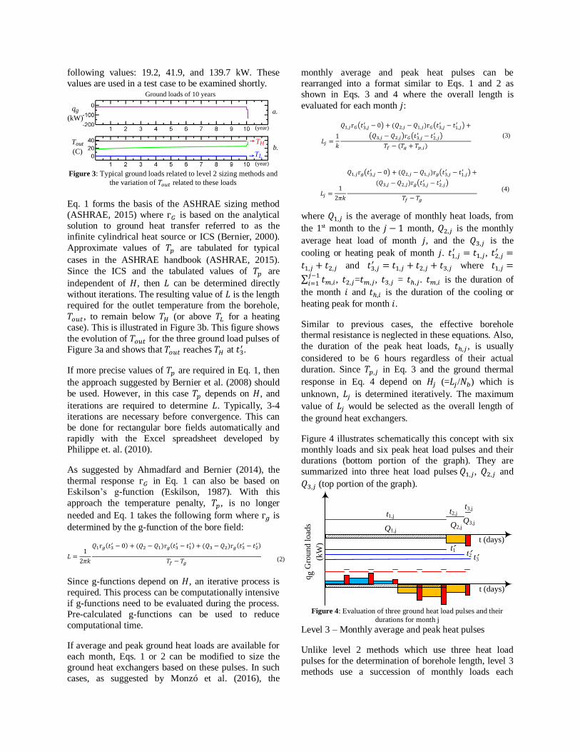
If average and peak ground heat loads are available for
each month, Eqs. 1 or 2 can be modified to size the
ground heat exchangers based on these pulses. In such
cases, as suggested by Monzó et al. (2016), the
monthly average and peak heat pulses can be
rearranged into a format similar to Eqs. 1 and 2 as
shown in Eqs. 3 and 4 where the overall length is
evaluated for each month 𝑗:
𝐿𝑗 =1
𝑘
𝑄1,𝑗ᴦ𝐺(𝑡3,𝑗′ − 0) + (𝑄2,𝑗 − 𝑄1,𝑗)ᴦ𝐺(𝑡3,𝑗
′ − 𝑡1,𝑗′ ) +
(𝑄3,𝑗 − 𝑄2,𝑗)ᴦ𝐺(𝑡3,𝑗′ − 𝑡2,𝑗
′ )
𝑇𝑓 − (𝑇𝑔 + 𝑇𝑝,𝑗)
(3)
𝐿𝑗 =1
2𝜋𝑘
𝑄1,𝑗ᴦ𝑔(𝑡3,𝑗′ − 0) + (𝑄2,𝑗 − 𝑄1,𝑗)ᴦ𝑔(𝑡3,𝑗
′ − 𝑡1,𝑗′ ) +
(𝑄3,𝑗 − 𝑄2,𝑗)ᴦ𝑔(𝑡3,𝑗′ − 𝑡2,𝑗
′ )
𝑇𝑓 − 𝑇𝑔
(4)
where 𝑄1,𝑗 is the average of monthly heat loads, from
the 1st month to the 𝑗 − 1 month, 𝑄2,𝑗 is the monthly
average heat load of month 𝑗, and the 𝑄3,𝑗 is the
cooling or heating peak of month 𝑗. 𝑡1,𝑗′ = 𝑡1,𝑗, 𝑡2,𝑗
′ =
𝑡1,𝑗 + 𝑡2,𝑗 and 𝑡3,𝑗′ = 𝑡1,𝑗 + 𝑡2,𝑗 + 𝑡3,𝑗 where 𝑡1,𝑗 =
∑ 𝑡𝑚,𝑖𝑗−1𝑖=1 , 𝑡2,𝑗=𝑡𝑚,𝑗, 𝑡3,𝑗 = 𝑡ℎ,𝑗. 𝑡𝑚,𝑖 is the duration of
the month 𝑖 and 𝑡ℎ,𝑖 is the duration of the cooling or
heating peak for month 𝑖.
Similar to previous cases, the effective borehole thermal resistance is neglected in these equations. Also,
the duration of the peak heat loads, 𝑡ℎ,𝑗 , is usually
considered to be 6 hours regardless of their actual
duration. Since 𝑇𝑝,𝑗 in Eq. 3 and the ground thermal
response in Eq. 4 depend on 𝐻𝑗 (=𝐿𝑗/𝑁𝑏) which is
unknown, 𝐿𝑗 is determined iteratively. The maximum
value of 𝐿𝑗 would be selected as the overall length of
the ground heat exchangers.
Figure 4 illustrates schematically this concept with six
monthly loads and six peak heat load pulses and their
durations (bottom portion of the graph). They are
summarized into three heat load pulses 𝑄1,𝑗, 𝑄2,𝑗 and
𝑄3,𝑗 (top portion of the graph).
Figure 4: Evaluation of three ground heat load pulses and their
durations for month j
Level 3 – Monthly average and peak heat pulses
Unlike level 2 methods which use three heat load
pulses for the determination of borehole length, level 3
methods use a succession of monthly loads each
TL
TH
Ground loads of 10 years
qg
(kW)
Tout (C)
a.
b.
(year)
(year)
qg
Gro
un
d l
oad
s
(kW
) t (days)
t1,j
t1t2 t3
t2,jt3,j
Q1,jQ2,j
Q3,j
t (days)
followed by a peak load at the end of the month. This
results in 24𝑛 terms where 𝑛 is the number of years
covered by the analysis. In level 2 methods, a fixed
value of 𝑇𝑓 is used to obtain 𝐿 directly (or with some
iterations if improved values of 𝑇𝑝 are used). However,
in level 3 methods, 𝐿 is fixed and 𝑇𝑓 is evaluated after
each of the 24𝑛 ground heat pulses.
Eqs. 5 and 6 show the governing equations for level 3
methods. In this case, 𝑇𝑓 is evaluated at the end of a 10
year analysis. Therefore, the numerator consists of a
summation of 240 terms. Eq.5 is used when the ground
thermal response is given by the ICS while Eq.6 is used
when g-functions are used.
𝑇𝑓 = (𝑇𝑔 + 𝑇𝑝) +
𝑄1ᴦ𝐺(𝑡240′ − 0) + (𝑄2 − 𝑄1)ᴦ𝐺(𝑡240
′ − 𝑡1′ ) + (𝑄3 − 𝑄2)ᴦ𝐺(𝑡240
′ − 𝑡2′ ) +
… + (𝑄239 − 𝑄238)ᴦ𝐺(𝑡240′ − 𝑡238
′ ) + (𝑄240 − 𝑄239)ᴦ𝐺(𝑡240′ − 𝑡239
′ )
𝑘𝐿
(5)
𝑇𝑓 = 𝑇𝑔 +
𝑄1ᴦ𝑔(𝑡240′ − 0) + (𝑄2 − 𝑄1)ᴦ𝑔(𝑡240
′ − 𝑡1′ ) + (𝑄3 − 𝑄2)ᴦ𝑔(𝑡240
′ − 𝑡2′ ) +
… + (𝑄239 − 𝑄238)ᴦ𝑔(𝑡240′ − 𝑡238
′ ) + (𝑄240 − 𝑄239)ᴦ𝑔(𝑡240′ − 𝑡239
′ )
2𝜋𝑘𝐿
(6)
In Eqs. 5 and 6, 𝑡𝑛′ = ∑ 𝑡𝑖
𝑛𝑖=1 and 𝑡𝑖 is the duration of
load 𝑄𝑖 .
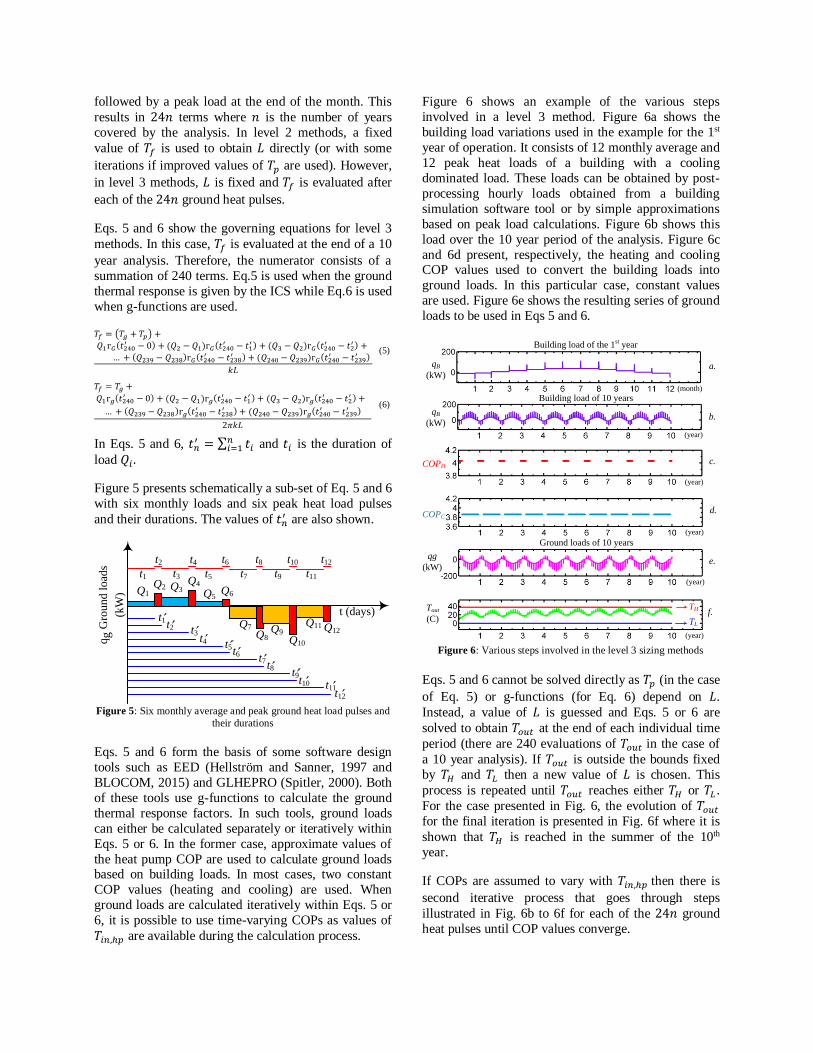
Figure 5 presents schematically a sub-set of Eq. 5 and 6
with six monthly loads and six peak heat load pulses
and their durations. The values of 𝑡𝑛′ are also shown.
Figure 5: Six monthly average and peak ground heat load pulses and
their durations
Eqs. 5 and 6 form the basis of some software design
tools such as EED (Hellström and Sanner, 1997 and
BLOCOM, 2015) and GLHEPRO (Spitler, 2000). Both
of these tools use g-functions to calculate the ground
thermal response factors. In such tools, ground loads
can either be calculated separately or iteratively within
Eqs. 5 or 6. In the former case, approximate values of
the heat pump COP are used to calculate ground loads based on building loads. In most cases, two constant
COP values (heating and cooling) are used. When
ground loads are calculated iteratively within Eqs. 5 or
6, it is possible to use time-varying COPs as values of
𝑇𝑖𝑛,ℎ𝑝 are available during the calculation process.
Figure 6 shows an example of the various steps
involved in a level 3 method. Figure 6a shows the
building load variations used in the example for the 1st
year of operation. It consists of 12 monthly average and
12 peak heat loads of a building with a cooling
dominated load. These loads can be obtained by post-
processing hourly loads obtained from a building
simulation software tool or by simple approximations
based on peak load calculations. Figure 6b shows this
load over the 10 year period of the analysis. Figure 6c
and 6d present, respectively, the heating and cooling COP values used to convert the building loads into
ground loads. In this particular case, constant values
are used. Figure 6e shows the resulting series of ground
loads to be used in Eqs 5 and 6.
Figure 6: Various steps involved in the level 3 sizing methods
Eqs. 5 and 6 cannot be solved directly as 𝑇𝑝 (in the case
of Eq. 5) or g-functions (for Eq. 6) depend on 𝐿.
Instead, a value of 𝐿 is guessed and Eqs. 5 or 6 are
solved to obtain 𝑇𝑜𝑢𝑡 at the end of each individual time
period (there are 240 evaluations of 𝑇𝑜𝑢𝑡 in the case of
a 10 year analysis). If 𝑇𝑜𝑢𝑡 is outside the bounds fixed
by 𝑇𝐻 and 𝑇𝐿 then a new value of 𝐿 is chosen. This
process is repeated until 𝑇𝑜𝑢𝑡 reaches either 𝑇𝐻 or 𝑇𝐿 .
For the case presented in Fig. 6, the evolution of 𝑇𝑜𝑢𝑡
for the final iteration is presented in Fig. 6f where it is
shown that 𝑇𝐻 is reached in the summer of the 10th
year.
If COPs are assumed to vary with 𝑇𝑖𝑛,ℎ𝑝 then there is
second iterative process that goes through steps
illustrated in Fig. 6b to 6f for each of the 24𝑛 ground
heat pulses until COP values converge.
qg
Gro
und l
oad
s
(kW
)
t (days)
Q3 Q5Q6
t1
t1t2 t3
Q1Q2
Q4
t2
t3
t4
t5
t6
t4 t5t6
Q9
Q10
Q12Q8
Q7 Q11
t7
t8
t9
t10
t11
t12
t7t8
t9t10 t11
t12
TL
TH
Building load of 10 years
qB
(kW)
Ground loads of 10 years
qg
(kW)
Tout
(C)
COPC
b.
a.
c.
d.
e.
qB
(kW)
Building load of the 1st year
(month)
(year)
(year)
(year)
(year)
COPH
f.
(year)
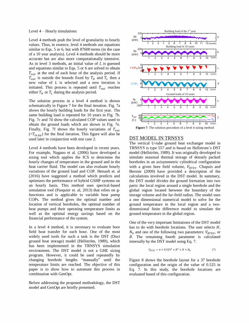
Level 4 – Hourly simulations
Level 4 methods push the level of granularity to hourly
values. Thus, in essence, level 4 methods use equations
similar to Eqs. 5 or 6, but with 87600 terms (in the case
of a 10 year analysis). Level 4 methods should be more
accurate but are also more computationally intensive.
As in level 3 methods, an initial value of 𝐿 is guessed and equations similar to Eqs. 5 or 6 are solved to obtain
𝑇𝑜𝑢𝑡 at the end of each hour of the analysis period. If
𝑇𝑜𝑢𝑡 is outside the bounds fixed by 𝑇𝐻 and 𝑇𝐿 then a
new value of 𝐿 is selected and a new iteration is
initiated. This process is repeated until 𝑇𝑜𝑢𝑡 reaches
either 𝑇𝐻 or 𝑇𝐿 during the analysis period.
The solution process in a level 4 method is shown
schematically in Figure 7 for the final iteration. Fig. 7a
shows the hourly building loads for the first year. The
same building load is repeated for 10 years in Fig. 7b.
Fig. 7c and 7d show the calculated COP values used to
obtain the ground loads which are shown in Fig. 7e.
Finally, Fig. 7f shows the hourly variations of 𝑇𝑜𝑢𝑡
(=𝑇𝑖𝑛,ℎ𝑝) for the final iteration. This figure will also be
used later in conjunction with test case 2.
Level 4 methods have been developed in recent years.
For example, Nagano et al. (2006) have developed a
sizing tool which applies the ICS to determine the hourly changes of temperature in the ground and in the
heat carrier fluid. The model can also evaluate hourly
variations of the ground load and COP. Henault et. al
(2016) have suggested a method which predicts and
optimizes the performance of hybrid GSHP systems on
an hourly basis. This method uses spectral-based
simulation tool (Pasquier et. al, 2013) that relies on g-
functions and is applicable to variable heat pump
COPs. The method gives the optimal number and
location of vertical boreholes, the optimal number of
heat pumps and their operating temperature limits as
well as the optimal energy savings based on the financial performance of the system.
In a level 4 method, it is necessary to evaluate bore
field heat transfer for each hour. One of the most
widely used tools for such a task is the DST (Duct
ground heat storage) model (Hellström, 1989), which
has been implemented in the TRNSYS simulation
environment. The DST model is not a GHE sizing program. However, it could be used repeatedly by
changing borehole lengths “manually” until the
temperature limits are reached. The objective of this
paper is to show how to automate this process in
combination with GenOpt.
Before addressing the proposed methodology, the DST
model and GenOpt are briefly presented.
Figure 7: The solution procedure of a level 4 sizing method
DST MODEL IN TRNSYS
The vertical U-tube ground heat exchanger model in
TRNSYS is type 557 and is based on Hellstrom’s DST
model (Hellström, 1989). It was originally developed to simulate seasonal thermal storage of densely packed
boreholes in an axisymmetric cylindrical configuration
with a given bore field volume, 𝑉𝐵𝑇𝐸𝑆. Chapuis and
Bernier (2009) have provided a description of the
calculations involved in the DST model. In summary,
the DST model divides the ground formation into two
parts: the local region around a single borehole and the
global region located between the boundary of the
storage volume and the far-field radius. The model uses
a one dimensional numerical model to solve for the
ground temperature in the local region and a two-dimensional finite difference model to simulate the
ground temperature in the global region.
One of the very important limitations of the DST model
has to do with borehole locations. The user selects 𝐻,
𝑁𝑏 and one of the following two parameters: 𝑉𝐵𝑇𝐸𝑆, or
𝐵. The remaining fourth parameter is calculated internally by the DST model using Eq. 7.
𝑉𝐵𝑇𝐸𝑆 = 𝜋 × 0.5252 × 𝐵2 × 𝐻 × 𝑁𝑏 (7)
Figure 8 shows the borehole layout for a 37 borehole
configuration and the origin of the value of 0.525 in
Eq. 7. In this study, the borehole locations are
evaluated based of this configuration.
TL
TH
Building load of 10 years
qB
(kW)
Ground loads of 10 years
qg
(kW)
Tout
(C)
COPC
b.
a.
c.
d.
e.
qB
(kW)
Building load of the 1st year
(month)
(year)
(year)
(year)
(year)
COPH
f.
(year)
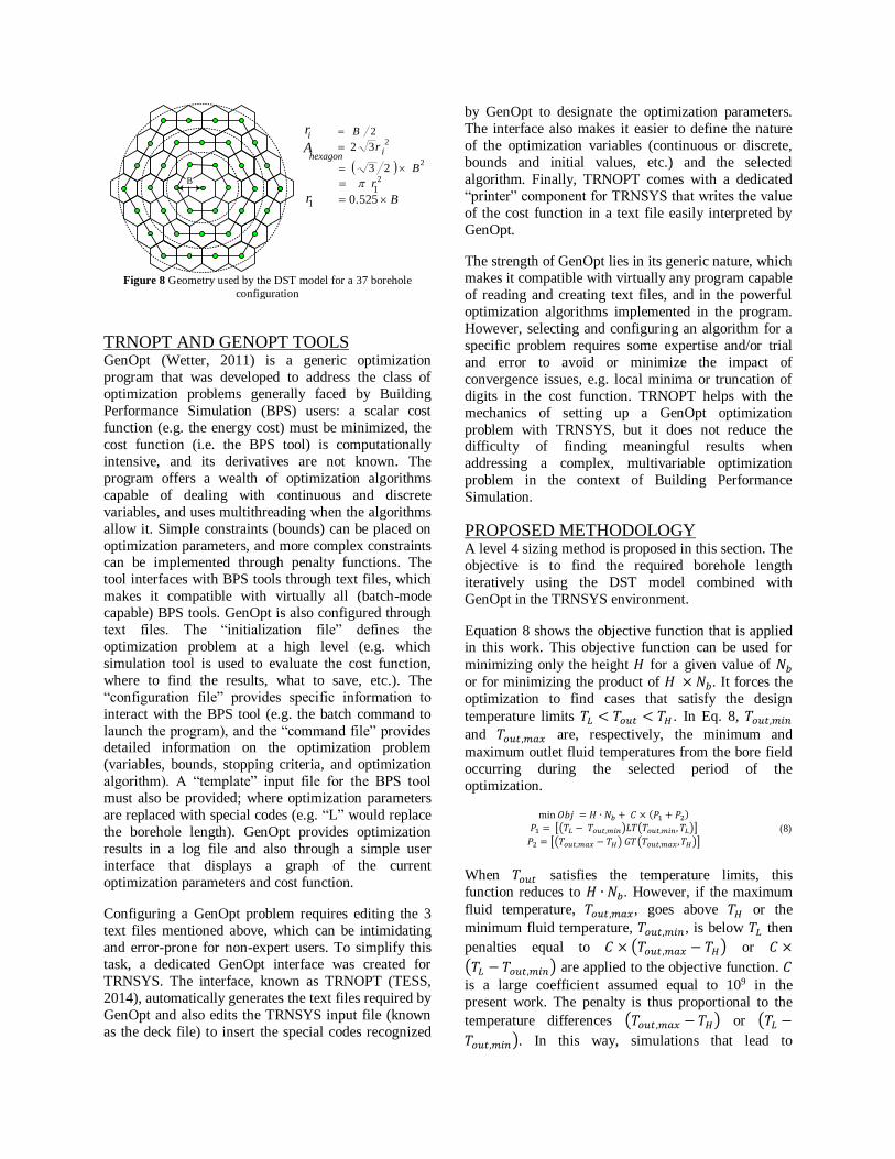
Figure 8 Geometry used by the DST model for a 37 borehole
configuration
TRNOPT AND GENOPT TOOLS
GenOpt (Wetter, 2011) is a generic optimization
program that was developed to address the class of
optimization problems generally faced by Building
Performance Simulation (BPS) users: a scalar cost
function (e.g. the energy cost) must be minimized, the
cost function (i.e. the BPS tool) is computationally
intensive, and its derivatives are not known. The
program offers a wealth of optimization algorithms
capable of dealing with continuous and discrete
variables, and uses multithreading when the algorithms
allow it. Simple constraints (bounds) can be placed on
optimization parameters, and more complex constraints can be implemented through penalty functions. The
tool interfaces with BPS tools through text files, which
makes it compatible with virtually all (batch-mode
capable) BPS tools. GenOpt is also configured through
text files. The “initialization file” defines the
optimization problem at a high level (e.g. which
simulation tool is used to evaluate the cost function,
where to find the results, what to save, etc.). The
“configuration file” provides specific information to
interact with the BPS tool (e.g. the batch command to
launch the program), and the “command file” provides detailed information on the optimization problem
(variables, bounds, stopping criteria, and optimization
algorithm). A “template” input file for the BPS tool
must also be provided; where optimization parameters
are replaced with special codes (e.g. “L” would replace
the borehole length). GenOpt provides optimization
results in a log file and also through a simple user
interface that displays a graph of the current
optimization parameters and cost function.
Configuring a GenOpt problem requires editing the 3
text files mentioned above, which can be intimidating
and error-prone for non-expert users. To simplify this
task, a dedicated GenOpt interface was created for
TRNSYS. The interface, known as TRNOPT (TESS,
2014), automatically generates the text files required by
GenOpt and also edits the TRNSYS input file (known
as the deck file) to insert the special codes recognized
by GenOpt to designate the optimization parameters.
The interface also makes it easier to define the nature
of the optimization variables (continuous or discrete,
bounds and initial values, etc.) and the selected
algorithm. Finally, TRNOPT comes with a dedicated
“printer” component for TRNSYS that writes the value
of the cost function in a text file easily interpreted by
GenOpt.
The strength of GenOpt lies in its generic nature, which
makes it compatible with virtually any program capable
of reading and creating text files, and in the powerful
optimization algorithms implemented in the program.
However, selecting and configuring an algorithm for a
specific problem requires some expertise and/or trial
and error to avoid or minimize the impact of
convergence issues, e.g. local minima or truncation of
digits in the cost function. TRNOPT helps with the
mechanics of setting up a GenOpt optimization
problem with TRNSYS, but it does not reduce the difficulty of finding meaningful results when
addressing a complex, multivariable optimization
problem in the context of Building Performance
Simulation.
PROPOSED METHODOLOGY A level 4 sizing method is proposed in this section. The
objective is to find the required borehole length
iteratively using the DST model combined with
GenOpt in the TRNSYS environment.
Equation 8 shows the objective function that is applied in this work. This objective function can be used for
minimizing only the height 𝐻 for a given value of 𝑁𝑏
or for minimizing the product of 𝐻 × 𝑁𝑏. It forces the
optimization to find cases that satisfy the design
temperature limits 𝑇𝐿 < 𝑇𝑜𝑢𝑡 < 𝑇𝐻 . In Eq. 8, 𝑇𝑜𝑢𝑡,𝑚𝑖𝑛
and 𝑇𝑜𝑢𝑡,𝑚𝑎𝑥 are, respectively, the minimum and
maximum outlet fluid temperatures from the bore field
occurring during the selected period of the
optimization.
min 𝑂𝑏𝑗 = 𝐻 ∙ 𝑁𝑏 + 𝐶 × (𝑃1 + 𝑃2)
𝑃1 = [(𝑇𝐿 − 𝑇𝑜𝑢𝑡,𝑚𝑖𝑛)𝐿𝑇(𝑇𝑜𝑢𝑡,𝑚𝑖𝑛, 𝑇𝐿)]
𝑃2 = [(𝑇𝑜𝑢𝑡,𝑚𝑎𝑥 − 𝑇𝐻) 𝐺𝑇(𝑇𝑜𝑢𝑡,𝑚𝑎𝑥, 𝑇𝐻)]
(8)
When 𝑇𝑜𝑢𝑡 satisfies the temperature limits, this
function reduces to 𝐻 ∙ 𝑁𝑏. However, if the maximum
fluid temperature, 𝑇𝑜𝑢𝑡,𝑚𝑎𝑥, goes above 𝑇𝐻 or the
minimum fluid temperature, 𝑇𝑜𝑢𝑡,𝑚𝑖𝑛 , is below 𝑇𝐿 then
penalties equal to 𝐶 × (𝑇𝑜𝑢𝑡,𝑚𝑎𝑥 − 𝑇𝐻) or 𝐶 ×
(𝑇𝐿 − 𝑇𝑜𝑢𝑡,𝑚𝑖𝑛) are applied to the objective function. 𝐶
is a large coefficient assumed equal to 109 in the
present work. The penalty is thus proportional to the
temperature differences (𝑇𝑜𝑢𝑡,𝑚𝑎𝑥 − 𝑇𝐻) or (𝑇𝐿 −
𝑇𝑜𝑢𝑡,𝑚𝑖𝑛). In this way, simulations that lead to
r32
2B
B. 5250
r
B 23B
r
1
12
i2
i
hexagonA
r
2
𝑇𝑜𝑢𝑡,𝑚𝑎𝑥 ≫ 𝑇𝐻 (or 𝑇𝑜𝑢𝑡,𝑚𝑖𝑛 ≪ 𝑇𝐿 ) will be heavily
penalized.
In Eq. 8, the expressions 𝐿𝑇(𝑇𝑜𝑢𝑡,𝑚𝑖𝑛 , 𝑇𝐿) and
𝐺𝑇(𝑇𝑜𝑢𝑡,𝑚𝑎𝑥 , 𝑇𝐻) are “lower than” and “upper than”
functions and are equal to 1 respectively
when 𝑇𝑜𝑢𝑡,𝑚𝑖𝑛 < 𝑇𝐿 and 𝑇𝑜𝑢𝑡,𝑚𝑎𝑥 > 𝑇𝐻 . For other
values these functions are zero. It should be noted that
only one of these two conditions may occur as the
system can be either be sized in heating or cooling.
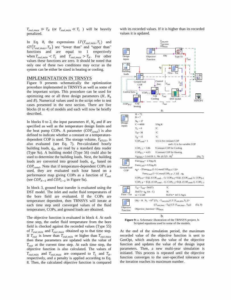
IMPLEMENTATION IN TRNSYS Figure 9 presents schematically the optimization
procedure implemented in TRNSYS as well as some of
the important scripts. This procedure can be used for
optimizing one or all three design parameters (𝐻, 𝑁𝑏
and 𝐵). Numerical values used in the script refer to test
cases presented in the next section. There are five
blocks (0 to 4) of models and each will now be briefly
described.
In blocks 0 to 2, the input parameters 𝐻, 𝑁𝑏 and 𝐵 are
specified as well as the temperature design limits and
the heat pump COPs. A parameter (𝐶𝑂𝑃𝑐𝑜𝑛𝑑) is also
defined to indicate whether a constant or a temperature-
dependent COP is used. The storage volume, 𝑉𝐵𝑇𝐸𝑆, is
also evaluated (see Eq. 7). Pre-calculated hourly
building loads, 𝑞𝑏, are read by a standard data reader
(Type 9a). A building model (Type 56) could also be
used to determine the building loads. Next, the building
loads are converted into ground loads, 𝑞𝑔, based on
𝐶𝑂𝑃𝑐𝑜𝑛𝑑 . Note that if temperature-dependent COPs are
used, they are evaluated each hour based on a
performance map giving COPs as a function of 𝑇𝑜𝑢𝑡
(see 𝐶𝑂𝑃𝐻−2 and 𝐶𝑂𝑃𝐶−2 in Figure 9a).
In block 3, ground heat transfer is evaluated using the
DST model. The inlet and outlet fluid temperatures of
the bore field are evaluated. If the COPs are
temperature dependent, then TRNSYS will iterate at
each time step until converged values of the fluid
temperature, COPs, and ground loads are obtained.
The objective function is evaluated in block 4. At each
time step, the outlet fluid temperature from the bore
field is checked against the recorded values (Type 55)
of 𝑇𝑜𝑢𝑡,𝑚𝑖𝑛 and 𝑇𝑜𝑢𝑡,𝑚𝑎𝑥 obtained up to that time step.
If 𝑇𝑜𝑢𝑡 is lower than 𝑇𝑜𝑢𝑡,𝑚𝑖𝑛 or higher than 𝑇𝑜𝑢𝑡,𝑚𝑎𝑥
then these parameters are updated with the value of
𝑇𝑜𝑢𝑡 at the current time step. At each time step, the
objective function is also calculated. The values of
𝑇𝑜𝑢𝑡,𝑚𝑖𝑛 and 𝑇𝑜𝑢𝑡,𝑚𝑎𝑥 are compared to 𝑇𝐿 and 𝑇𝐻 ,
respectively, and a penalty is applied according to Eq.
8. Then, the calculated objective function is compared
with its recorded values. If it is higher than its recorded
values it is updated.
a.
b.
Figure 9: a. Schematic illustration of the TRNSYS project, b. Scripted equations used in some of the models.
At the end of the simulation period, the maximum
recorded value of the objective function is sent to
GenOpt, which analyzes the value of the objective
function and updates the value of the design input
parameters. Then, a new multi-year simulation is
initiated. This process is repeated until the objective
function converges to the user-specified tolerance or
the iteration reaches its maximum number.
Objmax
Tout,minTout,max
DST model
Obj
1
Design
inputs
Building
loads
Objective
Function
Type 55
TRNOPT
Cop
heating
Cop
Cooling
Ground load
COP
Flow - Tin
Plotter
2
2
2
3
3
440
5
Tout
Tout
Tout
qg
Tout
Tinm
COPH-2
COPC-2Control func.
Control
func.
Design
inputs
0H = 72
B = 7
Nb = 37
C = 4000 !J/kg.K
TL = 0 !C
TH= 38 !C
Tg = 15 !C
COPcond = 1 !(1) is for constant COP
and (-1) is for variable COP
COPC-1 = 3.86 !Constant COP for Cooling
COPH-1 = 4.03 !Constant COP for Heating
VBTES = 3.14159. L. Nb. (0.525 . B)2 (Eq. 7)
FuncHeat= LT(qb,0)
FuncCool = GT(qb,0)
qg= - [FuncHeat (1-1/( max(COPH-F,1 )))+
FuncCool (1+1/( max(COPC-F ,1 )))] . qb
COPH-F= EQL (COPcond , -1). COPH-2+EQL (COPcond,1). COPH-1
COPC-F = EQL (COPcond , -1). COPC-2+EQL (COPcond,1). COPC-1
Ground load
COP
2
Tin= Tout - Del(T) !C
Del(T)= qg /(m . C) !K
m = 5.549 !0.074 * 147.5 !kg/sFlow - Tin
3
Obj = H . Nb +109 [(TL - Tout,min) LT (Tout,min,TL)]+
[(Tout,max - TH) GT (Tout,max , TH)] (Eq. 8)
Objective_function= ObjmaxObjective
Function
4
APPLICATIONS Three sizing test cases are considered in this section to
show the applicability of the proposed method and to
compare results with other sizing methods. The
reported calculation times are for a computer equipped
with an Intel core i7 processor (2.80 GHz) and 4 GB of RAM.
Test case #1
The first test case is somewhat academic as it involves
a perfectly balanced ground load. This case involves
the optimization (i.e. minimization) of 𝐻 for a 37
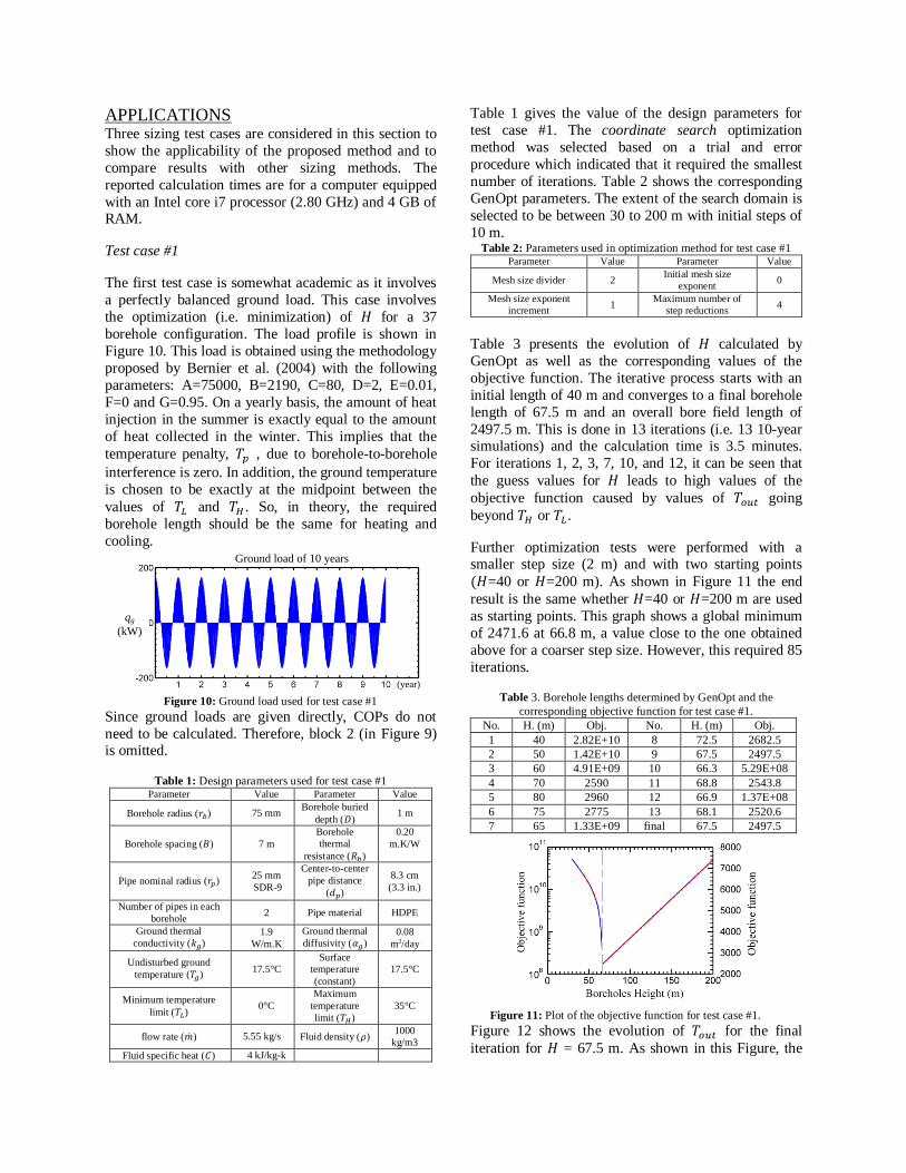
borehole configuration. The load profile is shown in
Figure 10. This load is obtained using the methodology
proposed by Bernier et al. (2004) with the following
parameters: A=75000, B=2190, C=80, D=2, E=0.01,
F=0 and G=0.95. On a yearly basis, the amount of heat
injection in the summer is exactly equal to the amount
of heat collected in the winter. This implies that the
temperature penalty, 𝑇𝑝 , due to borehole-to-borehole
interference is zero. In addition, the ground temperature
is chosen to be exactly at the midpoint between the
values of 𝑇𝐿 and 𝑇𝐻 . So, in theory, the required
borehole length should be the same for heating and
cooling.
Figure 10: Ground load used for test case #1
Since ground loads are given directly, COPs do not
need to be calculated. Therefore, block 2 (in Figure 9) is omitted.
Table 1: Design parameters used for test case #1 Parameter Value Parameter Value
Borehole radius (𝑟𝑏) 75 mm Borehole buried
depth (𝐷) 1 m
Borehole spacing (𝐵) 7 m
Borehole
thermal
resistance (𝑅𝑏)
0.20
m.K/W
Pipe nominal radius (𝑟𝑝) 25 mm
SDR-9
Center-to-center
pipe distance
(𝑑𝑝)
8.3 cm
(3.3 in.)
Number of pipes in each
borehole 2 Pipe material HDPE
Ground thermal
conductivity (𝑘𝑔) 1.9
W/m.K
Ground thermal
diffusivity (𝛼𝑔) 0.08
m2/day
Undisturbed ground
temperature (𝑇𝑔) 17.5°C
Surface
temperature
(constant)
17.5°C
Minimum temperature
limit (𝑇𝐿) 0°C
Maximum
temperature
limit (𝑇𝐻)
35°C
flow rate (�̇�) 5.55 kg/s Fluid density (𝜌) 1000
kg/m3
Fluid specific heat (𝐶) 4 kJ/kg-k
Table 1 gives the value of the design parameters for
test case #1. The coordinate search optimization
method was selected based on a trial and error
procedure which indicated that it required the smallest
number of iterations. Table 2 shows the corresponding
GenOpt parameters. The extent of the search domain is
selected to be between 30 to 200 m with initial steps of
10 m. Table 2: Parameters used in optimization method for test case #1
Parameter Value Parameter Value
Mesh size divider 2 Initial mesh size
exponent 0
Mesh size exponent
increment 1
Maximum number of
step reductions 4
Table 3 presents the evolution of 𝐻 calculated by
GenOpt as well as the corresponding values of the
objective function. The iterative process starts with an
initial length of 40 m and converges to a final borehole
length of 67.5 m and an overall bore field length of
2497.5 m. This is done in 13 iterations (i.e. 13 10-year simulations) and the calculation time is 3.5 minutes.
For iterations 1, 2, 3, 7, 10, and 12, it can be seen that
the guess values for 𝐻 leads to high values of the
objective function caused by values of 𝑇𝑜𝑢𝑡 going
beyond 𝑇𝐻 or 𝑇𝐿.
Further optimization tests were performed with a smaller step size (2 m) and with two starting points
(𝐻=40 or 𝐻=200 m). As shown in Figure 11 the end
result is the same whether 𝐻=40 or 𝐻=200 m are used
as starting points. This graph shows a global minimum
of 2471.6 at 66.8 m, a value close to the one obtained
above for a coarser step size. However, this required 85
iterations.
Table 3. Borehole lengths determined by GenOpt and the
corresponding objective function for test case #1.
No. H. (m) Obj. No. H. (m) Obj.
1 40 2.82E+10 8 72.5 2682.5
2 50 1.42E+10 9 67.5 2497.5
3 60 4.91E+09 10 66.3 5.29E+08
4 70 2590 11 68.8 2543.8
5 80 2960 12 66.9 1.37E+08
6 75 2775 13 68.1 2520.6
7 65 1.33E+09 final 67.5 2497.5
Figure 11: Plot of the objective function for test case #1.
Figure 12 shows the evolution of 𝑇𝑜𝑢𝑡 for the final
iteration for 𝐻 = 67.5 m. As shown in this Figure, the
Ground load of 10 years
qg
(kW)b.
a.qg
(kW)
Ground load of the 1st year
(month)
(year)
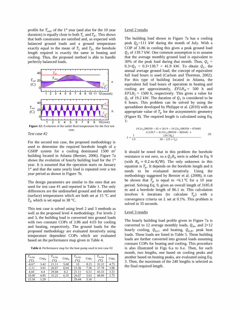
profile for 𝑇𝑜𝑢𝑡 of the 1st year (and also for the 10 year
duration) is equally close to both 𝑇𝐿 and 𝑇𝐻 . This shows
that both constraints are satisfied and, as expected with
balanced ground loads and a ground temperature
exactly equal to the mean of 𝑇𝐿 and 𝑇𝐻 , the borehole
length required is exactly the same in heating and
cooling. Thus, the proposed method is able to handle
perfectly balanced loads.
Figure 12: Evolution of the outlet fluid temperature for the first test
case. Test case #2
For the second test case, the proposed methodology is
used to determine the required borehole length of a
GSHP system for a cooling dominated 1500 m2
building located in Atlanta (Bernier, 2006). Figure 7a
shows the evolution of hourly building load for the 1st
year. It is assumed that the operation starts on January
1st and that the same yearly load is repeated over a ten
year period as shown in Figure 7b.
The design parameters are similar to the ones that are
used for test case #1 and reported in Table 1. The only
differences are the undisturbed ground and the ambient
(surface) temperatures which are both set at 15 °C and
𝑇𝐻 which is set equal to 38 °C.
This test case is solved using level 2 and 3 methods as well as the proposed level 4 methodology. For levels 2
and 3, the building load is converted into ground loads
with two constant COPs of 3.86 and 4.03 for cooling
and heating, respectively. The ground loads for the
proposed methodology are evaluated iteratively using
temperature dependent COPs which are evaluated
based on the performance map given in Table 4.
Table 4. Performance map for the heat pump used in test case #2
𝑇𝑖𝑛,ℎ𝑝
(℃) 𝐶𝑜𝑝𝐻
𝑇𝑖𝑛,ℎ𝑝
(℃) 𝐶𝑜𝑝𝐻
𝑇𝑖𝑛,ℎ𝑝
(℃) 𝐶𝑜𝑝𝐶
𝑇𝑖𝑛,ℎ𝑝
(℃) 𝐶𝑜𝑝𝐶
-6.67 3.42 21.11 5.68 10 8.15 32.22 4.75
-1.11 3.91 26.67 6.04 15.56 7.36 37.78 3.96
4.44 4.4 29.44 6.2 21.11 6.51 43.33 3.31
10.00 4.85 32.22 6.35 26.67 5.63 48.89 2.75
15.56 5.29 29.44 5.16
Level 2 results
The building load shown in Figure 7a has a cooling
peak 𝑄𝑝=111 kW during the month of July. With a
COP of 3.86 in cooling this gives a peak ground load
𝑄3 of 139.7 kW. One common assumption is to assume
that the average monthly ground load is equivalent to
30% of the peak load during that month. Thus, 𝑄2 =
0.3×𝑄3 = 0.3×139.7 = 41.9 kW. To obtain 𝑄1, the
annual average ground load, the concept of equivalent
full load hours is used (Carlson and Thornton, 2002).
For this type of building located in Atlanta, the
equivalent full load hours of operation in heating and
cooling are approximately, 𝐸𝐹𝐿𝐻𝐻 = 500 h and
𝐸𝐹𝐿𝐻𝐶 = 1500 h, respectively. This gives a value for
𝑄1 of 19.2 kW. The duration of 𝑄3 is considered to be
6 hours. This problem can be solved by using the
spreadsheet developed by Philippe et al. (2010) with an
appropriate value of 𝑇𝑝 for the axisymmetric geometry
(Figure 8). The required length is calculated using Eq. 1:
𝐿 =1
1.9
19.2ᴦ𝐺(88350 − 0) + (41.9 − 19.2)ᴦ𝐺(88350 − 87600)
+(139.7 − 41.9)ᴦ𝐺(88350 − 88344) +139.7𝑅𝑏)
38 − (15 + 𝑇𝑝)
(9)
It should be noted that in this problem the borehole
resistance is not zero, so a 𝑄3𝑅𝑏 term is added in Eq. 9
(with 𝑅𝑏 = 0.2 m-K/W). The only unknown in this
equation is 𝑇𝑝. It depends on the borehole length and it
needs to be evaluated iteratively. Using the
methodology suggested by Bernier et al. (2008), it can
be shown that 𝑇𝑝 is equal to +6.1 ℃ for a 10 year
period. Solving Eq. 9, gives an overall length of 3185.8
m and a borehole length of 86.1 m. This calculation
involves 6 iterations (to calculate 𝑇𝑝) with a
convergence criteria on L set at 0.1%. This problem is
solved in 35 seconds.
Level 3 results
The hourly building load profile given in Figure 7a is
converted to 12 average monthly loads, 𝑄𝑚, and 2×12
hourly cooling, 𝑄ℎ,𝐶, and heating, 𝑄ℎ,𝐻, peak heat
loads. These loads are listed in Table 5. These building
loads are further converted into ground loads assuming
constant COPs for heating and cooling. This procedure
is also illustrated in Figs 6.a to 6.e. Then, for each
month, two lengths, one based on cooling peaks and
another based on heating peaks, are evaluated using Eq. 3. Then, the maximum of the 240 lengths is selected as
the final required length.
TL
TH
Tout
(C)
(year)
Tmax
Tmin
(month)
Tout
(C)
TL
Tmin
TH Tmax
a.
b.
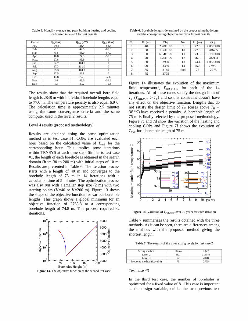
Table 5. Monthly average and peak building heating and cooling
loads used in level 3 for test case #2
Period Qm (kW) Qh,C (kW) Qh,H (kW)
Jan. -10.6 28.4 -86.4
Feb. -5.0 42.5 -80.8
Mar. 6.4 66.0 -57.9
Apr. 16.8 74.3 -50.3
May. 27.8 95.9 0
Jun. 34.7 104.0 0
Jul. 37.3 111.0 0
Aug. 35.3 104.7 0
Sep. 27.5 88.8 0
Oct. 14.8 77.3 -7.6
Nov. 2.4 42.0 -56.3
Dec. -7.8 27.2 -12.4
The results show that the required overall bore field
length is 2848 m with individual borehole lengths equal
to 77.0 m. The temperature penalty is also equal 6.9℃.
The calculation time is approximately 2.5 minutes using the same convergence criteria and the same
computer used in the level 2 results.
Level 4 results (proposed methodology)
Results are obtained using the same optimization method as in test case #1. COPs are evaluated each
hour based on the calculated value of 𝑇𝑜𝑢𝑡 for the
corresponding hour. This implies some iterations
within TRNSYS at each time step. Similar to test case
#1, the length of each borehole is obtained in the search
domain (from 30 to 200 m) with initial steps of 10 m.
Results are presented in Table 6. The iteration process
starts with a length of 40 m and converges to the
borehole length of 75 m in 14 iterations with a
calculation time of 5 minutes. The optimization process was also run with a smaller step size (2 m) with two
starting points (𝐻=40 or 𝐻=200 m). Figure 13 shows
the shape of the objective function for various borehole
lengths. This graph shows a global minimum for an
objective function of 2765.8 at a corresponding
borehole length of 74.8 m. This process required 82
iterations.
Figure 13. The objective function of the second test case.
Table 6. Borehole lengths determined by the proposed methodology
and the corresponding objective function for test case #2.
No. H. (m) Obj. No. H. (m) Obj.
1 40 2.28E+10 9 72.5 7.89E+08
2 50 1.36E+10 10 77.5 2867.5
3 60 6.64E+09 11 73.8 3.19E+08
4 70 1.76E+09 12 76.3 2821.3
5 80 2960 13 74.4 1.05E+08
6 90 3330 14 75.6 2798.1
7 85 3145 final 75 2775
8 75 2775
Figure 14 illustrates the evolution of the maximum
fluid temperature, 𝑇𝑜𝑢𝑡,𝑚𝑎𝑥, for each of the 14
iterations. All of these cases satisfy the design limit of
𝑇𝐿 (𝑇𝑜𝑢𝑡,𝑚𝑖𝑛 > 𝑇𝐿) and so this constraint doesn’t have
any effect on the objective function. Lengths that do
not satisfy the design limit of 𝑇𝐻 (cases above 𝑇𝐻 =38 °𝐶) have received a penalty. A borehole length of
75 m is finally selected by the proposed methodology.
Figure 7c and 7d show the variation of the heating and
cooling COPs and Figure 7f shows the evolution of
𝑇𝑜𝑢𝑡 for a borehole length of 75 m.
Figure 14. Variation of 𝑇𝑜𝑢𝑡,𝑚𝑎𝑥 over 10 years for each iteration
Table 7 summarizes the results obtained with the three
methods. As it can be seen, there are differences among
the methods with the proposed method giving the
shortest length.
Table 7: The results of the three sizing levels for test case 2
Sizing method H (m) L (m)
Level 2 86.1 3185.8
Level 3 77 2848
Proposed method (Level 4) 75 2775
Test case #3
In the third test case, the number of boreholes is
optimized for a fixed value of 𝐻. This case is important
as the design variable, unlike the two previous test
Boreholes Height (m)
Obje
ctiv
e fu
nct
ion
Obje
ctiv
e fu
nct
ion
40
50
60
80
90
85
8077.5
70
72.5
75.675
73.8
TL
TH
TH
TH
(year)
Max
imu
m o
utl
et f
luid
tem
per
atu
re C
74.4
76.3
cases, is a discrete variable and therefore the
coordinate search optimization method cannot be used.
For this case, the same design parameters as for the
other two cases are used. The borehole length is
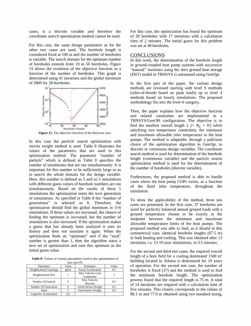
considered fixed at 100 m and the number of boreholes
is variable. The search domain for the optimum number
of boreholes extends from 10 to 50 boreholes. Figure 15 shows the evolution of the objective function as a
function of the number of boreholes. This graph is
determined using 41 iterations and the global minimum
of 2800 for 28 boreholes.
Figure 15. The objective function of the third test case.
In this case the particle swarm optimization with
inertia weight method is used. Table 8 illustrates the values of the parameters that are used in this
optimization method. The parameter “number of
particle” which is defined in Table 8 specifies the
number of simulations that are run simultaneously. It is
important for this number to be sufficiently large so as
to search the whole domain for the design variable.
Here, this number is defined as 5 and so 5 simulations
with different guess values of borehole numbers are run
simultaneously. Based on the results of these 5
simulations the optimization starts the next generation
of simulations. As specified in Table 8 the “number of generations” is selected as 6. Therefore, the
optimization should find the global minimum in 5×6
simulations. If these values are increased, the chance of
finding the optimum is increased, but the number of
simulations is also increased. If the optimization makes
a guess that has already been analyzed it uses its
history and does not simulate it again. When the
optimization finds an “optimum” and if the “seed”
number is greater than 1, then the algorithm starts a
new set of optimization and uses this optimum as the
initial guess value.
Table 8: Values of various parameters used in the optimization of
test case #3 Parameter Value Parameter Value
Neighborhood Topology gbest Social Acceleration 0.5
Neighborhood Size 1 Max Velocity Gain
Continuous 2
Number Of Particle 5 Max Velocity
Discrete 0.5
Number Of Generation 6 Initial Inertia Weight 0.5
Seed 1 Final Inertia Weight 0.5
Cognitive Acceleration 0.5
For this case, the optimization has found the optimum
of 28 boreholes with 17 iterations with a calculation
time of 2 minutes. The initial guess for this problem
was set at 40 boreholes.
CONCLUSIONS In this work, the determination of the borehole length
in ground-coupled heat pump systems with successive
“manual” iterations using the duct ground heat storage
(DST) model in TRNSYS is automated using GenOpt.
In the first part of the paper, the various design methods are reviewed starting with level 0 methods
(rules-of-thumb based on peak loads) up to level 4
methods based on hourly simulations. The proposed
methodology fits into the level 4 category.
Then, the paper explains how the objective function
and related constraints are implemented in a
TRNSYS/GenOPt configuration. The objective is to
find the smallest overall length 𝐿 (= 𝑁𝑏 × 𝐻) while satisfying two temperature constraints, the minimum
and maximum allowable inlet temperature to the heat
pumps. The method is adaptable, through a judicious
choice of the optimization algorithm in GenOpt, to
discrete or continuous design variables. The coordinate
search method is used for determination of the borehole
length (continuous variable) and the particle swarm
optimization method is used for the determination of
the number of boreholes (discrete variable).
Furthermore, the proposed method is able to handle
cases where the heat pump COPs varies, as a function
of the fluid inlet temperature, throughout the
simulation.
To show the applicability of the method, three test cases are presented. In the first case, 37 boreholes are
sized for perfectly balanced annual ground loads with a
ground temperature chosen to be exactly at the
midpoint between the minimum and maximum
allowable temperature limits of the heat pumps. The
proposed method was able to find, as it should in this
symmetrical case, identical borehole lengths (67.5 m)
in both heating and cooling. This was obtained after 13
iterations, i.e. 13 10-year simulations, in 3.5 minutes.
For the second and third test cases, the required overall
length of a bore field for a cooling dominated 1500 m2
building located in Atlanta is determined for 10 years
of operation. For the second test case, the number of
boreholes is fixed (37) and the method is used to find
the minimum borehole length. The optimization
process found that the required length is 75 m. A total
of 14 iterations are required with a calculation time of
five minutes. This closely corresponds to the values of
86.1 m and 77.0 m obtained using two standard sizing,
Boreholes Number
Obje
ctiv
e fu
nct
ion
Obje
ctiv
e fu
nct
ion
lower levels methods. In the third test case, the
borehole length is fixed at 100 m and the number of
boreholes is optimized. The proposed method evaluated
the optimum boreholes number to be 28. This was done
in 17 iterations and it required two minutes of
calculation time.
The proposed methodology is relatively easy to use and applicable to cases where either continuous or discrete
variables are optimized. However, more inter-model
comparisons and perhaps validation cases with good
experimental data are required to perform further
checks of the proposed method.
ACKNOWLEDGEMENTS The financial aid provided by the NSERC Smart Net-
Zero Energy Buildings Research Network is gratefully
acknowledged.
REFERENCES Ahmadfard, M. and M. Bernier (2014), ‘An Alternative to ASHRAE's Design Length Equation for Sizing Borehole Heat Exchangers’, ASHRAE conf., Seattle, SE-14-C049.
ASHRAE (2015), Chapter 34 - Geothermal Energy. ASHRAE Handbook - Applications. Atlanta.
Bennet, J., J. Claesson, and G. Hellström. (1987), ‘Multipole method to compute the conductive heat flows to and between pipes in a composite cylinder’. Technical report, University of Lund. Sweden.
Bernier, M. A., A. Chahla and P. Pinel. (2008), ‘Long Term Ground Temperature Changes in Geo-Exchange Systems’, ASHRAE Transactions 114(2):342-350.
Bernier, M. (2000), ‘A review of the cylindrical heat source method for the design and analysis of vertical ground-coupled heat pump systems’, 4th Int. Conf. on Heat Pumps in Cold Climates, Aylmer, Québec.
Bernier, M. (2006), ‘Closed-loop ground-coupled heat pumps systems’, ASHRAE Journal 48 (9):12–19.
Bernier, M., P. Pinel, R. Labib and R. Paillot. (2004), ‘A Multiple Load Aggregation Algorithm for Annual Hourly Simulations of GCHP Systems’. HVAC&R Research 10(4):471-487.
BLOCON. (2015). EED v3.2. http://tinyurl.com/eed32.
Carlson, S. W. and J. W. Thornton. (2002), ‘Development of equivalent full load heating and cooling hours for GCHPs’. ASHRAE Transactions 108(2):88-97.
Chapuis, S. and M. Bernier. (2009), ‘Seasonal storage of solar energy in boreholes’, Proceedings of the 11th International IBPSA conference, Glasgow, pp.599-606.
Department of Energy and Climate Change (2011), ‘Microgeneration Installation Standard: MCS 022: Ground heat exchanger look-up tables - Supplementary material to MIS 3005’, Issue 1.0., London, UK.
Eskilson, P. (1987), ‘Thermal Analysis of Heat Extraction Boreholes’. PhD Doctoral Thesis, University of Lund.
Hellström, G. and B. Sanner B. (1997), EED - Earth Energy Designer. Version 1. User's manual.
Hellström, G. (1989), ‘Duct ground heat storage model: Manual for computer code’. Lund, Sweden: University of Lund, Department of Mathematical Physics.
Hénault, B., P. Pasquier and M. Kummert (2016), ‘Financial optimization and design of hybrid ground-coupled heat pump systems’, Applied Thermal Engineering, 93:72-82.
Kavanaugh, S. (1995), ‘A Design Method for Commercial Ground-Coupled Heat Pumps’, ASHRAE Transactions 101(2):1088-1094.
Kavanaugh, S. P. (1991), ‘Ground and Water Source Heat Pumps - A Manual for the Design and Installation of Ground-Coupled, Ground Water and Lake Water Heating and Cooling Systems in Southern Climates’. University of Alabama.
Klein, S. A., et al. (2014), ‘TRNSYS 17 – A TRaNsient SYstem Simulation program, User manual. Version 17.2’. Madison, WI: University of Wisconsin-Madison.
Monzó, P., M. Bernier, J. Acuna and P. Mogensen. (2016), ‘A monthly-based bore field sizing methodology with applications to optimum borehole spacing’, ASHRAE Transactions, 122(1).
Nagano, K., T. Katsura and S. Takeda. (2006), ‘Development of a design and performance prediction for the ground source heat pump system’. Applied Thermal Eng., 26:1578-1592.
Pasquier, P., D.Marcotte, M. Bernier and M. Kummert. (2013), ‘Simulation of ground-coupled heat pump systems using a spectral approach’, Proceedings of the 13th International IBPSA conference, pp.2691-2698.
Philippe, M., M. Bernier and D. Marchio. (2010), ‘Sizing Calculation Spreadsheet: Vertical Geothermal Borefields’, ASHRAE Journal, 52(7):20-28.
Spitler J. D. and M. Bernier. (2016), Advances in ground-source heat pump systems - Chapter 2: Vertical borehole ground heat exchanger design methods. Edited by S. Rees. To be published.
Spitler, J. D. (2000), ‘GLHEPRO-A Design Tool for Commercial Building Ground Loop Heat Exchangers’. 4th Int. Conf. on Heat Pumps in Cold Climates, Aylmer, Québec. Wetter, M. (2011), ‘GenOpt - Generic Optimization Program - User Manual, version 3.1.0’, Berkeley, CA, USA: Lawrence Berkeley National Laboratory.
TESS (2014), TRNOPT v17. Madison, WI, USA: Thermal Energy Systems Specialists.
Recommended