Estadıstica IIChapter 4: Simple linear regression

Chapter 4. Simple linear regression
Contents
I Objectives of the analysis.
I Model specification.
I Least Square Estimators (LSE): construction and propertiesI Statistical inference:
I For the slope.I For the variance.I Prediction for a new observation (the actual value or the
average value)
Chapter 4. Simple linear regression
Learning objectives
I Ability to construct a model to describe the influence of X onY
I Ability to find estimates
I Ability to construct confidence intervals and carry out tests ofhypothesis
I Ability to estimate the average value of Y for a given x (pointestimate and confidence intervals)
I Ability to estimate the individual value of Y for a given x(point estimate and confidence intervals)
Chapter 4. Simple Linear Regression
Bibliography
I Newbold, P. “Statistics for Business and Economics” (2013)I Ch. 10
I Ross, S. “Introductory Statistics” (2005)I Ch. 12

Introduction
A regression model is a model that allows us to describe an effectof a variable X on a variable Y .
I X: independent or explanatory or exogenous variable
I Y: dependent or response or endogenous variable
The objective is to obtain reasonable estimates of Y for X basedon a sample of n bivariate observations (x1, y1), . . . , (xn, yn).

Introduction
Examples
I Study how the father’s height influences the son’s height.
I Estimate the price of an apartment depending on its size.
I Predict an unemployment rate for a given age group.
I Approximate a final grade in Est II based on the weeklynumber of study hours.
I Predict the computing time as a function of the processorspeed.

Introduction
Types of relationships
I Deterministic: Given a value of X , the value of Y can beperfectly identified.
y = f (x)
Example: The relationship between the temp in C (X ) andFahrenheit (Y ) is:
y = 1.8x + 32
Plot of Grados Fahrenheit vs Grados centígrados
0 10 20 30 40
Grados centígrados
32
52
72
92
112
Grados Fahrenheit
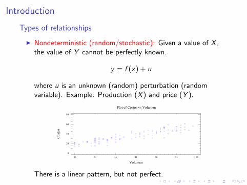
Introduction
Types of relationships
I Nondeterministic (random/stochastic): Given a value of X ,the value of Y cannot be perfectly known.
y = f (x) + u
where u is an unknown (random) perturbation (randomvariable). Example: Production (X ) and price (Y ).
Plot of Costos vs Volumen
Volumen
Costos
26 31 36 41 46 51 56
0
20
40
60
80
There is a linear pattern, but not perfect.

Introduction
Types of relationships
I Linear: When the function f (x) is linear,
f (x) = β0 + β1x
I If β1 > 0 there is a positive linear relationship.I If β1 < 0 there is a negative linear relationship.
Relación lineal positiva
X
Y
-2 -1 0 1 2
-6
-2
2
6
10
Relación lineal negativa
XY
-2 -1 0 1 2
-6
-2
2
6
10
The scatterplot is (American) football-shaped.
Introduction
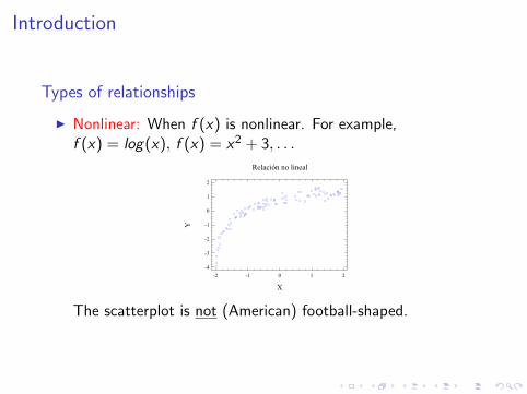
Types of relationships
I Nonlinear: When f (x) is nonlinear. For example,f (x) = log(x), f (x) = x2 + 3, . . .
Relación no lineal
X
Y
-2 -1 0 1 2
-4
-3
-2
-1
0
1
2
The scatterplot is not (American) football-shaped.

Introduction
Types of relationships
I Lack of relationship: When f (x) = 0.
Ausencia de relación
X
Y
-2 -1 0 1 2
-2,5
-1,5
-0,5
0,5
1,5
2,5

Measures of linear dependence
Covariance
The covariance is defined as
cov (x , y) =
n∑i=1
(xi − x) (yi − y)
n − 1=
n∑i=1
xiyi − n(x)(y)
n − 1
I If there is a positive linear relationship, cov > 0
I If there is a negative linear relationship, cov < 0
I If there is no relationship or the relationship is nonlinear,cov ≈ 0
Problem: Covariance depends on the units of X and Y .

Measures of linear dependence
Correlation coefficient
The correlation coefficient (unitless) is defined as
r(x ,y) = cor (x , y) =cov (x , y)
sxsy
where
s2x =
n∑i=1
(xi − x)2
n − 1and s2
y =
n∑i=1
(yi − y)2
n − 1
I -1≤ cor (x , y) ≤ 1
I cor (x , y) = cor (y , x)
I cor (ax + b, cy + d) = sign(a)sign(c)cor (x , y) for arbitrarynumbers a, b, c , d .

Simple linear regression model
The simple linear regression model assumes that
Yi = β0 + β1xi + ui
where
I Yi is the value of the dependent variable Y when the randomvariable X takes a specific value xi
I xi is the specific value of the random variable X
I ui is an error, a random variable that is assumed to be normalwith mean 0 and unknown variance σ2, ui ∼ N(0, σ2)
I β0 and β1 are the population coefficients:I β0 : population interceptI β1 : population slope
The (population) parameters that we need to estimate are: β0, β1
and σ2.

Simple linear regression modelOur objective is to find the estimators/estimates β0, β1 of β0, β1
in order to obtain the regression line:
y = β0 + β1x
which is the best fit to the data with a linear pattern. Example:
Let’s say that the regression line for the last example is
Price = −15.65 + 1.29 Production
Plot of Fitted Model
Volumen
Costos
26 31 36 41 46 51 56
0
20
40
60
80
Based on the regression line, we can estimate the price when
Production is 25 millions: Price = −15.65 + 1.29(25) = 16.6

Simple linear regression modelThe difference between the observed value of the response variableyi and its estimate yi is called a residual:
ei = yi − yi
Valor observado Dato (y)
Recta de regresiónestimada
Example (cont.): Clearly, if for a given year the production is 25millions, the price will not be exactly 16.6 mil euros. That smalldifference, the residual, in that case will be
ei = 18− 16.6 = 1.4

Simple linear regression model: model assumptionsI Linearity: The underlying relationship between X and Y is
linear,f (x) = β0 + β1x
I Homogeneity: The errors have mean zero,
E [ui ] = 0
I Homoscedasticity: The variance of the errors is constant,
Var(ui ) = σ2
I Independence: The errors are independent,
E [uiuj ] = 0
I Normality: The errors follow a normal distribution,
ui ∼ N(0, σ2)

Simple linear regression model: model assumptions
Linearity
The scaterplot should have an (American) football-shape, i.e., itshould show scatter around a straight line.
Plot of Fitted Model
Volumen
Costos
26 31 36 41 46 51 56
0
20
40
60
80
If not, the regression line is not an adequate model for the data.
Plot of Fitted Model
X
Y
-5 -3 -1 1 3 5
-6
4
14
24
34

Simple linear regerssion model: model assumptions
Homoscedasticity
The vertical spread around the line should roughly remainconstant.
Plot of Costos vs Volumen
40
60
80
Costos
26 31 36 41 46 51 56
Volumen
0
20
40
Costos
If that’s not the case, heteroscedasticity is present.

Simple linear regerssion model: model assumptions
Independence
I The observations should be independent.
I One observation doesn’t imply any information about another.
I In general, time series fail this assumption.
Normality
I A priori, we assume that the observations are normal.
2Regresión Lineal
Modelo general de regresión
Objetivo: Analizar la relación entre una o varias variables dependientes y un conjunto de factores independientes.
Tipos de relaciones:
- Relación no lineal
- Relación lineal
Regresión lineal simple
1 2 1 2( , ,..., | , ,..., )k lf Y Y Y X X X
3Regresión Lineal
Regresión simpleconsumo y peso de automóviles
Núm. Obs. Peso Consumo(i) kg litros/100 km
1 981 112 878 123 708 84 1138 115 1064 136 655 67 1273 148 1485 179 1366 1810 1351 1811 1635 2012 900 1013 888 714 766 915 981 1316 729 717 1034 1218 1384 1719 776 1220 835 1021 650 922 956 1223 688 824 716 725 608 726 802 1127 1578 1828 688 729 1461 1730 1556 15
0
5
10
15
20
25
500 700 900 1100 1300 1500 1700
Peso (Kg)
Con
sum
o (li
tros/
100
Km)
4Regresión Lineal
Modelo
ix
iyx10
osdesconocidparámetros:,, 210
),0(, 210 Nuuxy iiii
5Regresión Lineal
Hipótesis del modelo
Linealidadyi = 0+ 1xi + ui
Normalidadyi|xi N ( 0+ 1xi, 2)
HomocedasticidadVar [yi|xi] = 2
IndependenciaCov [yi, yk] = 0
21
0
Parámetros

(Ordinary) Least Square Estimators: LSE
In 1809 Gauss proposed the least squares method to obtain theestimators β0 and β1 that provide the best fit
yi = β0 + β1xi
The method is based on a criterion in which we minimize the sumof squares of the residuals, SSR, that is, the sum of squaredvertical distances between the observed yi and predicted yi values
n∑i=1
e2i =
n∑i=1
(yi − yi )2 =
n∑i=1
(yi −
(β0 + β1xi
))2
6Regresión Lineal
Modelo
),0(, 210 Nuuxy iiii
yi : Variable dependiente
xi : Variable independiente
ui : Parte aleatoria
0
7Regresión Lineal
Recta de regresión
y
ie
iy
x ix
8Regresión Lineal
Recta de regresión
xy 10ˆˆˆ
yPendiente
1ˆ
xy 10ˆˆ
x9Regresión Lineal
Residuos
ResiduoPrevistoValor
ˆˆ
ObservadoValor10 iii exy
iy
ii xy 10ˆˆˆ
ie
ix

Least Squares EstimatorsThe resulting estimators are
β1 =cov(x , y)
s2x
=
n∑i=1
(xi − x) (yi − y)
n∑i=1
(xi − x)2
β0 = y − β1x
6Regresión Lineal
Modelo
),0(, 210 Nuuxy iiii
yi : Variable dependiente
xi : Variable independiente
ui : Parte aleatoria
0
7Regresión Lineal
Recta de regresión
y
ie
iy
x ix
8Regresión Lineal
Recta de regresión
xy 10ˆˆˆ
yPendiente
1ˆ
xy 10ˆˆ
x9Regresión Lineal
Residuos
ResiduoPrevistoValor
ˆˆ
ObservadoValor10 iii exy
iy
ii xy 10ˆˆˆ
ie
ix
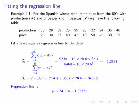
Fitting the regression line
Example 4.1. For the Spanish wheat production data from the 80’s withproduction (X ) and price per kilo in pesetas (Y ) we have the followingtable
production 30 28 32 25 25 25 22 24 35 40price 25 30 27 40 42 40 50 45 30 25
Fit a least squares regression line to the data.
β1 =
10∑i=1
xiyi − nx y
10∑i=1
x2i − nx2
=9734− 10× 28.6× 35.4
8468− 10× 28.62= −1.3537
β0 = y − β1x = 35.4 + 1.3537× 28.6 = 74.116
Regression line isy = 74.116− 1.3537x

Fitting the regression line in software

Estimating the error variance
To estimate the error variance, σ2, we can simply take theuncorrected sample variance,
σ2 =
n∑i=1
e2i
n
which is the so-called maximum likelihood estimator of σ2.However, this estimator is biased.
The unbiased estimator of σ2, is called the residual variance,
s2R =
n∑i=1
e2i
n − 2=
SSR
n − 2

Estimating the error variance
Exercise. 4.2. Find the residual variance for exercise 4.1.First, we find the residuals, ei , using the regression line
yi = 74.116− 1.3537xi
xi 30 28 32 25 25 25 22 24 35 40yi 25 30 27 40 42 40 50 45 30 25
yi = 74.116− 1.3537xi 33.5 36.21 30.79 40.27 40.27 40.27 44.33 41.62 26.73 19.96ei = yi − yi -8.50 -6.21 -3.79 -0.27 1.72 -0.27 5.66 3.37 3.26 5.03
The residual variance is then
s2R =
n∑i=1
e2i
n − 2=
207.92
8= 25.99
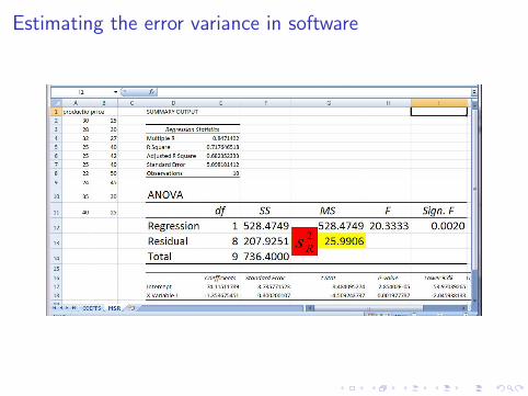
Estimating the error variance in software
Statistical inference in simple linear regression model
I Up to this point we only talked about point estimation.
I With confidence intervals for model parameters, we can obtaininformation about the estimation error.
I And tests of hypothesis will help us to decide if a givenparameter is statistically significant.
I In statistical inference, we begin with the distribution of theestimators.

Statistical inference of the slope
The estimator β1 follows a normal distribution because it is a linearcombination of normally distributed random variables
β1 =n∑
i=1
(xi − x)
(n − 1)s2X
Yi =n∑
i=1
wiYi
where Yi = β0 + β1xi + ui , and satisfies Yi ∼ N(β0 + β1xi , σ
2).
In addition, β1 is an unbiased estimator of β1,
E[β1
]=
n∑i=1
(xi − x)
(n − 1)s2X
E [Yi ] = β1
whose variance is,
Var[β1
]=
n∑i=1
((xi − x)
(n − 1)s2X
)2
Var [Yi ] =σ2
(n − 1)s2X
Thus,
β1 ∼ N
(β1,
σ2
(n − 1)s2X
)

Confidence interval for the slopeWe wish to obtain a (1− α) confidence interval for β1. Since σ2 isunknown, we estimate it using s2
R . The corresponding theoreticalresult, when the error variance is unknown is then
β1 − β1√s2R
(n − 1)s2X
∼ tn−2
based on which we obtain (1− α) confidence interval for β1:
β1 ± tn−2,α/2
√s2R
(n − 1)s2X
The length of the interval decreases if:
I The sample size increases.
I The variance of xi increases.
I The residual variance decreases.

Hypothesis testing for the slope
In a similar manner, we construct a hypothesis test for β1. In particular, if the truevalue of β1 is zero, this means that the variable Y does not depend on X in a linearfashion. Thus, we are mainly interested in a two-sided test:
H0 : β1 = 0
H1 : β1 6= 0
The rejection region is :
RRα =
8>>>><>>>>:t :
˛˛˛
tz }| {β1q
s2R/((n − 1)s2
X )
˛˛˛ > tn−2,α/2
9>>>>=>>>>;Equivalently, if 0 is outside a (1− α) confidence interval for β1, we reject the null at αsignificance level.The p-value is:
p-value = 2 Pr
0B@Tn−2 >
˛˛ β1q
s2R/((n − 1)s2
X )
˛˛1CA

Inference for the slopeExercise 4.3
1. Find a 95% CI for the slope of the (population) regression modelfrom Example 4.1.
2. Test the hypothesis that the price of wheat depends linearly on theproduction at a 0.05 significance level.
1. Since tn−2,α/2 = t8,0.025 = 2.306
−2.306 ≤ −1.3537− β1√25.99
9×32.04
≤ 2.306
−2.046 ≤ β1 ≤ −0.661
2. Since the interval (with the same α) doesn’t contain 0, we reject thenull β1 = 0 at 0.05 level. Also, the (observed) test statistic is
t =β1√
s2R/ (n − 1) s2
X
=−1.3537√
25.999×32.04
= −4.509.
Thus, we have p-value = 2 Pr(|T8| > | − 4.509|) = 0.002

Inference for β1 in software

Statistical inference for the intercept
The estimator β0 follows a normal distribution because it is a linearcombination of normal random variables,
β0 =n∑
i=1
(1
n− xwi
)Yi
where wi = (xi − x) /ns2X and Yi = β0 + β1xi + ui , which satisfies
Yi ∼ N(β0 + β1xi , σ
2). Additionally, β0 is an unbiased estimator
of β0,
E[β0
]=
n∑i=1
(1
n− xwi
)E [Yi ] = β0
whose variance is,
Var[β0
]=
n∑i=1
(1
n− xwi
)2
Var [Yi ] = σ2
(1
n+
x2
(n − 1)s2X
).
Thus,
β0 ∼ N
(β0, σ
2
(1
n+
x2
(n − 1)s2X
))

Confidence interval for the intercept
We wish to find a (1− α) confidence interval for β0. Since σ2 isunknown, we estimate it with s2
R as before. We obtain:
β0 − β0√s2R
(1
n+
x2
(n − 1)s2X
) ∼ tn−2
which yields the following confidence interval for β0:
β0 ± tn−2,α/2
√s2R
(1n + x2
(n−1)s2X
)The length of the interval decreases if:
I The sample size increases.
I Variance of xi increases.
I The residual variance decreases.
I The mean of xi decreases.

Hypothesis test for the intercept
Based on the distribution of the estimator, we can carry out the test of hypothesis. Inparticular, if the true value of β0 is 0, it means that the population regression line goesthrough the origin. For this case we would test:
H0 : β0 = 0
H1 : β0 6= 0
The rejection region is:
RRα =
8>>>><>>>>:t :
˛˛˛
tz }| {β0s
s2R
„1n
+ x2
(n−1)s2X
«˛˛˛ > tn−2,α/2
9>>>>=>>>>;Equivalently, if 0 is outside the (1− α) confidence interval for β0 we reject the null.The p-value is
p-value = 2 Pr
0BBBB@Tn−2 >
˛˛˛
β0ss2R
„1n
+ x2
(n−1)s2X
«˛˛˛
1CCCCA

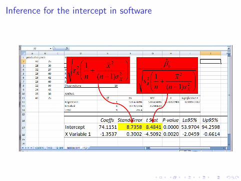
Inference for the interceptExercise 4.4
1. Find a 95% CI for the intercept of the population regression line ofExercise 4.1.
2. Test the hypothesis that the population regression line intersects theorigin at a 0.05 significance level.
1. The quantile is tn−2,α/2 = t8,0.025 = 2.306 so
−2.306 ≤ 74.1151− β0√25.99
(1
10 + 28.62
9×32.04
) ≤ 2.306⇔ 53.969 ≤ β0 ≤ 94.261
2. Since the interval (with the same α) doesn’t contain 0, we reject thenull hypothesis that β0 = 0. Also, the (observed) test statistic is
t =
t︷ ︸︸ ︷β0√
s2R
(1n + x2
(n−1)s2X
) =74.1151√
25.99(
110 + 28.62
9×32.04
) = 8.484
Thus, we have: p-value = 2 Pr(|T8| > |8.483|) = 0.000 .
Inference for the intercept in software

Inference for the error variance
We have:(n − 2) s2
R
σ2∼ χ2
n−2
Which means that :
I The (1− α) confidence interval for σ2 is:
(n − 2) s2R
χ2n−2,α/2
≤ σ2 ≤(n − 2) s2
R
χ2n−2,1−α/2
I Which can be used to solve the test:
H0 : σ2 = σ20
H1 : σ2 6= σ20

Average and individual predictionsWe consider two situations:
1. We wish to estimate/predict the average value of Y for agiven X = x0.
2. We wish to estimate/predict the actual value of Y for a givenX = x0.
For example in Ex. 4.1
1. What would be the average wheat price for all years in whichthe production was 30?
2. If in a given year, the production was 30, what would be thecorresponding price of wheat?
In both cases:
y0 = β0 + β1x0
= y + β1 (x0 − x)
But the estimation errors are different.

Estimating/predicting the average value
Remember that:
Var(Y0
)= Var
(Y)
+ (x0 − x)2 Var(β1
)= σ2
(1
n+
(x0 − x)2
(n − 1) s2X
)
The confidence interval for the mean prediction E [Y0|X = x0] is:
Y0 ± tn−2,α/2
√√√√s2R
(1
n+
(x0 − x)2
(n − 1) s2X
)

Estimating/predicting the actual value
The variance for the prediction of the actual value is the meansquared error:
E
[(Y0 − Y0
)2]
= Var (Y0) + Var(Y0
)= σ2
(1 +
1
n+
(x0 − x)2
(n − 1) s2X
)
And thus the confidence interval for the actual value Y0 is:
Y0 ± tn−2,α/2
√√√√s2R
(1 +
1
n+
(x0 − x)2
(n − 1) s2X
)
The size of this interval is bigger than that for the averageprediction.

Estimating/predicting the average and actual values
In red: confidence intervals for the prediction of average value.In pink: confidence intervals for the prediction of actual value.
Plot of Fitted Model
22 25 28 31 34 37 40
Produccion en kg.
25
30
35
40
45
50
Precio en ptas.
Regression line: R-squared and variability decomposition
I Coefficient of determination, R-squared is used to assess thegoodness-of-fit of the model. It is defined as
R2 = r2(x,y) ∈ [0, 1]
I R2 tells us what percentage of the sample variability in the yvariable is explained by the model, that is, by its linear dependenceon x
I Values close to 100% indicate that the regression model is a goodfit to the data (less than 60%, not so good)
I Variability decomposition and R2: The Total Sum of Squares∑i (yi − y)2 can be decomposed into the Residual Sum of Squares∑i (yi − y)2 + the Model Sum of Squares
∑i (y − y)2
SST = SSR + SSM
and we have R2 = 1− SSRSST = SSM
SST

Regression line: R-squared and variability decomposition
From Wikipedia:

ANOVA table
ANOVA (Analysis of Variance) table for the simple linearregression model
Source of variability SS DF Mean F ratio
Model SSM 1 SSM/1 SSM/s2R
Residuals/errors SSR n − 2 SSR/(n − 2) = s2R
Total SST n − 1
Note that the value of the F statistic is the square of that for the tstatistic in the simple regression significance test.
Recommended