Essex EC248-2-SPLecture 5
The Demand for Money and Monetary Theory
Alexander Mihailov, 13/02/06

© 2004 Pearson Addison-Wesley. All rights reserved 5-2
Plan of Talk
• Introduction1. Theories on the Demand for Money2. Money in IS-LM and AD-AS Analysis3. Money and Inflation4. Money and Output • Wrap-up

© 2004 Pearson Addison-Wesley. All rights reserved 5-3
Aims and Learning Outcomes
• Aims– Understand what determines money demand– Discuss the role of money and policy in the economy
• Learning outcomes– Compare alternative theories of money demand– Analyse effects of money in IS-LM and AD-AS models– Comment the link between money and inflation– Characterise the real effects of money

5-4
Quantity Theory of MoneyP × Y
Velocity V ≡ (definition)M
Equation of Exchange M × V ≡ P × Y(identity)Quantity Theory of Money1. Irving Fisher’s (1911) view: V is fairly constant2. Equation of exchange no longer identity, but theory3. Nominal income, PY, determined by M4. Classicals assume Y fairly constant5. P determined by M

© 2004 Pearson Addison-Wesley. All rights reserved 5-5
Change in Velocity fromYear to Year: US Data, 1915–2002

© 2004 Pearson Addison-Wesley. All rights reserved 5-6
Cambridge Approach and Keynes (1936)
Cambridge approach: Is velocity constant?1. Classicals thought V constant because they did not have good data2. Great Depression => economists realised velocity was far from constant
Keynes: 3 motives to hold money1. Transactions motive—related to Y2. Precautionary motive—related to Y3. Speculative motive
A. related to W and YB. negatively related to i
Liquidity PreferenceMd
= f(i, Y)P – +

© 2004 Pearson Addison-Wesley. All rights reserved 5-7
Keynes’s Liquidity Preference Theory
Implication: Velocity not constant
P 1=
Md f(i,Y)
Multiply both sides by Y and substitute in M = Md
PY YV= =
M f(i,Y)
1. i ↑, f(i,Y) ↓, V ↑2. Change in expectations of future i, change f(i,Y) and V changes
© 2004 Pearson Addison-Wesley. All rights reserved 5-8
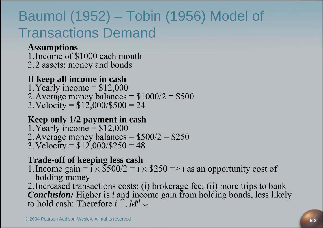
Baumol (1952) – Tobin (1956) Model of Transactions Demand
Assumptions1.Income of $1000 each month2.2 assets: money and bondsIf keep all income in cash1.Yearly income = $12,0002.Average money balances = $1000/2 = $5003.Velocity = $12,000/$500 = 24Keep only 1/2 payment in cash1.Yearly income = $12,0002.Average money balances = $500/2 = $2503.Velocity = $12,000/$250 = 48Trade-off of keeping less cash1.Income gain = i × $500/2 = i × $250 => i as an opportunity cost of
holding money2.Increased transactions costs: (i) brokerage fee; (ii) more trips to bankConclusion: Higher is i and income gain from holding bonds, less likely to hold cash: Therefore i ↑, Md ↓

© 2004 Pearson Addison-Wesley. All rights reserved 5-9
Cash Balance in Baumol-Tobin Model

5-10
Precautionary and Speculative Md
Precautionary DemandSimilar trade-off to Baumol-Tobin framework
1. Benefits of precautionary balances2. Opportunity cost of interest foregone
Conclusion:i ↑, opportunity cost ↑, hold less precautionary balances, Md ↓
Speculative DemandProblems with Keynes’s framework:
Hold all bonds or all money: no diversification
Tobin (1958) Model1. People want high Re, but low risk2. As i ↑, hold more bonds and less M, but still diversify and hold M
Problem with Tobin model: No speculative demand because T-bills have no risk (like money) but have higher return
5-11
Friedman’s (1956) Modern Quantity Theory
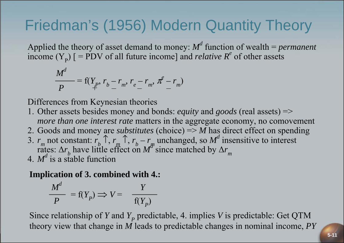
Implication of 3. combined with 4.:Md Y
= f(YP) ⇒ V =P f(YP)
Since relationship of Y and YP predictable, 4. implies V is predictable: Get QTM theory view that change in M leads to predictable changes in nominal income, PY
Applied the theory of asset demand to money: Md function of wealth = permanentincome (YP) [ = PDV of all future income] and relative Re of other assets
Md
= f(YP, rb – rm, re – rm, πe – rm)P + – – –
Differences from Keynesian theories1. Other assets besides money and bonds: equity and goods (real assets) =>
more than one interest rate matters in the aggregate economy, no comovement2. Goods and money are substitutes (choice) => M has direct effect on spending3. rm not constant: rb ↑, rm ↑, rb – rm unchanged, so Md insensitive to interest
rates: Δrb have little effect on Md since matched by Δrm4. Md is a stable function
© 2004 Pearson Addison-Wesley. All rights reserved 5-12
Empirical Evidence on Money Demand
Interest Rate Sensitivity of Money DemandIs sensitive, but no liquidity trap
Stability of Money Demand1. M1 demand stable till 1973, unstable after2. Most likely source of instability is financial
innovation3. Cast doubts on money targets
5-13
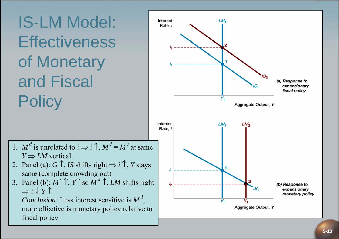
IS-LM Model: Effectiveness of Monetary and Fiscal Policy
1. M d is unrelated to i ⇒ i ↑, M d = M s at same Y ⇒ LM vertical
2. Panel (a): G ↑, IS shifts right ⇒ i ↑, Y stays same (complete crowding out)
3. Panel (b): M s ↑, Y↑ so M d ↑, LM shifts right ⇒ i ↓ Y ↑Conclusion: Less interest sensitive is M d, more effective is monetary policy relative to fiscal policy

5-14
AD-AS Analysis: Monetarist View of AD
P × Y 1 × 2000V= = = 2
M 1000Modern Quantity Theory of Money (Friedman, 1956)M × V = P × YImplication: M determines P × Y if V predictable and unrelated to ΔMDeriving AD CurveP=1, M = 1000, V = 2 ⇒ P × Y = 2000 (Point B below)
Point A: P = 2 Y = 1000 PY = 2 × 1000 = 2000Point B: P = 1 Y = 2000 PY = 1 × 2000 = 2000Point C: P = 0.5 Y = 4000 PY = 0.5 × 4000 = 2000Conclusion: P ↓, Y ↑, downward sloping AD2 Key Differences w.r.t. Keynesians (see also next slide):
– Shift in AD Curve: one primary source, ΔM (e.g., if M = 2000 above)M ↑ <=> P×Y ↑, i.e., AD shifts right (at any given P)
– Crowding out: complete (see next slide)
5-15
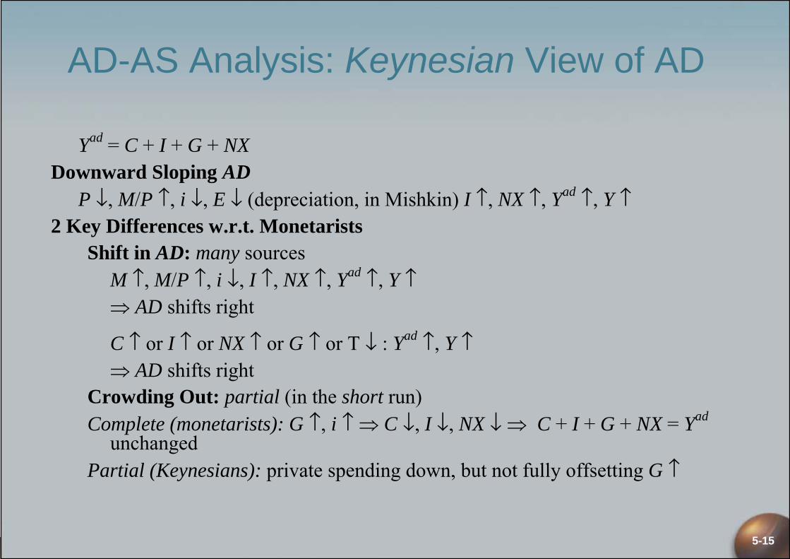
AD-AS Analysis: Keynesian View of AD
Yad = C + I + G + NXDownward Sloping AD
P ↓, M/P ↑, i ↓, E ↓ (depreciation, in Mishkin) I ↑, NX ↑, Yad ↑, Y ↑2 Key Differences w.r.t. Monetarists
Shift in AD: many sourcesM ↑, M/P ↑, i ↓, I ↑, NX ↑, Yad ↑, Y ↑⇒ AD shifts right
C ↑ or I ↑ or NX ↑ or G ↑ or T ↓ : Yad ↑, Y ↑⇒ AD shifts right
Crowding Out: partial (in the short run)Complete (monetarists): G ↑, i ↑ ⇒ C ↓, I ↓, NX ↓ ⇒ C + I + G + NX = Yad
unchangedPartial (Keynesians): private spending down, but not fully offsetting G ↑

5-16
Money and Inflation: The Evidence
“Inflation is always and everywhere a monetary phenomenon”(M. Friedman)
EvidenceIn every case when π high for sustained period, M growth is high
Examples:1. Latin American inflations2. German Hyperinflation, 1921–1923Controlled experiment, particularly after 1923 French invasion of Ruhr—government prints money to pay strikers, π > 1 million %
Meaning of “inflation”Friedman’s statement uses definition of π as continuing, rapidly rising price level: only then does evidence support it!

© 2004 Pearson Addison-Wesley. All rights reserved 5-17
German Hyperinflation: 1921–1923

5-18
Monetarist and Keynesian Views on πMonetarist View
Only source of AD shifts and π can be Ms growth
Keynesian ViewAllows for other sources of AD shifts, but comes to same conclusion that only source of sustained high π is Ms growth
Lags in Shifting AD1. Data lag2. Recognition lag3. Legislative lag4. Implementation lag5. Effectiveness lag
Case for Activist PolicyIf self-correcting mechanism is slow (U > Un for long time)
Case for Nonactivist PolicyIf self-correcting mechanism is fast

© 2004 Pearson Addison-Wesley. All rights reserved 5-19
Lucas (1976) Critique
Lucas challenges usefulness of econometric models for policy evaluation1. Critique follows from RE implication that change in way variable moves,
changes way expectations are formed2. Policy change, changes relationship between expectations and past behavior3. Estimated relationships in econometric model change4. Therefore, can’t be used to evaluate change in policy
Example: Evaluate effect on long rate from Fed policy raising short-term i permanently, if in past changes in i quickly reversed (were temporary)
1. Estimated term structure relationship indicates only small change in long rate2. Once realize short i ↑ permanently, average future short rates ↑ a lot, long
rate ↑ a lot3. Another implication of Lucas analysis: expectations about policy influence
response to policy

© 2004 Pearson Addison-Wesley. All rights reserved 5-20
New (Neo)Classical Model
Assumptions:1. Rational expectations2. Wages and prices completely flexible with respect to expected
inflation: adjust immediately and fully to changes in the expected price level
Implications:1. Policy ineffectiveness proposition: anticipated policy has no
effect on business cycle2. Effects of (unanticipated) policy are uncertain because they
depend on expectations3. No beneficial effect from activist policy: supports nonactivism

© 2004 Pearson Addison-Wesley. All rights reserved 5-21
New Keynesian (or NNS) Model
Assumptions:1. Rational expectations2. Wages and prices display rigidity: do not adjust immediately
(and fully) to changes in the expected price level
Implications:1. Unanticipated policy has larger effect on Y than anticipated
policy2. But policy ineffectiveness does not hold:
Anticipated policy does affect Y!3. Does not rule out beneficial effect from activist policy4. However, effects of policy are affected by expectations:
designing policy is tough
© 2004 Pearson Addison-Wesley. All rights reserved 5-22
Concluding Wrap-Up
• What have we learnt?– How alternative theories of money demand differ– What is the role of money in IS-LM and AD-AS models– Why inflation is ultimately a monetary phenomenon– What are the effects of money and policy on output
• Where we go next: to the formulation and implementation of monetary policy by central banks
Recommended