Essays on Financial Econometrics:
Variance and Covariance
Estimation Using Price Durations
Xiaolu Zhao
Thesis submitted in fulfilment of the requirements
for the degree of Doctor of Philosophy in Finance
Department of Accounting and Finance
Lancaster University Management School
May 2017

Declaration
I hereby declare that this thesis is my own work and has not been submitted for
the award of a higher degree elsewhere. This thesis contains no material previously
published or written by any other person except where references have been made
in the thesis.
Xiaolu Zhao
May 2017
1

Acknowledgement
I would like to express my gratitude towards my supervisors, Professor Stephen Tay-
lor and Professor Ingmar Nolte, for their guidance and support.
I want to thank my friends for their warmth and friendship.
I dedicate this thesis to my parents.
2
Contents
List of Tables 7
List of Figures 10
Introduction 15
1 Volatility estimation and forecasting literature 16
1.1 Introduction . . . . . . . . . . . . . . . . . . . . . . . . . . . . . . . . 17
1.2 Parametric volatility modelling . . . . . . . . . . . . . . . . . . . . . 18
1.2.1 Continuous-time models . . . . . . . . . . . . . . . . . . . . . 18
1.2.2 Discrete-time models . . . . . . . . . . . . . . . . . . . . . . . 19
1.3 Nonparametric realised volatility estimation using high-frequency data 21
1.4 Popular nonparametric volatility estimators . . . . . . . . . . . . . . 23
1.4.1 General setup . . . . . . . . . . . . . . . . . . . . . . . . . . . 24
1.4.2 Two-scaled realized volatility . . . . . . . . . . . . . . . . . . 26
1.4.3 Flat-top realized kernel . . . . . . . . . . . . . . . . . . . . . . 28
1.4.4 The OLS framework for jointly estimating return and noise
variances . . . . . . . . . . . . . . . . . . . . . . . . . . . . . . 29
3
1.4.5 Realized Bipower variation . . . . . . . . . . . . . . . . . . . . 31
1.4.6 Bipower downward semi-variance . . . . . . . . . . . . . . . . 33
1.4.7 Model-free option-implied volatility estimator and implemen-
tation . . . . . . . . . . . . . . . . . . . . . . . . . . . . . . . 35
1.5 Volatility forecasting . . . . . . . . . . . . . . . . . . . . . . . . . . . 37
1.6 Remarks . . . . . . . . . . . . . . . . . . . . . . . . . . . . . . . . . . 40
2 More accurate volatility estimation and forecasts using price dura-
tions 41
2.1 Introduction . . . . . . . . . . . . . . . . . . . . . . . . . . . . . . . . 43
2.2 Theoretical foundation . . . . . . . . . . . . . . . . . . . . . . . . . . 48
2.2.1 Duration based integrated variance estimators: pure diffusion
setting . . . . . . . . . . . . . . . . . . . . . . . . . . . . . . . 49
2.2.2 Market microstructure noise . . . . . . . . . . . . . . . . . . . 54
2.3 Data properties . . . . . . . . . . . . . . . . . . . . . . . . . . . . . . 57
2.4 Simulation results . . . . . . . . . . . . . . . . . . . . . . . . . . . . . 60
2.4.1 Time-discretization . . . . . . . . . . . . . . . . . . . . . . . . 60
2.4.2 Bid/ask spread and time-discretization . . . . . . . . . . . . . 62
2.4.3 Bias versus efficiency: the preferred threshold value . . . . . . 63
2.4.4 Price-discretization . . . . . . . . . . . . . . . . . . . . . . . . 64
2.4.5 Jumps . . . . . . . . . . . . . . . . . . . . . . . . . . . . . . . 65
2.4.6 Simulation comparison of different estimators . . . . . . . . . 66
2.5 Empirical analysis . . . . . . . . . . . . . . . . . . . . . . . . . . . . . 67
2.5.1 Parametric duration based variance estimator . . . . . . . . . 67
4
2.5.2 The preferred threshold value . . . . . . . . . . . . . . . . . . 69
2.6 Volatility forecasts evaluation . . . . . . . . . . . . . . . . . . . . . . 71
2.6.1 Individual forecasts . . . . . . . . . . . . . . . . . . . . . . . . 72
2.6.2 Combinations of forecasts . . . . . . . . . . . . . . . . . . . . 76
2.7 Conclusion . . . . . . . . . . . . . . . . . . . . . . . . . . . . . . . . . 77
2.8 Appendix: Comparison of density functions . . . . . . . . . . . . . . 89
3 High-frequency covariance matrix estimation using price durations 99
3.1 Introduction . . . . . . . . . . . . . . . . . . . . . . . . . . . . . . . . 101
3.2 Theoretical foundation . . . . . . . . . . . . . . . . . . . . . . . . . . 104
3.2.1 Three approaches . . . . . . . . . . . . . . . . . . . . . . . . . 104
3.2.2 NPDV . . . . . . . . . . . . . . . . . . . . . . . . . . . . . . . 105
3.3 Data properties . . . . . . . . . . . . . . . . . . . . . . . . . . . . . . 108
3.4 Simulation results . . . . . . . . . . . . . . . . . . . . . . . . . . . . . 111
3.4.1 Simulation on one pair of assets . . . . . . . . . . . . . . . . . 112
3.4.2 Simulation of the covariance matrix . . . . . . . . . . . . . . . 118
3.5 Empirical study . . . . . . . . . . . . . . . . . . . . . . . . . . . . . . 120
3.5.1 Comparison among candidate covariance matrix estimators . . 120
3.5.2 A portfolio allocation problem . . . . . . . . . . . . . . . . . . 123
3.6 Conclusion . . . . . . . . . . . . . . . . . . . . . . . . . . . . . . . . . 134
3.7 Appendix . . . . . . . . . . . . . . . . . . . . . . . . . . . . . . . . . 156
3.7.1 Correlated Bernoulli processes . . . . . . . . . . . . . . . . . . 156
3.7.2 Empirical supplements . . . . . . . . . . . . . . . . . . . . . . 156
5

Concluding remarks 162
Bibliography 163
6
List of Tables
2.1 Descriptive statistics for 20 DJIA stocks . . . . . . . . . . . . . . . . 79
2.2 Simulation comparison with other estimators . . . . . . . . . . . . . . 83
2.3 Illustrative parameter values and tests results: AXP, year 2008, with
threshold value equal to 12 ticks . . . . . . . . . . . . . . . . . . . . . 84
2.4 Bid/ask spread level groups, AXP . . . . . . . . . . . . . . . . . . . . 85
2.5 Diebold-Mariano test summary results, individual forecasts, 10 pairs,
3 horizons, 20 firms . . . . . . . . . . . . . . . . . . . . . . . . . . . . 86
2.6 Diebold-Mariano test summary results, combination forecasts, 7 pairs,
3 horizons, 20 firms . . . . . . . . . . . . . . . . . . . . . . . . . . . . 88
2.7 LR test results, HD . . . . . . . . . . . . . . . . . . . . . . . . . . . . 90
2.8 LB test results for 30 and 50 lags, HD . . . . . . . . . . . . . . . . . 90
2.9 DF test results, HD . . . . . . . . . . . . . . . . . . . . . . . . . . . . 91
2.10 LR test results, MCD . . . . . . . . . . . . . . . . . . . . . . . . . . . 91
2.11 LB test results for 30 and 50 lags, MCD . . . . . . . . . . . . . . . . 92
2.12 DF test results, MCD . . . . . . . . . . . . . . . . . . . . . . . . . . . 92
2.13 LR test results, AXP . . . . . . . . . . . . . . . . . . . . . . . . . . . 93
2.14 LB test results for 30 and 50 lags, AXP . . . . . . . . . . . . . . . . . 93
7
2.15 DF test results, AXP . . . . . . . . . . . . . . . . . . . . . . . . . . . 94
2.16 LR test results, IBM . . . . . . . . . . . . . . . . . . . . . . . . . . . 95
2.17 LB test results for 30 and 50 lags, IBM . . . . . . . . . . . . . . . . . 96
2.18 DF test results, IBM . . . . . . . . . . . . . . . . . . . . . . . . . . . 97
2.19 Diagnostic test results for 20 DJIA stocks . . . . . . . . . . . . . . . 98
3.1 Descriptive statistics for 19 DJIA stocks . . . . . . . . . . . . . . . . 135
3.2 Correlations of returns and trade arrivals . . . . . . . . . . . . . . . . 136
3.3 Comparison of the three duration-based covariance methods with
other covariance estimators . . . . . . . . . . . . . . . . . . . . . . . . 137
3.4 Comparison of different covariance matrix estimates for 19 simulated
stocks . . . . . . . . . . . . . . . . . . . . . . . . . . . . . . . . . . . 138
3.5 5min & 30min realised covariance matrix . . . . . . . . . . . . . . . . 139
3.6 COV1 & COV2 vs. 5min realised covariance estimators . . . . . . . . 139
3.7 RK & TS vs. 5min realised covariance estimators . . . . . . . . . . . 140
3.8 COV1 & COV2 vs. 30min realised covariance estimators . . . . . . . . 140
3.9 RK & TS vs. 30min realised covariance estimators . . . . . . . . . . . 141
3.10 Open-to-close covariance matrix . . . . . . . . . . . . . . . . . . . . . 141
3.11 COV1 & COV2 vs. OtoC covariance estimators . . . . . . . . . . . . . 142
3.12 RK & TS vs. OtoC covariance estimators . . . . . . . . . . . . . . . 142
3.13 Difference comparison summary . . . . . . . . . . . . . . . . . . . . . 145
3.14 Summary statistics: all estimators . . . . . . . . . . . . . . . . . . . . 149
3.15 Correlations among estimators . . . . . . . . . . . . . . . . . . . . . . 149
8
3.16 Equal-weight, risk-parity, and GMV portfolio variances under eigen-
value cleaning and shrinkage techniques . . . . . . . . . . . . . . . . 151
3.17 GMV results with the coarse shrinkage method for different allocation
targets . . . . . . . . . . . . . . . . . . . . . . . . . . . . . . . . . . . 151
3.18 GMV results with coarse shrinkage method when λ = 0.75 for all
estimators . . . . . . . . . . . . . . . . . . . . . . . . . . . . . . . . . 153
3.19 GMV results with coarse shrinkage method under different ηu . . . . 153
3.20 GMV results combining coarse and fine shrinkage methods . . . . . . 155
3.21 GMV results under the fine shrinkage method . . . . . . . . . . . . . 160
9
List of Figures
2.1 Bid/ask spread, trade duration and volatility for American Express
(AXP) . . . . . . . . . . . . . . . . . . . . . . . . . . . . . . . . . . . 80
2.2 The time-discretization noise . . . . . . . . . . . . . . . . . . . . . . . 80
2.3 Combined effect of spread and time-discretization: bias . . . . . . . . 81
2.4 Standard deviations of the NP variance estimator . . . . . . . . . . . 81
2.5 Plot of MSE as a function of the threshold value . . . . . . . . . . . . 82
2.6 Including price-discretization noise . . . . . . . . . . . . . . . . . . . 82
2.7 100 small jumps a day . . . . . . . . . . . . . . . . . . . . . . . . . . 83
2.8 Daily NP estimates for AXP: October 2008 . . . . . . . . . . . . . . 84
2.9 AXP: relationship between variance, threshold and bid/ask spread level 85
2.10 RMSEs, individual forecast, one-day ahead . . . . . . . . . . . . . . . 85
2.11 RMSEs, individual forecast, one-week ahead . . . . . . . . . . . . . . 86
2.12 RMSEs, individual forecast, one-month ahead . . . . . . . . . . . . . 86
2.13 RMSEs, combination forecast, one-day ahead . . . . . . . . . . . . . . 87
2.14 RMSEs, combination forecast, one-week ahead . . . . . . . . . . . . . 87
2.15 RMSEs, combination forecast, one-month ahead . . . . . . . . . . . . 87
10
3.1 Average correlation between trade arrivals . . . . . . . . . . . . . . . 143
3.2 Identical trade arrivals, ρarr = 1 . . . . . . . . . . . . . . . . . . . . . 143
3.3 Independent trade arrivals, ρarr = 0 . . . . . . . . . . . . . . . . . . . 144
3.4 Correlated trade arrivals, ρarr = 0.4 . . . . . . . . . . . . . . . . . . . 144
3.5 Correlated arrivals with spread . . . . . . . . . . . . . . . . . . . . . 145
3.6 Bias: scenario 1 . . . . . . . . . . . . . . . . . . . . . . . . . . . . . . 146
3.7 Bias: scenario 2 . . . . . . . . . . . . . . . . . . . . . . . . . . . . . . 146
3.8 Bias: scenario 3 . . . . . . . . . . . . . . . . . . . . . . . . . . . . . . 146
3.9 STD: scenario 1 . . . . . . . . . . . . . . . . . . . . . . . . . . . . . . 147
3.10 STD: scenario 2 . . . . . . . . . . . . . . . . . . . . . . . . . . . . . . 147
3.11 STD: scenario 3 . . . . . . . . . . . . . . . . . . . . . . . . . . . . . . 147
3.12 RMSE: scenario 1 . . . . . . . . . . . . . . . . . . . . . . . . . . . . . 148
3.13 RMSE: scenario 2 . . . . . . . . . . . . . . . . . . . . . . . . . . . . . 148
3.14 RMSE: scenario 3 . . . . . . . . . . . . . . . . . . . . . . . . . . . . . 148
3.15 Eigenvalue ratios of duration based covariance matrix . . . . . . . . . 150
3.16 Eigenvalue ratios of RK covariance matrix . . . . . . . . . . . . . . . 150
3.17 Eigenvalue ratios of TS covariance matrix . . . . . . . . . . . . . . . 150
3.18 Average weights for 19 assets . . . . . . . . . . . . . . . . . . . . . . 152
3.19 STD of weights for 19 assets . . . . . . . . . . . . . . . . . . . . . . . 152
3.20 ξ over time under the fine shrinkage method, ηu = 100 . . . . . . . . 154
3.21 ξ over time under the fine shrinkage method, ηu = 190 . . . . . . . . 154
3.22 Eigenvalue ratios, COV , coarse shrinkage . . . . . . . . . . . . . . . . 157
3.23 Eigenvalue ratios, RK, coarse shrinkage . . . . . . . . . . . . . . . . . 157
11
3.24 Eigenvalue ratios, TS, coarse shrinkage . . . . . . . . . . . . . . . . . 157
3.25 Eigenvalue ratios, sub5min, coarse shrinkage . . . . . . . . . . . . . . 158
3.26 η, COV , coarse shrinkage . . . . . . . . . . . . . . . . . . . . . . . . 158
3.27 η, RK, coarse shrinkage . . . . . . . . . . . . . . . . . . . . . . . . . . 159
3.28 η, TS, coarse shrinkage . . . . . . . . . . . . . . . . . . . . . . . . . . 159
3.29 η, sub5min, coarse shrinkage . . . . . . . . . . . . . . . . . . . . . . . 159
3.30 η, TS, raw . . . . . . . . . . . . . . . . . . . . . . . . . . . . . . . . . 160
12
Introduction
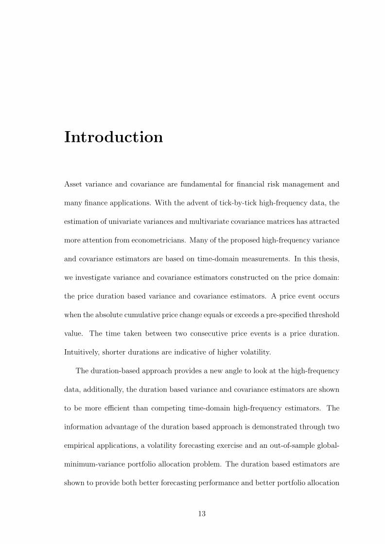
Asset variance and covariance are fundamental for financial risk management and
many finance applications. With the advent of tick-by-tick high-frequency data, the
estimation of univariate variances and multivariate covariance matrices has attracted
more attention from econometricians. Many of the proposed high-frequency variance
and covariance estimators are based on time-domain measurements. In this thesis,
we investigate variance and covariance estimators constructed on the price domain:
the price duration based variance and covariance estimators. A price event occurs
when the absolute cumulative price change equals or exceeds a pre-specified threshold
value. The time taken between two consecutive price events is a price duration.
Intuitively, shorter durations are indicative of higher volatility.
The duration-based approach provides a new angle to look at the high-frequency
data, additionally, the duration based variance and covariance estimators are shown
to be more efficient than competing time-domain high-frequency estimators. The
information advantage of the duration based approach is demonstrated through two
empirical applications, a volatility forecasting exercise and an out-of-sample global-
minimum-variance portfolio allocation problem. The duration based estimators are
shown to provide both better forecasting performance and better portfolio allocation
13
results. The paper in Chapter 2 is under the first round Revise&Resubmit to the
Journal of Business & Economic Statistics.
In Chapter 2, we discuss the estimation of univariate variance using price dura-
tions. Variance estimation using high-frequency data needs to take into account the
effect of market microstructure (MMS) noise, including discrete transaction times,
discrete price levels, and bid/ask spreads, as well as price jumps. The price duration
estimator has a built-in feature to be robust to large price jumps, while its robust-
ness against the MMS noise is achieved through a careful selection of the threshold
value that defines a price event. We discuss the selection of this optimal threshold
value through both simulation and empirical evidence.
We devise both a non-parametric and a parametric estimator. For the estima-
tion of integrated variance at a daily frequency, the non-parametric duration based
variance estimator suffices, while the parametric estimator additionally provides us
with an instantaneous variance estimator.
As an empirical application to 20 DJIA stocks, we compare the volatility fore-
casting performance of three classes of volatility estimators, including the realized
volatility, the option implied volatility, and the price duration based volatility es-
timators, on one-day, one-week, and one-month horizons. Forecasting comparisons
among individual estimators, as well as in a combination setup, are considered. The
duration based estimators, especially the parametric price duration volatility esti-
mator, are found to provide more accurate out-of-sample forecasts.
In Chapter 3, we introduce a covariance matrix estimator using price durations.
In the multivariate setting, there is the additional issue of nonsynchronous trade
14
arrival times when estimating a high-dimensional variance-covariance matrix using
tick-by-tick transaction data. Through simulation, we assess the effects of the last-
tick time-synchronization method and MMS noise on the duration based covariance
estimator, and compare its accuracy and efficiency with other candidate covariance
estimators.
Since the covariance matrix is estimated on a pairwise basis, it is not guaranteed
to be positive semi-definite (psd). To reduce the number of negative eigenvalues
produced by a non-psd matrix, we devise an averaging estimator which is the average
of a wide range of duration based covariance matrix estimators. This estimator is
applied to a portfolio of 19 DJIA stocks on an out-of-sample global minimum variance
portfolio allocation problem where the objective is to minimize the one-day ahead
portfolio variance. A simple shrinkage technique is used to improve non-psd and
ill-conditioned matrices. The price duration covariance matrix estimator is shown
to provide a comparably low portfolio variance while yielding considerably lower
portfolio turnover rates than previous estimators.
15
Chapter 1
Volatility estimation and
forecasting literature
16
1.1 Introduction
Volatility modelling and estimation has a vast and ever-growing literature. We first
briefly review parametric volatility models that have a long history, see Andersen,
Bollerslev and Diebold (2002) and Taylor (2005) for more comprehensive reviews.
We then turn to the more recently popularised high-frequency, nonparametric real-
ized variance estimators, some of which are used is our later empirical applications
for comparison purpose, for a more elaborate review. Finally, we review the use of
parametric and nonparametric volatility estimators in volatility forecasting.
It is widely observed in empirical data that financial return volatility is time-
varying and highly persistent. In measuring volatility, there are two main ap-
proaches, the parametric and nonparametric approaches. Under the parametric
approach, models differ in their assumptions about the expected volatility and in
the variables included in the information set. In contrast, the nonparametric volatil-
ity estimation approach is data-driven and quantify volatility directly. Models can
also be classified based on the nature of variables included in the information set,
for example, the ARCH class of models parameterize the expected volatility as a
function of past observed returns only, while the stochastic volatility (SV) class of
models rely on latent state variables to model the volatility process. Models also
differ in terms of the time interval at which the volatility measure applies, i.e.,
discrete-time or continuous-time/instantaneous volatility measures. We review the
parametric volatility models in Section 1.2, where the continuous-time SV models as
well as the discrete-time ARCH-type and SV models are included. In Section 1.3, we
review the more recently developed nonparametric realized variance estimators. The
17
detailed theoretical foundations of popular nonparametric estimators are elaborated
in Section 1.4.
Another important group of volatility estimators is the option-implied volatility
measures which extract forward-looking volatility information from option prices.
The estimation of option-implied volatilities typically involves a parametric model
for the returns and an information set including option prices. If the number of
available option prices exceeds the number of latent state variables, it is possible to
back out the option-implied volatility, see for example Renault (1997). The most
recent innovation in the option-implied volatility literature is the model-free implied
volatility, which will be reviewed in Section 1.4.7.
1.2 Parametric volatility modelling
The parametric approach in modelling volatility has a long history and a large econo-
metrics literature has been devoted to the theoretical foundation and development
of this approach, see Bollerslev, Chou and Kroner (1992) for a review. Under this
approach, there is the popular ARCH class of models, where the expected volatility
is formulated based on directly observed variables including past returns; there is
also the stochastic volatility class of models, specified either in continuous-time or
discrete-time, whose formulations involve latent state variables.
1.2.1 Continuous-time models
It is natural to think of volatility as evolving continuously in time, since volatility is
both time-varying and highly persistent. Continuous-time models let the volatility
18
process be governed by independent sources of random variables. An influential spec-
ification is given by the square-root volatility model of Heston (1993). This model
is particularly attractive as it allows for closed-form solutions for option prices. An-
other popular one-factor model is the Ornstein-Uhlenbeck process for log-volatility,
as studied by Scott (1987) and Wiggins (1987). Yet the one-factor models do not
seem to fit the real data well. In order to obtain more satisfactory empirical fits,
researchers have developed the more complex multi-factor parametric specifications,
as shown in Duffie, Pan and Singleton (2000) and Barndorff-Nielsen and Shephard
(2001).
1.2.2 Discrete-time models
1.2.2.1 ARCH-type univariate and multivariate volatility models
Since returns are observed discretely in real data, it is often more convenient to work
with parametric models that are constructed in discrete time. In addition, compared
to stochastic volatility models, ARCH models include only observable variables in
the model specification. This feature has greatly facilitated the parameter estimation
procedures since the traditional maximum likelihood methods would suffice. Surveys
of the ARCH class of models include Diebold and Lopez (1995), Engle and Patton
(2001) and Engle (2004).
The ARCH model was first introduced by Engle (1982). A more general specifica-
tion, called the GARCH model, was developed by Bollerslev (1986). Later, Glosten,
Jagannathan and Runkle (1993) developed the GJR-GARCH model to capture the
leverage effect which depicts the negative correlation between the current return
19
innovations and future expected variances. The EGARCH model of Nelson (1991)
ensures all parameters to be positive. The IGARCH model of Engle and Bollerslev
(1986) imposes a unit root condition on the conditional variance so as to accommo-
date the highly persistent volatility process. This feature has also been addressed
by the fractionally integrated ARCH models, as in Ding, Granger and Engle (1993),
Baillie, Bollerslev and Mikkelsen (1996), Bollerslev and Mikkelsen (1988), Robinson
(2001), and Zumbach (2004).
In the multivariate setting, conditions need to be imposed to ensure that the
covariance matrices are positive definite. Bollerslev, Engle and Wooldridge (1988)
proposed a diagonal GARCH model and Engle and Kroner (1995) proposed the
BEKK GARCH model that guarantees the covariance matrices to be positive defi-
nite. Bollerslev (1990) developed the constant conditional correlation model, which
was later extended by Engle (2002) and Tse and Tsui (2002) to incorporate time-
varying conditional correlations. Other innovations include the regime-switching
dynamic correlation model of Pelletier (2006), the sequential conditional correlation
model of Palandri (2006) and the matrix EGARCH model of Kawakatsu (2006).
1.2.2.2 Stochastic volatility models
The SV models differ from the ARCH class of models in that SV models include
latent state variables in modelling the volatility process. Motivated by the mixture-
of-distributions hypothesis proposed by Clark (1973) and further extended by Epps
and Epps (1976), Tauchen and Pitts (1983), Andersen (1996) and Andersen and
Bollerslev (1997), the SV models typically include two stochastic innovations, one
20
for the conditional mean of the observed return and one for the latent volatility
process. Reviews of the discrete-time SV models can be found in Taylor (1994) and
Shephard (2005).
Developments in the discrete-time SV models are in parallel to the developments
in the ARCH class of models. Many SV models are based on an autoregressive
structure and were developed to capture the long-run dependence in the volatility
process, for instance, the fractionally integrated SV models estimated by Breidt,
Crato and Lima (1998) and Harvey (2002).
1.3 Nonparametric realised volatility estimation
using high-frequency data
In the past two decades, the newly available high-frequency asset return data affords
us an opportunity to move away from the hard-to-estimate parametric models, and
towards the flexible and simple-to-implement nonparametric approach in volatility
estimation. The most obvious such measure is the ex-post squared return, or the
realized variance, whose formal definition is given in Section 1.4.1. The realised
variance measure can utilise the rich information in high-frequency data without
building models. Yet this measure is quite noisy, so it needs increasingly finer sam-
pled squared returns to achieve efficiency.
However, to sample returns at infinitely short intervals is infeasible in real data
due to the presence of market microstructure (MMS) noise, coming from discrete
price grids, bid/ask spreads, discrete trade arrivals, and other market microstructure
21
frictions, see Stoll (2000) for a review. Sampling returns sparsely mitigates the im-
pact of MMS frictions while sacrificing efficiency. The choice of an optimal sampling
interval was first addressed by the volatility signature plot of Andersen, Bollerslev,
Diebold and Labys (2000), where the squared returns are plotted against the sam-
pling frequencies. This plot serves as an informal tool to determine the highest pos-
sible sampling frequency at which the impact of noise is negligible. More advanced
techniques to determine the optimal sampling frequency usually take into account
the bias-efficiency tradeoff, which can be conveniently captured by the root-mean-
squared-error measure, see for example Ait-Sahalia, Mykland and Zhang (2005) and
Bandi and Russell (2008).
Early high-frequency variance estimators were mainly designed to be robust to
the first-order correlations induced by iid MMS noise. They include the MA and AR
filters, see for example Andersen, Bollerslev, Diebold and Ebens (2001), Corsi, Zum-
bach, Muller and Dacorogna (2001), Areal and Taylor (2002), and Bollen and Inder
(2002). To the same end, Zhou (1996) first proposed a kernel-based estimator by
adding the first-order autocovariance to the realized variance. Range-based volatil-
ity measures that involve only two price observations so as to be less susceptible to
bid/ask bounces are discussed in Alizadeh, Brandt and Diebold (2002) and Brandt
and Diebold (2006). Comprehensive surveys on the noise-robust volatility estima-
tors using high-frequency data can be found in Bandi and Russell (2006), Barndorff-
Nielsen and Shephard (2006), Ait-Sahalia (2007), and McAleer and Medeiros (2008).
In the following sections, we will focus on several popular nonparametric volatility
estimators that have recently been proposed and illustrate their abilities to accom-
22
modate different assumptions of the market microstructure noise component as well
as price jumps.
1.4 Popular nonparametric volatility estimators
The high-frequency variance estimation literature typically focuses on estimating the
integrated variance, which is basically the realized variance (RV) without noise and
price jump components. The formal definition of integrated variance will be given
shortly in Section 1.4.1. There are in general three nonparametric approaches to es-
timate the integrated volatility using the high-frequency price data: the subsampling
method of Zhang, Mykland and Ait-Sahalia (2005) and Ait-Sahalia, Mykland and
Zhang (2011) by linearly combining RV’s of different frequencies; the kernel-based
estimator of Barndorff-Nielsen, Hansen, Lunde and Shephard (2008a) through linear
combinations of autocovariances; and the pre-averaging approach of Podolskij and
Vetter (2009) and Jacod, Li, Mykland, Podolskij and Vetter (2009) by averaging
the neighborhood log-price observations to approximate the efficient return process.
Closely related to the subsampling approach is the OLS framework of Nolte and
Voev (2012), which jointly estimates the integrated variance of the underlying effi-
cient return as well as the noise variance. The three approaches differ in their ability
to accommodate assumptions about noise. The MMS noise could be both serially
dependent and correlated with the efficient price process. The subsampling approach
can accommodate the time-dependence feature of MMS noise; the kernel-based esti-
mator can be applied to the case where noise is endogenous and autocorrelated up to
the lag of the autocovariances; while the pre-averaging approach can accommodate
23
even more complex structures of MMS noise, such as some rounding. The observed
prices contain jumps due to economic announcements and news arrivals. Barndorff-
Nielsen, Kinnebrock and Shephard (2008b) designed a nonparametric separation of
jumps from the quadratic variation, whose formal definition will shortly be given in
Section 1.4.1, giving rise to the realized bipower (RBV) variation, which estimates
the variation of the continuous component of the jump-diffusion process.
1.4.1 General setup
The observed log-price, Yt, can be decomposed into two components, the efficient
log-price, Xt, and the MMS noise component, εt,
Yt = Xt + εt. (1.1)
Assumptions about MMS noise vary. As shown in Hansen and Lunde (2006), MMS
noise is time-dependent. The assumption about MMS noise is very important in
deriving the asymptotic behaviors of integrated variance (InV) estimators and will
be discussed in the following sections.
In the most general setup, we assume the efficient log-price, Xt, follows a semi-
martingale plus jumps process,
dXt = µtdt+ σtdBt + κtdqt, (1.2)
where µt and σt are the drift and instantaneous volatility, and Bt is the standardized
Brownian motion. qt is a counting process where dqt = 1 corresponds to a jump at
24
time t and dqt = 0 when no jump occurs. κt is the jump size at time t if dqt = 1. λt
captures the intensity of the jump arrival process and could be time-varying, but does
not allow for infinite activity jumps. The leverage effect could be accommodated
through dependence between σt and Bt. The integrated volatility 〈X,X〉t can be
defined as:
〈X,X〉t =t∫
0
σ2t dt. (1.3)
As jumps and the MMS noise are of the same asymptotic order, it can be difficult
to separate them. In deriving the asymptotic statistics of the InV estimators, some
studies assume one of the two to be zero. In sections 1.4.2 and 1.4.3, the jump
component is assumed to be zero.
Assume M is the number of evenly spaced intra-period observed log-price Yt,i,
i = 1, . . . ,M , for period t. The quadratic variation (QV ) of [X]t is defined as:
[X]t = plimM→∞
M∑i=1
(Xi −Xi−1)2 . (1.4)
Under equation (1.2), we have:
[X]t =t∫
0
σ2(s)ds+qt∑j=1
κ2tj, (1.5)
where tj are the jump times. Thus, the quadratic variation of the efficient log-
price Xt is decomposed into the integrated volatility and the sum of squared jumps
through t.
25
The continuously compounded intra-period returns are
rt,i = Yt,i − Yt,i−1 = ∆Yt,i. (1.6)
Realized volatility for period t is given by the sum of squared returns for the observed
series Y ,
RVt =M∑i=1
r2t,i, (1.7)
Thus, the realized variance, defined as the sum of squared returns of the observed se-
ries, Y , includes the integrated variance, the sum of squared jumps, and the variance
of the MMS noise.
1.4.2 Two-scaled realized volatility
The idea of the TSRV estimator is to calculate RV over two time scales, a fast scale
and a slow scale, average the results over the sampling period and take a suitable
linear combination of the two scales in order to eliminate the MMS noise effects and
obtain an asymptotically unbiased estimator of 〈X,X〉t. To account for the serial
dependence of noise, Ait-Sahalia et al. (2011) suggest to simply adjust the sampling
frequency of the fast time scale.
Assume Xt,i follows a simple diffusion process, corresponding to equation (1.2)
with λ(t) = 0. Further assume εt,i is iid. Define
[Y, Y ](all)t =M∑i=1
(∆Yt,i)2 (1.8)
26
As the sampling frequency M → ∞, the integrated variance is also close to zero,
making [Y, Y ](all)/2M a consistent estimator of the variance of the noise term:
Eε2 = 12M [Y, Y ](all)t . (1.9)
This is the fast time scale. To construct the slow time scale, partition the original
series of M observations into K subgrids, where M/K → ∞ as M → ∞. To
obtain the kth subgrid, where k = 1, . . . , K, start at the kth observation and fix
the sampling interval according to the average size of the subsample MK = M−K+1K
.
Estimates from the K subsamples are then averaged, giving rise to the slow-scale
estimator, [Y, Y ](K)t :
[Y, Y ](K)t = 1
K
K∑k=1
[Y, Y ](k)t . (1.10)
Under sparse sampling, the variation of the slow-scale estimator is lessened and bias
from noise is lowered by a factor of M/M . By combining the two time scales, the
unbiased estimator of 〈X,X〉 can be constructed as
〈X,X〉t = [Y, Y ](K)t − MK
M[Y, Y ](all)t (1.11)
This is the TSRV estimator proposed by Zhang et al. (2005). The above asymptotic
analysis assumes noise is serially-independent. To extend the TSRV estimator to be
robust to time-dependent MMS noise, Ait-Sahalia et al. (2011) suggest decreasing
the sampling frequency of the fast time scale to reduce the dependence induced by
noise. The fast scale is now replaced by a subsampled RV over J subgrids, [Y, Y ](J)t .
27
A general TSRV estimator can be defined for 1 ≤ J < K ≤M as
〈X,X〉(J,K)t = [Y, Y ](K)
t︸ ︷︷ ︸slow time scale
−MK
MJ
[Y, Y ](J)t︸ ︷︷ ︸
fast time scale
. (1.12)
The estimator in equation (1.11) results when we set J = 1 in the general TSRV
estimator of equation (1.12). When noise is serially independent, the estimator of
equation (1.11) is asymptotically consistent. When noise is serially correlated at lag
h > 1, one need to choose J = h+ 1 to break the correlation.
The optimal number of subgrids K∗ can be computed as K∗ = O(N2/3), but
Ait-Sahalia et al. (2011) show the general TSRV estimator is quite robust to the
choice of (J,K). The sampling interval of the fast time scale can be from a few
seconds to two minutes, and the slow time scale from five to ten minutes.
1.4.3 Flat-top realized kernel
Compared to the TSRV estimator, the kernel estimator of Barndorff-Nielsen et al.
(2008a) can accommodate the endogeneity feature of the MMS noise. Similar to
Ait-Sahalia et al. (2011), Xt is assumed to follow a simple semi-martingale process
without jumps.
Denote γ0(Yt) as the realized variance of observed log-prices, and γh(Yt) as the
autocovariance of observed log-prices at lag h,
γh(Yt,i) =M∑i=1
rt,irt,i−h, (1.13)
where h = 1, . . . , H and rt,i is the observed return defined in equation (1.6).
28
The realized kernel correction of noise is constructed as the weighted sum of the
sum of “forward” and “backward” autocovariances:
K(Yt,i)− γ0(Yt,i) =H∑h=1
k
(h− 1H
)γh(Yt,i) + γ−h(Yt,i) (1.14)
where k(x), x ∈ [0, 1], is a weight function, with k(0) = 1, k(1) = 0.
The weight function k(x) affects the rate of convergence. When k(0) = 1, k(1) =
0, and H = C0M2/3, where C0 is a constant to minimize the asymptotic variance,
the estimator has a convergence rate of M−1/6; when k′(0) = 0, k′(1) = 0, and
H = C0M1/2, the fastest possible convergence rate of n−1/4 is achieved.
The optimal bandwidth H∗ = C∗ξM1/2, where ξ2 = ω2/√t∫ t
0 σ4udu. In order to
get H∗ one has to estimate√t∫ t
0 σ4udu and ω2. In practical applications, Barndorff-
Nielsen, Hansen, Lunde and Shephard (2009) suggest using the subsampled RV of
different frequencies to approximate√t∫ t
0 σ4udu and ω2. The variance and autoco-
variances in equation 1.14 can be calculated using 1-min returns, as suggested by
Barndorff-Nielsen et al. (2008a).
1.4.4 The OLS framework for jointly estimating return and
noise variances
Nolte and Voev (2012) use the general OLS framework to jointly estimate the in-
tegrated variance and the noise variance, denoted as ω2 in this section. The OLS
framework can accommodate different dependence structures of noise and jumps in
the efficient price process.
29
The full grid of M observations is divided into k subgrids, with the number of
subgrids k = 1, . . . , K. Thus, for h = 1, . . . , k and i = 0, . . . , M−hk
, tik+h denotes
the hth subgrid for a sampling frequency of k ticks. The number of returns on the
hth subgrid is Mh,k = M−hk− 1. The realized variance on this subgrid is:
E[RV h,k(Mh,k)] =Mh,k∑i=1
r2ik+h. (1.15)
Under the simple assumption of iid noise without jumps, the RV is composed of
InV and the noise variance:
E[RV h,k(Mh,k)] = InV + 2Mh,kω2. (1.16)
Equation (1.15) can fit into a regression framework of the form:
yh,k = c+ β0Mh,k + εh,k, k = 1, . . . , K, h = 1, . . . , k, (1.17)
where yh,k = RV h,k(Mh,k), and the number of observations is S(S + 1)/2. c and β0
estimate InV and 2ω2, respectively.
Then proceed to the case when noise is time-dependent. Denote γq = E[ετετ−q]
as the autocovariance of MMS noise at lag q, where q = 1, . . . , Q. q is a multiple of
seconds.
As shown by Nolte and Voev (2012),
E[RV h,k(Mh,k)] ≈ InV + 2Mh,kγ(0)− 2Q∑q=1
Mh,k(q)γ(q), (1.18)
30
where Mh,k(q) is the number of returns within the (h, k)-subgrid spanning q time
units. The equation could be made exact under the assumption that γq = 0 for
q > Q.
Corresponding to equation 1.17, the regression now takes the form:
yh,k = c+ β′xh,k + εh,k, k = 1, . . . , K, h = 1, . . . , k, (1.19)
where yh,k = RV h,k(Mh,k) and xh,k = (Mh,k,Mh,k(1), . . . ,Mh,k(Q))′. As before,
c estimates InV , while now β0, β1, . . . , βQ estimate 2γ(0),−2γ(1), . . . ,−2γ(Q), re-
spectively.
Nolte and Voev (2012) argue that the endogeneity feature of the MMS noise can
be thought of as stemming from the incomplete absorption of information into the
efficient price. They proposed a model of Yt to accommodate that source of noise
and incorporate that feature into the OLS framework which results in an estimator
that is robust to endogenous noise.
1.4.5 Realized Bipower variation
At the highest sampling frequencies, there is mounting evidence of the existence of
jumps in asset price processes. Specifically, the arrival of important news such as
economic announcements or earnings reports typically induce a discrete jump.
The Staggered Bipower Variation (BV ) methods were developed by Barndorff-
Nielsen and Shephard (2006) and Huang and Tauchen (2005) to detect jumps, as
the lag-1 staggered BV of returns are more robust to noise than BV. Note that the
BV method detects cumulative jumps over a relatively long interval, such as one
31
day, which is different from the group of jump estimation methods that detect local
jumps individually, such as the technique introduced in Lee and Mykland (2012).
The bipower variation is
BVt = µ−21
(M
M − 1
) M∑i=2|rt,i−1||rt,i| =
π
2
(M
M − 1
) M∑i=2|rt,i−1||rt,i| (1.20)
where, µ1 =√
2/π, is the expectation of the absolute value of a standard normally
distributed variable. When there is no noise and the return process follows equation
(1.2), BVt provides a consistent estimator of the integrated variance:
limM→∞
BVt =t∫
t−1
σ2(s)ds (1.21)
The difference, RVt −BVt, estimates the pure jump contribution.
The effect of the MMS noise is to induce correlation in the two adjacent returns,
rt,i−1 and rr,i. The correlation could be broken by using staggered returns as in
|rt,j−2||rt,j|, or more generally as in |rt,i−(j+1)||rt,i|, where the nonnegative integer j
denotes the offset. The general staggered bipower measure is
BVj,t = µ−21
(M
M − 1− j
)M∑
i=2+j|rt,i−(1+j)||rt,i|, j ≥ 0. (1.22)
The staggered BV is reduced to the BV defined in equation (1.20) if j = 0.
Without staggering, the jump test statistics tend to be biased downward, in favor
of finding fewer jumps in the presence of noise. However, extra lagging (j=2) may
lead to overrejection. Returns need to be staggered up to the level that just breaks
32
the serial dependence of the observed returns induced by the MMS noise.
1.4.6 Bipower downward semi-variance
It is well-established that downward movements of prices have important impact on
future volatility. In the high-frequency setting, identifiable downward movements
are mainly from jumps as the drift term approaches zero as the sampling frequency
increases. It is thus tempting to try separating cumulative negative jumps of the
day from the total realized variance for risk management and volatility forecasting
purposes.
As a starting point for extracting negative jumps, Barndorff-Nielsen et al. (2008b)
introduced the downside semivariance, (RS−), for the efficient return process Xt,
defined as
RS− =M∑i=1
(Xi −Xi−1)21lXi−Xi−1≤0 (1.23)
where 1l x is the indicator function taking the value of 1 if the argument x is true.
Under the in-fill asymptotics,
RS−p→ 1
2
t∫0
σs2ds+
∑i≤M
(∆Xi)21l ∆Xi≤0. (1.24)
Thus RS− focuses on squared negative jumps. The corresponding upside realized
semivariance is
RS+ =i≤M∑i=1
(Xi −Xi−1)21lXi−Xi−1 ≥ 0 p→ 1
2
t∫0
σs2ds+
∑i≤M
(∆Xi)21l ∆Xi≥0, (1.25)
33
which maybe of particular interest to investors who have short positions in the
market such as the hedge funds. Of course,
RV = RS− +RS+. (1.26)
The mean and standard deviation of RS− is slightly higher than half the realized
BV . The difference of the two estimates the squared negative jumps, denoted by
Barndorff-Nielsen et al. (2008b) as BPDVt:
BPDVt = RS−t − 0.5BVt. (1.27)
With BVt defined in equation (1.20),
BPDV =M∑i=1
(Xi −Xi−1)21lXi−Xi−1 ≤ 0− 12µ−21
M∑i=2|Xi −Xi−1||Xi−1 −Xi−2|
p→∑i≤M
(∆Xi)21l ∆Xi≤0. (1.28)
As the above is the asymptotic statistic for the efficient price process Xt, the
MMS noise may dominate the statistic in the limit if the observed price data are
used directly. The pre-averaging method for de-noising the observed process Yt could
be used here to get the efficient return process Xt first.
34
1.4.7 Model-free option-implied volatility estimator and im-
plementation
The model-free implied volatility estimator, MFIV, derived by Britten-Jones and
Neuberger (2000) entirely from no-arbitrage conditions, is non-parametric in nature
and does not rely on any option pricing formula. In particular, Britten-Jones and
Neuberger (2000) show that the risk-neutral expected quadratic variation of the
logarithm of the stock price between the current date and a future date is fully
specified by a continuum of European OTM options expiring on the future date:
EQ[QV0,T ] = 2 exp(rT )
F0,T∫0
p(K,T )K2 dK +
∞∫F0,T
c(K,T )K2 dK
, (1.29)
where c(K,T ) and p(K,T ) are the call and put prices for the strike price K, F0,T is
the forward price at time 0 for a transaction at the expiry time T .
The key assumption required to derive equation (1.29) is that the stochastic
process for the underlying asset price is continuous, but when there are relatively
small jumps, Jiang and Tian (2005) demonstrate that the MFIV is still an excellent
approximation of the expected QV of the logarithm of the stock price.
As the model-free expectation defined by equation (1.29) is a function of option
prices for all strikes, a potential problem arises from the limited number of option
prices observed in practice. This is an important issue when forecasting stock price
volatility, because stocks (unlike stock indices) have few trade strikes. To obtain
sufficient option prices to approximate the integrals in equation (1.29) accurately, it
is necessary to rely on implied volatility curves which can be estimated from small
35
sets of observed option prices.
Taylor, Yadav and Zhang (2010) and Poon and Granger (2003) implement a
variation of the practical strategy of Malz (1997), who proposed estimating the
Black-Scholes implied volatility curve as a function of the Black-Scholes delta, which
might be preferred over the strike price, since delta has the boundary values of 0 and
exp(−rT ), while the values of strike prices are not finite in theory. Delta is defined
here by the equations:
∆(K) = ∂C/∂F0,T = exp(−rT )Φ(d1(K)), (1.30)
with
d1(K) = log(F0,T/K) + 0.5σ2T
σ√T
. (1.31)
Following Liu, Shackleton, Taylor and Xu (2007) and Taylor et al. (2010), σ is
a constant that permits a convenient one-to-one mapping between ∆(K) and K.
Typically, σ is the volatility implied by the option price whose strike is nearest to
the forward price, F0,T .
To ensure positivity of the delta-IV curve, it is simplest to first fit a curve through
logarithms of IV and then convert the estimates of log-IV’s back by taking expo-
nentials. The quadratic specification is the simplest function that captures the basic
properties of the volatility smile.
36
1.5 Volatility forecasting
Volatility forecasting is a classic topic in finance research. Comprehensive surveys
can be found in Figlewski (1997) and Poon and Granger (2003). Early studies
compare option-implied volatility forecasts (IV) with those from time-series models,
such as the ARMA-type short memory models, the ARFIMA-type long memory
models, and GARCH-type models using daily returns: see Pong, Shackleton, Taylor
and Xu (2004) for a comprehensive comparison. The majority favor IV as a superior
predictor of future RV: see for example Jorion (1995), Christensen and Prabhala
(1998), Blair, Poon and Taylor (2001), Pong et al. (2004), Giot and Laurent (2007),
and Bali and Weinbaum (2007). Some, however, are unable to draw a conclusion
or provide evidence that return-based measures contain incremental information:
see for example Day and Lewis (1992), Canina and Figlewski (1993) and Martens
and Zein (2004). Becker, Clements and White (2007) compare IV from the S&P
500 index, VIX, with a wide array of model-based volatility forecasts (MBF) in an
encompassing framework where all MBF’s are collected in one vector and compared
with VIX for incremental information. Although VIX is found to be a superior
forecast relative to any single model, it does not contain economically important
information incremental to that contained in all MBF’s put together. Thus, VIX in
their view is a combination forecast capturing a wide range of available information
in different volatility models.
The most recent important innovation in option-implied volatility forecasts ex-
ploits information contained in combinations of option prices that do not rely on
any option pricing formula. Jiang and Tian (2005) apply the theoretical results of
37
Britten-Jones and Neuberger (2000), derived in a pure diffusion setting, and demon-
strate that MFIV is still an excellent approximation of QV when the underlying price
process contains small jumps. The 30-min index return variance is their forecast ob-
ject and they compare the informational efficiency of MFIV with that of 5-min RV
for a horizon of one month. They find that the MFIV subsumes all information con-
tained in Black-Scholes IV and past RV, suggesting that MFIV is a more efficient
forecast for future volatility. Taylor et al. (2010) compare the information content
of MFIV, ATM IV, and historical stock returns using the ARCH model, for 149 US
firms and the S&P 100 index. They find that, for one-day ahead forecast, the op-
tion forecasts are more informative for firms with more actively traded options, and
options are more informative for 85% of the firms when the forecast horizon extends
till the expiry date of the options. Busch, Christensen and Nielsen (2011) study
the forecast of future 5-min RV in the foreign exchange, stock (S&P 500 Index),
and bond markets by separating RV into RBV and jump components and applying
the HAR model with ATM IV as an additional variable. They find that ATM IV
contains incremental information about future volatility in all three markets. Mar-
tin, Reidy and Wright (2009) assess the relative forecast performance of ATM IV,
MFIV, and noise-robust measures of integrated volatility, including TSRV, RK, and
RBV estimators using ARFIMA and ARMA models for three Dow Jones Industrial
Average (DJIA) Stocks and the S&P 500 index, over a 2001-2006 evaluation period.
They find that, MFIV performs poorly as a forecast of future volatility for both the
three individual stocks and the index, while ATM IV is given strong support as a
superior forecast of individual stock volatility, and the qualitative results are robust
38
to the measure used to proxy future volatility.
Apart from the above empirical comparisons of forecast performances, several re-
cent studies have performed a more analytical assessment by explicitly accounting for
MMS noise in the analytical derivation of RV forecasts. This strand of literature uti-
lizes simulations and analytical tools together with empirical applications to compare
the R2’s from the regressions of future integrated variances on the forecast variables.
Andersen, Bollerslev and Meddahi (2011) explore the theoretical forecasting perfor-
mance of alternative volatility measures, including TSRV and RK, and suggest that
the simple subsampled estimator obtained by averaging standard sparsely sampled
realized volatility measures perform on par with the best alternative noise-robust
measures. Ghysels and Sinko (2011) study the similar problem using a mixed data
sampling (MIDAS) regression framework along with an extensive empirical study of
30 Dow Jones stocks, and find that the subsampled and TSRV estimators perform
the best in a prediction context. Bandi, Russell and Yang (2013) re-examine the
linear forecasting problem and go a step further by allowing time-variation in the
second moment of MMS noise. Interestingly, they find that the frequency choices
under the conditional optimization of sampling frequency, assuming time-varying
second moment of noise, are very close to those that would be obtained from the
unconditional optimization, assuming time-invariant second moment of noise. In re-
lated work, Ait-Sahalia and Mancini (2008) compare the forecasting performance of
TSRV and RV considering a number of stochastic and jump diffusions and provide
simulation and empirical evidence that TSRV largely outperforms RV.
39
1.6 Remarks
The volatility estimation literature has seen a move away from the hard-to-estimate
parametric models towards the easy-to-implement nonparametric methods, made
possible by the rich information provided by the recently available high-frequency
asset price data. More nonparametric uni- and multivariate volatility estimators are
being developed to accurately estimate asset return variances and covariances. The
volatility forecasting literature has taken into account the fast-growing nonparamet-
ric variance estimation methods, yet for now there is no clear conclusion as to which
group of volatility estimators is most informative about the future return variation.
40
Chapter 2
More accurate volatility
estimation and forecasts using
price durations
41
Abstract
We investigate price duration variance estimators that have long been ignored in
the literature. We show i) how price duration estimators can be used for the esti-
mation and forecasting of the integrated variance of an underlying semi-martingale
price process and ii) how they are affected by a) important market microstructure
noise effects such as the bid/ask spread, irregularly spaced observations in discrete
time and discrete price levels, as well as b) price jumps. We develop i) a simple-
to-construct non-parametric estimator and ii) a parametric price duration estima-
tor using autoregressive conditional duration specifications. We provide guidance
how these estimators can best be implemented in practice by optimally selecting a
threshold parameter that defines a price duration event. We provide simulation ev-
idence that price duration estimators give lower RMSEs than competing estimators
and forecasting evidence that they extract relevant information from high-frequency
data better and produce more accurate forecasts than competing realized volatility
and option-implied variance estimators, when considered in isolation or as part of a
forecasting combination setting.
Keywords: Price durations; Volatility estimation; High-frequency data; Market
microstructure noise; Forecasting.
42
2.1 Introduction
Precise volatility estimates are indispensable for many applications in finance. We
focus on price duration based variance estimators, that in contrast to GARCH, real-
ized volatility (RV ) type and option-implied variance estimators have received very
little attention in the literature so far. We show how price duration estimators can
be used to estimate and forecast the integrated variation (IV ) of an underlying semi-
martingale process. We investigate how market microstructure noise effects, such
as the bid/ask spread, irregularly spaced price observations and price discreteness,
and also price jumps, affect, individually and jointly, price duration based integrated
variance estimators in terms of bias and efficiency.
Within the class of price duration variance estimators we develop i) a simple-to-
construct non-parametric estimator and ii) a parametric price duration estimator on
the basis of dynamic autoregressive conditional duration (ACD) specifications. We
show how these estimators can be robustified against market microstructure noise
(MMS) influences by optimally choosing the threshold parameter that determines
the size of the price change which defines a price duration event. Through simulation
evidence, we show that the price duration estimators produce lower RMSEs. Within
a forecasting setup we provide evidence for Dow Jones Industrial Average (DJIA)
index stocks that price duration variance estimators extract relevant information
from (high-frequency) data better, and produce more accurate variance forecasts,
than competing RV -type and option-implied variance estimators, when considered
either in isolation or as part of a forecasting combination.
43
Over the last decade RV -type quadratic variation estimators1 following Ander-
sen et al. (2001) and Barndorff-Nielsen and Shephard (2002) have become the stan-
dard tool for the construction of daily variance estimators by exploiting intra-day
high-frequency data. In the presence of MMS noise three main approaches for the
estimation of the integrated variance exist. The sub-sampling method of Zhang et
al. (2005) and Ait-Sahalia et al. (2011) combines RV estimators computed on dif-
ferent return sampling frequencies and gives rise to the two-scale and multi-scale
realized variance estimators. The Least Squares based IV estimation framework
of Nolte and Voev (2012) is related to this and allows for the joint estimation of
IV and the moments of market noise. Barndorff-Nielsen et al. (2008a) develop the
class of realized kernel estimators and Podolskij and Vetter (2009) and Jacod et al.
(2009) introduce the pre-averaging based IV estimators. Liu, Patton and Sheppard
(2015) compare the accuracy of these and further estimators across multiple asset
classes and conclude that a simple five-minute RV estimator is rarely significantly
outperformed.
Essentially RV -type variance estimators are based on the idea of aggregating,
over a daily horizon, say, squared (log-) price changes computed on fixed intra-
day intervals, typically of five minutes. Hence they impose structure on the time-
dimension, but keep the outcomes in the price domain flexible. Price duration based
variance estimators are based on the opposite consideration: here structure is im-
posed on the price domain by fixing the price change size, but allowing the time to
1In the absence of price jumps we simply refer to integrated variance estimators.
44
generate such price changes (price durations) to vary. From an information point of
view, price durations condition on the complete history of the price process after a
previous price event, while RV -type estimators can be and actually are constructed
from a sparser information set that only requires knowledge of the prices at the
start and end of an interval. It is precisely this potential information advantage that
makes price duration based variance estimators attractive and it is surprising that
over the last two decades only a handful of studies analyzed them in any depth. A
notable but neglected working paper by Andersen, Dobrev and Schaumburg (2008)
provides analytic results for diffusion processes which shows that duration estima-
tors are much more efficient than RV estimators. A further attractive feature of
price duration based variance estimation is that in its parametric form, i.e. with
a parametric form assumption for the dynamic price duration process, not only an
integrated variance estimator but also a local (intra-day, spot) variance estimator
can be obtained.
After Cho and Frees (1988) the next reference introducing price duration vari-
ance estimators is Engle and Russell (1998), which includes ACD specifications.
Gerhard and Hautsch (2002) and more recently Tse and Yang (2012) also develop
price duration based variance estimators using ACD specifications to govern the
price duration dynamics. All three ACD studies start from a point process concept
to construct volatility estimators, but do not relate the estimators to a desirable
underlying theoretical concept such as the integrated variation of a Brownian semi-
martingale process. These studies also provide little guidance on the practical task
45
of selecting a good price change threshold when MMS noise effects are present, which
is important for implementation. Our study fills these gaps.
The derivation of duration based volatility estimators in this paper is initially
done in a pure diffusion setting. Following Engle and Russell (1998) and Tse and
Yang (2012), we approximate the integrated variance of the diffusion process by
that of a step process, whose conditional instantaneous variance can be related to
the conditional intensity function of the price duration. The integral of the instan-
taneous variance of this step process provides an estimate of IV and the estimation
error goes to zero as the threshold size approaches zero. We then consider the effect
that transaction prices are either bid or ask prices and rely on Monte Carlo evi-
dence to analyse the joint influence of bid/ask spreads, irregularly spaced discrete
trading times and discrete price levels, as well as price jumps, upon our duration
based integrated variance estimators. We find, on the basis of both simulations and
empirical evidence, that the existence of bid and ask prices biases the duration based
variance estimates upwards while discrete time transactions yield downward biases.
Both effects diminish for a large enough and increasing price change threshold pa-
rameter. Other sources of biases are end of day effects, discrete prices and potential
jumps. Their magnitudes are quantified either theoretically or through Monte Carlo
evidence. It is noteworthy that price duration variance estimators possess by con-
struction some robustness regarding large price jump events.
To compare the accuracy and the information content of price duration based
46
estimators with estimators from RV and also option-implied classes, we conduct
a comprehensive forecasting study. We perform both individual and combination
forecasts, on 20 DJIA stocks over 11 years from 2002 to 2012, over three horizons,
one day, one week, and one month. We find that the duration based class of variance
estimators generally perform better than RV type and option-implied estimators.
The parametric price duration estimators, in isolation, yield more accurate forecasts
than their non-parametric counterparts and all other estimators (RV and option-
implied type) over all three horizons. However, no individual estimator alone seems
to subsume all relevant information and combining forecasts from the three consid-
ered classes of estimators significantly improves the forecast accuracy. Our findings
confirm the theoretical prediction of Andersen et al. (2008) that duration based vari-
ance estimators contain more relevant information than RV -type estimators. Our
results also contribute to the debate in the volatility forecasting literature about the
accuracy of high-frequency estimators relative to option-implied estimators. While
Blair et al. (2001), Jiang and Tian (2005), Giot and Laurent (2007), and Busch et
al. (2011) find that option-implied estimators provide the most accurate volatility
forecasts for stock indices, the opposite conclusion favouring high-frequency estima-
tors is supported in Bali and Weinbaum (2007), Becker et al. (2007) and Martin
et al. (2009). Our univariate forecasts provide clear evidence that high-frequency
estimators (of which duration based estimators are best) are more accurate than
option-implied alternatives for our sample period and our sample of 20 DJIA stocks.
The rest of the paper is organized in the following way: Section 2.2 lays out the
47
theoretical foundations for the duration based integrated variance estimators and
includes a theoretical discussion on market microstructure noise effects. Section 2.3
describes the high-frequency data used subsequently and provides descriptive results
that motivate the simulation study. Section 2.4 contains the simulation study that
assesses the effects of market microstructure noise components on our duration based
integrated variance estimators, provides guidance on the choice of a preferred price
change threshold value, and compares the accuracy and efficiency of the duration
based estimator with competing estimators. Section 2.5 contains the empirical anal-
ysis of our estimators including a discussion on the construction of the parametric
duration based integrated variance estimators and empirical evidence on the choice
of a preferred price change threshold value. Section 2.6 contains the forecasting
study and Section 2.7 concludes.
2.2 Theoretical foundation
In Section 2.2.1 we provide the theoretical foundations for parametric and non-
parametric duration based integrated variance estimators in a pure diffusion setting
in the absence of MMS noise. Section 2.2.2 provides theoretical results for duration
based integrated variance estimators in the presence of bid and ask transaction
prices and price jumps. The analysis of further market microstructure noise effects
and their interplay is deferred to the simulation study in Section 2.4.
48
2.2.1 Duration based integrated variance estimators: pure
diffusion setting
Initially we assume that the efficient log-price, Xt, follows a pure diffusion process
with no drift, represented by
dXt = σX,tdBt. (2.1)
For each trading day and a selected threshold δ, a set of event times td, d =
0, 1, ... is defined in terms of absolute cumulative price changes exceeding δ, by
t0 = 0 and
td = inft>td−1
|Xt −Xtd−1| = δ, d ≥ 1. (2.2)
Let xd = td − td−1 denote the time duration between consecutive events and let
Id−1 denote the complete price history up to time td−1. For the conditional distri-
bution xd|Id−1, we denote the density function by f(xd|Id−1), the cumulative den-
sity function by F (xd|Id−1) and the intensity (or hazard) function by λ(xd|Id−1) =
f(xd|Id−1)/(1− F (xd|Id−1)).
Following Engle and Russell (1998) and Tse and Yang (2012), duration based
variance estimators rely on a relationship between the conditional intensity function
and the conditional instantaneous variance of a step process. The step process
Xt, t ≥ 0 is defined by Xt = Xt when t ∈ td, d ≥ 0 and by Xt = Xtd−1 whenever
td−1 < t < td. The conditional instantaneous variance of Xt equals
σ2X,t = lim
∆→0
1∆ var(Xt+∆ − Xt|Id−1), td−1 < t < td. (2.3)
49
As ∆ approaches zero we may ignore the possibility of two or more events between
times t and t+ ∆, so that the only possible outcomes for Xt+∆− Xt can be assumed
to be 0, δ and −δ. The probability of a non-zero outcome is determined by λ(x|Id−1)
and consequently
σ2X,t = δ2λ(t− td−1|Id−1), td−1 < t < td. (2.4)
The integral of σ2X,t
over a fixed time interval provides an approximation to the
integral of σ2X,t over the same time interval, and the approximation error disappears
as δ → 0.
Let there be N price duration times during a day, then the general duration
based estimator of integrated variance, IV , is given by
IV =tN∫0
σ2X,tdt =
N∑d=1
δ2td∫
td−1
λ(t− td−1|Id−1)dt
= −δ2N∑d=1
ln(1− F (xd|Id−1)). (2.5)
The above estimator ignores price variation between the last price event of the
day at time tN and the end of the day, teod, which is expected to be of minor
importance when δ is relatively small. A natural bias corrected general duration
based integrated variance estimator is therefore
IV + = −δ2N∑d=1
ln(1− F (xd|Id−1)) + δ2teod∫tN
λ(t− tN |IN)dt. (2.6)
In practice, we do not know the true intensity function. We must therefore either
50
estimate the functions λ(.|.) or we can replace the summed integrals in (2.5) by their
expectations. As these expectations are always one, the non-parametric, duration
based variance estimator, NPDV , is simply
NPDV = Nδ2. (2.7)
This equals the quadratic variation of the approximating step process over a
single day, which we may hope is a good estimate of the quadratic variation of the
diffusion process over the same time interval. An equation like (2.7), for the special
case of constant volatility, can be found in the early investigation of duration based
methods by Cho and Frees (1988). Relying on this setup and for N large it is
immediately clear that the downward bias introduced by ignoring end of day effects
is equal to 0.5δ2, as in expectation we omit (counting) half an event at the end of
the day. The bias corrected non-parametric estimator is therefore given by
NPDV+ = (N + 0.5)δ2. (2.8)
A parametric implementation of (2.5) requires selection of appropriate hazard
functions λ(.|.). As first suggested by Engle and Russell (1998), we assume the
durations xd = td − td−1 have conditional expectations ψd determined by Id−1 and
that scaled durations are independent variables. More precisely,
xd = ψdεd, with ψd = E[xd|Id−1], (2.9)
51
and the scaled durations εd are i.i.d., positive random variables which are stochasti-
cally independent of the expected durations ψd.
Autoregressive specifications for ψd are standard choices, such as the autoregres-
sive conditional duration (ACD) model of Engle and Russell (1998), the logarithmic
ACD model of Bauwens and Giot (2000), the augmented ACD model of Fernandes
and Grammig (2006) and others reviewed by Pacurar (2008). These specifications
do not accommodate the long-range dependence present in our durations data. As a
practical alternative to the fractionally integrated ACD model of Jasiak (1999), we
develop the heterogenous autoregressive conditional duration (HACD) model in the
spirit of the HAR model for volatility introduced by Corsi (2009). Short, medium
and long range effects are arbitrarily associated with 1, 5 and 20 durations, and our
HACD specification is then
ψd = ω + αxd−1 + β1ψd−1 + β2(ψd−5 + . . .+ ψd−1) + β3(ψd−20 + . . .+ ψd−1). (2.10)
A flexible shape for the hazard function can be obtained by assuming the scaled
durations have a Burr distribution, as in Grammig and Maurer (2000) and Bauwens,
Giot, Grammig and Veredas (2004). The general Burr density and cumulative den-
sity functions, as parameterized by Lancaster (1997) and Hautsch (2004), are given
by
f(y|ξ, η, γ) = γ
ξ(yξ
)γ−1[1 + η(y/ξ)γ]−(1+(1/η)), y > 0, (2.11)
and
F (y|ξ, η, γ) = 1− [1 + η(y/ξ)γ]−1/η, y > 0, (2.12)
52
with three positive parameters (ξ, η, γ). The Weibull special case is obtained when
η → 0 and its special case of an exponential distribution is given by also requiring
γ = 1. The mean µ of the general Burr distribution is
µ = ξc(η, γ), with c(η, γ) = B(1 + γ−1, η−1 − γ−1)/η1+(1/γ), (2.13)
with B(., .) denoting the Beta function. For each scaled duration the mean is 1
so that ξ is replaced by 1/c(η, γ). For each duration xd (having conditional mean
ψd) we replace ξ by ψd/c(η, γ). From (2.5) our parametric, duration based variance
estimator, PDV , is therefore
PDV = δ2
η
N∑d=1
ln(
1 + η
[c(η, γ)xd
ψd
]γ). (2.14)
When we implement (2.14), we take account of the intraday pattern in the
durations data. The duration xd−1 in (2.10) is replaced by the scaled quantity
x∗d−1 = xd−1/sd−1 and each expected duration ψd−τ is replaced by the scaled quan-
tity ψ∗d−τ = ψd−τ/sd−τ , with sd−τ the estimated average time between events at
the time-of-day corresponding to duration d − τ ; each term sd−τ is obtained from
a Nadaraya-Watson kernel regression of price durations against time-of-day using
one month of durations data. Then ψd is replaced by sd/ψ∗d, so the scaled duration
xd/ψd in (2.14) is simply x∗d/ψ∗d. End of day bias correction is obtained by adding
0.5δ2 as above.
The theoretical framework above is for the logarithms of prices. It is much easier
53
to set the threshold to be a dollar quantity related to the magnitude of the bid/ask
spread. We then replace the log-price Xt in (2.2) by the price Pt = exp(Xt). As a
small change δ in the price is equivalent to a change δ/Pt in the log-price, we redefine
the estimators (including end of day bias correction) to be
NPDV+ = δ2N∑d=1
1/P 2d−1 + 0.5δ2/P 2
N (2.15)
and
PDV+ = δ2
η
N∑d=1
ln(
1 + η
[c(η, γ)xd
ψd
]γ)/P 2
d−1 + 0.5δ2/P 2N . (2.16)
While the non-parametric estimator can easily be constructed with a reasonable
number of events N , for example during a day, the additional parametric form
assumption of the parametric estimator also guarantees a volatility estimator for
small N and yields for example a local (intraday) volatility estimator.
2.2.2 Market microstructure noise
We first consider how the bid/ask spread, which is arguably the most important
market microstructure noise component for transaction price datasets, affects our
duration based volatility estimators. In particular, assume that at general times t
we observe a noisy price
Yt = Pt + 0.51tς, (2.17)
where ς denotes the size of the bid/ask spread. Pt is the unobserved true price and
1t is an indicator variable which equals 1 when Yt represents an ask price and -1
when Yt represents a bid price. We assume that ς is constant throughout the day
54
and that Yt takes prices on the bid or the ask side with equal probability 0.5. A
price event occurs when
|Ytd − Ytd−1| =∣∣∣(Ptd − Ptd−1) + 0.5(1td − 1td−1)ς
∣∣∣ ≥ δ, (2.18)
and can be triggered by either the unobserved efficient price change component
(Ptd − Ptd−1) or the bid/ask spread component 0.5(1td − 1td−1). The bid/ask spread
component can take on three values, -1, 0 and 1, which together with an upward
(downward) move of the diffusion component constitutes three possible scenarios:
1) A value of 0 corresponds to the case when both the first price and the last
price of the price duration lie on the same side of the limit order book, i.e. bid-bid or
ask-ask. In both cases the diffusion component alone has to change by δ to trigger
a price event which is equivalent to the case in which we observe no noise.
2) A value of 1 (-1), i.e. bid-ask (ask-bid), together with an upward (downward)
moving diffusion component implies that the diffusion component only has to in-
crease (decrease) by δ − ς (assuming δ > ς)2 to trigger a price event, which is on
average less than in the no noise case (when δ → 0). Hence, we observe more of
these price events within a day than in the no noise case which contributes to an
upward biased variance estimator.
3) A value of -1 (1), i.e. ask-bid (bid-ask), together with an upward (downward)
moving diffusion component implies that the diffusion component now has to increase
(decrease) by δ+ ς to trigger a price event, which is on average more than in the no
2In practice δ will always be chosen to be larger than ς. We discuss the case δ < ς in the contextof the simulation study in Section 2.4.
55
noise case. Hence, we observe less of these price events within a day, than in the no
noise case which contributes to a downward biased variance estimator.
Scenario 2) is more likely to occur than scenario 3) and hence the bid/ask spread
component creates on balance a positively biased duration based volatility estimator.
For an explanation let us consider only the upward move case: For a given δ it is
more likely that a price duration is closed with an ask price (scenario 2) than a
bid price (scenario 3), as once the efficient price has entered into the ς/2 distance
window below the δ threshold any transaction price on the ask side (but not the
bid side) will immediately trigger a price event, while triggering the event by a bid
price would require the efficient price to pass the corresponding ς/2 distance window
above the δ threshold.
A larger spread level ς will lead to a wider ς window around the δ price change
threshold and hence further increase the positive bias, while the selection of a large
enough threshold δ for a given spread level will reduce the bias.
Note that the explanation above makes the implicit assumption that bid and ask
transaction prices can occur anywhere within the ς window, which is guaranteed not
only under the assumption of bid and ask prices being observed in continuous time,
but also under the assumption of irregularly spaced observed bid and ask transaction
prices. In the case of irregularly spaced observed transaction prices a further time
discretization noise component needs to be addressed. We delegate this considera-
tion to the simulation study in Section 2.4.
Let us further consider jumps with a jump size of κ and consider the case when
56
a jump occurs
|Yt − Yt−1| = |(Pt − Pt−1) + 0.5(1t − 1t−1)ς + κ| . (2.19)
As we expect κ δ, a price jump would most likely trigger an immediate price
event. Yet its impact on the integrated variance estimator is mitigated as κ would
be substantially truncated. In addition, as the occurrences of large jumps are rare, we
expect them to have very limited influence on the duration based variance estimator.
In the simulation study in Section 2.4, we further evaluate the performance of
our duration based variance estimators under different market microstructure noise
scenarios. To obtain some representative input parameters for this study we first
carry out a descriptive analysis of our high-frequency data.
2.3 Data properties
In the empirical analysis we use 20 of the 30 stocks of the Dow Jones Industrial
Average (DJIA) index. The tick-by-tick trades and quotes data spanning 11 years
(2769 tading days) from January 2002 to December 2012 are obtained from the New
York Stock Exchange (NYSE) TAQ database and are time-stamped to a second.
The stocks selected have their primary listing at NYSE without interruption during
the sample period.3
The raw data is cleaned using the method of Barndorff-Nielsen et al. (2009). Data
entries that meet one or more of the following conditions are deleted: 1) entries out
3From the list of 30 DJIA stocks as of December 2012, CSCO, INTC, and MSFT are excludedas their primary listing is at NASDAQ; BAC, CVX, HPQ, PFE, TRV, UNH, and VZ are excludedbecause of incomplete NYSE data samples.
57
of the normal 9:30am to 4pm daily trading session; 2) entries with either bid, ask
or transaction price equal to zero; 3) transaction prices that are above the ask price
plus the bid/ask spread or below the bid price minus the bid/ask spread; 4) entries
with negative bid/ask spread; 5) entries with spread larger than 50 times the median
spread of the day. When multiple transaction, bid or ask prices have the same time
stamp, the median price is used.
For our analysis we merge the individual trades and quotes files using a refined
Lee and Ready algorithm as outlined in Nolte (2008) to identify trades with corre-
sponding bid and ask quotes, which yields associated buy and sell indicators as well
as bid/ask spreads.
The list of stocks and descriptive statistics for the whole sample period are pre-
sented in Table 2.1. Table 2.1 shows means and medians for bid/ask spreads and
inter-trade durations, as well as means for the price levels and volatilities for all
stocks, sorted in the ascending order of their mean spread level in the first column.
The mean values of bid/ask spreads range from 1.4 to 3.5 cents, and from 3.55 to
7.01 seconds for trade durations. The corresponding medians range from 1 to 2
cents, and 2 to 3 seconds, respectively, implying right-skewed distributions for both
variables. Table 2.1 also presents means and medians for a simple measure of a jump
frequency. A jump is recorded when the absolute value of a price change exceeds
five times the average bid/ask spread for a given day. Both mean and median values
indicate that there are about 1 to 2 of these jump events on average per day. We
also observe that the average level of volatility across the whole sample period lies
between 15% and 31%, while the average price level ranges from $26 to $108. We
58
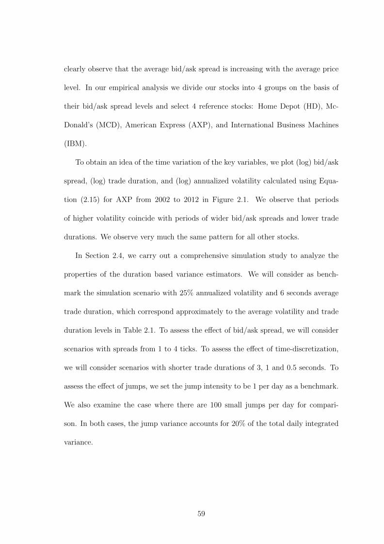
clearly observe that the average bid/ask spread is increasing with the average price
level. In our empirical analysis we divide our stocks into 4 groups on the basis of
their bid/ask spread levels and select 4 reference stocks: Home Depot (HD), Mc-
Donald’s (MCD), American Express (AXP), and International Business Machines
(IBM).
To obtain an idea of the time variation of the key variables, we plot (log) bid/ask
spread, (log) trade duration, and (log) annualized volatility calculated using Equa-
tion (2.15) for AXP from 2002 to 2012 in Figure 2.1. We observe that periods
of higher volatility coincide with periods of wider bid/ask spreads and lower trade
durations. We observe very much the same pattern for all other stocks.
In Section 2.4, we carry out a comprehensive simulation study to analyze the
properties of the duration based variance estimators. We will consider as bench-
mark the simulation scenario with 25% annualized volatility and 6 seconds average
trade duration, which correspond approximately to the average volatility and trade
duration levels in Table 2.1. To assess the effect of bid/ask spread, we will consider
scenarios with spreads from 1 to 4 ticks. To assess the effect of time-discretization,
we will consider scenarios with shorter trade durations of 3, 1 and 0.5 seconds. To
assess the effect of jumps, we set the jump intensity to be 1 per day as a benchmark.
We also examine the case where there are 100 small jumps per day for compari-
son. In both cases, the jump variance accounts for 20% of the total daily integrated
variance.
59
2.4 Simulation results
We separate the MMS noise into time-discretization (∆), bid/ask spread (ς), and
price-discretization components. We investigate the separate and combined effects
of the noise components as well as jumps on the non-parametric duration based
volatility estimator, NPDV (or NP for convenience), in a Monte Carlo study with
10,000 replications. Specifically, we assess the performance of the NP estimator
under different levels of: 1) time-discretization, 2) bid/ask spread, 3) jump size and
intensity.
The performance of the duration based integrated variance estimator depends on
the selection of a preferred threshold value. Following the discussion of the two main
sources of noise, bid/ask spread and time-discretization, we will discuss in Section
2.4.3 the tradeoff between efficiency and bias in the context of choosing a preferred
threshold value δ∗.
Finally, in Section 2.4.6 we compare through simulation the accuracy and effi-
ciency of the duration based variance estimator with other RV estimators, including
the Two-scaled RV (TSRV) and Realised Kernel (RK) estimators, which are also
included in Section 2.6 for volatility forecasting comparisons.
2.4.1 Time-discretization
Let us consider a discrete-time setting with a fixed time period, e.g. a trading day.
∆ is the discretization time interval and Yi∆ is the (noisy) price, i = 0, . . . ,M , where
M the number intraday periods. Yi∆ consists of a discretized efficient price process
Xi∆ and a noise component.
60
Discretizing Xt in (2.1), yields a time-discretized diffusion component
Xt −Xt−∆ = σX√
∆Zt. (2.20)
Zt is a standard normally distributed random variable and σX is the daily integrated
volatility, which is assumed to be constant.
In implementation, we first discretize the diffusion process on a half-second inter-
val so that there are 46800 efficient returns from a standard normal distribution in a
6.5-hour daily trading session. Upon this foundation process, we sample trade points
according to random Bernoulli distributions with probabilities 1/2, 1/6, and 1/12,
resulting in three other time-discretized processes with average inter-trade times ∆
of 1, 3, and 6 seconds respectively.
Ratios of the NP variance estimates over the true integrated variance are plotted
in Figure 2.2. We investigate how the average trade duration, ∆, and the thresh-
old value, δ, affect the time-discretization noise, keeping the annualized4 integrated
volatility at 25% and no price variation outside trading sessions.
Time-discretization decreases the number of events observed, due to the absence
of price points that may have defined price events. As ∆ decreases, the number of
price points increases and N approaches its true value (in the case when prices are
observed continuously). Thus, given δ, a smaller ∆ leads to more accurate estimates
of the integrated variance represented by the unit line in Figure 2.2, while increasing
δ for a given ∆ reduces the bias introduced by time-discretization.
4Using 252 trading days per year.
61
2.4.2 Bid/ask spread and time-discretization
As shown in Section 2.2.2, introduction of a bid/ask spread and corresponding bid
and ask transaction prices biases the duration based variance estimates upwards,
and the bias increases with the size of the spread ς, and decreases with the threshold
value δ when δ > ς. We now consider discrete time, with an average ∆ of 6 seconds,
bid and ask transaction prices generated by Yt = Pt+0.51tς, with σX corresponding
to 25% annualized volatility. The transaction price takes either the bid or the ask
side with probability 0.5 and the variables 1t are i.i.d.
Figure 2.3 shows ratios of the NP variance estimates over the true integrated
variance. A deviation from the unit line indicates a bias. The hump-shaped curves
occur as a result of the bid/ask spread component bias when the spread is relatively
large. When δ < ς, one bid/ask bounce is enough to trigger a price event and N is
inflated in comparison to the case when ς → 0 (dotted line). N does not decrease
much as δ increases as long as δ < ς, causing the NP estimate, Nδ2, to increase
rapidly, until δ = ς. When δ further increases so δ > ς, the influence of bid/ask
bounces is mitigated by the price changes from the efficient price component as
a price event is now increasingly caused by the cumulative efficient price changes
rather than by the bid/ask spread component. The bid/ask spread has the largest
influence around the point where δ = ς.
As δ increases past ς, the NP estimates start to stabilize, since both the time-
discretization and the bid/ask spread biases are reduced by larger threshold values
of δ. We observe two scenarios: 1) for smaller bid/ask spread levels (here 1 and
2 ticks) the negative bias contribution of the time-discretization is partially off-set
62
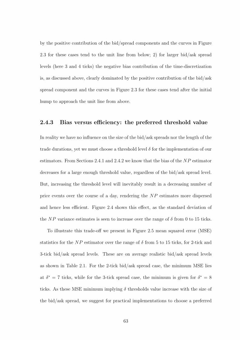
by the positive contribution of the bid/spread components and the curves in Figure
2.3 for these cases tend to the unit line from below; 2) for larger bid/ask spread
levels (here 3 and 4 ticks) the negative bias contribution of the time-discretization
is, as discussed above, clearly dominated by the positive contribution of the bid/ask
spread component and the curves in Figure 2.3 for these cases tend after the initial
hump to approach the unit line from above.
2.4.3 Bias versus efficiency: the preferred threshold value
In reality we have no influence on the size of the bid/ask spreads nor the length of the
trade durations, yet we must choose a threshold level δ for the implementation of our
estimators. From Sections 2.4.1 and 2.4.2 we know that the bias of the NP estimator
decreases for a large enough threshold value, regardless of the bid/ask spread level.
But, increasing the threshold level will inevitably result in a decreasing number of
price events over the course of a day, rendering the NP estimates more dispersed
and hence less efficient. Figure 2.4 shows this effect, as the standard deviation of
the NP variance estimates is seen to increase over the range of δ from 0 to 15 ticks.
To illustrate this trade-off we present in Figure 2.5 mean squared error (MSE)
statistics for the NP estimator over the range of δ from 5 to 15 ticks, for 2-tick and
3-tick bid/ask spread levels. These are on average realistic bid/ask spread levels
as shown in Table 2.1. For the 2-tick bid/ask spread case, the minimum MSE lies
at δ∗ = 7 ticks, while for the 3-tick spread case, the minimum is given for δ∗ = 8
ticks. As these MSE minimum implying δ thresholds value increase with the size of
the bid/ask spread, we suggest for practical implementations to choose a preferred
63
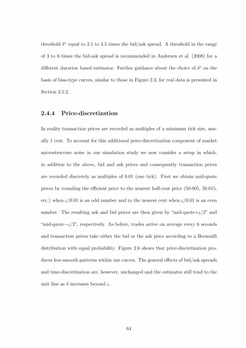
threshold δ∗ equal to 2.5 to 3.5 times the bid/ask spread. A threshold in the range
of 3 to 6 times the bid-ask spread is recommended in Andersen et al. (2008) for a
different duration based estimator. Further guidance about the choice of δ∗ on the
basis of bias-type curves, similar to those in Figure 2.3, for real data is presented in
Section 2.5.2.
2.4.4 Price-discretization
In reality transaction prices are recorded as multiples of a minimum tick size, usu-
ally 1 cent. To account for this additional price-discretization component of market
microstructure noise in our simulation study we now consider a setup in which,
in addition to the above, bid and ask prices and consequently transaction prices
are recorded discretely as multiples of 0.01 (one tick). First we obtain mid-quote
prices by rounding the efficient price to the nearest half-cent price (50.005, 50.015,
etc.) when ς/0.01 is an odd number and to the nearest cent when ς/0.01 is an even
number. The resulting ask and bid prices are then given by “mid-quote+ς/2” and
“mid-quote−ς/2”, respectively. As before, trades arrive on average every 6 seconds
and transaction prices take either the bid or the ask price according to a Bernoulli
distribution with equal probability. Figure 2.6 shows that price-discretization pro-
duces less smooth patterns within our curves. The general effects of bid/ask spreads
and time-discretization are, however, unchanged and the estimates still tend to the
unit line as δ increases beyond ς.
64
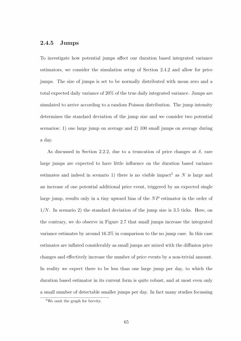
2.4.5 Jumps
To investigate how potential jumps affect our duration based integrated variance
estimators, we consider the simulation setup of Section 2.4.2 and allow for price
jumps. The size of jumps is set to be normally distributed with mean zero and a
total expected daily variance of 20% of the true daily integrated variance. Jumps are
simulated to arrive according to a random Poisson distribution. The jump intensity
determines the standard deviation of the jump size and we consider two potential
scenarios: 1) one large jump on average and 2) 100 small jumps on average during
a day.
As discussed in Section 2.2.2, due to a truncation of price changes at δ, rare
large jumps are expected to have little influence on the duration based variance
estimates and indeed in scenario 1) there is no visible impact5 as N is large and
an increase of one potential additional price event, triggered by an expected single
large jump, results only in a tiny upward bias of the NP estimator in the order of
1/N . In scenario 2) the standard deviation of the jump size is 3.5 ticks. Here, on
the contrary, we do observe in Figure 2.7 that small jumps increase the integrated
variance estimates by around 16.3% in comparison to the no jump case. In this case
estimates are inflated considerably as small jumps are mixed with the diffusion price
changes and effectively increase the number of price events by a non-trivial amount.
In reality we expect there to be less than one large jump per day, to which the
duration based estimator in its current form is quite robust, and at most even only
a small number of detectable smaller jumps per day. In fact many studies focussing
5We omit the graph for brevity.
65
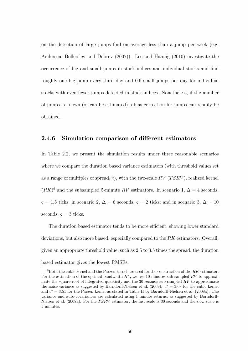
on the detection of large jumps find on average less than a jump per week (e.g.
Andersen, Bollerslev and Dobrev (2007)). Lee and Hannig (2010) investigate the
occurrence of big and small jumps in stock indices and individual stocks and find
roughly one big jump every third day and 0.6 small jumps per day for individual
stocks with even fewer jumps detected in stock indices. Nonetheless, if the number
of jumps is known (or can be estimated) a bias correction for jumps can readily be
obtained.
2.4.6 Simulation comparison of different estimators
In Table 2.2, we present the simulation results under three reasonable scenarios
where we compare the duration based variance estimators (with threshold values set
as a range of multiples of spread, ς), with the two-scale RV (TSRV ), realized kernel
(RK)6 and the subsampled 5-minute RV estimators. In scenario 1, ∆ = 4 seconds,
ς = 1.5 ticks; in scenario 2, ∆ = 6 seconds, ς = 2 ticks; and in scenario 3, ∆ = 10
seconds, ς = 3 ticks.
The duration based estimator tends to be more efficient, showing lower standard
deviations, but also more biased, especially compared to the RK estimators. Overall,
given an appropriate threshold value, such as 2.5 to 3.5 times the spread, the duration
based estimator gives the lowest RMSEs.
6Both the cubic kernel and the Parzen kernel are used for the construction of the RK estimator.For the estimation of the optimal bandwidth H∗, we use 10 minutes sub-sampled RV to approxi-mate the square-root of integrated quarticity and the 30 seconds sub-sampled RV to approximatethe noise variance as suggested by Barndorff-Nielsen et al. (2009). c∗ = 3.68 for the cubic kerneland c∗ = 3.51 for the Parzen kernel as stated in Table II by Barndorff-Nielsen et al. (2008a). Thevariance and auto-covariances are calculated using 1 minute returns, as suggested by Barndorff-Nielsen et al. (2008a). For the TSRV estimator, the fast scale is 30 seconds and the slow scale is5 minutes.
66
2.5 Empirical analysis
2.5.1 Parametric duration based variance estimator
For the implementation of the parametric duration based variance estimator, PDV ,
we consider three distributional assumptions for εd in equation (2.9): Exponential,
Weibull, and Burr distributions. Price durations are obtained for a range of threshold
values δ and are scaled each month, as described after equation (2.14), using a daily
seasonality function obtained from a Nadaraya-Watson kernel regression. Maximum
likelihood estimations (MLE) of the duration models represented by equations (2.9)
and (2.10) under the three distributional assumptions are performed on a monthly
basis.
We perform likelihood ratio (LR), Ljung-Box (LB), and density forecast (DF)
tests to assess the goodness-of-fit of the models. The LR test compares the overall
model fit between two nested models on the basis of their likelihood values. The LB
test has the null hypothesis of i.i.d. distributed εd. The DF test of Diebold et al.
(1998) tests the null hypothesis that the assumed distribution for εd is actually the
true distribution and relies on a probability integral transformation of εd, namely
the c.d.f. F (εd), which under the null is i.i.d. U(0, 1) distributed. Provided that
the HACD specification in (2.10) accommodates long-range dependence of the price
durations data appropriately, and the assumed distribution for εd reflects the true
distribution of the scaled duration, neither the LB nor the DF test should be rejected.
All tests are performed, for each of the 132 months from January 2002 to Decem-
ber 2012, over a selected range of δ threshold values (between 2 to up to 20 ticks) for
67
four reference stocks: HD, MCD, AXP and IBM. In the interest of brevity, all tests
results are relegated to the Appendix. The conclusion is unequivocal: conditional
Burr distributions fit the price durations data best. As an illustration, Table 2.3
presents the parameter values for the Burr-HACD model for AXP in 2008, with δ
equal to 12 ticks, together with LB and DF tests results. As expected, we observe
that, although there is some variation over the months, generally price durations are
very persistent with an average β1 equal to 0.64 and an average α equal to 0.22. The
parameters η and γ have values that are significantly different from 0 and 1, respec-
tively, which shows that the Burr specification provides a better fit than the Weibull
or Exponential specifications. The LB tests’ p-values at lag 50 for the generalized
model residuals indicate that the null hypotheses can only be rejected in 2 out of
12 cases at a 5% significance level and shows that generally the HACD specification
dynamics provides a satisfactory fit. The density forecasting tests’ p-values reveal
that the null hypotheses can be rejected in 5 out of 12 cases at the 5% level and indi-
cates that there is scope to further improve, especially through the choice of a more
flexible density function for εd, upon the Burr-HACD specification. The selection of
more flexible densities than the Burr density usually comes with the cost of losing
some computational tractability and we refrain from considering them in this paper.
Taken together, the fit provided by the Burr-HACD specification is good, also in the
light of Section 2.6 that focuses on out-of-sample forecasting comparisons.
68
2.5.2 The preferred threshold value
As discussed in Section 2.4.3, the selection of δ∗ needs to take into account the
tradeoff between improving efficiency and reducing bias: a larger δ reduces bias
while a smaller δ improves efficiency. In the simulation study we know the true
value of the integrated variance, and their MSE statistics for sensible simulation
setups suggest that a threshold value δ∗ should preferably be chosen to lie within
the range of 2.5 to 3.5 times the bid/ask spread. In this section we provide a number
of selective empirical results that support the conclusions of the simulation study
and provide further guidance on how to select a preferred threshold δ∗. The results
presented in this section focus on the reference stock AXP.7
We start by considering NP variance estimates in October 2008, when volatility
peaked during the financial crisis. This month is governed by high uncertainty and
average bid/ask spread levels of 4.6 ticks in this month are amongst the highest
in our sample period. Figure 2.8 plots the NP variance estimates for the first 20
trading days of October 2008 for stock AXP, over the range of threshold values from
2 ticks to 15 ticks. We observe that, even during this high bid/ask spread level
regime, duration based variance estimates first increase with the chosen threshold
value and then stabilize, which is a stabilizing pattern that is similar to the one
shown in Figure 2.3 for the simulation setting.
The results of the simulation study suggest that estimates are less biased once
stabilization has been achieved and pinpointing the lower bound of this stabilizing
region would provide a good trade-off between bias and efficiency and a good choice
7Results for the other stocks are available from the authors upon request.
69
for the preferred threshold value δ∗. To obtain a better picture of this stabilizing
behavior, and its relationship to the level of the bid/ask spread in reality, we consider
the full data sample for AXP. We divide the 132 months into 6 groups based on
their average spread levels and obtain for each group daily NP variance estimates
(annualized) for δ between 2 and 15 ticks and show their averages across days in
Figure 2.9. The 6 groups represent in ascending average spread level order the lower
1/3, the middle 1/3 and then the upper 1/3, subdivided into 4 ascending groups
(1/12 each), of the data. Table 2.4 shows the distribution of the 6 groups across the
132 month in the data sample. It should be noted that many of the high bid/ask
spread level months, besides the ones during the financial crisis, are in the early
years of the data sample when trading was less liquid, and consequently many of the
low bid/ask spread level months are concentrated at the end of the data sample.
Figure 2.9 shows the stabilizing behavior of the duration based variance estimates
very clearly and, upon visual inspection, we observe that the threshold value at the
point where the estimates start to stabilize, δ∗, is roughly three times the average
bid/ask spread which is in line with the guidance obtained from the simulation study.
We will use the “three-times-bid/ask-spread” rule henceforth as guidance to select δ∗
for the computation of the PDV and NP estimators in the subsequent forecasting
study.
Table 2.19 in the Appendix presents goodness-of-fit results (LB and DF tests) of
the Burr-HACD model for all 20 stocks, with the price durations obtained by setting
the threshold value to be δ∗. It confirms that, when the threshold value is set to
be three times the average bid/ask-spread, the Burr-HACD fits the price durations
70
data well.
2.6 Volatility forecasts evaluation
To assess the quality of our duration based variance estimators we conduct a compre-
hensive forecasting study. We compare our duration based variance estimators with
variance estimators from two other important classes: RV -type and option-implied.
Our target volatility measures are the realized one-day, one-week, and one-month
ahead 5-minute realized volatilities. From the class of duration based variance es-
timators we consider the PDV estimator based on the Burr-HACD specification
discussed above, with parameters estimated monthly, variance estimates computed
on the basis of previous month parameter values and δ∗ equal to three times the
bid/ask spread of the previous month to avoid any forward information bias. We
also consider NP variance estimators with δ∗ equal to three times the bid/ask spread
of the previous day, NPd, and δ∗ equal to three times the bid/ask spread of the pre-
vious month, NPm. From the class of RV -type variance estimators we consider a
realised kernel, RK, a two-scale realized variance, TSRV , a bi-power realized vari-
ance, BV , and a sub-sampled 5 minute realized variance, RV , estimator.8 From
the class of option-implied variance estimators we consider an at-the-money implied
volatility, ATM , a model free implied volatility (with implied volatility curves fitted
as a quadratic function of delta), MFIV2, and a second model free implied volatil-
ity estimator obtained from cubic functions of delta, MFIV3.9 In the interest of
8The cubic kernel is used here. The construction of the RK and TSRV estimators is the sameas described in Section 2.4.6.
9The options data, which cover the same time period as the high-frequency trades and quotesdata, are obtained from the OptionMetrics database. We directly employ the Black-Scholes implied
71
brevity, we present results only for the best performing estimators in the RV -type
and option-implied classes10: RK and ATM . We find that the ATM option-implied
volatility estimator gives more accurate forecasts of future volatility than both model
free option-implied volatility estimators. This result is consistent with the finding
of Martin et al. (2009) showing that when three individual stocks are considered
ATM estimators outperform model free estimators. For stock indices, as for exam-
ple considered by Jiang and Tian (2005), model free estimators are usually found
to show superior forecasting performance. In contrast to individual stocks, there is
normally a more liquid and larger set of index options available, which allows for a
more accurate approximation of the delta-implied-volatility-curves necessary for the
construction of model free estimators. In the analysis below all estimators are used
in an annualized form.
2.6.1 Individual forecasts
We employ a HAR-type forecasting equation,
RVn:n+h = c+ b1Zn−1 + b2Zn−5:n−1 + b3Zn−22:n−1 + εn:n+h. (2.21)
volatility (IV ), including the at-the-money implied volatility, provided by OptionMetrics. Weretain options with time-to-maturities between 7 and 42 calendar days, and with positive bid-quotes and positive bid-ask spreads. Nearest-to-maturity options are usually chosen, but if theyprovide less than four (five) IV ’s for fitting the quadratic (cubic) curve, we switch to the secondnearest-to-maturity day. For the construction of the model-free implied volatility estimator, wefollow Taylor et al. (2010) and estimate the IV curve as a function of the Black-Scholes delta. Weconstruct two versions of MFIV by fitting quadratic and cubic functions to the delta-IV curves.To prevent delta/IV points from clustering on one side of the curve, we require at least four (five)delta/IV observations a day, and at least one delta below 0.3, at least one above 0.7, and at leastone between 0.3 and 0.7. In addition, we exclude extreme deltas larger than 0.99 or smaller than0.01.
10Results for the other estimators can be obtained from the authors upon request.
72
Here Zn represents the day-n volatility estimate from one of the five estimators dis-
cussed above (PDV , NPd, NPm, RK, ATM). Both Zn−h:n−1 and RVn:n+h aggregate
h terms and are in their logarithmic forms: Zn−h:n−1 = 0.5 log(∑n−1s=n−h Z
2s ), similarly
for RVn:n+h, h=1,5, or 22, with RVn the day-n 5-minute realized volatility. For one
day (h = 1) ahead forecasts the in-sample estimation period for the HAR model
ranges from 1 February 2002 to 29 January 2010 (2013 trading days) and the first
out-of-sample forecast is obtained for 1 February 2010. For one week (h = 5) and
one month (h = 22) horizons forecasts are constructed similarly and a total of 735,
731 and 714 out-of-sample predictions are obtained for h = 1, 5 and 22, respectively,
with the final predictions made in December 2012. All forecasts are constructed
using a rolling window of explanatory variables.
Figures 2.10, 2.11, and 2.12 show root-mean-squared-errors, RMSE, of the fore-
casts from the five different estimators, for one day, one week, and one month hori-
zons. The 20 firms on the horizontal axis are sorted in ascending order of their
RMSEs obtained from the PDV estimator.
Over all three forecasting horizons, PDV generally produces the lowest RMSEs.
To assess whether two competing forecasts perform significantly differently we per-
form a modified Diebold-Mariano (DM) test, using a squared error loss function.
The DM test tests the null hypothesis of equal predictive ability of two competing
forecasts by assessing the significance of their average loss differentials. For the 5%
significance level, results are presented in Table 2.5. Each figure counts the num-
ber of significantly negative/positive loss differentials out of the 20 firms for the
corresponding (estimators) pair in the first row. The figures in the “−”, “+” rows
73
respectively count the number of firms that favor the first and second estimator.
The first three columns compare forecasts based on the three estimators from
the duration based variance class. Over all three horizons PDV estimators lead
to significantly more accurate forecasts than the two corresponding nonparametric
duration based variance estimators. Note that a NP estimator for a given day uses
only information from this specific day, while the PDV estimator for a given day
uses additionally also information from past price durations for example through
the dynamic Burr-HACD specification. Hence, the PDV estimator is based on a
richer information set whose exploitation yields more precise variance estimators
and consequently more accurate forecasts. The information advantage of this richer
information set (together with a careful Burr-HACD model selection) also seems to
dominate any additional model estimation noise from estimating the Burr-HACD
specification. Moreover, NPm performs better than NPd which could stem from
a smoothing effect of NPm as it uses monthly average bid/ask spread levels to
construct δ∗ while NPd relies on daily average bid/ask spread levels that are more
volatile.
Columns 4-6 compare forecasts of duration based variance estimators with those
from RK. PDV leads to more precise forecasts than RK over all three horizons. The
two non-parametric estimators perform better than RK over the one-day horizon,
on par with RK over the one-week horizon, and are marginally better over the
one-month horizon.
Columns 7-9 compare forecasts of duration based variance estimators with those
from ATM option-implied variance estimators. Also here, the duration based vari-
74

ance estimators generally produce more accurate forecasts than ATM over all three
horizons.
The last column compares forecasts from ATM with those from RK. RK shows
better performance than ATM over the one-day and one-week horizons but performs
on par with ATM over the one-month horizon. ATM estimators perform better as
the forecasting horizon extends to one month. Forecasting comparisons between the
ATM option-implied volatility estimators and the RV estimators constructed from
historical high-frequency returns are well documented in the existing literature. For
example, Blair et al. (2001), Pong et al. (2004), and Taylor et al. (2010) find that,
when the forecast horizon matches the maturity of the corresponding options, which
is usually chosen to be around one month, the option-implied volatility estimator
shows a better forecasting performance than estimators constructed from historical
return data. Martin et al. (2009) and Busch et al. (2011) compare noise- and jump-
robust RV measures, including RK, TSRV and BV , with ATM and draw similar
conclusions. Over the one-month horizon, we find that RK and ATM perform
similarly and hence we do not find ATM to be a superior predictor of the one-
month ahead future volatility.
Overall, among individual volatility estimators, PDV gives the most accurate
forecasts over all three horizons. The easy-to-construct non-parametric duration
based variance estimators also outperform the established RK and ATM variance
estimators in most cases. We conclude that the duration-variance estimators can
extract information for integrated variance estimation and forecasting better than
RV -type and option-implied variance estimators.
75
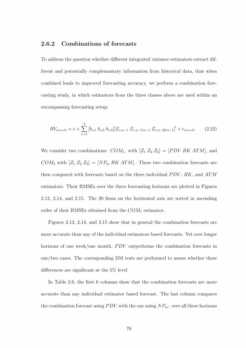
2.6.2 Combinations of forecasts
To address the question whether different integrated variance estimators extract dif-
ferent and potentially complementary information from historical data, that when
combined leads to improved forecasting accuracy, we perform a combination fore-
casting study, in which estimators from the three classes above are used within an
encompassing forecasting setup:
RVn:n+h = c+3∑v=1
[bv,1 bv,2 bv,3][Zv,n−1 Zv,n−5:n−1 Zv,n−22:n−1]′ + εn:n+h. (2.22)
We consider two combinations: COM1, with [Z1 Z2 Z3] = [PDV RK ATM ], and
COM2 with [Z1 Z2 Z3] = [NPm RK ATM ]. These two combination forecasts are
then compared with forecasts based on the three individual PDV , RK, and ATM
estimators. Their RMSEs over the three forecasting horizons are plotted in Figures
2.13, 2.14, and 2.15. The 20 firms on the horizontal axis are sorted in ascending
order of their RMSEs obtained from the COM1 estimator.
Figures 2.13, 2.14, and 2.15 show that in general the combination forecasts are
more accurate than any of the individual estimators based forecasts. Yet over longer
horizons of one week/one month, PDV outperforms the combination forecasts in
one/two cases. The corresponding DM tests are performed to assess whether these
differences are significant at the 5% level.
In Table 2.6, the first 6 columns show that the combination forecasts are more
accurate than any individual estimator based forecast. The last column compares
the combination forecast using PDV with the one using NPm: over all three horizons
76
and as established from the comparison above of the single estimator forecasts, the
PDV -based combination forecast is more accurate.
Taken together, combining information from different sources improves forecast
accuracy, and the parametric duration based variance estimator seems to extract
relevant information better than the nonparametric estimator.
2.7 Conclusion
Duration based variance estimators are calculated by using the times of price change
events; an event occurs when the magnitude of the price change since the previous
event first equals or exceeds some threshold value. These estimators have been ne-
glected in previous research, despite their potentially superior efficiency compared
with realized variance estimators. The potential for superior efficiency occurs be-
cause duration based estimators make use of the complete path of prices, while
standard RV estimators discard almost all prices for liquid securities such as the
DJIA stocks studied in this paper. Market microstructure noise obscures theoreti-
cal comparisons and, furthermore, requires careful consideration to be given to the
selection of the threshold value.
We use both Monte Carlo methods and real price data to recommend that an
appropriate choice of the threshold is three times a measure of the average bid/ask
spread. For this choice, duration based estimators have relatively small bias and
relatively high efficiency (i.e. low mean squared error). We propose both parametric
and nonparametric duration based estimators and find that they both forecast fu-
ture volatility more accurately than either RV -type estimators or implied-volatility
77
estimators for three forecast horizons (one day, one week and one month), when the
forecasts are out-of-sample predictions from heterogeneous autoregressive models.
Diebold-Mariano tests show that many of the forecast improvements are significant
at the 5% level; for example, comparing the parametric duration estimator with the
realized kernel estimator gives 10 significant results for the 20 stocks studied at a
one-day horizon, 10 significant for the one-week horizon and 5 significant for the
one-month horizon, with all significant differences favouring the duration estimator.
Calculation of the nonparametric duration estimator from a complete record of
transaction prices is a trivial task. The parametric estimator is more accurate but
does require the estimation of a parametric model for price events, which requires
specifying intensity functions for durations whose conditional expectations are func-
tions of previous durations. We recommend considering duration based estimators
of integrated variation whenever transaction prices are available because of their
potential to provide more accurate estimates and forecasts.
The duration based variance estimates are generally more biased than competing
estimators. Further research shall be undertaken to reduce the bias of the variance
estimates using price durations. The bias of the duration based variance estima-
tors stems partly from the insufficiency of transaction price data, due to the time-
discretization noise. Thus experiments can be undertaken on quote data, which may
contain less time-discretization as well as bid/ask spread noise.
78
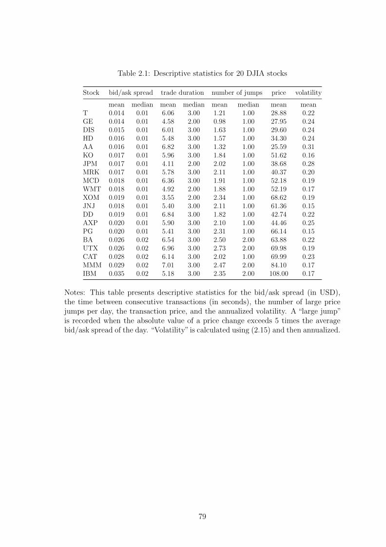
Table 2.1: Descriptive statistics for 20 DJIA stocks
Stock bid/ask spread trade duration number of jumps price volatility
mean median mean median mean median mean meanT 0.014 0.01 6.06 3.00 1.21 1.00 28.88 0.22GE 0.014 0.01 4.58 2.00 0.98 1.00 27.95 0.24DIS 0.015 0.01 6.01 3.00 1.63 1.00 29.60 0.24HD 0.016 0.01 5.48 3.00 1.57 1.00 34.30 0.24AA 0.016 0.01 6.82 3.00 1.32 1.00 25.59 0.31KO 0.017 0.01 5.96 3.00 1.84 1.00 51.62 0.16JPM 0.017 0.01 4.11 2.00 2.02 1.00 38.68 0.28MRK 0.017 0.01 5.78 3.00 2.11 1.00 40.37 0.20MCD 0.018 0.01 6.36 3.00 1.91 1.00 52.18 0.19WMT 0.018 0.01 4.92 2.00 1.88 1.00 52.19 0.17XOM 0.019 0.01 3.55 2.00 2.34 1.00 68.62 0.19JNJ 0.018 0.01 5.40 3.00 2.11 1.00 61.36 0.15DD 0.019 0.01 6.84 3.00 1.82 1.00 42.74 0.22AXP 0.020 0.01 5.90 3.00 2.10 1.00 44.46 0.25PG 0.020 0.01 5.41 3.00 2.31 1.00 66.14 0.15BA 0.026 0.02 6.54 3.00 2.50 2.00 63.88 0.22UTX 0.026 0.02 6.96 3.00 2.73 2.00 69.98 0.19CAT 0.028 0.02 6.14 3.00 2.02 1.00 69.99 0.23MMM 0.029 0.02 7.01 3.00 2.47 2.00 84.10 0.17IBM 0.035 0.02 5.18 3.00 2.35 2.00 108.00 0.17
Notes: This table presents descriptive statistics for the bid/ask spread (in USD),the time between consecutive transactions (in seconds), the number of large pricejumps per day, the transaction price, and the annualized volatility. A “large jump”is recorded when the absolute value of a price change exceeds 5 times the averagebid/ask spread of the day. “Volatility” is calculated using (2.15) and then annualized.
79
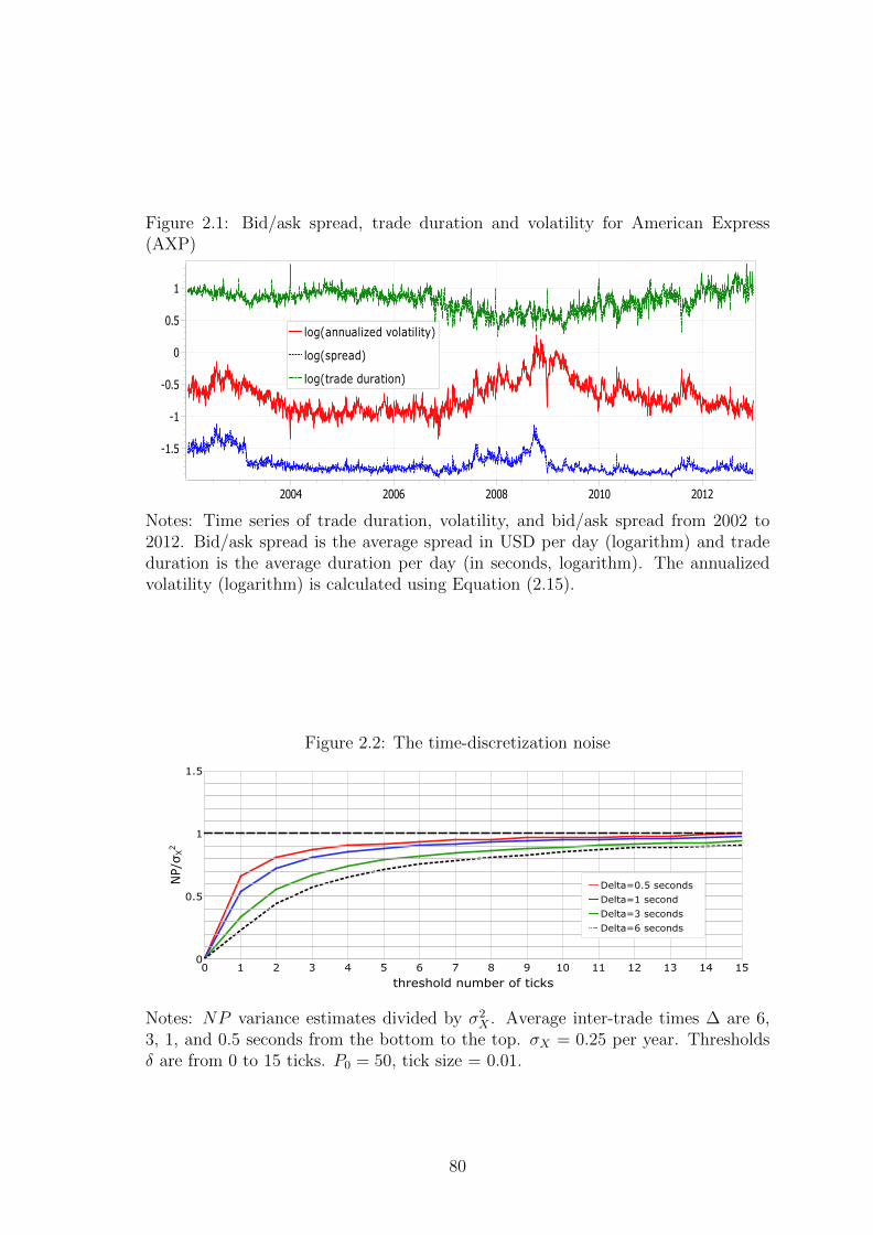
Figure 2.1: Bid/ask spread, trade duration and volatility for American Express(AXP)
-1.5
-1
-0.5
0
0.5
1
2004 2006 2008 2010 2012
log(annualized volatility)
log(spread)
log(trade duration)
Notes: Time series of trade duration, volatility, and bid/ask spread from 2002 to2012. Bid/ask spread is the average spread in USD per day (logarithm) and tradeduration is the average duration per day (in seconds, logarithm). The annualizedvolatility (logarithm) is calculated using Equation (2.15).
Figure 2.2: The time-discretization noise
Notes: NP variance estimates divided by σ2X . Average inter-trade times ∆ are 6,
3, 1, and 0.5 seconds from the bottom to the top. σX = 0.25 per year. Thresholdsδ are from 0 to 15 ticks. P0 = 50, tick size = 0.01.
80
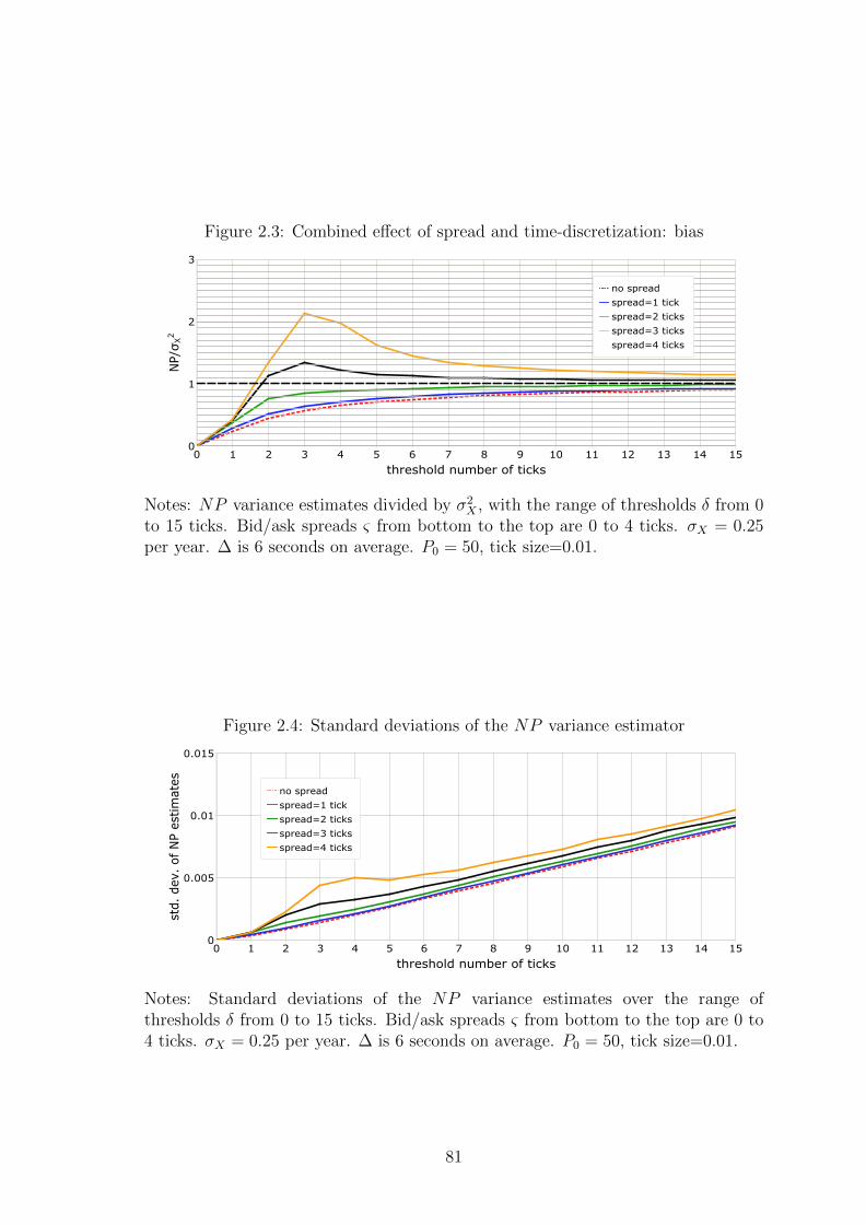
Figure 2.3: Combined effect of spread and time-discretization: bias
Notes: NP variance estimates divided by σ2X , with the range of thresholds δ from 0
to 15 ticks. Bid/ask spreads ς from bottom to the top are 0 to 4 ticks. σX = 0.25per year. ∆ is 6 seconds on average. P0 = 50, tick size=0.01.
Figure 2.4: Standard deviations of the NP variance estimator
Notes: Standard deviations of the NP variance estimates over the range ofthresholds δ from 0 to 15 ticks. Bid/ask spreads ς from bottom to the top are 0 to4 ticks. σX = 0.25 per year. ∆ is 6 seconds on average. P0 = 50, tick size=0.01.
81
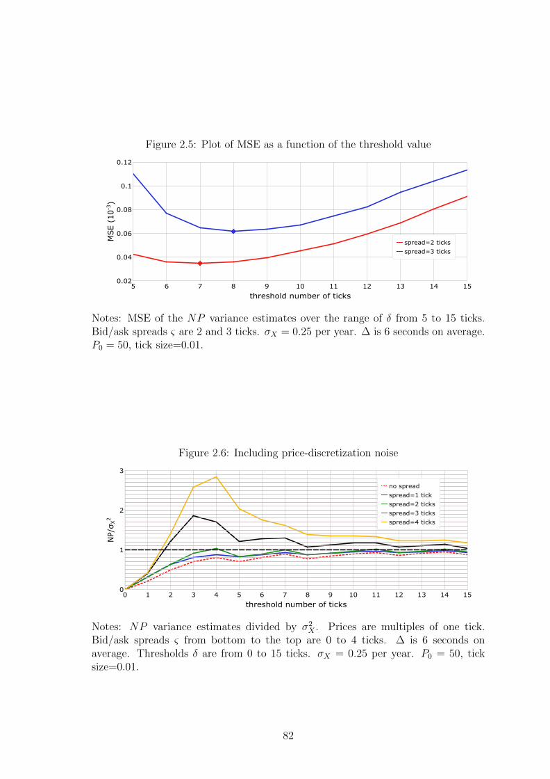
Figure 2.5: Plot of MSE as a function of the threshold value
Notes: MSE of the NP variance estimates over the range of δ from 5 to 15 ticks.Bid/ask spreads ς are 2 and 3 ticks. σX = 0.25 per year. ∆ is 6 seconds on average.P0 = 50, tick size=0.01.
Figure 2.6: Including price-discretization noise
Notes: NP variance estimates divided by σ2X . Prices are multiples of one tick.
Bid/ask spreads ς from bottom to the top are 0 to 4 ticks. ∆ is 6 seconds onaverage. Thresholds δ are from 0 to 15 ticks. σX = 0.25 per year. P0 = 50, ticksize=0.01.
82
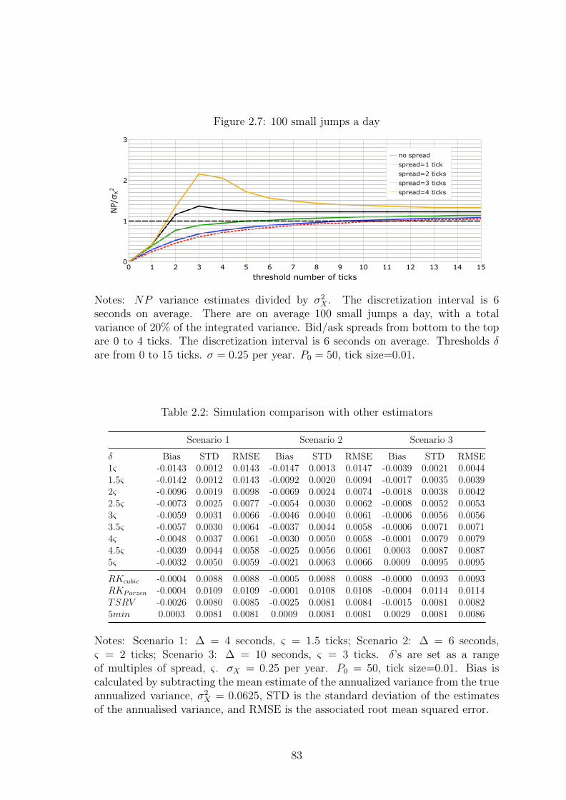
Figure 2.7: 100 small jumps a day
Notes: NP variance estimates divided by σ2X . The discretization interval is 6
seconds on average. There are on average 100 small jumps a day, with a totalvariance of 20% of the integrated variance. Bid/ask spreads from bottom to the topare 0 to 4 ticks. The discretization interval is 6 seconds on average. Thresholds δare from 0 to 15 ticks. σ = 0.25 per year. P0 = 50, tick size=0.01.
Table 2.2: Simulation comparison with other estimators
Scenario 1 Scenario 2 Scenario 3
δ Bias STD RMSE Bias STD RMSE Bias STD RMSE1ς -0.0143 0.0012 0.0143 -0.0147 0.0013 0.0147 -0.0039 0.0021 0.00441.5ς -0.0142 0.0012 0.0143 -0.0092 0.0020 0.0094 -0.0017 0.0035 0.00392ς -0.0096 0.0019 0.0098 -0.0069 0.0024 0.0074 -0.0018 0.0038 0.00422.5ς -0.0073 0.0025 0.0077 -0.0054 0.0030 0.0062 -0.0008 0.0052 0.00533ς -0.0059 0.0031 0.0066 -0.0046 0.0040 0.0061 -0.0006 0.0056 0.00563.5ς -0.0057 0.0030 0.0064 -0.0037 0.0044 0.0058 -0.0006 0.0071 0.00714ς -0.0048 0.0037 0.0061 -0.0030 0.0050 0.0058 -0.0001 0.0079 0.00794.5ς -0.0039 0.0044 0.0058 -0.0025 0.0056 0.0061 0.0003 0.0087 0.00875ς -0.0032 0.0050 0.0059 -0.0021 0.0063 0.0066 0.0009 0.0095 0.0095
RKcubic -0.0004 0.0088 0.0088 -0.0005 0.0088 0.0088 -0.0000 0.0093 0.0093RKParzen -0.0004 0.0109 0.0109 -0.0001 0.0108 0.0108 -0.0004 0.0114 0.0114TSRV -0.0026 0.0080 0.0085 -0.0025 0.0081 0.0084 -0.0015 0.0081 0.00825min 0.0003 0.0081 0.0081 0.0009 0.0081 0.0081 0.0029 0.0081 0.0086
Notes: Scenario 1: ∆ = 4 seconds, ς = 1.5 ticks; Scenario 2: ∆ = 6 seconds,ς = 2 ticks; Scenario 3: ∆ = 10 seconds, ς = 3 ticks. δ’s are set as a rangeof multiples of spread, ς. σX = 0.25 per year. P0 = 50, tick size=0.01. Bias iscalculated by subtracting the mean estimate of the annualized variance from the trueannualized variance, σ2
X = 0.0625, STD is the standard deviation of the estimatesof the annualised variance, and RMSE is the associated root mean squared error.
83
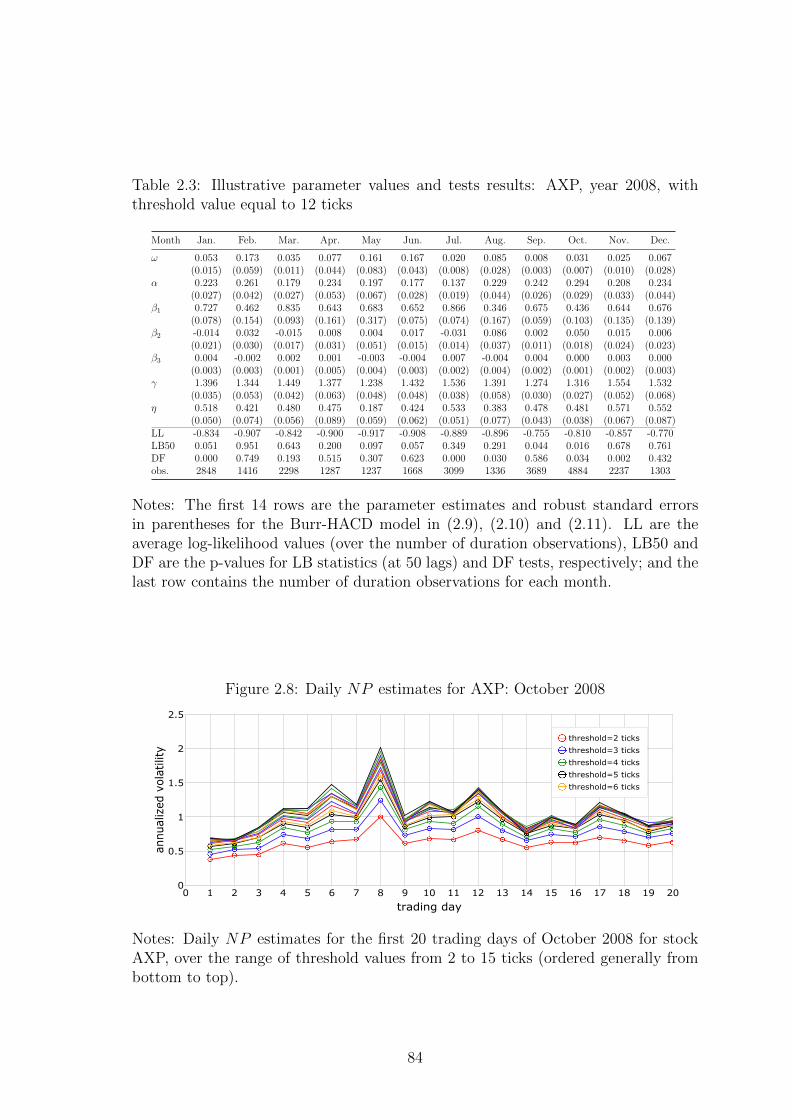
Table 2.3: Illustrative parameter values and tests results: AXP, year 2008, withthreshold value equal to 12 ticks
Month Jan. Feb. Mar. Apr. May Jun. Jul. Aug. Sep. Oct. Nov. Dec.
ω 0.053 0.173 0.035 0.077 0.161 0.167 0.020 0.085 0.008 0.031 0.025 0.067(0.015) (0.059) (0.011) (0.044) (0.083) (0.043) (0.008) (0.028) (0.003) (0.007) (0.010) (0.028)
α 0.223 0.261 0.179 0.234 0.197 0.177 0.137 0.229 0.242 0.294 0.208 0.234(0.027) (0.042) (0.027) (0.053) (0.067) (0.028) (0.019) (0.044) (0.026) (0.029) (0.033) (0.044)
β1 0.727 0.462 0.835 0.643 0.683 0.652 0.866 0.346 0.675 0.436 0.644 0.676(0.078) (0.154) (0.093) (0.161) (0.317) (0.075) (0.074) (0.167) (0.059) (0.103) (0.135) (0.139)
β2 -0.014 0.032 -0.015 0.008 0.004 0.017 -0.031 0.086 0.002 0.050 0.015 0.006(0.021) (0.030) (0.017) (0.031) (0.051) (0.015) (0.014) (0.037) (0.011) (0.018) (0.024) (0.023)
β3 0.004 -0.002 0.002 0.001 -0.003 -0.004 0.007 -0.004 0.004 0.000 0.003 0.000(0.003) (0.003) (0.001) (0.005) (0.004) (0.003) (0.002) (0.004) (0.002) (0.001) (0.002) (0.003)
γ 1.396 1.344 1.449 1.377 1.238 1.432 1.536 1.391 1.274 1.316 1.554 1.532(0.035) (0.053) (0.042) (0.063) (0.048) (0.048) (0.038) (0.058) (0.030) (0.027) (0.052) (0.068)
η 0.518 0.421 0.480 0.475 0.187 0.424 0.533 0.383 0.478 0.481 0.571 0.552(0.050) (0.074) (0.056) (0.089) (0.059) (0.062) (0.051) (0.077) (0.043) (0.038) (0.067) (0.087)
LL -0.834 -0.907 -0.842 -0.900 -0.917 -0.908 -0.889 -0.896 -0.755 -0.810 -0.857 -0.770LB50 0.051 0.951 0.643 0.200 0.097 0.057 0.349 0.291 0.044 0.016 0.678 0.761DF 0.000 0.749 0.193 0.515 0.307 0.623 0.000 0.030 0.586 0.034 0.002 0.432obs. 2848 1416 2298 1287 1237 1668 3099 1336 3689 4884 2237 1303
Notes: The first 14 rows are the parameter estimates and robust standard errorsin parentheses for the Burr-HACD model in (2.9), (2.10) and (2.11). LL are theaverage log-likelihood values (over the number of duration observations), LB50 andDF are the p-values for LB statistics (at 50 lags) and DF tests, respectively; and thelast row contains the number of duration observations for each month.
Figure 2.8: Daily NP estimates for AXP: October 2008
Notes: Daily NP estimates for the first 20 trading days of October 2008 for stockAXP, over the range of threshold values from 2 to 15 ticks (ordered generally frombottom to top).
84
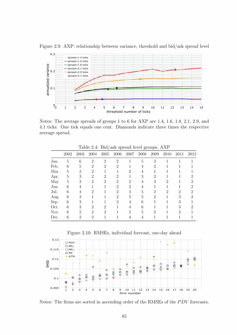
Figure 2.9: AXP: relationship between variance, threshold and bid/ask spread level
Notes: The average spreads of groups 1 to 6 for AXP are 1.4, 1.6, 1.8, 2.1, 2.9, and4.1 ticks. One tick equals one cent. Diamonds indicate three times the respectiveaverage spread.
Table 2.4: Bid/ask spread level groups, AXP
2002 2003 2004 2005 2006 2007 2008 2009 2010 2011 2012
Jan. 5 6 2 2 2 1 5 3 1 1 1Feb. 6 5 2 2 2 1 4 2 1 1 1Mar. 5 2 2 1 1 2 4 1 1 1 1Apr. 5 3 2 2 2 1 3 2 1 1 2May 5 3 2 2 2 2 4 3 2 1 2Jun. 6 4 1 1 2 2 4 1 1 1 2Jul. 6 4 2 1 2 4 5 2 2 2 2Aug. 6 3 1 1 2 5 5 2 1 3 2Sep. 6 3 1 1 2 4 6 1 1 3 1Oct. 6 3 2 2 1 4 6 1 1 3 2Nov. 6 2 2 2 1 5 5 2 1 2 1Dec. 6 2 2 1 1 4 4 1 1 1 1
Figure 2.10: RMSEs, individual forecast, one-day ahead
Notes: The firms are sorted in ascending order of the RMSEs of the PDV forecasts.
85
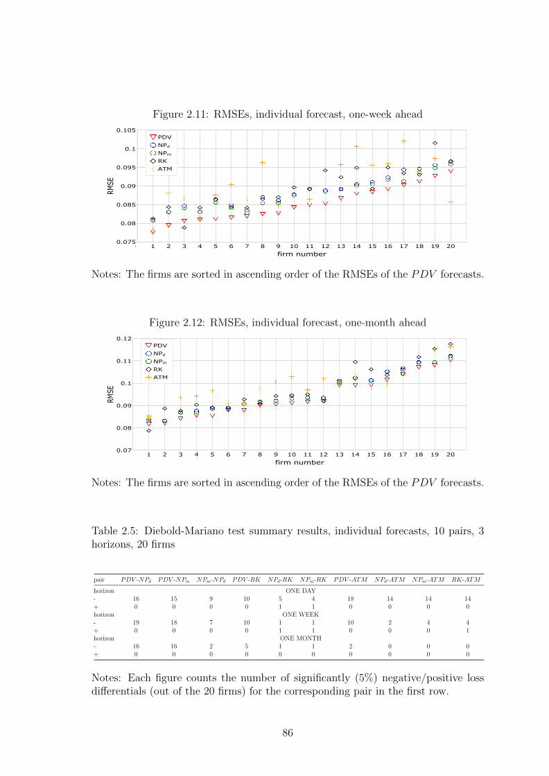
Figure 2.11: RMSEs, individual forecast, one-week ahead
Notes: The firms are sorted in ascending order of the RMSEs of the PDV forecasts.
Figure 2.12: RMSEs, individual forecast, one-month ahead
Notes: The firms are sorted in ascending order of the RMSEs of the PDV forecasts.
Table 2.5: Diebold-Mariano test summary results, individual forecasts, 10 pairs, 3horizons, 20 firms
pair PDV -NPd PDV -NPm NPm-NPd PDV -RK NPd-RK NPm-RK PDV -ATM NPd-ATM NPm-ATM RK-ATM
horizon ONE DAY- 16 15 9 10 5 4 18 14 14 14+ 0 0 0 0 1 1 0 0 0 0horizon ONE WEEK- 19 18 7 10 1 1 10 2 4 4+ 0 0 0 0 1 1 0 0 0 1horizon ONE MONTH- 16 16 2 5 1 1 2 0 0 0+ 0 0 0 0 0 0 0 0 0 0
Notes: Each figure counts the number of significantly (5%) negative/positive lossdifferentials (out of the 20 firms) for the corresponding pair in the first row.
86
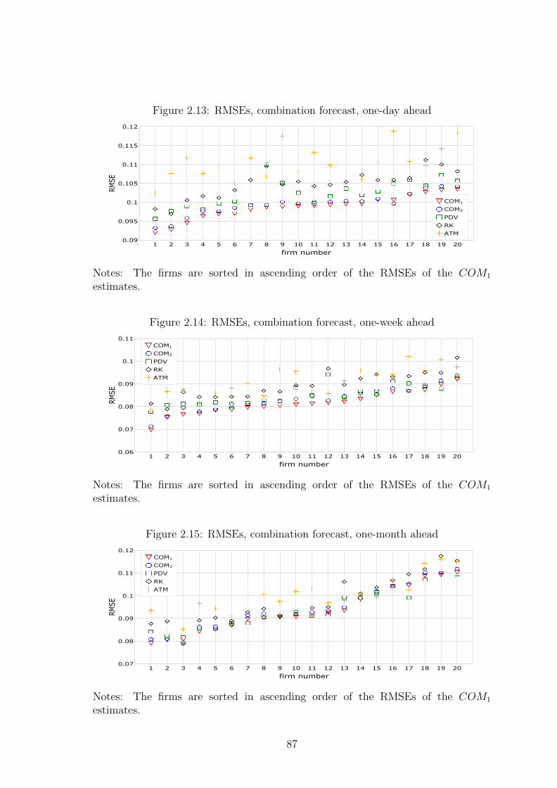
Figure 2.13: RMSEs, combination forecast, one-day ahead
Notes: The firms are sorted in ascending order of the RMSEs of the COM1estimates.
Figure 2.14: RMSEs, combination forecast, one-week ahead
Notes: The firms are sorted in ascending order of the RMSEs of the COM1estimates.
Figure 2.15: RMSEs, combination forecast, one-month ahead
Notes: The firms are sorted in ascending order of the RMSEs of the COM1estimates.
87
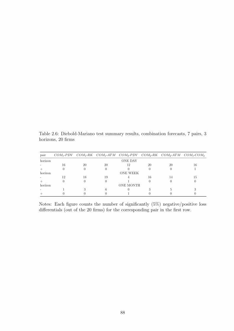
Table 2.6: Diebold-Mariano test summary results, combination forecasts, 7 pairs, 3horizons, 20 firms
pair COM1-PDV COM1-RK COM1-ATM COM2-PDV COM2-RK COM2-ATM COM1-COM2
horizon ONE DAY- 16 20 20 12 20 20 16+ 0 0 0 0 0 0 1horizon ONE WEEK- 12 18 19 4 16 14 15+ 0 0 0 1 0 0 0horizon ONE MONTH- 1 3 6 0 3 5 3+ 0 0 0 1 0 0 0
Notes: Each figure counts the number of significantly (5%) negative/positive lossdifferentials (out of the 20 firms) for the corresponding pair in the first row.
88
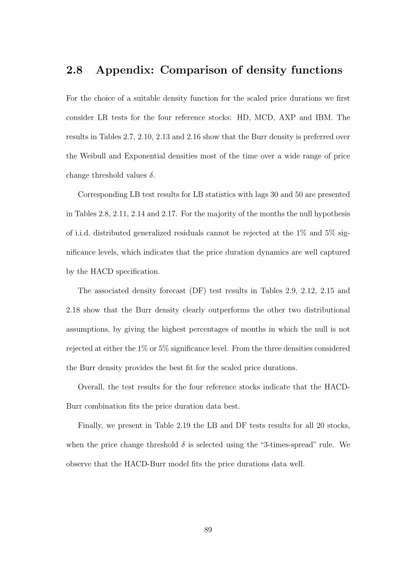
2.8 Appendix: Comparison of density functions
For the choice of a suitable density function for the scaled price durations we first
consider LR tests for the four reference stocks: HD, MCD, AXP and IBM. The
results in Tables 2.7, 2.10, 2.13 and 2.16 show that the Burr density is preferred over
the Weibull and Exponential densities most of the time over a wide range of price
change threshold values δ.
Corresponding LB test results for LB statistics with lags 30 and 50 are presented
in Tables 2.8, 2.11, 2.14 and 2.17. For the majority of the months the null hypothesis
of i.i.d. distributed generalized residuals cannot be rejected at the 1% and 5% sig-
nificance levels, which indicates that the price duration dynamics are well captured
by the HACD specification.
The associated density forecast (DF) test results in Tables 2.9, 2.12, 2.15 and
2.18 show that the Burr density clearly outperforms the other two distributional
assumptions, by giving the highest percentages of months in which the null is not
rejected at either the 1% or 5% significance level. From the three densities considered
the Burr density provides the best fit for the scaled price durations.
Overall, the test results for the four reference stocks indicate that the HACD-
Burr combination fits the price duration data best.
Finally, we present in Table 2.19 the LB and DF tests results for all 20 stocks,
when the price change threshold δ is selected using the “3-times-spread” rule. We
observe that the HACD-Burr model fits the price durations data well.
89
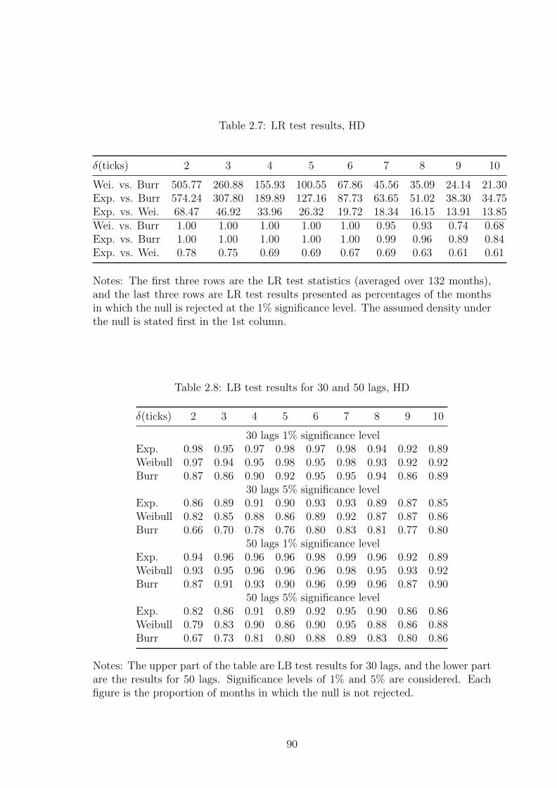
Table 2.7: LR test results, HD
δ(ticks) 2 3 4 5 6 7 8 9 10
Wei. vs. Burr 505.77 260.88 155.93 100.55 67.86 45.56 35.09 24.14 21.30Exp. vs. Burr 574.24 307.80 189.89 127.16 87.73 63.65 51.02 38.30 34.75Exp. vs. Wei. 68.47 46.92 33.96 26.32 19.72 18.34 16.15 13.91 13.85Wei. vs. Burr 1.00 1.00 1.00 1.00 1.00 0.95 0.93 0.74 0.68Exp. vs. Burr 1.00 1.00 1.00 1.00 1.00 0.99 0.96 0.89 0.84Exp. vs. Wei. 0.78 0.75 0.69 0.69 0.67 0.69 0.63 0.61 0.61
Notes: The first three rows are the LR test statistics (averaged over 132 months),and the last three rows are LR test results presented as percentages of the monthsin which the null is rejected at the 1% significance level. The assumed density underthe null is stated first in the 1st column.
Table 2.8: LB test results for 30 and 50 lags, HD
δ(ticks) 2 3 4 5 6 7 8 9 10
30 lags 1% significance levelExp. 0.98 0.95 0.97 0.98 0.97 0.98 0.94 0.92 0.89Weibull 0.97 0.94 0.95 0.98 0.95 0.98 0.93 0.92 0.92Burr 0.87 0.86 0.90 0.92 0.95 0.95 0.94 0.86 0.89
30 lags 5% significance levelExp. 0.86 0.89 0.91 0.90 0.93 0.93 0.89 0.87 0.85Weibull 0.82 0.85 0.88 0.86 0.89 0.92 0.87 0.87 0.86Burr 0.66 0.70 0.78 0.76 0.80 0.83 0.81 0.77 0.80
50 lags 1% significance levelExp. 0.94 0.96 0.96 0.96 0.98 0.99 0.96 0.92 0.89Weibull 0.93 0.95 0.96 0.96 0.96 0.98 0.95 0.93 0.92Burr 0.87 0.91 0.93 0.90 0.96 0.99 0.96 0.87 0.90
50 lags 5% significance levelExp. 0.82 0.86 0.91 0.89 0.92 0.95 0.90 0.86 0.86Weibull 0.79 0.83 0.90 0.86 0.90 0.95 0.88 0.86 0.88Burr 0.67 0.73 0.81 0.80 0.88 0.89 0.83 0.80 0.86
Notes: The upper part of the table are LB test results for 30 lags, and the lower partare the results for 50 lags. Significance levels of 1% and 5% are considered. Eachfigure is the proportion of months in which the null is not rejected.
90
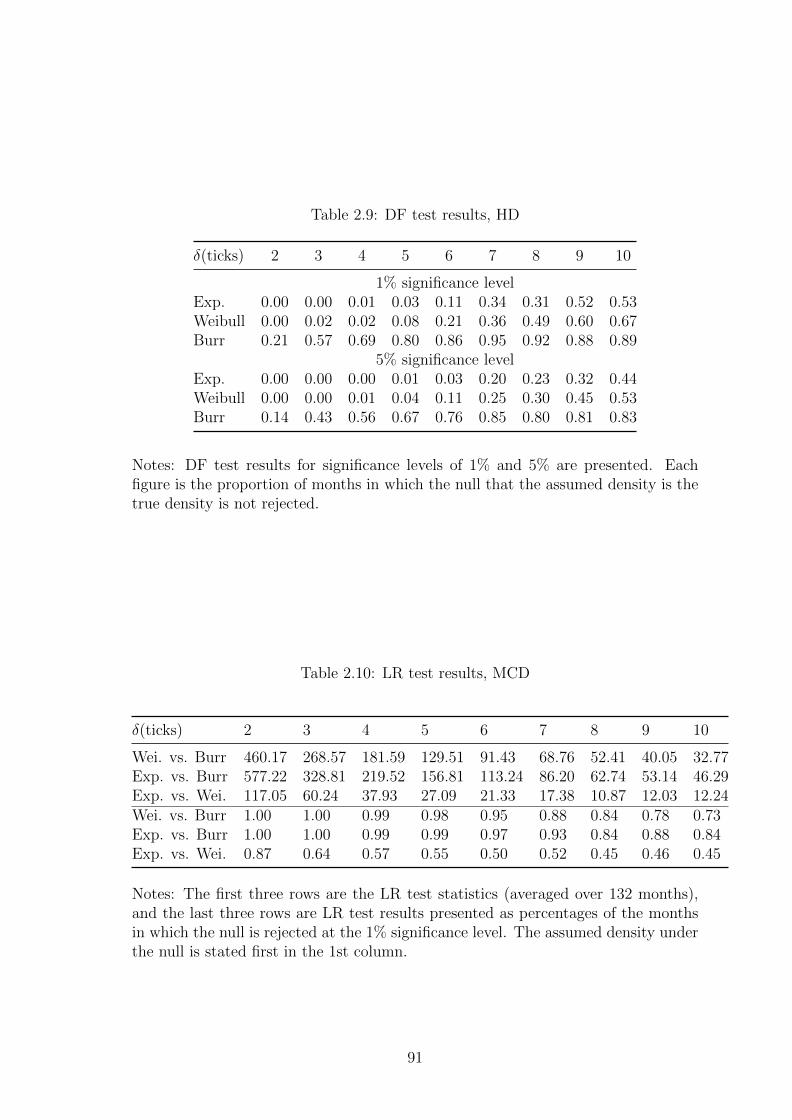
Table 2.9: DF test results, HD
δ(ticks) 2 3 4 5 6 7 8 9 10
1% significance levelExp. 0.00 0.00 0.01 0.03 0.11 0.34 0.31 0.52 0.53Weibull 0.00 0.02 0.02 0.08 0.21 0.36 0.49 0.60 0.67Burr 0.21 0.57 0.69 0.80 0.86 0.95 0.92 0.88 0.89
5% significance levelExp. 0.00 0.00 0.00 0.01 0.03 0.20 0.23 0.32 0.44Weibull 0.00 0.00 0.01 0.04 0.11 0.25 0.30 0.45 0.53Burr 0.14 0.43 0.56 0.67 0.76 0.85 0.80 0.81 0.83
Notes: DF test results for significance levels of 1% and 5% are presented. Eachfigure is the proportion of months in which the null that the assumed density is thetrue density is not rejected.
Table 2.10: LR test results, MCD
δ(ticks) 2 3 4 5 6 7 8 9 10
Wei. vs. Burr 460.17 268.57 181.59 129.51 91.43 68.76 52.41 40.05 32.77Exp. vs. Burr 577.22 328.81 219.52 156.81 113.24 86.20 62.74 53.14 46.29Exp. vs. Wei. 117.05 60.24 37.93 27.09 21.33 17.38 10.87 12.03 12.24Wei. vs. Burr 1.00 1.00 0.99 0.98 0.95 0.88 0.84 0.78 0.73Exp. vs. Burr 1.00 1.00 0.99 0.99 0.97 0.93 0.84 0.88 0.84Exp. vs. Wei. 0.87 0.64 0.57 0.55 0.50 0.52 0.45 0.46 0.45
Notes: The first three rows are the LR test statistics (averaged over 132 months),and the last three rows are LR test results presented as percentages of the monthsin which the null is rejected at the 1% significance level. The assumed density underthe null is stated first in the 1st column.
91
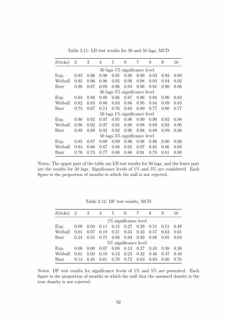
Table 2.11: LB test results for 30 and 50 lags, MCD
δ(ticks) 2 3 4 5 6 7 8 9 10
30 lags 1% significance levelExp. 0.93 0.96 0.98 0.95 0.98 0.99 0.93 0.93 0.89Weibull 0.92 0.96 0.96 0.95 0.98 0.98 0.93 0.94 0.92Burr 0.90 0.87 0.89 0.86 0.94 0.96 0.91 0.90 0.86
30 lags 5% significance levelExp. 0.83 0.86 0.88 0.86 0.87 0.96 0.88 0.90 0.83Weibull 0.82 0.83 0.86 0.83 0.86 0.95 0.84 0.89 0.85Burr 0.73 0.67 0.74 0.76 0.82 0.89 0.77 0.80 0.77
50 lags 1% significance levelExp. 0.90 0.92 0.97 0.95 0.98 0.99 0.90 0.92 0.88Weibull 0.90 0.92 0.97 0.95 0.98 0.98 0.89 0.93 0.90Burr 0.89 0.89 0.92 0.92 0.96 0.98 0.89 0.89 0.86
50 lags 5% significance levelExp. 0.85 0.87 0.88 0.89 0.96 0.98 0.86 0.86 0.86Weibull 0.84 0.86 0.87 0.88 0.92 0.97 0.85 0.86 0.88Burr 0.76 0.73 0.77 0.80 0.86 0.91 0.79 0.81 0.80
Notes: The upper part of the table are LB test results for 30 lags, and the lower partare the results for 50 lags. Significance levels of 1% and 5% are considered. Eachfigure is the proportion of months in which the null is not rejected.
Table 2.12: DF test results, MCD
δ(ticks) 2 3 4 5 6 7 8 9 10
1% significance levelExp. 0.00 0.04 0.11 0.15 0.27 0.39 0.51 0.51 0.48Weibull 0.01 0.07 0.18 0.21 0.34 0.43 0.57 0.63 0.61Burr 0.24 0.55 0.75 0.80 0.83 0.92 0.88 0.85 0.84
5% significance levelExp. 0.00 0.00 0.07 0.08 0.13 0.27 0.43 0.38 0.36Weibull 0.01 0.03 0.10 0.13 0.23 0.32 0.40 0.47 0.48Burr 0.14 0.45 0.61 0.70 0.72 0.83 0.83 0.80 0.76
Notes: DF test results for significance levels of 1% and 5% are presented. Eachfigure is the proportion of months in which the null that the assumed density is thetrue density is not rejected.
92
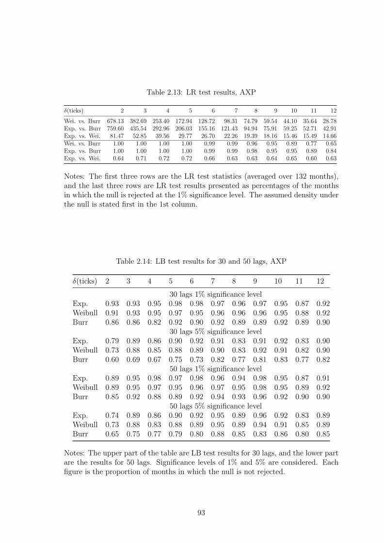
Table 2.13: LR test results, AXP
δ(ticks) 2 3 4 5 6 7 8 9 10 11 12
Wei. vs. Burr 678.13 382.69 253.40 172.94 128.72 98.31 74.79 59.54 44.10 35.64 28.78Exp. vs. Burr 759.60 435.54 292.96 206.03 155.16 121.43 94.94 75.91 59.25 52.71 42.91Exp. vs. Wei. 81.47 52.85 39.56 29.77 26.70 22.26 19.39 18.16 15.46 15.49 14.66Wei. vs. Burr 1.00 1.00 1.00 1.00 0.99 0.99 0.96 0.95 0.89 0.77 0.65Exp. vs. Burr 1.00 1.00 1.00 1.00 0.99 0.99 0.98 0.95 0.95 0.89 0.84Exp. vs. Wei. 0.64 0.71 0.72 0.72 0.66 0.63 0.63 0.64 0.65 0.60 0.63
Notes: The first three rows are the LR test statistics (averaged over 132 months),and the last three rows are LR test results presented as percentages of the monthsin which the null is rejected at the 1% significance level. The assumed density underthe null is stated first in the 1st column.
Table 2.14: LB test results for 30 and 50 lags, AXP
δ(ticks) 2 3 4 5 6 7 8 9 10 11 12
30 lags 1% significance levelExp. 0.93 0.93 0.95 0.98 0.98 0.97 0.96 0.97 0.95 0.87 0.92Weibull 0.91 0.93 0.95 0.97 0.95 0.96 0.96 0.96 0.95 0.88 0.92Burr 0.86 0.86 0.82 0.92 0.90 0.92 0.89 0.89 0.92 0.89 0.90
30 lags 5% significance levelExp. 0.79 0.89 0.86 0.90 0.92 0.91 0.83 0.91 0.92 0.83 0.90Weibull 0.73 0.88 0.85 0.88 0.89 0.90 0.83 0.92 0.91 0.82 0.90Burr 0.60 0.69 0.67 0.75 0.73 0.82 0.77 0.81 0.83 0.77 0.82
50 lags 1% significance levelExp. 0.89 0.95 0.98 0.97 0.98 0.96 0.94 0.98 0.95 0.87 0.91Weibull 0.89 0.95 0.97 0.95 0.96 0.97 0.95 0.98 0.95 0.89 0.92Burr 0.85 0.92 0.88 0.89 0.92 0.94 0.93 0.96 0.92 0.90 0.90
50 lags 5% significance levelExp. 0.74 0.89 0.86 0.90 0.92 0.95 0.89 0.96 0.92 0.83 0.89Weibull 0.73 0.88 0.83 0.88 0.89 0.95 0.89 0.94 0.91 0.85 0.89Burr 0.65 0.75 0.77 0.79 0.80 0.88 0.85 0.83 0.86 0.80 0.85
Notes: The upper part of the table are LB test results for 30 lags, and the lower partare the results for 50 lags. Significance levels of 1% and 5% are considered. Eachfigure is the proportion of months in which the null is not rejected.
93
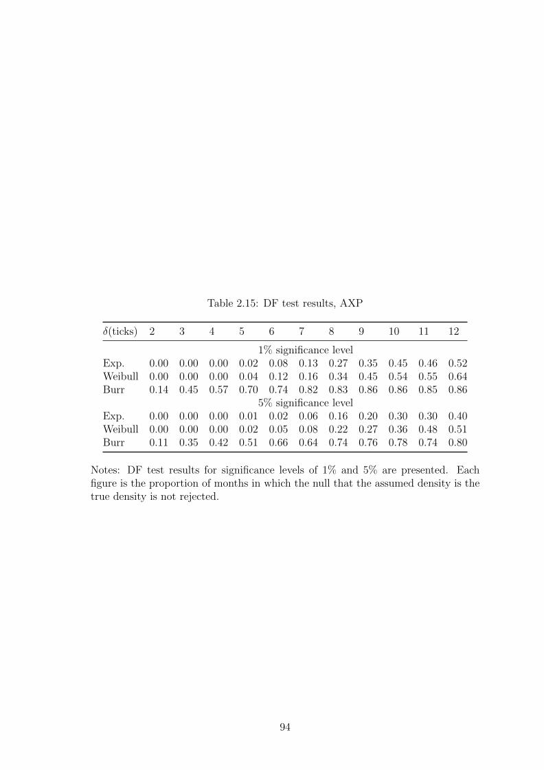
Table 2.15: DF test results, AXP
δ(ticks) 2 3 4 5 6 7 8 9 10 11 12
1% significance levelExp. 0.00 0.00 0.00 0.02 0.08 0.13 0.27 0.35 0.45 0.46 0.52Weibull 0.00 0.00 0.00 0.04 0.12 0.16 0.34 0.45 0.54 0.55 0.64Burr 0.14 0.45 0.57 0.70 0.74 0.82 0.83 0.86 0.86 0.85 0.86
5% significance levelExp. 0.00 0.00 0.00 0.01 0.02 0.06 0.16 0.20 0.30 0.30 0.40Weibull 0.00 0.00 0.00 0.02 0.05 0.08 0.22 0.27 0.36 0.48 0.51Burr 0.11 0.35 0.42 0.51 0.66 0.64 0.74 0.76 0.78 0.74 0.80
Notes: DF test results for significance levels of 1% and 5% are presented. Eachfigure is the proportion of months in which the null that the assumed density is thetrue density is not rejected.
94
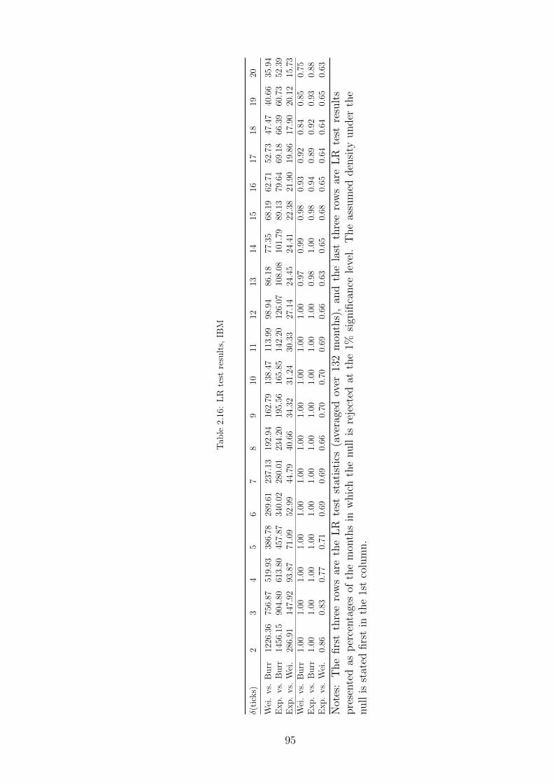
Tab
le2.
16:
LR
test
resu
lts,
IBM
δ(ti
cks)
23
45
67
89
1011
1213
1415
1617
1819
20
Wei
.vs.
Burr
1226
.36
756.
8751
9.93
386.
7828
9.61
237.
1319
2.94
162.
7913
8.47
113.
9998
.94
86.1
877
.35
68.1
962
.71
52.7
347
.47
40.6
635
.94
Exp.
vs.
Burr
1456
.15
904.
8061
3.80
457.
8734
0.02
280.
0123
4.20
195.
5616
5.85
142.
2012
6.07
108.
0810
1.79
89.1
379
.64
69.1
866
.39
60.7
352
.39
Exp.
vs.
Wei
.28
6.91
147.
9293
.87
71.0
952
.99
44.7
940
.66
34.3
231
.24
30.3
327
.14
24.4
524
.41
22.3
821
.90
19.8
617
.90
20.1
215
.73
Wei
.vs.
Burr
1.00
1.00
1.00
1.00
1.00
1.00
1.00
1.00
1.00
1.00
1.00
0.97
0.99
0.98
0.93
0.92
0.84
0.85
0.75
Exp.
vs.
Burr
1.00
1.00
1.00
1.00
1.00
1.00
1.00
1.00
1.00
1.00
1.00
0.98
1.00
0.98
0.94
0.89
0.92
0.93
0.88
Exp.
vs.
Wei
.0.
860.
830.
770.
710.
690.
690.
660.
700.
700.
690.
660.
630.
650.
680.
650.
640.
640.
650.
63
Not
es:
The
firs
tth
ree
row
sar
eth
eL
Rte
stst
atis
tics
(ave
rage
dov
er13
2m
onth
s),
and
the
last
thre
ero
ws
are
LR
test
resu
lts
pre
sente
das
per
centa
ges
ofth
em
onth
sin
whic
hth
enull
isre
ject
edat
the
1%si
gnifi
cance
leve
l.T
he
assu
med
den
sity
under
the
null
isst
ated
firs
tin
the
1st
colu
mn.
95
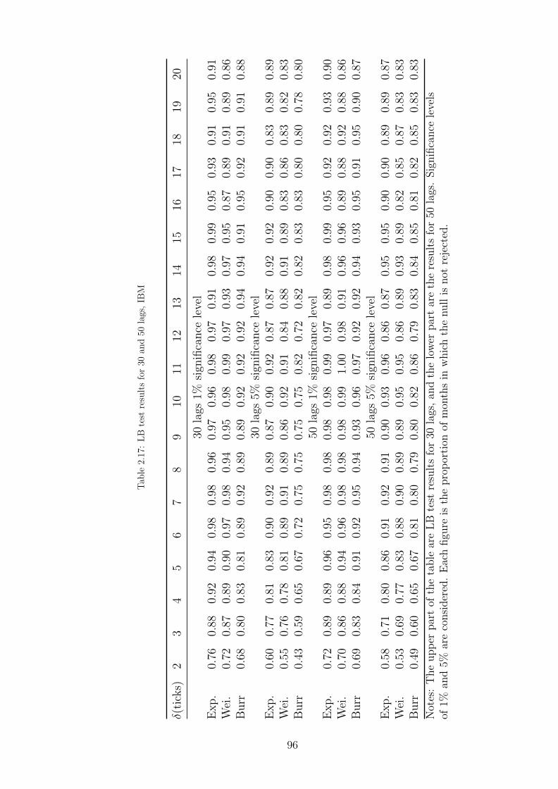
Tab
le2.
17:
LB
test
resu
lts
for
30an
d50
lags
,IB
M
δ(ti
cks)
23
45
67
89
1011
1213
1415
1617
1819
20
30la
gs1%
sign
ifica
nce
leve
lE
xp.
0.76
0.88
0.92
0.94
0.98
0.98
0.96
0.97
0.96
0.98
0.97
0.91
0.98
0.99
0.95
0.93
0.91
0.95
0.91
Wei
.0.
720.
870.
890.
900.
970.
980.
940.
950.
980.
990.
970.
930.
970.
950.
870.
890.
910.
890.
86B
urr
0.68
0.80
0.83
0.81
0.89
0.92
0.89
0.89
0.92
0.92
0.92
0.94
0.94
0.91
0.95
0.92
0.91
0.91
0.88
30la
gs5%
sign
ifica
nce
leve
lE
xp.
0.60
0.77
0.81
0.83
0.90
0.92
0.89
0.87
0.90
0.92
0.87
0.87
0.92
0.92
0.90
0.90
0.83
0.89
0.89
Wei
.0.
550.
760.
780.
810.
890.
910.
890.
860.
920.
910.
840.
880.
910.
890.
830.
860.
830.
820.
83B
urr
0.43
0.59
0.65
0.67
0.72
0.75
0.75
0.75
0.75
0.82
0.72
0.82
0.82
0.83
0.83
0.80
0.80
0.78
0.80
50la
gs1%
sign
ifica
nce
leve
lE
xp.
0.72
0.89
0.89
0.96
0.95
0.98
0.98
0.98
0.98
0.99
0.97
0.89
0.98
0.99
0.95
0.92
0.92
0.93
0.90
Wei
.0.
700.
860.
880.
940.
960.
980.
980.
980.
991.
000.
980.
910.
960.
960.
890.
880.
920.
880.
86B
urr
0.69
0.83
0.84
0.91
0.92
0.95
0.94
0.93
0.96
0.97
0.92
0.92
0.94
0.93
0.95
0.91
0.95
0.90
0.87
50la
gs5%
sign
ifica
nce
leve
lE
xp.
0.58
0.71
0.80
0.86
0.91
0.92
0.91
0.90
0.93
0.96
0.86
0.87
0.95
0.95
0.90
0.90
0.89
0.89
0.87
Wei
.0.
530.
690.
770.
830.
880.
900.
890.
890.
950.
950.
860.
890.
930.
890.
820.
850.
870.
830.
83B
urr
0.49
0.60
0.65
0.67
0.81
0.80
0.79
0.80
0.82
0.86
0.79
0.83
0.84
0.85
0.81
0.82
0.85
0.83
0.83
Not
es:
The
upp
erpar
tof
the
table
are
LB
test
resu
lts
for
30la
gs,
and
the
low
erpar
tar
eth
ere
sult
sfo
r50
lags
.Sig
nifi
cance
leve
lsof
1%an
d5%
are
consi
der
ed.
Eac
hfigu
reis
the
pro
por
tion
ofm
onth
sin
whic
hth
enull
isnot
reje
cted
.
96
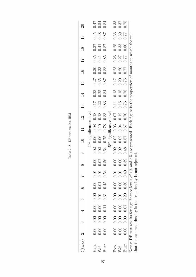
Tab
le2.
18:
DF
test
resu
lts,
IBM
δ(ti
cks)
23
45
67
89
1011
1213
1415
1617
1819
20
1%si
gnifi
cance
leve
lE
xp.
0.00
0.00
0.00
0.00
0.00
0.01
0.00
0.02
0.06
0.08
0.18
0.17
0.23
0.27
0.30
0.35
0.37
0.45
0.47
Wei
.0.
000.
000.
000.
010.
010.
010.
020.
020.
060.
100.
180.
220.
250.
350.
330.
410.
410.
480.
54B
urr
0.00
0.00
0.11
0.31
0.45
0.54
0.56
0.64
0.75
0.78
0.83
0.83
0.84
0.87
0.88
0.85
0.87
0.87
0.84
5%si
gnifi
cance
leve
lE
xp.
0.00
0.00
0.00
0.00
0.00
0.01
0.00
0.02
0.02
0.03
0.07
0.11
0.13
0.17
0.23
0.25
0.25
0.36
0.33
Wei
.0.
000.
000.
000.
010.
000.
010.
000.
020.
020.
040.
120.
160.
150.
200.
200.
270.
330.
390.
37B
urr
0.00
0.00
0.07
0.20
0.30
0.40
0.39
0.48
0.57
0.67
0.70
0.76
0.78
0.75
0.77
0.77
0.80
0.77
0.75
Not
es:
DF
test
resu
lts
for
sign
ifica
nce
leve
lsof
1%an
d5%
are
pre
sente
d.
Eac
hfigu
reis
the
pro
por
tion
ofm
onth
sin
whic
hth
enull
that
the
assu
med
den
sity
isth
etr
ue
den
sity
isnot
reje
cted
.
97
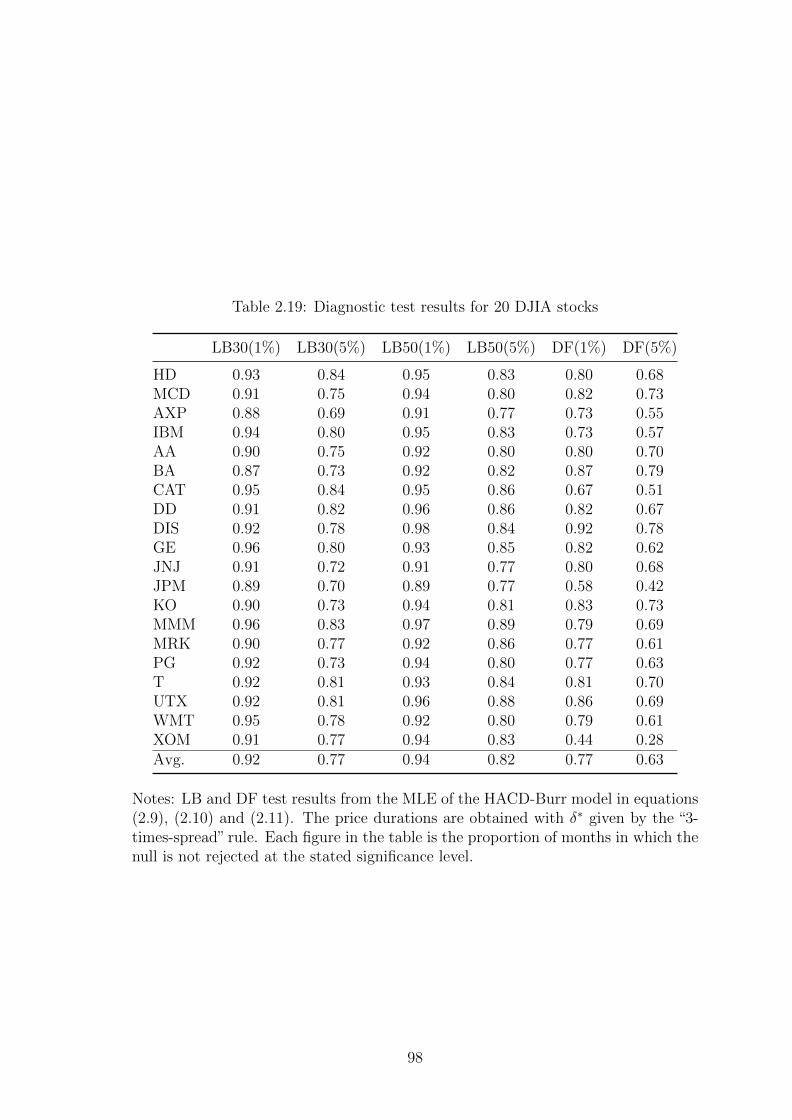
Table 2.19: Diagnostic test results for 20 DJIA stocks
LB30(1%) LB30(5%) LB50(1%) LB50(5%) DF(1%) DF(5%)
HD 0.93 0.84 0.95 0.83 0.80 0.68MCD 0.91 0.75 0.94 0.80 0.82 0.73AXP 0.88 0.69 0.91 0.77 0.73 0.55IBM 0.94 0.80 0.95 0.83 0.73 0.57AA 0.90 0.75 0.92 0.80 0.80 0.70BA 0.87 0.73 0.92 0.82 0.87 0.79CAT 0.95 0.84 0.95 0.86 0.67 0.51DD 0.91 0.82 0.96 0.86 0.82 0.67DIS 0.92 0.78 0.98 0.84 0.92 0.78GE 0.96 0.80 0.93 0.85 0.82 0.62JNJ 0.91 0.72 0.91 0.77 0.80 0.68JPM 0.89 0.70 0.89 0.77 0.58 0.42KO 0.90 0.73 0.94 0.81 0.83 0.73MMM 0.96 0.83 0.97 0.89 0.79 0.69MRK 0.90 0.77 0.92 0.86 0.77 0.61PG 0.92 0.73 0.94 0.80 0.77 0.63T 0.92 0.81 0.93 0.84 0.81 0.70UTX 0.92 0.81 0.96 0.88 0.86 0.69WMT 0.95 0.78 0.92 0.80 0.79 0.61XOM 0.91 0.77 0.94 0.83 0.44 0.28Avg. 0.92 0.77 0.94 0.82 0.77 0.63
Notes: LB and DF test results from the MLE of the HACD-Burr model in equations(2.9), (2.10) and (2.11). The price durations are obtained with δ∗ given by the “3-times-spread” rule. Each figure in the table is the proportion of months in which thenull is not rejected at the stated significance level.
98
Chapter 3
High-frequency covariance matrix
estimation using price durations
99
Abstract
We propose a price duration based covariance estimator using high frequency trans-
actions data. The effect of the last-tick time-synchronisation methodology, together
with effects of important market microstructure components is analysed through a
comprehensive Monte Carlo study. To decrease the number of negative eigenvalues
produced by the non positive-semi-definite (psd) covariance matrix, we devise an
average covariance estimator by taking an average of a wide range of duration based
covariance matrix estimators. Empirically, candidate covariance estimators are im-
plemented on 19 stocks from the DJIA. The duration based covariance estimator is
shown to provide comparably accurate estimates with smaller variation compared
with competing estimators. An out-of-sample GMV portfolio allocation problem is
studied. A simple shrinkage technique is introduced to make the sample matrices
psd and well-conditioned. Compared to competing high-frequency covariance ma-
trix estimators, the duration based estimator is shown to give more stable portfolio
weights over the sample period while maintaining a comparably low portfolio vari-
ance.
Keywords: Price durations; Covariance estimation; High-frequency data; Mar-
ket microstructure noise; Minimum variance portfolio.
100
3.1 Introduction
Asset correlations play a crucial role in many finance applications. Estimation of
a high-dimensional variance-covariance matrix using low frequency data, such as
daily data, typically requires a long time span, making it difficult to catch the most
recent trend in the changes of asset correlations. The advent of tick-by-tick high-
frequency data brings both opportunities and challenges. On the one hand, with
high-frequency data we can greatly shorten the estimation window. On the other
hand, the presence of market microstructure (MMS) noise and non-synchronous
trade arrival times in the high-dimensional setting complicates the implementation
of the standard covariance estimator in calendar time.
In this paper, we propose a high frequency covariance matrix estimator using
price durations. A price duration is defined as the time taken for the absolute cu-
mulative price/return changes to exceed a threshold value. This matrix estimator
takes the average of a range of duration based covariance matrix estimators to gain
efficiency and reduce the number of negative eigenvalues. We show through simu-
lation the effects of MMS noise and the last-tick time-synchronization method on
this duration based covariance estimator. Compared to other candidate covariance
estimators in terms of bias and efficiency, the duration based estimator shows compa-
rable bias but lower standard deviation. In an out-of-sample (OTS) global minimum
variance (GMV) portfolio allocation exercise, the duration based covariance matrix
estimator performs on par with competing estimators in terms of GMV portfolio
variance while yielding considerably lower portfolio weight turnover rates.
In the existing literature, the effect of MMS noise on univariate variance estima-
101
tion has been widely studied. Three main approaches are proposed: the subsampling
approach of Zhang et al. (2005) and Ait-Sahalia et al. (2011), the realised kernel es-
timator of Barndorff-Nielsen et al. (2008a), and the pre-averaging approach of Jacod
et al. (2009).
In the multivariate case, Epps (1979) document the observation that as the sam-
pling frequency of stock returns increases, the corresponding return correlations
have a strong tendency towards zero. Reno (2003) investigate the dynamics un-
derlying the Epps effect and show that this effect can largely be explained by the
non-synchronization of price observations and the consequent lead-lag relationships
between asset prices. Later, different time-synchronization schemes have been pro-
posed, including the last-tick method by Zhang (2011) and the refresh time method
by Barndorff-Nielsen, Hansen, Lunde and Shephard (2011). Hayashi and Yoshida
(2005) (HY) propose the first high frequency covariance estimator that accounts for
the time-synchronization effect by taking the cumulative sum of the cross-product
of all overlapping returns in the absence of noise. To enhance the HY estimator,
Voev and Lunde (2007) propose a procedure to correct for MMS noise bias for the
HY estimator and a subsampling version of the bias-corrected estimator; Griffin and
Oomen (2011) propose a lead-lag adjustment to a sparse sampling implementation
of the HY estimator that is more efficient when the level of MMS noise is high.
As an extension to the three approaches in estimating univariate variances, the
multivariate counterparts are proposed, including the realized kernel (RK) covari-
ance estimator by Barndorff-Nielsen et al. (2011), the two-scale (TS) covariance
estimator by Zhang (2011), and the pre-averaging covariance estimator by Chris-
102
tensen, Kinnebrock and Podolskij (2010). The RK estimator of Barndorff-Nielsen
et al. (2011) is constructed under the Refresh Time sampling scheme, where trade
arrivals of different stocks are synchronised based on the slowest member. This sam-
pling scheme has the drawback that it throws away a significant amount of data
especially when the sample contains some very illiquid stocks. Other estimators are
proposed to make more efficient use of data. Lunde, Shephard and Sheppard (2016)
refine the realized kernel covariance estimator into a composite realized kernel where
univariate realized kernels are used to estimate variances and bivariate realized ker-
nels estimate correlations. Hautsch, Kyj and Oomen (2012) introduce a blocking and
regularization approach where the S&P500 stocks are grouped according to liquidity
so as to reduce data loss. As a frequency domain extension of the RK estimator,
Park, Hong and Linton (2016) propose a Fourier realized kernel covariance estimator
for which no explicit time-alignment is required. Another interesting high-frequency
covariance estimator is the quasi-maximum likelihood estimator of Ait-Sahalia, Fan
and Xiu (2010) that is free of any tuning parameter.
The rest of the paper is organized as follows. Section 3.2 lays out the theoreti-
cal foundation. Section 3.3 summarizes data properties. Section 3.4 shows through
simulation: 1) for one pair of assets, the effects of the last-tick time-synchronization
method and MMS noise on the duration based covariance estimator; 2) for a co-
variance matrix of 19 assets, the negative eigenvalue problem and its mitigation by
taking an average over a wide range of duration based covariance matrix estimators.
Section 3.5 presents empirical comparison of the duration based covariance matrix
estimator with other high-frequency covariance estimators in terms of accuracy and
103
efficiency as well as results on an OTS GMV portfolio allocation problem.
3.2 Theoretical foundation
We will compose the duration based covariance matrix on a pairwise basis. Three
approaches in computing the covariance of a pair of assets using individual variances
are laid out in Section 3.2.1. The non-parametric duration based variance estimator,
NPDV, is used to calculate variances. The derivation of NPDV is in Section 3.2.2.
3.2.1 Three approaches
We will first lay out the three approaches in estimating covariance through variances.
Later through simulation we will show the relative efficiency and bias of the three
approaches.
Assume the two efficient log-price processes, X1t and X2t, are pure diffusion
processes with no drift. The weighted sum of the two diffusion processes follows:
d(X1t + θX2t) = σX1tdB1t + θσX2tdB2t, (3.1)
where θ is a weighting parameter. For the two Brownian processes, dB1t ·dB2t = ρtdt.
From now on we keep σt and ρt constant through the estimation interval, usually
one trading day, so we drop the subscript t. Let X(θ) = X1 + θX2 and σ2X(θ) denote
the variance of the above process, then
σ2X(θ) = σ2
X1 + θ2σ2X2 + 2θρσX1σX2 . (3.2)
104
When θ = 1, σ2X(θ) = σ2
(X1+X2), and we have:
σ2(X1+X2) = σ2
X1 + σ2X2 + 2ρσX1σX2 . (3.3)
When θ = −1, σ2X(θ) = σ2
(X1−X2), and we have:
σ2(X1−X2) = σ2
X1 + σ2X2 − 2ρσX1σX2 . (3.4)
Let V ar(·) denote the estimate of σ2(·), Cov(X1, X2) the estimate of ρσX1σX2 .
Then from equations (3.3) and (3.4), we have three methods to calculate Cov(X1, X2):
Cov1(X1, X2) = 12(V ar(X1 +X2)− V ar(X1)− V ar(X2)); (3.5)
Cov2(X1, X2) = 12(V ar(X1) + V ar(X2)− V ar(X1 −X2)); (3.6)
Cov3(X1, X2) = 14(V ar(X1 +X2) + V ar(X1 −X2)). (3.7)
Note that Cov3(X1, X2) = 12(Cov1(X1, X2) + Cov2(X1, X2)). V ar(·) will be cal-
culated using the non-parametric duration-based variance estimator, NPDV (or
NP ), as derived below.
3.2.2 NPDV
The derivation of the univariate non-parametric duration based variance estimator,
NPDV, is exactly the same as in Chapter 2 and Nolte, Taylor and Zhao (2016).
Initially we assume that the univariate efficient log-price, Xt, follows a pure
105
diffusion process with no drift, represented by
dXt = σX,tdBt. (3.8)
For each trading day and a selected threshold δ, a set of event times td, d =
0, 1, ... is defined in terms of absolute cumulative log-price changes exceeding δ, by
t0 = 0 and
td = inft>td−1
|Xt −Xtd−1| = δ, d ≥ 1. (3.9)
Let xd = td − td−1 denote the time duration between consecutive events and let
Id−1 denote the complete price history up to time td−1. For the conditional distri-
bution xd|Id−1, we denote the density function by f(xd|Id−1), the cumulative den-
sity function by F (xd|Id−1) and the intensity (or hazard) function by λ(xd|Id−1) =
f(xd|Id−1)/(1− F (xd|Id−1)).
Following Engle and Russell (1998) and Tse and Yang (2012), duration based
variance estimators rely on a relationship between the conditional intensity function
and the conditional instantaneous variance of a step process. The step process
Xt, t ≥ 0 is defined by Xt = Xt when t ∈ td, d ≥ 0 and by Xt = Xtd−1 whenever
td−1 < t < td. The conditional instantaneous variance of Xt equals
σ2X,t = lim
∆→0
1∆ var(Xt+∆ − Xt|Id−1), td−1 < t < td. (3.10)
As ∆ approaches zero we may ignore the possibility of two or more events between
times t and t+ ∆, so that the only possible outcomes for Xt+∆− Xt can be assumed
106
to be 0, δ and −δ. The probability of a non-zero outcome is determined by λ(x|Id−1)
and consequently
σ2X,t = δ2λ(t− td−1|Id−1), td−1 < t < td. (3.11)
The integral of σ2X,t
over a fixed time interval provides an approximation to the
integral of σ2X,t over the same time interval, and the approximation error disappears
as δ → 0.
Let there be N price duration times during a day, then the general duration
based estimator of integrated variance, IV , is given by
IV =tN∫0
σ2X,tdt =
N∑d=1
δ2td∫
td−1
λ(t− td−1|Id−1)dt
= −δ2N∑d=1
ln(1− F (xd|Id−1)). (3.12)
In practice, we do not know the true intensity function. We must therefore either
estimate the functions λ(.|.) or we can replace the summed integrals in (3.12) by their
expectations. As these expectations are always one, the non-parametric, duration
based variance estimator, NPDV , is simply
NPDV = Nδ2. (3.13)
This equals the quadratic variation of the approximating step process over a
single day, which we may hope is a good estimate of the quadratic variation of the
diffusion process over the same time interval. An equation like (3.13), for the special
107
case of constant volatility, can be found in the early investigation of duration based
methods by Cho and Frees (1988).
Note that δ is the threshold value for returns. So V ar(X1+X2) and V ar(X1−X2)
should be calculated by adding up synchronized returns (not price changes) from the
processes X1t ± X2t. The selection of δ, as a return measure, for the estimation of
V ar(X1(2)) and V ar(X1 ±X2), is in Section 3.4.1.3.
3.3 Data properties
In the empirical analysis we use 19 of the 30 stocks of the Dow Jones Industrial
Average (DJIA) index; these are the 20 stocks studied in Chapter 2 except stock
T is excluded. 1 The tick-by-tick trades and quotes data spanning 11 years (2769
tading days) from January 2002 to December 2012 are obtained from the New York
Stock Exchange (NYSE) TAQ database and are time-stamped to a second. The
stocks selected have their primary listing at NYSE without interruption during the
sample period.
The raw data is cleaned using the method of Barndorff-Nielsen et al. (2009). Data
entries that meet one or more of the following conditions are deleted: 1) entries out
of the normal 9:30am to 4pm daily trading session; 2) entries with either bid, ask
or transaction price equal to zero; 3) transaction prices that are above the ask price
plus the bid/ask spread or below the bid price minus the bid/ask spread; 4) entries
with negative bid/ask spread; 5) entries with spread larger than 50 times the median
1From the list of 30 DJIA stocks as of December 2012, CSCO, INTC, and MSFT are excludedas their primary listing is at NASDAQ; BAC, CVX, HPQ, PFE, TRV, UNH, and VZ are excludedbecause of incomplete NYSE data samples; T is excluded because of the loss of one trading daydue to corporate merger.
108
spread of the day. When multiple transaction, bid or ask prices have the same time
stamp, the median price is used.
For our analysis we merge the individual trades and quotes files using a refined
Lee and Ready algorithm as outlined in Nolte (2008) to identify trades with corre-
sponding bid and ask quotes, which yields associated buy and sell indicators as well
as bid/ask spreads.
The list of stocks and descriptive statistics for the whole sample period are pre-
sented in Table 3.1, which repeats the information in Table 2.1 in Chapter 2. Table
3.1 shows means and medians for bid/ask spreads and inter-trade durations, as well
as means for the price levels and volatilities for all stocks, sorted in the ascending
order of their mean spread level in the first column. The mean values of bid/ask
spreads range from 1.4 to 3.5 cents, and from 3.55 to 7.01 seconds for trade du-
rations. The corresponding medians range from 1 to 2 cents, and 2 to 3 seconds,
respectively, implying right-skewed distributions for both variables. Table 3.1 also
presents means and medians for a simple measure of a jump frequency. A jump is
recorded when the absolute value of a price change exceeds five times the average
bid/ask spread for a given day. Both mean and median values indicate that there
are about 1 to 2 of these jump events on average per day.
We also observe that the average level of volatility across the whole sample period
lies between 15% and 31%, while the average price level ranges from $26 to $108.
We clearly observe that the average bid/ask spread is increasing with the average
price level.
Table 3.2 presents the correlations of returns and trade arrivals for the 19 stocks.
109
In the upper triangle are the correlations of returns and the lower triangle contains
the correlations of trade arrivals. Returns are calculated on 30min intervals. Corre-
lation of trade arrivals is calculated as the correlation between the numbers of trade
arrivals within a specified time bin, for example 40 seconds. We count the numbers
of trade arrivals within each of the 585 40sec bins every day for all 19 stocks. We
then calculate the correlations of the counts in each 40sec bin for each pair of stocks.
In the lower triangle of Table 3.2 are the trade arrival correlations averaged over
the 585 bins for the 171 pairs of stocks. In the last column are average 30min return
correlations of one stock with the other 18 stocks, and in the last row are corre-
sponding average 40sec trade arrival correlations. The average correlation between
returns is around 0.5, and the average correlation between trade arrivals is around
0.4.
Figure 3.1 plots the trade arrival correlations averaged over the 171 pairs for
the 585 40sec bins over the daily trading session from 9:30 to 16:00. The three
“jump” points are highlighted. They occur at 10:00, 14:00, and 15:40. The first two
correlation jumps can be explained by regular U.S. economic news announcements
at 10am and 2pm. The third jump at 15:40 is due to NYSE’s requirement that
orders which are not entered to offset a published order imbalance must be entered
by 15:40 EST to be executed at the close of a market.
We can also see an increased average trade arrival correlation over the last one-
third of the daily trading session, which may be due to more active trading as the
market is nearer to closing.
110
3.4 Simulation results
We perform two types of simulations in this section. The first simulation is done
on one pair of assets with 2000 replications, and the second simulation done on a
covariance matrix of 19 assets with 100 replications. Each replication is a simulation
for one trading day. The aim of the first simulation is to compare the performance
of the covariance estimates using the three duration based covariance estimation
methods in Section 3.2 with other popular covariance estimators, and to study the
effect of time-synchronization and bid/ask spread on the estimation of V ar(X1±X2).
We study the effect of the last-tick time-synchronization method by varying the
correlation of trade arrivals, ρarr. We consider three levels of trade arrival correlation:
ρarr = 0, ρarr = 1, and ρarr = 0.4, all explained in more detail later. Other parameter
values are set to be consistent with empirical data properties: ρ = 0.5, σX1 = σX2 =
0.25, and initial price P0 = 50. In this setup, σ2(X1−X2) = σ2
X1 = σ2X2 = 1
3σ2(X1+X2).
The aim of the second simulation is to assess the performance of the duration
based covariance estimator in a matrix setup, consisting of 19 stocks, in order to
study its property of positive semi-definiteness (psd). The starting prices, volatilities,
trade durations, and spread levels of the 19 stocks are set as the average values as
shown in Table 3.1. The correlations of individual stock returns are set as shown in
Table 3.2. Trade arrivals are assumed to be independent in this matrix setup.
111
3.4.1 Simulation on one pair of assets
3.4.1.1 Time-synchronization effect
The time-synchronization issue stems from the fact that trades occur at discrete
and different times for different stocks, so we first need to discretize the diffusion
process for each log-price. Let ∆1 and ∆2 be the discretization time intervals, and
Y1,i and Y2,j be the noisy trade (log-)prices, where i(j) = 0, . . . , I(J), I and J
being the number of trades during the daily trading session for asset 1 and 2. Y1,i
and Y2,j consist of discretized efficient (log-)price processes X1,i and X2,j and noise
components.
Discretizing X1t and X2t yields time-discretized diffusion components
X1t −X1,t−∆1 = σX1
√∆Z1t; (3.14)
X2t −X2,t−∆2 = σX2
√∆Z2t. (3.15)
Here, Z1t and Z2t are standard normally distributed random variables with cor-
relation ρ = 0.5 and σX1 and σX2 are the daily integrated volatilities, which are
assumed to be constant.
In implementation, we first draw 23,400 (since there are 23,400 seconds per trad-
ing day) equally spaced efficient return points using equations (3.14) and (3.15) with
∆ = 1 second, and then select the points where trades occur with random Bernoulli
trials of probability 1/∆1 or 1/∆2. In this section, we set ∆1 = ∆2 = 6 seconds. We
convert cumulative returns into prices based on an initial price of P0 = 50. Finally,
112
we can add bid/ask spreads as described in Section 3.4.1.2.
We synchronize two discretized processes using the last-tick synchronization
method, that is, we retain all trades of the two series, and when only one asset
trades at a transaction time t1,i or t2,j we interpolate by adding in the last trade
price of the no-trade asset.
To investigate the effect of the last-tick time-synchronization method on the NP
estimates of V ar(X1 +X2) and V ar(X1−X2), we consider three levels of correlation
between trade arrivals, ρarr: 1) identical trade arrivals, ρarr = 1, where the trade
times of the two assets are the same; 2) independent trade arrivals, ρarr = 0, where
two trade times are generated independently; 3) correlated trade arrivals, ρarr = 0.4,
and the construction of two correlated Bernoulli processes is in the Appendix. The
third scenario conforms to the real data.
Figure 3.2 plots the NP estimates of V ar(·) when the trade arrival times of
the two time-discretized processes are the same, ρarr = 1, so that we do not need
to synchronize the trades. The return thresholds are calculated using the thresh-
old number of ticks on the x-axis divided by P0. Due to time-discretization, the
ratios of V ar(·) over σ2(·) do not reach unity but are increasing as the threshold
value increases.2 V ar(X1 − X2), V ar(X1), and V ar(X2) give the same estimates.
V ar(X1 + X2) is converging to the true value slower than the other three, because
σ2(X1+X2) is three times the value of σ2
(X1−X2) and needs a larger threshold to mitigate
the time-discretization effect.
2The time-discretization noise stems from the fact that trades do not arrive continuously. Here,time-discretization decreases the number of events observed, due to the absence of price pointsthat may have defined price events. Increasing the threshold value reduces the bias introduced bytime-discretization.
113
In Figure 3.3, we let the two series of trade arrival times be independent, so
ρarr = 0. We observe that, compared to Figure 3.2, V ar(X1−X2) estimates increase
significantly. This is due to what we call the “reverse Epps” effect.
The Epps and reverse Epps effects arise when we estimate V ar(X1 ±X2) using
the last-tick synchronization method. They exist whenever ρ 6= 0 and ρarr 6= 1.
When ρ > 0, the (latent) returns of the two assets over an interval ∆, R1,∆ and R2,∆
are more likely to be of the same sign. Assume only asset 1 has a trade at the end
of this ∆ time interval, when we synchronize the arrival times by plugging in the
last trade price of asset 2, this stagnant price would reduce R2,∆ to zero. |R1 + R2|
is decreased, so does V ar(X1 + X2), rendering the Epps effect; while |R1 − R2| is
increased, so does V ar(X1 −X2), rendering the reverse Epps effect. No such effects
exist when ρ = 0.
So due to the Epps effect, we would expect V ar(X1+X2) estimates to decrease in
Figure 3.3 compared to those in Figure 3.2, but it does not seem so. This is due to the
decreased time-discretization effect, which arises whenever ρarr 6= 1. The last-tick
interpolation method is increasing the number of trades for both series, rendering
the synchronized process finer discretized than both individual series, thus increasing
the NP estimates of both V ar(X1 +X2) and V ar(X1 −X2).
In Figure 3.4, we plot the more realistic scenario, where ρarr = 0.4. We see that
the effects from last-tick time-synchronization are less pronounced than the case
when ρarr = 0, but still quite significant compared to the case with identical trade
arrivals.
114
3.4.1.2 Bid/ask spread effect
In this section we briefly discuss the effect of bid/ask spread on the estimation of
V ar(X1±X2), which is similar to the bid/ask spread effect discussed in Nolte et al.
(2016) on the estimation of V ar(X1(2)).
Bid and ask transaction prices are generated by Yi(j) = Xi(j) +0.51i(j)s1(2), where
s1(2) is the bid/ask spread for asset 1(2), which is assumed to be constant. 1i(j) is
an indicator variable which equals 1 when Yi(j) represents an ask price and -1 when
Yi(j) represents a bid price. The transaction price takes either the bid or the ask side
with probability 0.5 and the variables 1i(j) are i.i.d.
In Figure 3.5, we add bid/ask spread, s1 = s2 = 2 ticks, to both series of
transaction prices with correlated trade arrival times. As expected, the bid/ask
spread increases all V ar(·) estimates.
3.4.1.3 Compare the three Cov estimation methods
As seen in equations (3.5), (3.6), and (3.7), there are three ways to calculate Cov(X1, X2)
using V ar(X1 ± X2), V ar(X1), and V ar(X2). Now that we have seen the effects
of time-discretization, time-synchronization, and bid/ask spread on the individual
components, in this section we will put them together and compare the performance
of the three methods in terms of bias and efficiency over a range of threshold values.
We will also compare the duration based covariance estimators with other popular
covariance estimators, including the realized kernel (RK), two-scaled (TS), 5min,
and 30min realised covariance (RC) estimators.
RK and TS estimators in this section and in the empirical section are constructed
115
following the same rules. RK is constructed conforming to Barndorff-Nielsen et al.
(2011). The Parzen kernel is used, with c∗ = 3.51. For the estimation of the optimal
bandwidth H∗, the 10min sub-sampled RV is used to approximate the square-root of
integrated quarticity and the 30sec sub-sampled RV used to approximate the noise
variance. TS is constructed as in Zhang (2011). The fast scale is 10 seconds and the
slow scale is 5 minutes.
In addition to the scenario in the last section (scenario 3 in Table 3.3), we add
two other scenarios. Scenario 1 has ∆1 = 2 seconds, ∆2 = 4 seconds, s1 = 1 ticks,
s2 = 1.5 ticks; and scenario 2 has ∆1 = 4 seconds, ∆2 = 8 seconds, s1 = 1.5 ticks,
s2 = 3 ticks. In Figures 3.6, 3.7 and 3.8 we plot the ratios of the duration based
covariance estimates over the true value against the threshold number of multiples
of the spread on the x-axis for the three scenarios; the standard deviations (STDs)
of the duration based covariance estimates are in Figures 3.9, 3.10 and 3.11, and the
RMSE’s of the estimates are plotted in Figures 3.12, 3.13 and 3.14.
Note that on the x-axis of Figures 3.6 to 3.14 it is no longer the number of ticks
but the number of multiples of the spread for the threshold, since we want to add
a “staggering feature” to V ar(X1(2)) and V ar(X1 ± X2) so that they don’t share
the same threshold value. The threshold number of ticks for the variance estimate
of a single stock is still set as a range of multiples of the spread of this stock, so
s = s1(2) for V ar(X1(2)). But the threshold for the variance estimate of the portfolio
of two stocks is set as a range of multiples of the sum of the spread of the two
stocks, so s = s1 + s2 for V ar(X1 ±X2), because s1 + s2 is the spread for X1 ±X2.
V ar(X1 +X2) and V ar(X1−X2) use the same threshold because we assume in the
116
simulation that trades take the bid or the ask side at random. The staggering feature
here allows us to put a larger threshold value on V ar(X1 ±X2), which is desirable,
since V ar(X1 ± X2) are converging slower to the true values than V ar(X1(2)), as
seen in Figure 3.5.
In terms of bias, as seen in Figures 3.6, 3.7, and 3.8, Cov1 is the least biased
in all three scenarios but, as shown in Figures 3.9, 3.10, and 3.11, it also has the
largest STD among the three methods. The bias of the estimates decreases while
the standard deviation increases as the threshold increases. The RMSE takes into
account the effects of both bias and STD so that the U-shape curves are evident
for all three estimators, as shown in Figures 3.12, 3.13, and 3.14. Roughly between
thresholds of 2 to 6 times the spread the RMSE’s are relatively stable. Cov1 shows
lower RMSE on the lower end of the threshold than Cov2 and Cov3 in all three
scenarios.
The reason why Cov1 is the least biased can be found in Figure 3.5, which shows
a realistic scenario with bid/ask spread as well as correlated trade arrivals. Due to
the “reverse Epps” effect, V ar(X1−X2) is greatly inflated, rendering Cov2 and Cov3
estimates to be smaller and more biased. The most biased among the three is Cov2.
This is because in the calculation of Cov2, V ar(X1(2)) uses smaller threshold values
than V ar(X1 −X2), which makes their difference larger. While V ar(X1 −X2) and
V ar(X1 + X2) share the larger threshold value so that they are both less biased,
which makes Cov3 more accurate than Cov2.
To look more closely, we tabulate in Table 3.3 the Bias, Standard Deviation
(STD) and RMSE statistics for the three methods using price durations over thresh-
117
old number of multiples from 1 to 5 times the spread, together with the same statis-
tics for the RK, TS, 5min and 30min realized covariance estimators, for the three
scenarios. Compared to the competing covariance estimators, the duration based
estimates tend to exhibit lower standard deviation but larger bias. The RMSE takes
into account the bias-efficiency tradeoff. Along this dimension, when we choose an
appropriate threshold value, for example 2 to 3.5 times the spread, Cov1 performs
better than the TS, 5min, and 30min realised covariance estimators, and comparable
to the RK estimator. We will use Cov1 to calculate the duration based covariance
estimates from now on and denote it as COV .
3.4.2 Simulation of the covariance matrix
Now we construct the covariance matrix of 19 stocks using COV , the RK and the TS
covariance estimators. The multivariate standard normally distributed variables, Zit
in equations (3.14) and (3.15), with a correlation matrix as in Table 3.2, are generated
using the Eigenvector decomposition, also known as the Spectral Decomposition,
approach. We set ρarr = 0 in this section, so the trade times are independent. All
covariance matrix estimators are constructed on a pairwise basis so the resulting
covariance matrix is not guaranteed to be positive semi-definite. The “Neg Eig”
column of Table 3.4 presents the average number of negative eigenvalues per day.
In the first row, when δ = 3s, the average number of negative eigenvalues per day
is 4.72, but after we average the estimates at δ = 2.5s and δ = 4s, this number
drops to 3.55. When we further take the average over 16 estimates from δ = 2.5s
to δ = 4s with increment 0.1s, the resulting average number of negative eigenvalues
118
drops significantly to 0.22.
Taking the average of the duration based variance-covariance estimates over a
range of threshold values helps improve efficiency, reduce noise and thus decrease the
number of negative eigenvalues per day. Over the range of δ from 2.5s to 4s, when
we decrease the step size to 0.01s, that is to take the average over 151 estimates, the
average number of negative eigenvalues per day drops to 0.01. The same pattern
follows for the threshold range of 2s to 6s. When we move the δ range to the far right
and set the threshold to be very large, there is significant efficiency loss, since the
number of duration observations per day decreases sharply, resulting in significantly
larger number of negative eigenvalues per day compared to the average duration
based estimates with the same step size.
Table 3.4 displays the efficiency and accuracy of different estimators separately
for the diagonal elements, variance, and the off-diagonal elements, covariance. On
the variance part, we see that the duration based estimates are more biased than the
RK and TS estimates, and averaging over a range of threshold values doesn’t seem
to help much in reducing the bias. Only when we increase the threshold values, for
example compare the range of 2.5s to 4s to the range of 7s and 8s, can we reduce
bias, but at the same time the efficiency loss due to decreased number of duration
observations is large. On the other hand, the duration based variance estimates tend
to be less dispersed than the two competing estimators, showing smaller STD, but
when we set the threshold to be extremely large, the STD becomes larger, signalling
a loss of efficiency.
On the covariance part, the duration based estimates show better performance.
119
The bias of the duration based covariance estimates is on average larger than that of
RK but smaller than that of TS. The STD of the duration based covariance estimates
is generally smaller, apart from extreme large threshold cases. Comparing to the
bias of the variance estimates, the reduction in the bias of covariance estimates
(given correlation is approximately 0.5, covariance is roughly half of variance) is
larger in magnitude for COV than for RK and TS. This is because the biases of
V ar(X1 +X2), V ar(X1), and V ar(X2) partially cancel out when estimating COV .
Given comparable bias and smaller STD, the duration based covariance estimates
generally perform better than RK and TS along the RMSE dimension.
Seeing that averaging the duration based estimators helps to reduce the number
of negative eigenvalues per day and to improve efficiency, we will use the average
duration based variance and covariance estimates (still denoted as COV ) in the
empirical study.
3.5 Empirical study
3.5.1 Comparison among candidate covariance matrix esti-
mators
In this section, we construct the covariance matrices of 19 stocks for each of the
2769 trading days using the duration based, RK, and TS methods and compare
them with the 5min, 30min, and open-to-close (OtoC) daily realized covariance
matrix estimates. Two duration based variance/covariance estimators are included:
COV1, which is the average of 401 estimates using price durations based on threshold
120
values from 2 times the daily average spread to 6 times the spread with increment
0.01 times the spread; and COV2, which is the average of 151 estimates using price
durations based on threshold values from 2.5 times the daily average spread to 4
times the spread with increment 0.01 times the spread.
Table 3.5 presents the benchmark 5min and 30min realised variance/covariance
estimates averaged over all trading days, where in the upper diagonal are the aver-
age 5min realised covariances and in the lower diagonal the average 30min realised
covariances.3 The diagonal elements are average realised variance estimates based
on 5min returns and are in italics. Table 3.10 presents the benchmark average OtoC
realised covariance estimates and the diagonal average realised variance estimates
are in italics.
In Tables 3.6 and 3.7, the average daily estimates from COV1, COV2, RK and
TS are compared with the average daily 5min realised variance/covariance estimates.
COV1 estimates are in the upper diagonal, COV2 in the lower and the main diag-
onal. In Table 3.7, RK estimates are in the upper and main diagonal and the TS
estimates in the lower diagonal. Elements that are significantly4 different from the
5min realised variance/covariance benchmark are in bold. Overall, the duration
based estimates are more close to the 5min estimates than RK but less close than
TS, which is shown explicitly in Table 3.13.
In Tables 3.8 and 3.9, we compare COV1, COV2, RK, and TS estimates with
the 30min realised variance/covariance estimates. The duration based estimators
3For illustration purpose, Tables 3.5 to 3.12 present covariance matrices for the first 15 stocksonly, due to limitation of space. Tables 3.13, 3.14, and 3.15 present statistics based on all 19 stocks.
4All significance tests in this section are Newey-West type HAC tests with 1% significance level,as in Barndorff-Nielsen et al. (2011).
121
produce estimates that are closer to the 30min benchmark than both the RK and
TS estimators, as shown explicitly in Table 3.13.
Finally, in Tables 3.11 and 3.12, the four candidate estimates are compared with
the OtoC realised variance/covariance estimates as a benchmark. Both RK and
TS estimates are less different from the OtoC estimates than the duration based
estimates, as shown explicitly in Table 3.13.
Table 3.13 summarizes the comparison between the candidate group including
COV1, COV2, RK, and TS estimators and the benchmark group including the 5min,
30min, and OtoC realised variance/covariance estimators. Results are presented as
the proportion of the matrix elements that are significantly different at 1% signifi-
cance level (using Newey-West type HAC significance test) for the pair of estimators
in comparison. Comparisons are done respectively on the whole matrix, on the off-
diagonal elements, and on the main diagonal elements. On the variance part, the
duration based estimates are closer to the 30min and OtoC estimates than RK and
TS, but less close to the 5min estimates. On the covariance part, the candidate es-
timators generally show lower levels of difference to the benchmark estimators than
on the variance part. Specifically, duration based covariances are more similar to
the 5min estimates than RK but less so than TS; they are also more close to the
30min estimates but less close to the OtoC covariances than RK and TS estimates.
Table 3.14 presents summary statistics including mean, standard deviation and
the first order autocorrelation for the four candidate variance/covariance estimators
and the three benchmarks. The statistics are again presented for the whole ma-
trix, and also separately for the variance and covariance parts. The overall mean
122
estimates of the four candidate estimators are quite close, with RK slightly higher.
The mean variance estimates from the two duration based estimators are lower than
those from the RK and TS estimators, while the mean covariance estimates from
the four candidate estimators are quite close. For the variation of the estimates,
both the variance and covariance estimates from the duration based estimators give
smaller STD than those from the RK and TS estimators. The mean and stan-
dard deviation features of the duration based estimates as compared to the RK and
TS estimates are consistent with the findings from the simulation study in Section
3.4: the duration based covariance estimates exhibit variation smaller than and bias
comparable with the competing estimates. It is also interesting to note that the
duration based variance/covariance estimates have higher first order autocorrelation
than other estimators.
Table 3.15 presents the average correlations between the candidate variance/covariance
estimators and the benchmark estimators. As expected, the four high-frequency
variance/covariance estimators are the most correlated with the 5min realised vari-
ance/covariance estimates, followed by the 30min estimates, and the least correlated
with the daily OtoC realised variance/covariance estimates. The levels of correlations
with the benchmark estimates are very close among the four candidate estimators,
with the duration based estimators showing slightly higher correlations.
3.5.2 A portfolio allocation problem
In this section we compare the global minimum variance (GMV) portfolio allocation
results, evaluated for the one-day ahead 5min portfolio variance. We first calculate
123
the GMV portfolio weights based on the covariance matrices estimated from one
of the four candidate estimators: COV , RK, TS, and sub5min, and then use the
weights to calculate the one-day ahead 5min portfolio variances. Note that in this
section the duration based covariance matrix estimator COV is the COV1 from
Section 3.5.1. Also, sub5min is the sub-sampled 5min realised covariance matrix
estimator.
We will also compare the GMV portfolio variances with the risk parity portfolio
variances and the equal-weight portfolio variances, as is done in Lunde et al. (2016).
Compared to the calculation of GMV portfolio weights which involves all elements
of the matrix, the calculation of risk-parity portfolio weights is based entirely on
the diagonal variance elements of the variance-covariance matrix. Let Ωt denote
the variance-covariance matrix, with dimension p, from one of the four candidate
estimators. The p by 1 vector of GMV portfolio weights, wmt , is calculated as:
wmt = (Ω−1t ι)/(ι′Ω−1
t ι), (3.16)
where ι is a conformable vector of 1’s.
The risk parity portfolio weights, wrt , are inversely proportional to individual
asset variances:
wrt = 1/ diag(Ωt)ι′(1/ diag(Ωt))
, (3.17)
where diag(·) denotes the diagonal of a matrix and 1/ diag(·) is a vector whose
components are the reciprocals of the diagonal terms. The asset weight in an equal-
weight portfolio is 1/p. wmt and wrt are calculated at day t and applied to the 5min
124
portfolio variance at day t+ 1.
3.5.2.1 Eigenvalue cleaning and shrinkage methods
The calculation of wmt requires Ωt to be positive semi-definite (psd). Among the
four candidate covariance estimators, TS and sub5min are guaranteed to be psd.
As for RK and COV , since they are estimated on a pairwise basis, the resulting
matrices are not guaranteed to be psd. A well-functioning covariance matrix should
also be well-conditioned, where the smallest eigenvalue should not vanish to zero on
any trading day of the sample period. Let η denote the ratio of largest/smallest
eigenvalue of a well-conditioned covariance matrix. It represents the tightness of
the 19 eigenvalues. The more spreadout are the eigenvalues, the more “unstable”
the matrix tend to be when being inverted. Hautsch et al. (2012) suggest a well-
conditioned covariance matrix should have η ≤ 10p. Let ηu denote the upper bound
of η, then in our case p = 19 and ηu = 190. Later we will try different values of ηu
to check the robustness of the results.
In the existing literature, there are different eigenvalue cleaning techniques to
convert non-psd covariance matrices into psd matrices, see for example Hautsch et
al. (2012) and Lunde et al. (2016). The simplest way is to directly convert any
negative eigenvalues to zero or a small positive number. We follow the factor model
based eigenvalue regularization method used in Lunde et al. (2016) by retaining
the 3 largest eigenvalues and let the remaining 16 eigenvalues be equal to their
average. Figures 3.15, 3.16 and 3.17 plot the eigenvalue ratios of the 19 eigenvalues,
in descending order, over their sum across all trading days for COV , RK, and TS
125
estimators. We can see that the sum of the 3 largest eigenvalues accounts for a
majority of the sum of all 19 eigenvalues.
The ratio of the largest eigenvalue over the sum is considerably larger for COV ,
around 50%, than for RK, and TS, around 30%. The largest eigenvalue can be
seen as a measure of systematic variation, or systematic risk. The ratio of the first
eigenvalue over the sum of all eigenvalues increases during the crisis period and stays
higher than before the crisis, which shows an increase in systematic risk due to the
financial crisis. Though the three covariance matrix estimators show the same trend
for the eigenvalue ratios during the sample period, the eigenvalue ratios from the
RK and TS estimates are noisier than those from the duration based estimates. Of
the three covariance matrix estimators, COV produces significantly more negative
eigenvalues each day than RK, while TS covariance matrix estimates are guaranteed
to be psd. The average numbers of negative eigenvalues per day produced by COV ,
RK, and TS covariance matrix estimators are respectively 1.082, 0.004, and 0.
A more general approach to fix a non-psd covariance matrix is through the tra-
ditional shrinkage methods. We take from the statistics literature, see for example
Ledoit and Wolf (2004), Fisher and Sun (2011) and Touloumis (2015), the basic
idea of the shrinkage method and adapt it into a simple application to improve the
COV , RK, TS, and sub5min covariance matrix estimators. The idea of shrinkage in
correcting the non-psd or ill-conditioned covariance matrix is to combine the sample
estimate, S, with a target matrix, T , where T has desirable properties including
being psd and well-conditioned:
126
S∗ = (1− λ)S + λT, (3.18)
where λ is the weight assigned to the target matrix. The target matrix we use here
is a diagonal matrix, where the diagonal elements are the variance estimates and all
off-diagonal covariance elements are set to zero. Some eigenvalue cleaning techniques
follow the same intuition as the shrinkage approach we use here. In Hautsch et al.
(2012), their eigenvalue cleaning technique is based on the random matrix theory, see
Tola, Lillo, Gallegati and Mantegna (2008), with a null hypothesis of independent
assets to determine the distribution of eigenvalues, so their null hypothesis defines
our target matrix. The statistics literature has derived closed form formulae for λ
under various assumptions and for different target matrices. Ledoit and Wolf (2004)
propose a covariance matrix estimator when the target matrix is an identity matrix;
Fisher and Sun (2011) develop covariance matrix estimators for different target ma-
trices under the multivariate normality assumption; and Touloumis (2015) develop
non-parametric covariance matrix estimators. However, their formulae for λ are not
easily applicable to the high-frequency covariance matrices since their constructions
typically involve either averaging or subsampling of different time scales or sums of
a range of auto-covariances.
Thus, we develop a “coarse” shrinkage method based simply on trial and error
while relying on the idea of shrinkage. Note that when the target matrix is the
diagonal variance matrix with all off-diagonal covariance elements set to zero, the
above shrinkage equation is equivalent to “inflating” the diagonal variance elements.
This is what we do in choosing the λ parameter: we gradually “inflate” the diagonal
127
variance elements of the sample covariance matrix estimate S until it is both positive
definite and well-conditioned, η < ηu. The coarse inflation multiplier, ξ, starts from
1 and increases by 0.5 each time. So by “inflate” we mean multiply the diagonal
elements of S by ξ. All elements in the resulting matrix, compared to S∗, will be
ξ times larger, but this doesn’t affect the calculation of the portfolio weights. The
relationship between λ and ξ is : λ = 1− 1/ξ. Equation (3.18) can be rewritten in
terms of ξ as:
S∗ = 1ξS + (1− 1
ξ)T. (3.19)
The “coarse” shrinkage method selects a single ξ across the whole sample period.
It is using the largest ξ of all trading days in the sample. This may introduce a
cushioning or smoothing effect. Later for comparison, we will try a “fine” shrinkage
method where ξ is selected on a daily basis, starting from 1 and with increment of
0.1 instead of 0.5.
When the covariance matrix estimate becomes positive definite and well-conditioned
(for example ηu = 100, later we will show results under other values of ηu as robust-
ness checks): for COV , ξ = 4, equivalent to λ = 0.75; for RK, TS, and sub5min,
ξ = 2.5, equivalent to λ = 0.6. These are the parameter values we will use for the
coarse shrinkage method.
Note that even though TS and sub5min covariance matrix estimates are inher-
ently psd, they are not guaranteed to be well-conditioned. In the Appendix to this
chapter, we put in Section 3.7.2.1 the plots of eigenvalue ratios and η over time
of the four estimators after applying the coarse shrinkage method with ηu = 100.
We see that the 19 eigenvalues are closer together than before and almost all η are
128
below 100, while in Figure 3.30, which shows the first/last eigenvalue ratio for TS on
the raw matrix, η on many days are larger than 200. The coarse shrinkage method
proves to be quite effective in making the covariance matrix well-conditioned.
3.5.2.2 Equal weight, risk parity, and GMV portfolios
In addition to the GMV portfolio variances, we include in Table 3.16 the equal-
weight and risk parity portfolio variances. The equal weight portfolio variance is the
average of all elements in the variance-covariance matrix of the 19 assets, thus it
can help assess the general closeness of different covariance matrix estimates. The
asset weights of a risk parity portfolio are inversely proportional to the individual
asset variances. In the second (under “eigenvalue cleaning”) and third (under“coarse
shrinkage”) parts of the table, we present risk parity and GMV portfolio variances
under both the eigenvalue cleaning and the shrinkage technique (ηu = 100 for now).
We would like to include the risk parity portfolios since it serves as a valuable
comparison to the GMV portfolio variances especially for the shrinkage method,
since the shrinkage target of the sample covariance matrix is the diagonal variance
matrix. This way we can see the improvement on the portfolio variance from the
shrinkage technique.
We see that the four candidate matrix estimators give very close mean values,
while the standard deviation is much lower for the duration based covariance esti-
mator. 5
5The mean of the equal weight portfolio variances based on the “raw” matrix is slightly differentfrom the“overall mean”of the variance-covariance elements of the COV1 matrix in Table 3.14. Thisis because in Table 3.14 we omit the replicating covariance elements in the lower diagonal whentabulating the statistics. Since the covariance elements are generally smaller than the varianceelements, the equal weight portfolio variance mean in Table 3.16 is lower than the overall mean inTable 3.14.
129
The constructions of the risk parity and GMV portfolios are out-of-the-sample
(OTS) comparisons. For the risk parity portfolios based on raw matrices, the means
and the std’s using different matrix estimators are very close. The risk parity port-
folio weights are based entirely on the relative magnitudes of the 19 variances. So
even though the duration based variance estimates are smaller than other variance
estimates as can be seen in Table 3.14, the relative magnitudes of the 19 variance
estimates from the duration based method are similar to those based on other meth-
ods.
After applying the eigenvalue cleaning and shrinkage techniques to improve the
matrices, we can calculate the GMV portfolio component weights. In the second part
(under“eigenvalue cleaning”) of Table 3.16, we can see that for RK, TS, and sub5min
estimators, the 5min portfolio variances based on previous-day’s GMV weights are
lower than those based on the risk parity portfolio weights. COV does not seem to
benefit from the eigenvalue cleaning technique. COV is more difficult to improve
than other matrices since it has more negative eigenvalues, as can be seen in Figures
3.15, 3.16 and 3.17. In addition, eigenvalue cleaning seems to have worsened the
duration based variance estimates, rendering the risk parity portfolio variances from
COV to have higher mean and std than before.
Switching to the shrinkage method (under “coarse shrinkage”), all four candidate
covariance matrices are indeed improved. The GMV means and std’s are all smaller
than the risk parity ones. In addition, compared to the eigenvalue cleaning technique,
the shrinkage technique generates much smaller GMV std’s. The means also decrease
a bit.
130
Notice that the “risk parity” columns under “raw” and under “shrinkage” are the
same. This is because the shrinkage technique with diagonal matrix as “target” does
not change the diagonal elements so that all the variance elements remain the same.
The intuition behind the shrinkage method is to decrease the impact of covariances
without changing the variances so that the correlation structure is kept intact, i.e.,
the overall correlation level among the assets is decreased but the relative correlation
magnitudes of different pairs remain the same.
3.5.2.3 OTS GMV portfolio allocation and the coarse shrinkage method
Now we look closer at the coarse shrinkage method by splitting the whole sample
period into pre-crisis, crisis, and post-crisis sub-periods as presented in Table 3.17.
The pre-crisis period includes 2002 to 2007, crisis 2008 to 2009, post-crisis 2010
to 2012. In addition to the 5min portfolio variance, we include sub5min and TS
portfolio variances as allocation targets. We calculate the mean and median portfolio
variances based on GMV weights from the candidate matrices, as well as the portfolio
weight turnover. As in Lunde et al. (2016), the weight turnover at time t, denoted as
ct, is defined as the average absolute weight change of all components in the portfolio
during this time period:
ct = 1p
p∑j=1|wj,t − wj−1,t|, (3.20)
where wj,t is the weight of asset j at time t and p = 19. It can be seen as a measure
of trading costs.
Overall, the mean and median portfolio variances from the four matrix estimates
131
are quite close. COV estimates do better during the pre- and post-crisis periods than
the high volatility crisis time. However, COV does significantly better than com-
peting estimates in terms of portfolio weight turnover. Given similar performance in
minimizing the portfolio variance, COV would incur significantly lower transaction
costs. Figures 3.18 and 3.19 plot the average weights across all trading days for the
19 assets as well as the standard deviation of the weights for both GMV and risk
parity portfolios. The 19 stocks are in the same order as in Table 3.2. Consistent
with Table 3.17, the duration based covariance matrix estimator generates lower
GMV weights variation. Note in Figure 3.19 that the component weights variation
from the risk parity portfolios are much lower than those from the GMV portfolios.
This is expected since the calculation of risk parity portfolio weights involves only
the diagonal variance components. However, the risk parity portfolio variances are
higher than the GMV portfolio variances, as can be seen in Table 3.16.
One might suspect the reason why COV has lower weight turnover is that the
shrinkage parameter λ is equal to 0.75 for COV while for RK, TS, and sub5min
it is only 0.6. To test this hypothesis, we let λ = 0.75 for all four estimators
and present the results in Table 3.18. We see that COV still gives much smaller
portfolio weight turnover rates. This result may be related to the fact that the
autocorrelations of duration based variance and covariance estimates are higher than
the autocorrelations of other estimates, as shown in Table 3.14.
Apart from the shrinkage parameter λ, the other variable that affects the shrink-
age result is ηu, the upper bound of η. ηu decides whether or not a covariance matrix
needs to be changed in the first place. On any given trading day, a covariance matrix
132
whose η value exceeds ηu will need the shrinkage technique. Up till now, we have
been setting ηu to be 100. We tabulate in Table 3.19 the mean and median GMV
variances for a wide range of ηu values. We see that the change of ηu does not change
the general conclusion.
3.5.2.4 Combining the coarse and fine shrinkage methods
As mentioned before, the “fine” shrinkage method selects ξ on a daily basis and with
a smaller increment of 0.1. In Figures 3.20 and 3.21 we plot the daily variation of ξ
over the sample period for η ≤ 100 and η ≤ 190. Most of the time ξ is much larger
for COV . Since COV has more negative eigenvalues each day it needs to put more
weight on the target matrix. In addition, ξ tends to increase as the ηu decreases. As
the standard of being well-conditioned toughens, the sample matrix needs to lean
more towards the well-conditioned target matrix.
The fine shrinkage method helps further improve GMV performance of RK, TS,
and sub5min estimators but COV does not benefit from a finer shrinkage: since
COV has more eigenvalues per day it may prefer the “coarse” shrinkage which has
some cushioning effect. We retain the GMV results of RK, TS, and sub5min esti-
mators using the fine shrinkage method and replace the results of COV with those
using the coarse shrinkage method, as presented in Table 3.20. To avoid repetition,
original results for all four estimators using the fine shrinkage method are relegated
to Table 3.21 in the Appendix. We see that with comparable performance in terms
of GMV variances, COV still provides much smaller portfolio weight turnover rates.
133
3.6 Conclusion
We propose a price duration based covariance estimator using high frequency trans-
actions data. The effect of the last-tick time-synchronisation methodology, together
with effects of important market microstructure components is analysed through a
comprehensive Monte Carlo study. To decrease the number of negative eigenvalues
produced by the non-psd covariance matrix, we devise an average covariance esti-
mator by taking an average of a wide range of duration based covariance matrix
estimators.
Empirically, candidate covariance estimators are implemented on 19 stocks from
the DJIA and compared with different benchmark estimators. The duration based
covariance estimator is shown to provide comparably accurate estimates with smaller
variation. An out-of-sample GMV portfolio allocation problem is studied. A sim-
ple shrinkage technique is introduced to make the sample matrices psd and well-
conditioned. Compared to competing high-frequency covariance matrix estimators,
the duration based estimator is shown to give more stable portfolio weights over the
sample period while maintaining a comparably low portfolio variance.
The duration based covariance matrix estimate under one selected threshold value
seems quite noisy, thus producing more negative eigenvalues than competing esti-
mators. Taking an average over a wide range of duration based covariance estimates
helps to reduce noise and improve efficiency. Further research can be undertaken to
optimize the combination of different duration based variance and covariance esti-
mates in order to reduce bias, noise and improve efficiency.
134
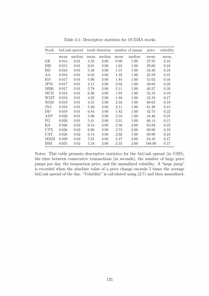
Table 3.1: Descriptive statistics for 19 DJIA stocks
Stock bid/ask spread trade duration number of jumps price volatility
mean median mean median mean median mean meanGE 0.014 0.01 4.58 2.00 0.98 1.00 27.95 0.24DIS 0.015 0.01 6.01 3.00 1.63 1.00 29.60 0.24HD 0.016 0.01 5.48 3.00 1.57 1.00 34.30 0.24AA 0.016 0.01 6.82 3.00 1.32 1.00 25.59 0.31KO 0.017 0.01 5.96 3.00 1.84 1.00 51.62 0.16JPM 0.017 0.01 4.11 2.00 2.02 1.00 38.68 0.28MRK 0.017 0.01 5.78 3.00 2.11 1.00 40.37 0.20MCD 0.018 0.01 6.36 3.00 1.91 1.00 52.18 0.19WMT 0.018 0.01 4.92 2.00 1.88 1.00 52.19 0.17XOM 0.019 0.01 3.55 2.00 2.34 1.00 68.62 0.19JNJ 0.018 0.01 5.40 3.00 2.11 1.00 61.36 0.15DD 0.019 0.01 6.84 3.00 1.82 1.00 42.74 0.22AXP 0.020 0.01 5.90 3.00 2.10 1.00 44.46 0.25PG 0.020 0.01 5.41 3.00 2.31 1.00 66.14 0.15BA 0.026 0.02 6.54 3.00 2.50 2.00 63.88 0.22UTX 0.026 0.02 6.96 3.00 2.73 2.00 69.98 0.19CAT 0.028 0.02 6.14 3.00 2.02 1.00 69.99 0.23MMM 0.029 0.02 7.01 3.00 2.47 2.00 84.10 0.17IBM 0.035 0.02 5.18 3.00 2.35 2.00 108.00 0.17
Notes: This table presents descriptive statistics for the bid/ask spread (in USD),the time between consecutive transactions (in seconds), the number of large pricejumps per day, the transaction price, and the annualized volatility. A “large jump”is recorded when the absolute value of a price change exceeds 5 times the averagebid/ask spread of the day. “Volatility” is calculated using (2.7) and then annualized.
135
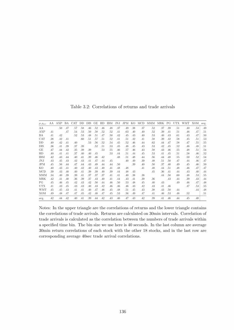
Table 3.2: Correlations of returns and trade arrivals
ρ, ρarr AA AXP BA CAT DD DIS GE HD IBM JNJ JPM KO MCD MMM MRK PG UTX WMT XOM avg.
AA .50 .47 .57 .58 .46 .52 .46 .48 .37 .49 .38 .37 .52 .37 .39 .51 .40 .53 .49AXP .41 .47 .54 .53 .50 .58 .52 .52 .41 .63 .40 .40 .52 .39 .41 .51 .46 .47 .51BA .41 .42 .52 .53 .48 .51 .47 .50 .42 .45 .43 .40 .53 .40 .43 .61 .43 .47 .50CAT .38 .42 .41 .60 .51 .57 .51 .52 .41 .51 .42 .41 .58 .39 .42 .58 .45 .51 .53DD .40 .42 .41 .40 .53 .56 .52 .54 .45 .52 .46 .44 .62 .44 .47 .58 .47 .55 .55DIS .36 .41 .39 .37 .39 .52 .51 .53 .45 .48 .45 .43 .53 .42 .45 .52 .46 .48 .51GE .47 .44 .42 .35 .39 .39 .53 .55 .46 .57 .46 .43 .58 .43 .46 .55 .48 .51 .54HD .40 .41 .41 .37 .40 .40 .45 .53 .44 .51 .44 .45 .53 .41 .45 .51 .58 .46 .52IBM .42 .43 .44 .40 .41 .39 .46 .42 .48 .51 .48 .44 .56 .44 .48 .55 .50 .52 .54JNJ .43 .45 .43 .42 .43 .41 .47 .44 .45 .40 .49 .39 .48 .51 .50 .47 .44 .46 .47JPM .45 .56 .44 .47 .44 .43 .49 .44 .44 .50 .39 .40 .50 .37 .40 .49 .45 .46 .50KO .40 .43 .41 .40 .42 .40 .43 .40 .41 .48 .48 .41 .48 .44 .51 .48 .46 .47 .47MCD .39 .43 .40 .40 .41 .39 .39 .40 .39 .44 .48 .43 .45 .36 .41 .44 .43 .40 .44MMM .34 .40 .39 .39 .41 .37 .37 .37 .41 .41 .40 .38 .38 .44 .50 .60 .48 .53 .55MRK .42 .41 .40 .36 .39 .37 .43 .40 .41 .44 .43 .41 .39 .36 .43 .44 .39 .43 .44PG .45 .46 .45 .42 .43 .42 .50 .44 .46 .50 .53 .48 .45 .40 .43 .49 .46 .47 .48UTX .41 .43 .45 .43 .43 .40 .43 .42 .46 .46 .46 .43 .42 .43 .41 .46 .47 .53 .55WMT .45 .45 .43 .41 .41 .40 .47 .46 .45 .48 .51 .45 .43 .38 .43 .50 .44 .44 .48XOM .49 .48 .47 .47 .45 .42 .48 .47 .45 .53 .56 .49 .47 .41 .46 .53 .48 .52 .51
avg. .42 .44 .42 .40 .41 .39 .44 .42 .43 .46 .47 .43 .42 .39 .41 .46 .44 .45 .48
Notes: In the upper triangle are the correlations of returns and the lower triangle contains
the correlations of trade arrivals. Returns are calculated on 30min intervals. Correlation of
trade arrivals is calculated as the correlation between the numbers of trade arrivals within
a specified time bin. The bin size we use here is 40 seconds. In the last column are average
30min return correlations of each stock with the other 18 stocks, and in the last row are
corresponding average 40sec trade arrival correlations.
136
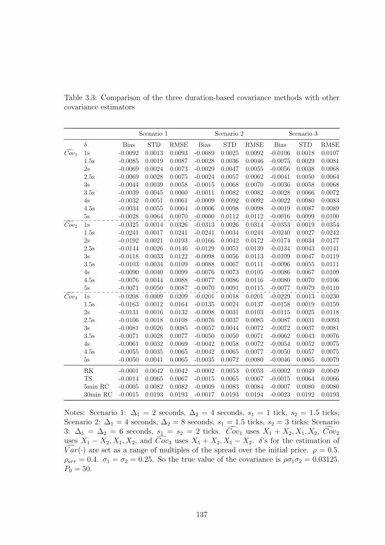
Table 3.3: Comparison of the three duration-based covariance methods with othercovariance estimators
Scenario 1 Scenario 2 Scenario 3
δ Bias STD RMSE Bias STD RMSE Bias STD RMSE
Cov1 1s -0.0092 0.0013 0.0093 -0.0089 0.0025 0.0092 -0.0106 0.0018 0.01071.5s -0.0085 0.0019 0.0087 -0.0028 0.0036 0.0046 -0.0075 0.0029 0.00812s -0.0069 0.0024 0.0073 -0.0029 0.0047 0.0055 -0.0056 0.0038 0.00682.5s -0.0069 0.0028 0.0075 -0.0024 0.0057 0.0062 -0.0041 0.0050 0.00643s -0.0044 0.0039 0.0058 -0.0015 0.0068 0.0070 -0.0036 0.0058 0.00683.5s -0.0039 0.0045 0.0060 -0.0011 0.0082 0.0082 -0.0028 0.0066 0.00724s -0.0032 0.0051 0.0061 -0.0009 0.0092 0.0092 -0.0022 0.0080 0.00834.5s -0.0034 0.0055 0.0064 -0.0006 0.0098 0.0098 -0.0019 0.0087 0.00895s -0.0028 0.0064 0.0070 -0.0000 0.0112 0.0112 -0.0016 0.0099 0.0100
Cov2 1s -0.0325 0.0014 0.0326 -0.0313 0.0026 0.0314 -0.0353 0.0019 0.03541.5s -0.0241 0.0017 0.0241 -0.0241 0.0034 0.0244 -0.0240 0.0027 0.02422s -0.0192 0.0021 0.0193 -0.0166 0.0042 0.0172 -0.0174 0.0034 0.01772.5s -0.0144 0.0026 0.0146 -0.0129 0.0051 0.0139 -0.0134 0.0043 0.01413s -0.0118 0.0033 0.0122 -0.0098 0.0056 0.0113 -0.0109 0.0047 0.01193.5s -0.0103 0.0034 0.0109 -0.0088 0.0067 0.0111 -0.0096 0.0055 0.01114s -0.0090 0.0040 0.0099 -0.0076 0.0073 0.0105 -0.0086 0.0067 0.01094.5s -0.0076 0.0044 0.0088 -0.0077 0.0086 0.0116 -0.0080 0.0070 0.01065s -0.0071 0.0050 0.0087 -0.0070 0.0091 0.0115 -0.0077 0.0079 0.0110
Cov3 1s -0.0208 0.0009 0.0209 -0.0201 0.0018 0.0201 -0.0229 0.0013 0.02301.5s -0.0163 0.0012 0.0164 -0.0135 0.0024 0.0137 -0.0158 0.0019 0.01592s -0.0131 0.0016 0.0132 -0.0098 0.0031 0.0103 -0.0115 0.0025 0.01182.5s -0.0106 0.0018 0.0108 -0.0076 0.0037 0.0085 -0.0087 0.0031 0.00933s -0.0081 0.0026 0.0085 -0.0057 0.0044 0.0072 -0.0072 0.0037 0.00813.5s -0.0071 0.0028 0.0077 -0.0050 0.0050 0.0071 -0.0062 0.0043 0.00764s -0.0061 0.0032 0.0069 -0.0042 0.0058 0.0072 -0.0054 0.0052 0.00754.5s -0.0055 0.0035 0.0065 -0.0042 0.0065 0.0077 -0.0050 0.0057 0.00755s -0.0050 0.0041 0.0065 -0.0035 0.0072 0.0080 -0.0046 0.0065 0.0079
RK -0.0001 0.0042 0.0042 -0.0002 0.0053 0.0053 -0.0002 0.0049 0.0049TS -0.0014 0.0065 0.0067 -0.0015 0.0065 0.0067 -0.0015 0.0064 0.00665min RC -0.0005 0.0082 0.0082 -0.0009 0.0083 0.0084 -0.0007 0.0080 0.008030min RC -0.0015 0.0193 0.0193 -0.0017 0.0193 0.0194 -0.0023 0.0192 0.0193
Notes: Scenario 1: ∆1 = 2 seconds, ∆2 = 4 seconds, s1 = 1 tick, s2 = 1.5 ticks;Scenario 2: ∆1 = 4 seconds, ∆2 = 8 seconds, s1 = 1.5 ticks, s2 = 3 ticks; Scenario3: ∆1 = ∆2 = 6 seconds, s1 = s2 = 2 ticks. Cov1 uses X1 + X2, X1, X2, Cov2uses X1 − X2, X1, X2, and Cov3 uses X1 + X2, X1 − X2. δ’s for the estimation ofV ar(·) are set as a range of multiples of the spread over the initial price. ρ = 0.5.ρarr = 0.4. σ1 = σ2 = 0.25. So the true value of the covariance is ρσ1σ2 = 0.03125.P0 = 50.
137
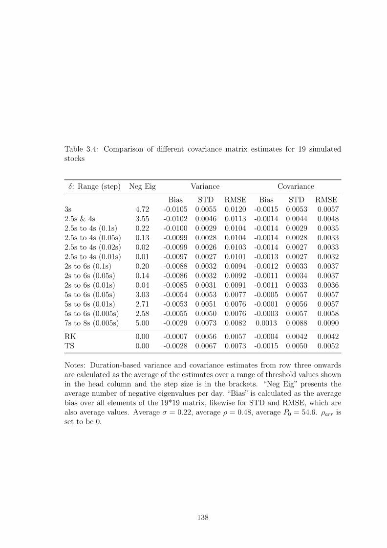
Table 3.4: Comparison of different covariance matrix estimates for 19 simulatedstocks
δ: Range (step) Neg Eig Variance Covariance
Bias STD RMSE Bias STD RMSE3s 4.72 -0.0105 0.0055 0.0120 -0.0015 0.0053 0.00572.5s & 4s 3.55 -0.0102 0.0046 0.0113 -0.0014 0.0044 0.00482.5s to 4s (0.1s) 0.22 -0.0100 0.0029 0.0104 -0.0014 0.0029 0.00352.5s to 4s (0.05s) 0.13 -0.0099 0.0028 0.0104 -0.0014 0.0028 0.00332.5s to 4s (0.02s) 0.02 -0.0099 0.0026 0.0103 -0.0014 0.0027 0.00332.5s to 4s (0.01s) 0.01 -0.0097 0.0027 0.0101 -0.0013 0.0027 0.00322s to 6s (0.1s) 0.20 -0.0088 0.0032 0.0094 -0.0012 0.0033 0.00372s to 6s (0.05s) 0.14 -0.0086 0.0032 0.0092 -0.0011 0.0034 0.00372s to 6s (0.01s) 0.04 -0.0085 0.0031 0.0091 -0.0011 0.0033 0.00365s to 6s (0.05s) 3.03 -0.0054 0.0053 0.0077 -0.0005 0.0057 0.00575s to 6s (0.01s) 2.71 -0.0053 0.0051 0.0076 -0.0001 0.0056 0.00575s to 6s (0.005s) 2.58 -0.0055 0.0050 0.0076 -0.0003 0.0057 0.00587s to 8s (0.005s) 5.00 -0.0029 0.0073 0.0082 0.0013 0.0088 0.0090
RK 0.00 -0.0007 0.0056 0.0057 -0.0004 0.0042 0.0042TS 0.00 -0.0028 0.0067 0.0073 -0.0015 0.0050 0.0052
Notes: Duration-based variance and covariance estimates from row three onwardsare calculated as the average of the estimates over a range of threshold values shownin the head column and the step size is in the brackets. “Neg Eig” presents theaverage number of negative eigenvalues per day. “Bias” is calculated as the averagebias over all elements of the 19*19 matrix, likewise for STD and RMSE, which arealso average values. Average σ = 0.22, average ρ = 0.48, average P0 = 54.6. ρarr isset to be 0.
138
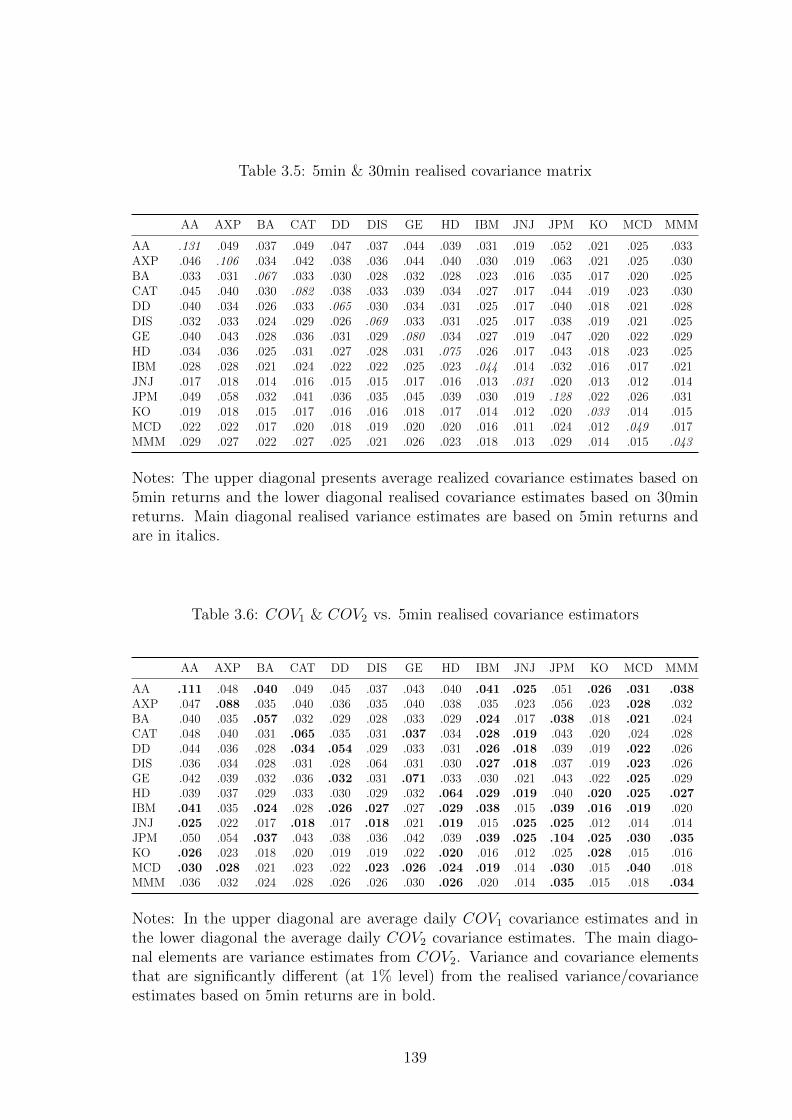
Table 3.5: 5min & 30min realised covariance matrix
AA AXP BA CAT DD DIS GE HD IBM JNJ JPM KO MCD MMM
AA .131 .049 .037 .049 .047 .037 .044 .039 .031 .019 .052 .021 .025 .033AXP .046 .106 .034 .042 .038 .036 .044 .040 .030 .019 .063 .021 .025 .030BA .033 .031 .067 .033 .030 .028 .032 .028 .023 .016 .035 .017 .020 .025CAT .045 .040 .030 .082 .038 .033 .039 .034 .027 .017 .044 .019 .023 .030DD .040 .034 .026 .033 .065 .030 .034 .031 .025 .017 .040 .018 .021 .028DIS .032 .033 .024 .029 .026 .069 .033 .031 .025 .017 .038 .019 .021 .025GE .040 .043 .028 .036 .031 .029 .080 .034 .027 .019 .047 .020 .022 .029HD .034 .036 .025 .031 .027 .028 .031 .075 .026 .017 .043 .018 .023 .025IBM .028 .028 .021 .024 .022 .022 .025 .023 .044 .014 .032 .016 .017 .021JNJ .017 .018 .014 .016 .015 .015 .017 .016 .013 .031 .020 .013 .012 .014JPM .049 .058 .032 .041 .036 .035 .045 .039 .030 .019 .128 .022 .026 .031KO .019 .018 .015 .017 .016 .016 .018 .017 .014 .012 .020 .033 .014 .015MCD .022 .022 .017 .020 .018 .019 .020 .020 .016 .011 .024 .012 .049 .017MMM .029 .027 .022 .027 .025 .021 .026 .023 .018 .013 .029 .014 .015 .043
Notes: The upper diagonal presents average realized covariance estimates based on5min returns and the lower diagonal realised covariance estimates based on 30minreturns. Main diagonal realised variance estimates are based on 5min returns andare in italics.
Table 3.6: COV1 & COV2 vs. 5min realised covariance estimators
AA AXP BA CAT DD DIS GE HD IBM JNJ JPM KO MCD MMM
AA .111 .048 .040 .049 .045 .037 .043 .040 .041 .025 .051 .026 .031 .038AXP .047 .088 .035 .040 .036 .035 .040 .038 .035 .023 .056 .023 .028 .032BA .040 .035 .057 .032 .029 .028 .033 .029 .024 .017 .038 .018 .021 .024CAT .048 .040 .031 .065 .035 .031 .037 .034 .028 .019 .043 .020 .024 .028DD .044 .036 .028 .034 .054 .029 .033 .031 .026 .018 .039 .019 .022 .026DIS .036 .034 .028 .031 .028 .064 .031 .030 .027 .018 .037 .019 .023 .026GE .042 .039 .032 .036 .032 .031 .071 .033 .030 .021 .043 .022 .025 .029HD .039 .037 .029 .033 .030 .029 .032 .064 .029 .019 .040 .020 .025 .027IBM .041 .035 .024 .028 .026 .027 .027 .029 .038 .015 .039 .016 .019 .020JNJ .025 .022 .017 .018 .017 .018 .021 .019 .015 .025 .025 .012 .014 .014JPM .050 .054 .037 .043 .038 .036 .042 .039 .039 .025 .104 .025 .030 .035KO .026 .023 .018 .020 .019 .019 .022 .020 .016 .012 .025 .028 .015 .016MCD .030 .028 .021 .023 .022 .023 .026 .024 .019 .014 .030 .015 .040 .018MMM .036 .032 .024 .028 .026 .026 .030 .026 .020 .014 .035 .015 .018 .034
Notes: In the upper diagonal are average daily COV1 covariance estimates and inthe lower diagonal the average daily COV2 covariance estimates. The main diago-nal elements are variance estimates from COV2. Variance and covariance elementsthat are significantly different (at 1% level) from the realised variance/covarianceestimates based on 5min returns are in bold.
139
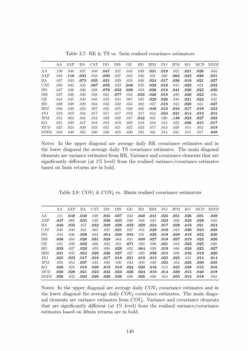
Table 3.7: RK & TS vs. 5min realised covariance estimators
AA AXP BA CAT DD DIS GE HD IBM JNJ JPM KO MCD MMM
AA .139 .048 .037 .049 .047 .037 .043 .039 .031 .019 .052 .021 .026 .034AXP .048 .116 .035 .043 .039 .037 .045 .040 .031 .020 .065 .022 .026 .031BA .037 .033 .073 .035 .031 .029 .034 .030 .024 .017 .036 .019 .021 .027CAT .050 .042 .034 .087 .039 .033 .040 .035 .028 .018 .045 .020 .024 .032DD .047 .038 .030 .038 .070 .032 .036 .033 .026 .018 .041 .020 .022 .030DIS .037 .036 .028 .033 .031 .077 .034 .033 .026 .018 .039 .020 .022 .026GE .044 .045 .033 .040 .035 .034 .087 .035 .029 .020 .048 .021 .023 .032HD .038 .039 .029 .034 .032 .032 .034 .082 .027 .018 .043 .020 .024 .027IBM .030 .029 .023 .027 .025 .025 .028 .026 .049 .016 .034 .017 .019 .023JNJ .019 .019 .016 .017 .017 .017 .019 .017 .014 .034 .021 .014 .013 .015JPM .051 .062 .035 .044 .039 .038 .047 .042 .031 .020 .138 .023 .027 .033KO .021 .020 .017 .019 .018 .019 .020 .018 .016 .013 .022 .036 .015 .017MCD .025 .024 .020 .023 .021 .021 .022 .023 .017 .013 .026 .014 .052 .019MMM .033 .030 .025 .030 .028 .025 .030 .025 .021 .014 .031 .015 .017 .048
Notes: In the upper diagonal are average daily RK covariance estimates and inthe lower diagonal the average daily TS covariance estimates. The main diagonalelements are variance estimates from RK. Variance and covariance elements that aresignificantly different (at 1% level) from the realised variance/covariance estimatesbased on 5min returns are in bold.
Table 3.8: COV1 & COV2 vs. 30min realised covariance estimators
AA AXP BA CAT DD DIS GE HD IBM JNJ JPM KO MCD MMM
AA .111 .048 .040 .049 .045 .037 .043 .040 .041 .025 .051 .026 .031 .038AXP .047 .088 .035 .040 .036 .035 .040 .038 .035 .023 .056 .023 .028 .032BA .040 .035 .057 .032 .029 .028 .033 .029 .024 .017 .038 .018 .021 .024CAT .048 .040 .031 .065 .035 .031 .037 .034 .028 .019 .043 .020 .024 .028DD .044 .036 .028 .034 .054 .029 .033 .031 .026 .018 .039 .019 .022 .026DIS .036 .034 .028 .031 .028 .064 .031 .030 .027 .018 .037 .019 .023 .026GE .042 .039 .032 .036 .032 .031 .071 .033 .030 .021 .043 .022 .025 .029HD .039 .037 .029 .033 .030 .029 .032 .064 .029 .019 .040 .020 .025 .027IBM .041 .035 .024 .028 .026 .027 .027 .029 .038 .015 .039 .016 .019 .020JNJ .025 .022 .017 .018 .017 .018 .021 .019 .015 .025 .025 .012 .014 .014JPM .050 .054 .037 .043 .038 .036 .042 .039 .039 .025 .104 .025 .030 .035KO .026 .023 .018 .020 .019 .019 .022 .020 .016 .012 .025 .028 .015 .016MCD .030 .028 .021 .023 .022 .023 .026 .024 .019 .014 .030 .015 .040 .018MMM .036 .032 .024 .028 .026 .026 .030 .026 .020 .014 .035 .015 .018 .034
Notes: In the upper diagonal are average daily COV1 covariance estimates and inthe lower diagonal the average daily COV2 covariance estimates. The main diago-nal elements are variance estimates from COV2. Variance and covariance elementsthat are significantly different (at 1% level) from the realised variance/covarianceestimates based on 30min returns are in bold.
140
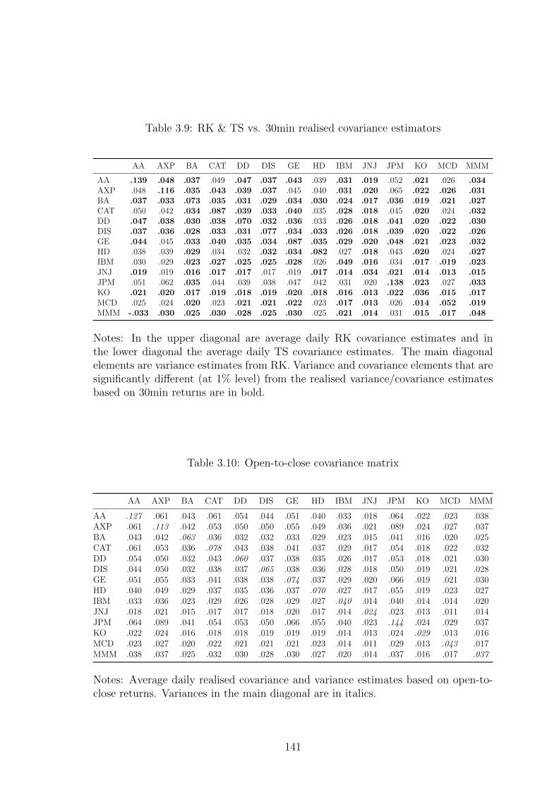
Table 3.9: RK & TS vs. 30min realised covariance estimators
AA AXP BA CAT DD DIS GE HD IBM JNJ JPM KO MCD MMM
AA .139 .048 .037 .049 .047 .037 .043 .039 .031 .019 .052 .021 .026 .034AXP .048 .116 .035 .043 .039 .037 .045 .040 .031 .020 .065 .022 .026 .031BA .037 .033 .073 .035 .031 .029 .034 .030 .024 .017 .036 .019 .021 .027CAT .050 .042 .034 .087 .039 .033 .040 .035 .028 .018 .045 .020 .024 .032DD .047 .038 .030 .038 .070 .032 .036 .033 .026 .018 .041 .020 .022 .030DIS .037 .036 .028 .033 .031 .077 .034 .033 .026 .018 .039 .020 .022 .026GE .044 .045 .033 .040 .035 .034 .087 .035 .029 .020 .048 .021 .023 .032HD .038 .039 .029 .034 .032 .032 .034 .082 .027 .018 .043 .020 .024 .027IBM .030 .029 .023 .027 .025 .025 .028 .026 .049 .016 .034 .017 .019 .023JNJ .019 .019 .016 .017 .017 .017 .019 .017 .014 .034 .021 .014 .013 .015JPM .051 .062 .035 .044 .039 .038 .047 .042 .031 .020 .138 .023 .027 .033KO .021 .020 .017 .019 .018 .019 .020 .018 .016 .013 .022 .036 .015 .017MCD .025 .024 .020 .023 .021 .021 .022 .023 .017 .013 .026 .014 .052 .019MMM -.033 .030 .025 .030 .028 .025 .030 .025 .021 .014 .031 .015 .017 .048
Notes: In the upper diagonal are average daily RK covariance estimates and inthe lower diagonal the average daily TS covariance estimates. The main diagonalelements are variance estimates from RK. Variance and covariance elements that aresignificantly different (at 1% level) from the realised variance/covariance estimatesbased on 30min returns are in bold.
Table 3.10: Open-to-close covariance matrix
AA AXP BA CAT DD DIS GE HD IBM JNJ JPM KO MCD MMM
AA .127 .061 .043 .061 .054 .044 .051 .040 .033 .018 .064 .022 .023 .038AXP .061 .113 .042 .053 .050 .050 .055 .049 .036 .021 .089 .024 .027 .037BA .043 .042 .063 .036 .032 .032 .033 .029 .023 .015 .041 .016 .020 .025CAT .061 .053 .036 .078 .043 .038 .041 .037 .029 .017 .054 .018 .022 .032DD .054 .050 .032 .043 .060 .037 .038 .035 .026 .017 .053 .018 .021 .030DIS .044 .050 .032 .038 .037 .065 .038 .036 .028 .018 .050 .019 .021 .028GE .051 .055 .033 .041 .038 .038 .074 .037 .029 .020 .066 .019 .021 .030HD .040 .049 .029 .037 .035 .036 .037 .070 .027 .017 .055 .019 .023 .027IBM .033 .036 .023 .029 .026 .028 .029 .027 .040 .014 .040 .014 .014 .020JNJ .018 .021 .015 .017 .017 .018 .020 .017 .014 .024 .023 .013 .011 .014JPM .064 .089 .041 .054 .053 .050 .066 .055 .040 .023 .144 .024 .029 .037KO .022 .024 .016 .018 .018 .019 .019 .019 .014 .013 .024 .029 .013 .016MCD .023 .027 .020 .022 .021 .021 .021 .023 .014 .011 .029 .013 .043 .017MMM .038 .037 .025 .032 .030 .028 .030 .027 .020 .014 .037 .016 .017 .037
Notes: Average daily realised covariance and variance estimates based on open-to-close returns. Variances in the main diagonal are in italics.
141
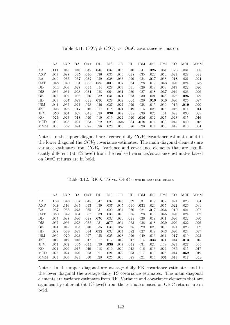
Table 3.11: COV1 & COV2 vs. OtoC covariance estimators
AA AXP BA CAT DD DIS GE HD IBM JNJ JPM KO MCD MMM
AA .111 .048 .040 .049 .045 .037 .043 .040 .041 .025 .051 .026 .031 .038AXP .047 .088 .035 .040 .036 .035 .040 .038 .035 .023 .056 .023 .028 .032BA .040 .035 .057 .032 .029 .028 .033 .029 .024 .017 .038 .018 .021 .024CAT .048 .040 .031 .065 .035 .031 .037 .034 .028 .019 .043 .020 .024 .028DD .044 .036 .028 .034 .054 .029 .033 .031 .026 .018 .039 .019 .022 .026DIS .036 .034 .028 .031 .028 .064 .031 .030 .027 .018 .037 .019 .023 .026GE .042 .039 .032 .036 .032 .031 .071 .033 .030 .021 .043 .022 .025 .029HD .039 .037 .029 .033 .030 .029 .032 .064 .029 .019 .040 .020 .025 .027IBM .041 .035 .024 .028 .026 .027 .027 .029 .038 .015 .039 .016 .019 .020JNJ .025 .022 .017 .018 .017 .018 .021 .019 .015 .025 .025 .012 .014 .014JPM .050 .054 .037 .043 .038 .036 .042 .039 .039 .025 .104 .025 .030 .035KO .026 .023 .018 .020 .019 .019 .022 .020 .016 .012 .025 .028 .015 .016MCD .030 .028 .021 .023 .022 .023 .026 .024 .019 .014 .030 .015 .040 .018MMM .036 .032 .024 .028 .026 .026 .030 .026 .020 .014 .035 .015 .018 .034
Notes: In the upper diagonal are average daily COV1 covariance estimates and inthe lower diagonal the COV2 covariance estimates. The main diagonal elements arevariance estimates from COV2. Variance and covariance elements that are signifi-cantly different (at 1% level) from the realised variance/covariance estimates basedon OtoC returns are in bold.
Table 3.12: RK & TS vs. OtoC covariance estimators
AA AXP BA CAT DD DIS GE HD IBM JNJ JPM KO MCD MMM
AA .139 .048 .037 .049 .047 .037 .043 .039 .031 .019 .052 .021 .026 .034AXP .048 .116 .035 .043 .039 .037 .045 .040 .031 .020 .065 .022 .026 .031BA .037 .033 .073 .035 .031 .029 .034 .030 .024 .017 .036 .019 .021 .027CAT .050 .042 .034 .087 .039 .033 .040 .035 .028 .018 .045 .020 .024 .032DD .047 .038 .030 .038 .070 .032 .036 .033 .026 .018 .041 .020 .022 .030DIS .037 .036 .028 .033 .031 .077 .034 .033 .026 .018 .039 .020 .022 .026GE .044 .045 .033 .040 .035 .034 .087 .035 .029 .020 .048 .021 .023 .032HD .038 .039 .029 .034 .032 .032 .034 .082 .027 .018 .043 .020 .024 .027IBM .030 .029 .023 .027 .025 .025 .028 .026 .049 .016 .034 .017 .019 .023JNJ .019 .019 .016 .017 .017 .017 .019 .017 .014 .034 .021 .014 .013 .015JPM .051 .062 .035 .044 .039 .038 .047 .042 .031 .020 .138 .023 .027 .033KO .021 .020 .017 .019 .018 .019 .020 .018 .016 .013 .022 .036 .015 .017MCD .025 .024 .020 .023 .021 .021 .022 .023 .017 .013 .026 .014 .052 .019MMM .033 .030 .025 .030 .028 .025 .030 .025 .021 .014 .031 .015 .017 .048
Notes: In the upper diagonal are average daily RK covariance estimates and inthe lower diagonal the average daily TS covariance estimates. The main diagonalelements are variance estimates from RK. Variance and covariance elements that aresignificantly different (at 1% level) from the estimates based on OtoC returns are inbold.
142
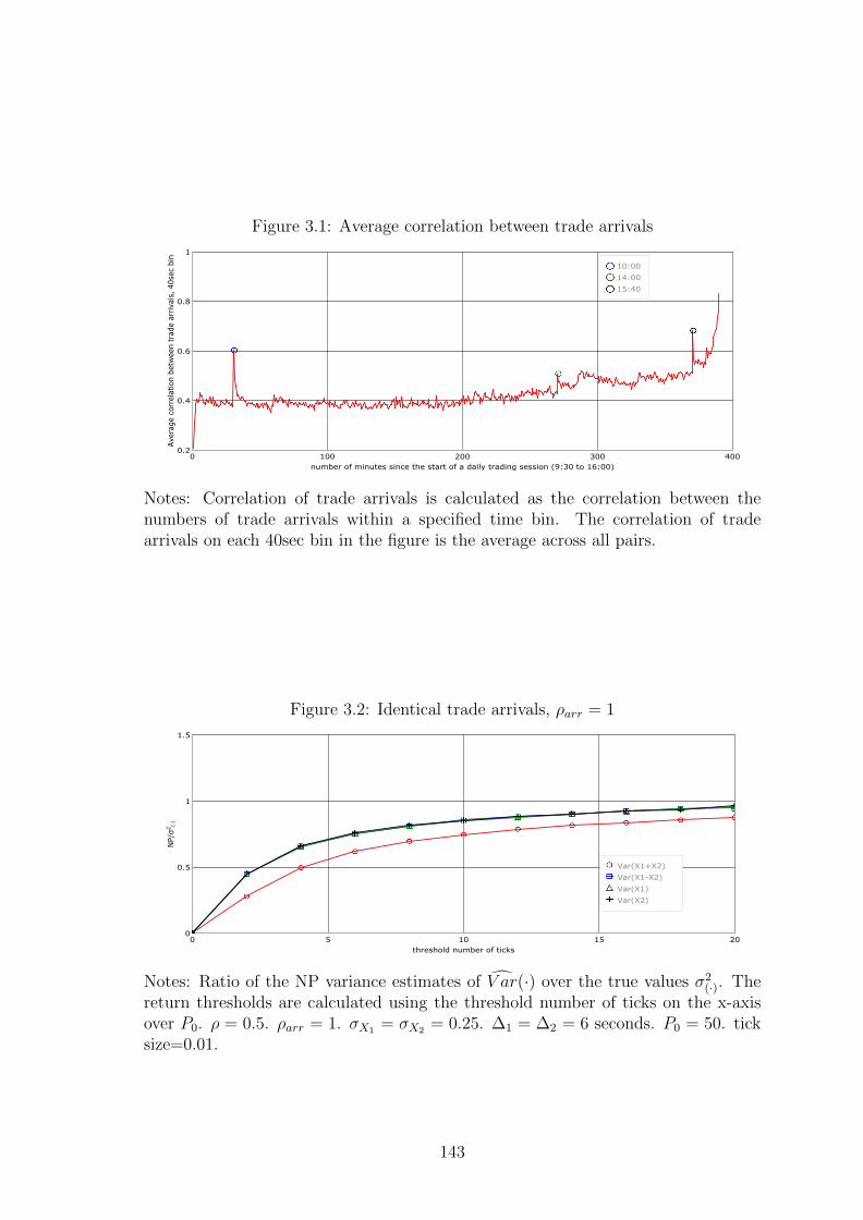
Figure 3.1: Average correlation between trade arrivals
Notes: Correlation of trade arrivals is calculated as the correlation between thenumbers of trade arrivals within a specified time bin. The correlation of tradearrivals on each 40sec bin in the figure is the average across all pairs.
Figure 3.2: Identical trade arrivals, ρarr = 1
Notes: Ratio of the NP variance estimates of V ar(·) over the true values σ2(·). The
return thresholds are calculated using the threshold number of ticks on the x-axisover P0. ρ = 0.5. ρarr = 1. σX1 = σX2 = 0.25. ∆1 = ∆2 = 6 seconds. P0 = 50. ticksize=0.01.
143
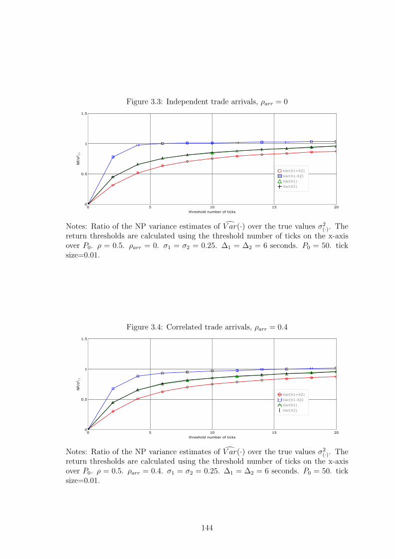
Figure 3.3: Independent trade arrivals, ρarr = 0
Notes: Ratio of the NP variance estimates of V ar(·) over the true values σ2(·). The
return thresholds are calculated using the threshold number of ticks on the x-axisover P0. ρ = 0.5. ρarr = 0. σ1 = σ2 = 0.25. ∆1 = ∆2 = 6 seconds. P0 = 50. ticksize=0.01.
Figure 3.4: Correlated trade arrivals, ρarr = 0.4
Notes: Ratio of the NP variance estimates of V ar(·) over the true values σ2(·). The
return thresholds are calculated using the threshold number of ticks on the x-axisover P0. ρ = 0.5. ρarr = 0.4. σ1 = σ2 = 0.25. ∆1 = ∆2 = 6 seconds. P0 = 50. ticksize=0.01.
144
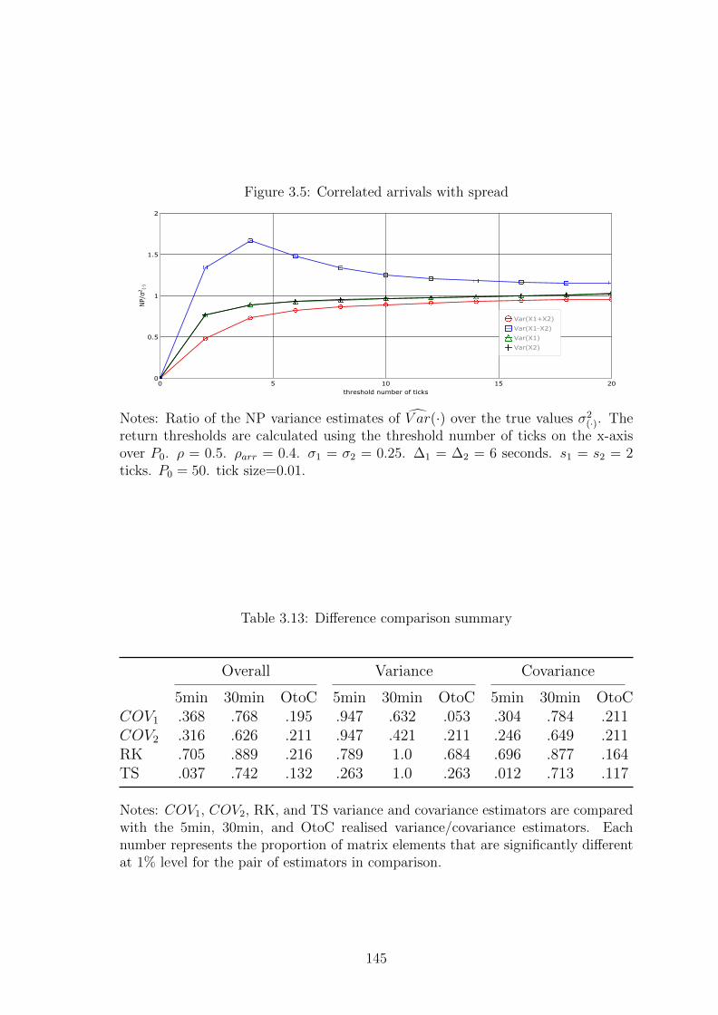
Figure 3.5: Correlated arrivals with spread
Notes: Ratio of the NP variance estimates of V ar(·) over the true values σ2(·). The
return thresholds are calculated using the threshold number of ticks on the x-axisover P0. ρ = 0.5. ρarr = 0.4. σ1 = σ2 = 0.25. ∆1 = ∆2 = 6 seconds. s1 = s2 = 2ticks. P0 = 50. tick size=0.01.
Table 3.13: Difference comparison summary
Overall Variance Covariance
5min 30min OtoC 5min 30min OtoC 5min 30min OtoCCOV1 .368 .768 .195 .947 .632 .053 .304 .784 .211COV2 .316 .626 .211 .947 .421 .211 .246 .649 .211RK .705 .889 .216 .789 1.0 .684 .696 .877 .164TS .037 .742 .132 .263 1.0 .263 .012 .713 .117
Notes: COV1, COV2, RK, and TS variance and covariance estimators are comparedwith the 5min, 30min, and OtoC realised variance/covariance estimators. Eachnumber represents the proportion of matrix elements that are significantly differentat 1% level for the pair of estimators in comparison.
145
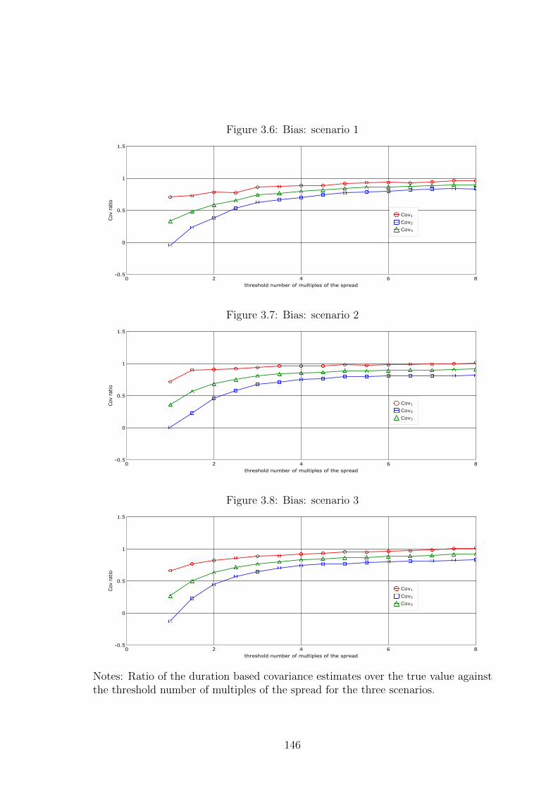
Figure 3.6: Bias: scenario 1
Figure 3.7: Bias: scenario 2
Figure 3.8: Bias: scenario 3
Notes: Ratio of the duration based covariance estimates over the true value againstthe threshold number of multiples of the spread for the three scenarios.
146
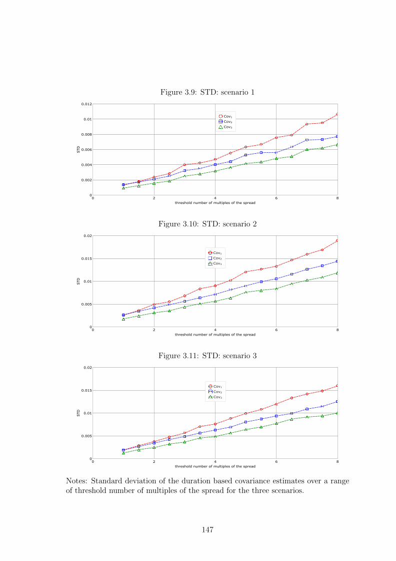
Figure 3.9: STD: scenario 1
Figure 3.10: STD: scenario 2
Figure 3.11: STD: scenario 3
Notes: Standard deviation of the duration based covariance estimates over a rangeof threshold number of multiples of the spread for the three scenarios.
147
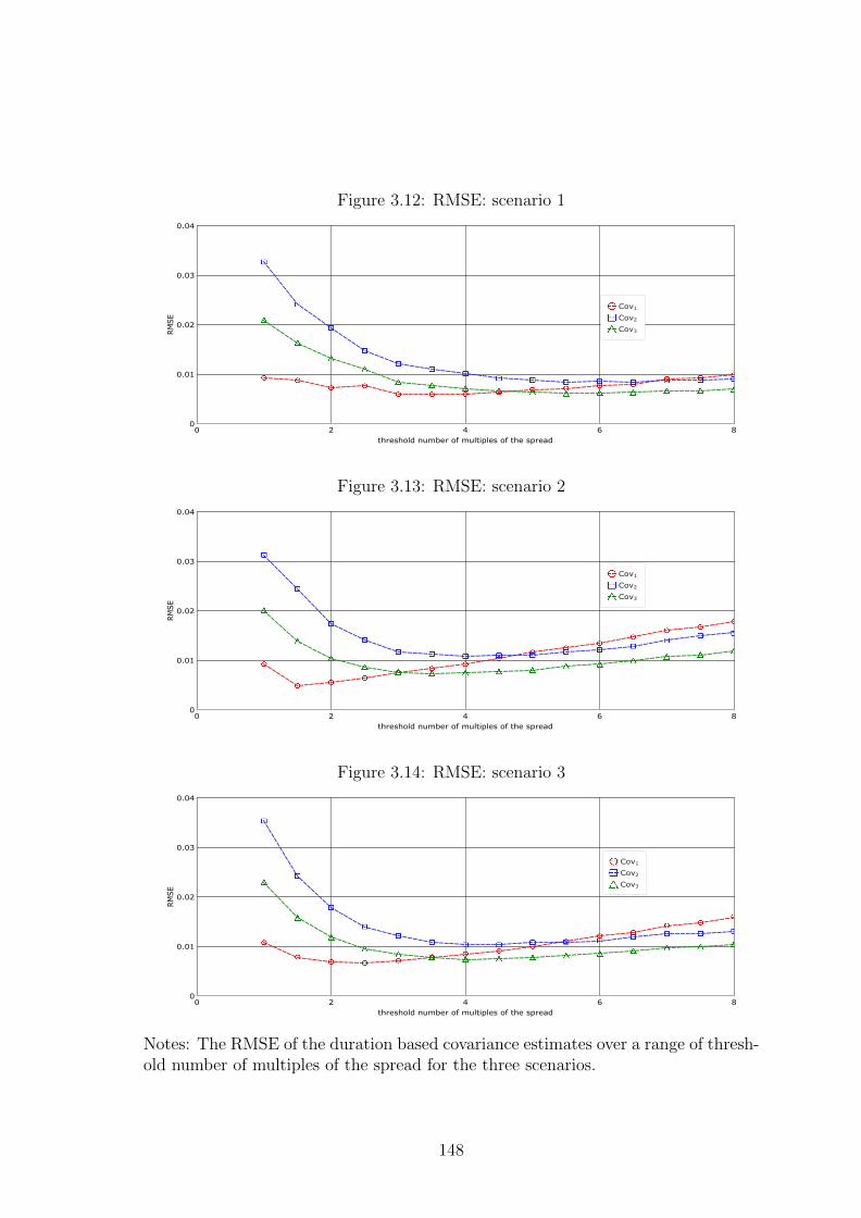
Figure 3.12: RMSE: scenario 1
Figure 3.13: RMSE: scenario 2
Figure 3.14: RMSE: scenario 3
Notes: The RMSE of the duration based covariance estimates over a range of thresh-old number of multiples of the spread for the three scenarios.
148
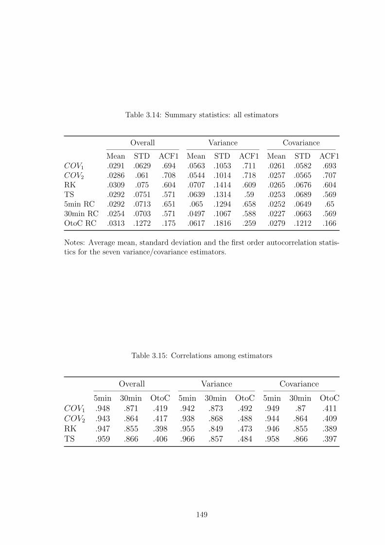
Table 3.14: Summary statistics: all estimators
Overall Variance Covariance
Mean STD ACF1 Mean STD ACF1 Mean STD ACF1COV1 .0291 .0629 .694 .0563 .1053 .711 .0261 .0582 .693COV2 .0286 .061 .708 .0544 .1014 .718 .0257 .0565 .707RK .0309 .075 .604 .0707 .1414 .609 .0265 .0676 .604TS .0292 .0751 .571 .0639 .1314 .59 .0253 .0689 .5695min RC .0292 .0713 .651 .065 .1294 .658 .0252 .0649 .6530min RC .0254 .0703 .571 .0497 .1067 .588 .0227 .0663 .569OtoC RC .0313 .1272 .175 .0617 .1816 .259 .0279 .1212 .166
Notes: Average mean, standard deviation and the first order autocorrelation statis-tics for the seven variance/covariance estimators.
Table 3.15: Correlations among estimators
Overall Variance Covariance
5min 30min OtoC 5min 30min OtoC 5min 30min OtoCCOV1 .948 .871 .419 .942 .873 .492 .949 .87 .411COV2 .943 .864 .417 .938 .868 .488 .944 .864 .409RK .947 .855 .398 .955 .849 .473 .946 .855 .389TS .959 .866 .406 .966 .857 .484 .958 .866 .397
149
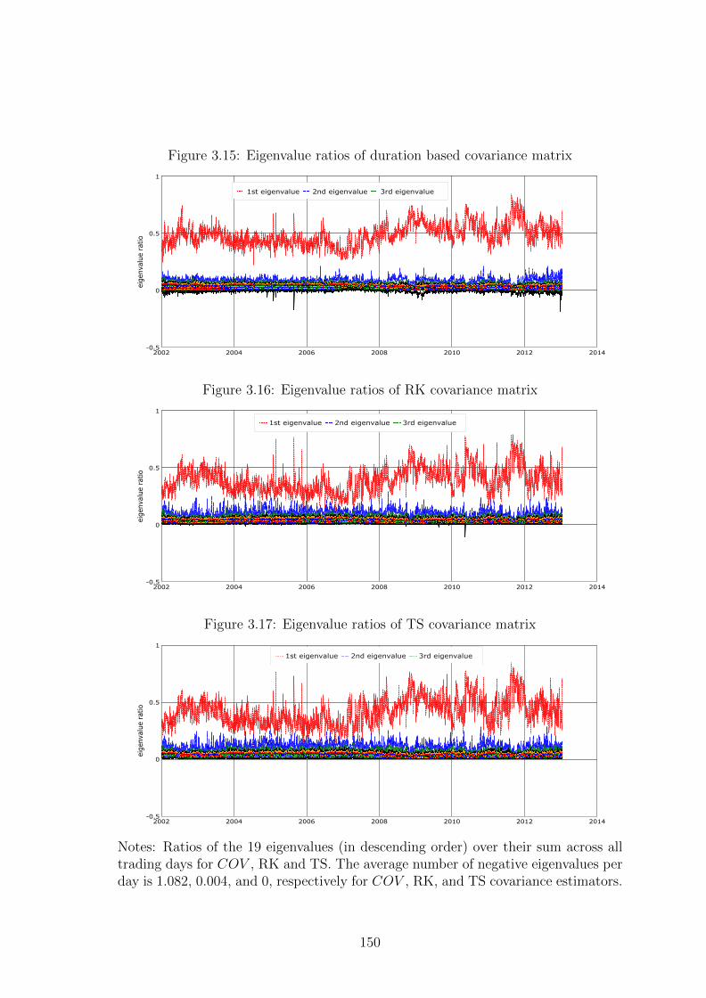
Figure 3.15: Eigenvalue ratios of duration based covariance matrix
Figure 3.16: Eigenvalue ratios of RK covariance matrix
Figure 3.17: Eigenvalue ratios of TS covariance matrix
Notes: Ratios of the 19 eigenvalues (in descending order) over their sum across alltrading days for COV , RK and TS. The average number of negative eigenvalues perday is 1.082, 0.004, and 0, respectively for COV , RK, and TS covariance estimators.
150
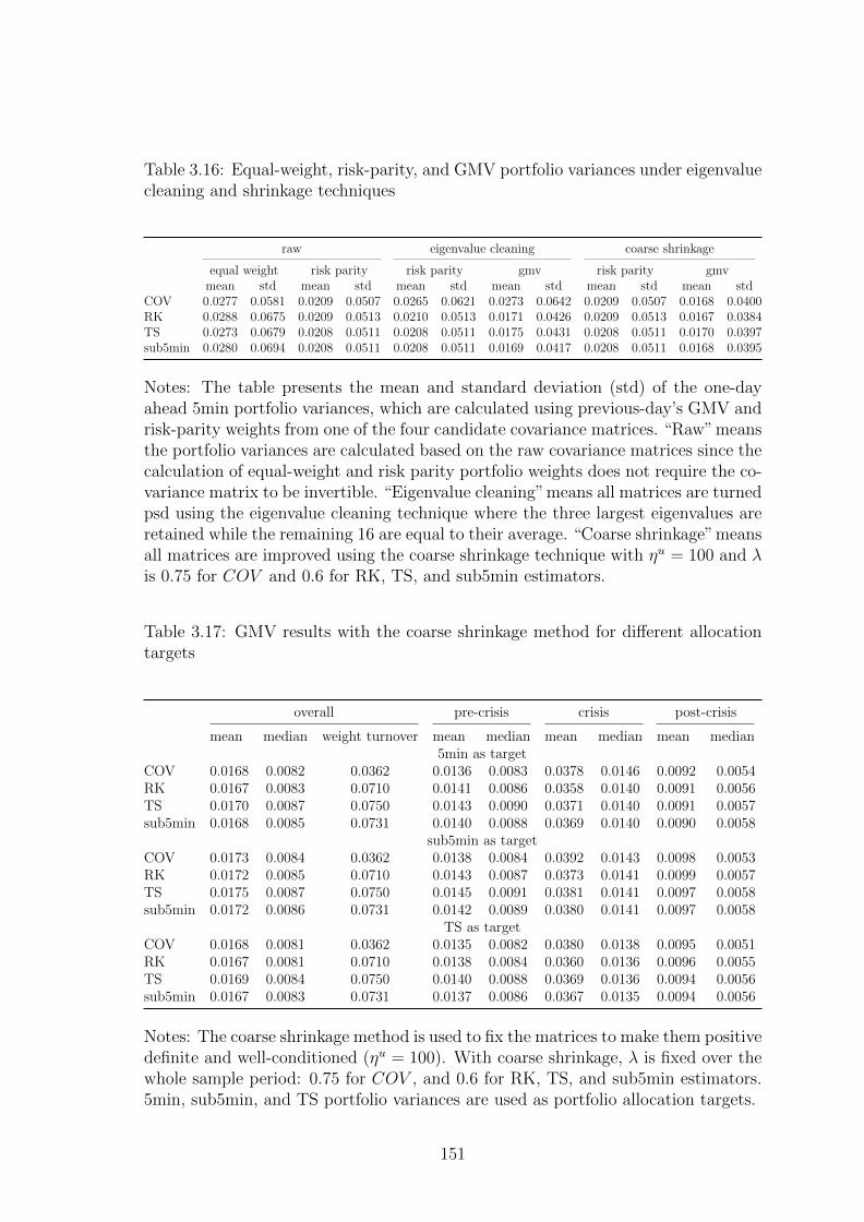
Table 3.16: Equal-weight, risk-parity, and GMV portfolio variances under eigenvaluecleaning and shrinkage techniques
raw eigenvalue cleaning coarse shrinkage
equal weight risk parity risk parity gmv risk parity gmvmean std mean std mean std mean std mean std mean std
COV 0.0277 0.0581 0.0209 0.0507 0.0265 0.0621 0.0273 0.0642 0.0209 0.0507 0.0168 0.0400RK 0.0288 0.0675 0.0209 0.0513 0.0210 0.0513 0.0171 0.0426 0.0209 0.0513 0.0167 0.0384TS 0.0273 0.0679 0.0208 0.0511 0.0208 0.0511 0.0175 0.0431 0.0208 0.0511 0.0170 0.0397sub5min 0.0280 0.0694 0.0208 0.0511 0.0208 0.0511 0.0169 0.0417 0.0208 0.0511 0.0168 0.0395
Notes: The table presents the mean and standard deviation (std) of the one-dayahead 5min portfolio variances, which are calculated using previous-day’s GMV andrisk-parity weights from one of the four candidate covariance matrices. “Raw”meansthe portfolio variances are calculated based on the raw covariance matrices since thecalculation of equal-weight and risk parity portfolio weights does not require the co-variance matrix to be invertible. “Eigenvalue cleaning”means all matrices are turnedpsd using the eigenvalue cleaning technique where the three largest eigenvalues areretained while the remaining 16 are equal to their average. “Coarse shrinkage”meansall matrices are improved using the coarse shrinkage technique with ηu = 100 and λis 0.75 for COV and 0.6 for RK, TS, and sub5min estimators.
Table 3.17: GMV results with the coarse shrinkage method for different allocationtargets
overall pre-crisis crisis post-crisis
mean median weight turnover mean median mean median mean median5min as target
COV 0.0168 0.0082 0.0362 0.0136 0.0083 0.0378 0.0146 0.0092 0.0054RK 0.0167 0.0083 0.0710 0.0141 0.0086 0.0358 0.0140 0.0091 0.0056TS 0.0170 0.0087 0.0750 0.0143 0.0090 0.0371 0.0140 0.0091 0.0057sub5min 0.0168 0.0085 0.0731 0.0140 0.0088 0.0369 0.0140 0.0090 0.0058
sub5min as targetCOV 0.0173 0.0084 0.0362 0.0138 0.0084 0.0392 0.0143 0.0098 0.0053RK 0.0172 0.0085 0.0710 0.0143 0.0087 0.0373 0.0141 0.0099 0.0057TS 0.0175 0.0087 0.0750 0.0145 0.0091 0.0381 0.0141 0.0097 0.0058sub5min 0.0172 0.0086 0.0731 0.0142 0.0089 0.0380 0.0141 0.0097 0.0058
TS as targetCOV 0.0168 0.0081 0.0362 0.0135 0.0082 0.0380 0.0138 0.0095 0.0051RK 0.0167 0.0081 0.0710 0.0138 0.0084 0.0360 0.0136 0.0096 0.0055TS 0.0169 0.0084 0.0750 0.0140 0.0088 0.0369 0.0136 0.0094 0.0056sub5min 0.0167 0.0083 0.0731 0.0137 0.0086 0.0367 0.0135 0.0094 0.0056
Notes: The coarse shrinkage method is used to fix the matrices to make them positivedefinite and well-conditioned (ηu = 100). With coarse shrinkage, λ is fixed over thewhole sample period: 0.75 for COV , and 0.6 for RK, TS, and sub5min estimators.5min, sub5min, and TS portfolio variances are used as portfolio allocation targets.
151
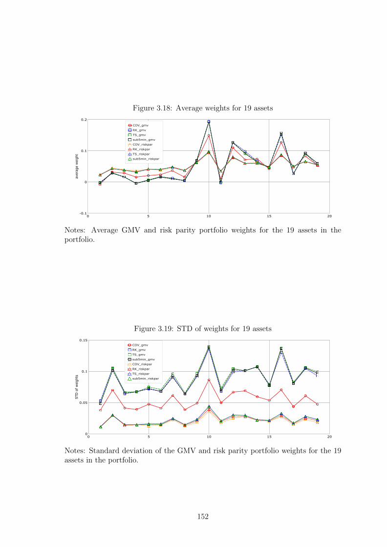
Figure 3.18: Average weights for 19 assets
Notes: Average GMV and risk parity portfolio weights for the 19 assets in theportfolio.
Figure 3.19: STD of weights for 19 assets
Notes: Standard deviation of the GMV and risk parity portfolio weights for the 19assets in the portfolio.
152
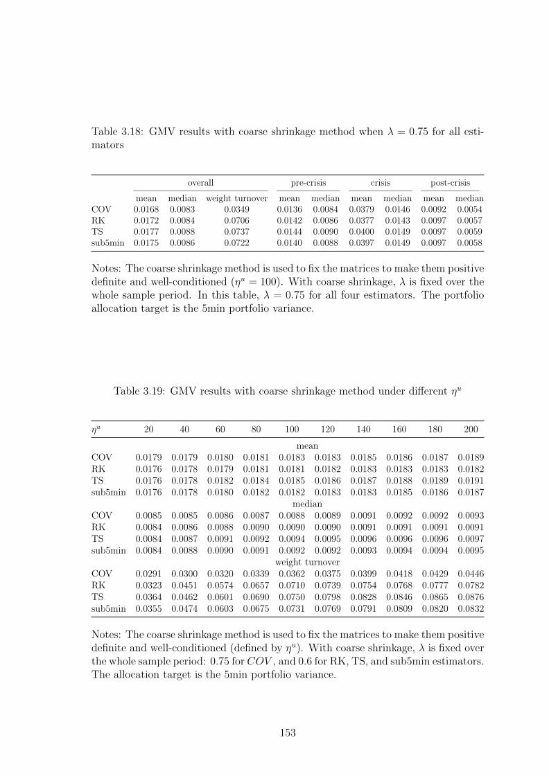
Table 3.18: GMV results with coarse shrinkage method when λ = 0.75 for all esti-mators
overall pre-crisis crisis post-crisis
mean median weight turnover mean median mean median mean medianCOV 0.0168 0.0083 0.0349 0.0136 0.0084 0.0379 0.0146 0.0092 0.0054RK 0.0172 0.0084 0.0706 0.0142 0.0086 0.0377 0.0143 0.0097 0.0057TS 0.0177 0.0088 0.0737 0.0144 0.0090 0.0400 0.0149 0.0097 0.0059sub5min 0.0175 0.0086 0.0722 0.0140 0.0088 0.0397 0.0149 0.0097 0.0058
Notes: The coarse shrinkage method is used to fix the matrices to make them positivedefinite and well-conditioned (ηu = 100). With coarse shrinkage, λ is fixed over thewhole sample period. In this table, λ = 0.75 for all four estimators. The portfolioallocation target is the 5min portfolio variance.
Table 3.19: GMV results with coarse shrinkage method under different ηu
ηu 20 40 60 80 100 120 140 160 180 200
meanCOV 0.0179 0.0179 0.0180 0.0181 0.0183 0.0183 0.0185 0.0186 0.0187 0.0189RK 0.0176 0.0178 0.0179 0.0181 0.0181 0.0182 0.0183 0.0183 0.0183 0.0182TS 0.0176 0.0178 0.0182 0.0184 0.0185 0.0186 0.0187 0.0188 0.0189 0.0191sub5min 0.0176 0.0178 0.0180 0.0182 0.0182 0.0183 0.0183 0.0185 0.0186 0.0187
medianCOV 0.0085 0.0085 0.0086 0.0087 0.0088 0.0089 0.0091 0.0092 0.0092 0.0093RK 0.0084 0.0086 0.0088 0.0090 0.0090 0.0090 0.0091 0.0091 0.0091 0.0091TS 0.0084 0.0087 0.0091 0.0092 0.0094 0.0095 0.0096 0.0096 0.0096 0.0097sub5min 0.0084 0.0088 0.0090 0.0091 0.0092 0.0092 0.0093 0.0094 0.0094 0.0095
weight turnoverCOV 0.0291 0.0300 0.0320 0.0339 0.0362 0.0375 0.0399 0.0418 0.0429 0.0446RK 0.0323 0.0451 0.0574 0.0657 0.0710 0.0739 0.0754 0.0768 0.0777 0.0782TS 0.0364 0.0462 0.0601 0.0690 0.0750 0.0798 0.0828 0.0846 0.0865 0.0876sub5min 0.0355 0.0474 0.0603 0.0675 0.0731 0.0769 0.0791 0.0809 0.0820 0.0832
Notes: The coarse shrinkage method is used to fix the matrices to make them positivedefinite and well-conditioned (defined by ηu). With coarse shrinkage, λ is fixed overthe whole sample period: 0.75 for COV , and 0.6 for RK, TS, and sub5min estimators.The allocation target is the 5min portfolio variance.
153
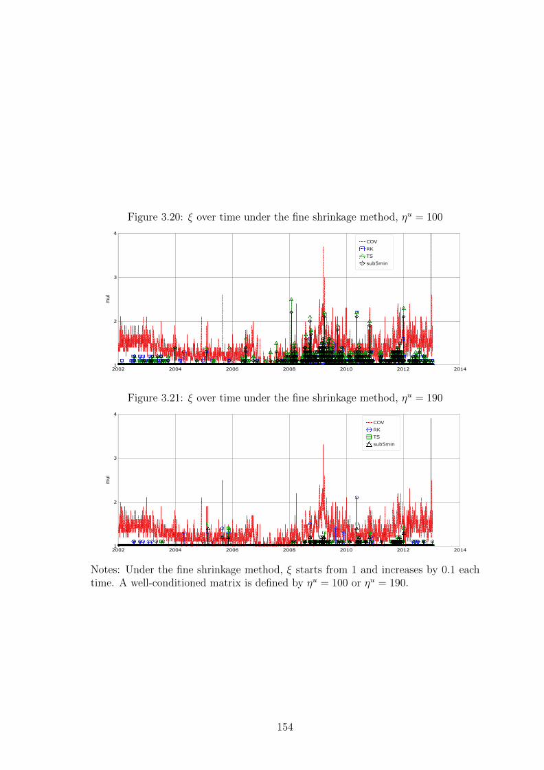
Figure 3.20: ξ over time under the fine shrinkage method, ηu = 100
Figure 3.21: ξ over time under the fine shrinkage method, ηu = 190
Notes: Under the fine shrinkage method, ξ starts from 1 and increases by 0.1 eachtime. A well-conditioned matrix is defined by ηu = 100 or ηu = 190.
154
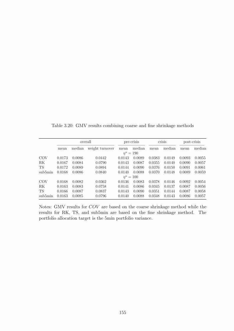
Table 3.20: GMV results combining coarse and fine shrinkage methods
overall pre-crisis crisis post-crisis
mean median weight turnover mean median mean median mean medianηu = 190
COV 0.0173 0.0086 0.0442 0.0143 0.0089 0.0383 0.0149 0.0093 0.0055RK 0.0167 0.0084 0.0790 0.0143 0.0087 0.0355 0.0140 0.0090 0.0057TS 0.0172 0.0089 0.0894 0.0144 0.0090 0.0376 0.0150 0.0091 0.0061sub5min 0.0168 0.0086 0.0840 0.0140 0.0088 0.0370 0.0148 0.0089 0.0059
ηu = 100COV 0.0168 0.0082 0.0362 0.0136 0.0083 0.0378 0.0146 0.0092 0.0054RK 0.0163 0.0083 0.0758 0.0141 0.0086 0.0345 0.0137 0.0087 0.0056TS 0.0166 0.0087 0.0837 0.0143 0.0090 0.0351 0.0144 0.0087 0.0058sub5min 0.0163 0.0085 0.0796 0.0140 0.0088 0.0348 0.0143 0.0086 0.0057
Notes: GMV results for COV are based on the coarse shrinkage method while theresults for RK, TS, and sub5min are based on the fine shrinkage method. Theportfolio allocation target is the 5min portfolio variance.
155
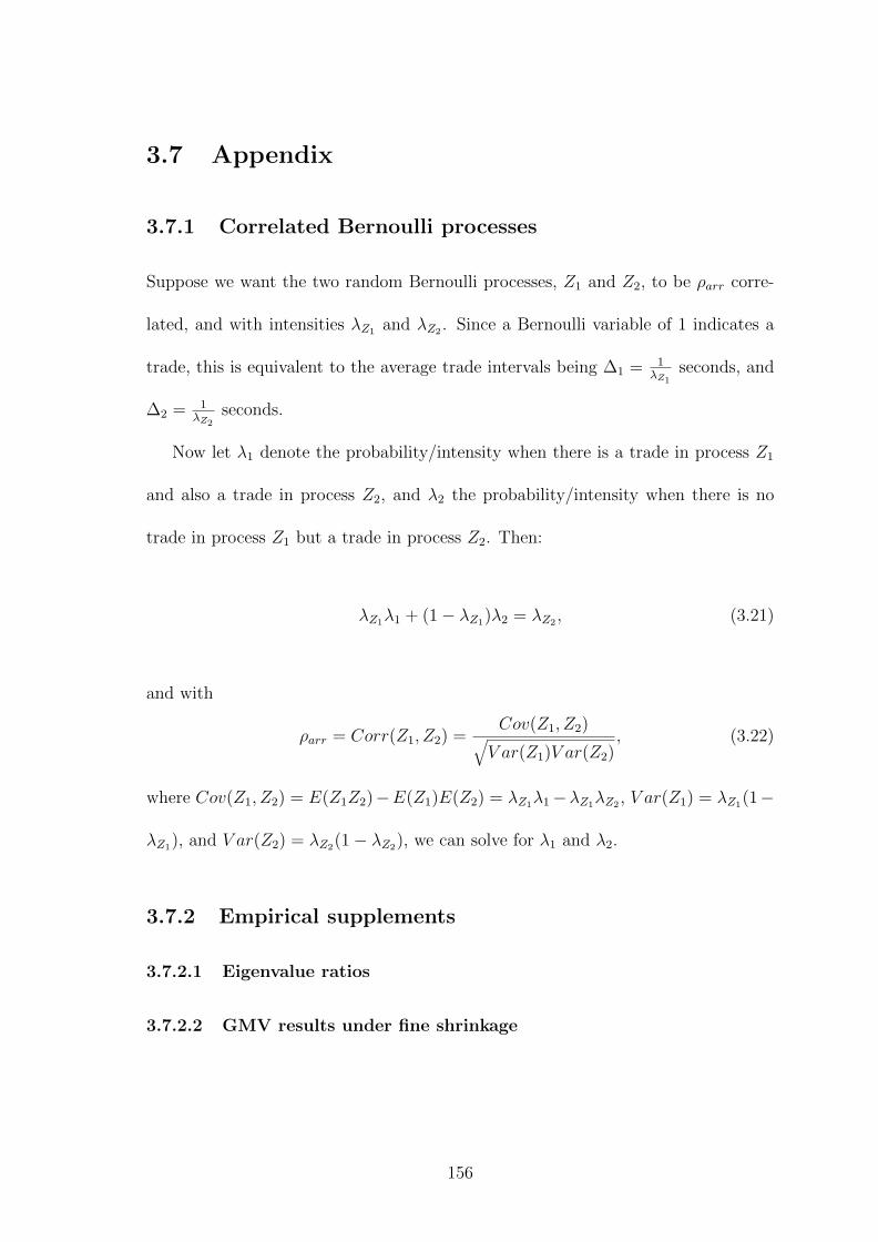
3.7 Appendix
3.7.1 Correlated Bernoulli processes
Suppose we want the two random Bernoulli processes, Z1 and Z2, to be ρarr corre-
lated, and with intensities λZ1 and λZ2 . Since a Bernoulli variable of 1 indicates a
trade, this is equivalent to the average trade intervals being ∆1 = 1λZ1
seconds, and
∆2 = 1λZ2
seconds.
Now let λ1 denote the probability/intensity when there is a trade in process Z1
and also a trade in process Z2, and λ2 the probability/intensity when there is no
trade in process Z1 but a trade in process Z2. Then:
λZ1λ1 + (1− λZ1)λ2 = λZ2 , (3.21)
and with
ρarr = Corr(Z1, Z2) = Cov(Z1, Z2)√V ar(Z1)V ar(Z2)
, (3.22)
where Cov(Z1, Z2) = E(Z1Z2)−E(Z1)E(Z2) = λZ1λ1−λZ1λZ2 , V ar(Z1) = λZ1(1−
λZ1), and V ar(Z2) = λZ2(1− λZ2), we can solve for λ1 and λ2.
3.7.2 Empirical supplements
3.7.2.1 Eigenvalue ratios
3.7.2.2 GMV results under fine shrinkage
156
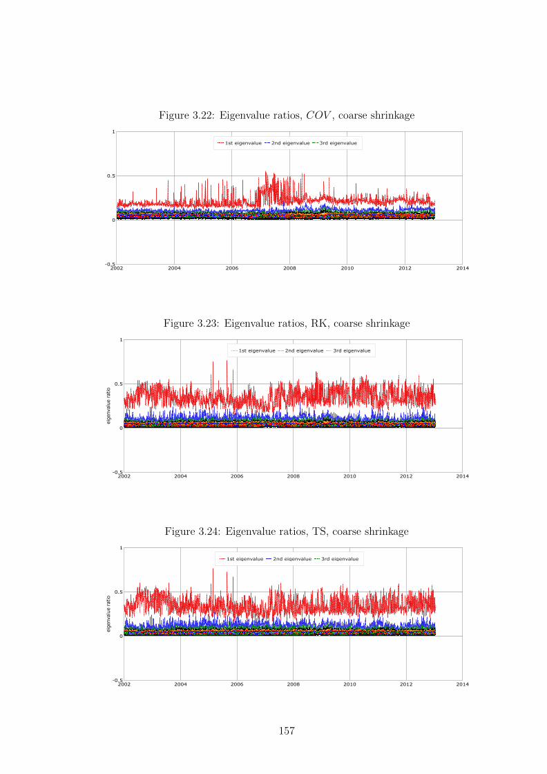
Figure 3.22: Eigenvalue ratios, COV , coarse shrinkage
Figure 3.23: Eigenvalue ratios, RK, coarse shrinkage
Figure 3.24: Eigenvalue ratios, TS, coarse shrinkage
157
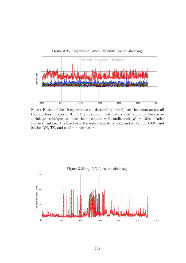
Figure 3.25: Eigenvalue ratios, sub5min, coarse shrinkage
Notes: Ratios of the 19 eigenvalues (in descending order) over their sum across alltrading days for COV , RK, TS and sub5min estimators after applying the coarseshrinkage technique to make them psd and well-conditioned (ηu = 100). Undercoarse shrinkage, λ is fixed over the entire sample period, and is 0.75 for COV and0.6 for RK, TS, and sub5min estimators.
Figure 3.26: η, COV , coarse shrinkage
158
Figure 3.27: η, RK, coarse shrinkage
Figure 3.28: η, TS, coarse shrinkage
Figure 3.29: η, sub5min, coarse shrinkage
Notes: The ratio of largest/smallest eigenvalues (η) after applying the coarseshrinkage technique to make the resulting matrices psd and well conditioned:ηu = 100. Under coarse shrinkage, λ is fixed over the entire sample period, and is0.75 for COV and 0.6 for RK, TS, and sub5min estimators.
159
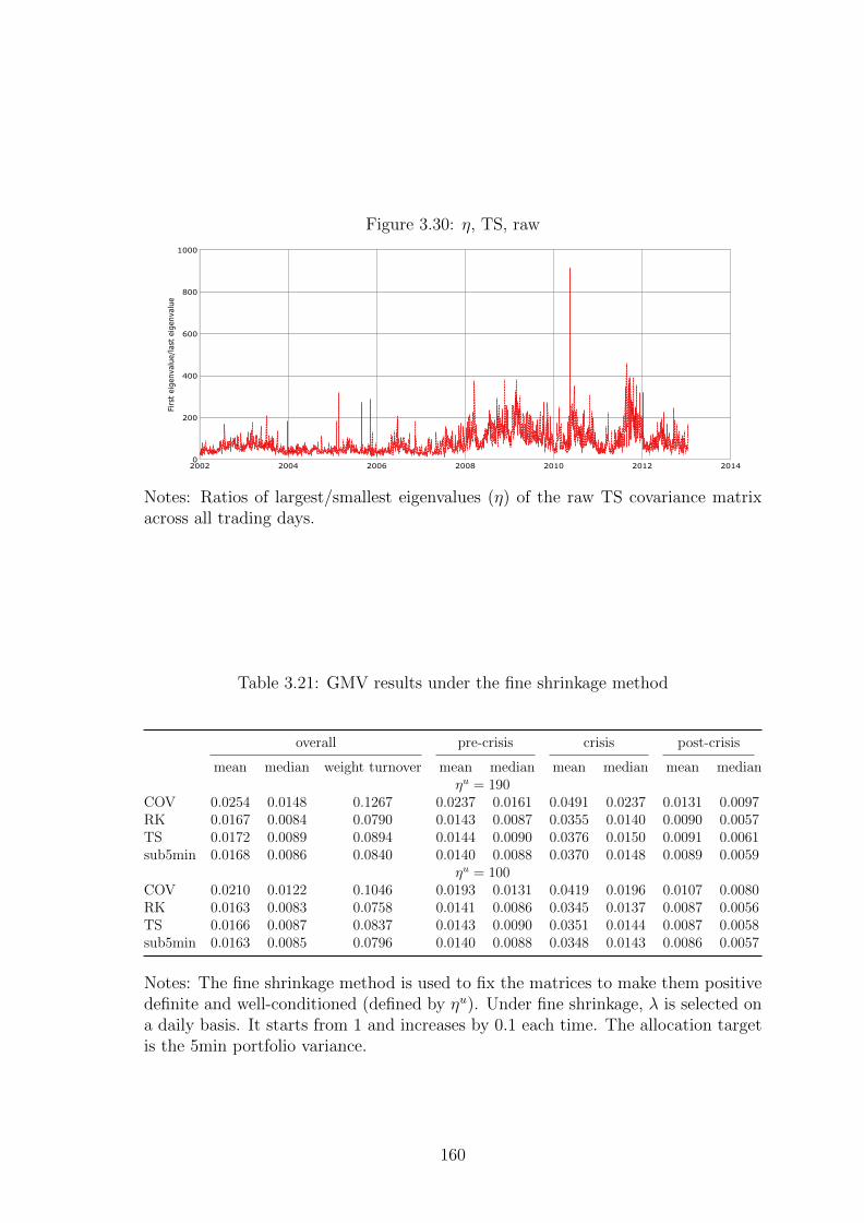
Figure 3.30: η, TS, raw
Notes: Ratios of largest/smallest eigenvalues (η) of the raw TS covariance matrixacross all trading days.
Table 3.21: GMV results under the fine shrinkage method
overall pre-crisis crisis post-crisis
mean median weight turnover mean median mean median mean medianηu = 190
COV 0.0254 0.0148 0.1267 0.0237 0.0161 0.0491 0.0237 0.0131 0.0097RK 0.0167 0.0084 0.0790 0.0143 0.0087 0.0355 0.0140 0.0090 0.0057TS 0.0172 0.0089 0.0894 0.0144 0.0090 0.0376 0.0150 0.0091 0.0061sub5min 0.0168 0.0086 0.0840 0.0140 0.0088 0.0370 0.0148 0.0089 0.0059
ηu = 100COV 0.0210 0.0122 0.1046 0.0193 0.0131 0.0419 0.0196 0.0107 0.0080RK 0.0163 0.0083 0.0758 0.0141 0.0086 0.0345 0.0137 0.0087 0.0056TS 0.0166 0.0087 0.0837 0.0143 0.0090 0.0351 0.0144 0.0087 0.0058sub5min 0.0163 0.0085 0.0796 0.0140 0.0088 0.0348 0.0143 0.0086 0.0057
Notes: The fine shrinkage method is used to fix the matrices to make them positivedefinite and well-conditioned (defined by ηu). Under fine shrinkage, λ is selected ona daily basis. It starts from 1 and increases by 0.1 each time. The allocation targetis the 5min portfolio variance.
160
Concluding remarks
This thesis is consisted of a literature review and two papers, investigating respec-
tively high-frequency variance and covariance estimation using price durations. The
price duration approach to study high-frequency data has received very little atten-
tion in the literature so far. The two papers aim to fill this gap.
The duration approach counts the number of price durations, defined as the time
taken for the absolute cumulative price change to exceed a selected threshold value.
Under this approach, grids are imposed along the price dimension instead of the time
dimension. The tuning parameter under the duration based approach is the optimal
threshold value, which is the point where the impact of MMS noise and price jumps
is mostly mitigated and the RMSE is the smallest. Through simulation evidence
and empirical analysis, we recommend an appropriate choice of threshold value to
be three times the average bid/ask spread. In an volatility forecasting application,
both the parametric and nonparametric price duration volatility estimators are found
to outperform competing RV class and option-implied class of estimators.
We construct the duration based variance-covariance matrix on a pairwise basis.
To decrease the number of negative eigenvalues, we devise an averaging estimator
by taking an average over a wide range of duration-based covariance estimators. We
161
find through simulation evidence that this averaging estimator not only decreases
the number of negative eigenvalues but also improves efficiency. As an empirical ap-
plication, an out-of-sample GMV portfolio allocation problem is studied. The price
duration matrix estimator is found to generate comparably low portfolio variance
with much lower portfolio turnover rates.
In terms of bias and efficiency, comparing to other estimators, the duration based
variance estimates show smaller deviation but larger bias, while the covariance es-
timates using price durations exhibit smaller variation without producing a larger
bias.
For future research, we could think of a way to eliminate the bias of the duration
based variance estimates. The duration based variance and covariance estimators
can also be applied on other asset classes, for example the foreign exchange mar-
kets. We can also devise jump detection methods using price durations, through
the instantaneous volatility estimator produced by the parametric duration based
variance estimator. Research on data with even richer information can include limit
order book dynamics, made possible by the recently available limit order book data.
162
Bibliography
Ait-Sahalia, Yacine, “Estimating continuous-time models with discretely sampled
data,” Econometric Society Monographs, 2007, 43, 261.
and Loriano Mancini, “Out of Sample Forecasts of Quadratic Variation,”
Journal of Econometrics, 2008, 147, 17–33.
, Jianqing Fan, and Dacheng Xiu, “High-Frequency Covariance Estimates
With Noisy and Asynchronous Financial Data,” Journal of the American Sta-
tistical Association, 2010, 105, 1504–1517.
, Per Mykland, and Lan Zhang, “How Often to Sample a Continuous-Time
Process in the Presence of Market Microstructure Noise,” Review of Financial
Studies, 2005, 18, 351–416.
, , and , “Ultra High Frequency Volatility Estimation with Dependent
Microstructure Noise,” Journal of Econometrics, 2011, 160, 160–175.
Alizadeh, S., Michael Brandt, and Francis Diebold, “Range-based estimation
of stochastic volatility models,” Journal of Finance, 2002, 57, 1047–1091.
163
Andersen, Torben, “Return Volatility and Trading Volume: An Information Flow
Interpretation of Stochastic Volatility,” Journal of Finance, 1996, 51, 169–204.
and Tim Bollerslev, “Heterogeneous Information Arrivals and Return
Volatility Dynamics: Uncovering the Long-Run in High Frequency Returns,”
Journal of Finance, 1997, 52, 975–1005.
, Dobrislav Dobrev, and Ernst Schaumburg, “Duration-Based Volatility
Estimation,” 2008. Working Paper, Northwestern University.
, Tim Bollerslev, and Dobrislav Dobrev, “No-arbitrage Semi-martingale
Restrictions for Continuous-time Volatility Models Subject to Leverage Effects,
Jumps and i.i.d. Noise: Theory and Testable Distributional Implications,” Jour-
nal of Econometrics, 2007, 138 (1), 125 – 180.
, , and Francis Diebold, “Parametric and Nonparametric Volatility Mea-
surement,” 2002. Working Paper, National Bureau of Economic Research.
, , and Nour Meddahi, “Realized Volatility Forecasting and Market
Microstructure Noise,” Journal of Econometrics, 2011, 160, 220–234.
, , Francis Diebold, and Heiko Ebens, “The Distribution of Realized
Stock Return Volatility,” Journal of Financial Economics, 2001, 61, 43–76.
, , , and Paul Labys, “Great Realizations,” Risk, 2000, 13, 105–108.
Areal, Nelson and Stephen J. Taylor, “The Realized Volatility of FTSE-100
Futures Prices,” Journal of Futures Markets, 2002, 22, 627–648.
164
Baillie, Richard, Tim Bollerslev, and Hans Mikkelsen, “Fractionally Inte-
grated Generalized Autoregressive Conditional Heteroskedasticity,” Journal of
Econometrics, 1996, 74, 3–30.
Bali, Turan and David Weinbaum, “A Conditional Extreme Value Volatility
Estimator Based on High-Frequency Returns,” Journal of Economic Dynamics
& Control, 2007, 31, 361–397.
Bandi, Federico and Jeffrey Russell, “Separating Microstructure Noise from
Volatility,” Journal of Financial Economics, 2006, 79, 655–692.
and , “Microstructure Noise, Realized Variance, and Optimal Sampling,”
The Review of Economic Studies, 2008, 75, 339–369.
, , and Chen Yang, “Realized Volatility Forecasting in the Presence
of Time-Varying Noise,” Journal of Business & Economic Statistics, 2013,
pp. 331–345.
Barndorff-Nielsen, Ole and Neil Shephard, “Non-Gaussian Ornstein-
Uhlenbeck based Models and Some of Their Uses in Financial Economics,”
Journal of the Royal Statistical Society, 2001, 63 (2), 167–241.
and , “Econometric Analysis of Realized Volatility and Its Use in Esti-
mating Stochastic Volatility Models,” Journal of the Royal Statistical Society,
2002, 64, 253–280.
and , “Econometrics of Testing for Jumps in Financial Economics Using
Bipower Variation,” Journal of Financial Econometrics, 2006, 4, 1–30.
165
, Peter Hansen, Asger Lunde, and Neil Shephard, “Designing Realized
Kernels to Measure the Ex-post Variation of Equity Prices in the Presence of
Noise,” Econometrica, 2008, 76, 1481–1536.
, , , and , “Realized Kernels in Practice: Trades and Quotes,”
Econometrics Journal, 2009, 12, C1–C32.
, , , and , “Subsampling Realised Kernels,” Journal of Econo-
metrics, 2011, 160, 204–219.
, Silja Kinnebrock, and Neil Shephard, “Measuring Downside Risk-
Realised Semivariance,” 2008.
Bauwens, Luc and Pierre Giot, “The Logarithmic ACD Model: An Application
to the Bid-Ask Quote Process of Three NYSE Stocks,” Annals of Economics
and Statistics, 2000, pp. 117–149.
, , Joachim Grammig, and David Veredas, “A Comparison of Finan-
cial Duration Models Via Density Forecasts,” International Journal of Forecast-
ing, 2004, 20, 589–609.
Becker, Ralf, Adam Clements, and Scott White, “Does Implied Volatility Pro-
vide Any Information Beyond That Captured in Model-based Volatility Fore-
casts?,” Journal of Banking & Finance, 2007, 31, 2535–2549.
Blair, Bevan, Ser-Huang Poon, and Stephen J. Taylor, “Forecasting S &
P100 Volatility: the Incremental Information Content of Implied Volatilities
and High-Frequency Index Returns,” Journal of Econometrics, 2001, 105, 5–26.
166
Bollen, Bernard and Brett Inder, “Estimating Daily Volatility in Financial
Markets Utilizing Intraday Data,” Journal of Empirical Finance, 2002, 9.
Bollerslev, Tim, “Generalized Autoregressive Conditional Heteroskedasticity,”
Journal of Econometrics, 1986, 31, 307–327.
, “Modelling the Coherence in Short-run Nominal Exchange Rates: A Multi-
variate Generalized ARCH Model,” The Review of Economics and Statistics,
1990, 72, 498–505.
and Hans Mikkelsen, “Modeling and Pricing Long-Memory in Stock Market
Volatility,” Journal of Econometrics, 1988, 73, 151–184.
, Ray Chou, and Kenneth Kroner, “ARCH Modeling in Finance: A Review
of the Theory and Empirical Evidence,” Journal of Econometrics, 1992, 52, 5–
59.
, Robert Engle, and Jeffrey Wooldridge, “A Capital Asset Pricing Model
with Time Varying Covariances,” Journal of Political Economy, 1988, 96, 116–
131.
Brandt, Michael and Francis Diebold, “A No-Arbitrage Approach to Range-
Based Estimation of Return Covariances and Correlations,” Journal of Busi-
ness, 2006, 79, 61–74.
Breidt, Jay, Nuno Crato, and Pedro De Lima, “The Detection and Estimation
of Long Memory in Stochastic Volatility,” Journal of Econometrics, 1998, 83,
325–348.
167
Britten-Jones, M. and A. Neuberger, “Option Prices, Implied Price Processes,
and Stochastic Volatility,” Journal of Finance, 2000, 55, 839–866.
Busch, Thomas, Bent Christensen, and Morten Nielsen, “The Role of Im-
plied Volatility in Forecasting Future Realized Volatility and Jumps in Foreign
Exchange, Stock and Bond Markets,” Journal of Econometrics, 2011, 160, 48–
57.
Canina, Linda and Stephen Figlewski, “The Informational Content of Implied
Volatility,” The Review of Financial Studies, 1993, 6, 659–681.
Cho, D. and E. Frees, “Estimating the Volatility of Discrete Stock Prices,”Journal
of Finance, 1988, 43, 451–466.
Christensen, Bent and N. Prabhala, “The Relation between Implied and Real-
ized Volatility,” Journal of Financial Economics, 1998, 50, 125–150.
Christensen, Kim, Silja Kinnebrock, and Mark Podolskij, “Pre-averaging
Estimators of the Ex-post Covariance Matrix in Noisy Diffusion Models with
Non-synchronous Data,” Journal of Econometrics, 2010, 159, 116–133.
Clark, Peter, “A Subordinated Stochastic Process Model with Finite Variance for
Speculative Prices,” Econometrica, 1973, 41 (1), 135–155.
Corsi, Fulvio, “A Simple Approximate Long-Memory Model of Realized Volatility,”
Journal of Financial Econometrics, 2009, 7, 174–196.
168
, Gilles Zumbach, Ulrich Muller, and Michel Dacorogna, “Consistent
High-precision Volatility from High-frequency Data,” Economic Notes, 2001, 30
(2), 183–204.
Day, Theodore and Craig Lewis, “Stock Market Volatility and the Information
Content of Stock Index Options,” Journal of Econometrics, 1992, 52, 267–287.
Diebold, Francis and Jose Lopez, “Modeling Volatility Dynamics,” in “Macroe-
conometrics,” Springer, 1995, pp. 427–472.
Ding, Zhuanxin, Clive Granger, and Robert Engle, “A Long Memory Prop-
erty of Stock Market Returns and A New Model,”Journal of Empirical Finance,
1993, 1 (1), 83–106.
Duffie, Darrell, Jun Pan, and Kenneth Singleton, “Transform Analysis and
Asset Pricing for Affine Jump-diffusions,” Econometrica, 2000, 68 (6), 1343–
1376.
Engle, Robert, “Autoregressive Conditional Heteroscedasticity with Estimates of
the Variance of United Kingdom Inflation,” Econometrica, 1982, pp. 987–1007.
, “Dynamic Conditional Correlation: A Simple Class of Multivariate General-
ized Autoregressive Conditional Heteroskedasticity Models,” Journal of Busi-
ness & Economic Statistics, 2002, 20 (3), 339–350.
, “Risk and Volatility: Econometric Models and Financial Practice,” The Amer-
ican Economic Review, 2004, 94 (3), 405–420.
169
and Andrew Patton, “What Good is a Volatility Model,” Quantitative Fi-
nance, 2001, 1 (2), 237–245.
and Jeffrey Russell, “Autoregressive Conditional Duration: A New Model
for Irregularly Spaced Transaction Data,” Econometrica, 1998, 66, 1127–1162.
and Kenneth Kroner, “Multivariate Simultaneous Generalized ARCH,”
Econometric Theory, 1995, 11 (01), 122–150.
and Tim Bollerslev, “Modelling the Persistence of Conditional Variances,”
Econometric Reviews, 1986, 5 (1), 1–50.
Epps, Thomas, “Comovements in Stock Prices in the Very Short Run,” Journal of
Econometrics, 1979, 74, 291a“296.
and Mary Epps, “The Stochastic Dependence of Security Price Changes and
Transaction Volumes: Implications For the Mixture-of-Distributions Hypothe-
sis,” Econometrica, 1976, pp. 305–321.
Fernandes, Marcelo and Joachim Grammig, “A Family of Autoregressive Con-
ditional Duration Models,” Journal of Econometrics, 2006, 130, 1–23.
Figlewski, Stephen, “Forecasting Volatility,” Financial Markets, Institutions &
Instruments, 1997, 6 (1), 1–88.
Fisher, Thomas and Xiaoqian Sun, “Improved Stein-type Shrinkage Estimators
for the High-Dimensional Multivariate Normal Covariance Matrix,” Computa-
tional Statistics and Data Analysis, 2011, 55, 1909–1918.
170
Gerhard, F. and Nikolaus Hautsch, “Volatility Estimation on the Basis of Price
Intensities,” Journal of Empirical Finance, 2002, 9, 57–89.
Ghysels, Eric and Arthur Sinko, “Volatility Forecasting and Microstructure
Noise,” Journal of Econometrics, 2011, 160, 257–271.
Giot, Pierre and Sebastien Laurent, “The Information Content of Implied
Volatility in Light of the Jump/Continuous Decomposition of Realized Volatil-
ity,” Journal of Futures Markets, 2007, 27, 337–359.
Glosten, Lawrence, Ravi Jagannathan, and David Runkle, “On the Relation
Between the Expected Value and the Volatility of the Nominal Excess Return
on Stocks,” The Journal of Finance, 1993, 48 (5), 1779–1801.
Grammig, Joachim and KO. Maurer, “Non-monotonic Hazard Functions and
the Autoregressive Conditional Duration Model,” The Econometrics Journal,
2000, 3, 16–38.
Griffin, Jim and Roel Oomen, “Covariance Measurement in the Presence of Non-
Synchronous Trading and Market Microstructure Noise,” Journal of Financial
Econometrics, 2011, 160, 58–68.
Hansen, Peter and Asger Lunde, “Realized Variance and Market Microstructure
Noise,” Journal of Business & Economics Statistics, 2006, 24, 127–161.
Harvey, Andrew, “Long Memory in Stochastic Volatility,” Forecasting Volatility
in the Financial Markets, 2002, p. 307.
171
Hautsch, Nikolaus, Modelling Irregularly Spaced Financial Data: Theory and
Practice of Dynamic Duration Models, Springer Science and Business Media,
2004.
, Lada Kyj, and Roel Oomen, “A Blocking and Regularization Approach to
High-Dimensional Realized Covariance Estimation,” Journal of Applied Econo-
metrics, 2012, 27, 625–645.
Hayashi, Takaki and Nakahiro Yoshida, “On Covariance Estimation of Non-
Synchronously Observed Diffusion Processes,” Bernoulli Society for Mathemat-
ical Statistics and Probability, 2005, 11, 359–379.
Heston, Steven, “A Closed-form Solution for Options with Stochastic Volatility
with Applications to Bond and Currency Options,” Review of Financial Studies,
1993, 6 (2), 327–343.
Huang, Xin and George Tauchen, “The Relative Contribution of Jumps to Total
Price Variation,” Journal of Financial Econometrics, 2005, 3, 456–499.
Jacod, Jean, Yingying Li, Per Mykland, Mark Podolskij, and Mathias
Vetter, “Microstructure Noise in the Continuous Case: The Pre-averaging Ap-
proach,” Stochastic Processes and their Applications, 2009, 119, 2249–2276.
Jasiak, J., “Persistence in Intertrade Durations,” Finance, 1999, 19, 166–195.
Jiang, George and Yisong Tian, “The Model-Free Implied Volatility and Its
Information Content,” Review of Financial Studies, 2005, 18, 1305–1342.
172
Jorion, Philippe, “Predicting Volatility in the Foreign Exchange Market,” Journal
of Finance, 1995, 50, 507–528.
Kawakatsu, Hiroyuki, “Matrix Exponential GARCH,” Journal of Econometrics,
2006, 134 (1), 95–128.
Lancaster, T., The Econometric Analysis of Transition Data, Cambridge Univer-
sity Press, 1997.
Ledoit, Olivier and Michael Wolf, “A Well-Conditioned Estimator for Large-
Dimensional Covariance Matrices,” Journal of Multivariate Analysis, 2004, 88,
365–411.
Lee, Suzanne and Jan Hannig, “Detecting Jumps from Levy Jump Diffusion
Processes,” Journal of Financial Economics, May 2010, 96 (2), 271–290.
and Per Mykland, “Jumps in Equilibrium Prices and Market Microstructure
Noise,” Journal of Econometrics, 2012, 168, 396–406.
Liu, Lily, Andrew Patton, and Kevin Sheppard, “Does Anything Beat
5-minute RV? A Comparison of Realized Measures Across Multiple Asset
Classes,” Journal of Econometrics, 2015, 187 (1), 293–311.
Liu, Xiaoquan, Mark Shackleton, Stephen J. Taylor, and Xinzhong Xu,
“Closed-form Transformations from Risk-neutral to Real-world Distributions,”
Journal of Banking & Finance, 2007, 31, 1501–1520.
Lunde, Asger, Neil Shephard, and Kevin Sheppard, “Econometric Analy-
sis of Vast Covariance Matrices Using Composite Realized Kernels and Their
173
Application to Portfolio Choice,” Journal of Business & Economic Statistics,
2016, 34, 504–518.
Malz, A.M., “Estimating the Probability Distribution of the Future Exchange Rate
from Option Prices,” Journal of Derivatives, 1997, 5, 18–36.
Martens, Martin and Jason Zein, “Predicting Financial Volatility: High-
Frequency Time-Series Forecasts Vis-A-Vis Implied Volatility,” Journal of Fu-
tures Markets, 2004, 24, 1005–1028.
Martin, Gael, Andrew Reidy, and Jill Wright, “Does the Option Market
Produce Superior Forecasts of Noise-Corrected Volatility Measures?,” Journal
of Applied Econometrics, 2009, 24, 77–104.
McAleer, Micheal and Marcelo Medeiros, “Realized Volatility: A Review,”
Econometric Reviews, 2008, 27 (1-3), 10–45.
Nelson, Daniel, “Conditional Heteroskedasticity in Asset Returns: A New Ap-
proach,” Econometrica, 1991, pp. 347–370.
Nolte, Ingmar, “Modeling a Multivariate Transaction Process,” Journal of Finan-
cial Econometrics, 2008, 6, 143–170.
and Valeri Voev, “Least Squares Inference on Integrated Volatility and the
Relationship between Efficient Prices and Noise,” Journal of Business & Eco-
nomic Statistics, 2012, 30, 94–108.
174
, Stephen J. Taylor, and Xiaolu Zhao, “More Accurate Volatility Estima-
tion and Forecasts Using Price Durations,” 2016. Working Paper, Lancaster
University.
Pacurar, Maria, “Autoregressive Conditional Duration Models in Finance: A Sur-
vey of the Theoretical and Empirical Literature,” Journal of Economic Surveys,
2008, 22, 711–751.
Palandri, Alessandro, “Sequential Conditional Correlations: Inference and Eval-
uation,” Journal of Econometrics, 2006, 153 (2), 122–132.
Park, Sujin, Seok Young Hong, and Oliver Linton, “Estimating the Quadratic
Covariation Matrix for Asynchronously Observed High Frequency Stock Re-
turns Corrupted by Additive Measurement Error,” Journal of Econometrics,
2016, 191, 325–347.
Pelletier, Denis, “Regime Switching for Dynamic Correlations,” Journal of Econo-
metrics, 2006, 131 (1), 445–473.
Podolskij, Mark and Mathias Vetter, “Estimation of Volatility Functionals
in the Simultaneous Presence of Microstructure Noise and Jumps,” Bernoulli,
2009, 15(3), 634–658.
Pong, Shiuyan, Mark Shackleton, Stephen J. Taylor, and Xinzhong Xu,
“Forecasting Currency Volatility: A Comparison of Implied Volatilities and
AR(FI)MA Models,” Journal of Banking & Finance, 2004, 28, 2541–2563.
175
Poon, Ser-Huang and Clive Granger, “Forecasting Volatility in Financial Mar-
kets: A Review,” Journal of Economic Literature, 2003, 41 (2), 478–539.
Renault, Eric, “Econometric Models of Option Pricing Errors,” Econometric Soci-
ety Monographs, 1997, 28, 223–278.
Reno, Roberto, “A Closer Look at the Epps Effect,” International Journal of
Theoretical and Applied Finance, 2003, 6, 87–102.
Robinson, Peter, “The Memory of Stochastic Volatility Models,” Journal of econo-
metrics, 2001, 101 (2), 195–218.
Scott, Louis, “Option Pricing When the Variance Changes Randomly: Theory, Es-
timation, and An Application,” Journal of Financial and Quantitative Analysis,
1987, 22 (04), 419–438.
Shephard, Neil, Stochastic volatility: Selected Readings, Oxford University Press
on Demand, 2005.
Stoll, Hans, “Frictions,” The Journal of Finance, 2000, 55 (4), 1479–1514.
Tauchen, George and Mark Pitts, “The Price Variability-Volume Relationship
on Speculative Markets,” Econometrica, 1983, pp. 485–505.
Taylor, Stephen J, “Modeling Stochastic Volatility: A Review and Comparative
Study,” Mathematical Finance, 1994, 4 (2), 183–204.
, Asset Price Dynamics, Volatility, and Prediction, Princeton University Press,
2005.
176
Taylor, Stephen J., Pradeep Yadav, and Yuanyuan Zhang, “The Informa-
tion Content of Implied Volatilities and Model-free Volatility Expectations: Ev-
idence from Options Written on Individual Stocks,” Journal of Banking & Fi-
nance, 2010, 34, 871–881.
Tola, V., F. Lillo, M. Gallegati, and R. Mantegna, “Cluster Analysis for
Portfolio Optimization,” Journal of Economic Dynamics and Control, 2008, 32,
235–258.
Touloumis, Anestis, “Nonparametric Stein-type Shrinkage Covariance Matrix Es-
timators in High-Dimensional Settings,” Computational Statistics and Data
Analysis, 2015, 83, 251–261.
Tse, Yiu-kuen and Albert Tsui, “A Multivariate Generalized Autoregressive
Conditional Heteroscedasticity Model with Time-varying Correlations,”Journal
of Business & Economic Statistics, 2002, 20 (3), 351–362.
and Thomas Tao Yang, “Estimation of High-Frequency Volatility: An Au-
toregressive Conditional Duration Approach,” Journal of Business & Economic
Statistics, 2012, pp. 533–545.
Voev, Valeri and Asger Lunde, “Integrated Covariance Estimation using High-
Frequency Data in the Presence of Noise,” Journal of Financial Econometrics,
2007, 5, 68–104.
Wiggins, James, “Option Values Under Stochastic Volatility: Theory and Empir-
ical Estimates,” Journal of Financial Economics, 1987, 19 (2), 351–372.
177
Zhang, Lan, “Estimating Covariation: Epps Effect, Microstructure Noise,” Journal
of Econometrics, 2011, 160, 33–47.
, Per Mykland, and Yacine Ait-Sahalia, “A Tale of Two Time Scales:
Determining Integrated Volatility with Noisy High-Frequency Data,” Journal
of the American Statistical Association, 2005, 100, 1394–1411.
Zhou, Bin, “High-frequency Data and Volatility in Foreign-Exchange Rates,” Jour-
nal of Business & Economic Statistics, 1996, 14 (1), 45–52.
Zumbach, Gilles, “Volatility Processes and Volatility Forecast with Long Memory,”
Quantitative Finance, 2004, 4 (1), 70–86.
178
Recommended