ESSAYS IN SUPPLY CHAIN MANAGEMENT
by
Ming Jin
A dissertation submitted to the faculty of
The University of Utah
in partial fulfillment of the requirements for the degree of
Doctor of Philosophy
in
Business Administration
David Eccles School of Business
The University of Utah
August 2016

Copyright © Ming Jin 2016
All Rights Reserved

T h e U n i v e r s i t y o f U t a h G r a d u a t e S c h o o l
STATEMENT OF DISSERTATION APPROVAL
The dissertation of Ming Jin
has been approved by the following supervisory committee members:
Glen M. Schmidt , Chair 4/8/2016
Date Approved
Nicole DeHoratius , Member 4/9/2016
Date Approved
Don G. Wardell , Member 4/8/2016
Date Approved
Jaelynn Oh , Member 4/8/2016
Date Approved
Abbie Griffin , Member 4/8/2016
Date Approved
and by William Hesterly , Associate
Dean of David Eccles School of Business
and by David B. Kieda, Dean of The Graduate School.

ABSTRACT
Supply chain management involves coordination and collaboration among
organizations at different echelons of a supply chain. This dissertation explores two
challenges to supply chain coordination: trade promotion (sales incentive offered by a
manufacturer to its downstream customers, e.g., distributors or retailers) and bullwhip
effect (a phenomenon of amplification of demand variability from downstream echelons to
upstream echelons in the supply chain). Trade promotion represents one of the most
important elements of the marketing mix and accounts for about 20% of manufacturers’
revenue. However, the management of trade promotion remains in a relatively under-
researched state, especially for nongrocery products. This dissertation describes and
models the effectiveness of trade promotion for healthcare products in a multiechelon
pharmaceutical supply chain. Trade promotion is identified in the literature as a cause of
the bullwhip effect, which has long been of interest to both researchers in academia and
industrial practitioners. This dissertation develops a framework to decompose the
conventional inter-echelon bullwhip measure into three intra-echelon bullwhips, namely,
the shipment, manufacturing, and order bullwhips, and explores the empirical relationship
between the bullwhip and the time duration over which it is measured. This dissertation
also analyzes the potential bias in aggregated bullwhip measurement and examines various
driving factors of the bullwhip effect. Theoretical and managerial implications of the
findings are discussed.
TABLE OF CONTENTS
ABSTRACT ....................................................................................................................... iii
LIST OF FIGURES ........................................................................................................... vi
LIST OF TABLES ............................................................................................................ vii
ACKNOWLEDGEMENTS ............................................................................................... ix
Chapters
1. INTRODUCTION .........................................................................................................1
2. TRADE PROMOTION AND ITS CONSEQUENCES ................................................8
2.1 Introduction ........................................................................................................8
2.2 Literature Review.............................................................................................11
2.3 Research Objectives .........................................................................................15
2.4 Empirical Context and Data .............................................................................18
2.5 Model Specification .........................................................................................20
2.5.1 Distributor Order Model ........................................................................20
2.5.2 Distributor Sales Model .........................................................................22
2.6 Results ..............................................................................................................23
2.7 Conclusion .......................................................................................................27
3. IN SEARCH OF INTRA-ECHELON BULLWHIPS ..................................................53
3.1 Introduction ......................................................................................................53
3.2 Bullwhip Decomposition .................................................................................57
3.3 Hypothesis Development .................................................................................61
3.3.1 Shipment Bullwhip Magnitude .............................................................62
3.3.2 Manufacturing Bullwhip Magnitude .....................................................63
3.3.3 Order Bullwhip Magnitude ...................................................................64
3.3.4 Impact of Duration of the Time Interval on the Bullwhip .....................65
3.3.5 Impact of Starting Point of the Time Interval on the Bullwhip .............66
3.4 Data ..................................................................................................................68
3.5 Results and Discussion ....................................................................................70
3.5.1 Shipment Bullwhip Magnitude .............................................................71
v
3.5.2 Manufacturing Bullwhip Magnitude .....................................................73
3.5.3 Order Bullwhip Magnitude ...................................................................74
3.5.4 Correlation between the Intra-Echelon Bullwhips ................................75
3.5.5 Impact of Duration of the Time Interval on the Bullwhip .....................77
3.5.6 Impact of Starting Point of the Time Interval on the Bullwhip .............80
3.6 Summary ..........................................................................................................81
4. BULLWHIP EFFECT IN A PHARMACEUTICAL SUPPLY CHAIN ......................97
4.1 Introduction ......................................................................................................97
4.2 Literature Review...........................................................................................100
4.3 Bullwhip Effect Measurement and Hypotheses .............................................103
4.4 Empirical Context and Data ...........................................................................108
4.5 Analysis..........................................................................................................110
4.6 Conclusion .....................................................................................................119
APPENDIX ......................................................................................................................147
REFERENCES ................................................................................................................151

LIST OF FIGURES
2.1 Factors Influencing Promotions ................................................................................30
2.2 Structure of Supply Chain and Data .........................................................................30
2.3 Sales and Orders of SKU 2 Carried by Distributor F ...............................................31
2.4 Total Sales of Distributor D ......................................................................................31
3.1 Decomposing Inter-Echelon Bullwhip into Intra-Echelon Bullwhips ......................84
3.2 Grouping Dec and Jan into Same Quarter Dampens Variability ..............................84
3.3 Shipment Bullwhip (Ratio=Y/X) for the A dataset ....................................................85
3.4 Smoothing of Shipments in A47: Ships and Boats ...................................................85
3.5 Shipment Bullwhip in A20: E-Computer Manufacturing .........................................86
3.6 Individual Intra-Echelon Bullwhips by Industries ....................................................86
3.7 Relationships among Individual Intra-Echelon Bullwhips .......................................87
3.8 Time Aggregation Dampens the Bullwhip and the Antibullwhip .............................88
3.9 Impact of Seasonality on Aggregated Bullwhip Ratio ..............................................89
3.10 Impact of Different Quarterly Starts on Bullwhip Ratios for Manufacturers ...........90
4.1 Supply Chain Structure ...........................................................................................121
4.2 Sales and Orders of SKU 2 at Distributor F ...........................................................121
4.3 Breaking Down the Inter-Firm Bullwhip into Intra-Firm Bullwhips .....................122
LIST OF TABLES
2.1 Summary Statistics of the Orders, Sales, and Price Variables ..................................32
2.2 Estimates of Model I(a) ............................................................................................33
2.3. Estimates of Model I(b) ............................................................................................34
2.4 Estimates of Model II................................................................................................35
2.5 Estimates of Model III ..............................................................................................42
2.6 Estimates of Model IV ..............................................................................................45
2.7 Bullwhip Ratios ........................................................................................................51
2.8 Correlation between Distributors’ Market Share and Trade Promotion ...................51
2.9 Correlation between Distributors’ Market Share and Quarter Ends .........................51
2.10 Added Inventory Costs due to Promotions ...............................................................52
3.1 Information Available in the Dataset ........................................................................91
3.2 Results for the A Dataset ...........................................................................................92
3.3 Individual Intra-Echelon Bullwhips for 10 Industries in A Dataset ..........................93
3.4 Results for the B Dataset...........................................................................................93
3.5 Results for the C Dataset...........................................................................................94
3.6 Bullwhip Ratios for Retail Industries .......................................................................94
3.7 Bullwhip Ratios for Wholesale Industries ................................................................95
3.8 T-Test Statistics for Bullwhip Ratio Time Aggregation Comparisons .....................95
3.9 Impact of Seasonality on Aggregated Bullwhip Ratio ..............................................96

viii
3.10 T-Test Statistics for Bullwhip Comparisons for Different Fiscal Year Starts ...........96
4.1 Summary Statistics of the Orders and Sales for Each Distributor ..........................123
4.2 Bullwhip Ratios at SKU Level ...............................................................................124
4.3 Bullwhip Ratios Measured by Order Variance and Order Receipt Variance ..........125
4.4 T-Test Statistics for Bullwhip Ratio Comparison ...................................................128
4.5 Product Aggregation of Bullwhip Effect ................................................................129
4.6 T-Test Statistics for Product Aggregation ...............................................................133
4.7 Time Aggregation of Bullwhip Effect.....................................................................134
4.8 T-Test Statistics for Time Aggregation ...................................................................138
4.9 Bullwhip Ratios along the Supply Chain ................................................................139
4.10 Estimation Results ..................................................................................................140
4.11 Correlation between Coefficient of Variation of Demand and Bullwhip Ratio ......140
4.12 Correlation between Lead Time and Bullwhip Ratio .............................................141
4.13 Correlation between Inventory Ratio and Bullwhip Ratio .....................................141
4.14 Distributors’ Intra-Firm Bullwhips .........................................................................142
4.15 Manufacturer’s Intra-Firm Bullwhips .....................................................................145
4.16 Individual Intra-Firm Bullwhips by Chemical Components ..................................146

ACKNOWLEDGEMENTS
I would like to express my deepest gratitude to my committee chair, Professor Glen
Schmidt, for his guidance, support, and encouragement throughout my study. His passion
and creativity for research always inspire me. I am very grateful to my committee member,
Professor Nicole DeHoratius, who has provided crucial support and guidance during my
research. I would like to thank other members of my committee, Professor Don Wardell,
Professor Jaelynn Oh, and Professor Abbie Griffin, for their invaluable advice and
feedback. I owe a tremendous debt of gratitude to my parents Zhijie Jin and Youlan Chen
for their never failing support and abiding love.
CHAPTER 1
INTRODUCTION
There has been an increasing recognition of the importance of supply chain
management in the past decade. More and more organizations consider supply chain
management as a core competitive strategy. A supply chain is a set of organizations that
interact to transform raw materials into finished products and deliver them to customers.
Each organization in the supply chain is linked by one or more upstream and downstream
flows of material, information, and finance. The material flow includes the transformation
and movement of goods and materials. It generally goes from an upstream organization to
a downstream organization. The information flow involves order transmission and delivery
status update. The financial flow consists of payment schedules, credits terms, and
incentive programs. The information and finance flows can move both upstream and
downstream. Supply chain management is the coordination and integration of these three
flows both within and among organizations in the supply chain to achieve a sustainable
competitive advantage. It requires a conscious effort by all supply chain organizations to
run the supply chain in an efficient way.
Supply chain performance depends on the actions taken by all organizations in the
supply chain; one weak link can have a negative effect on every other organization in the
chain. While all organizations in the supply chain support in principle the objective of

2
maximizing the total profit of the supply chain, each organization’s primary objective is to
maximize its own profit. An action that maximizes one organization’s profit might not
maximize its upstream supplier’s or downstream customer’s profit. There are incentive
conflicts among independent organizations in the supply chain. Each organization’s self-
serving behavior can lead to tremendous inefficiencies. Organizations in the supply chain
can benefit from better alignment of incentives and operational coordination. In this
dissertation, we study two issues related to supply chain coordination: trade promotion and
bullwhip effect.
Trade promotions are special incentive programs offered by manufacturers to their
supply chain partners (e.g., distributors and retailers). They take various forms such as
direct price discounts, display allowance, free case offers, off-invoice allowance, volume
discounts, and slotting allowance. Globally, manufacturers spend more than $500 billion
on trade promotions every year. In consumer product goods industry, trade spending
represents about 19% of manufacturers’ revenue compared with advertising’s 7.5%
(Nielsen, 2014). A recent three-year (2012-2014) industry analysis finds that more than 50%
of the trade promotion events worldwide did not break even in 2014 (Nielsen, 2015). Trade
promotion efficiency is rated as the top issue by 99% of manufacturers in the A.C. Nielsen
2002 Trade Promotion Practice Study. The success of trade promotions is contingent on
whether manufacturers and their downstream partners can forge a coordinated strategy that
eliminates forward buying and ineffective spending. Trade promotion management
remains in a relatively under-researched state (Donthu & Poddar, 2011; Nielsen, 2014).
One topic that has not yet obtained sufficient attention is about effects of trade promotions
for nongrocery products (van Heerde & Neslin, 2008). In this dissertation, we describe and

3
model the effectiveness of trade promotion for healthcare products, and make a
contribution to the literature on trade promotions.
Trade promotion is identified in the literature as a source of the bullwhip effect (Lee
et al., 1997a; Sodhi, Sodhi, & Tang, 2014). In a seminal paper, Lee et al. (1997a) define the
bullwhip effect as “the phenomenon where orders to the supplier tend to have larger
variance than sales to the buyer (i.e., demand distortion), and the distortion propagates
upstream in an amplified form (i.e., variance amplification)” (p. 546). The bullwhip effect
is costly to all organizations of the supply chain, but particularly to upstream organizations
that receive the most distorted order information. The bullwhip effect results from the
interactions among organizations at different echelons of the supply chain, so an
organization is not able to mitigate the bullwhip effect by itself. It must recognize the
underlying causes and try to achieve better coordination with its upstream and downstream
members. The identification and management of the bullwhip effect is a significant
advancement in supply chain management in the past two decades. A commonly used
bullwhip measure in previous studies is the ratio of variability in a firm’s orders placed
with its supplier to the variability in its demand (the orders the firm receives from its
customers). While the conventional bullwhip measure is informative and useful for
determining what happens across a firm in the supply chain, numerous actions inside the
firm contribute to its conventional bullwhip measure. We develop a framework to
decompose the conventional bullwhip measure into three intra-echelon bullwhips, namely,
the shipment, manufacturing, and order bullwhips. This simple and readily-implementable
framework enables the firm to keep track of its internal bullwhip and to reduce the
variability in its product flow streams.

4
Although there is a growing literature of empirical studies on the bullwhip effect,
there are several challenges in empirical estimation of the effect. First, theoretical analysis
uses information-based definition of bullwhip measure, which compares order variance
with demand variance (Lee et al., 1997a). Most empirical studies employ material-based
definition, which compares the variance of order receipts with that of sales. These two
definitions differ in concept and are not necessarily a good approximation of each other.
Hence, empirical studies on the bullwhip effect using material-based definition may not
have a direct bearing on the theoretical models that use information-based definition.
Second, analytical models define the bullwhip effect based on a single product and order
decision period. Due to data availability issues, most empirical studies measure the
bullwhip effect based on aggregated products and aggregated time to a month or longer.
Measuring the bullwhip effect in terms of aggregate data may cause potential biases in
estimation (Chen & Lee, 2012). Whether aggregation amplifies, preserves, or dampens the
bullwhip effect is an important question to explore. Third, the bullwhip effect is a supply
chain phenomenon. Bullwhip effect estimation requires information such as order and
demand data from each echelon along the supply chain to keep track of individual products.
It is a formidable task to collect this information. To the best of our knowledge, no prior
work manages to do this. In this dissertation, we address these empirical challenges by
analyzing a proprietary dataset from a multiechelon pharmaceutical supply chain and make
the following contributions to the literature. First, we measure the bullwhip effects based
on both information flows and material flows, and compare them with each other. Second,
we explore the impact of product aggregation and temporal aggregation on the bullwhip
effect. Third, we examine some drivers of the bullwhip effect such as price fluctuation,
5
replenishment lead time, and inventory, which have not been fully verified in prior
empirical literature.
This dissertation contains three main chapters, with each chapter corresponding to
a different aspect of trade promotion management and bullwhip effect control. Each
chapter is independent for the most part and can be read separately. We briefly summarize
these three chapters below.
In Chapter 2, we describe and model the effectiveness of trade promotion in a
multiechelon pharmaceutical supply chain. We analyze how distributors behave when trade
promotions are offered. We find that distributors heavily forward buy during promotion
period and seldom pass through promotions to consumers. Overall consumer demand
associated with the trade promotions doesn’t increase, making trade promotions
unprofitable for manufacturers. Our results show that the manufacturer does not exhibit a
bullwhip effect and distributors exhibit the effect for the products that receive trade
promotions. We observe that the manufacturer and several distributors face sales spikes
during the final month of a fiscal quarter (hockey stick phenomenon). This sales surge
together with the bullwhip effect can cause substantial problems in production planning
and inventory control. We discuss theoretical contributions and managerial implications of
our findings.
Researchers exploring the bullwhip effect and its impact on supply chain
performance utilize the conventional bullwhip measure, that is, the ratio of variance in the
stream of orders placed to suppliers to variance in demand stream. In Chapter 3, we develop
a framework to decompose this conventional inter-echelon bullwhip measure into three
intra-echelon bullwhips, namely, the shipment, manufacturing, and order bullwhips. We
6
define the shipment bullwhip as the variance in shipments (sales) relative to demand, the
manufacturing bullwhip as the variance in manufacturing output relative to shipments, and
the order bullwhip as the variance in orders placed relative to manufacturing. We
demonstrate that the conventional bullwhip is the product of each of these three intra-
echelon bullwhips. Moreover, using monthly, industry-level U.S. Census Bureau data, we
characterize the magnitude of these intra-echelon bullwhips across industries, examine
correlations between them, and identify factors that may be associated with industry
differences. We also explore the empirical relationship between the bullwhip and the time
duration over which it is measured (e.g., quarterly versus monthly) along with the impact
of the time period’s start date. For example, our data suggest a quarterly start date of
February 1 yields a higher bullwhip measure than does a January 1 start date. Importantly,
the decomposition framework provides guidance to firms seeking to better manage their
shipping, manufacturing, and ordering activities.
In Chapter 4, we investigate the bullwhip effect in a multiechelon pharmaceutical
supply chain. Specifically, we estimate the bullwhip effect at the stock keeping unit (SKU)
level, analyze the bias in aggregated measurement of the bullwhip effect, and examine
various driving factors of the bullwhip effect. We find that both manufacturer and
distributors exhibit an intensive bullwhip effect, but the bullwhip effect at the manufacturer
is less severe than that at distributors. Furthermore, we observe increasing demand
variability from distributors to manufacturer. The bullwhip measurement based on orders
(information flow) is larger than that based on order receipts (material flow). Data
aggregation across products or over long time periods tends to mask the bullwhip effect in
some cases. We find that products that have a flatter demand are more likely to exhibit the

7
bullwhip effect, and that price variation, replenishment lead time, and inventory are three
main factors associated with the bullwhip effect. Managerial implications of the findings
are discussed.
CHAPTER 2
TRADE PROMOTION AND ITS CONSEQUENCES
2.1 Introduction
Trade promotions are special incentive programs offered by manufacturers to
distributors/retailers. They take various forms such as direct price discounts, display
allowance, volume discounts, and bonus case offers. In this chapter, trade promotions are
referred to as temporary price discounts. Dreze and Bell (2003) report that the U.S.
consumer packaged goods industry spends approximately $75 billion annually on trade
promotions. The large magnitude of this number becomes more obvious when compared
with the total money spent on advertising that is approximately $37 billion. According to
Ailawadi et al. (1999), trade promotions overall account for 52% of the total money spent
on advertising and promotion. They represent a significant percentage of the marketing
mix budget. However, trade promotions remain under-researched (Donthu & Poddar, 2011).
One topic that has not yet obtained sufficient attention is the effect of trade promotions for
nongrocery products (van Heerde & Neslin, 2008). By using a proprietary dataset in the
healthcare industry, we fill the gap and make a contribution to the literature on trade
promotions.
Manufacturers offer trade promotions with the hope that distributors will pass
through some of the incentives to customers so as to increase sales. Distributors respond to

9
price discounts offered by the manufacturers in three ways: first, they will purchase
products from manufacturers who offer discounts instead of competing manufacturers who
do not; second, they may forward buy, that is, order more products from the manufacturers
than they need to meet current demand and hold inventory; third, they may pass through
the discounts to customers in some form of distributor promotions. In any case, we expect
to see a larger order during manufacturer promotion period. Manufacturers are very
concerned about distributors’ behavior during sales promotion. If the distributors just
forward buy and do not pass through promotions, or pass through only a small part of the
promotions, what manufacturers achieve is to sell more units at a lower price. These units
could have been sold at regular price in the near future. Therefore, manufacturers do not
benefit from promotions. Trade promotion efficiency is rated as the top issue by 99% of
manufacturers in the A.C. Nielsen 2002 Trade Promotion Practice Study. This chapter
explicitly examines how distributors respond to price discounts and provides insights for
manufacturers.
In the past two decades, a significant advancement in supply chain management is
the identification and management of the bullwhip effect. In a seminal paper, Lee et al.
(1997a) define the bullwhip effect as “the phenomenon where orders to the supplier tend
to have larger variance than sales to the buyer (i.e., demand distortion), and the distortion
propagates upstream in an amplified form (i.e., variance amplification)” (p. 546). The
mismatch between demand and production leads to supply chain inefficiency. Lee et al.
(1997a) identify trade promotion as a source of the bullwhip effect. Most theoretical studies
on bullwhip effect analyze this effect in a single product model setting, but most empirical
studies use aggregate data (e.g., Cachon et al., 2007; Bray & Mendlson, 2012). Measuring
10
bullwhip effect in terms of aggregate data causes potential biases (e.g., Chen & Lee, 2012;
Jin et al., 2015b). In contrast, we report the tests of the bullwhip effect in a supply chain at
the product level and in fine time buckets such as monthly as defined in analytical papers.
So our results avoid aggregation biases and therefore make important contributions to the
literature.
One issue directly related to trade promotion or distributor promotion is promotion
timing. In practice, manufacturers and/or distributors often offer promotions at the end of
sales period in order to reach sales targets. In the literature, the resulting last-period sales
spike is referred to as the hockey stick phenomenon. Hockey stick sales pattern is one of
the most harmful problems in the supply chain management and contributes to triggering
the bullwhip effect (Singer et al., 2009). Graham et al. (2005) and Roychowdhury (2006)
find that managers select operational activities (e.g., offering price discounts at the end of
the quarter) that sacrifice long-time value to manipulate earnings to meet earnings
benchmarks. Earnings management may mislead some shareholders about the underlying
economic performance of the firm (Healy & Wahlen, 2009). One goal of this chapter is to
document hockey stick phenomenon in recent firm/product-level data from a proprietary
dataset in the healthcare industry.
The rest of this chapter is organized as follows. Section 2.2 provides a brief survey
on the related literature. Research objectives are stated in section 2.3. Section 2.4
summarizes empirical context and data. In section 2.5, we discuss the econometric models
used in estimation. We present our results in section 2.6. Section 2.7 offers some
concluding comments.

11
2.2 Literature Review
There are three streams of literature related to our study: trade promotions, bullwhip
effect, and hockey stick phenomenon. There is a huge body of literature on trade
promotions. Interested readers are referred to comprehensive reviews by Blattberg et al.
(1995), Raju (1995), and Donthu and Poddar (2011). We only discuss the papers that are
relevant to our study. Researchers attempt to measure the profit impact of trade dollars
(Mohr & Low, 1993) and have long questioned whether trade promotions are profitable to
the manufacturer (Chevalier & Curhan, 1976; Kruger, 1987; Lucas, 1996). Kopp and
Greyser (1987) and Quelch (1983) investigate both the long- and short-term impacts of
trade promotions. Manufacturers blame retailers for taking advantage of trade promotions
but not providing benefits to end consumers (Chevalier & Curhan, 1976), which would
increase the profits of only the retailers at the expense of manufacturers. Coughlan et al.
(2006) and Kotler and Keller (2006) argue that retailer’s forward buying is a consequence
of trade promotions, which helps the retailer but hurts the manufacturer. Desai et al. (2010)
show that the retailer in a bilateral monopoly model will forward buy when trade promotion
is offered by the manufacturer. Retailers admit that they use trade promotions to shore up
their profits (Kumar et al., 2001). Abraham and Lodish (1990) find that only 16% of trade
promotion deals are profitable for the manufacturer based on incremental sales through
retailer warehouses compared to the manufacturers’ allowances, lost margin, and cost of
discounts. Overall, trade promotions appear to be a losing proposition for manufacturers.
Our findings in this chapter are consistent with this conclusion. In a seminal paper,
Blattberg and Levin (1987) present an integrated model to describe the interrelationships
among the manufacturer, retailers, and consumers. Their model consists primarily of two
12
equations: retailer orders as a function of inventory and trade promotion, and consumer
sales as a function of retailer promotion. By using Nielsen bimonthly data on manufacturer
shipments, retail sales, and information on trade deals and advertising, they estimate the
effectiveness and profitability of trade promotions. In terms of conceptual modelling
structure, our econometric model is similar to theirs. We come up with a more complex
model, use alternative proxy variables, and estimate the model using advanced techniques.
The difference is that we get more accurate estimates. Also our dataset contains more
detailed information (e.g., monthly sales numbers) that is not available to Blattberg and
Levin, eliminating many of the data problems they encounter. For example, there is no need
to develop monthly sales numbers from bimonthly sales using linear extrapolation.
Bullwhip effect has been widely studied in economics and operations management
literature since Forrester (1961) first identified the effect in a series of case studies.
Economists discuss supply chain volatility in terms of production smoothing. A firm can
use inventory as a buffer to smooth its production in response to demand fluctuations.
Maintaining production at a relatively stable level is less costly than varying the production
level, possibly either because the production cost function is convex or because changing
the rate of production is expensive. Production smoothing enables the firm to exploit
economies in production and maximize total profits. This argument suggests that
production is less volatile than demand. However, the majority of the empirical studies
show the opposite result: production is more variable than demand (e.g., Blanchard, 1983;
Miron & Zeldes, 1988; Rossana, 1998). To explain the discrepancies, several researchers
(e.g., Caplin, 1985; Blinder, 1986; Kahn, 1987) have shown that production is actually
more variable than demand under certain inventory policies and demand structure. Lee et
13
al. (1997a) approach the bullwhip phenomenon from a managerial perspective as opposed
to a macroeconomics aspect and popularize the term in the operations management
literature. In a seminal paper (1997a), these same authors define the bullwhip effect in
supply chain context and analyze four sources of the effect: demand signal processing,
price fluctuation, order batching, and rationing game. There is a growing operations
management literature of the analytical studies on the bullwhip effect after the work of Lee
et al. (1997a) (e.g., Cachon, 1999; Chen et al., 2000; Gilbert, 2005; Chen & Lee, 2012).
Many researchers from operations management field have conducted empirical
investigation on the bullwhip effect. Anderson et al. (2000) and Terwiesch et al. (2005)
report the existence of the bullwhip effect in machine tool industry and semiconductor
supply chain, respectively. Fransoo and Wouters (2000) discuss several important issues in
measuring the bullwhip effect, and find that the bullwhip effect exists at different echelons
in two food supply chains in the Netherlands. By using monthly data on 3,754 SKUs from
the distribution center of a supermarket chain in Spain, Lai (2005) finds that 80% of the
total SKUs show bullwhip effect and order batching is the main cause. Cachon et al. (2007)
use monthly sales and inventory data from the U.S. Census Bureau and the Bureau of
Economic Analysis to search for the bullwhip effect in a wide panel of industries. They
find that retail industries and most manufacturing industries do not exhibit a bullwhip effect,
but wholesale industries exhibit the effect. Our results at the product level are consistent
with those at the industry level by Cachon et al. (2007). By using firm-level quarterly data
from Compustat, Bray and Mendelson (2012) find that two thirds of 4,689 public U.S.
companies bullwhip and information transmission lead time contributes to the effect.
As a common phenomenon observed in practice, hockey stick phenomenon has

14
been reported in the literature by several researchers. Sterman (1992) shows that even
though automobile manufacturers demand the parts at a constant pace for their assembly
lines, the orders placed to suppliers at the end of each month exceed many times the orders
placed during the month. Hammond (1994) reports a similar situation for Barilla SpA, the
largest pasta manufacturer in Italy. While pasta consumption is relatively constant, the
order pattern of one of its wholesalers has peaks at the end of each month. Bradley and
Arntzen (1999) report this situation for an electronics manufacturer at the end of each
quarter, and describe it as a self-induced pattern driven by the company’s business practices
and by customers who have learned to watch for end-of-quarter deals. Our findings provide
some evidence for hockey stick phenomenon in healthcare industry. Theoretical models
that have been employed to study this phenomenon are based on noncooperative game
theory (Singer et al., 2009), agency theory (Chen, 2000), and dynamic stochastic models
(Sohoni et al., 2010). Hockey stick phenomenon is associated with other effects in the
accounting and economics literature such as channel stuffing, sales manipulation, forward
selling, earnings management, and fiscal year end effect (Chapman & Steenburgh, 2011;
Cohen et al., 2008; Lai et al., 2011). Oyer (1998) shows the fiscal year end sales pattern:
sales at the industry level of a large panel of manufacturing firms are 2.7% higher in the
fourth fiscal quarter and 4.8% lower in the first fiscal quarter than they are in the second or
third quarter. Oyer discusses how managerial incentives may cause the observed fiscal year
end effects. Our econometric modelling approach is closely related to the pioneering work
by Oyer. But our study focuses on end-of-quarter effect rather than fiscal year end effect.

15
2.3 Research Objectives
The primary objective of this chapter is to explore how downstream members in a
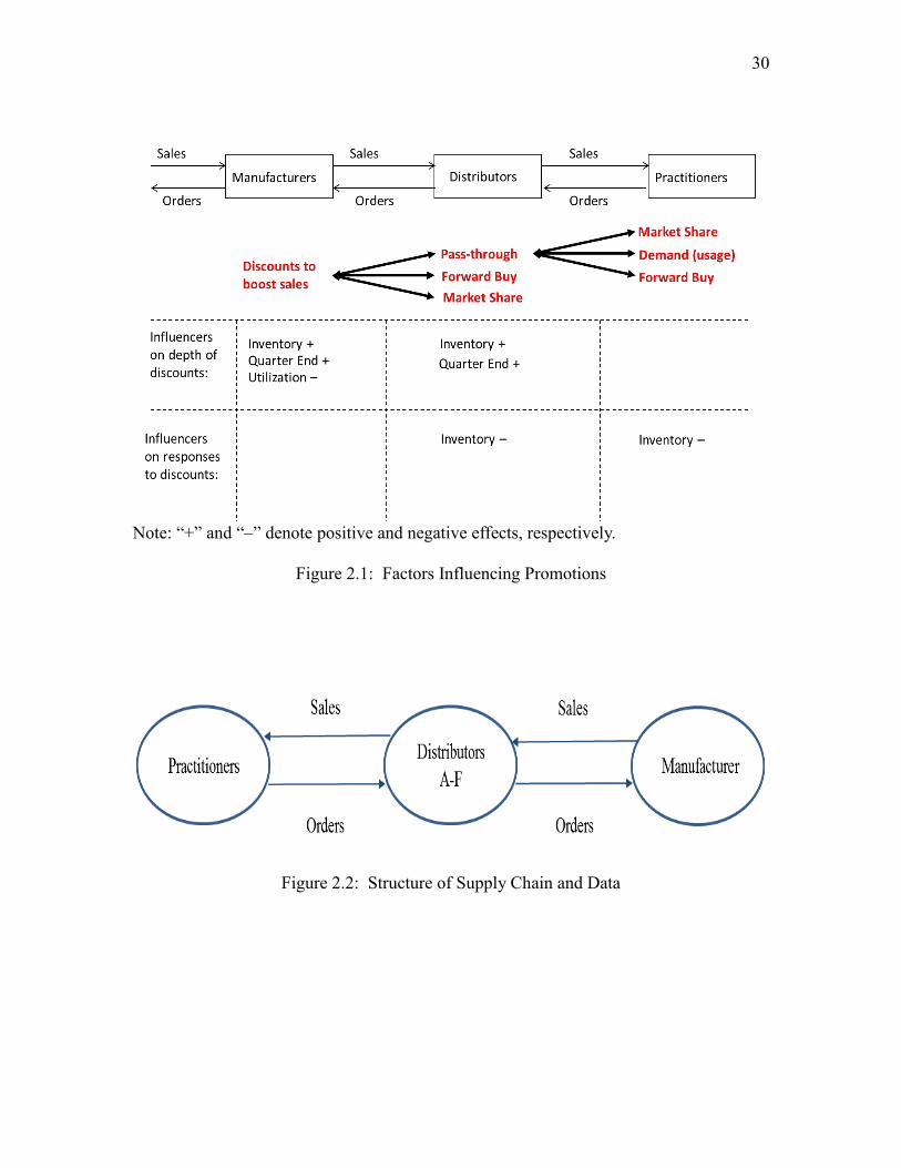
three-echelon supply chain respond to manufacturer’s price discounts. Figure 2.1 shows
factors that influence the offering of discounts and the response to the discounts. We discuss
these factors below from the perspective of manufacturer, distributor, and practitioner,
respectively.
The Manufacturer’s Perspective: The main reason that a manufacturer offers a
discount is to increase sales volume. The willingness of a manufacturer to run trade
promotions depends on several factors. The first one is inventory. When a manufacturer is
burdened with excess inventory, there are many financial drawbacks such as increased
holding cost, reduced profits, and adverse impact on cash flow. The manufacturer can use
promotions to liquidate excess inventory and shift inventory holding cost to the distributors
(Cui et al., 2008). The more inventory the manufacturer holds, the more likely it offers
discounts. Inventory positively affects the manufacturer’s offering of a discount. The
second factor is financial report’s timing (end of the fiscal quarter). Managers may take
various actions (e.g., temporary price reductions) to boost sales prior to the end of the fiscal
quarter to meet sales target or earnings benchmarks. Graham et al. (2005) find that 78% of
400 managers surveyed admit to take economic actions that sacrifice long-term value to
manage earnings. Roychowdhury (2006) find that managers choose operational activities
to manipulate earnings to meet earnings thresholds, so promotions have a positive
relationship with the fiscal quarter end. We expect to see that sales are higher at the end of
the fiscal quarter (hockey stick phenomenon). The third factor is capacity utilization. Low
capacity utilization incurs higher fixed costs per unit, and therefore reduces profit. It

16
indicates that there is a lack of market demand and portrays a negative image of
management. When experiencing low capacity utilization, the manufacturer will be more
likely to offer promotions to stimulate demand in order to keep the utilization at the
appropriate level. Promotions have a negative association with capacity utilization.
The Distributor’s Perspective: The distributor responds to promotions in three ways.
First, the distributor will purchase from manufactures who provide promotions rather than
from competing manufacturers who do not. This affects manufacturers’ market share:
Market share of manufacturers who offer discounts increases, and that of those who do not
decreases. Second, since the purpose of the trade promotion is to get the distributor to offer
the practitioners a price discount and therefore increase sales, the distributor will pass
through (some) promotions and increase its inventories in anticipation of increased sales
to practitioners. Third, the distributor will forward buy and hold inventory in order to take
advantage of the discounts and save purchasing cost. Forward buying benefits the
distributor at the expense of the manufacturer: The distributor buys at reduced costs, but
the manufacturer has a lower sales revenue because there is no overall increase in
practitioner demand to compensate for the discounted price. In any of three cases
aforementioned, trade promotions increase orders placed by the distributor. When a
distributor decides how much to order in each period to meet demand for its products,
inventory on hand must be taken into account. Higher inventory level causes the distributor
to order less to avoid additional holding cost. The distributor evaluates trade-off between
savings from the promotion and extra inventory costs. The distributor’s inventory
negatively affects its response to the discount. As in the manufacturer’s case, the
distributor’s willingness to provide practitioners with discounts depends on inventory and
17
fiscal quarter end. The distributor’s inventory positively affects the distributor’s own
offering of a discount, as does the distributor’s own fiscal quarter end.
The Practitioner’s Perspective: When distributors pass through trade promotions to
the practitioners or offer practitioners their own promotions, the practitioners react in the
following three ways: First, they purchase from distributors who provide discounts rather
than from those who do not. This causes distributors’ market share to shift. Second, the
practitioners may purchase more units than usual and consume them at a higher rate.
Consumption responds to promotions because promotions have the ability to increase
practitioners’ inventory level. Higher inventory levels mean fewer stockouts. The
practitioners have more chances to consume the product. Both behavioral and economic
theory provide supporting evidence that high inventory can increase usage rate (Ailawadi
& Neslin, 1998). Third, the practitioners may forward buy. As in the distributor’s case, the
practitioner’s inventory negatively affects its response to the distributor’s discount.
The second objective of this chapter is to investigate the impact of trade promotions.
Trade promotion is identified as a cause of the bullwhip effect (Lee et al. 1997a). We
empirically test whether the bullwhip effect exists. If so, how severe is the effect? We also
calculate the financial cost of the bullwhip effect. Following the original definition of the
bullwhip effect by Lee et al. (1997a), we define
𝐵𝑢𝑙𝑙𝑤ℎ𝑖𝑝 𝑅𝑎𝑡𝑖𝑜 =
𝑉[𝑂𝑟𝑑𝑒𝑟]
𝑉[𝐷𝑒𝑚𝑎𝑛𝑑] (2.1)
where 𝑉[ ] is the variance operator. The numerator and denominator are the variance of
order series and demand series of a single product. Order can be interpreted as production
in manufacturing setting. We say that the bullwhip effect is exhibited by a product when
the ratio is greater than 1. Given that trade promotion is recognized as a source of the
18
bullwhip effect, we expect that bullwhip ratio is greater than 1 for products that receive
promotions.
2.4 Empirical Context and Data
Our empirical analysis is based on a proprietary dataset in the healthcare industry.
The dataset consists of one manufacturer and six nation-wide distributors (A-F). The
structure of the supply chain and of the data is shown in Figure 2.2. The manufacturer
produces consumable products that all medical practitioners in this specialty use, and has
a lion’s share of the market. These products are applied to patients in medical practitioner’s
office and have a shelf life of approximately 18 months. The manufacturer may periodically
offer price discounts to its distributors to meet sales targets, for example, at the end of the
manufacturer’s fiscal quarter. In turn, a distributor may pass through some of the discounts
to its customers. Also the distributor may offer its own promotions to meet sales targets at
the end of its fiscal quarter.
We collect monthly data on 31 stock keeping units (SKUs) over the period between
January 2010 and June 2014. The frequency of the data (monthly) matches the frequency
of decisions by the manufacturer and distributors, so the data do not have the “time-
disaggregation bias” identified by Kahn (1992), and are suitable for appropriate supply
chain cost assessment (Chen & Lee, 2012). The entire product category is made up of these
31 SKUs. Specifically, the following data are used to perform empirical analysis:
manufacturer’s production, manufacturer’s sales (shipments to distributors), distributors’
orders, distributors’ sales, manufacturer’s wholesale price, and manufacturer’s price
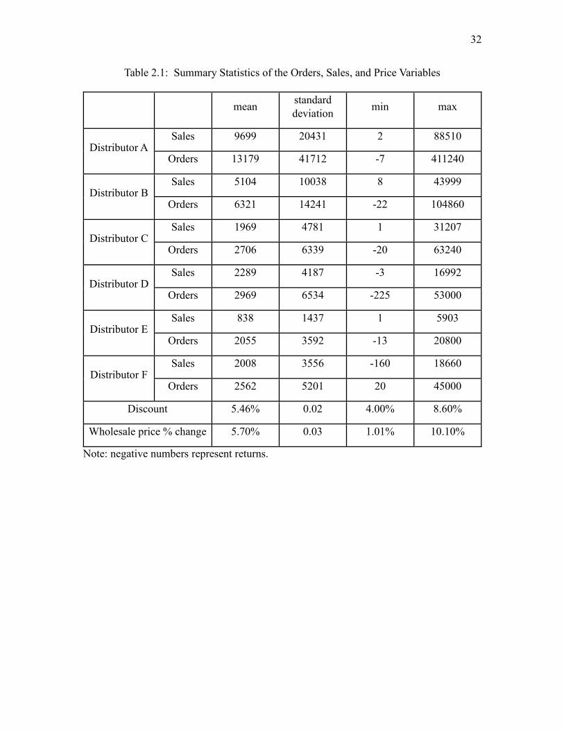
discounts. Table 2.1 presents summary statistics by distributor for the orders, sales, and

19
price variables used in our study. SKUs 1-11 are carried by all distributors. SKUs 12-15,
16-19, 20-23, 24-26, 27-28, and 29-31 are carried only by distributors A-F, respectively.
Manufacturer offers price discounts for 2 SKUs (SKUs 1 and 2), which account for 40%
of the total sales. All 31 SKUs have annual wholesale price increase. Quantities are
expressed in physical units rather than dollar amounts. This avoids measurement and
accounting problems associated with inventory evaluation (Lai, 2005). Over the entire
sample period, manufacturer offers ten discounts, five discounts, four discounts, four
discounts, five discounts, and six discounts to distributors A-F, respectively. Among these
thirty-four discounts, twenty-five occur at the end of manufacturer’s fiscal quarter.
We do not have access to distributors’ inventory data, so an estimate of inventories
is made using the following relationship:
𝐼𝑛𝑣𝑒𝑛𝑡𝑜𝑟𝑦𝑡 = 𝐼𝑛𝑣𝑒𝑛𝑡𝑜𝑟𝑦𝑡−1 + 𝑃𝑟𝑜𝑑𝑢𝑐𝑡𝑖𝑜𝑛𝑡 − 𝑆𝑎𝑙𝑒𝑠𝑡 (2.2)
where 𝐼𝑛𝑣𝑒𝑛𝑡𝑜𝑟𝑦𝑡 denotes the net inventories at the end of period 𝑡. We use shipments
received from manufacturer as a proxy for distributor’s production. Since initial inventories
are not available, we choose them so that each period’s inventory is greater than or equal
to zero. Thus, the inventory data used in model estimation are relative inventory. Blattberg
and Levin (1987) use the same approach to set the starting inventory.
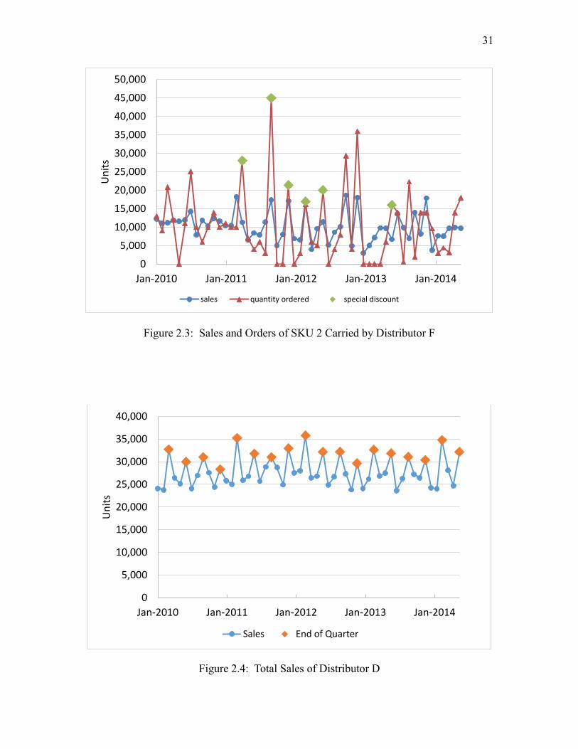
Figure 2.3 shows sales and orders of a distributor for a specific product. We observe
that there are usually troughs in orders after a price discount ends, suggesting forward
buying on the part of the distributor during the promotional period. If the distributor passes
promotions on to practitioners, the sales pattern and order pattern will be close to each
other. In Figure 2.3, the sales of the distributor have much less variability than the orders
placed by the distributor. This implies that the distributor is buying for inventory and passes

20
only some portion of the promotions on to practitioners. Figure 2.4 shows the total sales of
a distributor. We see spikes towards the end of every quarter. Hockey stick phenomenon is
prevalent.
2.5 Model Specification
In order to explore the impact of trade promotions and identify the presence or
absence of the hockey stick effect, we propose four empirical models and describe them in
detail below. Recall that manufacturer provides price discounts only for SKUs 1 and 2,
which carried by all distributors, and some of the other 29 SKUs are not carried by every
distributor. We analyze SKUs 1 and 2 separately from the remaining 29 SKUs. Specifically,
Models I(a), I(b), and III apply to SKUs 1 and 2, and Models II and IV apply to SKUs 3-
31.
2.5.1 Distributor Order Model
We regress the distributors’ orders on explanatory variables with the following
specification (Model I(a)) for SKUs 1 and 2:
𝑂𝑟𝑑𝑒𝑟𝑠𝑖𝑡 = 𝛼𝑖 + 𝛽1𝑡 + 𝛽2𝑊ℎ𝑜𝑙𝑒𝑠𝑎𝑙𝑒𝑖𝑡 + 𝛾𝑖𝐷𝑖𝑠𝑐𝑜𝑢𝑛𝑡𝑖𝑡
+ 𝛿𝑖(𝐿𝑎𝑔𝑔𝑒𝑑 𝐼𝑛𝑣𝑒𝑛𝑡𝑜𝑟𝑦)𝑖𝑡 + 휀𝑖𝑡
(2.3)
where 𝑖 and 𝑡 refer to distributor and time, respectively. 𝑂𝑟𝑑𝑒𝑟𝑠𝑖𝑡 is the orders placed by
distributor 𝑖 in month 𝑡 to the manufacturer. 𝛼𝑖 is the time-invariant distributor-specific
fixed effect for distributor 𝑖. 𝑡 is a linear time trend. That is, 𝑡 is 1 in the first month, 2 in
the second month, and up to 54 in the last month. Manufacturer increases wholesale price
once per year. When manufacturer increases price, what typically happens is that it sends
21
out the price change notice 60 days before effective date and then distributors will react
accordingly. For example, if the manufacturer plans for a January price increase,
distributors may make a purchase in December, depending on how big the price increase
is. A price increase is often preceded by an increase in orders. This can be modeled by
having a dummy variable for the periods prior to the price increase times the percentage
price changes. More specifically, if there is a 10% wholesale price increase for distributor
𝑖 in July, 𝑊ℎ𝑜𝑙𝑒𝑠𝑎𝑙𝑒𝑖𝑡 will be 0 for July and 10% for May and June. To represent the
magnitude of a promotion, 𝐷𝑖𝑠𝑐𝑜𝑢𝑛𝑡𝑖𝑡 is a percentage dollar discount for distributor 𝑖 in
month 𝑡. This percentage discount makes various trade promotions comparable over time.
Since trade promotions increase orders, we expect 𝛾𝑖 to be positive.
(𝐿𝑎𝑔𝑔𝑒𝑑 𝐼𝑛𝑣𝑒𝑛𝑡𝑜𝑟𝑦)𝑖𝑡 is one period lagged inventory for distributor 𝑖 in month 𝑡 .
Distributors usually use some form of inventory model to determine how much to order on
a given promotion. We include lagged inventories in the model because last period’s
inventories influence the quantity to order in the present period. Inventories inversely affect
orders, so 𝛿𝑖 is expected to have a negative sign. 휀𝑖𝑡 denotes the error term, which account
for all of the order fluctuations that we cannot explain.
In order to demonstrate the robustness of the results from Model I(a), we estimate
the alternative model specification for each distributor and product combination (Model
I(b)):
𝑂𝑟𝑑𝑒𝑟𝑠𝑡 = α + 𝛽1𝑡 + 𝛽2𝑊ℎ𝑜𝑙𝑒𝑠𝑎𝑙𝑒𝑡 + γ𝐷𝑖𝑠𝑐𝑜𝑢𝑛𝑡𝑡
+ δ(𝐿𝑎𝑔𝑔𝑒𝑑 𝐼𝑛𝑣𝑒𝑛𝑡𝑜𝑟𝑦)𝑡 + 휀𝑡
(2.4)
Since not every distributor carries SKUs 3-31, we analyze each distributor and
product combination separately by running the following regression model (Model II):
22
𝑂𝑟𝑑𝑒𝑟𝑠𝑡 = α + 𝛽1𝑡 + 𝛽2𝑊ℎ𝑜𝑙𝑒𝑠𝑎𝑙𝑒𝑡 + 𝛿(𝐿𝑎𝑔𝑔𝑒𝑑 𝐼𝑛𝑣𝑒𝑛𝑡𝑜𝑟𝑦)𝑡
+ 휀𝑡
(2.5)
2.5.2 Distributor Sales Model
We perform regression analysis on distributors’ sales using the following linear
specification (Model III) for SKUs 1 and 2:
𝑆𝑎𝑙𝑒𝑠𝑖𝑡 = 𝛼𝑖 + 𝛽1𝑡 + 𝛽2𝑊ℎ𝑜𝑙𝑒𝑠𝑎𝑙𝑒𝑖𝑡 + 𝛿𝑖(𝑄𝑢𝑎𝑟𝑡𝑒𝑟𝐸𝑛𝑑)𝑖𝑡
+ 𝛾𝑖𝐷𝑖𝑠𝑐𝑜𝑢𝑛𝑡𝑖𝑡 + 휀𝑖𝑡
(2.6)
where 𝑖 and 𝑡 refer to distributor and time, respectively. 𝑆𝑎𝑙𝑒𝑠𝑖𝑡 is the sales of distributor 𝑖
to practitioners in month 𝑡. 𝑊ℎ𝑜𝑙𝑒𝑠𝑎𝑙𝑒𝑖𝑡 is exactly the same as in Model I(a). Since we do
not know distributors’ pricing information, we use manufacturer’s annual wholesale price
increase as a proxy for distributor’s wholesale price change. (𝑄𝑢𝑎𝑟𝑡𝑒𝑟𝐸𝑛𝑑)𝑖𝑡 is a dummy
variable that equals one if the sales occur at the last month of a fiscal quarter and zero
otherwise. We assume that the fiscal effects are the same in the first and second months of
a fiscal quarter and use these as the base months. 𝛿𝑖 measures the amount by which
distributor 𝑖’s unit sales change, holding other factors constant, from the first two months
of a fiscal quarter to the third one. If hockey stick phenomenon exists, 𝛿𝑖 is expected to
have a positive sign.
Ideally, 𝐷𝑖𝑠𝑐𝑜𝑢𝑛𝑡𝑖𝑡 is a percentage dollar discount offered by distributor 𝑖 in month
𝑡 . Given that we do not collect information about distributor promotions, we use
manufacturer promotions as a surrogate for distributor promotions. Since discounts may
increase sales, 𝛾𝑖 is expected to have a positive sign.
For SKUs 3-31 that are not carried by all distributors, we run separate regressions
23
for each distributor and product combination (Model IV):
𝑆𝑎𝑙𝑒𝑠𝑡 = 𝛼 + 𝛽1𝑡 + 𝛽2𝑊ℎ𝑜𝑙𝑒𝑠𝑎𝑙𝑒𝑡 + 𝛿(𝑄𝑢𝑎𝑟𝑡𝑒𝑟𝐸𝑛𝑑)𝑡 + 휀𝑡 (2.7)
The data used in analysis are stationary because the Dickey-Fuller test suggests that
there is no unit root in each data series. Since our data contain observations across
distributors and months, it is likely that the variance of errors varies across distributors and
errors for different observations are correlated within a distributor. We estimate Models I(a)
and III by fixed effect (FE) method with cluster-robust standard errors that are robust to
arbitrary heteroskedasticity and arbitrary serial correlation (see Wooldridge, 2010, Chapter
10). We estimate Models I(b), II, and IV by ordinary least squares (OLS) with Newey-West
standard errors (see Greene, 2008, Chapter 19). The error structure is assumed to be
heteroskedastic and AR(1) autocorrelated.
2.6 Results
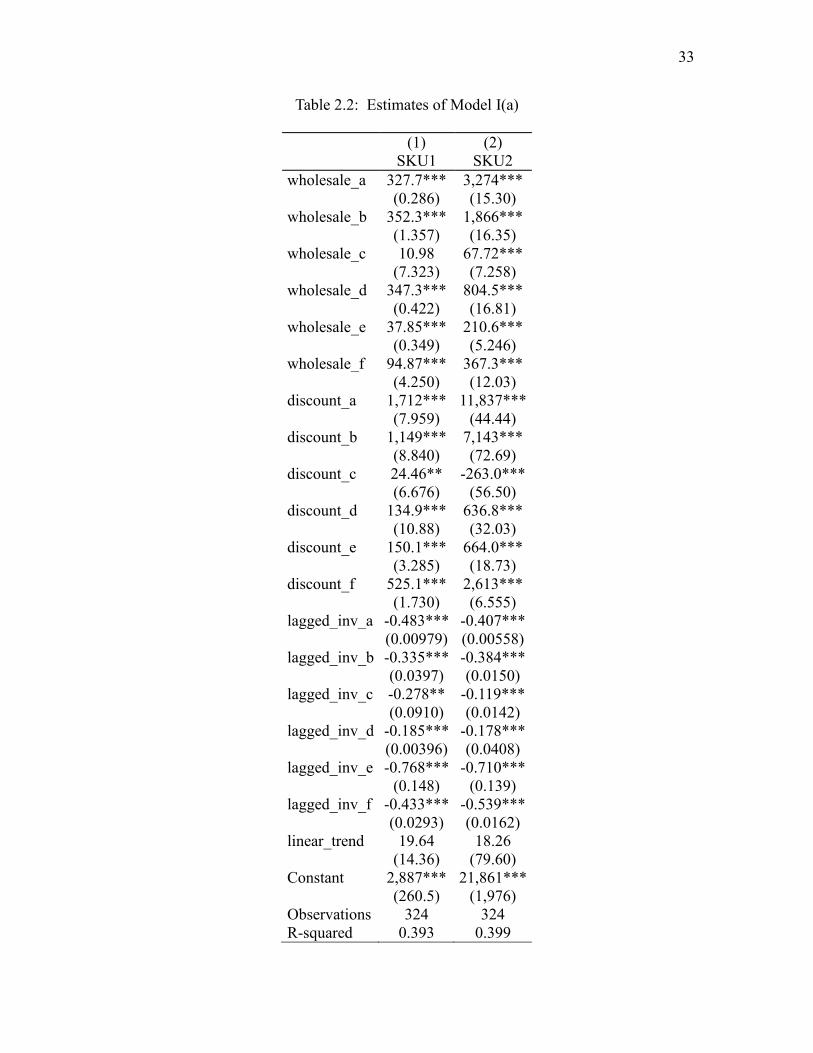
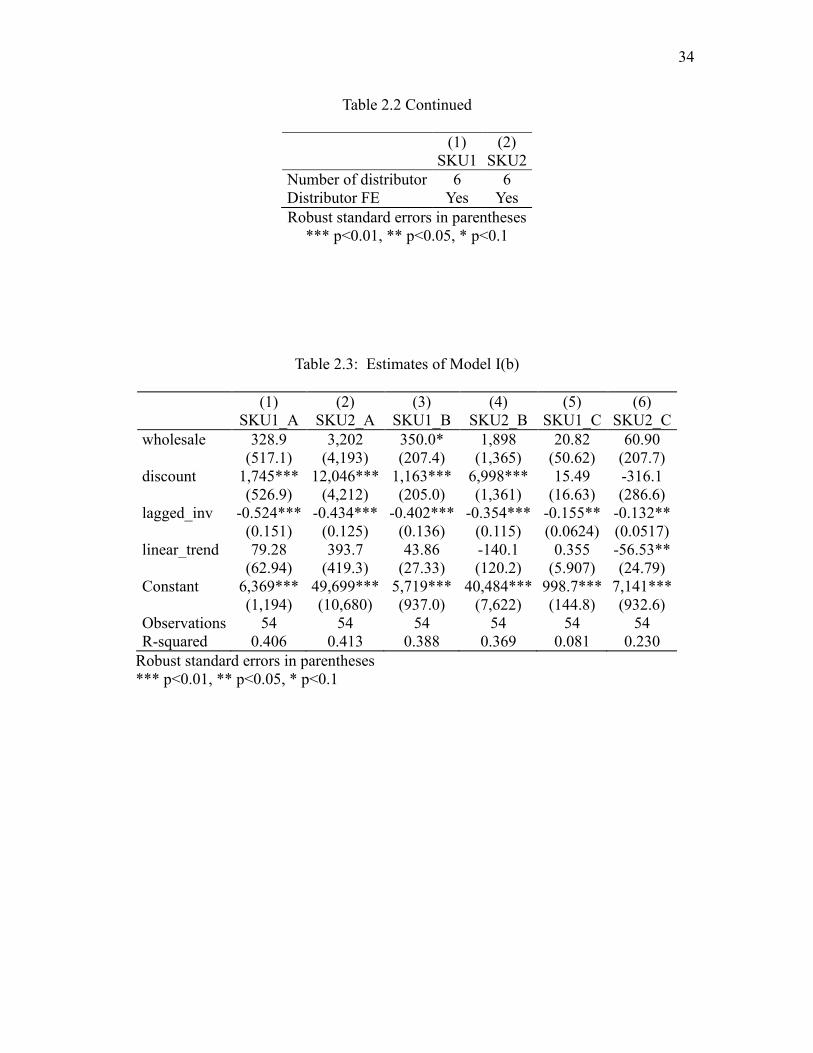
In Tables 2.2 and 2.3, we report estimates of Models I(a) and I(b). Among these two
models, the coefficients on 𝐷𝑖𝑠𝑐𝑜𝑢𝑛𝑡 for distributors A, B, E, and F are positive and
statistically significant across products, indicating that distributors A, B, E, and F place a
significantly larger order during promotional period. While these distributors seem to
behave consistently with distributors described in previous literature (i.e., wholesaler or
retailer increases its orders placed to the manufacturer when a trade promotion is offered
(e.g., Srinivasan et al., 2004)), other distributors do not. Specifically, the coefficients on
𝐷𝑖𝑠𝑐𝑜𝑢𝑛𝑡 for distributors C and D have varying signs and different levels of significance
across models. Clearly, not all distributors respond to the price discounts. The coefficients
on 𝐿𝑎𝑔𝑔𝑒𝑑 𝐼𝑛𝑣𝑒𝑛𝑡𝑜𝑟𝑦 for all distributors are negative and statistically significant across

24
products in two models, indicating that higher inventory level is associated with lower
order quantity. This is consistent with our expectation: Inventory inversely affects order.
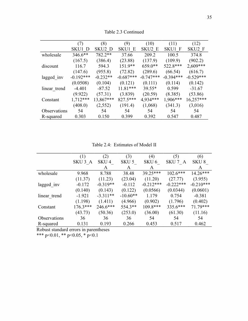
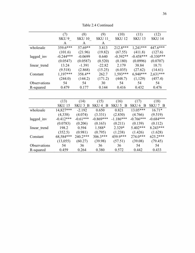
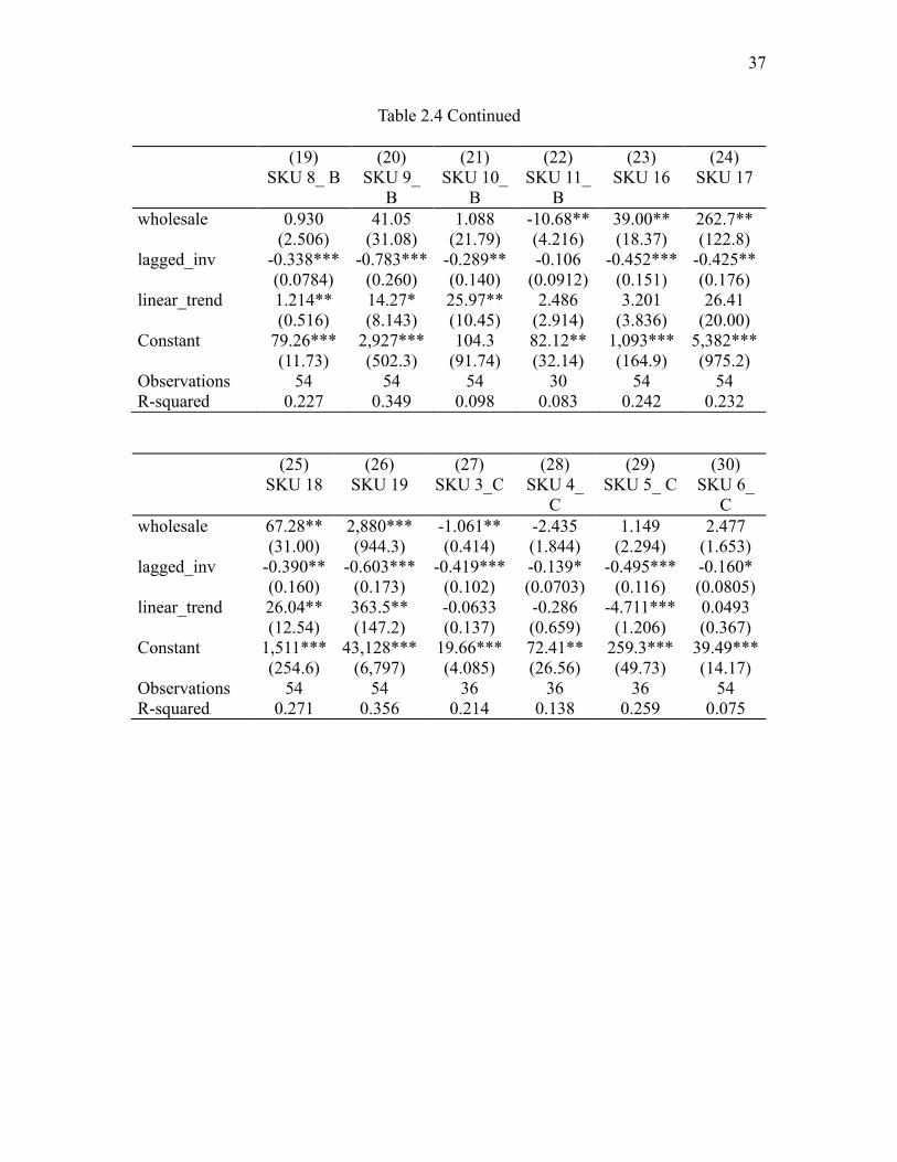
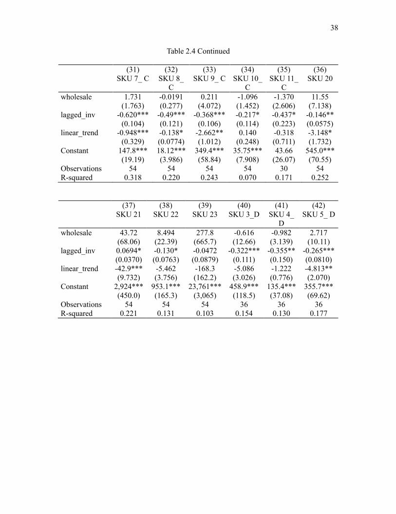
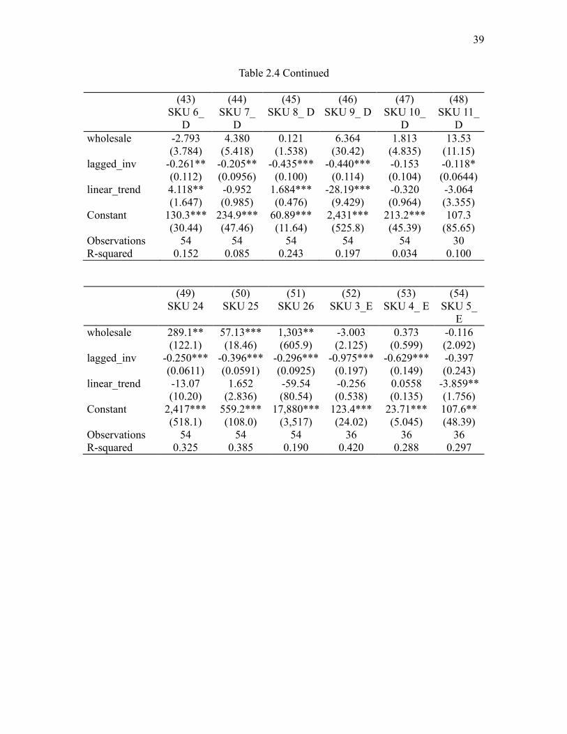
Estimates of Model II are shown in Table 2.4. The coefficients on 𝑊ℎ𝑜𝑙𝑒𝑠𝑎𝑙𝑒 are
positive and statistically significant for almost all products carried by distributor A, but not
for products carried by other distributors. Only distributor A responds to wholesale price
increase. In general, the coefficients on 𝐿𝑎𝑔𝑔𝑒𝑑 𝐼𝑛𝑣𝑒𝑛𝑡𝑜𝑟𝑦 are negative and statistically
significant, indicating that inventory is negatively associated with orders.
Table 2.5 shows estimates of Model III. Columns (1)-(3) and (4)-(6) are for SKU 1
and SKU 2, respectively. In columns (1) and (4), the coefficients on 𝐷𝑖𝑠𝑐𝑜𝑢𝑛𝑡 are positive
and statistically significant for distributor F, indicating that distributor F has significantly
higher sales for SKUs 1 and 2 during manufacturer promotion period. This implies that
distributor F passes through trade promotions to practitioners. But we do not know the
pass-through rate. Orders placed by practitioners to distributors and shipments from
distributors to practitioners may occur in different months. Given that we only have
shipments data, it is likely that some distributors pass through trade promotions, but the
shipments occur in the next month rather than in the same month as manufacturer
promotions. In columns (2) and (5), we use one period lagged discount variable. The
coefficients on this variable are positive and statistically significant for distributors A and
B. These two distributors have significantly higher sales for SKUs 1 and 2 one month later
after manufacturer promotions. This implies that distributors A and B probably pass
through trade promotions. In columns (3) and (6), we use lagged discount for distributors
A and B, and use discount for the remaining distributors. The results show that distributors
A, B, and F may pass through promotions for SKUs 1 and 2. Across columns (1)-(6), the
25
coefficients on 𝑄𝑢𝑎𝑟𝑡𝑒𝑟𝐸𝑛𝑑 are positive and statistically significant for distributors B, C,
D, E, and F. The hockey stick effect exists at most distributors. If we compare the
coefficients on 𝐷𝑖𝑠𝑐𝑜𝑢𝑛𝑡 for distributors A, B, E, and F in Model I(a) with those in Model
III, we find that the magnitude of the coefficients in Model I(a) is much larger than that in
Model III, indicating that most of the incremental units sold by the manufacturer during
promotion period are not the incremental units sold by distributors. Distributors A, B, E,
and F forward buy and build inventories at lower costs when trade promotions occur. The
distributors pocket the discount promotions without passing the benefits to the practitioners
or with passing through a small part of the benefits. This result is consistent with the
findings in the literature that trade promotions are not profitable for manufacturers (e.g.,
Abraham & Lodish, 1990).
Parameter estimates of Model IV are reported in Table 2.6. The coefficients on
𝑄𝑢𝑎𝑟𝑡𝑒𝑟𝐸𝑛𝑑 are positive and statistically significant for 10 out of 13 products carried by
distributor B and 7 out of 12 products carried by distributor D. The coefficients on
𝑄𝑢𝑎𝑟𝑡𝑒𝑟𝐸𝑛𝑑 are positive but not significant for the remaining 5 products carried by
distributor D. These results indicate that distributors B and D have higher sales in the last
month of a fiscal quarter than they do in the first two months.
In Table 2.7, we report the bullwhip ratios. The bullwhip ratio for the manufacturer
is equal to variance in production stream divided by variance in demand stream. Since we
do not have distributors’ demand data, we use sales as a proxy for demand. This will not
inflate bullwhip estimates because distributors in our dataset usually carry enough
inventory and stockouts rarely occur. The bullwhip ratio for distributors is equal to variance
in order stream divided by variance in sales stream. At the SKU level, the substantial
26
bullwhip effect exists at each distributor. The average ratio is 49.81 (ranging from 3.85 to
216.97), much higher than those reported in the previous literature. However, the bullwhip
effect is not exhibited by manufacturer, indicating that the manufacturer makes production
smoother than demand. This result is aligned well with production smoothing hypothesis.
Our findings are consistent with those obtained by Cachon et al. (2007) at industry level.
Many firms use market share as a key indicator of their relative success in market
competitiveness. From the information we collect from several distributors, we know that
the distribution of health care products is highly competitive and these distributors actually
compete with each other. The product category in our dataset is mature and the primary
demand doesn’t increase over sample periods. If a distributor passes through trade
promotions to practitioners or boosts sales at the quarter end, its market share will increase.
Table 2.8 presents the correlation coefficients between distributors’ market share and trade
promotion. There is a significant positive association between market share of distributors
B and F and manufacturer’s discounts for SKUs 1 and 2. This implies that distributors B
and F probably pass through trade promotions. The result is consistent with that from
Model III. In Table 2.9, we report the correlation coefficients between distributors’ market
share and their fiscal quarter ends. Market share of distributors B, D, and F has a
significantly positive relationship with fiscal quarter ends for SKUs 1 and 2. This result is
consistent with the hockey stick effect identified in Model III.
Trade promotions cause forwarding buying, which inflates inventories and
therefore raises certain costs. We seek to estimate the added inventory costs resulting from
promotions for manufacturer and distributors. In order to do this, we need to compare the
actual inventories with those (hypothetical inventories) that would be carried if there was
27
no promotion. When calculating the hypothetical inventory, we assume that manufacturer
and distributors implement base stock inventory model (also called the order-up-to model)
and maintain 99% service level. From our interviews with management of the manufacturer
and public information of several distributors, we think these assumptions are reasonable
approximations to real life situations. By using the analytical model developed by
Moinzadeh (1997), we estimate that the carrying costs on inventories that include storage,
insurance, handling, and capital charges are about 15% per year. We use Model III to
forecast what the distributors’ sales would have been in the absence of the discounts. Then
we calculate the hypothetical inventory level at distributors and manufacturer. Table 2.10
shows the yearly added costs caused by promotions. The cost to the manufacturer is over
one million dollars and represents 3.21% of total sales of the products affected. The costs
to several distributors represent more than 1% of total sales. The cost to the supply chain
is about two million dollars. Moreover, these substantial amounts account for only a part
of the total costs of trade promotions. We do not try to quantify other expenses such as
higher administrative and selling costs to operate increasingly complex procurement and
sales programs, the costs of the time spent on design and evaluation of trade deals, and
higher production costs due to uneven scheduling. These costs of promotions may equal or
exceed the costs that we have estimated. Trade promotions incur high costs for both
manufacturer and distributors and impair the efficiency of the supply chain.
2.7 Conclusion
Trade promotions are the most important promotional tool for manufacturers. It is
reported in A.C. Nielsen 2002 Trade Promotion Practices Study that trade promotion

28
spending accounts for 16% of gross sales. Conventional wisdom in marketing holds that
(1) trade promotions are the main culprit behind retailer forwarding buying and (2)
manufacturers are hurt by forward buying. Our results are consistent with this wisdom. By
using a proprietary dataset in the healthcare industry, we find that some distributors do
forward buy when offered wholesale price discounts and pass through only a small part of
discounts to practitioners, causing trade promotions not to pay for manufacturers. Given
the huge expenditure on trade promotions, we encourage marketing managers to re-
examine the components of their promotion programs. In fact, our discussions with
managers of the manufacturer reveal that they are suspicious of the effectiveness of
periodic discounts and plan to implement a new pricing scheme that excludes the discounts.
To the best of our knowledge, our study is the first empirical study on the effects of trade
promotions for health care products.
We observe hockey stick phenomenon at the manufacturer and several distributors.
The resulting sales surge causes substantial difficulty in production planning,
transportation, and inventory management. Both trade promotion and hockey stick
phenomenon contribute to triggering the bullwhip effect, which is one of the most harmful
problems in the supply chain management. We find that all distributors exhibit an intensive
bullwhip effect, lowering supply chain efficiency. One leading cause of the hockey stick
phenomenon is salesperson and executive compensation contracts, which induce these
agents to manipulate prices and influence the timing of sales. Our results provide practicing
managers with a good starting point to think about their incentive schemes.
Since there are only two products in our dataset that receive price discounts, this
limits the generalizability of our findings to the larger class of products. We do not collect

29
information about distributor promotions, so we have to use an alternative variable as a
measure of distributor activity. The availability of distributor promotion data in the future
will enhance the models developed in this chapter and give more accurate model estimates.
30
Note: “+” and “–” denote positive and negative effects, respectively.
Figure 2.1: Factors Influencing Promotions
Figure 2.2: Structure of Supply Chain and Data
31
Figure 2.3: Sales and Orders of SKU 2 Carried by Distributor F
Figure 2.4: Total Sales of Distributor D
0
5,000
10,000
15,000
20,000
25,000
30,000
35,000
40,000
45,000
50,000
Jan-2010 Jan-2011 Jan-2012 Jan-2013 Jan-2014
Un
its
sales quantity ordered special discount
0
5,000
10,000
15,000
20,000
25,000
30,000
35,000
40,000
Jan-2010 Jan-2011 Jan-2012 Jan-2013 Jan-2014
Un
its
Sales End of Quarter
32
Table 2.1: Summary Statistics of the Orders, Sales, and Price Variables
mean standard
deviation min max
Distributor A Sales 9699 20431 2 88510
Orders 13179 41712 -7 411240
Distributor B Sales 5104 10038 8 43999
Orders 6321 14241 -22 104860
Distributor C Sales 1969 4781 1 31207
Orders 2706 6339 -20 63240
Distributor D Sales 2289 4187 -3 16992
Orders 2969 6534 -225 53000
Distributor E Sales 838 1437 1 5903
Orders 2055 3592 -13 20800
Distributor F Sales 2008 3556 -160 18660
Orders 2562 5201 20 45000
Discount 5.46% 0.02 4.00% 8.60%
Wholesale price % change 5.70% 0.03 1.01% 10.10%
Note: negative numbers represent returns.
33
Table 2.2: Estimates of Model I(a)
(1) (2)
SKU1 SKU2
wholesale_a 327.7*** 3,274***
(0.286) (15.30)
wholesale_b 352.3*** 1,866***
(1.357) (16.35)
wholesale_c 10.98 67.72***
(7.323) (7.258)
wholesale_d 347.3*** 804.5***
(0.422) (16.81)
wholesale_e 37.85*** 210.6***
(0.349) (5.246)
wholesale_f 94.87*** 367.3***
(4.250) (12.03)
discount_a 1,712*** 11,837***
(7.959) (44.44)
discount_b 1,149*** 7,143***
(8.840) (72.69)
discount_c 24.46** -263.0***
(6.676) (56.50)
discount_d 134.9*** 636.8***
(10.88) (32.03)
discount_e 150.1*** 664.0***
(3.285) (18.73)
discount_f 525.1*** 2,613***
(1.730) (6.555)
lagged_inv_a -0.483*** -0.407***
(0.00979) (0.00558)
lagged_inv_b -0.335*** -0.384***
(0.0397) (0.0150)
lagged_inv_c -0.278** -0.119***
(0.0910) (0.0142)
lagged_inv_d -0.185*** -0.178***
(0.00396) (0.0408)
lagged_inv_e -0.768*** -0.710***
(0.148) (0.139)
lagged_inv_f -0.433*** -0.539***
(0.0293) (0.0162)
linear_trend 19.64 18.26
(14.36) (79.60)
Constant 2,887*** 21,861***
(260.5) (1,976)
Observations 324 324
R-squared 0.393 0.399
34
Table 2.2 Continued
(1) (2)
SKU1 SKU2
Number of distributor 6 6
Distributor FE Yes Yes
Robust standard errors in parentheses
*** p<0.01, ** p<0.05, * p<0.1
Table 2.3: Estimates of Model I(b)
(1) (2) (3) (4) (5) (6)
SKU1_A SKU2_A SKU1_B SKU2_B SKU1_C SKU2_C
wholesale 328.9 3,202 350.0* 1,898 20.82 60.90
(517.1) (4,193) (207.4) (1,365) (50.62) (207.7)
discount 1,745*** 12,046*** 1,163*** 6,998*** 15.49 -316.1
(526.9) (4,212) (205.0) (1,361) (16.63) (286.6)
lagged_inv -0.524*** -0.434*** -0.402*** -0.354*** -0.155** -0.132**
(0.151) (0.125) (0.136) (0.115) (0.0624) (0.0517)
linear_trend 79.28 393.7 43.86 -140.1 0.355 -56.53**
(62.94) (419.3) (27.33) (120.2) (5.907) (24.79)
Constant 6,369*** 49,699*** 5,719*** 40,484*** 998.7*** 7,141***
(1,194) (10,680) (937.0) (7,622) (144.8) (932.6)
Observations 54 54 54 54 54 54
R-squared 0.406 0.413 0.388 0.369 0.081 0.230
Robust standard errors in parentheses
*** p<0.01, ** p<0.05, * p<0.1
35
Table 2.3 Continued
(7) (8) (9) (10) (11) (12)
SKU1_D SKU2_D SKU1_E SKU2_E SKU1_F SKU2_F
wholesale 346.6** 782.2** 37.66 209.2 100.5 374.8
(167.5) (386.4) (23.88) (137.9) (109.9) (902.2)
discount 116.7 594.3 151.9** 659.0** 522.8*** 2,609***
(147.6) (955.8) (72.82) (289.6) (66.54) (616.7)
lagged_inv -0.192*** -0.232** -0.687*** -0.747*** -0.394*** -0.529***
(0.0508) (0.104) (0.121) (0.111) (0.114) (0.142)
linear_trend -4.401 -87.52 11.81*** 39.55* 0.599 -31.67
(9.922) (57.31) (3.839) (20.59) (8.385) (53.86)
Constant 1,712*** 13,867*** 827.5*** 4,934*** 1,906*** 16,257***
(408.0) (2,552) (191.4) (1,068) (341.3) (3,016)
Observations 54 54 54 54 54 54
R-squared 0.303 0.150 0.399 0.392 0.547 0.487
Table 2.4: Estimates of Model II
(1) (2) (3) (4) (5) (6)
SKU 3_A SKU 4_
A
SKU 5_
A
SKU 6_
A
SKU 7_ A SKU 8_
A
wholesale 9.968 8.788 38.48 39.25*** 102.6*** 14.26***
(11.37) (11.23) (23.04) (11.20) (27.77) (3.955)
lagged_inv -0.172 -0.319** -0.112 -0.212*** -0.222*** -0.210***
(0.140) (0.143) (0.122) (0.0566) (0.0344) (0.0601)
linear_trend -1.921 -3.311** -10.60** 1.179 0.754 -0.381
(1.198) (1.411) (4.966) (0.902) (1.796) (0.402)
Constant 176.3*** 246.6*** 554.3** 109.8*** 335.6*** 71.79***
(43.73) (50.36) (253.0) (36.00) (61.30) (11.16)
Observations 36 36 36 54 54 54
R-squared 0.131 0.193 0.266 0.453 0.517 0.462
Robust standard errors in parentheses
*** p<0.01, ** p<0.05, * p<0.1
36
Table 2.4 Continued
(7) (8) (9) (10) (11) (12)
SKU 9_
A
SKU 10_
A
SKU 11_
A
SKU 12 SKU 13 SKU 14
wholesale 359.6*** 57.69** 3.813 212.8*** 1,241*** 447.6***
(101.6) (21.96) (19.82) (67.55) (411.8) (127.6)
lagged_inv -0.244*** -0.0699 0.640 -0.392** -0.458*** -0.330***
(0.0547) (0.0587) (0.520) (0.180) (0.0996) (0.0707)
linear_trend 13.24 -1.391 -22.82 2.179 38.84 18.71
(9.518) (2.868) (15.25) (6.035) (27.62) (14.61)
Constant 1,197*** 358.4** 262.7 1,593*** 6,940*** 2,631***
(244.0) (144.2) (171.2) (448.7) (1,129) (457.4)
Observations 54 54 30 54 54 54
R-squared 0.479 0.177 0.144 0.416 0.432 0.476
(13) (14) (15) (16) (17) (18)
SKU 15 SKU 3_B SKU 4_ B SKU 5_ B SKU 6_ B SKU 7_ B
wholesale 14,827*** -2.192 0.650 0.821 13.05*** 16.71*
(4,338) (4.074) (3.331) (2.830) (4.766) (9.519)
lagged_inv -0.412*** -0.61*** -0.869*** -1.186*** -0.766*** -0.684***
(0.0783) (0.206) (0.163) (0.211) (0.139) (0.112)
linear_trend 198.2 0.594 1.588* 2.329* 5.402*** 8.243***
(352.5) (0.981) (0.795) (1.238) (1.426) (1.628)
Constant 68,584*** 240.2*** 306.3*** 459.9*** 274.0*** 625.2***
(13,055) (60.27) (39.98) (57.51) (39.08) (79.45)
Observations 54 36 36 36 54 54
R-squared 0.459 0.264 0.380 0.572 0.442 0.433
37
Table 2.4 Continued
(19) (20) (21) (22) (23) (24)
SKU 8_ B SKU 9_
B
SKU 10_
B
SKU 11_
B
SKU 16 SKU 17
wholesale 0.930 41.05 1.088 -10.68** 39.00** 262.7**
(2.506) (31.08) (21.79) (4.216) (18.37) (122.8)
lagged_inv -0.338*** -0.783*** -0.289** -0.106 -0.452*** -0.425**
(0.0784) (0.260) (0.140) (0.0912) (0.151) (0.176)
linear_trend 1.214** 14.27* 25.97** 2.486 3.201 26.41
(0.516) (8.143) (10.45) (2.914) (3.836) (20.00)
Constant 79.26*** 2,927*** 104.3 82.12** 1,093*** 5,382***
(11.73) (502.3) (91.74) (32.14) (164.9) (975.2)
Observations 54 54 54 30 54 54
R-squared 0.227 0.349 0.098 0.083 0.242 0.232
(25) (26) (27) (28) (29) (30)
SKU 18 SKU 19 SKU 3_C SKU 4_
C
SKU 5_ C SKU 6_
C
wholesale 67.28** 2,880*** -1.061** -2.435 1.149 2.477
(31.00) (944.3) (0.414) (1.844) (2.294) (1.653)
lagged_inv -0.390** -0.603*** -0.419*** -0.139* -0.495*** -0.160*
(0.160) (0.173) (0.102) (0.0703) (0.116) (0.0805)
linear_trend 26.04** 363.5** -0.0633 -0.286 -4.711*** 0.0493
(12.54) (147.2) (0.137) (0.659) (1.206) (0.367)
Constant 1,511*** 43,128*** 19.66*** 72.41** 259.3*** 39.49***
(254.6) (6,797) (4.085) (26.56) (49.73) (14.17)
Observations 54 54 36 36 36 54
R-squared 0.271 0.356 0.214 0.138 0.259 0.075
38
Table 2.4 Continued
(31) (32) (33) (34) (35) (36)
SKU 7_ C SKU 8_
C
SKU 9_ C SKU 10_
C
SKU 11_
C
SKU 20
wholesale 1.731 -0.0191 0.211 -1.096 -1.370 11.55
(1.763) (0.277) (4.072) (1.452) (2.606) (7.138)
lagged_inv -0.620*** -0.49*** -0.368*** -0.217* -0.437* -0.146**
(0.104) (0.121) (0.106) (0.114) (0.223) (0.0575)
linear_trend -0.948*** -0.138* -2.662** 0.140 -0.318 -3.148*
(0.329) (0.0774) (1.012) (0.248) (0.711) (1.732)
Constant 147.8*** 18.12*** 349.4*** 35.75*** 43.66 545.0***
(19.19) (3.986) (58.84) (7.908) (26.07) (70.55)
Observations 54 54 54 54 30 54
R-squared 0.318 0.220 0.243 0.070 0.171 0.252
(37) (38) (39) (40) (41) (42)
SKU 21 SKU 22 SKU 23 SKU 3_D SKU 4_
D
SKU 5_ D
wholesale 43.72 8.494 277.8 -0.616 -0.982 2.717
(68.06) (22.39) (665.7) (12.66) (3.139) (10.11)
lagged_inv 0.0694* -0.130* -0.0472 -0.322*** -0.355** -0.265***
(0.0370) (0.0763) (0.0879) (0.111) (0.150) (0.0810)
linear_trend -42.9*** -5.462 -168.3 -5.086 -1.222 -4.813**
(9.732) (3.756) (162.2) (3.026) (0.776) (2.070)
Constant 2,924*** 953.1*** 23,761*** 458.9*** 135.4*** 355.7***
(450.0) (165.3) (3,065) (118.5) (37.08) (69.62)
Observations 54 54 54 36 36 36
R-squared 0.221 0.131 0.103 0.154 0.130 0.177
39
Table 2.4 Continued
(43) (44) (45) (46) (47) (48)
SKU 6_
D
SKU 7_
D
SKU 8_ D SKU 9_ D SKU 10_
D
SKU 11_
D
wholesale -2.793 4.380 0.121 6.364 1.813 13.53
(3.784) (5.418) (1.538) (30.42) (4.835) (11.15)
lagged_inv -0.261** -0.205** -0.435*** -0.440*** -0.153 -0.118*
(0.112) (0.0956) (0.100) (0.114) (0.104) (0.0644)
linear_trend 4.118** -0.952 1.684*** -28.19*** -0.320 -3.064
(1.647) (0.985) (0.476) (9.429) (0.964) (3.355)
Constant 130.3*** 234.9*** 60.89*** 2,431*** 213.2*** 107.3
(30.44) (47.46) (11.64) (525.8) (45.39) (85.65)
Observations 54 54 54 54 54 30
R-squared 0.152 0.085 0.243 0.197 0.034 0.100
(49) (50) (51) (52) (53) (54)
SKU 24 SKU 25 SKU 26 SKU 3_E SKU 4_ E SKU 5_
E
wholesale 289.1** 57.13*** 1,303** -3.003 0.373 -0.116
(122.1) (18.46) (605.9) (2.125) (0.599) (2.092)
lagged_inv -0.250*** -0.396*** -0.296*** -0.975*** -0.629*** -0.397
(0.0611) (0.0591) (0.0925) (0.197) (0.149) (0.243)
linear_trend -13.07 1.652 -59.54 -0.256 0.0558 -3.859**
(10.20) (2.836) (80.54) (0.538) (0.135) (1.756)
Constant 2,417*** 559.2*** 17,880*** 123.4*** 23.71*** 107.6**
(518.1) (108.0) (3,517) (24.02) (5.045) (48.39)
Observations 54 54 54 36 36 36
R-squared 0.325 0.385 0.190 0.420 0.288 0.297
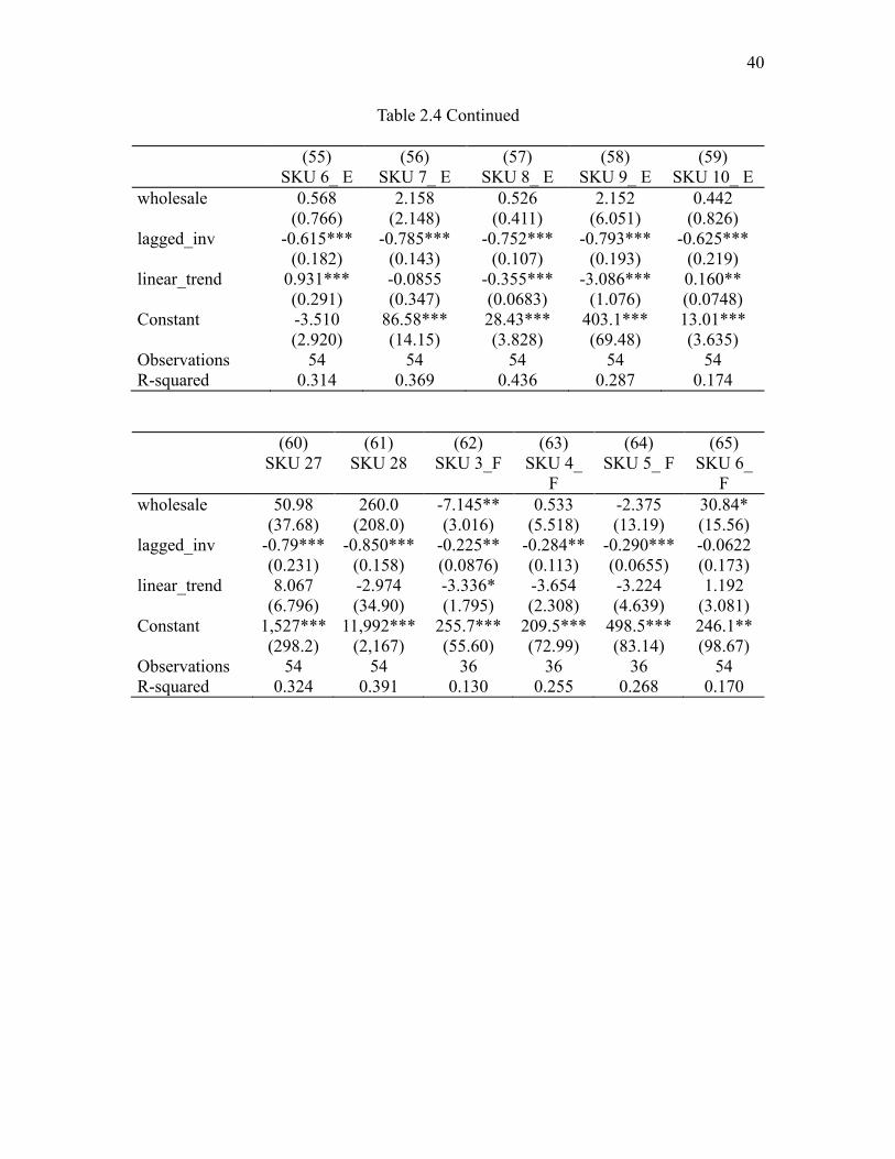
40
Table 2.4 Continued
(55) (56) (57) (58) (59)
SKU 6_ E SKU 7_ E SKU 8_ E SKU 9_ E SKU 10_ E
wholesale 0.568 2.158 0.526 2.152 0.442
(0.766) (2.148) (0.411) (6.051) (0.826)
lagged_inv -0.615*** -0.785*** -0.752*** -0.793*** -0.625***
(0.182) (0.143) (0.107) (0.193) (0.219)
linear_trend 0.931*** -0.0855 -0.355*** -3.086*** 0.160**
(0.291) (0.347) (0.0683) (1.076) (0.0748)
Constant -3.510 86.58*** 28.43*** 403.1*** 13.01***
(2.920) (14.15) (3.828) (69.48) (3.635)
Observations 54 54 54 54 54
R-squared 0.314 0.369 0.436 0.287 0.174
(60) (61) (62) (63) (64) (65)
SKU 27 SKU 28 SKU 3_F SKU 4_
F
SKU 5_ F SKU 6_
F
wholesale 50.98 260.0 -7.145** 0.533 -2.375 30.84*
(37.68) (208.0) (3.016) (5.518) (13.19) (15.56)
lagged_inv -0.79*** -0.850*** -0.225** -0.284** -0.290*** -0.0622
(0.231) (0.158) (0.0876) (0.113) (0.0655) (0.173)
linear_trend 8.067 -2.974 -3.336* -3.654 -3.224 1.192
(6.796) (34.90) (1.795) (2.308) (4.639) (3.081)
Constant 1,527*** 11,992*** 255.7*** 209.5*** 498.5*** 246.1**
(298.2) (2,167) (55.60) (72.99) (83.14) (98.67)
Observations 54 54 36 36 36 54
R-squared 0.324 0.391 0.130 0.255 0.268 0.170
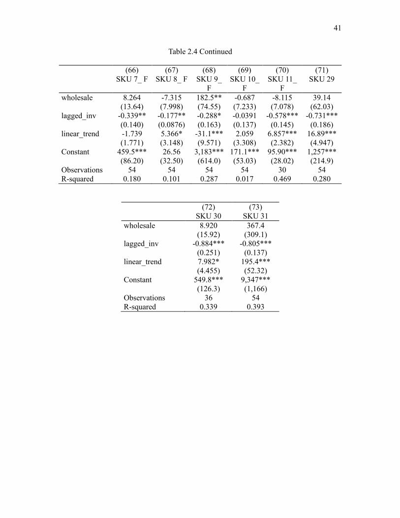
41
Table 2.4 Continued
(66) (67) (68) (69) (70) (71)
SKU 7_ F SKU 8_ F SKU 9_
F
SKU 10_
F
SKU 11_
F
SKU 29
wholesale 8.264 -7.315 182.5** -0.687 -8.115 39.14
(13.64) (7.998) (74.55) (7.233) (7.078) (62.03)
lagged_inv -0.339** -0.177** -0.288* -0.0391 -0.578*** -0.731***
(0.140) (0.0876) (0.163) (0.137) (0.145) (0.186)
linear_trend -1.739 5.366* -31.1*** 2.059 6.857*** 16.89***
(1.771) (3.148) (9.571) (3.308) (2.382) (4.947)
Constant 459.5*** 26.56 3,183*** 171.1*** 95.90*** 1,257***
(86.20) (32.50) (614.0) (53.03) (28.02) (214.9)
Observations 54 54 54 54 30 54
R-squared 0.180 0.101 0.287 0.017 0.469 0.280
(72) (73)
SKU 30 SKU 31
wholesale 8.920 367.4
(15.92) (309.1)
lagged_inv -0.884*** -0.805***
(0.251) (0.137)
linear_trend 7.982* 195.4***
(4.455) (52.32)
Constant 549.8*** 9,347***
(126.3) (1,166)
Observations 36 54
R-squared 0.339 0.393
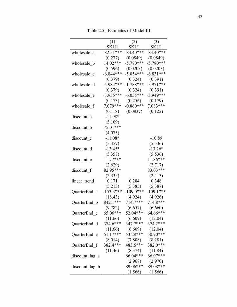
42
Table 2.5: Estimates of Model III
(1) (2) (3)
SKU1 SKU1 SKU1
wholesale_a -82.51*** -83.40*** -83.40***
(0.277) (0.0849) (0.0849)
wholesale_b 14.02*** -5.780*** -5.780***
(0.596) (0.0203) (0.0203)
wholesale_c -6.844*** -5.054*** -6.831***
(0.379) (0.324) (0.391)
wholesale_d -5.984*** -1.788*** -5.971***
(0.379) (0.324) (0.391)
wholesale_e -3.955*** -6.055*** -3.949***
(0.173) (0.256) (0.179)
wholesale_f 7.079*** -0.860*** 7.083***
(0.118) (0.0837) (0.122)
discount_a -11.98*
(5.169)
discount_b 75.01***
(4.075)
discount_c -11.08* -10.89
(5.357) (5.536)
discount_d -13.45* -13.26*
(5.357) (5.536)
discount_e 11.77*** 11.86***
(2.629) (2.717)
discount_f 82.95*** 83.03***
(2.335) (2.413)
linear_trend 0.171 0.284 0.348
(5.213) (5.385) (5.387)
QuarterEnd_a -153.3*** -109.0*** -109.1***
(18.43) (4.924) (4.926)
QuarterEnd_b 842.1*** 714.7*** 714.8***
(9.782) (6.657) (6.660)
QuarterEnd_c 65.06*** 52.04*** 64.66***
(11.66) (6.609) (12.04)
QuarterEnd_d 374.6*** 347.7*** 374.2***
(11.66) (6.609) (12.04)
QuarterEnd_e 51.17*** 53.28*** 50.90***
(8.014) (7.808) (8.281)
QuarterEnd_f 382.4*** 483.6*** 382.0***
(11.46) (8.374) (11.84)
discount_lag_a 66.04*** 66.07***
(2.968) (2.970)
discount_lag_b 89.06*** 89.08***
(1.566) (1.566)
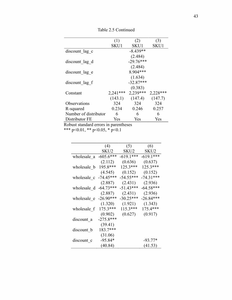
43
Table 2.5 Continued
(1) (2) (3)
SKU1 SKU1 SKU1
discount_lag_c -8.439**
(2.484)
discount_lag_d -29.76***
(2.484)
discount_lag_e 8.904***
(1.634)
discount_lag_f -32.87***
(0.383)
Constant 2,241*** 2,239*** 2,228***
(143.1) (147.4) (147.7)
Observations 324 324 324
R-squared 0.234 0.246 0.257
Number of distributor 6 6 6
Distributor FE Yes Yes Yes
Robust standard errors in parentheses
*** p<0.01, ** p<0.05, * p<0.1
(4) (5) (6)
SKU2 SKU2 SKU2
wholesale_a -605.6*** -619.1*** -619.1***
(2.112) (0.636) (0.637)
wholesale_b 195.8*** 125.3*** 125.3***
(4.545) (0.152) (0.152)
wholesale_c -74.45*** -54.55*** -74.31***
(2.887) (2.431) (2.936)
wholesale_d -64.73*** -51.43*** -64.58***
(2.887) (2.431) (2.936)
wholesale_e -26.90*** -30.25*** -26.84***
(1.320) (1.921) (1.343)
wholesale_f 175.3*** 115.3*** 175.4***
(0.902) (0.627) (0.917)
discount_a -275.8***
(39.41)
discount_b 183.7***
(31.06)
discount_c -95.84* -93.77*
(40.84) (41.53)
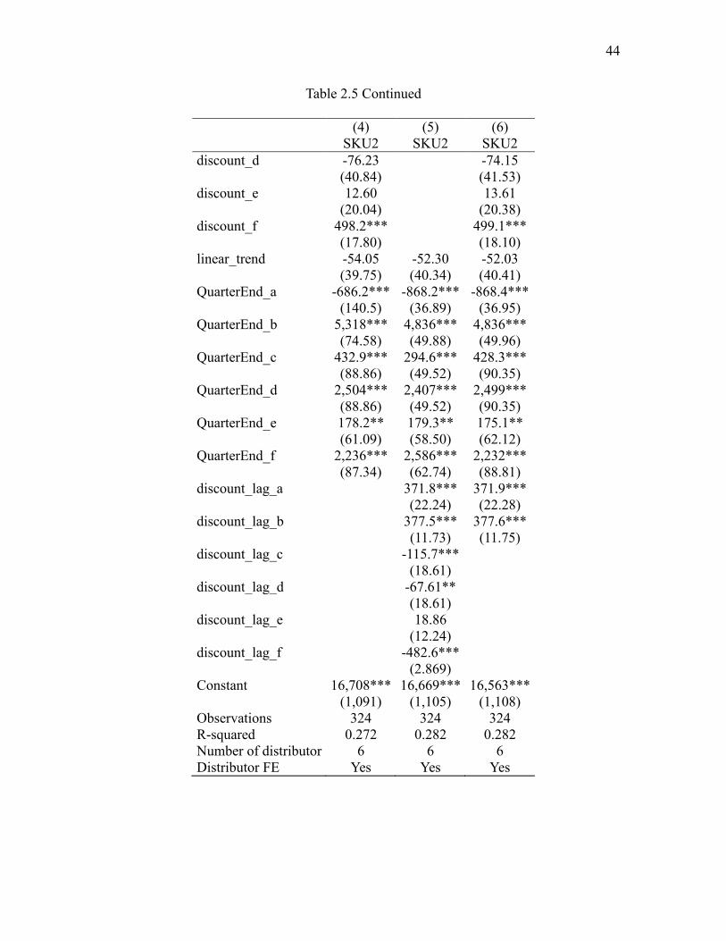
44
Table 2.5 Continued
(4) (5) (6)
SKU2 SKU2 SKU2
discount_d -76.23 -74.15
(40.84) (41.53)
discount_e 12.60 13.61
(20.04) (20.38)
discount_f 498.2*** 499.1***
(17.80) (18.10)
linear_trend -54.05 -52.30 -52.03
(39.75) (40.34) (40.41)
QuarterEnd_a -686.2*** -868.2*** -868.4***
(140.5) (36.89) (36.95)
QuarterEnd_b 5,318*** 4,836*** 4,836***
(74.58) (49.88) (49.96)
QuarterEnd_c 432.9*** 294.6*** 428.3***
(88.86) (49.52) (90.35)
QuarterEnd_d 2,504*** 2,407*** 2,499***
(88.86) (49.52) (90.35)
QuarterEnd_e 178.2** 179.3** 175.1**
(61.09) (58.50) (62.12)
QuarterEnd_f 2,236*** 2,586*** 2,232***
(87.34) (62.74) (88.81)
discount_lag_a 371.8*** 371.9***
(22.24) (22.28)
discount_lag_b 377.5*** 377.6***
(11.73) (11.75)
discount_lag_c -115.7***
(18.61)
discount_lag_d -67.61**
(18.61)
discount_lag_e 18.86
(12.24)
discount_lag_f -482.6***
(2.869)
Constant 16,708*** 16,669*** 16,563***
(1,091) (1,105) (1,108)
Observations 324 324 324
R-squared 0.272 0.282 0.282
Number of distributor 6 6 6
Distributor FE Yes Yes Yes
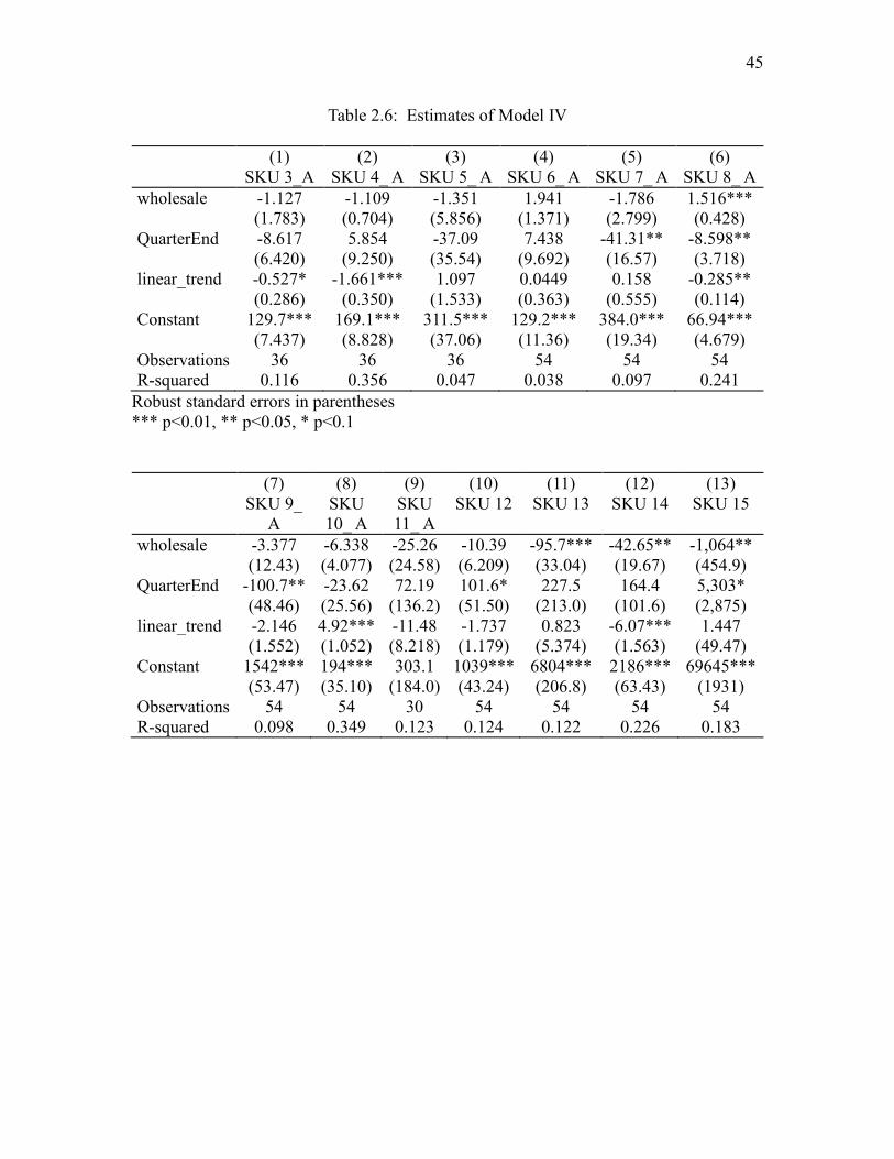
45
Table 2.6: Estimates of Model IV
(1) (2) (3) (4) (5) (6)
SKU 3_A SKU 4_ A SKU 5_ A SKU 6_ A SKU 7_ A SKU 8_ A
wholesale -1.127 -1.109 -1.351 1.941 -1.786 1.516***
(1.783) (0.704) (5.856) (1.371) (2.799) (0.428)
QuarterEnd -8.617 5.854 -37.09 7.438 -41.31** -8.598**
(6.420) (9.250) (35.54) (9.692) (16.57) (3.718)
linear_trend -0.527* -1.661*** 1.097 0.0449 0.158 -0.285**
(0.286) (0.350) (1.533) (0.363) (0.555) (0.114)
Constant 129.7*** 169.1*** 311.5*** 129.2*** 384.0*** 66.94***
(7.437) (8.828) (37.06) (11.36) (19.34) (4.679)
Observations 36 36 36 54 54 54
R-squared 0.116 0.356 0.047 0.038 0.097 0.241
Robust standard errors in parentheses
*** p<0.01, ** p<0.05, * p<0.1
(7) (8) (9) (10) (11) (12) (13)
SKU 9_
A
SKU
10_ A
SKU
11_ A
SKU 12 SKU 13 SKU 14 SKU 15
wholesale -3.377 -6.338 -25.26 -10.39 -95.7*** -42.65** -1,064**
(12.43) (4.077) (24.58) (6.209) (33.04) (19.67) (454.9)
QuarterEnd -100.7** -23.62 72.19 101.6* 227.5 164.4 5,303*
(48.46) (25.56) (136.2) (51.50) (213.0) (101.6) (2,875)
linear_trend -2.146 4.92*** -11.48 -1.737 0.823 -6.07*** 1.447
(1.552) (1.052) (8.218) (1.179) (5.374) (1.563) (49.47)
Constant 1542*** 194*** 303.1 1039*** 6804*** 2186*** 69645***
(53.47) (35.10) (184.0) (43.24) (206.8) (63.43) (1931)
Observations 54 54 30 54 54 54 54
R-squared 0.098 0.349 0.123 0.124 0.122 0.226 0.183
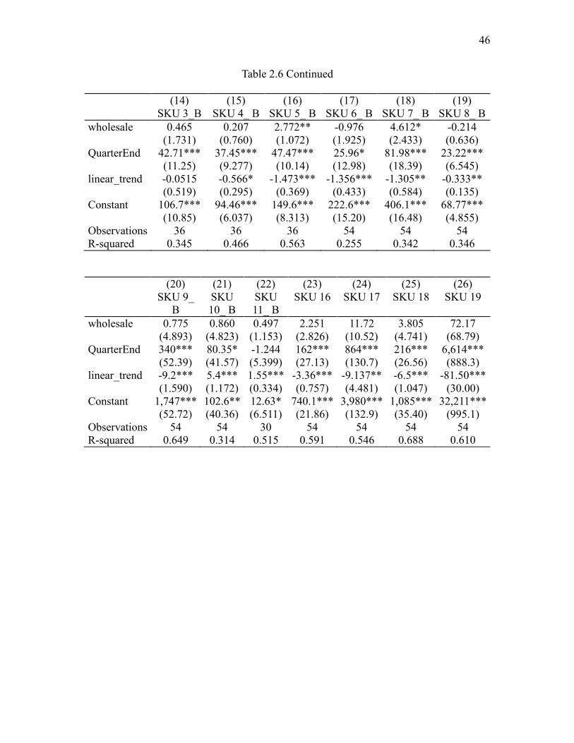
46
Table 2.6 Continued
(14) (15) (16) (17) (18) (19)
SKU 3_B SKU 4_ B SKU 5_ B SKU 6_ B SKU 7_ B SKU 8_ B
wholesale 0.465 0.207 2.772** -0.976 4.612* -0.214
(1.731) (0.760) (1.072) (1.925) (2.433) (0.636)
QuarterEnd 42.71*** 37.45*** 47.47*** 25.96* 81.98*** 23.22***
(11.25) (9.277) (10.14) (12.98) (18.39) (6.545)
linear_trend -0.0515 -0.566* -1.473*** -1.356*** -1.305** -0.333**
(0.519) (0.295) (0.369) (0.433) (0.584) (0.135)
Constant 106.7*** 94.46*** 149.6*** 222.6*** 406.1*** 68.77***
(10.85) (6.037) (8.313) (15.20) (16.48) (4.855)
Observations 36 36 36 54 54 54
R-squared 0.345 0.466 0.563 0.255 0.342 0.346
(20) (21) (22) (23) (24) (25) (26)
SKU 9_
B
SKU
10_ B
SKU
11_ B
SKU 16 SKU 17 SKU 18 SKU 19
wholesale 0.775 0.860 0.497 2.251 11.72 3.805 72.17
(4.893) (4.823) (1.153) (2.826) (10.52) (4.741) (68.79)
QuarterEnd 340*** 80.35* -1.244 162*** 864*** 216*** 6,614***
(52.39) (41.57) (5.399) (27.13) (130.7) (26.56) (888.3)
linear_trend -9.2*** 5.4*** 1.55*** -3.36*** -9.137** -6.5*** -81.50***
(1.590) (1.172) (0.334) (0.757) (4.481) (1.047) (30.00)
Constant 1,747*** 102.6** 12.63* 740.1*** 3,980*** 1,085*** 32,211***
(52.72) (40.36) (6.511) (21.86) (132.9) (35.40) (995.1)
Observations 54 54 30 54 54 54 54
R-squared 0.649 0.314 0.515 0.591 0.546 0.688 0.610
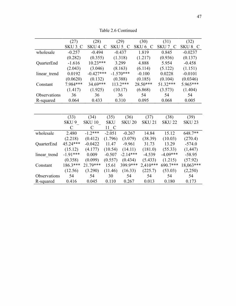
47
Table 2.6 Continued
(27) (28) (29) (30) (31) (32)
SKU 3_C SKU 4_ C SKU 5_ C SKU 6_ C SKU 7_ C SKU 8_ C
wholesale -0.257 -0.494 -0.437 1.819 0.845 -0.0237
(0.282) (0.355) (1.318) (1.217) (0.936) (0.137)
QuarterEnd -1.616 10.23*** 3.299 4.888 5.954 -0.458
(2.043) (3.046) (8.163) (6.114) (5.122) (1.151)
linear_trend 0.0192 -0.427*** -1.570*** -0.100 0.0228 -0.0101
(0.0620) (0.132) (0.388) (0.185) (0.104) (0.0346)
Constant 7.984*** 34.69*** 113.2*** 28.50*** 51.32*** 5.965***
(1.417) (1.925) (10.17) (6.868) (3.573) (1.404)
Observations 36 36 36 54 54 54
R-squared 0.064 0.433 0.310 0.095 0.068 0.005
(33) (34) (35) (36) (37) (38) (39)
SKU 9_
C
SKU 10_
C
SKU
11_ C
SKU 20 SKU 21 SKU 22 SKU 23
wholesale 2.480 -1.2*** -2.051 -0.267 14.84 15.12 648.7**
(2.218) (0.412) (1.796) (3.079) (38.39) (10.03) (270.4)
QuarterEnd 45.24*** -0.0422 11.47 -9.961 31.73 13.29 -574.0
(15.12) (4.177) (10.54) (14.11) (181.0) (55.33) (1,447)
linear_trend -1.91*** 0.009 -0.507 -2.14*** -4.539 -4.09*** -58.95
(0.358) (0.099) (0.557) (0.434) (5.433) (1.215) (57.92)
Constant 186.3*** 21.79*** 15.61 399.9*** 2,410*** 690.7*** 18,063***
(12.56) (3.290) (11.46) (16.33) (225.7) (53.03) (2,250)
Observations 54 54 30 54 54 54 54
R-squared 0.416 0.045 0.110 0.267 0.013 0.180 0.173
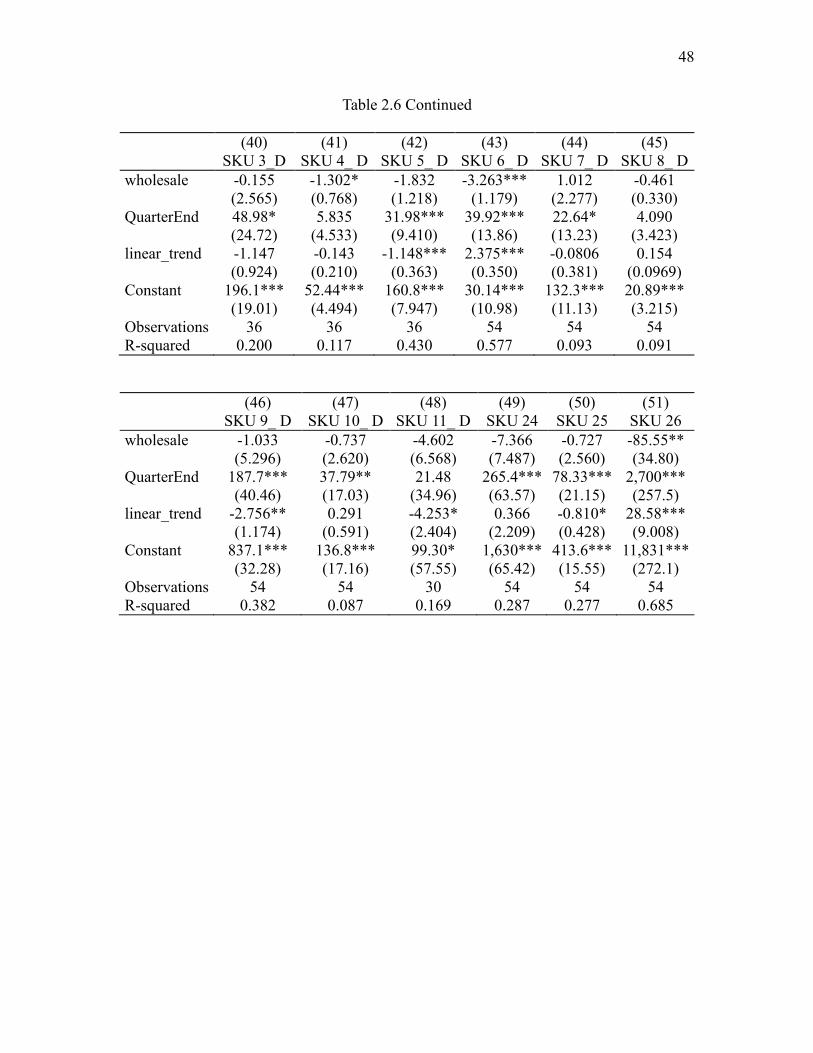
48
Table 2.6 Continued
(40) (41) (42) (43) (44) (45)
SKU 3_D SKU 4_ D SKU 5_ D SKU 6_ D SKU 7_ D SKU 8_ D
wholesale -0.155 -1.302* -1.832 -3.263*** 1.012 -0.461
(2.565) (0.768) (1.218) (1.179) (2.277) (0.330)
QuarterEnd 48.98* 5.835 31.98*** 39.92*** 22.64* 4.090
(24.72) (4.533) (9.410) (13.86) (13.23) (3.423)
linear_trend -1.147 -0.143 -1.148*** 2.375*** -0.0806 0.154
(0.924) (0.210) (0.363) (0.350) (0.381) (0.0969)
Constant 196.1*** 52.44*** 160.8*** 30.14*** 132.3*** 20.89***
(19.01) (4.494) (7.947) (10.98) (11.13) (3.215)
Observations 36 36 36 54 54 54
R-squared 0.200 0.117 0.430 0.577 0.093 0.091
(46) (47) (48) (49) (50) (51)
SKU 9_ D SKU 10_ D SKU 11_ D SKU 24 SKU 25 SKU 26
wholesale -1.033 -0.737 -4.602 -7.366 -0.727 -85.55**
(5.296) (2.620) (6.568) (7.487) (2.560) (34.80)
QuarterEnd 187.7*** 37.79** 21.48 265.4*** 78.33*** 2,700***
(40.46) (17.03) (34.96) (63.57) (21.15) (257.5)
linear_trend -2.756** 0.291 -4.253* 0.366 -0.810* 28.58***
(1.174) (0.591) (2.404) (2.209) (0.428) (9.008)
Constant 837.1*** 136.8*** 99.30* 1,630*** 413.6*** 11,831***
(32.28) (17.16) (57.55) (65.42) (15.55) (272.1)
Observations 54 54 30 54 54 54
R-squared 0.382 0.087 0.169 0.287 0.277 0.685
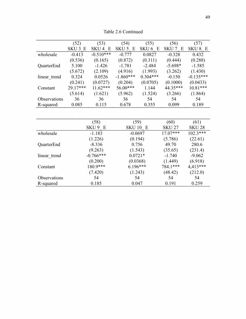
49
Table 2.6 Continued
(52) (53) (54) (55) (56) (57)
SKU 3_E SKU 4_ E SKU 5_ E SKU 6_ E SKU 7_ E SKU 8_ E
wholesale -0.413 -0.510*** -0.777 0.0827 -0.328 0.432
(0.536) (0.165) (0.872) (0.311) (0.444) (0.288)
QuarterEnd 5.100 -1.426 -1.781 -2.484 -5.698* -1.585
(5.672) (2.109) (4.916) (1.993) (3.262) (1.430)
linear_trend 0.324 0.0526 -1.860*** 0.304*** -0.150 -0.135***
(0.241) (0.0727) (0.204) (0.0705) (0.1000) (0.0433)
Constant 29.17*** 11.62*** 56.00*** 1.144 44.35*** 10.81***
(5.614) (1.621) (5.962) (1.524) (3.266) (1.864)
Observations 36 36 36 54 54 54
R-squared 0.085 0.115 0.678 0.355 0.099 0.189
(58) (59) (60) (61)
SKU 9_ E SKU 10_ E SKU 27 SKU 28
wholesale -1.183 -0.0697 17.07*** 102.3***
(1.226) (0.194) (5.786) (22.61)
QuarterEnd -8.336 0.756 49.70 280.6
(9.263) (1.543) (35.65) (231.4)
linear_trend -0.766*** 0.0721* -1.740 -9.062
(0.200) (0.0368) (1.449) (6.918)
Constant 180.9*** 6.196*** 784.1*** 4,413***
(7.420) (1.243) (48.42) (212.0)
Observations 54 54 54 54
R-squared 0.185 0.047 0.191 0.259
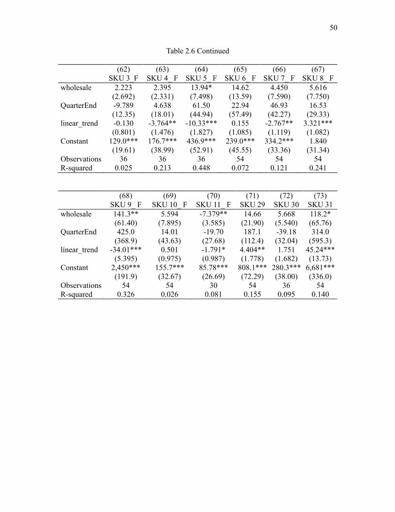
50
Table 2.6 Continued
(62) (63) (64) (65) (66) (67)
SKU 3_F SKU 4_ F SKU 5_ F SKU 6_ F SKU 7_ F SKU 8_ F
wholesale 2.223 2.395 13.94* 14.62 4.450 5.616
(2.692) (2.331) (7.498) (13.59) (7.590) (7.750)
QuarterEnd -9.789 4.638 61.50 22.94 46.93 16.53
(12.35) (18.01) (44.94) (57.49) (42.27) (29.33)
linear_trend -0.130 -3.764** -10.33*** 0.155 -2.767** 3.321***
(0.801) (1.476) (1.827) (1.085) (1.119) (1.082)
Constant 129.0*** 176.7*** 436.9*** 239.0*** 334.2*** 1.840
(19.61) (38.99) (52.91) (45.55) (33.36) (31.34)
Observations 36 36 36 54 54 54
R-squared 0.025 0.213 0.448 0.072 0.121 0.241
(68) (69) (70) (71) (72) (73)
SKU 9_ F SKU 10_ F SKU 11_ F SKU 29 SKU 30 SKU 31
wholesale 141.3** 5.594 -7.379** 14.66 5.668 118.2*
(61.40) (7.895) (3.585) (21.90) (5.540) (65.76)
QuarterEnd 425.0 14.01 -19.70 187.1 -39.18 314.0
(368.9) (43.63) (27.68) (112.4) (32.04) (595.3)
linear_trend -34.01*** 0.501 -1.791* 4.404** 1.751 45.24***
(5.395) (0.975) (0.987) (1.778) (1.682) (13.73)
Constant 2,450*** 155.7*** 85.78*** 808.1*** 280.3*** 6,681***
(191.9) (32.67) (26.69) (72.29) (38.00) (336.0)
Observations 54 54 30 54 36 54
R-squared 0.326 0.026 0.081 0.155 0.095 0.140
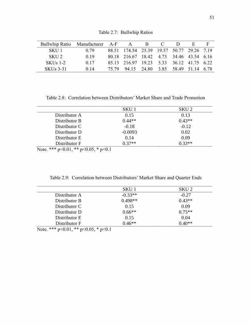
51
Table 2.7: Bullwhip Ratios
Bullwhip Ratio Manufacturer A-F A B C D E F
SKU 1 0.79 88.51 174.54 25.39 19.57 50.77 29.26 7.19
SKU 2 0.19 80.18 216.67 18.42 4.73 34.46 43.54 6.16
SKUs 1-2 0.17 85.13 216.97 19.23 5.33 36.12 41.75 6.22
SKUs 3-31 0.14 75.79 94.15 24.80 3.85 58.49 51.14 6.78
Table 2.8: Correlation between Distributors’ Market Share and Trade Promotion
SKU 1 SKU 2
Distributor A 0.15 0.13
Distributor B 0.44** 0.43**
Distributor C -0.18 -0.12
Distributor D -0.0093 0.02
Distributor E 0.14 0.09
Distributor F 0.37** 0.33**
Note. *** p<0.01, ** p<0.05, * p<0.1
Table 2.9: Correlation between Distributors’ Market Share and Quarter Ends
SKU 1 SKU 2
Distributor A -0.33** -0.27
Distributor B 0.498** 0.43**
Distributor C 0.15 0.09
Distributor D 0.66** 0.75**
Distributor E 0.15 0.04
Distributor F 0.46** 0.40**
Note. *** p<0.01, ** p<0.05, * p<0.1
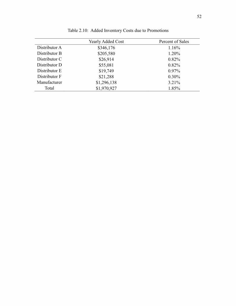
52
Table 2.10: Added Inventory Costs due to Promotions
Yearly Added Cost Percent of Sales
Distributor A $346,176 1.16%
Distributor B $205,580 1.20%
Distributor C $26,914 0.82%
Distributor D $55,081 0.82%
Distributor E $19,749 0.97%
Distributor F $21,288 0.30%
Manufacturer $1,296,138 3.21%
Total $1,970,927 1.85%
CHAPTER 3
IN SEARCH OF INTRA-ECHELON BULLWHIPS
3.1 Introduction
Supply chain managers and operations researchers alike have invested considerable
effort over the past several decades to better understand the bullwhip effect and mitigate
its negative consequences. The seminal paper of Lee et al. (1997a) defines the bullwhip
effect as “the phenomenon where orders to the supplier tend to have larger variance than
sales to the buyer (i.e., orders distortion), and the distortion propagates upstream in an
amplified form (i.e., variance amplification)” (p. 546). Researchers have explored the cause
of the bullwhip phenomenon and proposed a variety of remedies (e.g., Lee et al., 1997a;
Chen et al., 2000; Chen & Lee, 2012). Other researchers have focused on empirically
measuring the level of the bullwhip in practice and testing for possible drivers of its
magnitude (e.g., Bray & Mendelson, 2012; Cachon et al., 2007; Dooley et al., 2010; Duan
et al., 2015; Fransoo & Wouter, 2000; Lai, 2005; Jin et al., 2015; Mackelprang & Malhotra,
2015; Shan et al., 2014; Zotteri, 2013).
The bullwhip definition noted above effectively looks across the firm, comparing
the variability in the firm’s orders it places with its suppliers to the variability in the orders
the firm receives from its customers. If the measure is greater than one then the bullwhip
effect is said to exist, while if it is less than one then an antibullwhip exists. That is, the

54
firm smooths rather than amplifies its order variability. This conventional bullwhip
measure views the firm as one “entity” in the supply chain and constitutes an inter-firm
bullwhip measure.
While the conventional bullwhip measure is informative and useful for determining
what happens across a firm in the supply chain, numerous actions inside the firm contribute
to its conventional bullwhip measure. By decomposing the firm’s conventional inter-firm
bullwhip measure into three intra-firm (component) bullwhips, we offer the firm a simple
and readily-implementable framework to employ “in search of” its internal bullwhip, and
to track and reduce the variability in its product flow streams.
The first bullwhip component in our framework is what we call the shipment
bullwhip – it describes the variability in the firm’s shipment (i.e., sales) stream relative to
the stream of demand (i.e., orders received). Moving upstream within the firm, the second
component is referred to as the manufacturing bullwhip – it measures the variability in the
firm’s manufacturing stream relative to its shipment stream. Next is the order bullwhip,
defined as the variability in the stream of orders the firm places relative to the firm’s
manufacturing stream. Mathematically, we show that multiplying these three intra-firm
bullwhips results in the conventional inter-firm bullwhip measure. That is, the conventional
bullwhip measure is the product of the firm’s shipment, manufacturing, and order
bullwhips.
In the remainder of this chapter, inter-firm bullwhip and intra-firm bullwhip are
referred to as inter-echelon bullwhip and intra-echelon bullwhip, respectively, to account
for the possibility that some entity other than a firm (e.g., a division within a firm, an
individual facility within a division, and an industry) is under investigation.
55
Using monthly, industry-level U.S. Census Bureau data, we proceed “in search of”
the magnitude of each of intra-echelon bullwhips across industries, and we examine
correlations between them. For example, we find that in some industries there is a very
strong shipment antibullwhip (the shipment bullwhip measure is well below one, meaning
shipments are much smoother than demands), while in other industries there is a significant
shipment bullwhip (shipments are substantively more variable than demands). While our
data are neither extensive nor informative enough to definitively assign cause and effect,
we are able to make several observations regarding the differences in the industry
characteristics. In general, we find that in industries where there is an antibullwhip in
shipping, there is bullwhip created in manufacturing and/or ordering. However, industries
that exhibit an antibullwhip in manufacturing also tend to order in a smoother stream than
they manufacture (i.e., an antibullwhip in ordering). Our work therefore acts as a set of
mini-case studies that can be used to motivate future research into what explains the
observed disparity in intra-echelon bullwhips across industries. Although we report results
based on industry-level data, the same analysis can also be performed at a less aggregate
level (e.g., the divisional level, a product category level, and a product level).
In addition to offering managers a framework for monitoring intra-echelon
bullwhips, we provide insight into the impact of their decisions regarding the bullwhip
measurement time interval. Our results are consistent with Chen and Lee (2012) who
propose that time aggregation tends to dampen the bullwhip (i.e., when the bullwhip ratio
is above one, time aggregation reduces it). Moreover, we find new empirical evidence that
suggests time aggregate tends to amplify the bullwhip ratio when an antibullwhip exists;
time aggregation seems to cause the bullwhip ratio to converge to one. An additional

56
contribution of our work is to demonstrate the importance of properly setting the starting
point for the time aggregation interval. For example, while many retailers use a February
1 quarterly start date, we show that a start date of January 1 may be more appropriate for
the purposes of bullwhip measurement.
In sum, our empirical observations provide additional insight into the factors
managers should take into account when determining their shipment schedules (which
impact their shipment bullwhip), when setting their manufacturing plans (which impact
their manufacturing bullwhip), and when establishing their order quantities (which impact
their order bullwhip). While other researchers have studied some of the internal factors that
might influence the overall bullwhip, such as inventory stocking levels (e.g., Svensson,
2003) and manufacturing activities (e.g., Taylor, 1999), we contribute to this body of work
by demonstrating how the intra-echelon bullwhips contribute to the overall inter-echelon
bullwhip, both analytically and empirically.
The chapter proceeds as follows. In section 3.2 we explicitly lay out the bullwhip
decomposition, showing how the shipment, manufacturing, and order bullwhips contribute
to the overall (conventional) bullwhip measure. Next, in section 3.3 we develop hypotheses
regarding whether we expect an intra-echelon bullwhip to be greater than or less than one
(i.e., whether the bullwhip or antibullwhip predominates). We also hypothesize as to the
effect of time aggregation and interval starting point. We describe our dataset in section
3.4, proceed to test our hypotheses in section 3.5, and summarize the results in section 3.6.
57
3.2 Bullwhip Decomposition
An ideal supply chain might be described as having a smooth flow of inventory
throughout the chain. Every echelon would 1) receive a perfectly smooth demand stream
from its downstream customers; 2) fulfill this demand stream with a perfectly-matched
shipment (i.e., sales) stream; 3) manufacture in a smooth just-in-time fashion, shipping
immediately on completion with no need for any finished goods inventory; 4) order raw
materials (RM) from upstream suppliers at a smooth rate that exactly matches the
manufacturing flow stream; and 5) receive raw materials (i.e., fulfillment of orders) from
its supplier in just-in-time fashion so as to avoid the need for raw materials inventory. This
would result in no variance in any flow stream anywhere in the supply chain, that is, no
bullwhip (or smoothing). Note that in this description the upstream progression could be
executed via a pull system – downstream demand pulls shipments, shipments pull
manufacturing, and manufacturing pulls orders as one moves upstream in the supply chain.
Compared to this ideal, actual supply chains differ substantially, namely, there is
virtually always some level of variability in each of the flow streams identified above. The
framework we introduce in this chapter, as depicted in Figure 3.1, characterizes how the
variability in each of these flow streams is either amplified or dampened when pulling the
upstream flow. Note that our framework does not hinge on the use of a pull system. Instead,
we use this terminology simply for convenience.
Starting at the upper left of Figure 3.1, an echelon at any point in the supply chain
(which we refer to as the focal echelon) receives a demand stream that has variance denoted
by 𝑉𝐷𝐹 (the superscript F refers to the focal echelon, while the subscript D denotes that this
parameter is the variance in the demand stream). Echelon F may choose not to (or may not

58
be able to) fulfill demands immediately, so its shipment stream may not exactly match its
demand stream (by “demand stream” we mean the stream of orders received). For example,
the economy may suddenly get stronger, creating a surge in demand that echelon F cannot
immediately fill via manufacturing output and/or inventory. Thus, the variance in echelon
F’s shipment stream, which we denote by 𝑉𝑆𝐹 (the superscript again denoting echelon F
and the subscript S referring to the shipment stream), may differ from the variance in its
demand stream, 𝑉𝐷𝐹. We define the variance ratio
𝑉𝑆𝐹
𝑉𝐷𝐹 to be the echelon’s shipment bullwhip,
and denote this bullwhip ratio by 𝐵𝑆𝐹. Note that the shipment bullwhip might indicate an
amplification of the demand stream (𝐵𝑆𝐹 =
𝑉𝑆𝐹
𝑉𝐷𝐹 > 1) or a smoothing (𝐵𝑆
𝐹 < 1).
If echelon F holds finished goods (FG) inventory at any point in time, then its
manufacturing output stream will not necessarily match its shipment stream. For example,
demand may be seasonal, and even if demand is fully known in advance, echelon F may
find it optimal to smooth its output (overproduce and build up finished goods inventory in
periods of slack demand and under-produce and ship from inventory in periods of high
demand). If demand is uncertain, this further complicates echelon F’s decision making with
regard to the manufacturing stream. The manufacturing stream may become even further
disconnected from the shipment stream due to factors such as the desirability of batch
manufacturing. In other words, there may be what we denote as a manufacturing bullwhip
within the echelon, defined as 𝐵𝑀𝐹 =
𝑉𝑀𝐹
𝑉𝑆𝐹 , where 𝑉𝑀
𝐹 denotes the variance in the
manufacturing stream. The manufacturing bullwhip recognizes the fact that the
manufacturing stream may differ from the shipment stream. Again, the manufacturing
bullwhip may indicate an amplification (𝐵𝑀𝐹 > 1) or smoothing (𝐵𝑀
𝐹 < 1).

59
Similarly, it may not be optimal for echelon F to order raw materials to exactly
follow its manufacturing stream (i.e., for its order stream to follow its manufacturing
stream). For example, an upstream echelon’s supply may be uncertain or it may offer end-
of-quarter discounts or have other promotions due to goods surpluses. Factors such as these
may make it optimal for echelon F to alter its order stream as compared to the
manufacturing stream (i.e., it may be optimal for an echelon to plan to hold raw materials
inventory). We denote the variance in stream of orders that echelon F places by 𝑉𝑂𝐹, and
define the order bullwhip as 𝐵𝑂𝐹 =
𝑉𝑂𝐹
𝑉𝑀𝐹, where 𝑉𝑂
𝐹 denotes the variance in the order stream.
Similar to the above discussion, the order bullwhip may indicate an amplification (𝐵𝑂𝐹 > 1)
or a smoothing (𝐵𝑂𝐹 < 1).
As previously noted, Lee et al. (1997a) effectively define the bullwhip as “order
distortion.” Accordingly, echelon F’s overall, or “undecomposed,” bullwhip ratio (which
we will denote by 𝐵𝐹 ) is defined to be the variance in the orders echelon F places with its
suppliers (𝑉𝑂𝐹 ) divided by the variance in the orders received by echelon F from its
customers (𝑉𝐷𝐹). That is:
𝐵𝐹 =𝑉𝑂
𝐹
𝑉𝐷𝐹 = (
𝑉𝑆𝐹
𝑉𝐷𝐹) (
𝑉𝑀𝐹
𝑉𝑆𝐹) (
𝑉𝑂𝐹
𝑉𝑀𝐹) = 𝐵𝑆
𝐹 𝐵𝑀𝐹 𝐵𝑂
𝐹 (3.1)
Hereafter, when we use “bullwhip” as a stand-alone term, it will be used to mean
the undecomposed bullwhip 𝐵𝐹 , or its surrogate (see discussion on a surrogate bullwhip
measure below). Note that equation (3.1) decomposes echelon F’s inter-echelon bullwhip
into three intra-echelon bullwhips. Starting from the downstream demand side of the
echelon, the three intra-echelon bullwhips are the shipment bullwhip (variability in
shipment flows as compared to demand), the manufacturing bullwhip (variability in

60
manufacturing flows as compared to shipments), and the order bullwhip (variability in the
flow of orders placed as compared to manufacturing flows). The same setup applies for
echelon F’s supplier, one level upstream in the supply chain. Using a superscript of U to
denote F’s upstream supplier, we have, analogous to equation (3.1), 𝐵𝑈 =𝑉𝑂
𝑈
𝑉𝐷𝑈 =
(𝑉𝑆
𝑈
𝑉𝐷𝑈) (
𝑉𝑀𝑈
𝑉𝑆𝑈) (
𝑉𝑂𝑈
𝑉𝑀𝑈) = 𝐵𝑆
𝑈 𝐵𝑀𝑈 𝐵𝑂
𝑈.
In some previous studies, surrogate measures have been used to estimate the
bullwhip, 𝐵𝐹 . Since we also use these surrogate measures in a subset of our analysis, we
describe these measures here. Specifically, because the dataset used by Cachon et al. (2007)
does not include information for orders placed, they are unable to directly measure 𝑉𝑂𝐹.
Instead, Cachon et al. (2007) calculate what they call “production,” computed as the sales
(i.e., shipments) plus the change in inventory. This production measure effectively
represents the inflow of materials. We use the term “inflow” to reflect the quantity
represented by shipments plus change in inventory, and denote the inflow variance by 𝑉𝐼𝐹
and the inflow bullwhip by 𝐵𝐼𝐹 =
𝑉𝐼𝐹
𝑉𝑂𝐹. Note that we have already effectively defined the
inflow bullwhip (it is not yet another bullwhip) because the inflows to the focal echelon
are effectively equal to the shipments of the upstream supply chain echelon. That is, 𝑉𝐼𝐹 =
𝑉𝑆𝑈, as shown in Figure 3.1. Also note from Figure 3.1 that orders placed by the focal
echelon are effectively the demand (orders received) for the upstream echelon, so 𝑉𝑂𝐹 =
𝑉𝐷𝑈. Thus, 𝐵𝐼
𝐹 = 𝐵𝑆𝑈 =
𝑉𝐼𝐹=𝑉𝑆
𝑈
𝑉𝑂𝐹=𝑉𝐷
𝑈. For some supply chains the Cachon et al. (2007) dataset
includes the orders received so the authors can directly calculate 𝑉𝐷𝐹; in these cases, they
use the measure 𝐵∗𝐹 =
𝑉𝐼𝐹
𝑉𝐷𝐹 as a surrogate for the bullwhip (we put an asterisk in the subscript

61
of the undecomposed bullwhip measure to denote that it is a surrogate measure). Note that
𝐵∗𝐹 =
𝑉𝐼𝐹
𝑉𝐷𝐹 = 𝐵𝑆
𝐹 𝐵𝑀𝐹 𝐵𝑂
𝐹 𝐵𝐼𝐹 = 𝐵𝐹 𝐵𝐼
𝐹 . That is, the bullwhip surrogate 𝐵∗𝐹 is equal to the
conventional bullwhip measure 𝐵𝐹 multiplied by the inflow bullwhip. For other supply
chains their dataset also does not include data for orders received, so they use 𝑉𝑆𝐹 as a
surrogate measure for 𝑉𝐷𝐹 and calculate this (surrogate) bullwhip as 𝐵∗∗
𝐹 =𝑉𝐼
𝐹
𝑉𝑆𝐹 = 𝐵𝑀
𝐹 𝐵𝑂𝐹 𝐵𝐼
𝐹
(the double asterisk is used to denote this particular surrogate bullwhip).
The decomposition of the conventional inter-echelon bullwhip measure 𝐵𝐹 (or its
surrogate) allows us to pinpoint where it is created within the echelon. Specifically, by
looking at its three individual intra-echelon bullwhips, 𝐵𝑆𝐹, 𝐵𝑀
𝐹 , and 𝐵𝑂𝐹, we can identify
whether the amplification (or smoothing) occurs in shipping, and/or manufacturing, and/or
ordering. We next develop hypotheses regarding the direction and magnitude of these
bullwhips and generate hypotheses regarding the time duration over which they should be
measured and the duration starting point.
3.3 Hypothesis Development
We discuss factors plausibly associated with our measures of shipment,
manufacturing, and order bullwhips. In addition to factors discussed below, which all
assume echelon F is making decisions optimally (to maximize expected profit), there may
be behavioral factors which lead to bullwhip amplification (or even possibly smoothing)
(e.g., Bendoly et al., 2006; Croson & Donohue, 2006).
Because of factors such as batch production, production smoothing, and order
batching (Lee et al., 1997a), it is possible that it is not optimal for the bullwhip ratio to

62
equal one (the variance in the stream of orders placed may not be equal to the variance in
the stream of demands). That is, there are a host of factors that may induce echelon F, when
operating optimally, to amplify or dampen a shipment bullwhip, a manufacturing bullwhip,
or an order bullwhip. The decision making becomes even more complex in a multiechelon
supply chain, where one echelon’s decisions impact both the upstream and downstream
echelons. Most likely, identifying the optimal set of decisions given this complexity is not
a tractable problem – and even if the optimal decisions could be identified so as to reduce
costs (or increase revenues) within the supply chain, it will be problematic to determine
how to share the benefit among the various echelons within the chain. However, the
framework discussed herein is intended to help move echelon F one step closer to this
ultimate objective by identifying the importance of tracking intra-echelon bullwhip effects
and adjusting its supply chain based on these observed bullwhips.
3.3.1 Shipment Bullwhip Magnitude
First we examine the shipment bullwhip, defined for echelon F as 𝐵𝑆𝐹 =
𝑉𝑆𝐹
𝑉𝐷𝐹 . There
are several factors suggesting it may not be possible (or desirable) to always ship exactly
per the demand stream. Some dynamics work in the direction of smoothing, and others
work in the direction of variance amplification.
One factor that may (under certain conditions) tend to smooth shipments relative to
demand is an inventory constraint. If inventory holding costs are significant, then it may
not be cost-effective to hold enough inventory to fill all the demand peaks. On the other
hand, the inventory constraint may (under other circumstances) actually work to amplify
shipments relative to demands. Take the case where demands arrive in a relatively smooth
63
pattern, while manufacturing produces in batches. In this case, if inventory is not sufficient
to fill the demand, then shipments will have to wait until a batch of goods is manufactured,
at which point the whole batch (or a significant fraction of it) will be shipped. Thus,
shipments will appear to be “clumpy” when compared to the smooth demand stream.
Analytically, Chen and Lee (2012) show that, under their assumptions, the variance
of sales (shipments, in our terminology) is less than that of demand. The intuition is that
shipments (assumed to be equal to the minimum of demand and on-hand inventory) is a
truncated variable, so inventory censoring makes shipments appear less variable. This
result implies that the shipment bullwhip is less than one. Thus, we propose the following
hypothesis which enables us to test which theory prevails:
HYPOTHESIS 1 (H1). The shipment bullwhip is less than one.
3.3.2 Manufacturing Bullwhip Magnitude
If there are significant fixed costs in manufacturing, or if it is expensive to change
the rate of manufacturing output, then it may be desirable to produce at a constant, steady
pace as compared to following the ups and downs of demand (or more specifically, the ups
and downs of shipments) – the capacity requirement if manufacturing at a smooth output
rate is equal to the average demand rate, while the capacity requirement if following the
peaks and valleys of demand is the highest demand rate. This will tend to smooth
manufacturing relative to shipments, leading to a manufacturing bullwhip of 𝐵𝑀𝐹 =
𝑉𝑀𝐹
𝑉𝑆𝐹 < 1.
On the other hand, echelon F may tend to amplify manufacturing variability as
compared to shipment variability if the firm produces periodically in large batches rather
than manufactures continuously. Echelon F will produce in relatively large batches and

64
then ship from inventory, resulting in relatively more smooth shipments as compared to
manufacturing.
We hypothesize that the forces behind manufacturing smoothing predominate,
given the extensive work in this area by economists (e.g., Fair, 1989; Blinder & Maccini,
1991; Ramey & West, 1999) and the analytical and empirical work of operations
management researchers (e.g., Klein, 1961; Cachon et al., 2007; Bray & Mendelson, 2015).
HYPOTHESIS 2 (H2). The manufacturing bullwhip is less than one.
3.3.3 Order Bullwhip Magnitude
Echelon F may tend to smooth orders relative to manufacturing output in an attempt
to smooth deliveries of raw materials (e.g., it may have docking or “port” capacity
constraints). In addition, it may face pressure from suppliers to buy in a steady stream, to
facilitate lean operations practices, for example. This would lead to order smoothing, with
𝐵𝑂𝐹 =
𝑉𝑂𝐹
𝑉𝑀𝐹 < 1.
However, it is plausible that other factors may influence the variability of orders
relative to that of manufacturing output. For example, the supplier may insist on a
minimum order quantity which exceeds the quantity echelon F might otherwise purchase.
Also, order batching can be a routine part of echelon F’s purchase decision process due to
economies of scale in purchasing associated with factors such as volume discounts and
transportation (e.g., truckload shipments). An upstream echelon may offer periodic or
sporadic price promotions to increase sales volume (shipments) and liquidate excess
inventory, which encourage bulk purchases. The previous literature has reported that
temporary price promotions can lead to forward buys and holding of raw materials
65
inventory (e.g., Blattberg & Levin, 1987; Jin et al., 2015b). Given that both order batching
and price promotions imply that the order stream is more volatile than the manufacturing
stream, we offer the following hypothesis:
HYPOTHESIS 3 (H3). The order bullwhip is greater than one.
3.3.4 Impact of Duration of the Time Interval on the Bullwhip
When empirically measuring the bullwhip effect, researchers need to determine an
appropriate time interval (e.g., weekly, monthly, or quarterly) over which to aggregate the
flow values which are then used in calculations of the variances of orders, shipments, and
manufacturing output. Previous studies (e.g., Fransoo & Wouters, 2000; Cachon et al.,
2007; Chen & Lee, 2012) suggest that the proper aggregation across time should depend
on the specific problem under investigation. Chen and Lee (2012) develop an analytical
model to show that “aggregating data over relatively long time periods can mask the
bullwhip effect” (p. 772). More specifically, they show that for a first-order autoregressive
moving average (ARMA (1, 1)) demand process, the temporally aggregated bullwhip ratio
will approach one in the limit as the aggregation period increases. Furthermore, they show
that if the bullwhip ratio is greater than one, then the ratio will decrease monotonically to
one as the aggregated time period increases. These results suggest that measuring the
variance ratio over a longer time period tends to attenuate the bullwhip (or antibullwhip)
effect, leading to the following hypothesis.
HYPOTHESIS 4 (H4). If the bullwhip ratio is greater than one then time
aggregation decreases the ratio, while if it is less than one then time aggregation
increases the ratio.

66
The smoothing that is hypothesized to occur with aggregation over longer time
intervals may be related to seasonality in data series. To illustrate this possibility, consider
the monthly sales data shown in Figure 3.2 – this plot is representative of sales data across
45 Wal-Mart stores for the period February 2010 to October 2012 (Kaggle, 2015). Note the
seasonality in the data; longer time aggregation intervals have the potential to combine a
maximal demand with a lesser demand (or a minimal demand with a greater demand),
thereby reducing the variance. Assuming the seasonality propagates upstream, the variance
of the upstream flow stream is also diminished, so the impact of seasonality on the bullwhip
will depend on which flow (upstream or downstream) exhibits the most seasonality.
HYPOTHESIS 5 (H5). Seasonality will result in a higher (lower) aggregated
bullwhip ratio when the upstream flow is less (more) seasonal than the downstream
flow.
3.3.5 Impact of the Starting Point of the Time Interval on the Bullwhip
Managers must not only choose the duration of the time interval over which they
measure their bullwhips, they must also set the starting point of that interval. Assume for
the moment that echelon F decides it is most appropriate to use quarterly time durations to
measure and track its bullwhip. Does it matter whether they start the quarter at January 1
versus February 1 versus March 1? (These three start dates effectively cover all possibilities
since we do not consider starting mid-month.)
For all 45 Wal-Mart stores referenced in the Kaggle (2015) dataset, we find that the
variance in the quarterly sales series when starting the quarter in February is less than that
with a January start (see Figure 3.2 for sales at a typical store). This stems from the

67
observation that December is the highest sales month, while January is the lowest sales
month. Grouping the peak and valley into the same quarter partially balances the difference.
Since the variance of sales is the denominator of the bullwhip ratio 𝐵∗∗𝐹 , quarterly
aggregation based on a start in February (Nov/Dec/Jan quarter) or March (Dec/Jan/Feb
quarter) might be expected to result in a higher bullwhip ratio as compared to a start in
January (Oct/Nov/Dec quarter).
Furthermore, a review of quarterly reports from Wal-Mart, Costco, Target, and
Kohl’s suggests that inflows (which in this case roughly equates to receipt of the goods to
be sold) typically lead sales by one quarter – knowing that sales will peak in quarter four
(knowing the seasonality pattern), these retailers prepare by over-producing (i.e., by
increasing inflows) in the third quarter. Assuming inflows (or manufacturing, in the case
of a manufacturer) leads sales (shipments) by one month, the inflow peak occurs in
November and the trough occurs in December, suggesting that inflows would be smoothest
(have the least variance) with the Nov/Dec/Jan (Feb start) and Oct/Nov/Dec (Jan start)
quarters as compared to the Dec/Jan/Feb (March start) quarters. Since the variance of
inflows is the numerator of the bullwhip ratio 𝐵∗∗𝐹 , quarterly aggregation based on a start in
March (Dec/Jan/Feb quarter) might be expected to result in a higher bullwhip ratio as
compared to a start in January (Oct/Nov/Dec quarter) or February (Nov/Dec/Jan quarter).
Regarding previous empirical analysis in this regard, Bray and Mendelson (2012)
argue that different time aggregation schemes will yield different results for any particular
firm, but do not find a general effect.
HYPOTHESIS 6 (H6). For quarterly data, a February or March starting month
results in a higher bullwhip than a January starting month.
68
3.4 Data
Our analysis uses the same monthly, industry-level U.S. Census Bureau data as used
by Cachon et al. (2007). These data are from January 1992 to February 2006 and cover 8
retail, 21 wholesale, and 86 manufacturing industries (we, as do Cachon et al., 2007,
exclude some Census data to avoid possible duplication – some overlap occurs across the
industries because some data within one industry code may be aggregated into another
industry code). We do not incorporate post-2006 data in our analysis (our data range is
from 1992 to 2006) since Dooley et al. (2010) find that firms responded differently to the
economic recession of 2007-2009. Given that we use industry data, the superscript F will
denote the focal industry.
The Census reports monthly sales (i.e., shipments, in the terminology of this chapter)
and inventories for each industry. The industry’s inflow number in a given month t is
calculated as the shipments in that month plus the change in inventory (that month’s
inventory minus last month’s inventory): 𝐼𝑛𝑓𝑙𝑜𝑤𝑡 = 𝑆ℎ𝑖𝑝𝑚𝑒𝑛𝑡𝑠𝑡 + 𝐼𝑛𝑣𝑡 − 𝐼𝑛𝑣𝑡−1 ,
where 𝐼𝑛𝑣𝑡 denotes the inventory in month 𝑡. This inflow number effectively represents
incoming shipments received from the upstream suppliers, that is, it is the upstream
shipment quantity. From these inflow numbers we calculate the inflow variance, 𝑉𝐼𝐹.
We divide manufacturing industries into three sets of data; A, B, and C (see Table
3.1). The A dataset includes 52 industries (A1 through A52) for which data are available
for both demand and shipments (sales). For these industries we can calculate 𝑉𝐷𝐹 and 𝑉𝑆
𝐹,
and thus 𝐵𝑆𝐹. The B dataset includes 23 industries (B1 through B23) for which there are
shipment data but no demand data. The C dataset includes 11 durable goods manufacturing
industries (C1 through C11) for which, again, there are shipment data but not demand (we
69
separate durable goods from other industries given that results may differ).
The Census does not report orders placed for any industries. Since we have the
demand (but not order placement) numbers for the A dataset, we calculate the surrogate
(nondecomposed) bullwhip as 𝐵∗𝐹 =
𝑉𝐼𝐹
𝑉𝐷𝐹 = 𝐵𝑆
𝐹 𝐵𝑀𝐹 𝐵𝑂
𝐹 𝐵𝐼𝐹. For the B and C datasets, since
we do not have demand or order placement data, we report the surrogate bullwhip
𝐵∗∗𝐹 =
𝑉𝐼𝐹
𝑉𝑆𝐹 = 𝐵𝑀
𝐹 𝐵𝑂𝐹 𝐵𝐹
𝐼 .
The U.S. Census reports materials-and-supplies inventory (we infer this to mean
raw materials, RM), work-in-process inventory (WIP), and finished goods inventory (FG)
for 24 manufacturing industries (10 in the A dataset, 11 in B, and 3 in C). In our tables, we
identify these 24 industries by underscoring the letter-number identifier, for example, A6
Computer and Electronic Products, B1 Apparel, and C11 Wood Products. For each of these
24 industries we infer the manufacturing series from its shipments, WIP, and FG, by
assuming the WIP consists of half-finished product: 𝑀𝑎𝑛𝑢𝑓𝑎𝑐𝑡𝑢𝑟𝑖𝑛𝑔𝑡 = 𝑆ℎ𝑖𝑝𝑚𝑒𝑛𝑡𝑠𝑡 +
(𝐹𝐺𝑡 − 𝐹𝐺𝑡−1) + 0.5(𝑊𝐼𝑃𝑡 − 𝑊𝐼𝑃𝑡−1). Thus, for these 24 “underscored” industries, we
can calculate 𝑉𝑀𝐹, and hence, we can determine the manufacturing bullwhip 𝐵𝑀
𝐹 =𝑉𝑀
𝐹
𝑉𝑆𝐹 .
For the 10 underscored industries included in the A data subset (A6, A16, A21, A22,
A24, A29, A40, A44, A49, and A50), we use U.S. Bureau of Economic Analysis (BEA)
Input-Output data to identify the source and magnitude of the materials consumed by each
industry and then infer the orders. Thus, for these 10 industries, we have the full
decomposition of the bullwhip, 𝐵𝑆𝐹, 𝐵𝑀
𝐹 , and 𝐵𝑂𝐹. While this is a relatively limited dataset,
it offers us the unique opportunity to test a number of hypotheses regarding intra-echelon
bullwhips.
70
The demand and shipment series are margin-adjusted to convert into cost dollar
units for inventory valuations. Demand, shipment, and inventory series are price-index-
adjusted so that changes over time are not influenced by inflation. The demand, shipment,
manufacturing, and inflow series are logged and first-differenced to remove the time trend.
(See Cachon et al. (2007) for details regarding, and the rationale behind, these adjustments
to the data.)
The inflow and demand series will probably exhibit some cyclical variation known
as seasonality. We use the seasonality ratio developed by Cachon et al. (2007) to quantify
the seasonality:
𝑆𝑒𝑎𝑠𝑜𝑛𝑎𝑙𝑖𝑡𝑦 𝑅𝑎𝑡𝑖𝑜 =
𝑉[𝐷𝑎𝑡𝑎 𝑆𝑒𝑟𝑖𝑒𝑠] − 𝑉[𝐷𝑒𝑠𝑒𝑎𝑠𝑜𝑛𝑎𝑙𝑖𝑧𝑒𝑑 𝐷𝑎𝑡𝑎 𝑆𝑒𝑟𝑖𝑒𝑠]
𝑉[𝐷𝑎𝑡𝑎 𝑆𝑒𝑟𝑖𝑒𝑠] (3.2)
where the data series can be either the inflow series or the demand series. The
deseasonalized data series is the residuals from regressing data series on 11 monthly
dummy variables. The seasonality ratio represents the fraction of variance that can be
explained by seasonality.
3.5 Results and Discussion
Hypotheses presented in section 3.3.1 through section 3.3.5 are tested in section
3.5.1 through section 3.5.6. These results inform our quests “in search of” intra-echelon
bullwhips. Results also suggest the need for managers to proceed “in search of” their own
internal bullwhips.

71
3.5.1 Shipment Bullwhip Magnitude
Table 3.2 shows the shipment bullwhips for the A dataset: the 52 manufacturing
industries for which both sales and demand data are available. The monthly results are
evenly split in the sense that 26 bullwhip ratios are less than one and 26 are one or greater.
However, a plot of the data in Figure 3.3 shows a cluster of industries (on the right) with
very low shipment bullwhips (the y-value divided by the x-value); these industries smooth
shipments relative to demand. The average ratio indicates smoothing and the t-test result is
similarly consistent with H1.
It is instructive to look more closely at characteristics of those industries with
larger-than-average shipment bullwhip and antibullwhip outcomes. First, consider the
antibullwhipping industries. As an example, we plot in Figure 3.4 the shipments versus
demand for industry A47: Ships and Boats (total). Figure 3.4 shows it is not uncommon to
get a spike in demand that is double the average. The other industries in Figure 3.3 that
exhibit strong antibullwhip shipment ratios (with shipment bullwhip ratios < 0.5) are a
couple of defense-related industries; A12: Defense Aircraft and Parts and A45: Search and
Navigation Equipment Mfg Defense, along with A37: Nondefense Aircraft and Parts, and
A46: Search and Navigation Equipment Mfg Nondefense. These industries appear likely
to operate in make-to-order fashion, producing only after orders are confirmed. Given the
fixed costs in these heavy-equipment industries, it would be cost prohibitive for the
industry to build capacity equal to the abnormally-high peak demand, so customers who
order during a demand spike will presumably have to wait for delivery (shipment) of their
order.
Conversely, Figure 3.5 shows an example of the shipments versus demand for an
72
industry with a strong shipment bullwhip, A20: Electronic Computer Manufacturing. Note
the spike in demand every third month, along with an even higher spike in shipments during
that same month. The spikes occur in March, June, October, and December – that is, at
what is (for the majority of firms) the end of the quarter. Thus, these results illustrate the
hockey stick phenomenon, where sales spike in the last month of the quarter, presumably
in an effort to meet quarterly financial expectations (Bradley & Arntzen, 1999; Singer et
al., 2009). The high depreciation rates of computer equipment (something on the order of
50% per year) result in an extremely high holding cost, so computer manufacturers are
hesitant to overbuild when producing in make-to-stock fashion. Figure 3.5 suggests that at
the end of the quarter, however, they rush to build so as not to lose any end-of-quarter sales
opportunities. Interestingly, inventory numbers (not shown here) suggest they end the
quarter with their lowest monthly inventory, so (as shown in Figure 3.5) in the next month
(the first month of the quarter) they fall short on shipments as compared to demand. A
further possible factor leading to the end-of-quarter rush is that customers may place
regular unfirm orders in the earlier months of the quarter but not make actual purchases
until receiving end-of-quarter discounts from their supplier. What makes these actions
more tenable in A20 (Electronic Computer Manufacturing) as compared to A47 (Ships and
Boats) is that the fixed costs of capacity, and other costs of quickly ramping manufacturing
up and down, are presumably much lower in A20.
These results suggest that it is too simplistic to suggest that firms should (or do)
either amplify or smooth shipments relative to demand. Instead, there appear to be factors
that can push the firm in one direction or the other, depending on industry characteristics.
73
3.5.2 Manufacturing Bullwhip Magnitude
For the 24 industries for which we can calculate the manufacturing bullwhip (based
on monthly data), only five have 𝐵𝑀𝐹 > 1 (see Tables 3.3, 3.4, and 3.5). The manufacturing
bullwhip ratio is statistically significantly less than one, suggesting that industries generally
smooth manufacturing relative to shipments. This is consistent with the manufacturing
smoothing hypothesis in the economics literature, as discussed in section 3.3. H2 is
supported.
While smoothing predominates in manufacturing, three of the 24 industries have
manufacturing bullwhips greater than 1.05. These industries and their manufacturing
bullwhip ratios are: B3: Beverage and Tobacco Products (1.19); A24: Furniture and Related
Products (1.19), and B15: Petroleum and Coal Products (1.84). Characteristics of these
industries are that they have highly cyclical demand (demand in peak months is roughly
25% higher than in slack months), but even more cyclical manufacturing (manufacturing
tracks demand relatively closely, but accentuates the peaks and valleys). For example, in
the B3 industry (Beverage and Tobacco) we find peak consumption occurs in the summer
months, with a trough in January-February. In the A24 industry (Furniture) we find dips in
July and December, and heavy demand during August through October and a lower peak
in March. For the B15 industry (Petroleum and Coal) we find heavy consumption during
the summer months of May through August and low demand in the winter months of
December to March. In all three industries manufacturing output in the peak month (lowest
month) is about 3% higher (3% lower) than shipments, except for B3 where manufacturing
is 12% lower in December.
Factors that may in part drive the manufacturing bullwhip in some industries are

74
plant shutdowns during summer and extended holidays, along with weather conditions that
facilitate higher summer output and/or lower winter output. Another factor may be lack of
storage capacity – for example, coal can be expensive to store due to space requirements,
so unexpected spikes in demand may need to be met with short-term bursts in output (e.g.,
Mining Congress Journal, 1922). This may be exacerbated by customers who rely on the
spot market for purchasing coal rather than entering into longer-term contracts (Murray,
1982).
3.5.3 Order Bullwhip Magnitude
The Census does not report the orders placed by an industry to its supplier, so we
are not able to directly calculate the order bullwhip. But we use BEA Input-Output data to
infer the orders placed and then calculate the order bullwhips for the ten A industries, as
shown in Table 3.3 and Figure 3.6. We find that the order bullwhip ratio is less than one
for six out of the ten industries; H3 is not supported. Industries with the highest order
bullwhips were (order bullwhip numbers are given in parentheses) A44: Primary Metals
(1.16) and A40: Nondurable Goods Total (1.12).
Figure 3.6 consolidates the decomposition results for the ten A industries. Not
surprisingly, given the above discussions, the greatest tendency for smoothing occurs in
manufacturing (rather than shipping or ordering). Somewhat surprisingly, ordering tends
to also result in an antibullwhip. Shipments can exhibit extreme smoothing, although some
industries instead amplify (amplification may be associated with the hockey stick
phenomenon).

75
3.5.4 Correlation between the Intra-Echelon Bullwhips
Using a system dynamics simulation model, and calibrating the model with data
from an auto assembly plant, Klug (2013) finds that the bullwhip ratio at one echelon within
a firm is negatively correlated with the one at the next echelon. On the other hand, there
are scenarios where bullwhip ratios at consecutive echelons are positively correlated. For
example, the more a firm smooths its manufacturing relative to shipments, the more it may
be able to operate in just-in-time fashion, ordering raw materials directly as it uses them,
indicating that the manufacturing bullwhip is positively correlated with the order bullwhip.
How intra-echelon bullwhips are correlated may be resolved empirically.
The intra-echelon bullwhips are plotted against each other in Figure 3.7; see Table
3.3 for details and statistical results for the 10-industry study of the A industries. Again
using the convention of starting downstream and moving upstream in the supply chain, in
all cases, we plot the downstream bullwhip as the “independent variable” on the x-axis and
the upstream bullwhip as the “dependent variable” on the y-axis. There is a negative but
not significant association between the manufacturing and shipment bullwhips. In the
lower-left frame of Figure 3.7 we plot the shipment bullwhip on the x-axis against 𝐵𝑀𝐹 𝐵𝑂
𝐹𝐵𝐼𝐹
on the y-axis, that is, the product of the manufacturing, order, and inflow bullwhips. This
plot shows a negative relationship; if smoothing is induced in shipping, then amplification
tends to occur upstream, and vice versa.
This suggests that when firms smooth the shipments, they tend to create a bullwhip
in manufacturing and/or ordering. Possibly, the shipment is less volatile than demand due
to a lack of finished goods inventory that would be needed to immediately fill demand.
This causes manufacturing to scramble to produce, creating a bullwhip in manufacturing,
76
which in turn induces the firm to place large orders of raw materials and therefore creates
a bullwhip in ordering. In short, when the firm chooses not to ship in a stream duplicating
the demand stream, the firm is more likely to manufacture and/or order raw materials in a
more variable fashion as compared to the way it ships. It may be a conscious decision to
smooth shipments relative to demand, or it may be a suboptimal outcome and one that
antagonizes the customer. Similarly, we cannot say definitively that is a bad thing to
amplify the manufacturing and order streams relative to the shipment stream. However,
our results point to the need for firms to consciously analyze their shipment, manufacturing,
and order streams and to make sure they communicate and coordinate their shipment,
manufacturing, and ordering decisions with their customers and suppliers as appropriate.
If smoothing (amplifying) happens in manufacturing, then the upstream bullwhip
component (i.e., order bullwhip) tends to also smooth (amplify), as shown in the middle-
top frame of Figure 3.7. So the order bullwhip is positively associated with the
manufacturing bullwhip. Further supporting evidence is shown in the lower-right frame of
Figure 3.7; if smoothing (amplifying) occurs in manufacturing, then the upstream bullwhip
𝐵𝑂𝐹𝐵𝐼
𝐹 tends to also smooth (amplify). The rationale for this relationship needs further study.
If a firm induces a bullwhip in its orders, resulting in high variability in demand for
the upstream firm, this upstream firm may have a hard time following the peaks and valleys
with its shipments (which become the inflow to the focal firm). This suggests that the
inflow bullwhip is negatively associated with the order bullwhip, as shown in the upper-
right frame of Figure 3.7.

77
3.5.5 Impact of Duration of the Time Interval on the Bullwhip
In order to explore the impact of time aggregation, we proceed by simply
aggregating the monthly data for each industry into quarterly, semiannual, and yearly data.
Bullwhip ratios calculated using monthly, quarterly, semiannual, and yearly data are called
monthly, quarterly, semiannual, and yearly bullwhip ratios, respectively (quarterly,
semiannual, and yearly results are calculated using January as the starting month). Tables
3.2, 3.4, and 3.5 report the bullwhip ratios based on different time aggregation schemes for
A, B, and C datasets, respectively. Figure 3.8 plots the bullwhip ratios for the A, B, and C
data series (excluding one outlier data point). We notice that, for bullwhippers, aggregation
tends to dampen the bullwhip – observe that for a bullwhip ratio greater than one the
trendline falls below the 1:1 diagonal (the aggregated quarterly bullwhip is less than the
monthly bullwhip for 19 out of 28 of the industries that have a monthly bullwhip greater
than one). On the other hand, if the industry was an antibullwhipper (i.e., it was a
“smoother”) on a monthly basis (that is, if the bullwhip ratio is less than one on a monthly
basis) then aggregation to a quarterly level tends to amplify the bullwhip (in this case, the
trendline falls above the 1:1 diagonal and the aggregated quarterly bullwhip is greater than
the monthly bullwhip for 39 out of 58 of the industries that have a monthly bullwhip less
than one). In other words, in both situations aggregations tend to push the bullwhip closer
to a “neutral” value of one. While previous research has similarly shown the dampening
effect on the bullwhip, an added contribution of our work is to show the converse
“dampening” effect on the antibullwhip.
Retailer and wholesaler results are given in Tables 3.6 and 3.7, respectively.
Wholesalers are generally bullwhippers when using monthly data, but we find that the
78
bullwhip ratio is generally dampened when using quarterly and yearly data. Retailers are
generally smoothers using monthly data, but we find that six out of nine become slight
bullwhippers on a yearly base. Table 3.8 summarizes the results across all industries. All
of the statistically significant results point to time aggregation decreasing the bullwhip ratio
if the bullwhip ratio is greater than one before aggregation, or point to time aggregation
increasing the bullwhip ratio if the bullwhip ratio is less than one before aggregation. H4
is supported.
Seasonality, to a large extent, may cause the differences between the monthly and
quarterly (semiannual and yearly) bullwhip ratios. More specifically, it is differences in the
way seasonality manifests itself in inflow of materials versus demand. Before delving into
statistical findings regarding the seasonality measure, we use Figure 3.9 to motivate the
intuition. First look at the upper-left frame of Figure 3.9. Industry A22: Fabricated Metal
Products is neither a bullwhipper nor a smoother if one uses monthly data – it had a
bullwhip ratio of 1.01. Each data point for “Inflow” indicates whether inflows in that month
increase relative to inflows in the previous month (technically, each data point is the
average monthly first difference between the log of inflows in that month versus the
previous month – this technique follows Cachon et al. (2007)). It is similar for demand.
For this industry the inflow and demand graphs track nearly one-to-one. The inflow and
demand series exhibit a similar degree of seasonality; the seasonality ratios are 0.69 and
0.65, respectively. The monthly data are aggregated into quarterly data in the upper-right
frame in Figure 3.9. The resulting bullwhip ratio is 1.06, and the graphs of inflow and
demand again track nearly one-to-one.
Next look at the middle pair of graphs in Figure 3.9 for the wholesale industry W5:
79
Drugs and Druggists’ Sundries. First, note that the monthly bullwhip ratio is 4.15, while
quarterly ratio is 2.88. Next note a spike in inflow every third month, coinciding with the
end of each quarter (assuming a January fiscal year start), along with a dip in every month
prior (and generally following) the spike. There is also a demand spike in March and
December, along with a dip before and after the spike. The seasonality ratios for the inflow
and demand series are 0.67 and 0.46, respectively, so inflow exhibits a higher degree of
seasonality than demand. When the monthly data are aggregated into quarterly data, each
spike tends to be muted because it is aggregated with a dip. Since inflow is more seasonal
than demand, the inflow series has more spikes to be muted, and thus, the reduction in
variance due to aggregation is greater than for the demand series. The more dampened
number is in the numerator of the bullwhip ratio, helping explain why the quarterly
bullwhip ratio is lower.
The reverse happens with the retail industry R5: Furniture, Home Furnishings,
Electronics, and Appliance Stores as shown in the bottom frame of Figure 3.9. The monthly
bullwhip ratio is 0.63, while quarterly ratio is 1.02. There is a big demand spike in
December (and lesser spikes in March and August). The December spike is followed by a
plummeting January demand. There are inflow spikes in March and October, along with
dips before and after the spikes. Since demand shows a higher degree of seasonality than
inflow (seasonality ratios are 0.97 and 0.71, respectively), the demand series tends to be
more dampened under data aggregation than the inflow series. The more muted number is
in the denominator of the bullwhip ratio, so it increases the bullwhip number.
These three representative cases suggest that if seasonality of inflow is more (less)
pronounced than that of demand, the bullwhip ratio aggregated over long time periods

80
tends to be lower (higher). We test whether this result holds for other industries. As shown
in Table 3.9, the majority of industries across manufacturing, retail, and wholesale sectors
show a higher (lower) bullwhip ratio when inflow is less (more) seasonal than demand. For
wholesalers we find that the negative association between these two ratios is statistically
significant, supporting H5. The associations for manufacturers and retailers likewise
directionally support H5.
3.5.6 Impact of the Starting Point of the Time Interval on the Bullwhip
Roughly two-thirds of U.S. public traded firms start their fiscal year in January
(Wikipedia, 2015), so this has been used as the baseline in calculating quarterly, semiannual,
and yearly results. We repeat our analysis with a February or March start and obtain
qualitatively similar results to those reported in sections 3.5.1-3.5.5. However, for many
industries, a start of the fiscal year in February yields a quite dramatic increase in the
bullwhip ratio as compared to starting in January (see Table 3.10, and Figure 3.10). Starts
in either February or March yield statistically significant results for the A and C datasets of
manufacturers (as compared to a January start), offering support for H6. As discussed in
section 3.3.5, it appears this can be caused by “artificial” smoothing of the demand peaks
and valleys of the Christmas and postholiday season under the February and March
quarterly starts. As shown in Table 3.10, H6 is generally supported across all datasets
including retailers and wholesalers (although not universally).

81
3.6 Summary
We develop a framework to decompose the inter-echelon bullwhip measure into
three intra-echelon bullwhips which we denote as the shipment, manufacturing, and order
bullwhips. While much of the empirical work to-date has focused on bullwhip phenomenon
across the firm, our framework allows us to empirically measure the magnitudes of these
three intra-echelon bullwhips. We conduct this empirical analysis using the Census data,
which aggregates firms into industries – thus, the following observations describe general
trends rather than firm-specific results.
With regard to the three intra-echelon bullwhips, we find over 10% of the industries
exhibit an extreme degree of smoothing in shipping (e.g., A47: Ships and Boats, with
𝐵𝑆𝐹 =0.08), while others (about one-half) exhibit amplification of shipments relative to
demands. In manufacturing we primarily observe the presence of an antibullwhip
(manufacturing tends to proceed in a smoother fashion than shipping), however exceptions
exist. Ordering also tends to smooth, but the trend is not universal.
Thus overall, we find smoothing predominates for all three intra-echelon bullwhips
– shipment, manufacturing, and ordering. However, just as we find it instructive to look
intra-firm instead of just across firms, we also find our work acts as a set of mini-case
studies in that it identifies some characteristics of industries which exhibit behavior that
diverges from the mean performance. For example, industries that exhibit a high shipment
bullwhip seem to suffer from the hockey stick phenomenon – or is “suffer” the right word
(possibly the behavior is optimal)? Conversely, industries that benefit from an extreme
level of shipment smoothing appear to be those where orders are clumpy and customers
are amenable to waiting, such that goods can be manufactured in make-to-order fashion –
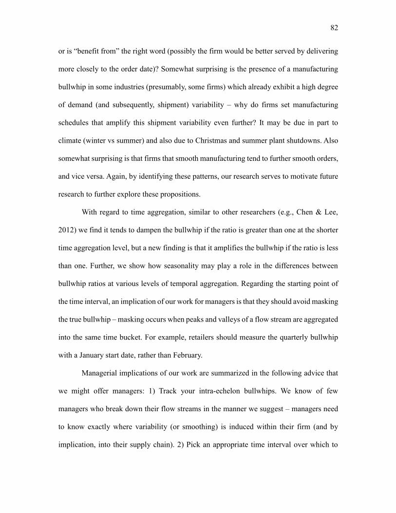
82
or is “benefit from” the right word (possibly the firm would be better served by delivering
more closely to the order date)? Somewhat surprising is the presence of a manufacturing
bullwhip in some industries (presumably, some firms) which already exhibit a high degree
of demand (and subsequently, shipment) variability – why do firms set manufacturing
schedules that amplify this shipment variability even further? It may be due in part to
climate (winter vs summer) and also due to Christmas and summer plant shutdowns. Also
somewhat surprising is that firms that smooth manufacturing tend to further smooth orders,
and vice versa. Again, by identifying these patterns, our research serves to motivate future
research to further explore these propositions.
With regard to time aggregation, similar to other researchers (e.g., Chen & Lee,
2012) we find it tends to dampen the bullwhip if the ratio is greater than one at the shorter
time aggregation level, but a new finding is that it amplifies the bullwhip if the ratio is less
than one. Further, we show how seasonality may play a role in the differences between
bullwhip ratios at various levels of temporal aggregation. Regarding the starting point of
the time interval, an implication of our work for managers is that they should avoid masking
the true bullwhip – masking occurs when peaks and valleys of a flow stream are aggregated
into the same time bucket. For example, retailers should measure the quarterly bullwhip
with a January start date, rather than February.
Managerial implications of our work are summarized in the following advice that
we might offer managers: 1) Track your intra-echelon bullwhips. We know of few
managers who break down their flow streams in the manner we suggest – managers need
to know exactly where variability (or smoothing) is induced within their firm (and by
implication, into their supply chain). 2) Pick an appropriate time interval over which to

83
track your bullwhips, and an appropriate starting point for this interval (see above
paragraph). 3) Understand what drives each of the intra-echelon bullwhips. The
manufacturing bullwhip may be driven by the weather (e.g., higher output may be
achievable in warm-weather months) or conversely, the firm may be able to achieve a
manufacturing antibullwhip by implementing lean operations. But managers should
understand the drivers of each of the intra-echelon bullwhips within their firm – and more
broadly, their supply chain. 4) Rigorously track each intra-echelon bullwhip with an eye
toward continuously driving it down, in an effort to achieve the “ideal” as described at the
outset of section 3.2.
Many complex factors contribute to the challenge facing managers in attempting to
match supply with demand across a distributed supply chain. Understanding and managing
the bullwhip effect is a complex and difficult task. Our work demonstrates the value of
measuring and tracking various intra-echelon bullwhip effects in addition to the overall
inter-echelon bullwhip. Specifically, our approach to decomposing the bullwhip provides
guidance to firms seeking to better manage their shipping, manufacturing, and ordering
activities.
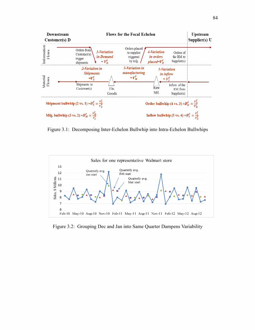
84
Figure 3.1: Decomposing Inter-Echelon Bullwhip into Intra-Echelon Bullwhips
Figure 3.2: Grouping Dec and Jan into Same Quarter Dampens Variability
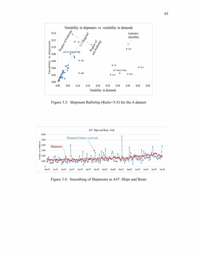
85
Figure 3.3: Shipment Bullwhip (Ratio=Y/X) for the A dataset
Figure 3.4: Smoothing of Shipments in A47: Ships and Boats
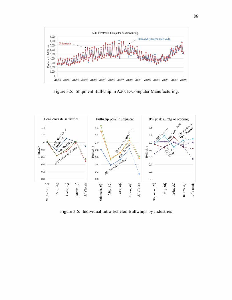
86
Figure 3.5: Shipment Bullwhip in A20: E-Computer Manufacturing.
Figure 3.6: Individual Intra-Echelon Bullwhips by Industries
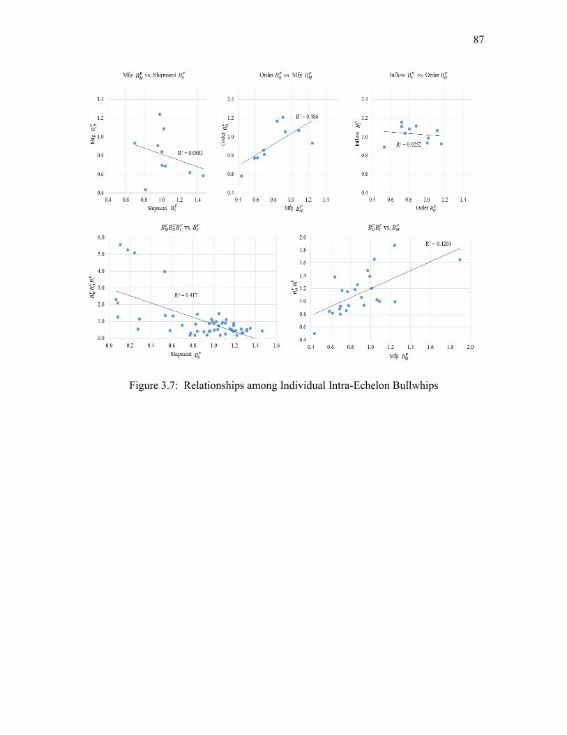
87
Figure 3.7: Relationships among Individual Intra-Echelon Bullwhips
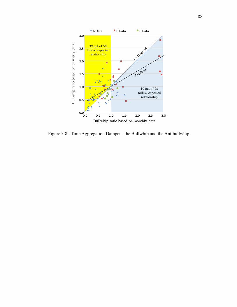
88
Figure 3.8: Time Aggregation Dampens the Bullwhip and the Antibullwhip
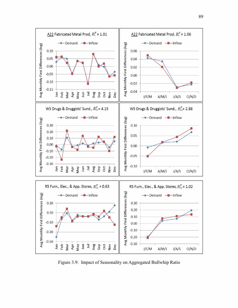
89
Figure 3.9: Impact of Seasonality on Aggregated Bullwhip Ratio
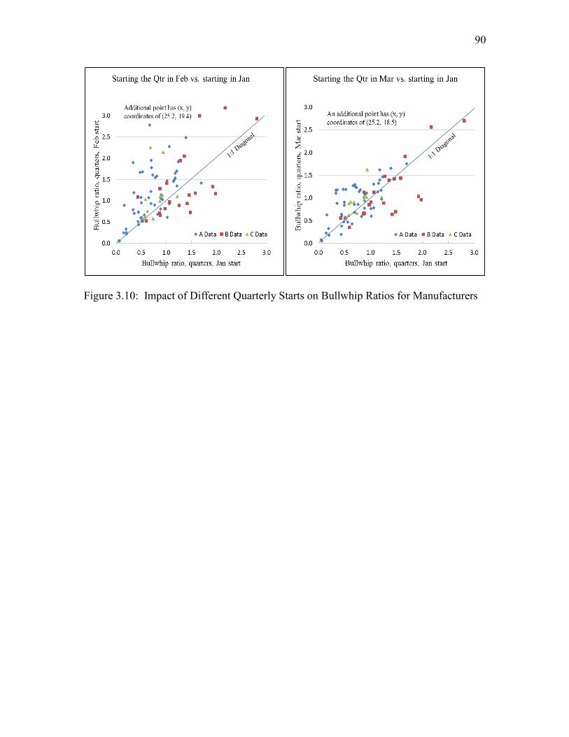
90
Figure 3.10: Impact of Different Quarterly Starts on Bullwhip Ratios for Manufacturers
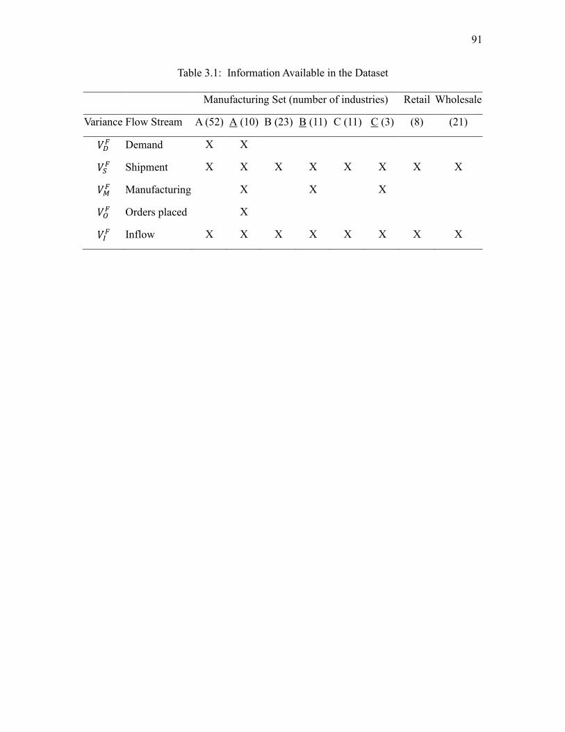
91
Table 3.1: Information Available in the Dataset
Manufacturing Set (number of industries) Retail Wholesale
Variance Flow Stream A (52) A (10) B (23) B (11) C (11) C (3) (8) (21)
𝑉𝐷𝐹 Demand X X
𝑉𝑆𝐹 Shipment X X X X X X X X
𝑉𝑀𝐹 Manufacturing X X X
𝑉𝑂𝐹 Orders placed X
𝑉𝐼𝐹 Inflow X X X X X X X X
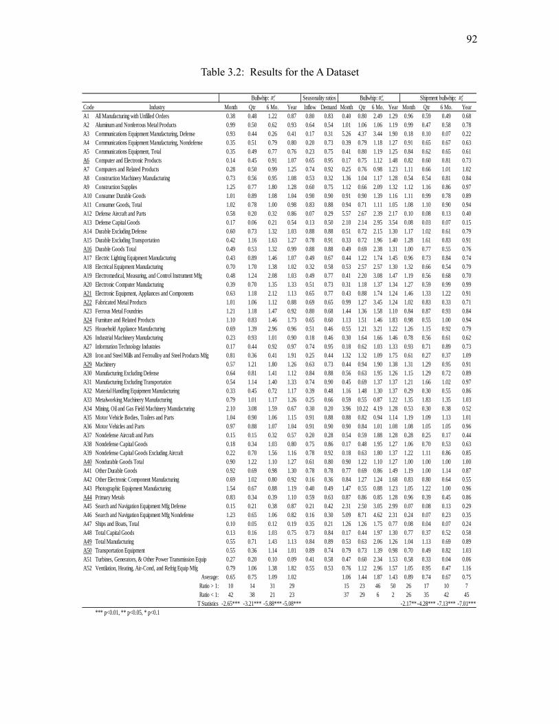
92
Table 3.2: Results for the A Dataset
Code Industry Month Qtr 6 Mo. Year Inflow Demand Month Qtr 6 Mo. Year Month Qtr 6 Mo. Year
A1 All Manufacturing with Unfilled Orders 0.38 0.48 1.22 0.87 0.80 0.83 0.40 0.80 2.49 1.29 0.96 0.59 0.49 0.68
A2 Aluminum and Nonferrous Metal Products 0.99 0.50 0.62 0.93 0.64 0.54 1.01 1.06 1.06 1.19 0.99 0.47 0.58 0.78
A3 Communications Equipment Manufacturing, Defense 0.93 0.44 0.26 0.41 0.17 0.31 5.26 4.37 3.44 1.90 0.18 0.10 0.07 0.22
A4 Communications Equipment Manufacturing, Nondefense 0.35 0.51 0.79 0.80 0.20 0.73 0.39 0.79 1.18 1.27 0.91 0.65 0.67 0.63
A5 Communications Equipment, Total 0.35 0.49 0.77 0.76 0.23 0.75 0.41 0.80 1.19 1.25 0.84 0.62 0.65 0.61
A6 Computer and Electronic Products 0.14 0.45 0.91 1.07 0.65 0.95 0.17 0.75 1.12 1.48 0.82 0.60 0.81 0.73
A7 Computers and Related Products 0.28 0.50 0.99 1.25 0.74 0.92 0.25 0.76 0.98 1.23 1.11 0.66 1.01 1.02
A8 Construction Machinery Manufacturing 0.73 0.56 0.95 1.08 0.53 0.32 1.36 1.04 1.17 1.28 0.54 0.54 0.81 0.84
A9 Construction Supplies 1.25 0.77 1.80 1.28 0.60 0.75 1.12 0.66 2.09 1.32 1.12 1.16 0.86 0.97
A10 Consumer Durable Goods 1.01 0.89 1.08 1.04 0.90 0.90 0.91 0.90 1.39 1.16 1.11 0.99 0.78 0.89
A11 Consumer Goods, Total 1.02 0.78 1.00 0.98 0.83 0.88 0.94 0.71 1.11 1.05 1.08 1.10 0.90 0.94
A12 Defense Aircraft and Parts 0.58 0.20 0.32 0.86 0.07 0.29 5.57 2.67 2.39 2.17 0.10 0.08 0.13 0.40
A13 Defense Capital Goods 0.17 0.06 0.21 0.54 0.13 0.50 2.10 2.14 2.95 3.54 0.08 0.03 0.07 0.15
A14 Durable Excluding Defense 0.60 0.73 1.32 1.03 0.88 0.88 0.51 0.72 2.15 1.30 1.17 1.02 0.61 0.79
A15 Durable Excluding Transportation 0.42 1.16 1.63 1.27 0.78 0.91 0.33 0.72 1.96 1.40 1.28 1.61 0.83 0.91
A16 Durable Goods Total 0.49 0.53 1.32 0.99 0.88 0.88 0.49 0.69 2.38 1.31 1.00 0.77 0.55 0.76
A17 Electric Lighting Equipment Manufacturing 0.43 0.89 1.46 1.07 0.49 0.67 0.44 1.22 1.74 1.45 0.96 0.73 0.84 0.74
A18 Electrical Equipment Manufacturing 0.70 1.70 1.38 1.02 0.32 0.58 0.53 2.57 2.57 1.30 1.32 0.66 0.54 0.79
A19 Electromedical, Measuring, and Control Instrument Mfg 0.48 1.24 2.08 1.03 0.49 0.77 0.41 2.20 3.08 1.47 1.19 0.56 0.68 0.70
A20 Electronic Computer Manufacturing 0.39 0.70 1.35 1.33 0.51 0.73 0.31 1.18 1.37 1.34 1.27 0.59 0.99 0.99
A21 Electronic Equipment, Appliances and Components 0.63 1.18 2.12 1.13 0.65 0.77 0.43 0.88 1.74 1.24 1.46 1.33 1.22 0.91
A22 Fabricated Metal Products 1.01 1.06 1.12 0.88 0.69 0.65 0.99 1.27 3.45 1.24 1.02 0.83 0.33 0.71
A23 Ferrous Metal Foundries 1.21 1.18 1.47 0.92 0.80 0.68 1.44 1.36 1.58 1.10 0.84 0.87 0.93 0.84
A24 Furniture and Related Products 1.10 0.83 1.46 1.73 0.65 0.60 1.13 1.51 1.46 1.83 0.98 0.55 1.00 0.94
A25 Household Appliance Manufacturing 0.69 1.39 2.96 0.96 0.51 0.46 0.55 1.21 3.21 1.22 1.26 1.15 0.92 0.79
A26 Industrial Machinery Manufacturing 0.23 0.93 1.01 0.90 0.18 0.46 0.30 1.64 1.66 1.46 0.78 0.56 0.61 0.62
A27 Information Technology Industries 0.17 0.44 0.92 0.97 0.74 0.95 0.18 0.62 1.03 1.33 0.93 0.71 0.89 0.73
A28 Iron and Steel Mills and Ferroalloy and Steel Products Mfg 0.81 0.36 0.41 1.91 0.25 0.44 1.32 1.32 1.09 1.75 0.61 0.27 0.37 1.09
A29 Machinery 0.57 1.21 1.80 1.26 0.63 0.73 0.44 0.94 1.90 1.38 1.31 1.29 0.95 0.91
A30 Manufacturing Excluding Defense 0.64 0.81 1.41 1.12 0.84 0.88 0.56 0.63 1.95 1.26 1.15 1.29 0.72 0.89
A31 Manufacturing Excluding Transportation 0.54 1.14 1.40 1.33 0.74 0.90 0.45 0.69 1.37 1.37 1.21 1.66 1.02 0.97
A32 Material Handling Equipment Manufacturing 0.33 0.45 0.72 1.17 0.39 0.48 1.16 1.48 1.30 1.37 0.29 0.30 0.55 0.86
A33 Metalworking Machinery Manufacturing 0.79 1.01 1.17 1.26 0.25 0.66 0.59 0.55 0.87 1.22 1.35 1.83 1.35 1.03
A34 Mining, Oil and Gas Field Machinery Manufacturing 2.10 3.08 1.59 0.67 0.30 0.20 3.96 10.22 4.19 1.28 0.53 0.30 0.38 0.52
A35 Motor Vehicle Bodies, Trailers and Parts 1.04 0.90 1.06 1.15 0.91 0.88 0.88 0.82 0.94 1.14 1.19 1.09 1.13 1.01
A36 Motor Vehicles and Parts 0.97 0.88 1.07 1.04 0.91 0.90 0.90 0.84 1.01 1.08 1.08 1.05 1.05 0.96
A37 Nondefense Aircraft and Parts 0.15 0.15 0.32 0.57 0.20 0.28 0.54 0.59 1.88 1.28 0.28 0.25 0.17 0.44
A38 Nondefense Capital Goods 0.18 0.34 1.03 0.80 0.75 0.86 0.17 0.48 1.95 1.27 1.06 0.70 0.53 0.63
A39 Nondefense Capital Goods Excluding Aircraft 0.22 0.70 1.56 1.16 0.78 0.92 0.18 0.63 1.80 1.37 1.22 1.11 0.86 0.85
A40 Nondurable Goods Total 0.90 1.22 1.10 1.27 0.61 0.80 0.90 1.22 1.10 1.27 1.00 1.00 1.00 1.00
A41 Other Durable Goods 0.92 0.69 0.98 1.30 0.78 0.78 0.77 0.69 0.86 1.49 1.19 1.00 1.14 0.87
A42 Other Electronic Component Manufacturing 0.69 1.02 0.80 0.92 0.16 0.36 0.84 1.27 1.24 1.68 0.83 0.80 0.64 0.55
A43 Photographic Equipment Manufacturing 1.54 0.67 0.88 1.19 0.40 0.49 1.47 0.55 0.88 1.23 1.05 1.22 1.00 0.96
A44 Primary Metals 0.83 0.34 0.39 1.10 0.59 0.63 0.87 0.86 0.85 1.28 0.96 0.39 0.45 0.86
A45 Search and Navigation Equipment Mfg Defense 0.15 0.21 0.38 0.87 0.21 0.42 2.31 2.50 3.05 2.99 0.07 0.08 0.13 0.29
A46 Search and Navigation Equipment Mfg Nondefense 1.23 0.65 1.06 0.82 0.16 0.30 5.09 8.71 4.62 2.31 0.24 0.07 0.23 0.35
A47 Ships and Boats, Total 0.10 0.05 0.12 0.19 0.35 0.21 1.26 1.26 1.75 0.77 0.08 0.04 0.07 0.24
A48 Total Capital Goods 0.13 0.16 1.03 0.75 0.73 0.84 0.17 0.44 1.97 1.30 0.77 0.37 0.52 0.58
A49 Total Manufacturing 0.55 0.71 1.43 1.13 0.84 0.89 0.53 0.63 2.06 1.26 1.04 1.13 0.69 0.89
A50 Transportation Equipment 0.55 0.36 1.14 1.01 0.89 0.74 0.79 0.73 1.39 0.98 0.70 0.49 0.82 1.03
A51 Turbines, Generators, & Other Power Transmission Equip 0.27 0.20 0.10 0.09 0.41 0.58 0.47 0.60 2.34 1.53 0.58 0.33 0.04 0.06
A52 Ventilation, Heating, Air-Cond, and Refrig Equip Mfg 0.79 1.06 1.38 1.82 0.55 0.53 0.76 1.12 2.96 1.57 1.05 0.95 0.47 1.16
Average: 0.65 0.75 1.09 1.02 1.06 1.44 1.87 1.43 0.89 0.74 0.67 0.75
Ratio > 1: 10 14 31 29 15 23 46 50 26 17 10 7
Ratio < 1: 42 38 21 23 37 29 6 2 26 35 42 45
T Statistics -2.65*** -3.21*** -5.88*** -5.08*** -2.17** -4.28*** -7.13*** -7.01***
*** p<0.01, ** p<0.05, * p<0.1
Bullwhip: Bullwhip: Seasonality ratios Shipment bullwhip:𝐵∗𝐹 𝐵∗∗
𝐹 𝐵𝑆𝐹
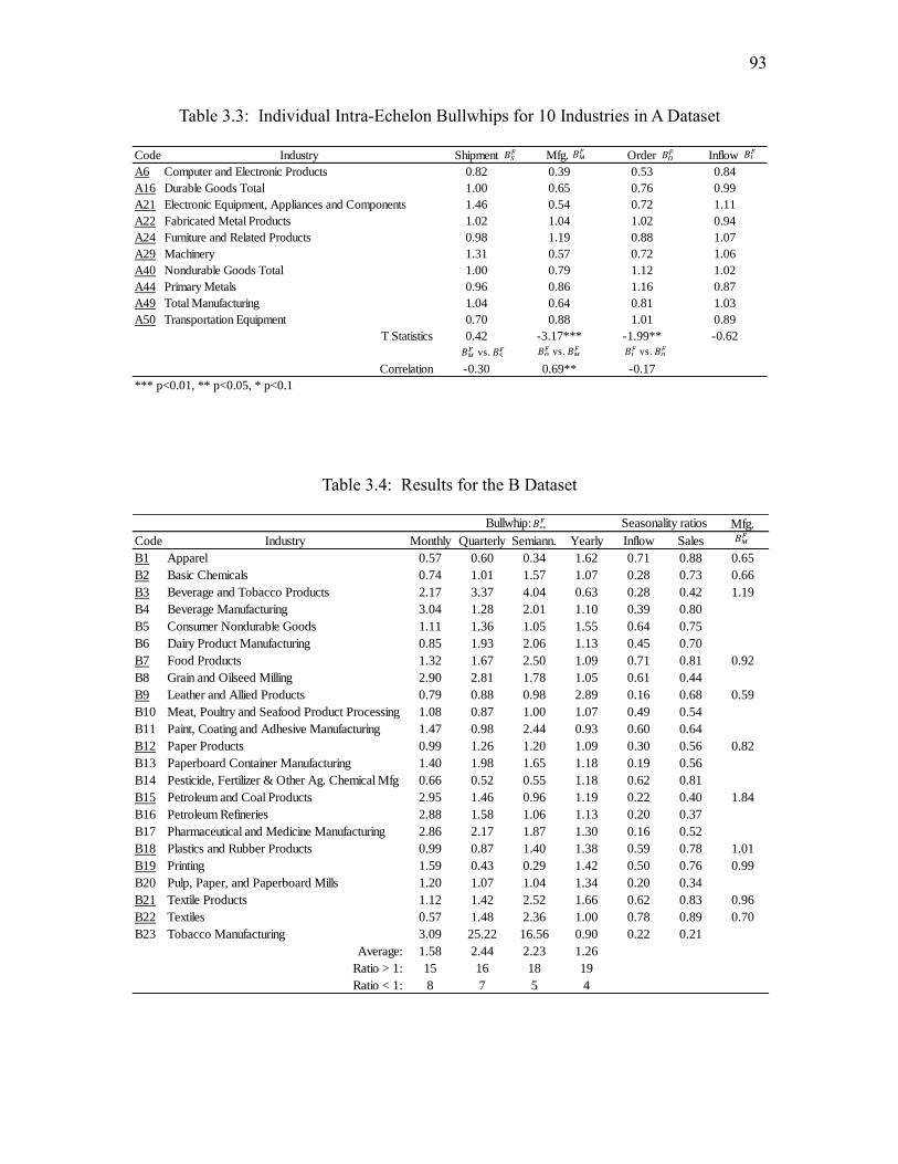
93
Table 3.3: Individual Intra-Echelon Bullwhips for 10 Industries in A Dataset
Table 3.4: Results for the B Dataset
Code Industry Shipment Mfg. Order Inflow
A6 Computer and Electronic Products 0.82 0.39 0.53 0.84
A16 Durable Goods Total 1.00 0.65 0.76 0.99
A21 Electronic Equipment, Appliances and Components 1.46 0.54 0.72 1.11
A22 Fabricated Metal Products 1.02 1.04 1.02 0.94
A24 Furniture and Related Products 0.98 1.19 0.88 1.07
A29 Machinery 1.31 0.57 0.72 1.06
A40 Nondurable Goods Total 1.00 0.79 1.12 1.02
A44 Primary Metals 0.96 0.86 1.16 0.87
A49 Total Manufacturing 1.04 0.64 0.81 1.03
A50 Transportation Equipment 0.70 0.88 1.01 0.89
T Statistics 0.42 -3.17*** -1.99** -0.62
Correlation -0.30 0.69** -0.17
*** p<0.01, ** p<0.05, * p<0.1
𝐵𝑆𝐹 𝐵𝑀
𝐹 𝐵𝑂𝐹 𝐵𝐼
𝐹
𝐵𝑂𝐹 vs. 𝐵𝑀
𝐹𝐵𝑀𝐹 vs. 𝐵𝑆
𝐹 𝐵𝐼𝐹 vs. 𝐵𝑂
𝐹
Mfg.
Code Industry Monthly Quarterly Semiann. Yearly Inflow Sales
B1 Apparel 0.57 0.60 0.34 1.62 0.71 0.88 0.65
B2 Basic Chemicals 0.74 1.01 1.57 1.07 0.28 0.73 0.66
B3 Beverage and Tobacco Products 2.17 3.37 4.04 0.63 0.28 0.42 1.19
B4 Beverage Manufacturing 3.04 1.28 2.01 1.10 0.39 0.80
B5 Consumer Nondurable Goods 1.11 1.36 1.05 1.55 0.64 0.75
B6 Dairy Product Manufacturing 0.85 1.93 2.06 1.13 0.45 0.70
B7 Food Products 1.32 1.67 2.50 1.09 0.71 0.81 0.92
B8 Grain and Oilseed Milling 2.90 2.81 1.78 1.05 0.61 0.44
B9 Leather and Allied Products 0.79 0.88 0.98 2.89 0.16 0.68 0.59
B10 Meat, Poultry and Seafood Product Processing 1.08 0.87 1.00 1.07 0.49 0.54
B11 Paint, Coating and Adhesive Manufacturing 1.47 0.98 2.44 0.93 0.60 0.64
B12 Paper Products 0.99 1.26 1.20 1.09 0.30 0.56 0.82
B13 Paperboard Container Manufacturing 1.40 1.98 1.65 1.18 0.19 0.56
B14 Pesticide, Fertilizer & Other Ag. Chemical Mfg 0.66 0.52 0.55 1.18 0.62 0.81
B15 Petroleum and Coal Products 2.95 1.46 0.96 1.19 0.22 0.40 1.84
B16 Petroleum Refineries 2.88 1.58 1.06 1.13 0.20 0.37
B17 Pharmaceutical and Medicine Manufacturing 2.86 2.17 1.87 1.30 0.16 0.52
B18 Plastics and Rubber Products 0.99 0.87 1.40 1.38 0.59 0.78 1.01
B19 Printing 1.59 0.43 0.29 1.42 0.50 0.76 0.99
B20 Pulp, Paper, and Paperboard Mills 1.20 1.07 1.04 1.34 0.20 0.34
B21 Textile Products 1.12 1.42 2.52 1.66 0.62 0.83 0.96
B22 Textiles 0.57 1.48 2.36 1.00 0.78 0.89 0.70
B23 Tobacco Manufacturing 3.09 25.22 16.56 0.90 0.22 0.21
Average: 1.58 2.44 2.23 1.26
Ratio > 1: 15 16 18 19
Ratio < 1: 8 7 5 4
Bullwhip: Seasonality ratios𝐵𝑀
𝐹
𝐵∗∗𝐹
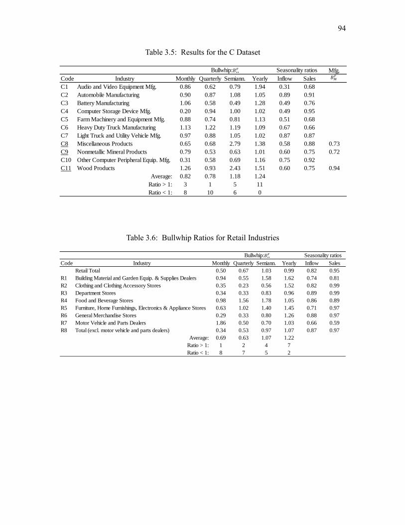
94
Table 3.5: Results for the C Dataset
Table 3.6: Bullwhip Ratios for Retail Industries
Mfg.
Code Industry Monthly Quarterly Semiann. Yearly Inflow Sales
C1 Audio and Video Equipment Mfg. 0.86 0.62 0.79 1.94 0.31 0.68
C2 Automobile Manufacturing 0.90 0.87 1.08 1.05 0.89 0.91
C3 Battery Manufacturing 1.06 0.58 0.49 1.28 0.49 0.76
C4 Computer Storage Device Mfg. 0.20 0.94 1.00 1.02 0.49 0.95
C5 Farm Machinery and Equipment Mfg. 0.88 0.74 0.81 1.13 0.51 0.68
C6 Heavy Duty Truck Manufacturing 1.13 1.22 1.19 1.09 0.67 0.66
C7 Light Truck and Utility Vehicle Mfg. 0.97 0.88 1.05 1.02 0.87 0.87
C8 Miscellaneous Products 0.65 0.68 2.79 1.38 0.58 0.88 0.73
C9 Nonmetallic Mineral Products 0.79 0.53 0.63 1.01 0.60 0.75 0.72
C10 Other Computer Peripheral Equip. Mfg. 0.31 0.58 0.69 1.16 0.75 0.92
C11 Wood Products 1.26 0.93 2.43 1.51 0.60 0.75 0.94
Average: 0.82 0.78 1.18 1.24
Ratio > 1: 3 1 5 11
Ratio < 1: 8 10 6 0
Bullwhip: Seasonality ratios𝐵∗∗𝐹
𝐵𝑀𝐹
Code Industry Monthly Quarterly Semiann. Yearly Inflow Sales
Retail Total 0.50 0.67 1.03 0.99 0.82 0.95
R1 Building Material and Garden Equip. & Supplies Dealers 0.94 0.55 1.58 1.62 0.74 0.81
R2 Clothing and Clothing Accessory Stores 0.35 0.23 0.56 1.52 0.82 0.99
R3 Department Stores 0.34 0.33 0.83 0.96 0.89 0.99
R4 Food and Beverage Stores 0.98 1.56 1.78 1.05 0.86 0.89
R5 Furniture, Home Furnishings, Electronics & Appliance Stores 0.63 1.02 1.40 1.45 0.71 0.97
R6 General Merchandise Stores 0.29 0.33 0.80 1.26 0.88 0.97
R7 Motor Vehicle and Parts Dealers 1.86 0.50 0.70 1.03 0.66 0.59
R8 Total (excl. motor vehicle and parts dealers) 0.34 0.53 0.97 1.07 0.87 0.97
Average: 0.69 0.63 1.07 1.22
Ratio > 1: 1 2 4 7
Ratio < 1: 8 7 5 2
Bullwhip: Seasonality ratios𝐵∗∗𝐹
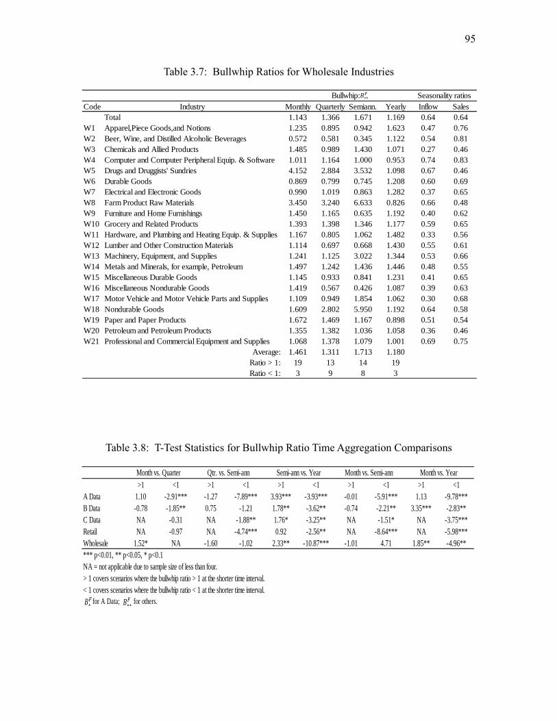
95
Table 3.7: Bullwhip Ratios for Wholesale Industries
Table 3.8: T-Test Statistics for Bullwhip Ratio Time Aggregation Comparisons
Code Industry Monthly Quarterly Semiann. Yearly Inflow Sales
Total 1.143 1.366 1.671 1.169 0.64 0.64
W1 Apparel,Piece Goods,and Notions 1.235 0.895 0.942 1.623 0.47 0.76
W2 Beer, Wine, and Distilled Alcoholic Beverages 0.572 0.581 0.345 1.122 0.54 0.81
W3 Chemicals and Allied Products 1.485 0.989 1.430 1.071 0.27 0.46
W4 Computer and Computer Peripheral Equip. & Software 1.011 1.164 1.000 0.953 0.74 0.83
W5 Drugs and Druggists' Sundries 4.152 2.884 3.532 1.098 0.67 0.46
W6 Durable Goods 0.869 0.799 0.745 1.208 0.60 0.69
W7 Electrical and Electronic Goods 0.990 1.019 0.863 1.282 0.37 0.65
W8 Farm Product Raw Materials 3.450 3.240 6.633 0.826 0.66 0.48
W9 Furniture and Home Furnishings 1.450 1.165 0.635 1.192 0.40 0.62
W10 Grocery and Related Products 1.393 1.398 1.346 1.177 0.59 0.65
W11 Hardware, and Plumbing and Heating Equip. & Supplies 1.167 0.805 1.062 1.482 0.33 0.56
W12 Lumber and Other Construction Materials 1.114 0.697 0.668 1.430 0.55 0.61
W13 Machinery, Equipment, and Supplies 1.241 1.125 3.022 1.344 0.53 0.66
W14 Metals and Minerals, for example, Petroleum 1.497 1.242 1.436 1.446 0.48 0.55
W15 Miscellaneous Durable Goods 1.145 0.933 0.841 1.231 0.41 0.65
W16 Miscellaneous Nondurable Goods 1.419 0.567 0.426 1.087 0.39 0.63
W17 Motor Vehicle and Motor Vehicle Parts and Supplies 1.109 0.949 1.854 1.062 0.30 0.68
W18 Nondurable Goods 1.609 2.802 5.950 1.192 0.64 0.58
W19 Paper and Paper Products 1.672 1.469 1.167 0.898 0.51 0.54
W20 Petroleum and Petroleum Products 1.355 1.382 1.036 1.058 0.36 0.46
W21 Professional and Commercial Equipment and Supplies 1.068 1.378 1.079 1.001 0.69 0.75
Average: 1.461 1.311 1.713 1.180
Ratio > 1: 19 13 14 19
Ratio < 1: 3 9 8 3
Bullwhip: Seasonality ratios𝐵∗∗𝐹
>1 <1 >1 <1 >1 <1 >1 <1 >1 <1
A Data 1.10 -2.91*** -1.27 -7.89*** 3.93*** -3.93*** -0.01 -5.91*** 1.13 -9.78***
B Data -0.78 -1.85** 0.75 -1.21 1.78** -3.62** -0.74 -2.21** 3.35*** -2.83**
C Data NA -0.31 NA -1.88** 1.76* -3.25** NA -1.51* NA -3.75***
Retail NA -0.97 NA -4.74*** 0.92 -2.56** NA -8.64*** NA -5.98***
Wholesale 1.52* NA -1.60 -1.02 2.33** -10.87*** -1.01 4.71 1.85** -4.96**
*** p<0.01, ** p<0.05, * p<0.1
NA = not applicable due to sample size of less than four.
> 1 covers scenarios where the bullwhip ratio > 1 at the shorter time interval.
< 1 covers scenarios where the bullwhip ratio < 1 at the shorter time interval.
for A Data; for others.
Month vs. Quarter Qtr. vs. Semi-ann Semi-ann vs. Year Month vs. Semi-ann Month vs. Year
𝐵∗𝐹 𝐵∗∗
𝐹
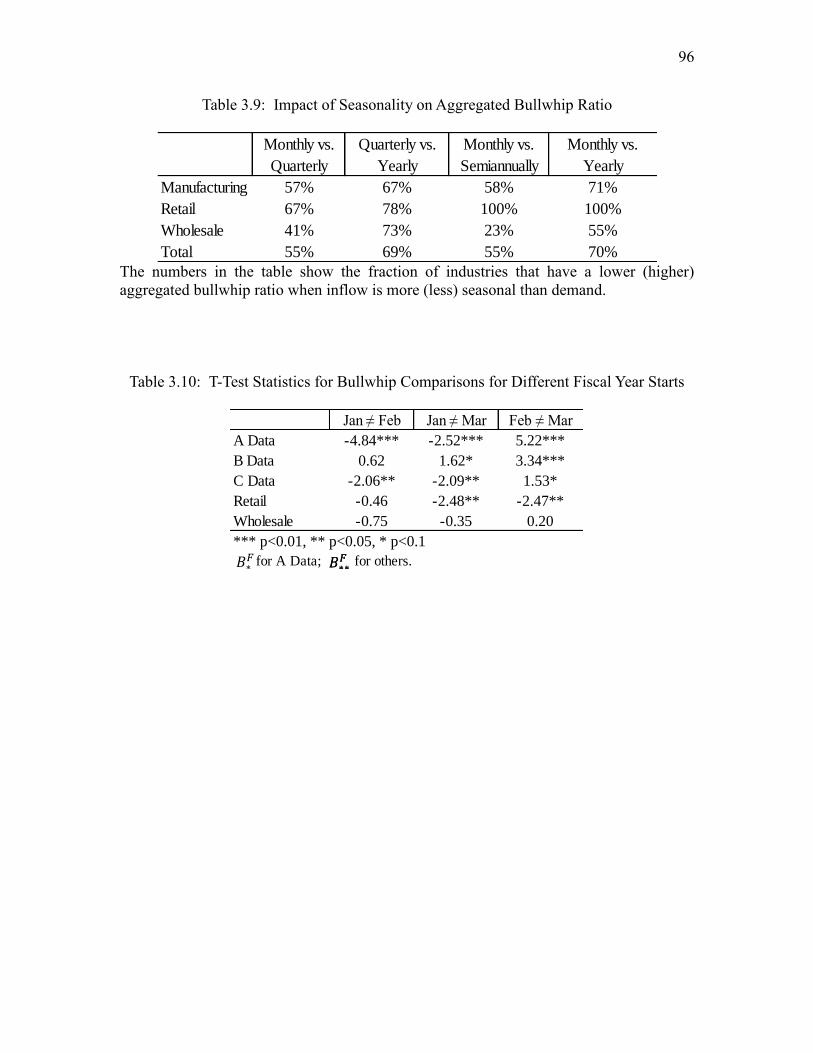
96
Table 3.9: Impact of Seasonality on Aggregated Bullwhip Ratio
The numbers in the table show the fraction of industries that have a lower (higher)
aggregated bullwhip ratio when inflow is more (less) seasonal than demand.
Table 3.10: T-Test Statistics for Bullwhip Comparisons for Different Fiscal Year Starts
Monthly vs. Quarterly vs. Monthly vs. Monthly vs.
Quarterly Yearly Semiannually Yearly
Manufacturing 57% 67% 58% 71%
Retail 67% 78% 100% 100%
Wholesale 41% 73% 23% 55%
Total 55% 69% 55% 70%
Jan ≠ Feb Jan ≠ Mar Feb ≠ Mar
A Data -4.84*** -2.52*** 5.22***
B Data 0.62 1.62* 3.34***
C Data -2.06** -2.09** 1.53*
Retail -0.46 -2.48** -2.47**
Wholesale -0.75 -0.35 0.20
*** p<0.01, ** p<0.05, * p<0.1
for A Data; for others.𝐵∗𝐹 𝐵∗∗
𝐹𝐵∗∗𝐹
CHAPTER 4
BULLWHIP EFFECT IN A PHARMACEUTICAL SUPPLY CHAIN
4.1 Introduction
A significant advancement in supply chain management in the past three decades is
the identification and management of the bullwhip effect. In a seminal paper, Lee et al.
(1997a) define the bullwhip effect as “the phenomenon where orders to the supplier tend
to have larger variance than sales to the buyer (i.e., demand distortion), and the distortion
propagates upstream in an amplified form (i.e., variance amplification)” (p. 546). The
bullwhip effect has been observed in many firms and industries: Barilla’s pasta supply
chain (Hammond, 1994), machine tool industry (Anderson et al., 2000), European
convenience foods supply chain (Fransoo & Wouters, 2000), a supermarket chain in Spain
(Lai, 2005), Philips electronics (De Kok et al., 2005), semiconductor equipment industry
(Terwiesch et al., 2005), and U.S. industries (Cachon et al., 2007).
The bullwhip effect leads to significant supply chain inefficiencies such as
excessive capital investment in inventory, mismatched production schedules, poor
customer service, lost revenues, misguided capacity planning, and additional transportation
costs (e.g., Sterman, 1989; Lee et al., 1997b; Jin et al., 2015a). As a result, taming the
bullwhip has attracted much attention from both researchers and practitioners. For example,
Lee et al. (1997a) identify four causes of the bullwhip effect and suggest several strategies

98
to mitigate its detrimental impact.
Although there is a growing literature of empirical studies on the bullwhip effect,
there are several challenges in empirical investigation of the effect. First, Chen and Lee
(2012) point out that two major definitions of bullwhip effect measurement have been used
in the literature: information-based definition and material-based definition. The
information-based definition originating from Lee et al. (1997a) compares order variance
with demand variance. It has been widely used in theoretical analysis. The material-based
definition that is used in most empirical studies compares the variance of order receipts
with that of sales. These two definitions differ in concept and are not necessarily good
approximations of each other. Hence, empirical studies on bullwhip effect using material-
based definition may not have a direct bearing on the theoretical models that use
information-based definition. Second, analytical analysis of the bullwhip effect is usually
based on a single product and order decision period. However, due to data availability
issues, most empirical studies measure the bullwhip effect based on aggregated products
and aggregated time to a month or longer. Measuring the bullwhip effect in aggregate data
may cause potential biases in estimation (Chen & Lee, 2012). Whether aggregation
amplifies, preserves, or dampens the bullwhip effect is an important question to explore.
For example, if the data aggregation masks the bullwhip effect, then the managers who
make financial planning and investment decisions based on quarterly or yearly firm-level
data will probably overlook the severity of monthly product-level bullwhip effect. But it is
monthly information at product level that defines much of a firm’s operations management.
Third, the bullwhip effect is a phenomenon on the entire supply chain. Bullwhip effect
estimation requires information such as order and demand data from each echelon along

99
the supply chain to keep track of individual products. It is a formidable task to collect this
information. To the best of our knowledge, no prior work manages to do this.
We address these empirical challenges by analyzing a proprietary dataset collected
from a multiechelon pharmaceutical supply chain and make the following contributions to
the literature. First, we measure the bullwhip effect based on information flows and
compare it with that based on material flows. Second, we report the bullwhip effect in a
supply chain at the product level and in fine time buckets such as monthly as defined in
analytical papers. Third, we explore how data aggregation affects the bullwhip
measurement. Specifically, we investigate whether product aggregation and temporal
aggregation preserve or mask the bullwhip effect. Fourth, we measure the bullwhip effect
across different echelons of a supply chain, rather than across a compilation of individual
firms or industries. Fifth, we examine some drivers of the bullwhip effect such as price
fluctuation, replenishment lead time, and inventory.
Our key findings are the following: (1) Distributors exhibit a prevalent and
intensive bullwhip effect. (2) Manufacturer exhibits a less intensive bullwhip effect than
distributors and makes production smoother than demand for some products. (3) The
bullwhip measure based on order receipt variance underestimates the one based on order
variance. (4) Products that have a flatter demand are more likely to exhibit the bullwhip
effect. (5) Product aggregation and time aggregation tend to mask the bullwhip effect in
some cases. (6) Price variation, inventory, and replenishment lead time are three prominent
factors related to the bullwhip effect.
The rest of this chapter is organized as follows. Section 4.2 provides a brief survey
of the related literature. Section 4.3 outlines our hypotheses. Section 4.4 summarizes
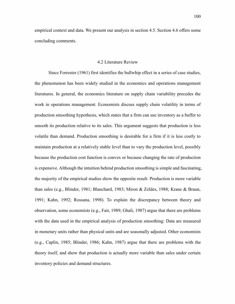
100
empirical context and data. We present our analysis in section 4.5. Section 4.6 offers some
concluding comments.
4.2 Literature Review
Since Forrester (1961) first identifies the bullwhip effect in a series of case studies,
the phenomenon has been widely studied in the economics and operations management
literatures. In general, the economics literature on supply chain variability precedes the
work in operations management. Economists discuss supply chain volatility in terms of
production smoothing hypothesis, which states that a firm can use inventory as a buffer to
smooth its production relative to its sales. This argument suggests that production is less
volatile than demand. Production smoothing is desirable for a firm if it is less costly to
maintain production at a relatively stable level than to vary the production level, possibly
because the production cost function is convex or because changing the rate of production
is expensive. Although the intuition behind production smoothing is simple and fascinating,
the majority of the empirical studies show the opposite result: Production is more variable
than sales (e.g., Blinder, 1981; Blanchard, 1983; Miron & Zeldes, 1988; Krane & Braun,
1991; Kahn, 1992; Rossana, 1998). To explain the discrepancy between theory and
observation, some economists (e.g., Fair, 1989; Ghali, 1987) argue that there are problems
with the data used in the empirical analysis of production smoothing: Data are measured
in monetary units rather than physical units and are seasonally adjusted. Other economists
(e.g., Caplin, 1985; Blinder, 1986; Kahn, 1987) argue that there are problems with the
theory itself, and show that production is actually more variable than sales under certain
inventory policies and demand structures.
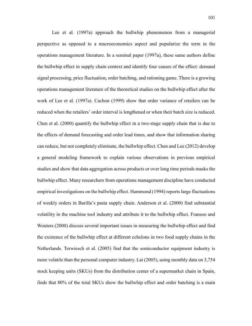
101
Lee et al. (1997a) approach the bullwhip phenomenon from a managerial
perspective as opposed to a macroeconomics aspect and popularize the term in the
operations management literature. In a seminal paper (1997a), these same authors define
the bullwhip effect in supply chain context and identify four causes of the effect: demand
signal processing, price fluctuation, order batching, and rationing game. There is a growing
operations management literature of the theoretical studies on the bullwhip effect after the
work of Lee et al. (1997a). Cachon (1999) show that order variance of retailers can be
reduced when the retailers’ order interval is lengthened or when their batch size is reduced.
Chen et al. (2000) quantify the bullwhip effect in a two-stage supply chain that is due to
the effects of demand forecasting and order lead times, and show that information sharing
can reduce, but not completely eliminate, the bullwhip effect. Chen and Lee (2012) develop
a general modeling framework to explain various observations in previous empirical
studies and show that data aggregation across products or over long time periods masks the
bullwhip effect. Many researchers from operations management discipline have conducted
empirical investigations on the bullwhip effect. Hammond (1994) reports large fluctuations
of weekly orders in Barilla’s pasta supply chain. Anderson et al. (2000) find substantial
volatility in the machine tool industry and attribute it to the bullwhip effect. Fransoo and
Wouters (2000) discuss several important issues in measuring the bullwhip effect and find
the existence of the bullwhip effect at different echelons in two food supply chains in the
Netherlands. Terwiesch et al. (2005) find that the semiconductor equipment industry is
more volatile than the personal computer industry. Lai (2005), using monthly data on 3,754
stock keeping units (SKUs) from the distribution center of a supermarket chain in Spain,
finds that 80% of the total SKUs show the bullwhip effect and order batching is a main
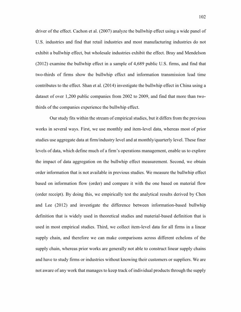
102
driver of the effect. Cachon et al. (2007) analyze the bullwhip effect using a wide panel of
U.S. industries and find that retail industries and most manufacturing industries do not
exhibit a bullwhip effect, but wholesale industries exhibit the effect. Bray and Mendelson
(2012) examine the bullwhip effect in a sample of 4,689 public U.S. firms, and find that
two-thirds of firms show the bullwhip effect and information transmission lead time
contributes to the effect. Shan et al. (2014) investigate the bullwhip effect in China using a
dataset of over 1,200 public companies from 2002 to 2009, and find that more than two-
thirds of the companies experience the bullwhip effect.
Our study fits within the stream of empirical studies, but it differs from the previous
works in several ways. First, we use monthly and item-level data, whereas most of prior
studies use aggregate data at firm/industry level and at monthly/quarterly level. These finer
levels of data, which define much of a firm’s operations management, enable us to explore
the impact of data aggregation on the bullwhip effect measurement. Second, we obtain
order information that is not available in previous studies. We measure the bullwhip effect
based on information flow (order) and compare it with the one based on material flow
(order receipt). By doing this, we empirically test the analytical results derived by Chen
and Lee (2012) and investigate the difference between information-based bullwhip
definition that is widely used in theoretical studies and material-based definition that is
used in most empirical studies. Third, we collect item-level data for all firms in a linear
supply chain, and therefore we can make comparisons across different echelons of the
supply chain, whereas prior works are generally not able to construct linear supply chains
and have to study firms or industries without knowing their customers or suppliers. We are
not aware of any work that manages to keep track of individual products through the supply
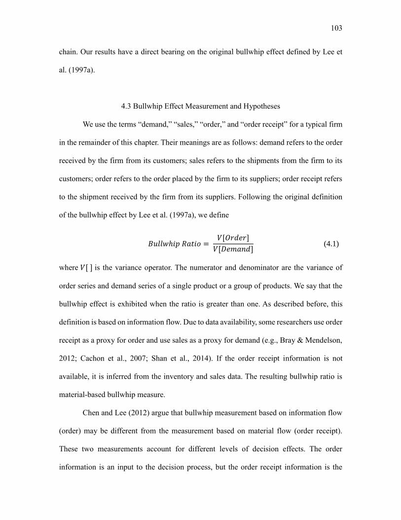
103
chain. Our results have a direct bearing on the original bullwhip effect defined by Lee et
al. (1997a).
4.3 Bullwhip Effect Measurement and Hypotheses
We use the terms “demand,” “sales,” “order,” and “order receipt” for a typical firm
in the remainder of this chapter. Their meanings are as follows: demand refers to the order
received by the firm from its customers; sales refers to the shipments from the firm to its
customers; order refers to the order placed by the firm to its suppliers; order receipt refers
to the shipment received by the firm from its suppliers. Following the original definition
of the bullwhip effect by Lee et al. (1997a), we define
𝐵𝑢𝑙𝑙𝑤ℎ𝑖𝑝 𝑅𝑎𝑡𝑖𝑜 =
𝑉[𝑂𝑟𝑑𝑒𝑟]
𝑉[𝐷𝑒𝑚𝑎𝑛𝑑] (4.1)
where 𝑉[ ] is the variance operator. The numerator and denominator are the variance of
order series and demand series of a single product or a group of products. We say that the
bullwhip effect is exhibited when the ratio is greater than one. As described before, this
definition is based on information flow. Due to data availability, some researchers use order
receipt as a proxy for order and use sales as a proxy for demand (e.g., Bray & Mendelson,
2012; Cachon et al., 2007; Shan et al., 2014). If the order receipt information is not
available, it is inferred from the inventory and sales data. The resulting bullwhip ratio is
material-based bullwhip measure.
Chen and Lee (2012) argue that bullwhip measurement based on information flow
(order) may be different from the measurement based on material flow (order receipt).
These two measurements account for different levels of decision effects. The order
information is an input to the decision process, but the order receipt information is the
104
outcome of the decision process. The bullwhip effect based on material flow is the
consequence of that based on information flow. Chen and Lee (2012) show analytically
that the variance of order receipt sequence is less than that of order sequence. The intuition
is that the downstream orders are truncated by the upstream order-fulfillment capacity, so
the order receipt stream appears less variable. Using the order receipt data as a proxy for
the order data will underestimate the original order variance. We therefore formulate the
following hypothesis:
HYPOTHESIS 1 (H1). The bullwhip ratio based on order receipt variance is lower
than that based on order variance.
Researchers in economics and operations management have explored the impact of
data aggregation across products. Caplin (1985) shows that aggregation across products
preserves the bullwhip effect under (𝑆, 𝑠) inventory policy no matter the correlation
structure of demand. Fransoo and Wouters (2000) show that the same basic data can lead
to different bullwhip measurements, dependent on the sequence of aggregation. Cachon et
al. (2007) write that “Whether aggregation preserves or masks the bullwhip effect or
production smoothing depends on the correlation of production and demand across the
units being aggregate (firms, products, etc.) and on the particular causes of amplification
in place” (p. 477). Using a theoretical model, Chen and Lee (2012) give a rigorous
treatment of the product aggregation issue, and show that the bullwhip effect tends to be
masked under product aggregation. We propose the following hypothesis:
HYPOTHESIS 2 (H2). The bullwhip ratio is smaller at the group/family level than
at the individual product level.
In theoretical studies on the bullwhip effect, researchers derive the bullwhip
105
measure through specific assumptions on the order and demand distribution function.
However, there is usually no information on the distribution function when researchers
conduct empirical investigations on the bullwhip effect. We need to determine an
appropriate time window (e.g., weekly, monthly, or quarterly) to calculate the variances of
order and demand. Fransoo and Wouters (2000) suggest that the appropriate aggregation
over time should depend on the specific problem under study. Chen and Lee (2012) argue
that it is important to measure bullwhip effect at the appropriate time unit for supply chain
cost assessment purposes. Chen and Lee (2012) develop an analytical model to demonstrate
that “aggregating data over relatively long time periods can mask the bullwhip effect” (p.
772). More specifically, they show that under a first-order autoregressive moving average
(ARMA (1, 1)) demand model, if the bullwhip ratio is greater than one, then the ratio will
decrease monotonically to one as the aggregated time period increases. Thus, we propose
the following hypothesis:
HYPOTHESIS 3 (H3). The bullwhip ratio decreases as the aggregation time period
increases.
Lee et al. (1997a) define the bullwhip effect as a supply chain phenomenon where
the demand variability increases from downstream echelons to upstream echelons.
Empirical findings are mixed. Hammond (1994) reports large fluctuations of order
quantities in Barilla’s pasta supply chain. Lee et al. (1997b) observe amplified volatility in
orders in diaper supply chain of Procter and Gamble and in Hewlett-Pachard’s printer
supply chain. However, Cachon et al. (2007) find that retail industries and most
manufacturing industries do not exhibit the bullwhip effect, but the wholesale industries
exhibit the effect. Furthermore, they observe that manufacturing industries (upstream
106
echelon) do not experience greater demand variance than retail industries (downstream
echelon). We construct a linear supply chain from our unique dataset and explore whether
the demand variability amplifies along this three-echelon supply chain. We therefore test
the following hypothesis:
HYPOTHESIS 4 (H4). The firm at upstream stage experiences a larger demand
variability than that at downstream stage.
Price fluctuation is identified as a cause of the bullwhip effect in prior literature.
Blinder (1986) proposes the cost shocks as an explanation for the empirical observation
that industry-level production is more volatile than sales. Lee et al. (1997a) analytically
show that manufacturer’s wholesale price variation generates the bullwhip effect for the
retailer. Sodhi et al. (2014) incorporate stochastic purchase price into economic order
quantity model and show that price variance is positively related to the bullwhip effect.
Manufacturer’s trade promotion (i.e., wholesale price discounts) is one form of price
variation. When manufacturer offers discounts to the retailer, the retailer will evaluate the
trade-off between purchase cost and inventory cost. If the end consumer demand becomes
flatter, indicating that the demand is very predictable, the retailer can easily compare the
marginal saving with the marginal holding cost of an extra unit. So there is more room for
the retailer to stockpile in order to take advantage of manufacturer’s discounts. When the
end consumer demand becomes more variable, the cost evaluation will be more
complicated and imply more risk because the demand tends to be unpredictable. It is less
likely for the retailer to make a risky inventory investment in this scenario; thus, the
retailer’s order more closely follows consumer demand. Zotteri (2013) shows that the
bullwhip effect is larger for the products that have a relatively stable retail demand. The
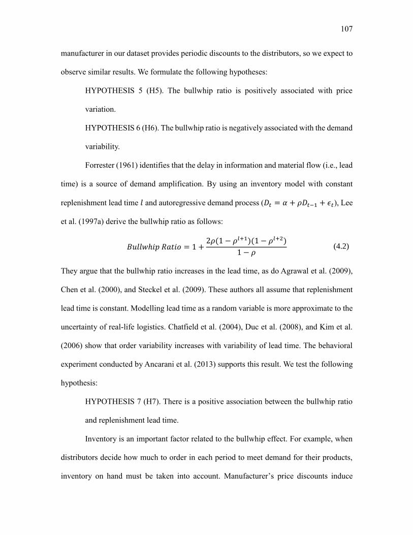
107
manufacturer in our dataset provides periodic discounts to the distributors, so we expect to
observe similar results. We formulate the following hypotheses:
HYPOTHESIS 5 (H5). The bullwhip ratio is positively associated with price
variation.
HYPOTHESIS 6 (H6). The bullwhip ratio is negatively associated with the demand
variability.
Forrester (1961) identifies that the delay in information and material flow (i.e., lead
time) is a source of demand amplification. By using an inventory model with constant
replenishment lead time 𝑙 and autoregressive demand process (𝐷𝑡 = 𝛼 + 𝜌𝐷𝑡−1 + 𝜖𝑡), Lee
et al. (1997a) derive the bullwhip ratio as follows:
𝐵𝑢𝑙𝑙𝑤ℎ𝑖𝑝 𝑅𝑎𝑡𝑖𝑜 = 1 +
2𝜌(1 − 𝜌𝑙+1)(1 − 𝜌𝑙+2)
1 − 𝜌 (4.2)
They argue that the bullwhip ratio increases in the lead time, as do Agrawal et al. (2009),
Chen et al. (2000), and Steckel et al. (2009). These authors all assume that replenishment
lead time is constant. Modelling lead time as a random variable is more approximate to the
uncertainty of real-life logistics. Chatfield et al. (2004), Duc et al. (2008), and Kim et al.
(2006) show that order variability increases with variability of lead time. The behavioral
experiment conducted by Ancarani et al. (2013) supports this result. We test the following
hypothesis:
HYPOTHESIS 7 (H7). There is a positive association between the bullwhip ratio
and replenishment lead time.
Inventory is an important factor related to the bullwhip effect. For example, when
distributors decide how much to order in each period to meet demand for their products,
inventory on hand must be taken into account. Manufacturer’s price discounts induce

108
distributors to forward buy and thus result in bullwhip effect. But a higher inventory level
causes distributors to order less to avoid additional holding cost, resulting in a lower
bullwhip effect. Experimental studies identify managers’ bounded rationality and sub-
optimal decisions as a behavioral cause of the bullwhip effect (e.g., Sterman, 1989; Croson
& Donohue, 2006). Over-reaction to demand changes is one of the managers’ errors in
decision making for inventory replenishment. Waston and Zheng (2008) show that
manager’s overreaction to demand signals can result in an increase in volatility of the
system’s replenishment orders. If a firm carries high inventory, the managers will be less
likely to place an inflated order when seeing a demand spike. Hence, inventory helps
mitigate the bullwhip effect. Baganha and Cohen (1998) develop an analytical model to
show that inventories can have a stabilizing effect on the replenishment orders. Bray and
Mendelson (2012) analytically illustrate that “the firm can reduce the bullwhip effect by
increasing product shelf life: a longer shelf life means a lower holding cost, which means
the firm carries a higher safety stock, which in turn means it reacts more calmly to demand
spikes” (p. 863). We use inventory to sales ratio (inventory ratio for short) to compare
inventory levels among SKUs and distributors. Our next hypothesis is as follows:
HYPOTHESIS 8 (H8). The inventory ratio is negatively associated with the
bullwhip ratio.
4.4 Empirical Context and Data
We use a proprietary dataset from a multiechelon pharmaceutical supply chain for
our empirical analysis. To the best of our knowledge, no prior empirical studies on the
bullwhip effect have the data at the same granularity level as ours. The dataset consists of

109
one manufacturer and six nation-wide distributors (A-F). The structure of the supply chain
and of the data is shown in Figure 4.1. This supply chain structure matches the one that is
widely used in theoretical studies on the bullwhip effect (e.g., Lee et al., 1997a; Cachon,
1999). The manufacturer produces consumable products that all medical practitioners in
this specialty use, and has a lion’s share of the market. These products are used on patients
in medical practitioners’ office and have a shelf life of approximately 18 months. In order
to meet sales targets, the manufacturer may periodically offer price discounts to its
distributors, for example, at the end of the manufacturer’s fiscal quarter.
We collect monthly data on 31 SKUs between January 2010 and June 2014. Since
the frequency of the data (monthly) matches the frequency of order decisions made by the
manufacturer and distributors, the data avoid the “time-disaggregation bias” identified by
Kahn (1992), and are suitable for appropriate supply chain cost assessment (Chen & Lee,
2012). The entire product category is made up of these 31 SKUs. SKUs 1-11 are carried by
all distributors. SKUs 12-15, 16-19, 20-23, 24-26, 27-28, and 29-31 are carried only by
distributors A-F, respectively. Manufacturer offers price discounts for 2 SKUs (SKUs 1 and
2), which account for 40% of the total sales. All 31 SKUs have annual wholesale price
increase. Specifically, we use the following data to conduct empirical analysis:
manufacturer’s production, manufacturer’s sales (distributors’ order receipts),
manufacturer’s raw material orders to the suppliers, manufacturer’s raw material receipts
from the suppliers, distributors’ orders (manufacturer’s demand), and distributors’ sales. In
general, sales is a censored variable and not the same as demand because it is equal to the
minimum of demand and inventory on hand. Both our interview with the industry expert
and public information from the distributors show that distributors’ sales almost exactly

110
match the orders from the practitioners. Hence, it is reasonable to assume for our dataset
that distributors’ sales are equivalent to their demand. Table 4.1 presents summary statistics
by distributor for the orders and sales variables used in our study. We do not have access
to the inventory data at distributors, so we estimate inventories using the following
relationship:
𝐼𝑛𝑣𝑒𝑛𝑡𝑜𝑟𝑦𝑡 = 𝐼𝑛𝑣𝑒𝑛𝑡𝑜𝑟𝑦𝑡−1 + 𝑂𝑟𝑑𝑒𝑟 𝑅𝑒𝑐𝑒𝑖𝑝𝑡𝑡 − 𝑆𝑎𝑙𝑒𝑠𝑡 (4.3)
where 𝐼𝑛𝑣𝑒𝑛𝑡𝑜𝑟𝑦𝑡 denotes the net inventories at the end of period 𝑡 . Since initial
inventories are not available, we choose them so that each period’s inventory is greater
than or equal to zero. Thus, the inventory data used in our analysis are relative inventory.
Similar approach has been used by Blattberg and Levin (1987). We measure quantities in
physical units rather than dollar amounts. This avoids measurement and accounting
problems associated with inventory evaluation (Lai, 2005). The Dickey-Fuller test suggests
that none of the data series presents a unit root, indicating that all data series are stationary.
Therefore, we do not make any adjustment to each series. Figure 4.2 shows sales and orders
of SKU 2 at distributor F. We observe that the distributor’s sales have much less variability
than its orders, indicating that the bullwhip effect exists. We notice that the distributor
places significant large orders during price discount periods and there is usually a trough
in orders after a price discount ends. This implies that the manufacturer’s price promotions
make the distributor’s orders more volatile than its sales and therefore leads to the bullwhip
effect.
4.5 Analysis
In Table 4.2, we report the bullwhip ratios at the SKU level. The substantial

111
bullwhip effect exists at each distributor. The average ratio is 22.88 (ranging from 1.13 to
216.67), much higher than those reported in the previous literature. Not all SKUs at
manufacturer exhibit the bullwhip effect, indicating that the manufacturer makes
production smoother than demand to some extent. The magnitude of the bullwhip ratios is
usually smaller at manufacturer than at distributors. The manufacturer (upstream firm) that
is supposed to suffer more from the bullwhip effect actually experiences a less severe
bullwhip effect than the distributors (downstream firm). Recall that manufacturer offers
price promotions for SKUs 1 and 2. The bullwhip ratios of these two SKUs at six
distributors are usually much larger than those of other SKUs, which implies that price
variation is a possible cause of the bullwhip effect. The interesting thing is that SKUs 1
and 2 at manufacturer have bullwhip ratios less than one. Our discussions with managers
of the manufacturer show that the factory operation prepares for the demand peaks caused
by the price promotions and is able to fulfill these demands from inventory in most cases.
Our findings at SKU level are similar to those obtained by Cachon et al. (2007) at industry
level.
Table 4.3 shows the bullwhip ratios measured by order variance and order receipt
variance for each SKU at distributors A-F. We find that the majority of SKUs at distributors
A, B, D, E, and F have a higher bullwhip ratio measured by order variance than that
measured by order receipt variance. Furthermore, paired t-tests (Table 4.4) show that
distributors A, B, D, and E have a statistically significantly higher bullwhip ratio measured
by variance of orders. We find strong evidence in support of H1. This result suggests that
the bullwhip measure based on material flow underestimates the one based on information
flow.
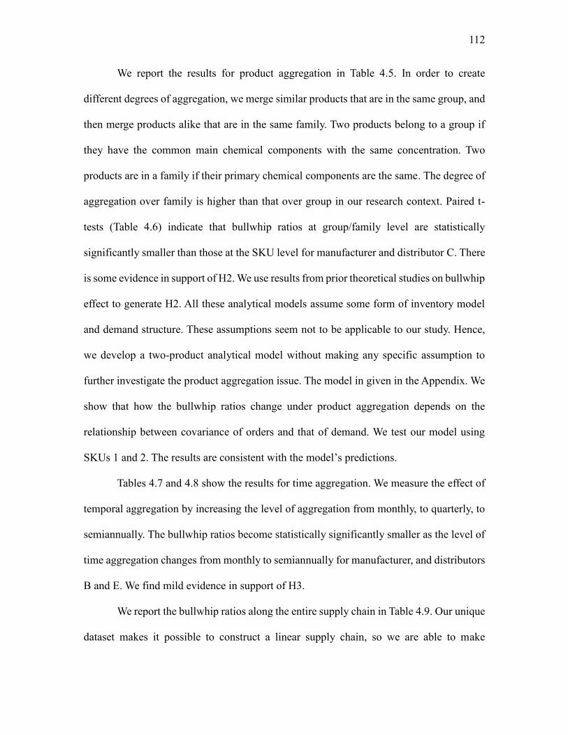
112
We report the results for product aggregation in Table 4.5. In order to create
different degrees of aggregation, we merge similar products that are in the same group, and
then merge products alike that are in the same family. Two products belong to a group if
they have the common main chemical components with the same concentration. Two
products are in a family if their primary chemical components are the same. The degree of
aggregation over family is higher than that over group in our research context. Paired t-
tests (Table 4.6) indicate that bullwhip ratios at group/family level are statistically
significantly smaller than those at the SKU level for manufacturer and distributor C. There
is some evidence in support of H2. We use results from prior theoretical studies on bullwhip
effect to generate H2. All these analytical models assume some form of inventory model
and demand structure. These assumptions seem not to be applicable to our study. Hence,
we develop a two-product analytical model without making any specific assumption to
further investigate the product aggregation issue. The model in given in the Appendix. We
show that how the bullwhip ratios change under product aggregation depends on the
relationship between covariance of orders and that of demand. We test our model using
SKUs 1 and 2. The results are consistent with the model’s predictions.
Tables 4.7 and 4.8 show the results for time aggregation. We measure the effect of
temporal aggregation by increasing the level of aggregation from monthly, to quarterly, to
semiannually. The bullwhip ratios become statistically significantly smaller as the level of
time aggregation changes from monthly to semiannually for manufacturer, and distributors
B and E. We find mild evidence in support of H3.
We report the bullwhip ratios along the entire supply chain in Table 4.9. Our unique
dataset makes it possible to construct a linear supply chain, so we are able to make
113
comparisons across different levels of the supply chain. The average bullwhip ratio is 28.59
(ranging from 0.13 to 132.17) for the entire supply chain, indicating that the bullwhip effect
is prevalent. The majority of 31 SKUs have bullwhip ratios greater than one at distributors
and manufacturer. T-test results show that manufacturer experiences a larger demand
variance than the distributors. Hence, H4 is supported.
To test hypotheses H5-H8, we develop the following econometric model:
𝐵𝑢𝑙𝑙𝑤ℎ𝑖𝑝𝑅𝑎𝑡𝑖𝑜𝑖𝑗 = 𝛽0 + 𝛽1𝑆𝐷𝑃𝑟𝑖𝑐𝑒𝑖𝑗 + 𝛽2𝐶𝑉𝐷𝑒𝑚𝑎𝑛𝑑𝑖𝑗 + 𝛽3𝐿𝑒𝑎𝑑𝑡𝑖𝑚𝑒𝑖𝑗
+ 𝛽4𝐼𝑅𝑖𝑗 + ∑ 𝛾𝑖𝐷𝑖𝑠𝑡𝑟𝑖𝑏𝑢𝑡𝑜𝑟𝑖
𝑖=𝐴,…,𝐸
+ 휀𝑖𝑗 (4.4)
Where 𝑖 denotes distributor, and 𝑗 denotes SKU. There are four explanatory variables with
each corresponding to a hypothesis. 𝑆𝐷𝑃𝑟𝑖𝑐𝑒 is the standard deviation of wholesale price.
In order to control for the range of price changes, we normalize the wholesale price using
the formula 𝑃𝑟𝑖𝑐𝑒𝑛𝑒𝑤 =𝑃𝑟𝑖𝑐𝑒−𝑃𝑟𝑖𝑐𝑒𝑚𝑖𝑛
𝑃𝑟𝑖𝑐𝑒𝑚𝑎𝑥−𝑃𝑟𝑖𝑐𝑒𝑚𝑖𝑛 . 𝐶𝑉𝐷𝑒𝑚𝑎𝑛𝑑 is the coefficient of variation of
demand. 𝐿𝑒𝑎𝑑𝑡𝑖𝑚𝑒 is the average number of days between placing an order and receiving
the ordered product. 𝐼𝑅 is the inventory ratio, which is calculated as the ratio of average
inventory to average sales. We include dummy variables 𝐷𝑖𝑠𝑡𝑟𝑖𝑏𝑢𝑡𝑜𝑟𝑖 to control for fixed
distributor effect. The variance inflation factor values for all explanatory variables are
between 1.43 and 2.26, which are lower than the cutoff value of 10 (Wooldridge, 2009).
Multicollinearity is not a problem. Estimation results are presented in Table 4.10.
The coefficient for 𝑆𝐷𝑃𝑟𝑖𝑐𝑒 is positive and significant, indicating that a greater
price variation is correlated with a higher bullwhip ratio. H5 is supported. This finding
provides empirical support to the analytical work by Lee et al. (1997a) and Sodhi et al.
(2014). The coefficient for 𝐶𝑉𝐷𝑒𝑚𝑎𝑛𝑑 is negative and significant, indicating that a higher

114
demand variability is correlated with a lower bullwhip ratio. We find strong evidence to
support H6. When demand becomes more predictable, the bullwhip effect is more likely to
occur. Table 4.11 shows the correlation coefficients between bullwhip ratio and coefficient
of variation of demand. All coefficients are negative and those for distributors D, E, and F
are statistically significant.
As shown in Table 4.10, the coefficient for 𝐿𝑒𝑎𝑑𝑡𝑖𝑚𝑒 is positive and significant.
This implies that a longer order lead time is associated with a higher bullwhip ratio. We
find strong evidence in support of H7. Table 4.12 shows the correlation coefficients
between replenishment lead time and bullwhip ratio. We find that there is a positive
association between bullwhip ratio and lead time for distributor A, B, D, and E. The
coefficient for 𝐼𝑅 is negative and significant, indicating that a higher inventory is correlated
with a lower bullwhip ratio. H8 is supported. We report the correlation coefficients between
inventory ratio and bullwhip ratio for distributors in Table 4.13. We find that there is a
statistically significantly negative association between inventory ratio and bullwhip ratio
for distributors A, D, and F, and there is a negative but not significant relationship for
distributor E.
A firm will not exhibit a bullwhip effect if it operates in a perfectly-matched fashion.
That is, the firm’s shipment (i.e., sales to customers) stream coincides with the demand
(i.e., orders received from the customers) stream; the shipments come directly out of a just-
in-time manufacturing stream, indicating that there is no need to hold finished goods
inventory; the firm places raw material orders with its supplier by exactly following the
manufacturing stream, and the supplier fulfills these orders instantaneously, resulting in no
raw material inventory. If each firm along a supply chain uses the perfectly-matched

115
strategy, the entire chain will not exhibit a bullwhip effect.
However, we find not only prevalent but also intensive bullwhip effects in our
dataset. To better understand the bullwhip effect in a firm and along the supply chain, we
break down the inter-firm bullwhip ratio into individual intra-firm bullwhips by following
the bullwhip effect decomposition framework developed in Chapter 3. This decomposition
helps one think about the relationships between various information and material flows that
are involved in a firm’s decision-making process. Figure 4.3 illustrates the framework in a
two-echelon supply chain: a distributor (downstream) and a manufacturer (upstream). The
distributor and the manufacturer are denoted as firms D and U, respectively. We organize
our discussion around the manufacturer. Similar discussion is applicable to the distributor.
Firm U receives a demand stream (orders from distributor) with variance 𝑉𝐷𝑈 (the
superscript refers to firm U, and the subscript D denotes that this is the variance of the
demand stream). Due to constraints in manufacturing and inventory, firm U may not be
able to fulfill demands immediately, so its shipment stream may not exactly match its
demand stream. For example, the anticipation of economic boom causes customers to place
orders too large to be filled instantly via inventory on hand and/or current manufacturing
output. Thus, the variance of firm U’s shipment stream denoted by 𝑉𝑆𝑈 (the superscript
denotes firm U and the subscript S refer to the shipment) may differ from the variance of
its demand stream. We define firm U’s shipment bullwhip as the variance ratio 𝑉𝑆
𝑈
𝑉𝐷𝑈, and
denote this bullwhip ratio by 𝐵𝑆𝑈. That is, 𝐵𝑆
𝑈 =𝑉𝑆
𝑈
𝑉𝐷𝑈. The shipment bullwhip indicates an
amplification of the demand stream when 𝐵𝑆𝑈 > 1 and a smoothing of the demand stream
when 𝐵𝑆𝑈 < 1.
116
Firm U’s manufacturing stream will not necessarily match its shipment stream due
to various factors such as seasonal demand, convex manufacturing cost function, and batch
manufacturing. For example, suppose firm U faces seasonal demand throughout the year.
Then the firm may find that it is appropriate to smooth its manufacturing relative to its
shipment by using finished goods inventory as a buffer with the following results: Produce
at relatively stable rate, build inventory during periods of low demand, and draw down
inventory in periods of high demand. In order to recognize the fact that the manufacturing
stream may differ from the shipment stream, we define manufacturing bullwhip as 𝐵𝑀𝑈 =
𝑉𝑀𝑈
𝑉𝑆𝑈 , where 𝑉𝑀
𝑈 denotes the variance in the manufacturing stream. The manufacturing
bullwhip may indicate an amplification (𝐵𝑀𝑈 > 1) or a smoothing (𝐵𝑀
𝑈 < 1).
Similarly, firm U may find that it is not optimal to order raw materials to exactly
follow its manufacturing stream due to sales promotion, demand uncertainty, and order
batching. For example, the firm’s supplier may offer periodic discounts to boost sales or
liquidate material surpluses. The firm can forward buy and hold raw material inventory to
save purchase cost, resulting in a volatile order stream compared to manufacturing stream.
To capture the discrepancy between order and manufacturing stream, we define the order
bullwhip as 𝐵𝑂𝑈 =
𝑉𝑂𝑈
𝑉𝑀𝑈, where 𝑉𝑂
𝑈 denotes the variance in stream of orders that firm U places.
Again, the order bullwhip may indicate an amplification (𝐵𝑂𝑈 > 1) or a smoothing (𝐵𝑂
𝑈 <
1 ). For firm D (distributor) that performs no manufacturing, there is no intermediate
manufacturing stream between the order stream and the shipment stream. So the order
bullwhip becomes 𝐵𝑂𝐷 =
𝑉𝑂𝐷
𝑉𝑆𝐷.
The information-based full bullwhip ratio, which we denote by 𝐵𝑈, is defined as

117
𝐵𝑈 =𝑉𝑂
𝑈
𝑉𝐷𝑈. We can write firm U’s full bullwhip ratio as the multiplicative effect of three
intra-firm component bullwhips, namely shipment bullwhip, manufacturing bullwhip, and
order bullwhip:
𝐵𝑈 =
𝑉𝑂𝑈
𝑉𝐷𝑈 = (
𝑉𝑆𝑈
𝑉𝐷𝑈) (
𝑉𝑀𝑈
𝑉𝑆𝑈) (
𝑉𝑂𝑈
𝑉𝑀𝑈) = 𝐵𝑆
𝑈 ∗ 𝐵𝑀𝑈 ∗ 𝐵𝑂
𝑈 (4.5)
Due to data availability issues, some previous studies use a surrogate measure to estimate
the bullwhip ratio 𝐵𝑈. For example, Cachon et al. (2007) do not have access to the orders
and therefore use what they call “production” as a proxy for these orders, which is
calculated as sales plus the change in inventory (i.e., the difference between ending and
beginning inventory). This production stream represents the inflow of materials (i.e., order
receipt). For a firm (such as a wholesaler) that performs no manufacturing, the production
stream is directly equivalent to the inflow of finished goods. Since “production” may have
various connotations, we will use the term “inflow” (order receipt) to represent the
production stream and denote the inflow variance by 𝑉𝐼𝑈. We define the inflow bullwhip as
𝐵𝐼𝑈 =
𝑉𝐼𝑈
𝑉𝑂𝑈 . Note that firm D’s inflow stream is actually shipment stream of firm U, so
variance of firm D’s inflow stream (𝑉𝐼𝐷) is equal to variance of firm U’s shipment stream
(𝑉𝑆𝑈). Also note that U’s demand stream is equal to D’s order stream, which implies that
𝑉𝑂𝐷 = 𝑉𝐷
𝑈. The measure 𝐵∗𝑈 =
𝑉𝐼𝑈
𝑉𝐷𝑈 is then used as a surrogate for the bullwhip ratio 𝐵𝑈 (we
put an asterisk in the subscript to denote that it is a surrogate measure). Note that 𝐵∗𝑈 =
𝑉𝐼𝑈
𝑉𝐷𝐷 = 𝐵𝑆
𝑈 ∗ 𝐵𝑀𝑈 ∗ 𝐵𝑂
𝑈 ∗ 𝐵𝐼𝑈 . That is, the proxy bullwhip ratio 𝐵∗
𝑈 is equal to the bullwhip
ratio 𝐵𝑈 multiplied by the inflow bullwhip. Bray and Mendelson (2012) and Shan et al.
(2014) use sales and production (which we call inflow) as proxy variables for demand and

118
orders, respectively. These authors calculate the material-based bullwhip ratio as 𝐵∗∗𝑈 =
𝑉𝐼𝑈
𝑉𝑆𝑈 = 𝐵𝑀
𝑈 ∗ 𝐵𝑂𝑈 ∗ 𝐵𝐼
𝑈 (we use double asterisk in the subscript to denote this bullwhip ratio).
The above decomposition allows us to consider the bullwhip effect by looking at
its individual components. For the distributors in our dataset, the shipment stream (i.e.,
sales to customers) is almost equivalent to the demand stream, indicating that 𝐵𝑆𝐷 = 1. As
we mentioned before, distributors do not perform manufacturing, so there is no
manufacturing bullwhip and the order bullwhip becomes 𝐵𝑂𝐷 =
𝑉𝑂𝐷
𝑉𝑆𝐷 . In short, the full
bullwhip ( 𝐵∗𝐷 ) of a distributor can be written as 𝐵∗
𝐷 = 𝐵𝑂𝐷 ∗ 𝐵𝐼
𝐷 . Table 4.14 shows
distributors’ individual intra-firm bullwhips. We find that the majority of SKUs at
distributors A, B, D, and E have a smoother inflow stream compared to the order stream
(𝐵𝐼𝐷 < 1 ). This implies that manufacturer smooths shipment stream relative to demand
stream, resulting in a dampening effect on the distributor’s full bullwhip. Conversely, most
SKUs at distributor C and about half SKUs at distributor F have an amplifying inflow
stream compared to order stream ( 𝐵𝐼𝐷 > 1 ), indicating that manufacturer’s shipment
bullwhip amplifies the distributor’s full bullwhip. Manufacturer’s individual intra-firm
bullwhips are shown in Table 4.15. We find that manufacturer’s shipment stream is
smoother than its demand stream (𝐵𝑆𝑈 < 1) and its manufacturing stream is more volatile
that its shipment stream (𝐵𝑀𝑈 > 1). Our interview with managers of the manufacturer helps
explain why the firm exhibits such behaviors: 1) When manufacturer offers distributors
price discounts, the distributors sometimes place a significant large order. So manufacturer
will not be able to fulfill orders immediately and have to spread out shipments in the next
few months. This makes shipment stream smoother that demand stream. 2) The firm uses

119
batch manufacturing due to economy of scale, resulting in a more variable manufacturing
stream compared to the shipment stream.
Each SKU contains only one main chemical component and there are a total of four
main chemical components in our dataset. We denote these components by chemicals A,
B, L, and M and calculate individual bullwhips for each chemical. The results are shown
in Table 4.16. Since we are not able to keep track of the raw chemical material usage in the
actual manufacturing process, we use imputed manufacturing (raw material receipt plus
change in raw material inventory) for the order bullwhip. Distributors’ order bullwhip is
greater than one for each chemical. This suggests that distributors amplify demand
variability. All chemicals at manufacturer have shipment bullwhip less than one, indicating
that the manufacturer smooths shipment relative to demand. Manufacturer’s order bullwhip
is greater than one for each chemical. This implies that the manufacturer amplifies orders
placed to its supplier relative to its manufacturing output. The manufacturing bullwhip is
positively correlated with the shipment bullwhip and negatively correlated with the order
bullwhip. The inflow bullwhip is negatively correlated with the order bullwhip.
4.6 Conclusion
The bullwhip effect is one of the central observations in economics and operations
management and has drawn much attention from both academia and industry. There has
been an extensive literature of theoretical studies on the bullwhip effect, but empirical
studies are still limited due to data availability issues. By using a unique dataset from a
multiechelon pharmaceutical supply chain, we are able to address several empirical
challenges identified in the prior literature and make a contribution to the literature. In
120
particular, we investigate the existence and magnitude of the bullwhip effect at SKU level,
analyze the impact of data aggregation on the bullwhip measurement, and test a number of
driving factors of the bullwhip effect.
We find that the bullwhip effect at SKU level is prevalent and intensive at
distributors. Manufacturer (upstream) exhibits a less intensive bullwhip effect than
distributors (downstream). The manufacturer does not suffer as much as we previously
thought. But we do observe that the manufacturer has greater demand variance than the
distributors. We find that the bullwhip ratio based on order variance is higher than that
based on order receipt variance. The material-based bullwhip measure that is widely used
in prior empirical studies underestimates the information-based measure. We observe that
product aggregation and time aggregation tend to mask the bullwhip effect in some cases.
We find that SKUs that have more predictable demands are more likely to exhibit the
bullwhip effect. Manufacturer smooths production relative to demand for several SKUs,
providing empirical support to production smoothing hypothesis. We find that most
prominent factors related to the bullwhip effect are price variation, order lead time, and
inventory.
Our study has some limitations. First, our data are from a single supply chain and
for pharmaceutical products. This limits the generalizability of our findings to other
industries and other types of products. We advocate caution in out-of-sample inferences.
Second, similar to other empirical research, our study is only able to estimate associations
rather than test for causality.
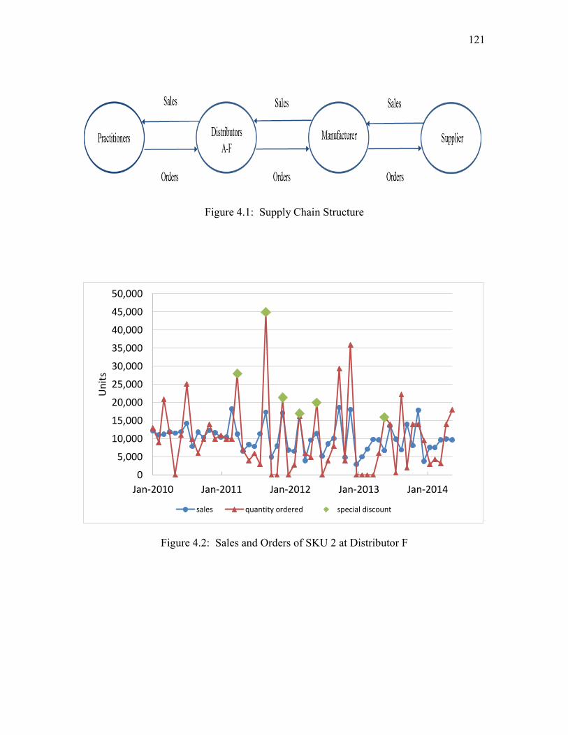
121
Figure 4.1: Supply Chain Structure
Figure 4.2: Sales and Orders of SKU 2 at Distributor F
0
5,000
10,000
15,000
20,000
25,000
30,000
35,000
40,000
45,000
50,000
Jan-2010 Jan-2011 Jan-2012 Jan-2013 Jan-2014
Un
its
sales quantity ordered special discount
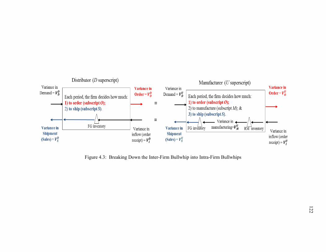
122
Figure 4.3: Breaking Down the Inter-Firm Bullwhip into Intra-Firm Bullwhips
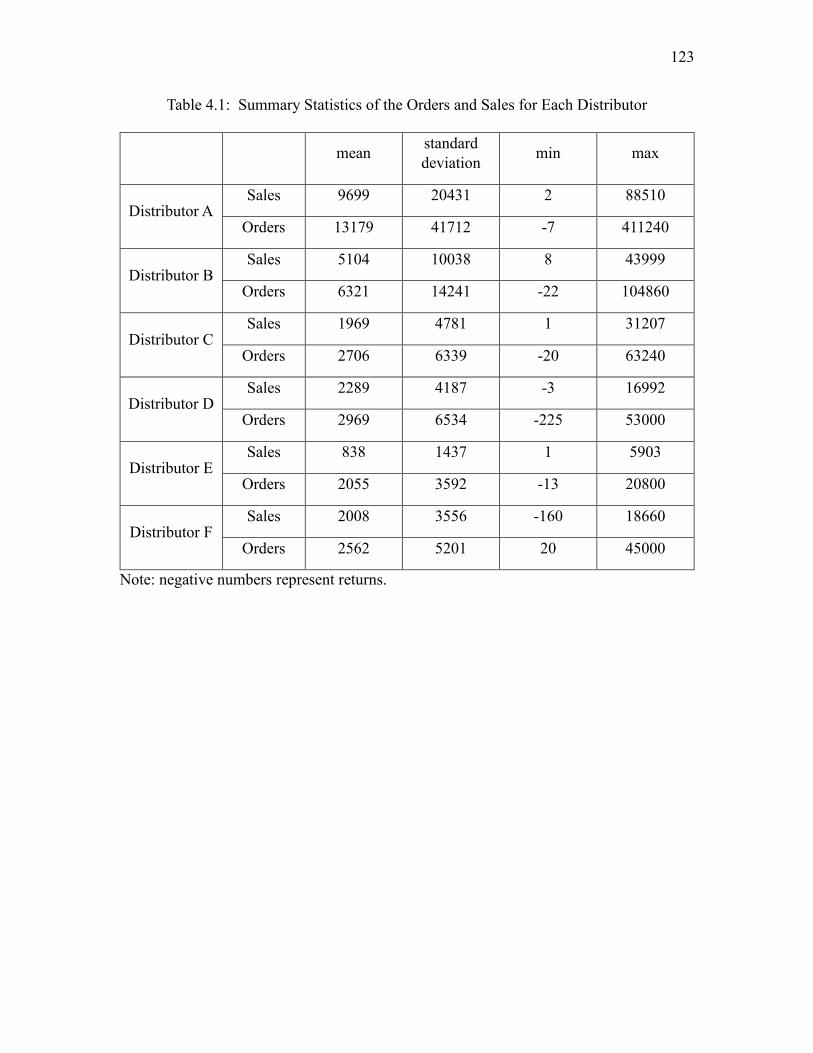
123
Table 4.1: Summary Statistics of the Orders and Sales for Each Distributor
mean standard
deviation min max
Distributor A Sales 9699 20431 2 88510
Orders 13179 41712 -7 411240
Distributor B Sales 5104 10038 8 43999
Orders 6321 14241 -22 104860
Distributor C Sales 1969 4781 1 31207
Orders 2706 6339 -20 63240
Distributor D Sales 2289 4187 -3 16992
Orders 2969 6534 -225 53000
Distributor E Sales 838 1437 1 5903
Orders 2055 3592 -13 20800
Distributor F Sales 2008 3556 -160 18660
Orders 2562 5201 20 45000
Note: negative numbers represent returns.
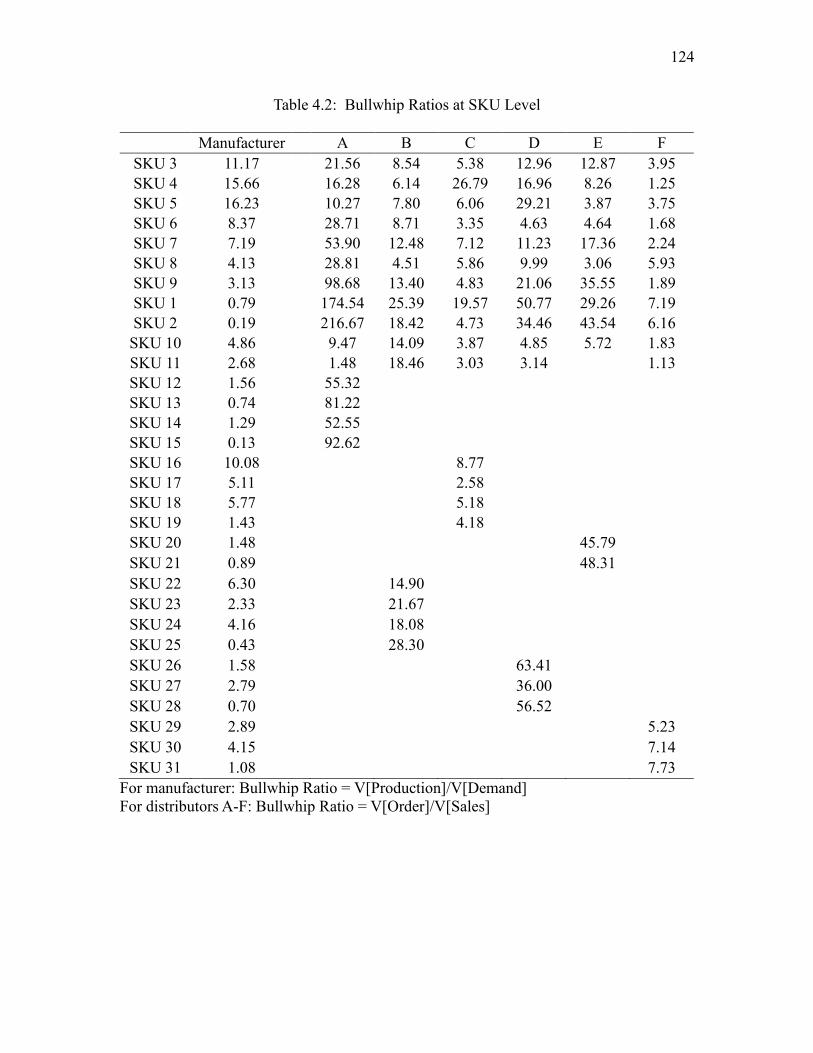
124
Table 4.2: Bullwhip Ratios at SKU Level
Manufacturer A B C D E F
SKU 3 11.17 21.56 8.54 5.38 12.96 12.87 3.95
SKU 4 15.66 16.28 6.14 26.79 16.96 8.26 1.25
SKU 5 16.23 10.27 7.80 6.06 29.21 3.87 3.75
SKU 6 8.37 28.71 8.71 3.35 4.63 4.64 1.68
SKU 7 7.19 53.90 12.48 7.12 11.23 17.36 2.24
SKU 8 4.13 28.81 4.51 5.86 9.99 3.06 5.93
SKU 9 3.13 98.68 13.40 4.83 21.06 35.55 1.89
SKU 1 0.79 174.54 25.39 19.57 50.77 29.26 7.19
SKU 2 0.19 216.67 18.42 4.73 34.46 43.54 6.16
SKU 10 4.86 9.47 14.09 3.87 4.85 5.72 1.83
SKU 11 2.68 1.48 18.46 3.03 3.14 1.13
SKU 12 1.56 55.32
SKU 13 0.74 81.22
SKU 14 1.29 52.55
SKU 15 0.13 92.62
SKU 16 10.08 8.77
SKU 17 5.11 2.58
SKU 18 5.77 5.18
SKU 19 1.43 4.18
SKU 20 1.48 45.79
SKU 21 0.89 48.31
SKU 22 6.30 14.90
SKU 23 2.33 21.67
SKU 24 4.16 18.08
SKU 25 0.43 28.30
SKU 26 1.58 63.41
SKU 27 2.79 36.00
SKU 28 0.70 56.52
SKU 29 2.89 5.23
SKU 30 4.15 7.14
SKU 31 1.08 7.73
For manufacturer: Bullwhip Ratio = V[Production]/V[Demand]
For distributors A-F: Bullwhip Ratio = V[Order]/V[Sales]
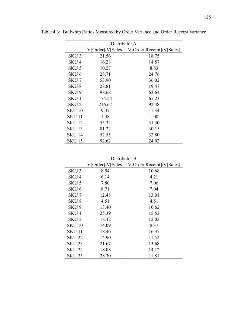
125
Table 4.3: Bullwhip Ratios Measured by Order Variance and Order Receipt Variance
Distributor A
V[Order]/V[Sales] V[Order Receipt]/V[Sales]
SKU 3 21.56 18.75
SKU 4 16.28 14.57
SKU 5 10.27 8.83
SKU 6 28.71 24.76
SKU 7 53.90 36.02
SKU 8 28.81 19.47
SKU 9 98.68 63.64
SKU 1 174.54 67.23
SKU 2 216.67 92.48
SKU 10 9.47 11.34
SKU 11 1.48 1.00
SKU 12 55.32 31.30
SKU 13 81.22 30.15
SKU 14 52.55 32.80
SKU 15 92.62 24.02
Distributor B
V[Order]/V[Sales] V[Order Receipt]/V[Sales]
SKU 3 8.54 10.68
SKU 4 6.14 4.21
SKU 5 7.80 7.06
SKU 6 8.71 7.04
SKU 7 12.48 13.01
SKU 8 4.51 4.51
SKU 9 13.40 10.62
SKU 1 25.39 15.52
SKU 2 18.42 12.02
SKU 10 14.09 8.37
SKU 11 18.46 16.37
SKU 22 14.90 11.52
SKU 23 21.67 13.68
SKU 24 18.08 14.12
SKU 25 28.30 11.81
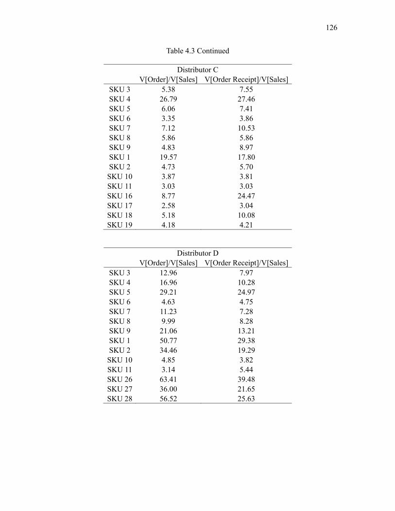
126
Table 4.3 Continued
Distributor C
V[Order]/V[Sales] V[Order Receipt]/V[Sales]
SKU 3 5.38 7.55
SKU 4 26.79 27.46
SKU 5 6.06 7.41
SKU 6 3.35 3.86
SKU 7 7.12 10.53
SKU 8 5.86 5.86
SKU 9 4.83 8.97
SKU 1 19.57 17.80
SKU 2 4.73 5.70
SKU 10 3.87 3.81
SKU 11 3.03 3.03
SKU 16 8.77 24.47
SKU 17 2.58 3.04
SKU 18 5.18 10.08
SKU 19 4.18 4.21
Distributor D
V[Order]/V[Sales] V[Order Receipt]/V[Sales]
SKU 3 12.96 7.97
SKU 4 16.96 10.28
SKU 5 29.21 24.97
SKU 6 4.63 4.75
SKU 7 11.23 7.28
SKU 8 9.99 8.28
SKU 9 21.06 13.21
SKU 1 50.77 29.38
SKU 2 34.46 19.29
SKU 10 4.85 3.82
SKU 11 3.14 5.44
SKU 26 63.41 39.48
SKU 27 36.00 21.65
SKU 28 56.52 25.63
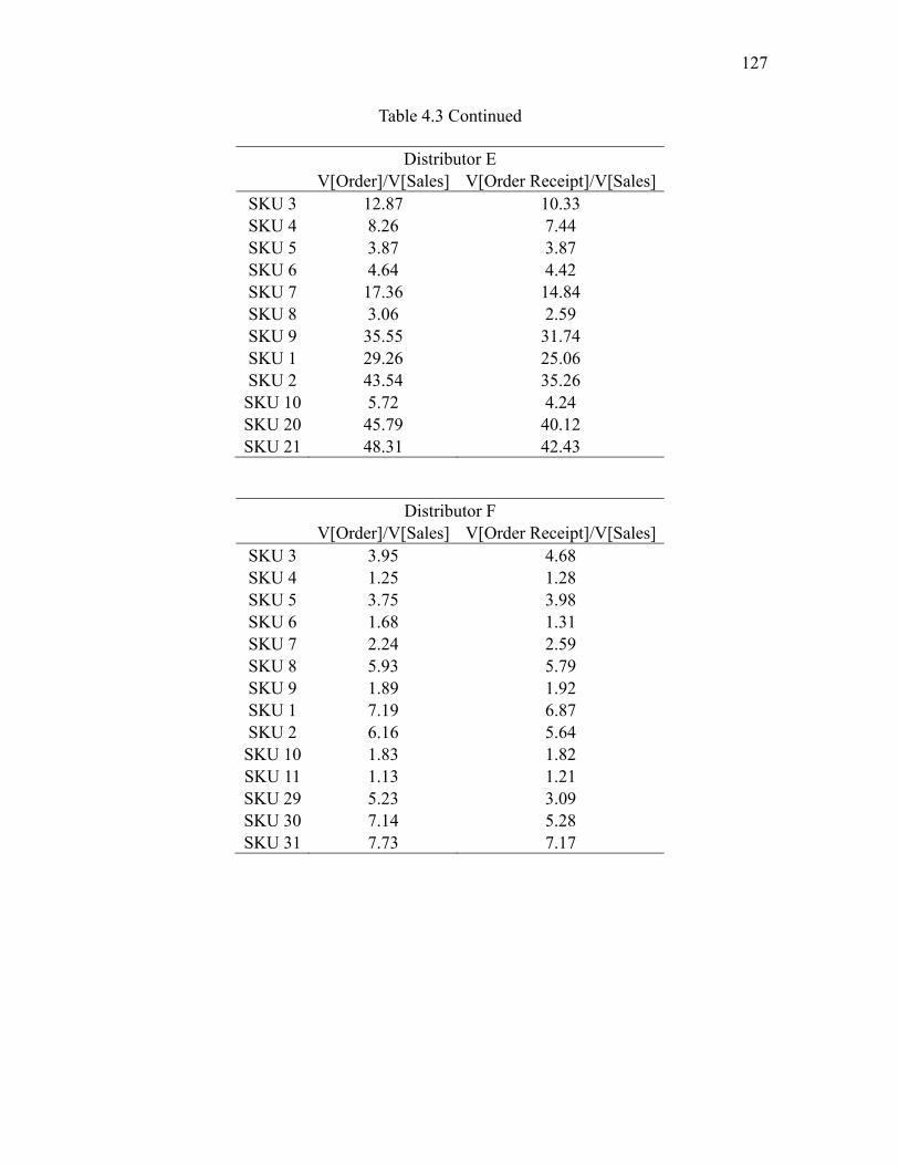
127
Table 4.3 Continued
Distributor E
V[Order]/V[Sales] V[Order Receipt]/V[Sales]
SKU 3 12.87 10.33
SKU 4 8.26 7.44
SKU 5 3.87 3.87
SKU 6 4.64 4.42
SKU 7 17.36 14.84
SKU 8 3.06 2.59
SKU 9 35.55 31.74
SKU 1 29.26 25.06
SKU 2 43.54 35.26
SKU 10 5.72 4.24
SKU 20 45.79 40.12
SKU 21 48.31 42.43
Distributor F
V[Order]/V[Sales] V[Order Receipt]/V[Sales]
SKU 3 3.95 4.68
SKU 4 1.25 1.28
SKU 5 3.75 3.98
SKU 6 1.68 1.31
SKU 7 2.24 2.59
SKU 8 5.93 5.79
SKU 9 1.89 1.92
SKU 1 7.19 6.87
SKU 2 6.16 5.64
SKU 10 1.83 1.82
SKU 11 1.13 1.21
SKU 29 5.23 3.09
SKU 30 7.14 5.28
SKU 31 7.73 7.17
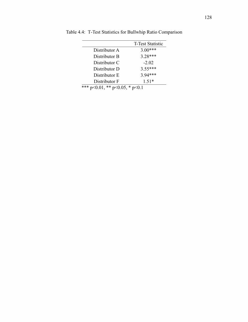
128
Table 4.4: T-Test Statistics for Bullwhip Ratio Comparison
T-Test Statistic
Distributor A 3.00***
Distributor B 3.28***
Distributor C -2.02
Distributor D 3.55***
Distributor E 3.94***
Distributor F 1.51*
*** p<0.01, ** p<0.05, * p<0.1
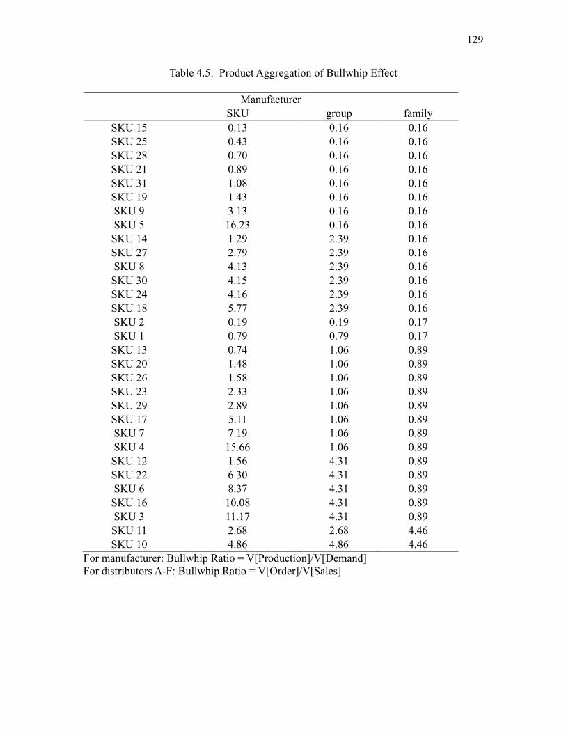
129
Table 4.5: Product Aggregation of Bullwhip Effect
Manufacturer
SKU group family
SKU 15 0.13 0.16 0.16
SKU 25 0.43 0.16 0.16
SKU 28 0.70 0.16 0.16
SKU 21 0.89 0.16 0.16
SKU 31 1.08 0.16 0.16
SKU 19 1.43 0.16 0.16
SKU 9 3.13 0.16 0.16
SKU 5 16.23 0.16 0.16
SKU 14 1.29 2.39 0.16
SKU 27 2.79 2.39 0.16
SKU 8 4.13 2.39 0.16
SKU 30 4.15 2.39 0.16
SKU 24 4.16 2.39 0.16
SKU 18 5.77 2.39 0.16
SKU 2 0.19 0.19 0.17
SKU 1 0.79 0.79 0.17
SKU 13 0.74 1.06 0.89
SKU 20 1.48 1.06 0.89
SKU 26 1.58 1.06 0.89
SKU 23 2.33 1.06 0.89
SKU 29 2.89 1.06 0.89
SKU 17 5.11 1.06 0.89
SKU 7 7.19 1.06 0.89
SKU 4 15.66 1.06 0.89
SKU 12 1.56 4.31 0.89
SKU 22 6.30 4.31 0.89
SKU 6 8.37 4.31 0.89
SKU 16 10.08 4.31 0.89
SKU 3 11.17 4.31 0.89
SKU 11 2.68 2.68 4.46
SKU 10 4.86 4.86 4.46
For manufacturer: Bullwhip Ratio = V[Production]/V[Demand]
For distributors A-F: Bullwhip Ratio = V[Order]/V[Sales]
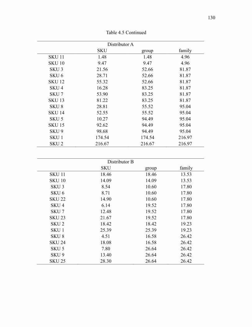
130
Table 4.5 Continued
Distributor A
SKU group family
SKU 11 1.48 1.48 4.96
SKU 10 9.47 9.47 4.96
SKU 3 21.56 52.66 81.87
SKU 6 28.71 52.66 81.87
SKU 12 55.32 52.66 81.87
SKU 4 16.28 83.25 81.87
SKU 7 53.90 83.25 81.87
SKU 13 81.22 83.25 81.87
SKU 8 28.81 55.52 95.04
SKU 14 52.55 55.52 95.04
SKU 5 10.27 94.49 95.04
SKU 15 92.62 94.49 95.04
SKU 9 98.68 94.49 95.04
SKU 1 174.54 174.54 216.97
SKU 2 216.67 216.67 216.97
Distributor B
SKU group family
SKU 11 18.46 18.46 13.53
SKU 10 14.09 14.09 13.53
SKU 3 8.54 10.60 17.80
SKU 6 8.71 10.60 17.80
SKU 22 14.90 10.60 17.80
SKU 4 6.14 19.52 17.80
SKU 7 12.48 19.52 17.80
SKU 23 21.67 19.52 17.80
SKU 2 18.42 18.42 19.23
SKU 1 25.39 25.39 19.23
SKU 8 4.51 16.58 26.42
SKU 24 18.08 16.58 26.42
SKU 5 7.80 26.64 26.42
SKU 9 13.40 26.64 26.42
SKU 25 28.30 26.64 26.42
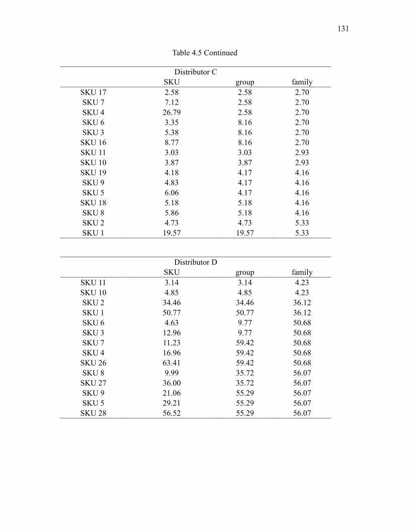
131
Table 4.5 Continued
Distributor C
SKU group family
SKU 17 2.58 2.58 2.70
SKU 7 7.12 2.58 2.70
SKU 4 26.79 2.58 2.70
SKU 6 3.35 8.16 2.70
SKU 3 5.38 8.16 2.70
SKU 16 8.77 8.16 2.70
SKU 11 3.03 3.03 2.93
SKU 10 3.87 3.87 2.93
SKU 19 4.18 4.17 4.16
SKU 9 4.83 4.17 4.16
SKU 5 6.06 4.17 4.16
SKU 18 5.18 5.18 4.16
SKU 8 5.86 5.18 4.16
SKU 2 4.73 4.73 5.33
SKU 1 19.57 19.57 5.33
Distributor D
SKU group family
SKU 11 3.14 3.14 4.23
SKU 10 4.85 4.85 4.23
SKU 2 34.46 34.46 36.12
SKU 1 50.77 50.77 36.12
SKU 6 4.63 9.77 50.68
SKU 3 12.96 9.77 50.68
SKU 7 11.23 59.42 50.68
SKU 4 16.96 59.42 50.68
SKU 26 63.41 59.42 50.68
SKU 8 9.99 35.72 56.07
SKU 27 36.00 35.72 56.07
SKU 9 21.06 55.29 56.07
SKU 5 29.21 55.29 56.07
SKU 28 56.52 55.29 56.07
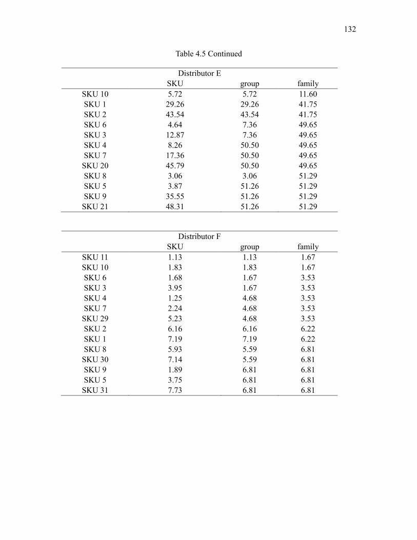
132
Table 4.5 Continued
Distributor E
SKU group family
SKU 10 5.72 5.72 11.60
SKU 1 29.26 29.26 41.75
SKU 2 43.54 43.54 41.75
SKU 6 4.64 7.36 49.65
SKU 3 12.87 7.36 49.65
SKU 4 8.26 50.50 49.65
SKU 7 17.36 50.50 49.65
SKU 20 45.79 50.50 49.65
SKU 8 3.06 3.06 51.29
SKU 5 3.87 51.26 51.29
SKU 9 35.55 51.26 51.29
SKU 21 48.31 51.26 51.29
Distributor F
SKU group family
SKU 11 1.13 1.13 1.67
SKU 10 1.83 1.83 1.67
SKU 6 1.68 1.67 3.53
SKU 3 3.95 1.67 3.53
SKU 4 1.25 4.68 3.53
SKU 7 2.24 4.68 3.53
SKU 29 5.23 4.68 3.53
SKU 2 6.16 6.16 6.22
SKU 1 7.19 7.19 6.22
SKU 8 5.93 5.59 6.81
SKU 30 7.14 5.59 6.81
SKU 9 1.89 6.81 6.81
SKU 5 3.75 6.81 6.81
SKU 31 7.73 6.81 6.81
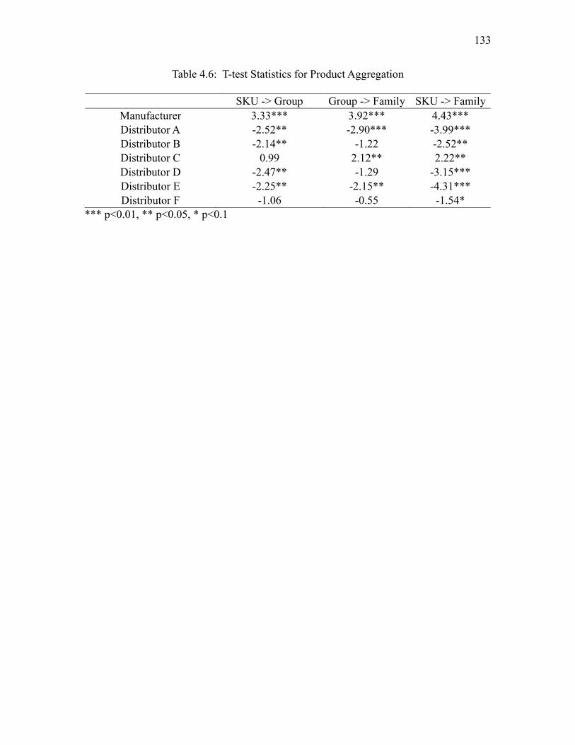
133
Table 4.6: T-test Statistics for Product Aggregation
SKU -> Group Group -> Family SKU -> Family
Manufacturer 3.33*** 3.92*** 4.43***
Distributor A -2.52** -2.90*** -3.99***
Distributor B -2.14** -1.22 -2.52**
Distributor C 0.99 2.12** 2.22**
Distributor D -2.47** -1.29 -3.15***
Distributor E -2.25** -2.15** -4.31***
Distributor F -1.06 -0.55 -1.54*
*** p<0.01, ** p<0.05, * p<0.1
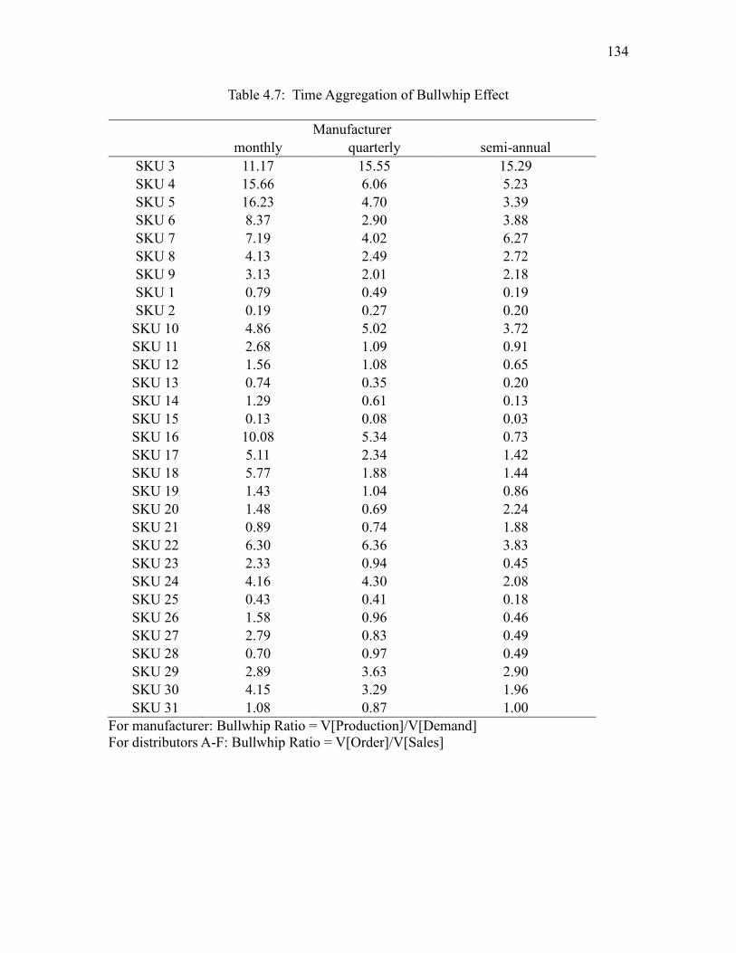
134
Table 4.7: Time Aggregation of Bullwhip Effect
Manufacturer
monthly quarterly semi-annual
SKU 3 11.17 15.55 15.29
SKU 4 15.66 6.06 5.23
SKU 5 16.23 4.70 3.39
SKU 6 8.37 2.90 3.88
SKU 7 7.19 4.02 6.27
SKU 8 4.13 2.49 2.72
SKU 9 3.13 2.01 2.18
SKU 1 0.79 0.49 0.19
SKU 2 0.19 0.27 0.20
SKU 10 4.86 5.02 3.72
SKU 11 2.68 1.09 0.91
SKU 12 1.56 1.08 0.65
SKU 13 0.74 0.35 0.20
SKU 14 1.29 0.61 0.13
SKU 15 0.13 0.08 0.03
SKU 16 10.08 5.34 0.73
SKU 17 5.11 2.34 1.42
SKU 18 5.77 1.88 1.44
SKU 19 1.43 1.04 0.86
SKU 20 1.48 0.69 2.24
SKU 21 0.89 0.74 1.88
SKU 22 6.30 6.36 3.83
SKU 23 2.33 0.94 0.45
SKU 24 4.16 4.30 2.08
SKU 25 0.43 0.41 0.18
SKU 26 1.58 0.96 0.46
SKU 27 2.79 0.83 0.49
SKU 28 0.70 0.97 0.49
SKU 29 2.89 3.63 2.90
SKU 30 4.15 3.29 1.96
SKU 31 1.08 0.87 1.00
For manufacturer: Bullwhip Ratio = V[Production]/V[Demand]
For distributors A-F: Bullwhip Ratio = V[Order]/V[Sales]
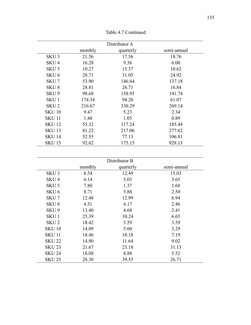
135
Table 4.7 Continued
Distributor A
monthly quarterly semi-annual
SKU 3 21.56 17.56 18.76
SKU 4 16.28 9.36 6.00
SKU 5 10.27 15.37 10.62
SKU 6 28.71 31.05 24.92
SKU 7 53.90 146.64 137.18
SKU 8 28.81 26.71 16.84
SKU 9 98.68 158.95 141.74
SKU 1 174.54 94.20 61.07
SKU 2 216.67 330.29 269.14
SKU 10 9.47 5.23 2.34
SKU 11 1.48 1.05 0.89
SKU 12 55.32 117.24 185.44
SKU 13 81.22 217.06 277.62
SKU 14 52.55 77.13 106.81
SKU 15 92.62 175.15 928.13
Distributor B
monthly quarterly semi-annual
SKU 3 8.54 12.49 15.03
SKU 4 6.14 5.03 3.65
SKU 5 7.80 1.37 1.68
SKU 6 8.71 5.88 2.50
SKU 7 12.48 12.99 6.94
SKU 8 4.51 4.17 2.46
SKU 9 13.40 4.68 2.41
SKU 1 25.39 10.24 6.65
SKU 2 18.42 5.59 3.59
SKU 10 14.09 5.60 3.29
SKU 11 18.46 10.18 7.19
SKU 22 14.90 11.64 9.02
SKU 23 21.67 23.18 31.13
SKU 24 18.08 8.88 5.52
SKU 25 28.30 39.55 26.71
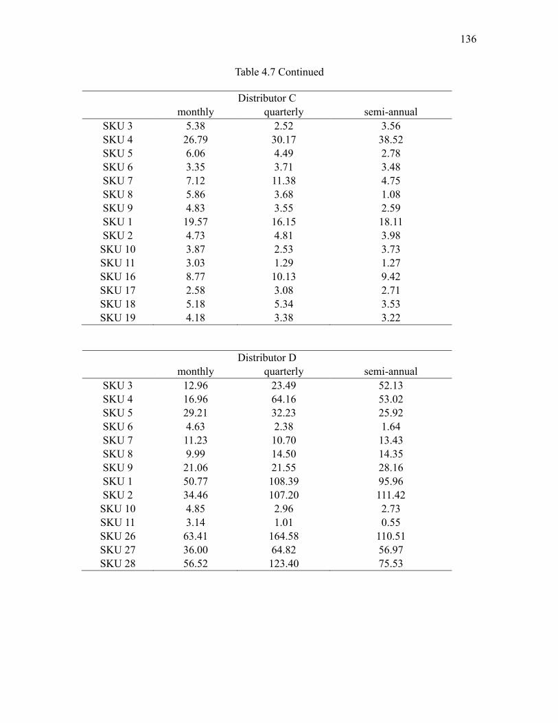
136
Table 4.7 Continued
Distributor C
monthly quarterly semi-annual
SKU 3 5.38 2.52 3.56
SKU 4 26.79 30.17 38.52
SKU 5 6.06 4.49 2.78
SKU 6 3.35 3.71 3.48
SKU 7 7.12 11.38 4.75
SKU 8 5.86 3.68 1.08
SKU 9 4.83 3.55 2.59
SKU 1 19.57 16.15 18.11
SKU 2 4.73 4.81 3.98
SKU 10 3.87 2.53 3.73
SKU 11 3.03 1.29 1.27
SKU 16 8.77 10.13 9.42
SKU 17 2.58 3.08 2.71
SKU 18 5.18 5.34 3.53
SKU 19 4.18 3.38 3.22
Distributor D
monthly quarterly semi-annual
SKU 3 12.96 23.49 52.13
SKU 4 16.96 64.16 53.02
SKU 5 29.21 32.23 25.92
SKU 6 4.63 2.38 1.64
SKU 7 11.23 10.70 13.43
SKU 8 9.99 14.50 14.35
SKU 9 21.06 21.55 28.16
SKU 1 50.77 108.39 95.96
SKU 2 34.46 107.20 111.42
SKU 10 4.85 2.96 2.73
SKU 11 3.14 1.01 0.55
SKU 26 63.41 164.58 110.51
SKU 27 36.00 64.82 56.97
SKU 28 56.52 123.40 75.53
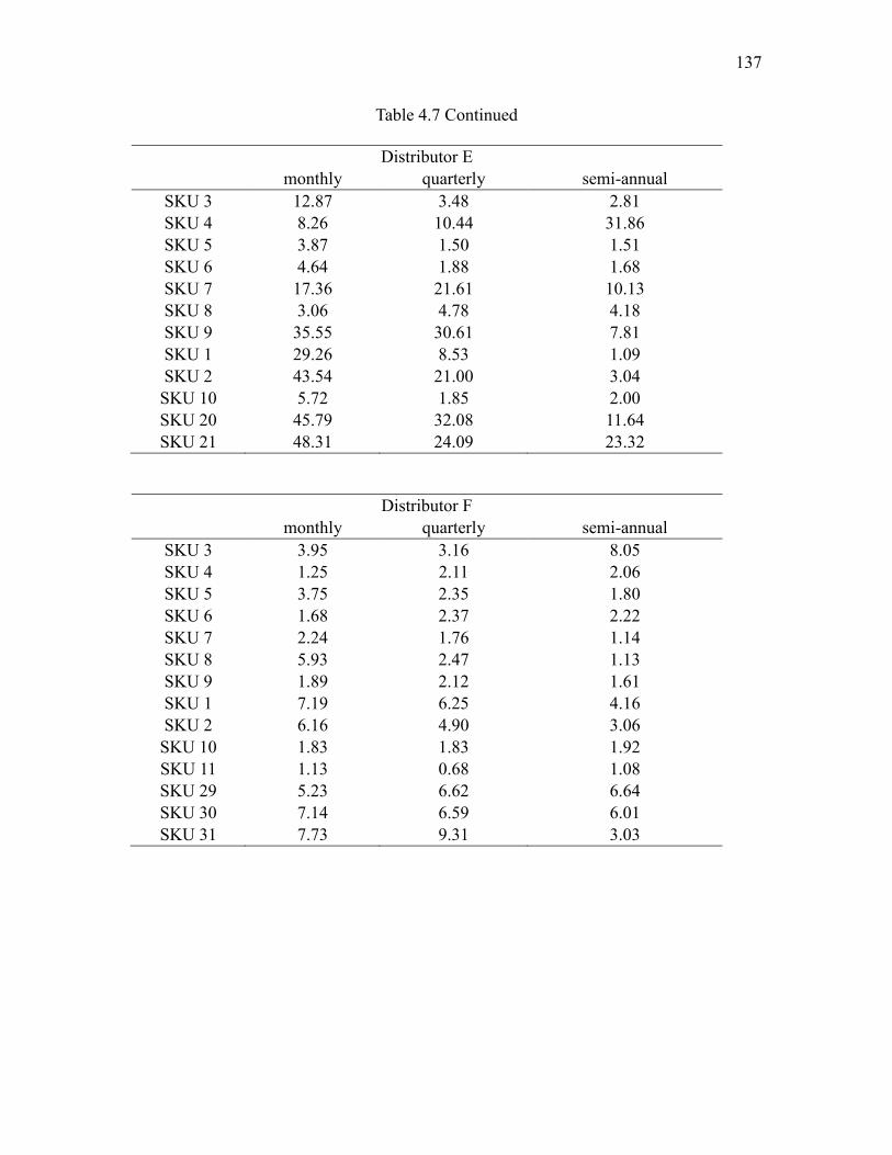
137
Table 4.7 Continued
Distributor E
monthly quarterly semi-annual
SKU 3 12.87 3.48 2.81
SKU 4 8.26 10.44 31.86
SKU 5 3.87 1.50 1.51
SKU 6 4.64 1.88 1.68
SKU 7 17.36 21.61 10.13
SKU 8 3.06 4.78 4.18
SKU 9 35.55 30.61 7.81
SKU 1 29.26 8.53 1.09
SKU 2 43.54 21.00 3.04
SKU 10 5.72 1.85 2.00
SKU 20 45.79 32.08 11.64
SKU 21 48.31 24.09 23.32
Distributor F
monthly quarterly semi-annual
SKU 3 3.95 3.16 8.05
SKU 4 1.25 2.11 2.06
SKU 5 3.75 2.35 1.80
SKU 6 1.68 2.37 2.22
SKU 7 2.24 1.76 1.14
SKU 8 5.93 2.47 1.13
SKU 9 1.89 2.12 1.61
SKU 1 7.19 6.25 4.16
SKU 2 6.16 4.90 3.06
SKU 10 1.83 1.83 1.92
SKU 11 1.13 0.68 1.08
SKU 29 5.23 6.62 6.64
SKU 30 7.14 6.59 6.01
SKU 31 7.73 9.31 3.03
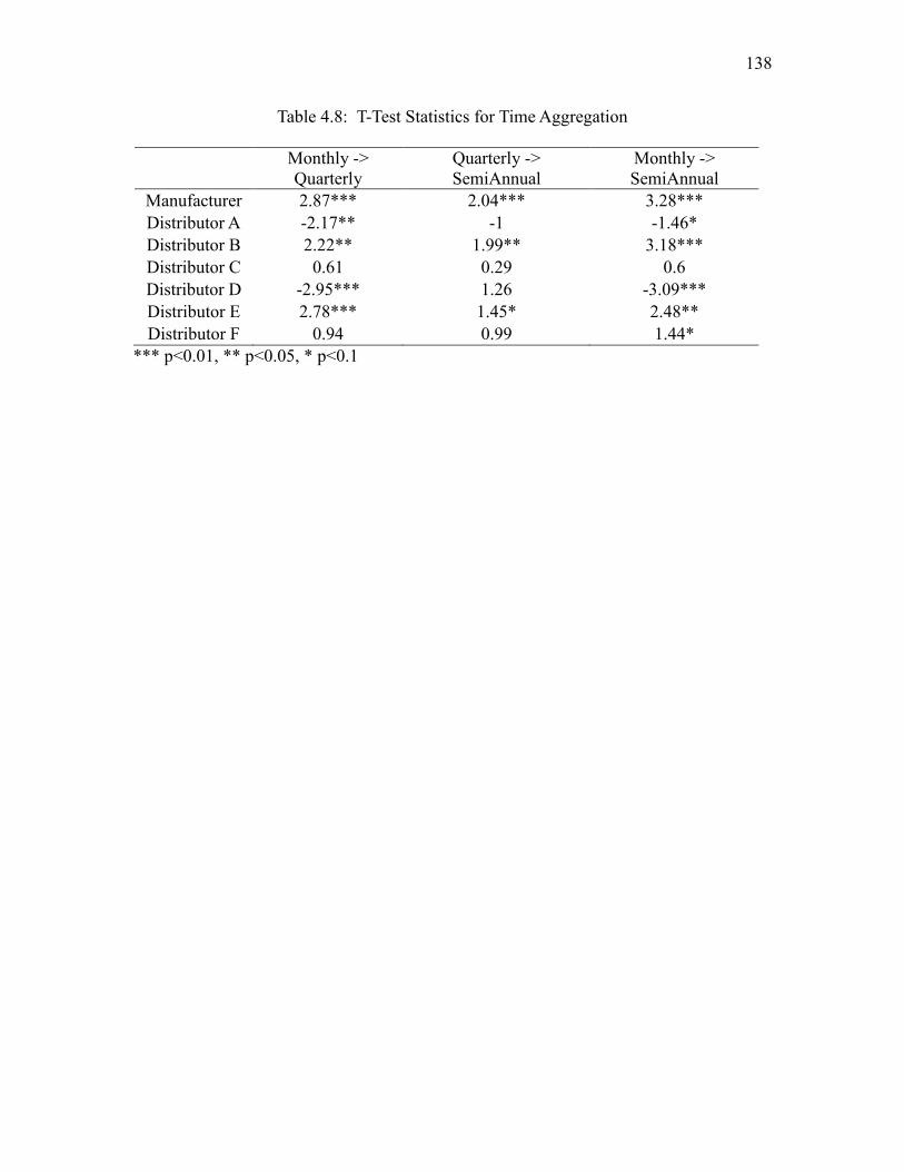
138
Table 4.8: T-Test Statistics for Time Aggregation
Monthly ->
Quarterly
Quarterly ->
SemiAnnual
Monthly ->
SemiAnnual
Manufacturer 2.87*** 2.04*** 3.28***
Distributor A -2.17** -1 -1.46*
Distributor B 2.22** 1.99** 3.18***
Distributor C 0.61 0.29 0.6
Distributor D -2.95*** 1.26 -3.09***
Distributor E 2.78*** 1.45* 2.48**
Distributor F 0.94 0.99 1.44*
*** p<0.01, ** p<0.05, * p<0.1
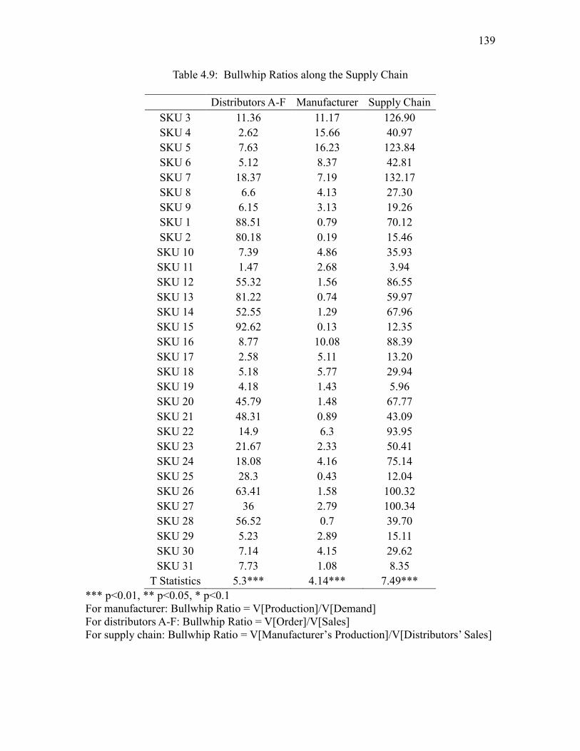
139
Table 4.9: Bullwhip Ratios along the Supply Chain
Distributors A-F Manufacturer Supply Chain
SKU 3 11.36 11.17 126.90
SKU 4 2.62 15.66 40.97
SKU 5 7.63 16.23 123.84
SKU 6 5.12 8.37 42.81
SKU 7 18.37 7.19 132.17
SKU 8 6.6 4.13 27.30
SKU 9 6.15 3.13 19.26
SKU 1 88.51 0.79 70.12
SKU 2 80.18 0.19 15.46
SKU 10 7.39 4.86 35.93
SKU 11 1.47 2.68 3.94
SKU 12 55.32 1.56 86.55
SKU 13 81.22 0.74 59.97
SKU 14 52.55 1.29 67.96
SKU 15 92.62 0.13 12.35
SKU 16 8.77 10.08 88.39
SKU 17 2.58 5.11 13.20
SKU 18 5.18 5.77 29.94
SKU 19 4.18 1.43 5.96
SKU 20 45.79 1.48 67.77
SKU 21 48.31 0.89 43.09
SKU 22 14.9 6.3 93.95
SKU 23 21.67 2.33 50.41
SKU 24 18.08 4.16 75.14
SKU 25 28.3 0.43 12.04
SKU 26 63.41 1.58 100.32
SKU 27 36 2.79 100.34
SKU 28 56.52 0.7 39.70
SKU 29 5.23 2.89 15.11
SKU 30 7.14 4.15 29.62
SKU 31 7.73 1.08 8.35
T Statistics 5.3*** 4.14*** 7.49***
*** p<0.01, ** p<0.05, * p<0.1
For manufacturer: Bullwhip Ratio = V[Production]/V[Demand]
For distributors A-F: Bullwhip Ratio = V[Order]/V[Sales]
For supply chain: Bullwhip Ratio = V[Manufacturer’s Production]/V[Distributors’ Sales]
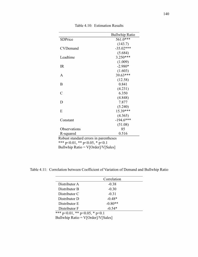
140
Table 4.10: Estimation Results
Bullwhip Ratio
SDPrice 561.0***
(143.7)
CVDemand -35.02***
(5.684)
Leadtime 3.250***
(1.009)
IR -2.980*
(1.603)
A 39.63***
(12.58)
B 0.841
(4.231)
C 6.350
(4.848)
D 7.877
(5.240)
E 15.39***
(4.365)
Constant -194.6***
(51.08)
Observations 85
R-squared 0.516
Robust standard errors in parentheses
*** p<0.01, ** p<0.05, * p<0.1
Bullwhip Ratio = V[Order]/V[Sales]
Table 4.11: Correlation between Coefficient of Variation of Demand and Bullwhip Ratio
Correlation
Distributor A -0.38
Distributor B -0.30
Distributor C -0.31
Distributor D -0.48*
Distributor E -0.80**
Distributor F -0.54*
*** p<0.01, ** p<0.05, * p<0.1
Bullwhip Ratio = V[Order]/V[Sales]
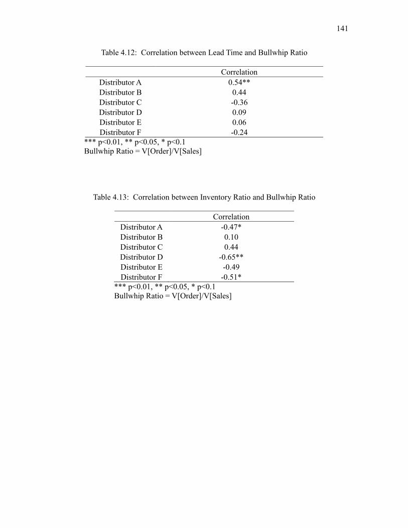
141
Table 4.12: Correlation between Lead Time and Bullwhip Ratio
Correlation
Distributor A 0.54**
Distributor B 0.44
Distributor C -0.36
Distributor D 0.09
Distributor E 0.06
Distributor F -0.24
*** p<0.01, ** p<0.05, * p<0.1
Bullwhip Ratio = V[Order]/V[Sales]
Table 4.13: Correlation between Inventory Ratio and Bullwhip Ratio
Correlation
Distributor A -0.47*
Distributor B 0.10
Distributor C 0.44
Distributor D -0.65**
Distributor E -0.49
Distributor F -0.51*
*** p<0.01, ** p<0.05, * p<0.1
Bullwhip Ratio = V[Order]/V[Sales]
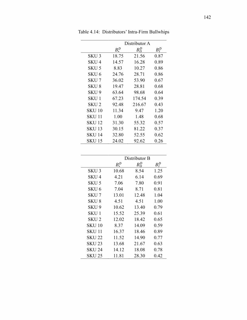
142
Table 4.14: Distributors’ Intra-Firm Bullwhips
Distributor A
𝐵∗𝐷 𝐵𝑂
𝐷 𝐵𝐼𝐷
SKU 3 18.75 21.56 0.87
SKU 4 14.57 16.28 0.89
SKU 5 8.83 10.27 0.86
SKU 6 24.76 28.71 0.86
SKU 7 36.02 53.90 0.67
SKU 8 19.47 28.81 0.68
SKU 9 63.64 98.68 0.64
SKU 1 67.23 174.54 0.39
SKU 2 92.48 216.67 0.43
SKU 10 11.34 9.47 1.20
SKU 11 1.00 1.48 0.68
SKU 12 31.30 55.32 0.57
SKU 13 30.15 81.22 0.37
SKU 14 32.80 52.55 0.62
SKU 15 24.02 92.62 0.26
Distributor B
𝐵∗𝐷 𝐵𝑂
𝐷 𝐵𝐼𝐷
SKU 3 10.68 8.54 1.25
SKU 4 4.21 6.14 0.69
SKU 5 7.06 7.80 0.91
SKU 6 7.04 8.71 0.81
SKU 7 13.01 12.48 1.04
SKU 8 4.51 4.51 1.00
SKU 9 10.62 13.40 0.79
SKU 1 15.52 25.39 0.61
SKU 2 12.02 18.42 0.65
SKU 10 8.37 14.09 0.59
SKU 11 16.37 18.46 0.89
SKU 22 11.52 14.90 0.77
SKU 23 13.68 21.67 0.63
SKU 24 14.12 18.08 0.78
SKU 25 11.81 28.30 0.42
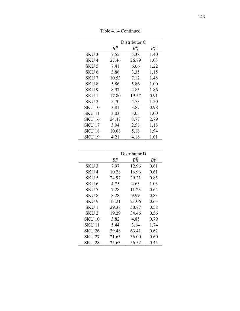
143
Table 4.14 Continued
Distributor C
𝐵∗𝐷 𝐵𝑂
𝐷 𝐵𝐼𝐷
SKU 3 7.55 5.38 1.40
SKU 4 27.46 26.79 1.03
SKU 5 7.41 6.06 1.22
SKU 6 3.86 3.35 1.15
SKU 7 10.53 7.12 1.48
SKU 8 5.86 5.86 1.00
SKU 9 8.97 4.83 1.86
SKU 1 17.80 19.57 0.91
SKU 2 5.70 4.73 1.20
SKU 10 3.81 3.87 0.98
SKU 11 3.03 3.03 1.00
SKU 16 24.47 8.77 2.79
SKU 17 3.04 2.58 1.18
SKU 18 10.08 5.18 1.94
SKU 19 4.21 4.18 1.01
Distributor D
𝐵∗𝐷 𝐵𝑂
𝐷 𝐵𝐼𝐷
SKU 3 7.97 12.96 0.61
SKU 4 10.28 16.96 0.61
SKU 5 24.97 29.21 0.85
SKU 6 4.75 4.63 1.03
SKU 7 7.28 11.23 0.65
SKU 8 8.28 9.99 0.83
SKU 9 13.21 21.06 0.63
SKU 1 29.38 50.77 0.58
SKU 2 19.29 34.46 0.56
SKU 10 3.82 4.85 0.79
SKU 11 5.44 3.14 1.74
SKU 26 39.48 63.41 0.62
SKU 27 21.65 36.00 0.60
SKU 28 25.63 56.52 0.45
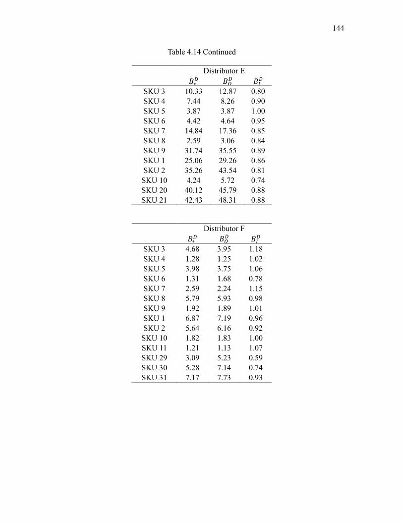
144
Table 4.14 Continued
Distributor E
𝐵∗𝐷 𝐵𝑂
𝐷 𝐵𝐼𝐷
SKU 3 10.33 12.87 0.80
SKU 4 7.44 8.26 0.90
SKU 5 3.87 3.87 1.00
SKU 6 4.42 4.64 0.95
SKU 7 14.84 17.36 0.85
SKU 8 2.59 3.06 0.84
SKU 9 31.74 35.55 0.89
SKU 1 25.06 29.26 0.86
SKU 2 35.26 43.54 0.81
SKU 10 4.24 5.72 0.74
SKU 20 40.12 45.79 0.88
SKU 21 42.43 48.31 0.88
Distributor F
𝐵∗𝐷 𝐵𝑂
𝐷 𝐵𝐼𝐷
SKU 3 4.68 3.95 1.18
SKU 4 1.28 1.25 1.02
SKU 5 3.98 3.75 1.06
SKU 6 1.31 1.68 0.78
SKU 7 2.59 2.24 1.15
SKU 8 5.79 5.93 0.98
SKU 9 1.92 1.89 1.01
SKU 1 6.87 7.19 0.96
SKU 2 5.64 6.16 0.92
SKU 10 1.82 1.83 1.00
SKU 11 1.21 1.13 1.07
SKU 29 3.09 5.23 0.59
SKU 30 5.28 7.14 0.74
SKU 31 7.17 7.73 0.93
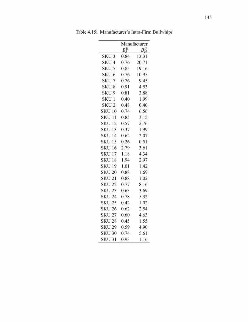
145
Table 4.15: Manufacturer’s Intra-Firm Bullwhips
Manufacturer
𝐵𝑆𝑈 𝐵𝑀
𝑈
SKU 3 0.84 13.31
SKU 4 0.76 20.71
SKU 5 0.85 19.16
SKU 6 0.76 10.95
SKU 7 0.76 9.45
SKU 8 0.91 4.53
SKU 9 0.81 3.88
SKU 1 0.40 1.99
SKU 2 0.48 0.40
SKU 10 0.74 6.56
SKU 11 0.85 3.15
SKU 12 0.57 2.76
SKU 13 0.37 1.99
SKU 14 0.62 2.07
SKU 15 0.26 0.51
SKU 16 2.79 3.61
SKU 17 1.18 4.34
SKU 18 1.94 2.97
SKU 19 1.01 1.42
SKU 20 0.88 1.69
SKU 21 0.88 1.02
SKU 22 0.77 8.16
SKU 23 0.63 3.69
SKU 24 0.78 5.32
SKU 25 0.42 1.02
SKU 26 0.62 2.54
SKU 27 0.60 4.63
SKU 28 0.45 1.55
SKU 29 0.59 4.90
SKU 30 0.74 5.61
SKU 31 0.93 1.16
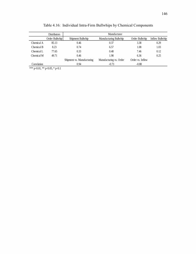
146
Table 4.16: Individual Intra-Firm Bullwhips by Chemical Components
Distributors
Order Bullwhip Shipment Bullwhip Manufacturing Bullwhip Order Bullwhip Inflow Bullwhip
Chemical A 85.13 0.46 0.37 3.38 0.29
Chemical B 8.23 0.74 6.57 1.08 1.03
Chemical L 77.65 0.33 0.48 7.46 0.12
Chemical M 49.71 0.46 1.98 6.36 0.25
Shipment vs. Manufacturing Manufacturing vs. Order Order vs. Inflow
Correlation 0.94 -0.73 -0.88
*** p<0.01, ** p<0.05, * p<0.1
Manufacturer
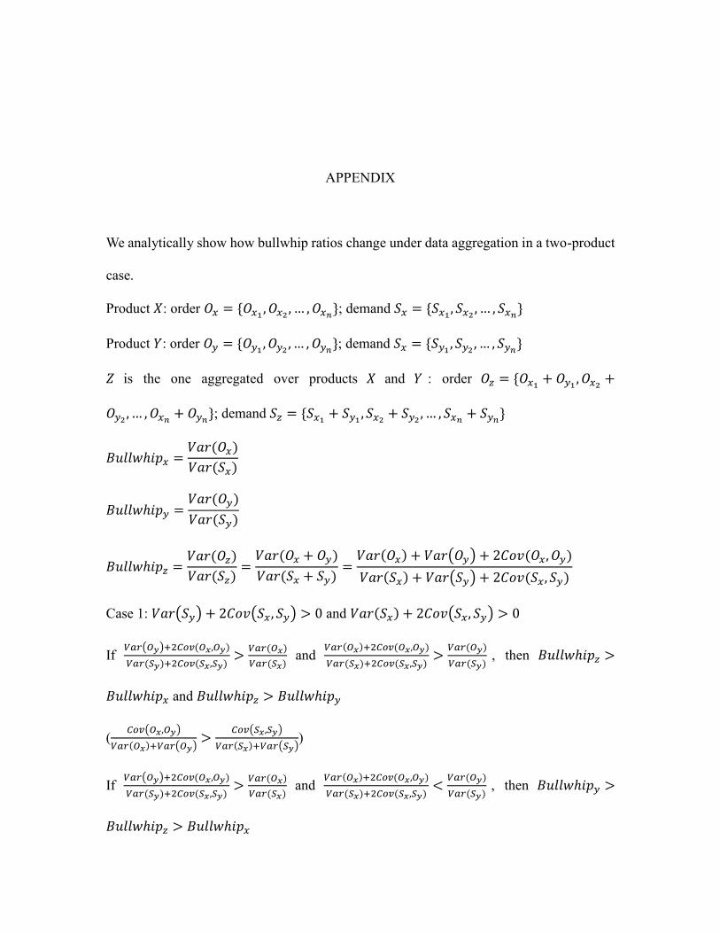
APPENDIX
We analytically show how bullwhip ratios change under data aggregation in a two-product
case.
Product 𝑋: order 𝑂𝑥 = {𝑂𝑥1, 𝑂𝑥2
, … , 𝑂𝑥𝑛}; demand 𝑆𝑥 = {𝑆𝑥1
, 𝑆𝑥2, … , 𝑆𝑥𝑛
}
Product 𝑌: order 𝑂𝑦 = {𝑂𝑦1, 𝑂𝑦2
, … , 𝑂𝑦𝑛}; demand 𝑆𝑥 = {𝑆𝑦1
, 𝑆𝑦2, … , 𝑆𝑦𝑛
}
𝑍 is the one aggregated over products 𝑋 and 𝑌 : order 𝑂𝑧 = {𝑂𝑥1+ 𝑂𝑦1
, 𝑂𝑥2+
𝑂𝑦2, … , 𝑂𝑥𝑛
+ 𝑂𝑦𝑛}; demand 𝑆𝑧 = {𝑆𝑥1
+ 𝑆𝑦1, 𝑆𝑥2
+ 𝑆𝑦2, … , 𝑆𝑥𝑛
+ 𝑆𝑦𝑛}
𝐵𝑢𝑙𝑙𝑤ℎ𝑖𝑝𝑥 =𝑉𝑎𝑟(𝑂𝑥)
𝑉𝑎𝑟(𝑆𝑥)
𝐵𝑢𝑙𝑙𝑤ℎ𝑖𝑝𝑦 =𝑉𝑎𝑟(𝑂𝑦)
𝑉𝑎𝑟(𝑆𝑦)
𝐵𝑢𝑙𝑙𝑤ℎ𝑖𝑝𝑧 =𝑉𝑎𝑟(𝑂𝑧)
𝑉𝑎𝑟(𝑆𝑧)=
𝑉𝑎𝑟(𝑂𝑥 + 𝑂𝑦)
𝑉𝑎𝑟(𝑆𝑥 + 𝑆𝑦)=
𝑉𝑎𝑟(𝑂𝑥) + 𝑉𝑎𝑟(𝑂𝑦) + 2𝐶𝑜𝑣(𝑂𝑥, 𝑂𝑦)
𝑉𝑎𝑟(𝑆𝑥) + 𝑉𝑎𝑟(𝑆𝑦) + 2𝐶𝑜𝑣(𝑆𝑥, 𝑆𝑦)
Case 1: 𝑉𝑎𝑟(𝑆𝑦) + 2𝐶𝑜𝑣(𝑆𝑥, 𝑆𝑦) > 0 and 𝑉𝑎𝑟(𝑆𝑥) + 2𝐶𝑜𝑣(𝑆𝑥, 𝑆𝑦) > 0
If 𝑉𝑎𝑟(𝑂𝑦)+2𝐶𝑜𝑣(𝑂𝑥,𝑂𝑦)
𝑉𝑎𝑟(𝑆𝑦)+2𝐶𝑜𝑣(𝑆𝑥,𝑆𝑦)>
𝑉𝑎𝑟(𝑂𝑥)
𝑉𝑎𝑟(𝑆𝑥) and
𝑉𝑎𝑟(𝑂𝑥)+2𝐶𝑜𝑣(𝑂𝑥,𝑂𝑦)
𝑉𝑎𝑟(𝑆𝑥)+2𝐶𝑜𝑣(𝑆𝑥,𝑆𝑦)>
𝑉𝑎𝑟(𝑂𝑦)
𝑉𝑎𝑟(𝑆𝑦) , then 𝐵𝑢𝑙𝑙𝑤ℎ𝑖𝑝𝑧 >
𝐵𝑢𝑙𝑙𝑤ℎ𝑖𝑝𝑥 and 𝐵𝑢𝑙𝑙𝑤ℎ𝑖𝑝𝑧 > 𝐵𝑢𝑙𝑙𝑤ℎ𝑖𝑝𝑦
(𝐶𝑜𝑣(𝑂𝑥,𝑂𝑦)
𝑉𝑎𝑟(𝑂𝑥)+𝑉𝑎𝑟(𝑂𝑦)>
𝐶𝑜𝑣(𝑆𝑥,𝑆𝑦)
𝑉𝑎𝑟(𝑆𝑥)+𝑉𝑎𝑟(𝑆𝑦))
If 𝑉𝑎𝑟(𝑂𝑦)+2𝐶𝑜𝑣(𝑂𝑥,𝑂𝑦)
𝑉𝑎𝑟(𝑆𝑦)+2𝐶𝑜𝑣(𝑆𝑥,𝑆𝑦)>
𝑉𝑎𝑟(𝑂𝑥)
𝑉𝑎𝑟(𝑆𝑥) and
𝑉𝑎𝑟(𝑂𝑥)+2𝐶𝑜𝑣(𝑂𝑥,𝑂𝑦)
𝑉𝑎𝑟(𝑆𝑥)+2𝐶𝑜𝑣(𝑆𝑥,𝑆𝑦)<
𝑉𝑎𝑟(𝑂𝑦)
𝑉𝑎𝑟(𝑆𝑦) , then 𝐵𝑢𝑙𝑙𝑤ℎ𝑖𝑝𝑦 >
𝐵𝑢𝑙𝑙𝑤ℎ𝑖𝑝𝑧 > 𝐵𝑢𝑙𝑙𝑤ℎ𝑖𝑝𝑥
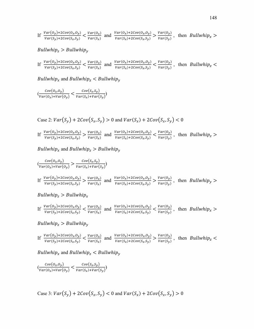
148
If 𝑉𝑎𝑟(𝑂𝑦)+2𝐶𝑜𝑣(𝑂𝑥,𝑂𝑦)
𝑉𝑎𝑟(𝑆𝑦)+2𝐶𝑜𝑣(𝑆𝑥,𝑆𝑦)<
𝑉𝑎𝑟(𝑂𝑥)
𝑉𝑎𝑟(𝑆𝑥) and
𝑉𝑎𝑟(𝑂𝑥)+2𝐶𝑜𝑣(𝑂𝑥,𝑂𝑦)
𝑉𝑎𝑟(𝑆𝑥)+2𝐶𝑜𝑣(𝑆𝑥,𝑆𝑦)>
𝑉𝑎𝑟(𝑂𝑦)
𝑉𝑎𝑟(𝑆𝑦) , then 𝐵𝑢𝑙𝑙𝑤ℎ𝑖𝑝𝑥 >
𝐵𝑢𝑙𝑙𝑤ℎ𝑖𝑝𝑧 > 𝐵𝑢𝑙𝑙𝑤ℎ𝑖𝑝𝑦
If 𝑉𝑎𝑟(𝑂𝑦)+2𝐶𝑜𝑣(𝑂𝑥,𝑂𝑦)
𝑉𝑎𝑟(𝑆𝑦)+2𝐶𝑜𝑣(𝑆𝑥,𝑆𝑦)<
𝑉𝑎𝑟(𝑂𝑥)
𝑉𝑎𝑟(𝑆𝑥) and
𝑉𝑎𝑟(𝑂𝑥)+2𝐶𝑜𝑣(𝑂𝑥,𝑂𝑦)
𝑉𝑎𝑟(𝑆𝑥)+2𝐶𝑜𝑣(𝑆𝑥,𝑆𝑦)<
𝑉𝑎𝑟(𝑂𝑦)
𝑉𝑎𝑟(𝑆𝑦) , then 𝐵𝑢𝑙𝑙𝑤ℎ𝑖𝑝𝑧 <
𝐵𝑢𝑙𝑙𝑤ℎ𝑖𝑝𝑥 and 𝐵𝑢𝑙𝑙𝑤ℎ𝑖𝑝𝑧 < 𝐵𝑢𝑙𝑙𝑤ℎ𝑖𝑝𝑦
(𝐶𝑜𝑣(𝑂𝑥,𝑂𝑦)
𝑉𝑎𝑟(𝑂𝑥)+𝑉𝑎𝑟(𝑂𝑦)<
𝐶𝑜𝑣(𝑆𝑥,𝑆𝑦)
𝑉𝑎𝑟(𝑆𝑥)+𝑉𝑎𝑟(𝑆𝑦))
Case 2: 𝑉𝑎𝑟(𝑆𝑦) + 2𝐶𝑜𝑣(𝑆𝑥, 𝑆𝑦) > 0 and 𝑉𝑎𝑟(𝑆𝑥) + 2𝐶𝑜𝑣(𝑆𝑥, 𝑆𝑦) < 0
If 𝑉𝑎𝑟(𝑂𝑦)+2𝐶𝑜𝑣(𝑂𝑥,𝑂𝑦)
𝑉𝑎𝑟(𝑆𝑦)+2𝐶𝑜𝑣(𝑆𝑥,𝑆𝑦)>
𝑉𝑎𝑟(𝑂𝑥)
𝑉𝑎𝑟(𝑆𝑥) and
𝑉𝑎𝑟(𝑂𝑥)+2𝐶𝑜𝑣(𝑂𝑥,𝑂𝑦)
𝑉𝑎𝑟(𝑆𝑥)+2𝐶𝑜𝑣(𝑆𝑥,𝑆𝑦)<
𝑉𝑎𝑟(𝑂𝑦)
𝑉𝑎𝑟(𝑆𝑦) , then 𝐵𝑢𝑙𝑙𝑤ℎ𝑖𝑝𝑧 >
𝐵𝑢𝑙𝑙𝑤ℎ𝑖𝑝𝑥 and 𝐵𝑢𝑙𝑙𝑤ℎ𝑖𝑝𝑧 > 𝐵𝑢𝑙𝑙𝑤ℎ𝑖𝑝𝑦
(𝐶𝑜𝑣(𝑂𝑥,𝑂𝑦)
𝑉𝑎𝑟(𝑂𝑥)+𝑉𝑎𝑟(𝑂𝑦)>
𝐶𝑜𝑣(𝑆𝑥,𝑆𝑦)
𝑉𝑎𝑟(𝑆𝑥)+𝑉𝑎𝑟(𝑆𝑦))
If 𝑉𝑎𝑟(𝑂𝑦)+2𝐶𝑜𝑣(𝑂𝑥,𝑂𝑦)
𝑉𝑎𝑟(𝑆𝑦)+2𝐶𝑜𝑣(𝑆𝑥,𝑆𝑦)>
𝑉𝑎𝑟(𝑂𝑥)
𝑉𝑎𝑟(𝑆𝑥) and
𝑉𝑎𝑟(𝑂𝑥)+2𝐶𝑜𝑣(𝑂𝑥,𝑂𝑦)
𝑉𝑎𝑟(𝑆𝑥)+2𝐶𝑜𝑣(𝑆𝑥,𝑆𝑦)>
𝑉𝑎𝑟(𝑂𝑦)
𝑉𝑎𝑟(𝑆𝑦) , then 𝐵𝑢𝑙𝑙𝑤ℎ𝑖𝑝𝑦 >
𝐵𝑢𝑙𝑙𝑤ℎ𝑖𝑝𝑧 > 𝐵𝑢𝑙𝑙𝑤ℎ𝑖𝑝𝑥
If 𝑉𝑎𝑟(𝑂𝑦)+2𝐶𝑜𝑣(𝑂𝑥,𝑂𝑦)
𝑉𝑎𝑟(𝑆𝑦)+2𝐶𝑜𝑣(𝑆𝑥,𝑆𝑦)<
𝑉𝑎𝑟(𝑂𝑥)
𝑉𝑎𝑟(𝑆𝑥) and
𝑉𝑎𝑟(𝑂𝑥)+2𝐶𝑜𝑣(𝑂𝑥,𝑂𝑦)
𝑉𝑎𝑟(𝑆𝑥)+2𝐶𝑜𝑣(𝑆𝑥,𝑆𝑦)<
𝑉𝑎𝑟(𝑂𝑦)
𝑉𝑎𝑟(𝑆𝑦) , then 𝐵𝑢𝑙𝑙𝑤ℎ𝑖𝑝𝑥 >
𝐵𝑢𝑙𝑙𝑤ℎ𝑖𝑝𝑧 > 𝐵𝑢𝑙𝑙𝑤ℎ𝑖𝑝𝑦
If 𝑉𝑎𝑟(𝑂𝑦)+2𝐶𝑜𝑣(𝑂𝑥,𝑂𝑦)
𝑉𝑎𝑟(𝑆𝑦)+2𝐶𝑜𝑣(𝑆𝑥,𝑆𝑦)<
𝑉𝑎𝑟(𝑂𝑥)
𝑉𝑎𝑟(𝑆𝑥) and
𝑉𝑎𝑟(𝑂𝑥)+2𝐶𝑜𝑣(𝑂𝑥,𝑂𝑦)
𝑉𝑎𝑟(𝑆𝑥)+2𝐶𝑜𝑣(𝑆𝑥,𝑆𝑦)>
𝑉𝑎𝑟(𝑂𝑦)
𝑉𝑎𝑟(𝑆𝑦) , then 𝐵𝑢𝑙𝑙𝑤ℎ𝑖𝑝𝑧 <
𝐵𝑢𝑙𝑙𝑤ℎ𝑖𝑝𝑥 and 𝐵𝑢𝑙𝑙𝑤ℎ𝑖𝑝𝑧 < 𝐵𝑢𝑙𝑙𝑤ℎ𝑖𝑝𝑦
(𝐶𝑜𝑣(𝑂𝑥,𝑂𝑦)
𝑉𝑎𝑟(𝑂𝑥)+𝑉𝑎𝑟(𝑂𝑦)<
𝐶𝑜𝑣(𝑆𝑥,𝑆𝑦)
𝑉𝑎𝑟(𝑆𝑥)+𝑉𝑎𝑟(𝑆𝑦))
Case 3: 𝑉𝑎𝑟(𝑆𝑦) + 2𝐶𝑜𝑣(𝑆𝑥, 𝑆𝑦) < 0 and 𝑉𝑎𝑟(𝑆𝑥) + 2𝐶𝑜𝑣(𝑆𝑥, 𝑆𝑦) > 0
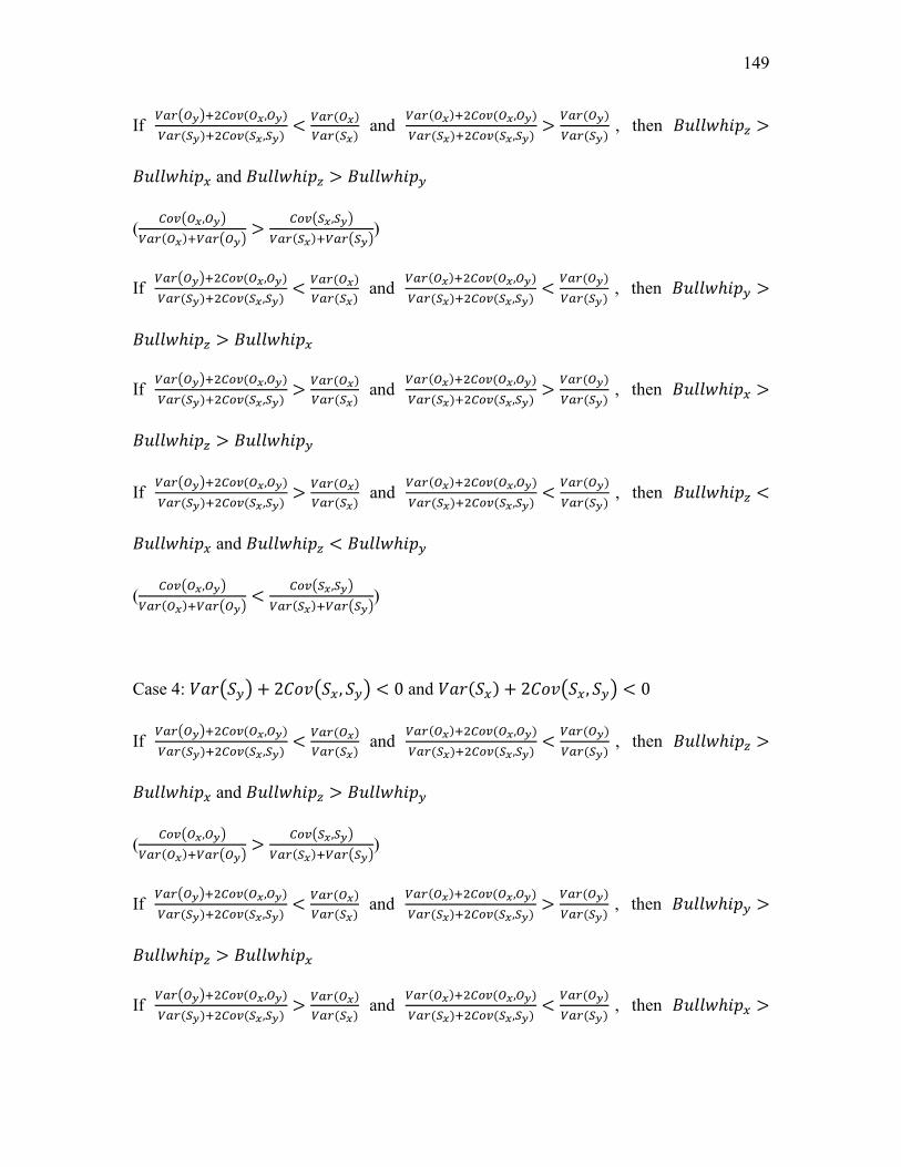
149
If 𝑉𝑎𝑟(𝑂𝑦)+2𝐶𝑜𝑣(𝑂𝑥,𝑂𝑦)
𝑉𝑎𝑟(𝑆𝑦)+2𝐶𝑜𝑣(𝑆𝑥,𝑆𝑦)<
𝑉𝑎𝑟(𝑂𝑥)
𝑉𝑎𝑟(𝑆𝑥) and
𝑉𝑎𝑟(𝑂𝑥)+2𝐶𝑜𝑣(𝑂𝑥,𝑂𝑦)
𝑉𝑎𝑟(𝑆𝑥)+2𝐶𝑜𝑣(𝑆𝑥,𝑆𝑦)>
𝑉𝑎𝑟(𝑂𝑦)
𝑉𝑎𝑟(𝑆𝑦) , then 𝐵𝑢𝑙𝑙𝑤ℎ𝑖𝑝𝑧 >
𝐵𝑢𝑙𝑙𝑤ℎ𝑖𝑝𝑥 and 𝐵𝑢𝑙𝑙𝑤ℎ𝑖𝑝𝑧 > 𝐵𝑢𝑙𝑙𝑤ℎ𝑖𝑝𝑦
(𝐶𝑜𝑣(𝑂𝑥,𝑂𝑦)
𝑉𝑎𝑟(𝑂𝑥)+𝑉𝑎𝑟(𝑂𝑦)>
𝐶𝑜𝑣(𝑆𝑥,𝑆𝑦)
𝑉𝑎𝑟(𝑆𝑥)+𝑉𝑎𝑟(𝑆𝑦))
If 𝑉𝑎𝑟(𝑂𝑦)+2𝐶𝑜𝑣(𝑂𝑥,𝑂𝑦)
𝑉𝑎𝑟(𝑆𝑦)+2𝐶𝑜𝑣(𝑆𝑥,𝑆𝑦)<
𝑉𝑎𝑟(𝑂𝑥)
𝑉𝑎𝑟(𝑆𝑥) and
𝑉𝑎𝑟(𝑂𝑥)+2𝐶𝑜𝑣(𝑂𝑥,𝑂𝑦)
𝑉𝑎𝑟(𝑆𝑥)+2𝐶𝑜𝑣(𝑆𝑥,𝑆𝑦)<
𝑉𝑎𝑟(𝑂𝑦)
𝑉𝑎𝑟(𝑆𝑦) , then 𝐵𝑢𝑙𝑙𝑤ℎ𝑖𝑝𝑦 >
𝐵𝑢𝑙𝑙𝑤ℎ𝑖𝑝𝑧 > 𝐵𝑢𝑙𝑙𝑤ℎ𝑖𝑝𝑥
If 𝑉𝑎𝑟(𝑂𝑦)+2𝐶𝑜𝑣(𝑂𝑥,𝑂𝑦)
𝑉𝑎𝑟(𝑆𝑦)+2𝐶𝑜𝑣(𝑆𝑥,𝑆𝑦)>
𝑉𝑎𝑟(𝑂𝑥)
𝑉𝑎𝑟(𝑆𝑥) and
𝑉𝑎𝑟(𝑂𝑥)+2𝐶𝑜𝑣(𝑂𝑥,𝑂𝑦)
𝑉𝑎𝑟(𝑆𝑥)+2𝐶𝑜𝑣(𝑆𝑥,𝑆𝑦)>
𝑉𝑎𝑟(𝑂𝑦)
𝑉𝑎𝑟(𝑆𝑦) , then 𝐵𝑢𝑙𝑙𝑤ℎ𝑖𝑝𝑥 >
𝐵𝑢𝑙𝑙𝑤ℎ𝑖𝑝𝑧 > 𝐵𝑢𝑙𝑙𝑤ℎ𝑖𝑝𝑦
If 𝑉𝑎𝑟(𝑂𝑦)+2𝐶𝑜𝑣(𝑂𝑥,𝑂𝑦)
𝑉𝑎𝑟(𝑆𝑦)+2𝐶𝑜𝑣(𝑆𝑥,𝑆𝑦)>
𝑉𝑎𝑟(𝑂𝑥)
𝑉𝑎𝑟(𝑆𝑥) and
𝑉𝑎𝑟(𝑂𝑥)+2𝐶𝑜𝑣(𝑂𝑥,𝑂𝑦)
𝑉𝑎𝑟(𝑆𝑥)+2𝐶𝑜𝑣(𝑆𝑥,𝑆𝑦)<
𝑉𝑎𝑟(𝑂𝑦)
𝑉𝑎𝑟(𝑆𝑦) , then 𝐵𝑢𝑙𝑙𝑤ℎ𝑖𝑝𝑧 <
𝐵𝑢𝑙𝑙𝑤ℎ𝑖𝑝𝑥 and 𝐵𝑢𝑙𝑙𝑤ℎ𝑖𝑝𝑧 < 𝐵𝑢𝑙𝑙𝑤ℎ𝑖𝑝𝑦
(𝐶𝑜𝑣(𝑂𝑥,𝑂𝑦)
𝑉𝑎𝑟(𝑂𝑥)+𝑉𝑎𝑟(𝑂𝑦)<
𝐶𝑜𝑣(𝑆𝑥,𝑆𝑦)
𝑉𝑎𝑟(𝑆𝑥)+𝑉𝑎𝑟(𝑆𝑦))
Case 4: 𝑉𝑎𝑟(𝑆𝑦) + 2𝐶𝑜𝑣(𝑆𝑥, 𝑆𝑦) < 0 and 𝑉𝑎𝑟(𝑆𝑥) + 2𝐶𝑜𝑣(𝑆𝑥, 𝑆𝑦) < 0
If 𝑉𝑎𝑟(𝑂𝑦)+2𝐶𝑜𝑣(𝑂𝑥,𝑂𝑦)
𝑉𝑎𝑟(𝑆𝑦)+2𝐶𝑜𝑣(𝑆𝑥,𝑆𝑦)<
𝑉𝑎𝑟(𝑂𝑥)
𝑉𝑎𝑟(𝑆𝑥) and
𝑉𝑎𝑟(𝑂𝑥)+2𝐶𝑜𝑣(𝑂𝑥,𝑂𝑦)
𝑉𝑎𝑟(𝑆𝑥)+2𝐶𝑜𝑣(𝑆𝑥,𝑆𝑦)<
𝑉𝑎𝑟(𝑂𝑦)
𝑉𝑎𝑟(𝑆𝑦) , then 𝐵𝑢𝑙𝑙𝑤ℎ𝑖𝑝𝑧 >
𝐵𝑢𝑙𝑙𝑤ℎ𝑖𝑝𝑥 and 𝐵𝑢𝑙𝑙𝑤ℎ𝑖𝑝𝑧 > 𝐵𝑢𝑙𝑙𝑤ℎ𝑖𝑝𝑦
(𝐶𝑜𝑣(𝑂𝑥,𝑂𝑦)
𝑉𝑎𝑟(𝑂𝑥)+𝑉𝑎𝑟(𝑂𝑦)>
𝐶𝑜𝑣(𝑆𝑥,𝑆𝑦)
𝑉𝑎𝑟(𝑆𝑥)+𝑉𝑎𝑟(𝑆𝑦))
If 𝑉𝑎𝑟(𝑂𝑦)+2𝐶𝑜𝑣(𝑂𝑥,𝑂𝑦)
𝑉𝑎𝑟(𝑆𝑦)+2𝐶𝑜𝑣(𝑆𝑥,𝑆𝑦)<
𝑉𝑎𝑟(𝑂𝑥)
𝑉𝑎𝑟(𝑆𝑥) and
𝑉𝑎𝑟(𝑂𝑥)+2𝐶𝑜𝑣(𝑂𝑥,𝑂𝑦)
𝑉𝑎𝑟(𝑆𝑥)+2𝐶𝑜𝑣(𝑆𝑥,𝑆𝑦)>
𝑉𝑎𝑟(𝑂𝑦)
𝑉𝑎𝑟(𝑆𝑦) , then 𝐵𝑢𝑙𝑙𝑤ℎ𝑖𝑝𝑦 >
𝐵𝑢𝑙𝑙𝑤ℎ𝑖𝑝𝑧 > 𝐵𝑢𝑙𝑙𝑤ℎ𝑖𝑝𝑥
If 𝑉𝑎𝑟(𝑂𝑦)+2𝐶𝑜𝑣(𝑂𝑥,𝑂𝑦)
𝑉𝑎𝑟(𝑆𝑦)+2𝐶𝑜𝑣(𝑆𝑥,𝑆𝑦)>
𝑉𝑎𝑟(𝑂𝑥)
𝑉𝑎𝑟(𝑆𝑥) and
𝑉𝑎𝑟(𝑂𝑥)+2𝐶𝑜𝑣(𝑂𝑥,𝑂𝑦)
𝑉𝑎𝑟(𝑆𝑥)+2𝐶𝑜𝑣(𝑆𝑥,𝑆𝑦)<
𝑉𝑎𝑟(𝑂𝑦)
𝑉𝑎𝑟(𝑆𝑦) , then 𝐵𝑢𝑙𝑙𝑤ℎ𝑖𝑝𝑥 >
150
𝐵𝑢𝑙𝑙𝑤ℎ𝑖𝑝𝑧 > 𝐵𝑢𝑙𝑙𝑤ℎ𝑖𝑝𝑦
If 𝑉𝑎𝑟(𝑂𝑦)+2𝐶𝑜𝑣(𝑂𝑥,𝑂𝑦)
𝑉𝑎𝑟(𝑆𝑦)+2𝐶𝑜𝑣(𝑆𝑥,𝑆𝑦)>
𝑉𝑎𝑟(𝑂𝑥)
𝑉𝑎𝑟(𝑆𝑥) and
𝑉𝑎𝑟(𝑂𝑥)+2𝐶𝑜𝑣(𝑂𝑥,𝑂𝑦)
𝑉𝑎𝑟(𝑆𝑥)+2𝐶𝑜𝑣(𝑆𝑥,𝑆𝑦)>
𝑉𝑎𝑟(𝑂𝑦)
𝑉𝑎𝑟(𝑆𝑦) , then 𝐵𝑢𝑙𝑙𝑤ℎ𝑖𝑝𝑧 <
𝐵𝑢𝑙𝑙𝑤ℎ𝑖𝑝𝑥 and 𝐵𝑢𝑙𝑙𝑤ℎ𝑖𝑝𝑧 < 𝐵𝑢𝑙𝑙𝑤ℎ𝑖𝑝𝑦
(𝐶𝑜𝑣(𝑂𝑥,𝑂𝑦)
𝑉𝑎𝑟(𝑂𝑥)+𝑉𝑎𝑟(𝑂𝑦)<
𝐶𝑜𝑣(𝑆𝑥,𝑆𝑦)
𝑉𝑎𝑟(𝑆𝑥)+𝑉𝑎𝑟(𝑆𝑦))
REFERENCES
Abraham, M. M., & Lodish, L. M. (1990). Getting the most out of advertising and
promotion. Harvard Business Review, 68(3), 50–60.
Agrawal, S., Sengupta, R.N., & Shanker, K. (2009). Impact of information sharing and lead
time on bullwhip effect and on hand inventory. European Journal of Operational
Research, 192(2), 576–593.
Ailawadi, K., Farris, P., & Shames, E. (1999). Trade promotion: Essential to selling through
resellers. Sloan Management Review, 41(1), 83–92.
Ailawadi, K. L., & Neslin, S. A. (1998). The effect of promotion on consumption: Buying
more and consuming it faster. Journal of Marketing Research, 35, 390-398
Ancarani, A., DiMauro, C., & D’Urso, D. (2013). A human experiment on inventory
decisions under supply uncertainty. International Journal of Production Economics,
142(1), 61–73.
Anderson, E., Fine, C. & Parker, G. (2000). Upstream volatility in the supply chain: The
machine tool industry as a case study. Production and Operations Management, 9,
239-261.
Baganha, M., & Cohen, M. (1998). The stabilizing effect of distribution center inventory.
Operation Research, 46, 72–83.
Bendoly, E., Donohue, K., & Schultz, K. (2006). Behavior in operations management:
Assessing recent findings and revisiting old assumptions. Journal of Operations
Management, 24(6), 737-752.
Blanchard, O. (1983). The production and inventory behavior of the American automobile
industry. Journal of Political Economy, 91, 365–400.
Blattberg, R. C., Briesch, R., & Fox, E. J. (1995). How promotions work. Marketing
Science, 14(3), 122–133.
Blattberg, R. C., & Levin, A. (1987). Modeling the effectiveness and profitability of trade
promotions. Marketing Science, 6(2), 124–147.

152
Blinder, A. (1981). Retail inventory investment and business fluctuation. Brookings Papers
on Economic Activity, 2, 443–505.
Blinder, A. S. (1986). Can the production smoothing model of inventory behavior be saved?
Quarterly Journal of Economics, 101, 431–454.
Blinder, A. S., & Maccini, L. J. (1991). Taking stock: A critical assessment of recent
research on inventories. Journal of Economic Perspectives, 5(1), 73–96.
Bradley, J., & Arntzen, B. (1999). The simultaneous planning of production, capacity, and
inventory in seasonal demand environments. Operations Research, 47, 795–806.
Bray, R.L., & Mendelson, H. (2012). Information transmission and the bullwhip effect: An
empirical investigation. Management Science, 58(5), 860-875.
Bray, R. L., & Mendelson, H. (2015). Production smoothing and the bullwhip effect.
Manufacturing Service Operations Management, 17(2), 208–220.
British effort to cure seasonal coal troubles proves malady is general. (1922). The Mining
Congress Journal, 8(9), 868.
Cachon, G. (1999). Managing supply chain demand variability with scheduled ordering
policies. Management Science, 45, 843–856.
Cachon, G., Randall, T., & Schmidt, G. (2007). In search of the bullwhip effect.
Manufacturing and Service Operations Management, 9(4), 457–479.
Caplin, A. S. (1985). The variability of aggregate demand with (s, S) inventory policies.
Econometrica, 53, 1395–1409.
Chapman, C., & Steenburgh, T. (2011). An investigation of earnings management through
marketing actions. Management Science. 57(1), 72-92.
Chatfield, D. C., Kim, J. G., & Harrison, T. P. (2004). The bullwhip effect – impact of
stochastic lead time, information quality, and information sharing: A simulation
study. Production and Operations Management, 13(4), 340–353.
Chen, F. (2000). Sales-force incentives and inventory management. Manufucturing &
Service Operations Management. 2(2), 186–202.
Chen, F., Drezner, Z., Ryan, J., & Simchi-Levi, D. (2000). Quantifying the bullwhip effect
in a simple supply chain: The impact of forecasting, lead times, and information.
Management Science, 46, 436–443.
Chen, L., & Lee, H. L. (2012). Bullwhip effect measurement and its implications.
Operations Research, 60(4), 771-784.
153
Chevalier, M., & Curhan, R. C. (1976). Retail promotions as a function of trade promotions:
A descriptive analysis. Sloan Management Review, 18(1), 19–32.
Cohen, D. A., Dey, A., & Lys, T. Z. (2008). Real and accrual-based earnings management
in the pre- and post-Sarbanes Oxley periods. Accounting Review, 83(3), 757-788.
Coughlan, A., Anderson, E., Stern, L., & I.El-Ansary, A. (2006). Marketing channels.
Englewood Cliffs, NJ: Prentice Hall.
Croson, R., & Donohue, K. (2006). Behavioral causes of the bullwhip effect and the
observed value of inventory information. Management Science, 52(3), 323–336.
Cui, T. H., Raju, J. S., & Zhang, Z. J. (2008). A price discrimination model of trade
promotions. Marketing Science, 27(5), 779–795.
De Kok, T., Janssen, F., van Doremalen, J., van Wachem, E., Clerkx, M., & Peeters, W.
(2005). Philips electronics synchronizes its supply chain to end the bullwhip effect.
Interfaces, 35(1), 37–48.
Desai, P. S., Koenigsberg, O., & Purohit, P. (2010). Forward buying by retailers. Journal
of Marketing Research, 47(1), 90-102.
Donthu, N., &Poddar, A. (2011). What do we know about trade promotions? Journal of
Promotion Management, 17(2), 183-206.
Dooley, K. J., Yan, T., Mohan, S., & Gopalakrishnan, M. (2010). Inventory management
and the bullwhip effect during the 2007-2009 recession: Evidence from the
manufacturing sector. Journal of Supply Chain Management, 46(1), 12–18.
Dreze, X., & Bell, D. R. (2003). Creating win-win trade promotions: Theory and empirical
analysis of scan-back trade deals. Marketing Science, 22(1), 16–39.
Duan, Y., Yao, Y., & Huo, J. (2015). Bullwhip effect under substitute products. Journal of
Operations Management, 36, 75-89.
Duc, T. T. H., Luong, H. T., & Kim, Y. D. (2008). A measure of the bullwhip effect in
supply chains with stochastic lead time. International Journal of Advanced
Manufacturing Technology, 38, 1201–1212.
Fair, R. (1989). The production smoothing model is alive and well. Working Paper 2877,
NBER Working Paper Series.
Forrester, J. (1961). Industrial Dynamics. New York: MIT Press and John Wiley & Sons,
Inc.
Foss, M., Fromm, G., & Rottenberg, I. (1982). Measurement of business inventories. U.S.
154
Dept. of Commerce. Bureau of the Census.
Fransoo, J.C. & Wouters, M. J. F. (2000). Measuring the bullwhip effect in the supply chain.
Supply Chain Management: An International Journal, 5(2), 78-89.
Ghali, M. (1987). Seasonality, aggregation and the testing of the production-smoothing
hypothesis. American Economic Review, 77, 464–469.
Gilbert, K. (2005). An ARIMA supply chain model. Management Science. 51, 305–310.
Graham, J. R., Harvey, C. R., & Rajgopal, S. (2005). The economic implications of
corporate financial reporting. Journal of Accounting and Economics, 40(1–3) 3–73.
Greene, W. H. (2008). Econometric analysis (6th ed.). Englewood Cliffs, NJ: Prentice-Hall,
Inc.
Hammond, J. H. (1994). Barilla SpA (A). Harvard Business School Case, 694–046.
Healy, P.M., & Wahlen, J.M. (1999). A review of the earnings management literature and
its implications for standard setting. Accounting Horizons, 13, 365–383.
Jin, M., DeHoratius, N., & Schmidt, G. (2015a). Trade promotions and their consequences.
Working Paper (University of Utah).
Jin, M., DeHoratius, N., & Schmidt, G. (2015b). In search of intra-echelon bullwhips.
Working Paper (University of Utah).
Kaggle. (2015). Use historical markdown data to predict store sales, (accessed July 8, 2015),
[available at https://www.kaggle.com/c/walmart-recruiting-store-sales-forecasting].
Kahn, J. A. (1987). Inventories and the volatility of production. American Economic
Review, 77(4), 667–679.
Kahn, J. (1992). Why is production more volatile than sales? Theory and evidence on the
stockout-avoidance motive for inventory holding. Quarterly Journal of Economics,
2, 481–510.
Kim, J. G., Chatfield, D., Harrison, T. P., & Hayya, J. C. (2006). Quantifying the bullwhip
effect in a supply chain with stochastic lead time. European Journal of Operational
Research, 173, 617–636.
Klein, M. (1961). On production smoothing. Management Science, 7(3), 286–293.
Klug, F. (2013). The internal bullwhip effect in car manufacturing. International Journal
of Production Research, 51(1), 303–322.
155
Krane, S., & Braun, S. (1991). Production smoothing evidence from physical product data.
Journal of Political Economy, 99, 558–581.
Kopp, R. J., & Greyser, S. A. (1987). Packaged goods marketing-“pull” companies look to
improved “push.” Journal of Consumer Marketing, 4(2), 13–23.
Kotler, P., & Keller, K. H. (2006). Marketing management (12th ed.). Englewood Cliffs,
NJ: Prentice Hall.
Kruger, M. W. (1987). Steps toward mastering trade promotions: Commentary. Marketing
Science, 6(2), 147–150.
Kumar, N., Rajiv, S., & Jeuland, A. (2001). Effectiveness of trade promotions: Analyzing
the determinants of retail pass through. Marketing Science, 20(4), 382–405.
Lai, G., Debo, L., & Nan, L. (2011). Channel stuffing with short-term interest in market
value. Management Science, 57(2), 332–346.
Lai, R. (2005). Bullwhip effect in a Spanish shop. Working Paper (Harvard Business
School).
Lee, H. L., Padmanabhan, V., & Whang, S. (1997a). Information distortion in a supply
chain: The bullwhip effect. Management Science, 43(4), 546–558.
Lee, H. L., Padmanabhan, V., & Whang, S. (1997b). The bullwhip effect in supply chains.
Sloan Management Review, 38, 93–102.
Lucas, A. (1996). In-store trade promotions–profit or loss? International Journal of Retail
& Distribution Management, 24(7), 13–16.
Mackelprang, A.W., & Malhotra, M. K. (2015). The impact of bullwhip on supply chains:
Performance pathways, control mechanisms, and managerial levers. Journal of
Operations Management, 36, 15-32.
Miron, J., & Zeldes, S. (1988). Seasonality, cost shocks, and the production smoothing
model of inventories. Econometrica, 56, 877–908.
Mohr, J. J., & Low, G. S. (1993). Escaping the catch-22 of trade promotion spending.
Marketing Management, 2(2), 30–39.
Moinzadeh, K. (1997). Replenishment and stocking policies for inventory systems with
random deal offerings. Management Science, 43, 334–42.
Nielsen. (2014). Uncommon sense: overcoming the barriers to superior trade promotion
effectiveness. Nielsen Company, July 24, (accessed March 1, 2016), [available at
http://www.nielsen.com/us/en/insights/news/2014/uncommon-sense-overcoming-
156
the-barriers-to-superior-trade-promotion-effectivenes.html].
Nielsen. (2015). Nielsen launches game-changing trade promotion analysis and
visualization. Nielsen Company, May 28, (accessed March 1, 2016), [available at
http://www.nielsen.com/us/en/press-room/2015/nielsen-launches-game-changing-
trade-promotion-analysis-and-visualization.html].
Oyer, P. (1998). Fiscal year ends and nonlinear incentive contracts: The effect on business
seasonality. Quarterly Journal of Economics, 113(1), 149-185.
Quelch, J. A. (1983). It’s time to make trade promotion more productive. Harvard Business
Review, 61(3), 130–136.
Raju, J. S. (1995). Theoretical models of sales promotions: Contributions, limitations, and
a future research agenda. European Journal of Operational Research, 85(1), 1–17.
Ramey, V. A., & West, K. D. (1999). Inventories. J. B. Taylor & M. Woodford (Eds.),
Handbook of Macroeconomics. Elsevier, Amsterdam, 863–923.
Rossana, R. (1998). Structural instability and the production smoothing model of
inventories. Journal of Business and Economic Statistics, 16, 206–215.
Roychowdhury, S. (2006). Earnings management through real activities manipulation.
Journal of Accounting and Economics, 42(3), 335–370.
Shan, J., Yang, S., Yang, S., & Zhang, J. (2014). An empirical study of the bullwhip effect
in China. Production and Operations Management, 23, 537–551.
Singer, M., Donoso, P., & Konstantinidis, G. (2009). Who wants to break the hockey-stick
sales pattern in the supply chain. Annals of Operations Research, 169(1), 131-147.
Sodhi, M. S., Sodhi, N. S., & Tang, C. S. (2014). An EOQ model for MRO customers under
stochastic price to quantify bullwhip effect for the manufacturer. International
Journal of Production Economics, 155, 132–142.
Sohoni, M. G., Bassamboo, A., Chopra, S., Mohan, U., & Sendil, N. (2010). Threshold
incentives over multiple periods and the sales hockey stick phenomenon. Naval
Research Logistics, 57(6), 503-518.
Srinivasan, S., Pauwels, K., Hanssens, D. M., & Dekimpe, M. (2004). Do promotions
benefit retailers, manufacturers, or both? Management Science, 50(5), 617–629.
Steckel, J. H., Gupta, S., & Banerji, A. (2004). Supply chain decision making: will shorter
cycle times and shared point-of-sale information necessarily help? Management
Science, 50(4), 458–464.
157
Sterman, J. (1989). Modeling managerial behavior: Misperceptions of feedback in a
dynamic decision-making experiment. Management Science, 35, 321-339.
Sterman, J. (1992). Teaching takes off: Flight simulators for management education.
OR/MS Today, 19, 40–44.
Svensson, G. (2003). The bullwhip effect in intra-organisational echelons. International
Journal of Physical Distribution & Logistics Management, 33(2), 103–131.
Taylor, D. H. (1999). Measurement and analysis of demand amplification across the supply
chain. The International Journal of Logistics Management, 10(2), 55–70.
Terwiesch, C., Ren, Z. J., Ho, T. H., & Cohen, M. A. (2005). An empirical analysis of
forecast sharing in the semiconductor equipment supply chain. Management
Science, 51(2), 208-220.
Van Heerde, H. J., & Neslin, S. A. (2008). Sales promotion models. In B. Wierenga (Ed.),
Handbook of Marketing Decision Models (pp. 107-162). New York: Springer.
Watson, N. H., & Zheng, Y. S. (2008). Over-reaction to demand changes due to subjective
and quantitative forecasting. Working Paper (Harvard Business School).
Wikipedia. (2015). Fiscal year. In Wikipedia, The Free Encyclopedia. (accessed March 1,
2016), [available at http://en.wikipedia.org/wiki/Fiscal_year].
Wooldridge, J. M. (2009). Introductory Econometrics (4th ed.). Mason, OH: South-Western
Cengage Learning.
Wooldridge, J. M. (2010). Econometric analysis of cross section and panel data.
Cambridge, MA: MIT Press.
Zotteri, G. (2013). An empirical investigation on causes and effects of the bullwhip-effect:
Evidence from the personal care sector. International Journal of Production
Economics, 143(2), 489-498.
Recommended