Erosion and Reservoir Sedimentation
1- Introduction. The processes of runoff, wind, or snow melt caused eroded and
transported soil particle on the surface of watershed. Eroded and transported
the sediment particles through a river system and then deposited in the
reservoirs, lakes or sea. The engineers and geologists used many approaches
to determination the erosion rate of watershed rely mainly on empirical
approach or field survey.
During the 1997 19th Congress of the International Commission on Large
Dams (ICOLD), the Sedimentation Committee (Basson, 2002) passed a
resolution encouraging all member countries to
1-Develop methods for the prediction of the surface erosion rate based on
rainfall and soil properties.
2-Develop computer models for the simulation and prediction of reservoir
sedimentation processes. Yang et al. (1998) outlined the methods that can
be used to meet the goals of the ICOLD resolution.
This report describes methods for erosion estimation based on unit
stream power and minimum unit stream power theories, and methods for
estimation of sediment inflow and distribution in the reservoir, based on
empirical and computer model simulation.
2- Empirical Approach for Erosion Estimation.
The erosion processes by water, wind, ice and gravity produce sediment.
The total amount of this sediment in watershed is known as the gross
erosion. However this material distributed some of them enters the stream
system some of material is deposited as alluvial fans and another transported
1

through the stream system and enter to reservoir. The amount of this
sediment on the sediment yield produced by the upstream watershed and this
depends on factors as follows (Strand and Pemberton, 1982):
1. Rainfall amount and intensity.
2. Soil type and geologic formation.
3. Ground cover.
4. Land use.
5. Topography.
6. Upland erosion rate, drainage network density, slope, shape, size, and
alignment of channels.
7. Runoff.
8. Sediment characteristics-grain size, mineralogy, etc.
9. Channel hydraulic characteristics.
The empirical approaches for predict of erosion rate based on one of the
following methods.
1. Universal Soil Loss Equation (USLE) or its modified versions.
2. Sediment yield as a function of drainage area.
3. Sediment yield as a function of drainage characteristics.
This approaches developed by using data collected and application of
these equation should be limited to areas represented the same area which
collected data.
2
2.1- Universal Soil Loss Equation (USLE).
This equation proposed by (Wischmeier and Smith, 1962, 1965, 1978)
based on statistical analyses of field data from 47 regions. The Universal
Soil Loss Equation (USLE) is:
A = RKLSCP ………………………………………………………… (1)
Where:A - Computed soil loss in (tons/acre/year). R - Rainfall factor.K - Soil-erodibility factor. L - Slope-length factor.S - Slope-steepness factor. C - Cropping-management factor.P - Erosion-control practice factor.
The rainfall factor (R) depends on intensity, duration, and frequency for
rainfall. The ability of soil to give soil is called soil-erodiblity (K) it depend
on type of soil range between (0.7) for highly erodible loams and silt loams
less than (0.1) for sandy and gravelly soil with high infiltration rate.
(Wischmeier and Smith 1965). The slope length factor (L) is increased the
quantity of runoff and the slope steepness factor (S) increased the velocity of
runoff the effects of slope length and steepness usually working together can
be expressed into one single factor (LS) which can be computed by.
LS = (λ/72.6)m (65.41 sin2 Ѳ + 4.56 sin Ѳ + 0.065) …………………(2)
Where:
λ - Actual slope length in feet. Ѳ - Angles of slope.
m - An exponent with value ranging from 0.5 for slope equal to or greater
than 5 percent to 0.2 for slope equal to or less than 1 percent.
Equation (2) expresses graphically as shown in fig.(1) (Wischmeier and
Smith, 1965).
3
The cropping management factor (C) various with the crop type and with
the stage of crop growth. as shown in table (1). The rainstorm distribution
for season in different location influences the amount of erosion over the
course of year. The amount of erosion may be reduced by conservation
practices such as contouring, strip-cropping and terracing, the ratio of soil
loss with given practice to soil loss with straight row farming parallel to the
slope is called erosion- control (P). Table(2) provides some suggested values
of (P) based on recommendations of the U.S. Environmental Protection
Agency and the Natural Resources Conservation Service (formerly the Soil
Conservation Service).
4
Fig.(1) Topographic-effect graph used to determine LS-factor values for different slope steepness slope length combinations
(Wischmcicr and Stnith, 1965).

5
Table (1) Relative erodibilities of several crops for different crop sequences and yield levels at various stages of crop growth (Wischmeier and Smith, 1965)
Table (2) Suggested P values for the erosion-control factor

The equation (1) estimated average value of soil loss amount for
typical year and this may be more or less than the average rate this different
in result due to many factors affect on soil and does not account for sediment
detention due to vegetation, flat areas, or low areas. In the estimation of
sediment inflow to a reservoir, the effects of rill, gully, and riverbank
erosion and other sources, or erosion and deposition between upland and the
reservoir, should also be considered.
2.2- Revised Universal Soil Loss Equation (RUSLE).
Renard et al., (1994) proposed the revision of the all factors in (USLE)
equation (1) so that called (RUSLE). However significant changes to the
algorithms used to calculate the factors. The factor (R) has been expanded
and corrections made to account for rainfall on ponded water. Added
correction to (K) were made for rock fragments in the soil profile and made
time varying, also slope length and steepness factors (LS) have revised to
determine for the relation between rill and interrill erosion. The factor (C)
represent continous function such as surface cover (SC), crop canopy (CC),
surface roughness and soil moisture. The factor (P) has been expanded to
include conditions for rangelands, contouring, strip-cropping, and terracing.
Additionally, seasonal variations in (K, C, and P) are accounted for by the
use of climatic data, including twice monthly distributions of (El30) (product
of kinetic energy of rainfall and 30-minute precipitation intensity) (Renard et
al., 1996).
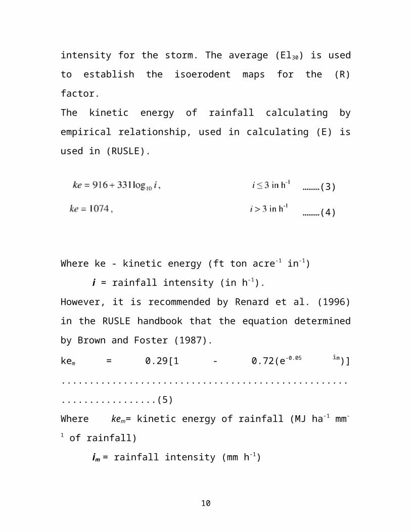
To compute the rainfall-runoff erosivity (R) factor in the (USLE) and
RUSLE is made by use of the (El30) parameter, where (E) is the total storm
energy and (I30) is the maximum 30-minute rainfall intensity for the storm.
The average (El30) is used to establish the isoerodent maps for the (R) factor.
6

The kinetic energy of rainfall calculating by empirical relationship, used in
calculating (E) is used in (RUSLE).
………(3)
………(4)
Where ke - kinetic energy (ft ton acre-1 in-1)
i = rainfall intensity (in h-1).
However, it is recommended by Renard et al. (1996) in the RUSLE
handbook that the equation determined by Brown and Foster (1987).
kem = 0.29[1 - 0.72(e-0.05 im)] ....................................................................(5)
Where kem= kinetic energy of rainfall (MJ ha-1 mm-1 of rainfall)
im = rainfall intensity (mm h-1)
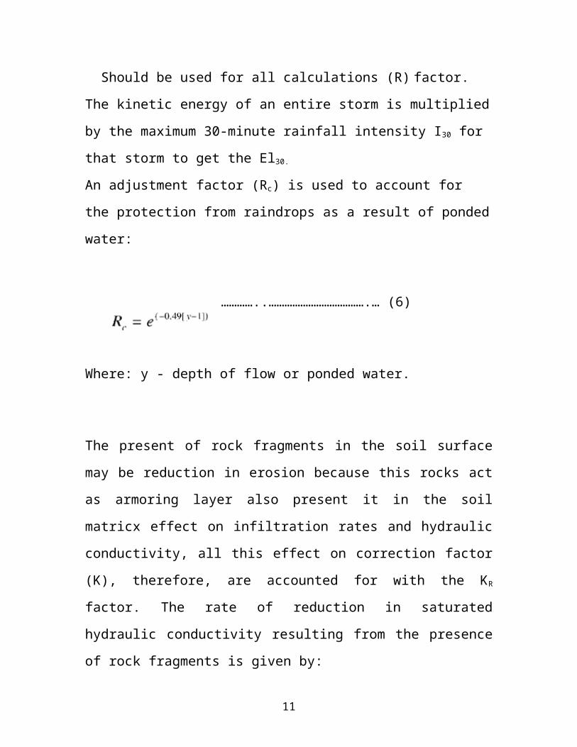
Should be used for all calculations (R) factor. The kinetic energy of an
entire storm is multiplied by the maximum 30-minute rainfall intensity I30
for that storm to get the El30.
An adjustment factor (Rc) is used to account for the protection from
raindrops as a result of ponded water:
…………..……………………………….… (6)
Where: y - depth of flow or ponded water.
7

The present of rock fragments in the soil surface may be reduction in erosion
because this rocks act as armoring layer also present it in the soil matricx
effect on infiltration rates and hydraulic conductivity, all this effect on
correction factor (K), therefore, are accounted for with the KR factor. The
rate of reduction in saturated hydraulic conductivity resulting from the
presence of rock fragments is given by:
………………………………………………(7)
Where: Kb - saturated hydraulic conductivity of the soil with rock fragments,
Kf = saturated hydraulic conductivity of the fine fraction of soil, and
Rw= percentage by weight of rock fragments > 2 mm.
The rock fragment decrease the saturated hydraulic conductivity of the
soil which is leading to increase of the soil erosion, the seasonal effects
such as freezing, soil texture and soil water also effect on (K) factor. The
melt of soil freezing increase the soil erodibility (K) factor because the
freeze changing many soil properties such as bulk density, soil structure,
hydraulic conductivity, soil strength and aggregate stability. The occurrence
of many freeze thaw cycles will tend to increase the (K) factor, while the
value of the soil erodibility factor will tend to decrease over the length of the
growing season in areas that are not prone to freezing periods. An average
annual value of (KR) is estimated from:
…………………………………………(8)
Where:- Eli - El.3o index at any time (calendar days).
8

……………………………………..(9)
Where Ki = soil erodibility factor at any time (ti in calendar days),Kmax - maximum soil erodibility factor at time tmax.
Kmin- minimum soil erodibility factor at time tmin.Δt - length of the frost-free period or growing period.
The slope length factor L is derived from plot data that indicate the
following relation:
…………………………………………………..……(10)
Where λ - horizontal projection of the slope length. 72.6 - RUSLE plot length in feet.
………………………………………………………(11)
Where β - ratio of rill to interrill erosion.
The value of (β) when the soil is moderately susceptible to rill and interrill erosion is given by:
…………………………….(12)
Where - slope angle.
The parameter (m) in the RUSLE is a function of (β) (Equation 11). The
newly defined (L) factor is combined with the original (S) factor to obtain a
new (LSR) factor. Values of (m) are in classes of low moderate, and high,
and tables are available in the RUSLE handbook for each of these classes to
obtain values for (LSR). Table 2.6 gives an example of the new (LSR) factor
values for soils with low rill erosion rates.
9
The all factors affect on soil loss erosion so the (USLE) becomes.
…………………………………………………….(13)
And the all factor (KR,CR,PR) must be calculated using the (RUSL, 1.06b program).
2.3- Modified Universal Soil Loss Equation.
Williams (1975) impose with no runoff yield no sediment with a little or no
rainfall and estimate the quantity with a single runoff event. He replaced
rainfall erosivity (R) with a runoff factor than the modified (USLE) is given
or (MUSLE) is given by the fallowing (Williams 1975).
10
Table (3) values of the topographic (LSR) factor for slopes with a low ratio of rill to interrill erosion( Renard et. al., 1996)
.................................................................... (14)
Where S - Sediment yield for a single event in tons.
Q - Total event runoff volume (ft').
pp= event peak discharge (ft3 s-1). .
K, LS, C, and P = USLE parameters (Equation 1).
The (MUSLE) can estimate soil loss from a single event, neither it nor the
(USLE and RUSLE) can estimate detachment, entrainment, transport,
deposition, and redistribution of sediment within the watershed and are of
limited application.
2.4- Direct Measurement of Sediment Yield and Extension of
Measured Data.
The best method for determining the amount of soil erosion from
watershed is by direct measurement of sediment deposition in reservoirs
(Blanton 1982) or by directed measurement for suspended load
concentration and bed load in the stream flow, the direct measurement needs
long time records are available. But the long-term measurements of river
discharge, suspended load and bed load are not commonly available.
However it may be possible to extend short-term measurements by empirical
correlation with records from another stream gauge in the watershed have
the similar drainage characteristics.
A short-term record of suspended sediment concentrations can be
extended by correlation with streamflow. A power equation of the form,
C = aQb ……………………………………………………………….(15)
11

This equation is most commonly used for regression analysis, where (C) is
the sediment concentration, Q is the rate of stream flow, and (a , b) are
regression coefficients.
The relationship between stream flow and suspended sediment
concentration can change with grain size, from low flows to high flows,
from season to season, and from year to year. For obtain a good result
enough measurements of suspended sediment concentration and stream flow
are necessary to ensure that the regression equation is applicable over a wide
range of stream flow conditions, seasons, and years. Strand (1975)
developed sediment yield equations as a function of drainage area based on
sediment survey data for Arizona, New Mexico, and California.
.................................................................................. (16)
Where Qs- sediment yield in ac-ft/mi2/yr
Ad - drainage area in mi2.
This same approach can be used to develop equations for other regions. If
the bedload measurements are not available, Strand and Pemberton (1982)
presented guide for estimating the ratio of the bedload to suspended load
(table 4) show that.
12
Table (4) bedload ratio to suspended load
3- Physically Based Approach for Erosion Estimates.
The energy dissipation in equilibrium dynamic system is minimum value
which is depends on the variables and condition of the system. The rate of
the energy dissipation per unit weight of water is.
Unit stream power = …………………… (17)
Where Y - potential energy per unit weight of water,
t- time. x - reach length,
dx/dt - velocity V. dY/dt - energy or water surface slope S.
The energy is dissipated by matieral transport and related with the rate of
material transported. Govers and Rauws (1986) proposed the relation
describe the relationship between stream power and many variables related
with sediment movement.
………………………………………………………….. (18)
Figure (2) showed relationship between unit stream power and sediment
concentration. Yang's (1973) original unit stream power equation was
intended for open channel flows. His dimensionless critical unit stream
power required at incipient motion may not be directly applicable to sheet
and rill flows. For sheet and rill flows with very shallow depth, Moore and
Burch found that the critical unit stream power required at incipient motion
can be approximated by a constant:
……………………………………………………(19)
13
The Yang(1973) unit stream power equation is a rational method based on
rainfall-runoff and unit stream power relationship can developed to replace
the empirical (USLE), because this theory can be used to determine the rate
of sediment transport in small and large rivers and it is possible use to
determine the total rate of sediment yield and transported from watershed
from compute the amount the sediment entering a reservoirs.
4- Computer Model Simulation of Surface Erosion Process.
Many computer models have been constructed to simulate soil erosion
within watershed area. These models can be grouped into several categories.
- Empirically based erosion models such as the USLE (Wischmeier and
Smith, 1978) and the RUSLE (Renard et al., 1996).
14
Fig.-2- Relationship between sheet and rill flow
sediment concentration unit stream power Govers
and Rauws (1986)
- Physically based models, such as the Water Erosion Prediction Project
(WEPP) (Nearing et al., 1989), Areal Non-point Source Watershed
Environmental Response Simulation (ANSWERS) (Beasley et al., 1980),
Chemicals, Runoff, and Erosion from Agricultural Management Systems
(CREAMS) (Kinsel, 1980), Kinematic runoff and Erosion model
(KINEROS) (Woolhiser et al., 1990), European Soil Erosion Model
(EUROSEM) (Morgan et al., 1998), and Systkme Hydrologique
Europken Sediment model (SHESED) (Wicks and Bathurst, 1996).
- Mixed empirical and physically based models, such as Cascade of Planes
in Two Dimensions (CASC2D) (Johnson et al., 2000; Ogden and Julien,
2002), Agricultural Non- Point Source Pollution model (AGNPS)
(Young et al., 1989), and Gridded Surface Subsurface Hydrological
Analysis model (GSSHA) (Downer, 2002).
- GIS and Remote Sensing techniques that utilize one of the previously listed
erosion models (Jiirgens and Fander, 1993; Sharma and Singh, 1995;
Mitasova et al., 2002).
Two dimensional models give more accurate result than one dimensional
models, but a little difference between them at predicting total sediment
yield (Hong and Mostaghimi 1997). Although the physically based models
give a good result , but it needs a lot of the parameters and that not
advisable to use a model in watershed area that does not have the requisite
data. The most important parameters for process-based models are rainfall
parameters (e.g., duration, intensity) and infiltration parameters (e.g.,
hydraulic conductivity).Poor quality input data can lead to large errors in
erosion modeling. Additionally, soil erosion models are built upon the
framework of hydrologic models that simulate the rainfall-runoff process.
15

Any error that exists in the hydrologic model will be propagated with the
error from the soil erosion model. However the error introduced from the
simulated runoff is generally much less than the error from the simulation of
erosion (Wu et al., 1993).
Due to the complexity of the surface erosion process, computer models are
needed for the simulation of the process and the estimation of the surface
erosion rate. These links below can be found many other soil erosion
models.
For describe and evaluate the performance of these models can be
return to the reference (Erosion and sedimentation manual).
4.1- Generalized Sediment Transport Model for Alluvial River
Simulation (GSTARS).
To simulate and predict the dynamic adjustment of channel and profile in
semi-three dimensional manner, use (GSTARS 2.1) model (Yang and
Simones, 2000). This model based on stream tube theory conjunction with
the theory of minimum energy dissipation rate or its simplified theory of
minimum of stream power. Fig.(3) show example to simulate and predict
geometry profile and compare with measured data. Also (Yang and Simoes,
2002) is an enhanced version of (GSTARS 2.1) to (GSTARS 3.0) for
simulate and predict the sedimentation processes in lakes and reservoirs. Fig.
(4) show example compare model result with the observed delta formation
(Swamee, 1974) in laboratory flume.
16
17
Fig.-3- Comparison of results produced by GSTARS 2.1 and survey data ( Yang and Simoes, 2000).
Fig.-4- Comparison of experiments with results produced by GSTARS 3.0 ( Yang and Simoes, 2000).

Also fig.(5) show the bed profile measured and predict by (GSTARS 3.0)
for Tarabela Reservoir in Pakistan ( Yang and Simoes, 2001), (GSTARS
3.0) and (GSTARS 2.1) enable us to simulate and predict the profile of river
system with all the processes that occurs within the system. For all cases
considering that the reservoirs, lakes and wetlands in watershed as a sink for
sediments.
18
Fig. -5- Comparison between measured and simulated bed profiles by GSTARS3.0 for the Tarbela Reservoir in Pakistan (Yang and Simoes, 2001).

4.2- Rainfall-Runoff Relationship. Surface run-off is very complexity phenomenon to determine should be
known characteristic rainfall and watershed. Once the surface run-off given
a sheet, rill and gully erosion rate of a watershed can be computed, many
computer models existing to simulate this phenomenon and some of them
also have certain abilities to simulate sheet erosion rates of watershed. These
models are based on the same approach for determination of erosion,
sediment transport and deposition in watershed. These models are
Precipitation-Runoff Modeling System (PRMS) by Leavesley et al. (1983)
and the Hydrological Simulation Program-FORTRAN (HSPF) by Johanson
et al. (1984). Further the input data include Input data include meteorologic,
hydrologic, snow, and watershed descriptions. The outputs are runoff
hydrographs, including maximum discharge, flow volume, and flow
duration. The schematic diagram of (PRMS) model shown in the fig.(6). The
output result can used to input information for sediment routing model such
as (GSTARS 2.1 and GSTARS 3.0).
4.3- GSTAR-W Model.
The surface erosion effect on the soil environment also reduces the
agricultural productivity of watershed. The United Nation Atomic energy
Agency has organized 5-year international effort to determine the surface
erosion. Using radio isotopes as tracers collect data from different region by
used GIS and other technology to test the (GSTARS 2.1 and GSTARS 3.0)
and calibrated (GSTARS-W) to simulate and predict the surface erosion as
well as river morphologic processes and deposition in reservoirs and lakes.
The Environmental Protection Agency (EPA) and other agencies used
integrated models to evaluate the impact on total maximum daily load of
19

sediment (TMPL) of sediment due to change of land use or other human
activities. Fig. (7) Show schematic of this.
20
Fig. -6- Flowchart of the PRMS model (Leavesley ct al.. 1993).
Fig. -7-. Sediment TMDL study and decision making flowchart.

4.4- Erosion Index Map.
The surface erosion is a big problem so that it is necessary locating index
maps to identify areas of erosion that occur and take remedial measures. It
has been observed that the unit stream power (vs/w) is the most important
parameter to determination the rate of erosion. From this construct the index
map thus we can put a preliminary estimation also may be modified this
index with green cover data (Gvs/w) by green cover factor and this it range
between 0 for paved surfaces and 1 for surfaces with no ground cover.
5- Reservoir Sedimentation.
All reservoir formed by dams on natural rivers, due to this the velocity
become very low so that the reservoir make as a trap for to deposition of
sediment in it this sediment is effect on the reservoir life. Then the useful life
of the reservoir might become very short. Therefore should be reducing
reservoir sedimentation. There are several methods available for reducing it.
These methods depend on the condition of the reservoir.
5.1- Reservoir Sediment Trap Efficiency.
Almost all sediment collected from watershed deposited within the
reservoirs. So the reservoir as considered trap for the sediment and the
efficiency is the ratio of the deposited sediment to the total sediment inflow.
It depends on many factors depend primarily upon the fall velocity, sediment
characteristic and velocity in the reservoir (Strand and Pemberton, 1982).
Also reservoir characteristic and operation system are affecting on the trap
efficiency, must be pointed out the important points in determining the
potential for reservoir sedimentation.
21

1- The reservoir storage capacity (at the normal pool elevation) relative to
the mean annual volume of river flow. This is used as an index the
reservoir sediment trap efficiency.
2- The average and maximum width of the reservoir relative to the average
and maximum width of the upstream river channel.
3- The average and maximum depth of the reservoir relative to the average
and maximum depth of the upstream river channel.
4- The purposes for which the dam and reservoir are to be constructed and
how the reservoir will be operated (e.g., normally full, frequently drawn
down, or normally empty).
5- The reservoir storage capacity relative to the mean annual sediment load
of the inflowing rivers.
6- The concentration of contaminants and heavy metals being supplied from
the upstream watershed.
Churchill (1948) developed dimensionless curve shows the relationship
between the percent of incoming sediment passing through the reservoir and
sediment index. Also in (1952) Brune proposed an empirical relationship for
estimating reservoir trap efficiency these shown in fig.(8). provides a good
comparison of the Brune and Churchill methods for computing trap
efficiencies using techniques developed by Murthy (1980). Burne method
use as a general guide line for large storage or normal ponded reservoirs and
Churchill curve for settling basin, small reservoirs, flood retarding
structures, semi-dry reservoirs. When the expected sediment accumulative
greater than (10%) of the reservoir capacity then should be analyzed the trap
efficiency for the additional periods of the reservoir life.
22

The estimated sediment inflow to reservoirs is very important to expect the
reservoir life (Strand and Pemberton, 1982). The mean annual sediment
inflow, the trap efficiency of the reservoir, the ultimate density of the
deposited sediment, and the distribution of the sediment within the reservoir
all must be considered in the design of the dam. To prevent the loss in the
reservoir storage capacity should be added the anticipated sediment
deposition volume during the life in the design (Strand and Pemberton,
1982). A 100-year period of economic analysis and sediment accumulation
was used for those reservoirs. Fig.(9) shows the effect of sediment on
storage capacity of reservoirs. However, the total sediment deposition is
used for design purposes to set the sediment elevation at the dam, to
determine loss of storage due to sediment in any assigned storage space, and
to help determine total storage requirements.
23
Fig.-8- Trap efficiency curves (Churchill, 1948; and Burne, 1952)
Fig. -9- Schematic diagram of anticipated sediment deposition (Bureau of Reclamation, 1987).

5.2- Density of Deposited Sediment.
The density of the sediment deposit in reservoirs measured in dry mass
per unit volume is used to converted the total sediment enter in reservoir
from mass to volume. The density of sediment deposited in the reservoirs
affected by.
1- The way of reservoirs operation. The influence of reservoir operation
is one of the most important factors because affect directly on the
consolidation or drying out that can occur in the clay fraction of
sediments deposited. Reservoirs operating with a constant stage yields
the same degree of consolidate.
2- Sediment size deposited.
3- Compact or consolidation rate of deposited sediment. the
new sediment deposits will change the density of the old sediment
deposits.
5.3- Sediment Distribution within a Reservoir.
24

In (1978) (U.S. Department of Agriculture) used data for different
reservoirs to develop empirical relationships for predicting sediment
distribution in reservoirs (Strand and Pemberton, 1982). Fig (10 and 11) is
the most common techniques for sediment distribution (U.S. Burea
reclamation, 1987) used data of (11) Great Plains reservoir in united state
that may be used as a guide in estimating the portion of total sediment
deposition within the reservoir.
25
Fig. -10-Sediment distribution from reservoir surveys of Lake Mead (Bureau of Reclamation, 1987)
Fig.-11- Sediment deposition profiles of several reservoirs (Bureau of Reclamation. 1987).
1- Empirical Area-Reduction method may be used to estimate the sediment
distribution, the method develop from data of (30) reservoirs. This method
described by Borland and Miller (1960) with revisions by Lara (1962). In
this method sediment distribution depends on.
The manner of reservoir operation.
Sediment size and shape.
Shape of the reservoir.
The amount of sediment.
The shape of reservoir regard the major criterion for development of
empirically derive designs curve for use in distributing sediment. Shown in
fig.(12). With equal weight applied to reservoir operation and shape. Weight
type distribution is select from table (5) in these cases where chose of two
types are given depend on the factor is more influential. Only for those cases
with two possible type distributions should be chose one size distribution but
26

the materials in most river systems is a mixture of clay, silt and sand
therefore the effect of size to be least important Lara (1962) provides the
detail on distributing sediment in reservoirs. The appropriate design type
curve is selected using the weighting procedure shown in table (5). Studies
have shown that a reservoir dose change type with sediment depositions.
Once a reservoir has been assigned a type by shape this classification will
not change. However it possible that a change in reservoir operation could
produce a new weighted type as defined in the same table.
2- The are increment method is suitable to the type (II) design curve and
based on the assumption that the area of sediment deposition remain
constant (Strand and Pemberton 1982) applied this method on Theodore
Roosevelt dam, located on the salt river in Arizona this method used to
predict the amount of sediment deposit in the future estimate the life of
reservoir and distribution of sediment.
5.4- Delta Deposits.
27

The flow velocity in the reservoirs decreases closer to the dam due to the
backwater flow so that the coarse material deposit away from the dam and
fine material near the dam as shown in fig.(12) and then cause rising of the
backwater elevation in the river (upstream from reservoir) cause more
deposit in the upstream due to decrease of flow velocity this phenomenon
called delta.
To predicting the delta within a reservoirs is complex problem because of
more variables are affect such as operation of reservoir, size of sediment and
hydraulics characteristic of river and reservoir. (Stand and Pemberton 1982)
proposed trail and error method empirical procedure. The method based on
the size of the sediment deposit in the delta is greater than (0.062mm), trial
and error method used the topographic data and volume computations by
average end-area method is used to arrived at final delta location. The delta
formation can also be determined from computer modeling, due to
developed computer technique modeling in the recent decades.
28
Fig.(12) Typical sediment deposition profile (Bureau of Reclamation, 1987)

5.5- Minimum Unit Stream Power and Minimum Stream
Power Method.
Yang (1971) presented the theory of minimum unit stream power. He
supposes that the system is closed and energy dissipated under dynamic
equilibrium.
………………………………….(20)
Where. Y - Potential energy per unit weight of water.
x – Distance. VS - Unit stream power.
V - Average flow velocity. S – Slope.
t - Time.
This value (VS) depends on system condition. Yang (1976) applied the
theory on fluvial system also Yang (1976) and Yang and Song (1986) derive
the theory of minimum energy dissipation rate from basic principle in fluid
mechanic and mathematic then called on it minimum energy dissipation rate.
These theories have been applied to solve a wide range of fluvial hydraulic
problems.
29
Recommended