Boyce/D
iPrim
a 9th
ed, C
h 7.3: S
ystems of L
inear
Eq
uation
s, Lin
ear Ind
epen
den
ce, Eigen
values
Elem
entary Differential E
quations and Boundary V
alue Problem
s, 9thedition, by W
illiam E
. Boyce and R
ichard C. D
iPrim
a, ©2009 by John W
iley & S
ons, Inc.
A system
of nlinear equations in n
variables,
can be expressed as a matrix equation A
x=
b:
If b=
0, then system is h
omogen
eous; otherw
ise it is n
onh
omogen
eous.
nn
nn
nn
n n
b b b
x x x
aa
a
aa
a
aa
a
2 1
2 1
,2,
1,
,22,
21,
2
,12,
11,
1
,,
22,
11,
2,2
22,
21
1,2
1,1
22,
11
1,1
nn
nn
nn
nn
nn
bx
ax
ax
a
bx
ax
ax
a
bx
ax
ax
a
Nonsingular C
ase
If the coefficient matrix A
is nonsingular, then it is invertible and w
e can solve Ax
= b
as follows:
This solution is therefore unique. A
lso, if b=
0, it follows
that the unique solution to Ax
= 0
is x=
A-10
= 0.
Thus if A
is nonsingular, then the only solution to Ax
= 0
is the trivial solution x
= 0.
bA
xb
AIx
bA
Ax
Ab
Ax
11
11
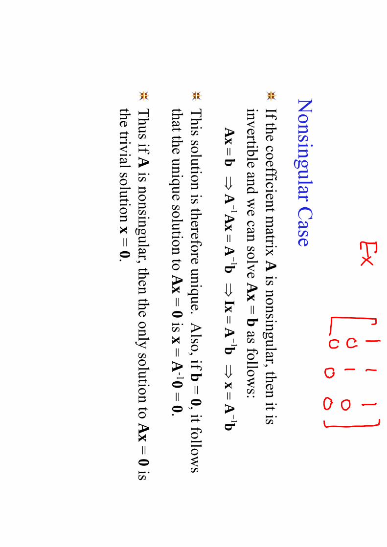
Exam
ple 1: Nonsingular C
ase (1 of 3)
From
a previous example, w
e know that the m
atrix Abelow
is nonsingular w
ith inverse as given.
Using the definition of m
atrix multiplication, it follow
s that the only solution of A
x=
0is x
= 0:
4/1
4/3
4/1
4/1
4/7
4/5
4/1
4/5
4/3
,
11
2
21
1
32
11
AA
0 0 0
0 0 0
4/1
4/3
4/1
4/1
4/7
4/5
4/1
4/5
4/3
10A
x
Exam
ple 1: Nonsingular C
ase (2 of 3)
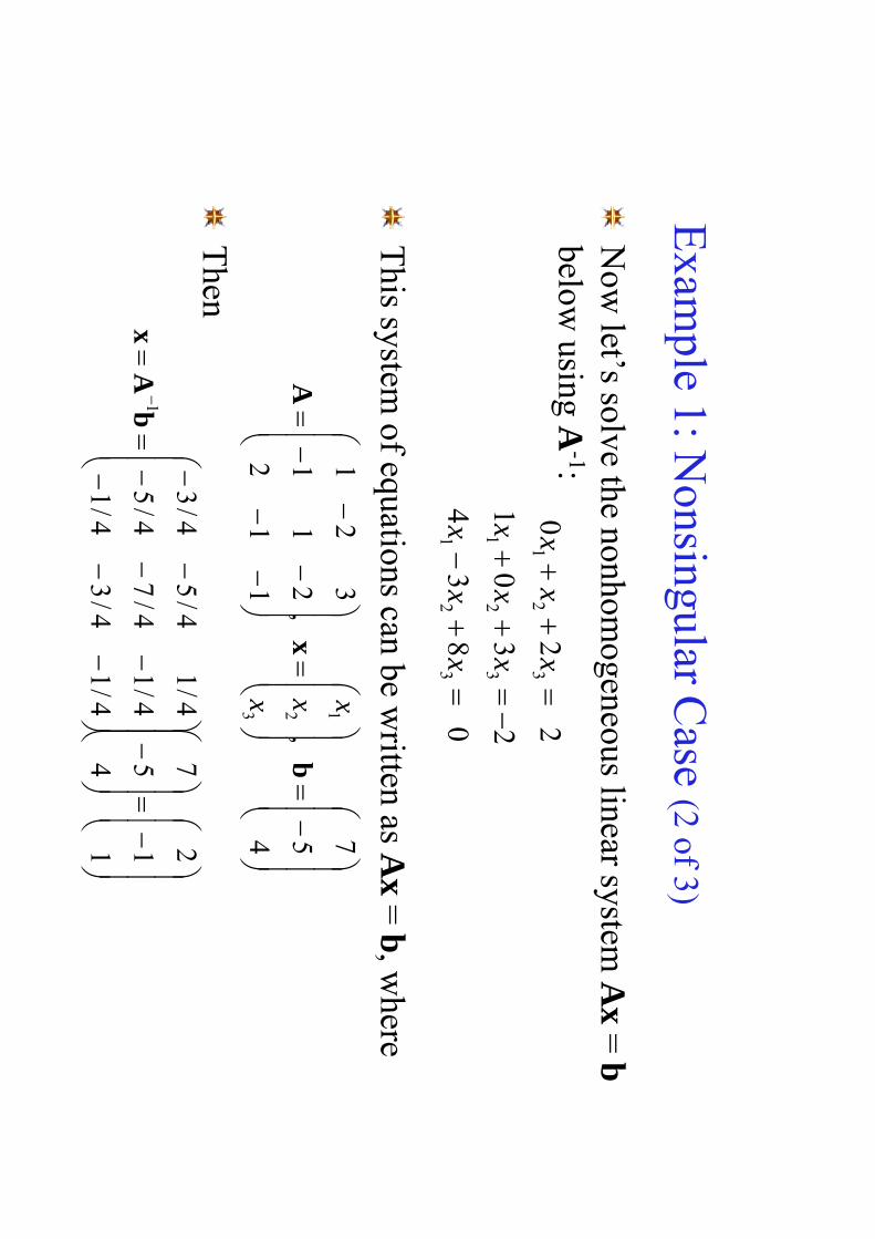
Now
let’s solve the nonhomogeneous linear system
Ax
= b
below using A
-1:
This system
of equations can be written as A
x=
b, where
Then
08
34
23
01
22
0
32
1
32
1
32
1
xx
x
xx
x
xx
x
1 1 2
4 5 7
4/1
4/3
4/1
4/1
4/7
4/5
4/1
4/5
4/3
1bA
x
4 5 7
,,
11
2
21
1
32
1
3 2 1
bx
A
x x x
Exam
ple 1: Nonsingular C
ase (3 of 3)
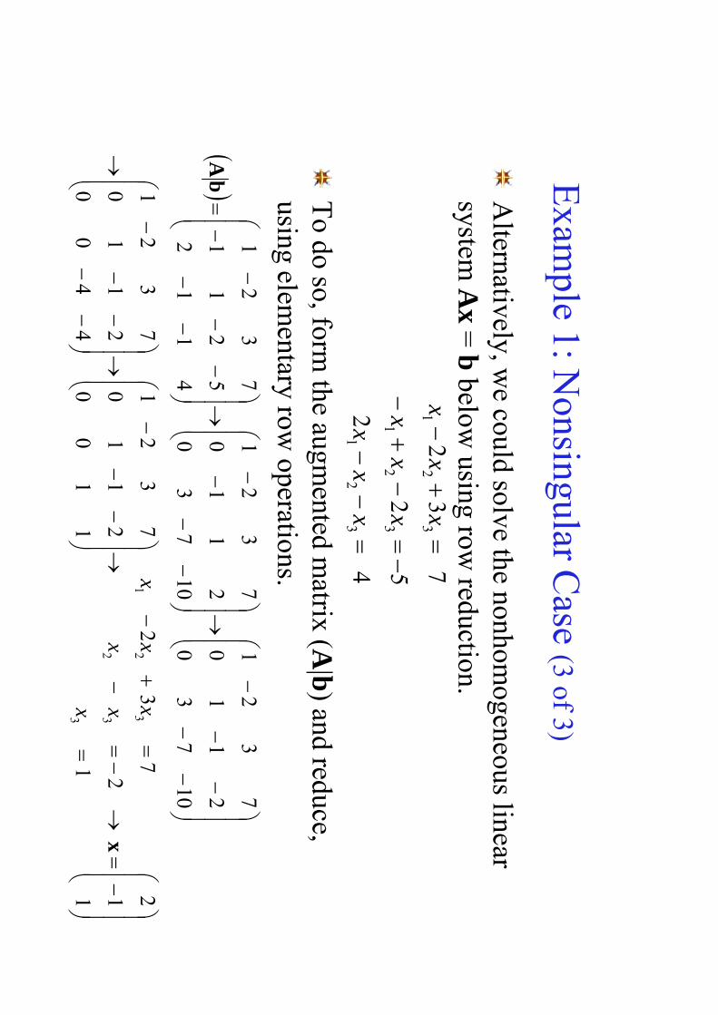
Alternatively, w
e could solve the nonhomogeneous linear
system A
x=
bbelow
using row reduction.
To do so, form
the augmented m
atrix (A|b
) and reduce, using elem
entary row operations.
1 1 2
1 2
73
2
11
00
21
10
73
21
44
00
21
10
73
21
107
30
21
10
73
21
107
30
21
10
73
21
41
12
52
11
73
21
3 32
32
1
x
bA
x xx
xx
x 42
52
73
2
32
1
32
1
32
1
xx
x
xx
x
xx
x

Singular C
ase
If the coefficient matrix A
is singular, then A-1
does not exist, and either a solution to A
x=
bdoes not exist, or there
is more than one solution (not unique).
Further, the hom
ogeneous system A
x=
0has m
ore than one solution. T
hat is, in addition to the trivial solution x=
0, there
are infinitely many nontrivial solutions.
The nonhom
ogeneous case Ax
= b
has no solution unless (b
, y) = 0, for all vectors y
satisfying A*y
= 0, w
here A*
is the adjoint of A
.
In this case, Ax
= b
has solutions (infinitely many), each of
the form x
= x
(0)+ , w
here x(0)is a particular solution of
Ax
= b
, and is any solution of A
x=
0.
Exam
ple 2: Singular C
ase (1 of 2)
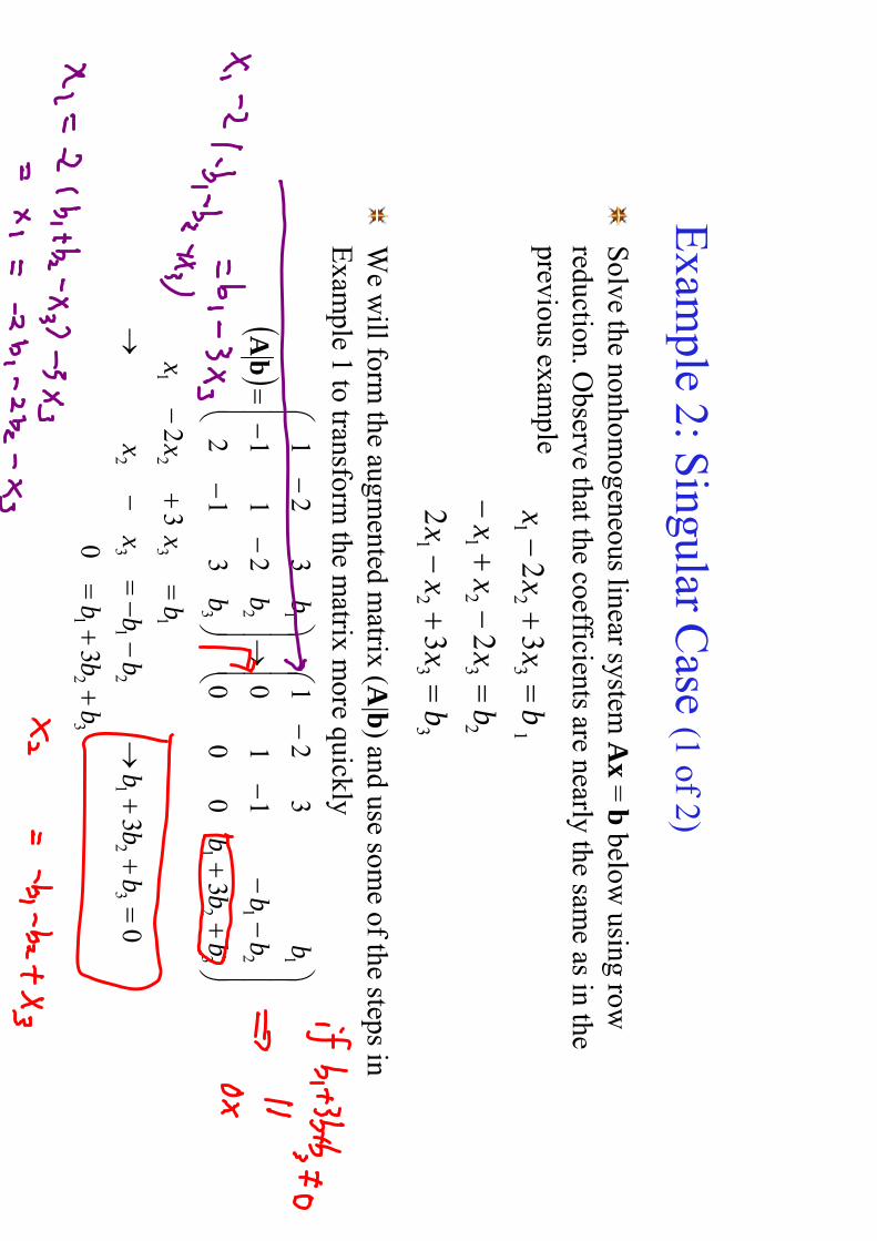
Solve the nonhom
ogeneous linear system A
x=
bbelow
using row
reduction. Observe that the coefficients are nearly the sam
e as in the previous exam
ple
We w
ill form the augm
ented matrix (A
|b) and use som
e of the steps in E
xample 1 to transform
the matrix m
ore quickly
03
30
32
30
00
11
0
32
1
31
2
21
1
32
1
32
1
32
1
21
32
13
21
32
1
21
1
3 2 1
bb
b
bb
b
bb
xx
bx
xx
bb
b
bb
b
b b b
bA
33
21
23
21
13
21
32
2 32
bx
xx
bx
xx
bx
xx
Exam
ple 2: Singular C
ase (2 of 2)
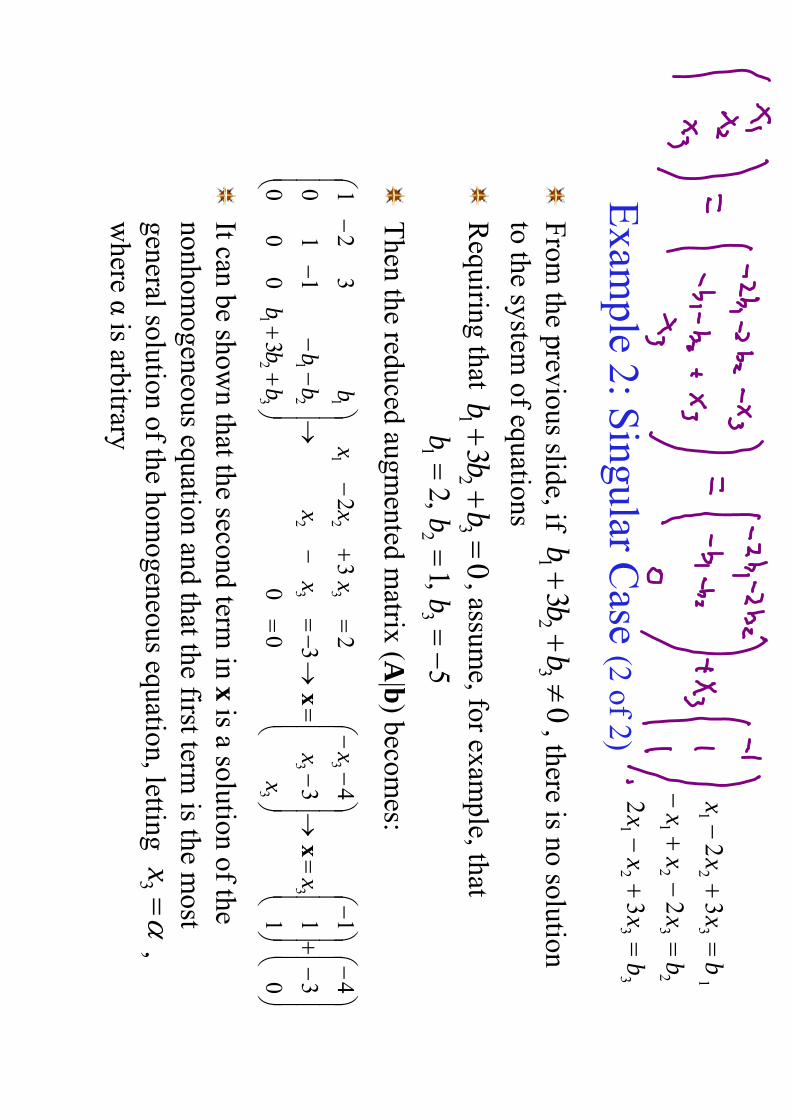
From
the previous slide, if , there is no solution
to the system of equations
Requiring that
, assume, for exam
ple, that
Then the reduced augm
ented matrix (A
|b) becom
es:
It can be shown that the second term
in xis a solution of the
nonhomogeneous equation and that the first term
is the most
general solution of the homogeneous equation, letting
, w
here αis arbitrary
0 3 4
1 1 1
3 4
00
3 23
2
30
00
11
0
32
1
3
3
3 3
32
32
1
32
1
21
1
x
x
x x
xx
xx
x
bb
b
bb
b
xx 0
33
21
b
bb
5,1
,23
21
bb
b0
33
21
b
bb
33
21
23
21
13
21
32
2 32
bx
xx
bx
xx
bx
xx
3
x
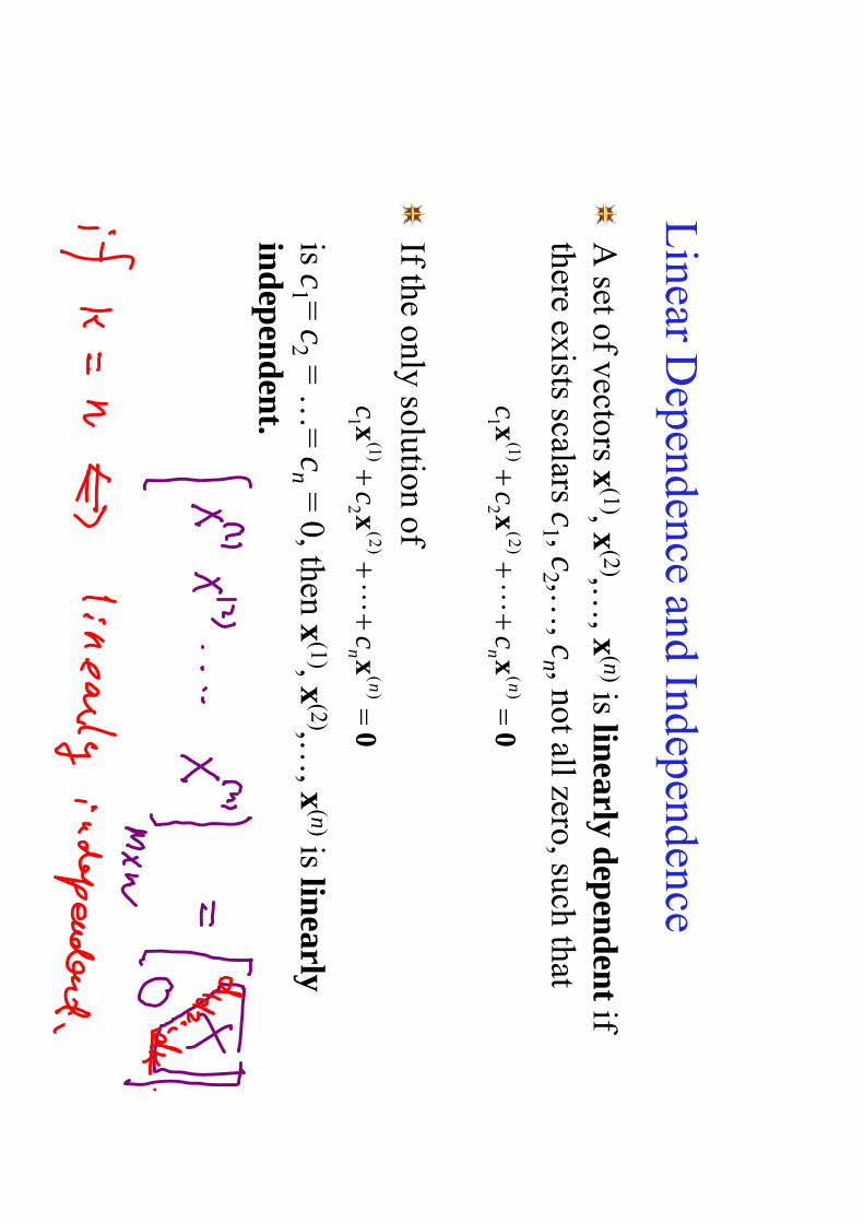
Linear D
ependence and Independence
A set of vectors x
(1), x(2),…
, x(n)is lin
early dep
end
ent
if there exists scalars c
1 , c2 ,…
, cn , not all zero, such that
If the only solution of
is c1 =
c2
= …
= c
n=
0, then x(1), x
(2),…, x
(n)is linearly
ind
epen
den
t.
0x
xx
)(
)2(
2)1
(1
nn
cc
c
0x
xx
)(
)2(
2)1
(1
nn
cc
c
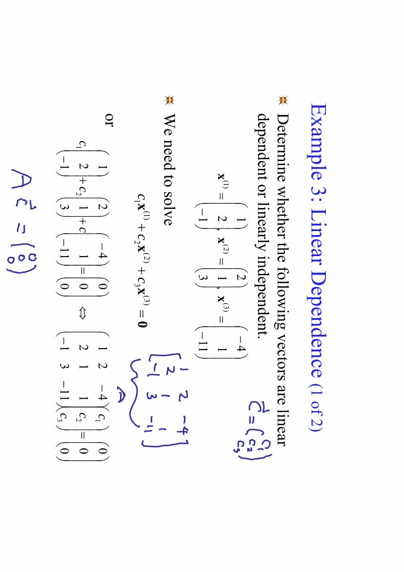
Exam
ple 3: Linear D
ependence (1 of 2)
Determ
ine whether the follow
ing vectors are linear dependent or linearly independent.
We need to solve
or
0 0 0
113
1
11
2
42
1
0 0 0
11 1 4
3 1 2
1 2 1
3 2 1
21
c c c
cc
c
0x
xx
)3
(3
)2(
2)1
(1
cc
c
11 1 4
,
3 1 2
,
1 2 1)3
()
2()1
(x
xx
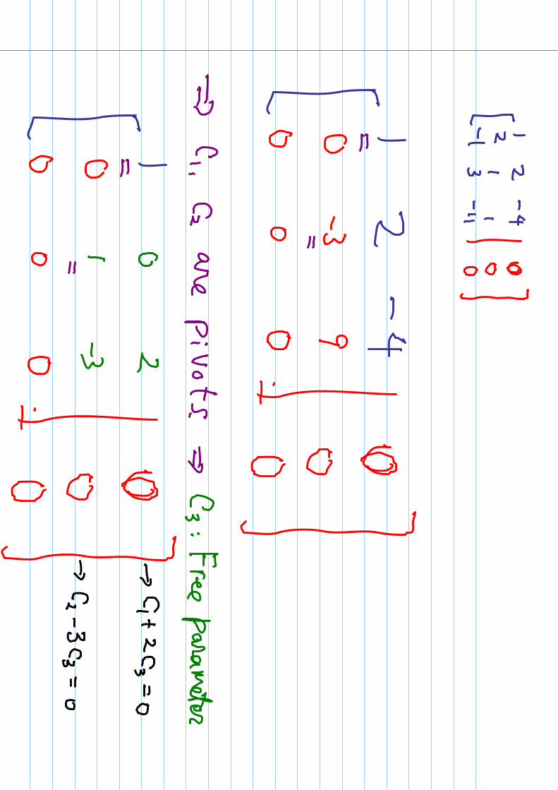

Exam
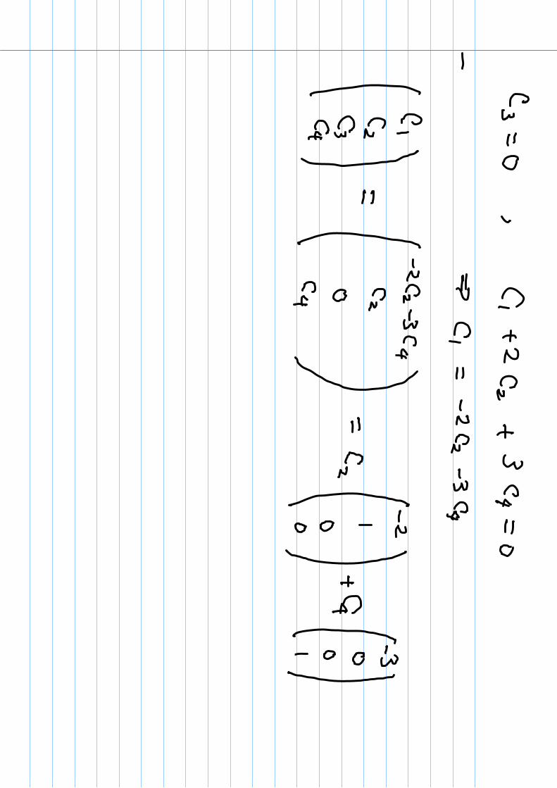
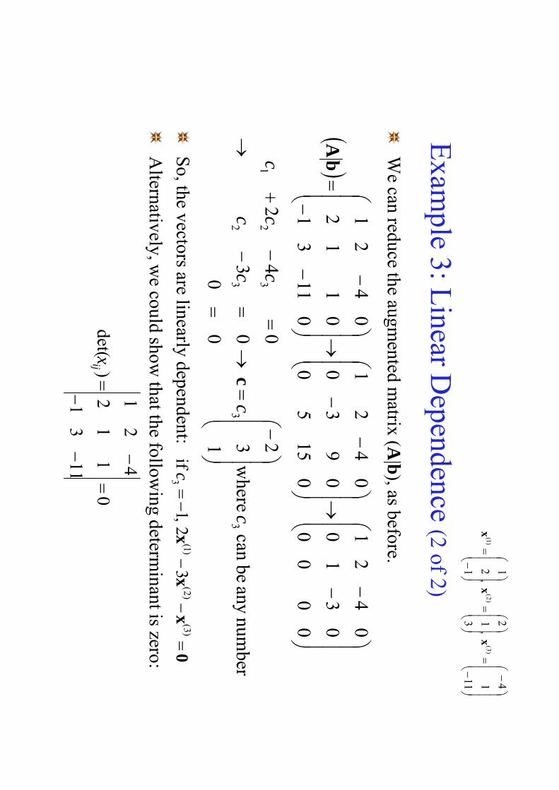
ple 3: Linear D
ependence (2 of 2)
We can reduce the augm
ented matrix (A
|b), as before.
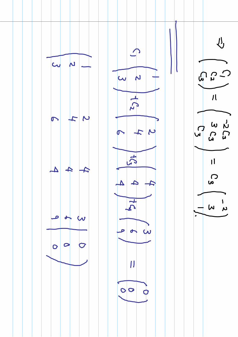
So, the vectors are linearly dependent:
Alternatively, w
e could show that the follow
ing determinant is zero:
number
any
becan
w
here
1 3 2
00
03
04
2
00
00
03
10
04
21
015
50
09
30
04
21
011
31
01
12
04
21
33
32
32
1
cc
cc
cc
c
c
bA
11 1 4
,
3 1 2
,
1 2 1)3
()
2()1
(x
xx
0
113
1
11
2
42
1
)det(
ijx
0x
xx
)3
()2
()1
(3
32,
1ifc
Linear Independence and Invertibility
Consider the previous tw
o examples:
The first m
atrix was know
n to be nonsingular, and its column vectors
were linearly independent.
The second m
atrix was know
n to be singular, and its column vectors
were linearly dependent.
This is true in general: the colum
ns (or rows) of A
are linearly independent iff A
is nonsingular iff A-1
exists.
Also, A
is nonsingular iff detA
0, hence columns (or row
s) of A
are linearly independent iff detA
0.
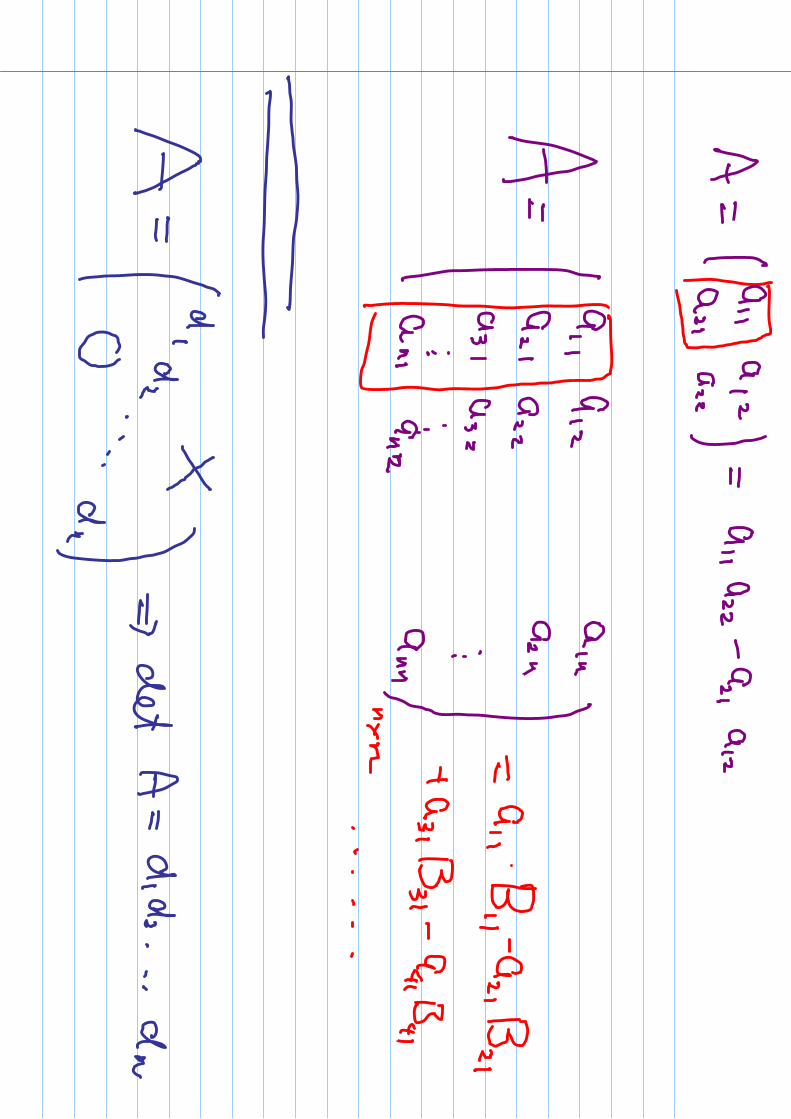
Further, if A
= B
C, then det(C
) = det(A
)det(B). T
hus if the colum
ns (or rows) of A
and Bare linearly independent, then
the columns (or row
s) of Care also.


Linear D
ependence & V
ector Functions
Now
consider vector functions x(1)(t), x
(2)(t),…, x
(n)(t), where
As before, x
(1)(t), x(2)(t),…
, x(n)(t) is lin
early dep
end
ent
on Iif
there exists scalars c1 , c
2 ,…, c
n , not all zero, such that
Otherw
ise x(1)(t), x
(2)(t),…, x
(n)(t) is linearly in
dep
end
ent
on I
See text for m
ore discussion on this.
,
,,
,2,1
,
)(
)(
)(
)(
)(
)(2
)(1
I
tn
k
tx
tx
tx
t
km k k
k
x
It
tc
tc
tc
nn
allfor
,)
()
()
()
()2
(2
)1(
10
xx
x
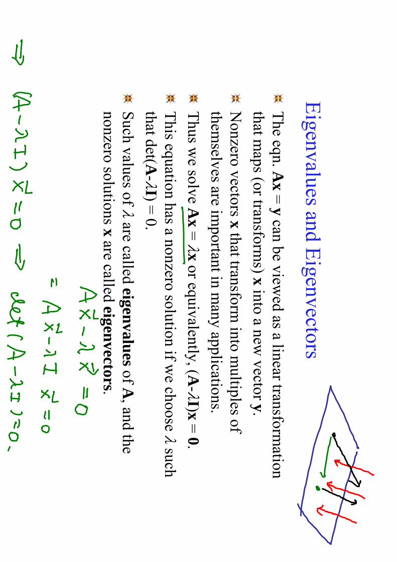
Eigenvalues and E
igenvectors
The eqn. A
x=
ycan be view
ed as a linear transformation
that maps (or transform
s) xinto a new
vector y.
Nonzero vectors x
that transform into m
ultiples of them
selves are important in m
any applications.
Thus w
e solve Ax
= x
or equivalently, (A-I)x
= 0.
This equation has a nonzero solution if w
e choose such
that det( A-I) =
0.
Such values of
are called eigenvalu
esof A
, and the nonzero solutions x
are called eigenvectors.
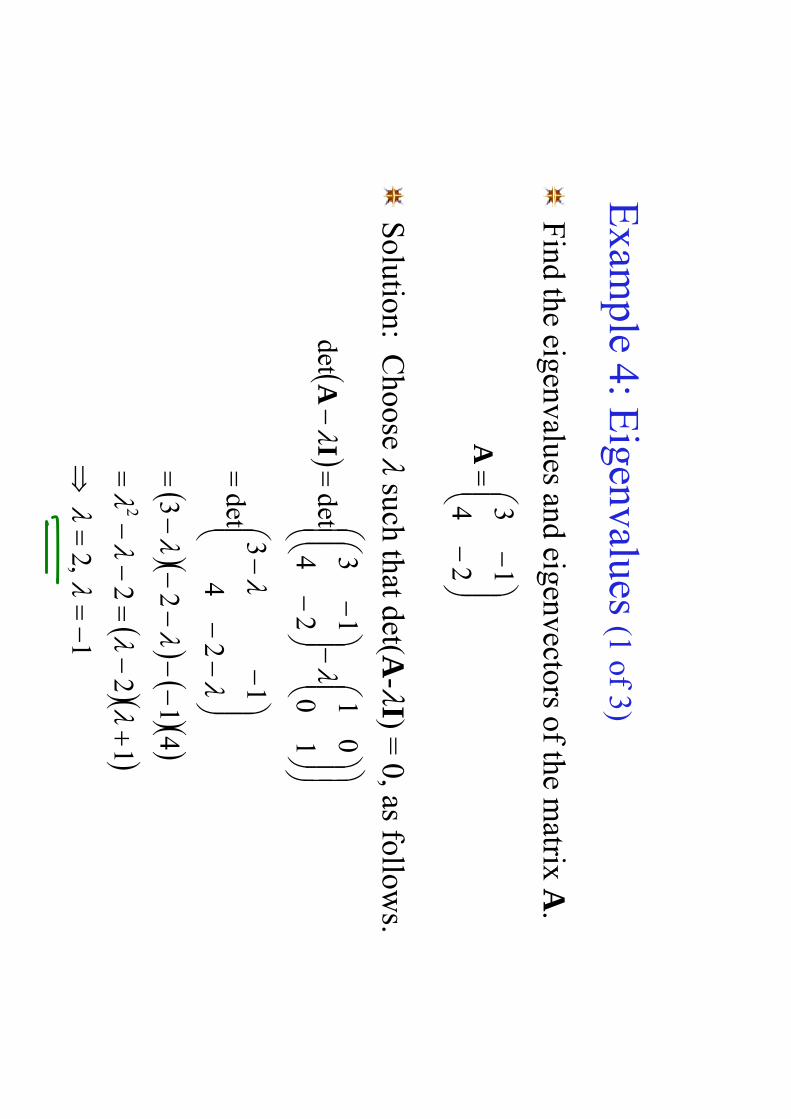
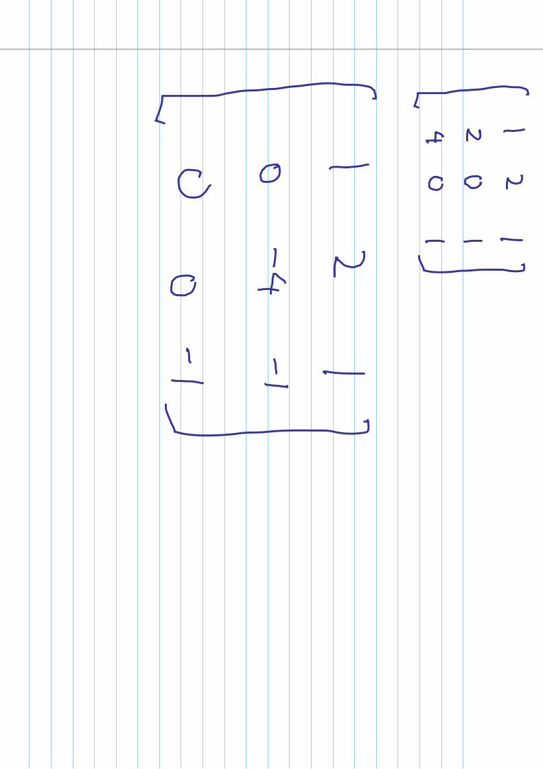
Exam
ple 4: Eigenvalues (1 of 3)
Find the eigenvalues and eigenvectors of the m
atrix A.
Solution: C
hoose such that det(A
-I) = 0, as follow
s.
24
13
A
1
,2
12
2
41
23
24
13
det
10
01
24
13
detdet
2
IA

Exam
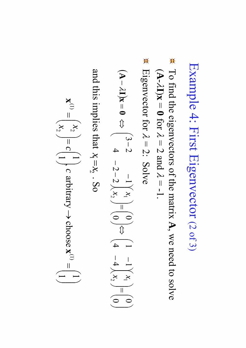
ple 4: First E
igenvector (2 of 3)
To find the eigenvectors of the m
atrix A, w
e need to solve ( A
-I)x=
0 for =
2 and =
-1.
Eigenvector for
= 2: S
olve
and this implies that
. So
0 0
44
11
0 0
22
4
12
3
2 1
2 1
x x
x x0
xI
A
1 1
choose
arbitrary,
1 1)1
(
2 2)1
(x
xc
cx x
21
xx

Exam
ple 4: Second E
igenvector (3 of 3)
Eigenvector for
= -1: S
olve
and this implies that
. So
0 0
14
14
0 0
12
4
11
3
2 1
2 1
x x
x x0
xI
A
4 1
choosearbitrary
,4 1
4)2
(
1 1)2
(x
xc
cx x
12
4xx

Norm
alized Eigenvectors
From
the previous example, w
e see that eigenvectors are determ
ined up to a nonzero multiplicative constant.
If this constant is specified in some particular w
ay, then the eigenvector is said to be n
ormalized
.
For exam
ple, eigenvectors are sometim
es normalized by
choosing the constant so that || x|| = (x, x) ½
= 1.
Algebraic and G
eometric M
ultiplicity
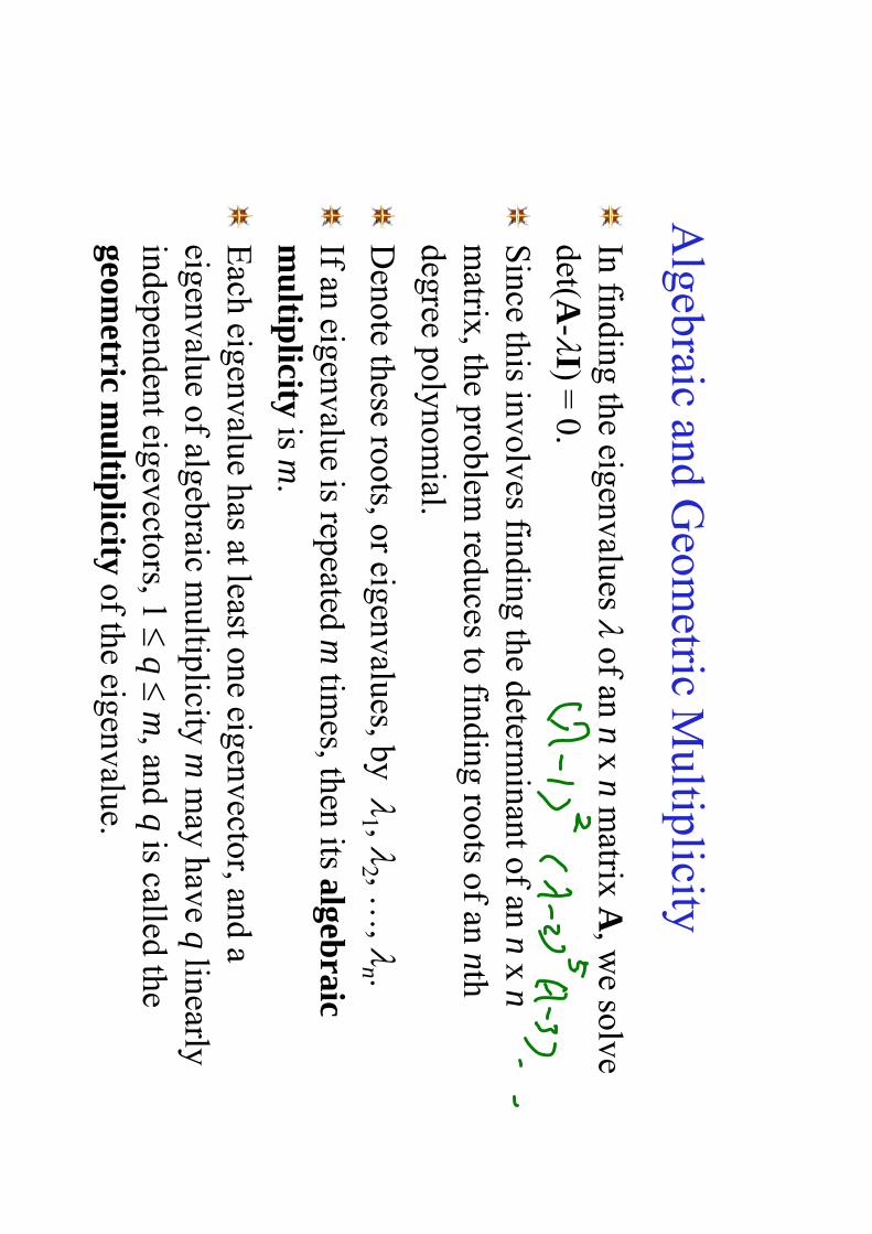
In finding the eigenvalues of an n
x nm
atrix A, w
e solvedet( A
-I) = 0.
Since this involves finding the determ
inant of an nx n
matrix, the problem
reduces to finding roots of an nth degree polynom
ial.
Denote these roots, or eigenvalues, by
1 , 2 , …
, n .
If an eigenvalue is repeated mtim
es, then its algebraic
mu
ltiplicity
is m.
Each eigenvalue has at least one eigenvector, and a
eigenvalue of algebraic multiplicity m
may have q
linearly independent eigevectors, 1
q m
, and qis called the
geometric m
ultip
licityof the eigenvalue.
Eigenvectors and L
inear Independence
If an eigenvalue has algebraic m
ultiplicity 1, then it is said to be sim
ple, and the geom
etric multiplicity is 1 also.
If each eigenvalue of an nx n
matrix A
is simple, then A
has ndistinct eigenvalues. It can be show
n that the neigenvectors corresponding to these eigenvalues are linearly independent.
If an eigenvalue has one or more repeated eigenvalues, then
there may be few
er than nlinearly independent eigenvectors
since for each repeated eigenvalue, we m
ay have q < m
. T
his may lead to com
plications in solving systems of
differential equations.
Exam
ple 5: Eigenvalues (1 of 5)
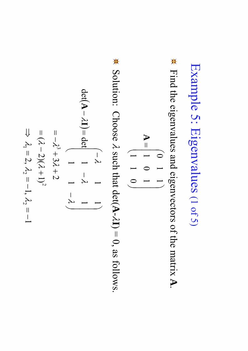
Find the eigenvalues and eigenvectors of the m
atrix A.
Solution: C
hoose such that det(A
-I) = 0, as follow
s.
01
1
10
1
11
0
A
1,1
,2
)1)(
2(
23
11
11
11
detdet
22
1
2
3
IA
Exam
ple 5: First E
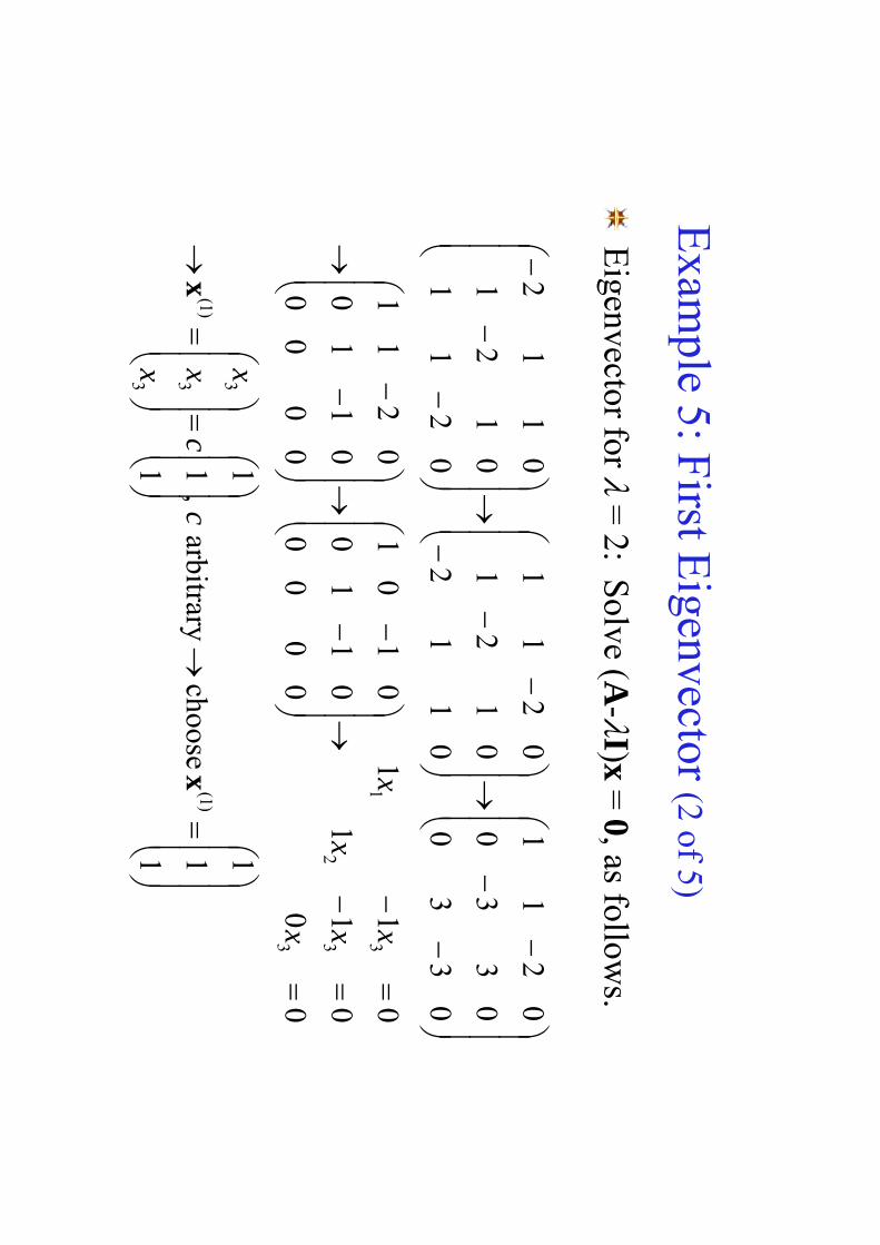
igenvector (2 of 5)
Eigenvector for
= 2: S
olve (A-I)x
= 0, as follow
s.
1 1 1
choose
arbitrary,
1 1 1
00
01
1
01
1
00
00
01
10
01
01
00
00
01
10
02
11
03
30
03
30
02
11
01
12
01
21
02
11
02
11
01
21
01
12
)1(
3 3 3)1
(
3 32
31
xx
cc
x x x
x xx
xx
Exam
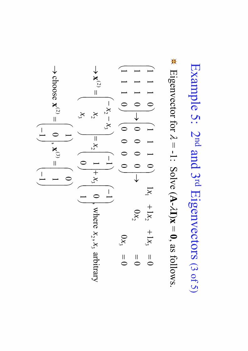
ple 5: 2nd
and 3rd
Eigenvectors (3 of 5)
Eigenvector for
= -1: S
olve (A-I)x
= 0, as follow
s.
1 1 0
,
1 0 1
choose
arbitrary,
where
,
1 0 1
0 1 1
00
00
01
11
00
00
00
00
01
11
01
11
01
11
01
11
)3(
)2(
32
32
3 2
32
)2(
3
2
32
1
xx
xx
xx
x
x x
xx
x
x
xx
x
Exam
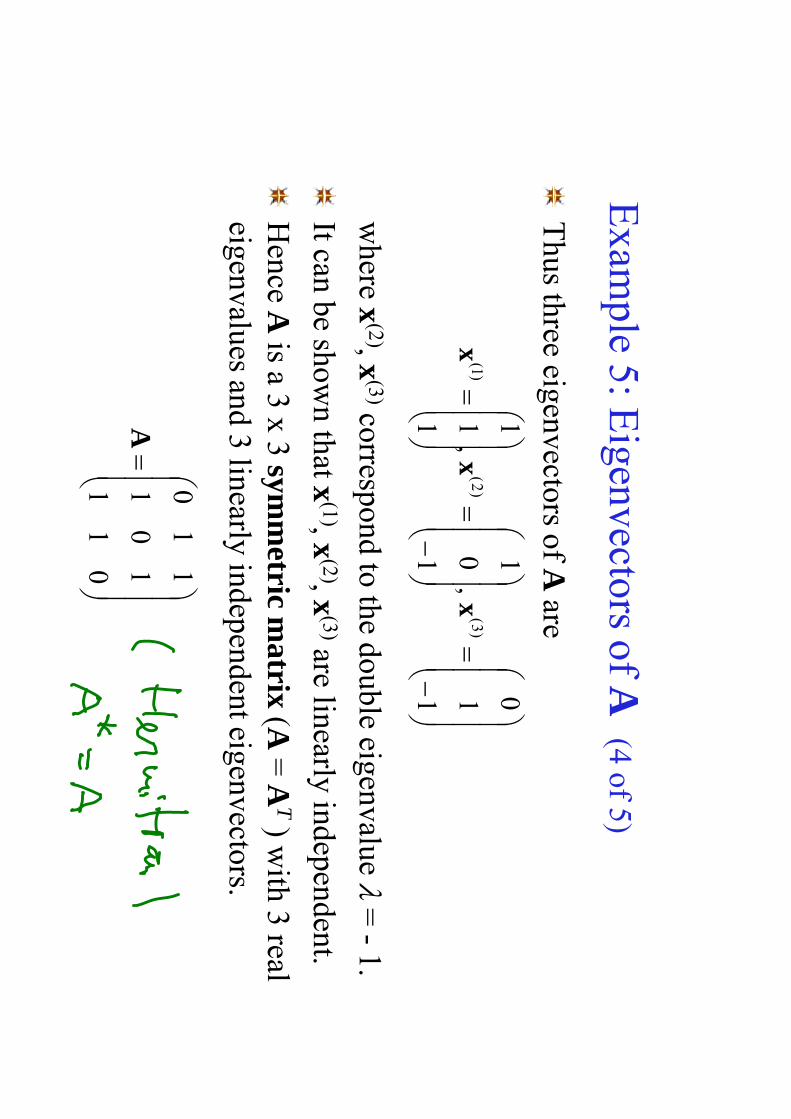
ple 5: Eigenvectors of A
(4 of 5)
Thus three eigenvectors of A
are
where x
(2), x(3)correspond to the double eigenvalue
= -
1.
It can be shown that x
(1), x(2), x
(3)arelinearly independent.
Hence A
is a 3 x 3 symm
etric matrix
(A=
AT
) with 3 real
eigenvalues and 3 linearly independent eigenvectors.
1 1 0
,
1 0 1
,
1 1 1)3
()2
()1
(x
xx
01
1
10
1
11
0
A
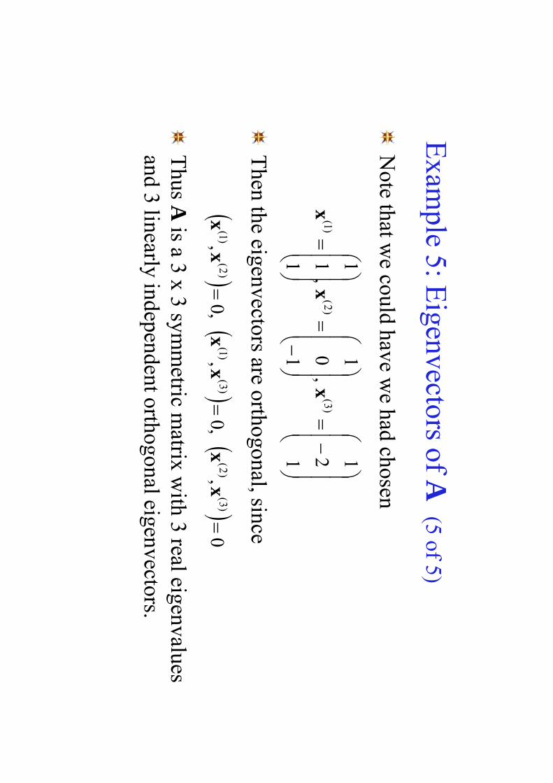
Exam
ple 5: Eigenvectors of A
(5 of 5)
Note that w
e could have we had chosen
Then the eigenvectors are orthogonal, since
Thus A
is a 3 x 3 symm
etric matrix
with 3 real eigenvalues
and 3 linearly independent orthogonal eigenvectors.
1 2 1
,
1 0 1
,
1 1 1)3
()2
()1
(x
xx
0
,,0
,,0
,)3
()2
()3
()1
()2
()1
(
xx
xx
xx
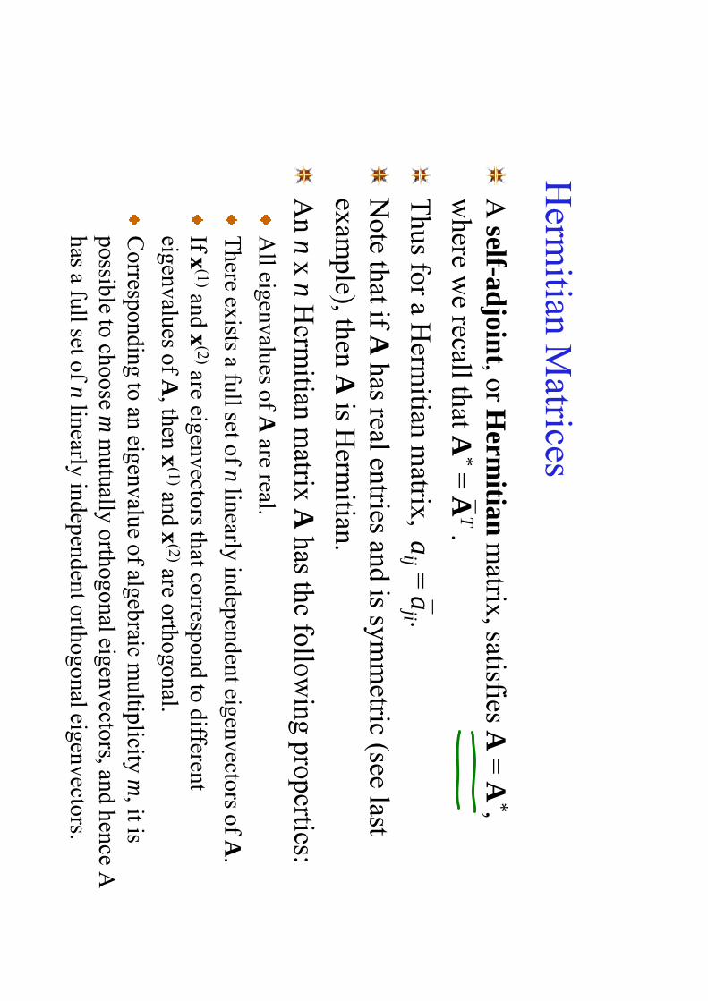
Herm
itian Matrices
A self-ad
joint, or H
ermitian
matrix, satisfies A
= A
*, w
here we recall that A
*=
AT
.
Thus for a H
ermitian m
atrix, aij =
aji .
Note that if A
has real entries and is symm
etric (see last exam
ple), then Ais H
ermitian.
An n
x nH
ermitian m
atrix Ahas the follow
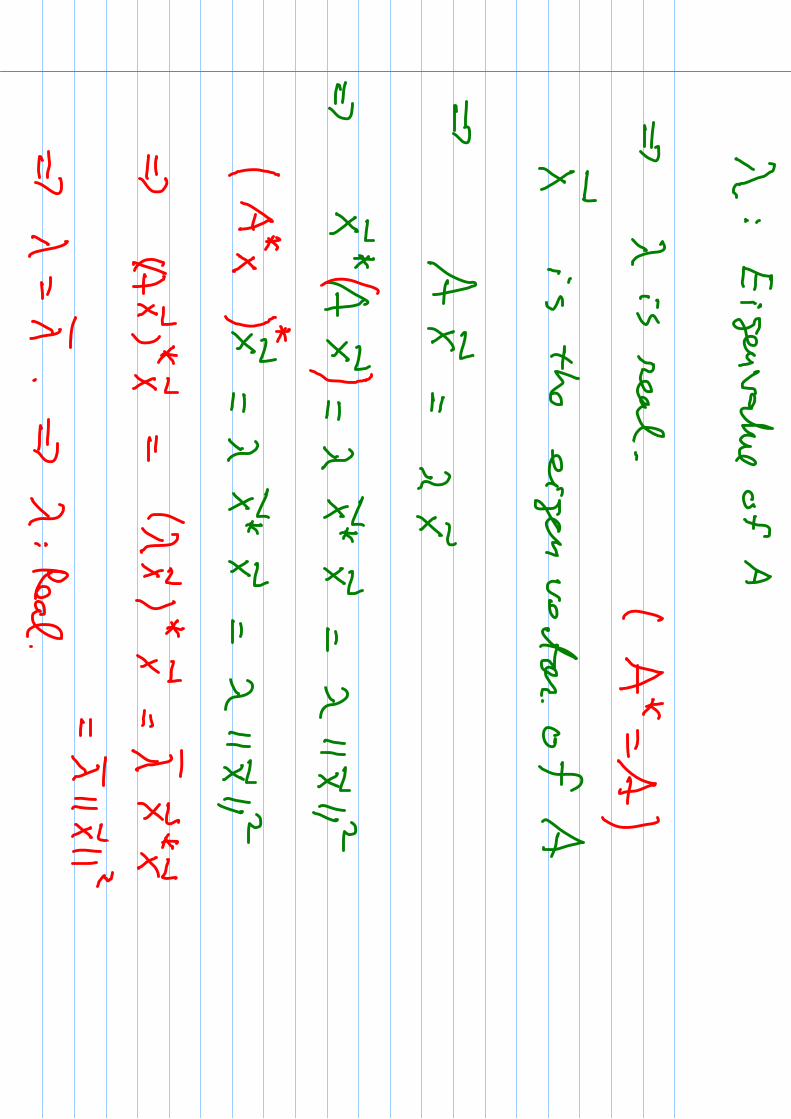
ing properties:A
ll eigenvalues of Aare real.
There exists a full set of n
linearly independent eigenvectors of A.
If x(1)and x
(2)areeigenvectors that correspond to different
eigenvalues of A, then x
(1)and x(2)are
orthogonal.
Corresponding to an eigenvalue of algebraic m
ultiplicity m, it is
possible to choose mm
utually orthogonal eigenvectors, and hence A
has a full set of nlinearly independent orthogonal eigenvectors.
Recommended