ENVE 576 Indoor Air Pollution Spring 2013 Lecture 2: January 22, 2013 Human exposure patterns Reactor models Ventilation and air exchange
Dr. Brent Stephens, Ph.D. Department of Civil, Architectural and Environmental Engineering
Illinois Institute of Technology [email protected]
Built Environment Research Group
www.built-envi.com Advancing energy, environmental, and sustainability research within the built environment
Review from last time
• Course overview • Introduction to indoor air
– Topics – Research – Literature
• Some basic air fundamentals
• Quick! – What is 50 µg/m3 of NO2 in ppb at standard temperature and
pressure?
2
Today’s objectives
• Human exposure patterns – Inhalation and intake fractions
• Reactor models
• Ventilation and air exchange rates
3
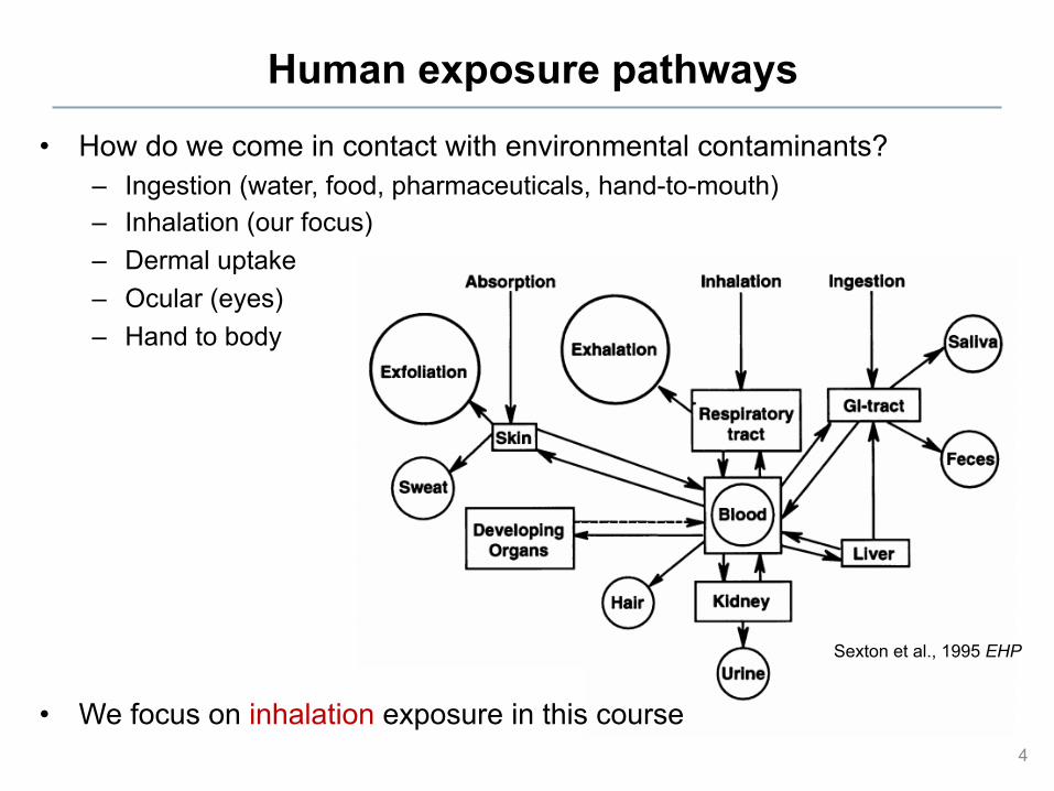
Human exposure pathways
• How do we come in contact with environmental contaminants? – Ingestion (water, food, pharmaceuticals, hand-to-mouth) – Inhalation (our focus) – Dermal uptake – Ocular (eyes) – Hand to body
• We focus on inhalation exposure in this course 4
Sexton et al., 1995 EHP
Inhalation exposure
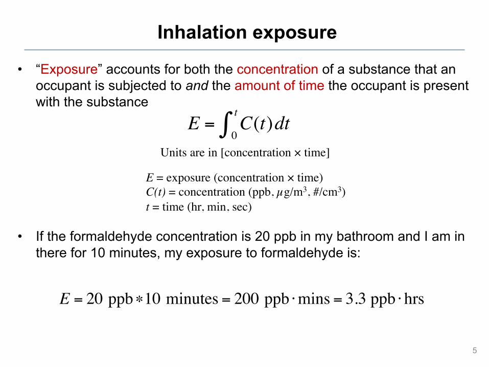
• “Exposure” accounts for both the concentration of a substance that an occupant is subjected to and the amount of time the occupant is present with the substance
• If the formaldehyde concentration is 20 ppb in my bathroom and I am in there for 10 minutes, my exposure to formaldehyde is:
5
E = 20 ppb!10 minutes = 200 ppb "mins = 3.3 ppb "hrs
E = C(t)dt0
t!
Units are in [concentration × time]
E = exposure (concentration × time) C(t) = concentration (ppb, µg/m3, #/cm3) t = time (hr, min, sec)
Inhalation exposure
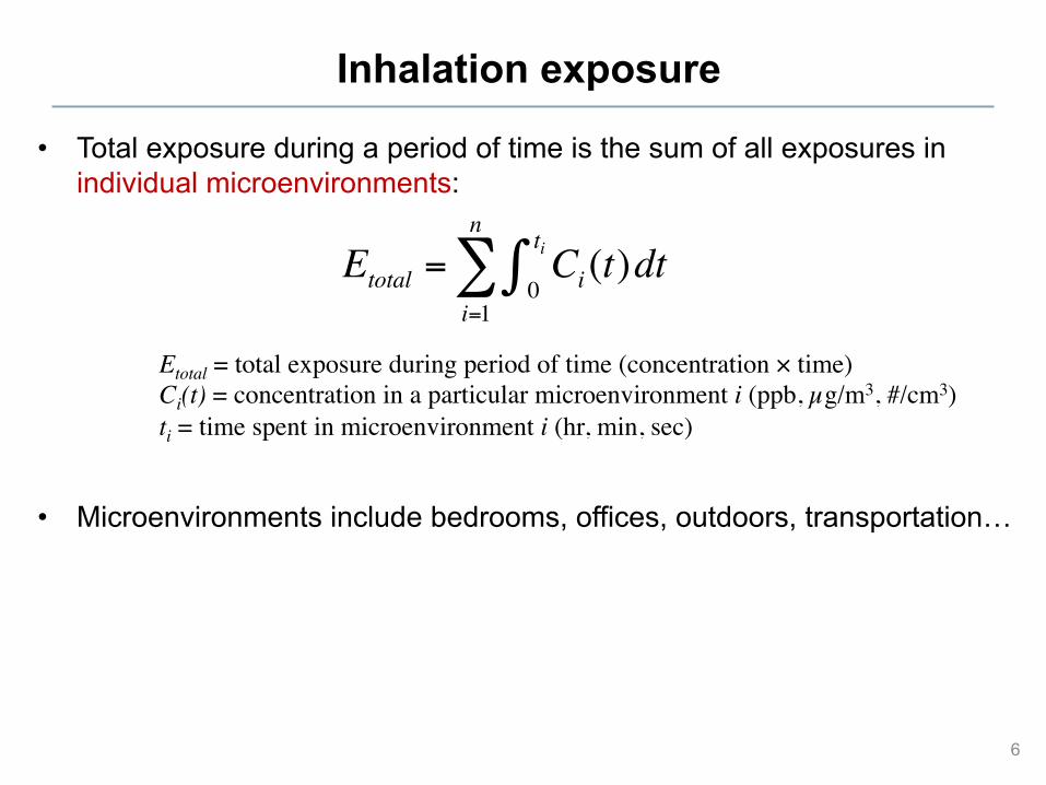
• Total exposure during a period of time is the sum of all exposures in individual microenvironments:
• Microenvironments include bedrooms, offices, outdoors, transportation…
6
Etotal = Ci (t)dt0
ti!i=1
n
"
Etotal = total exposure during period of time (concentration × time) Ci(t) = concentration in a particular microenvironment i (ppb, µg/m3, #/cm3) ti = time spent in microenvironment i (hr, min, sec)
Inhalation exposure
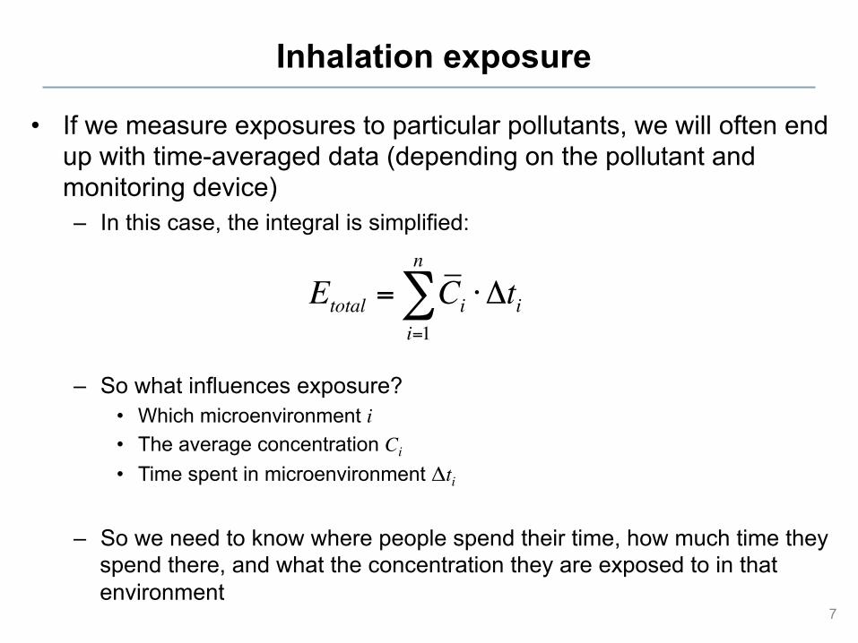
• If we measure exposures to particular pollutants, we will often end up with time-averaged data (depending on the pollutant and monitoring device) – In this case, the integral is simplified:
– So what influences exposure? • Which microenvironment i • The average concentration Ci
• Time spent in microenvironment Δti
– So we need to know where people spend their time, how much time they spend there, and what the concentration they are exposed to in that environment
7
Etotal = Ci ! "tii=1
n
#
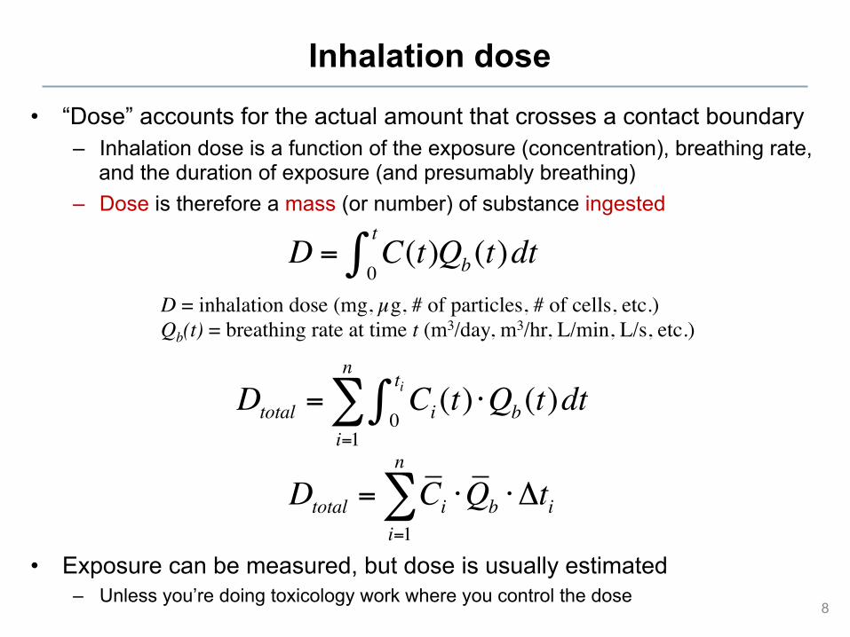
Inhalation dose • “Dose” accounts for the actual amount that crosses a contact boundary
– Inhalation dose is a function of the exposure (concentration), breathing rate, and the duration of exposure (and presumably breathing)
– Dose is therefore a mass (or number) of substance ingested
• Exposure can be measured, but dose is usually estimated – Unless you’re doing toxicology work where you control the dose
8
D = C(t)Qb(t)dt0
t!
Dtotal = Ci (t) !Qb(t)dt0
ti"i=1
n
#
Dtotal = Ci !Qb ! "tii=1
n
#
D = inhalation dose (mg, µg, # of particles, # of cells, etc.) Qb(t) = breathing rate at time t (m3/day, m3/hr, L/min, L/s, etc.)
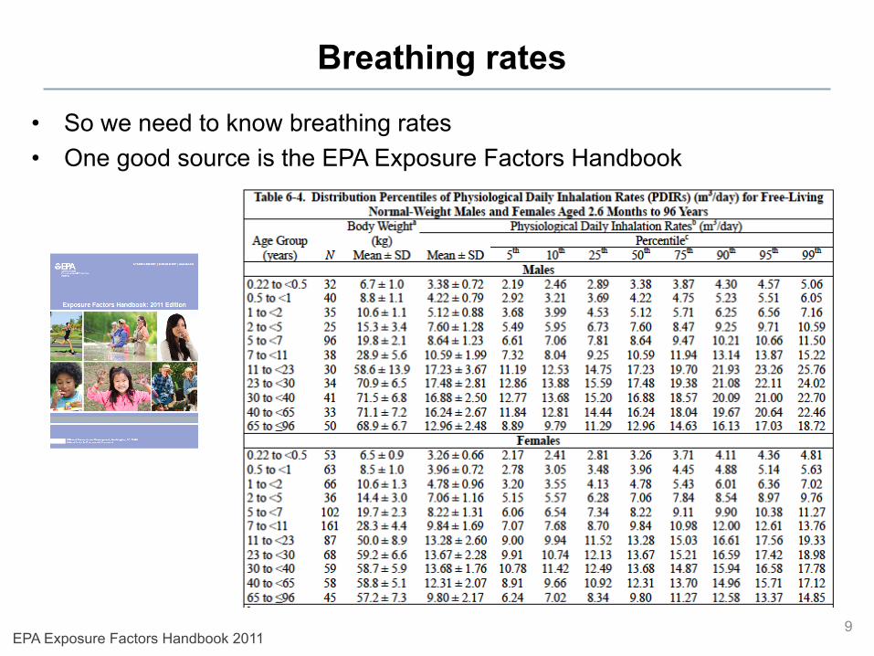
Breathing rates
• So we need to know breathing rates • One good source is the EPA Exposure Factors Handbook
9 EPA Exposure Factors Handbook 2011
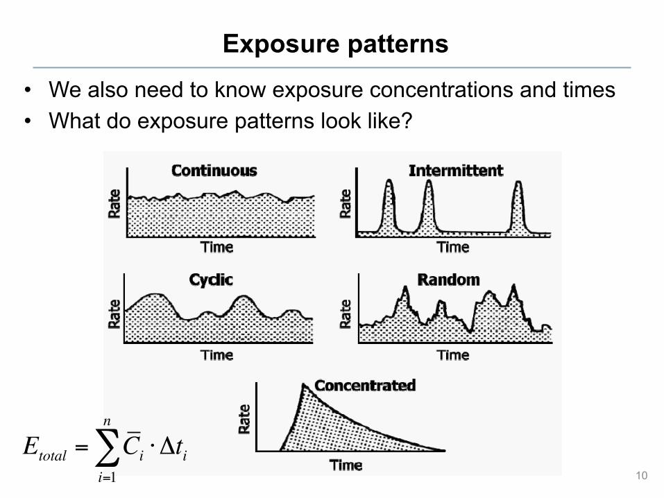
Exposure patterns
10
• We also need to know exposure concentrations and times • What do exposure patterns look like?
Etotal = Ci ! "tii=1
n
#
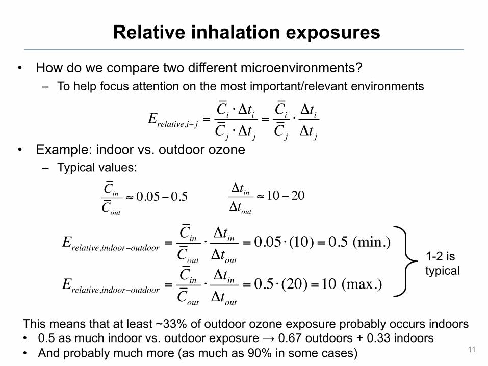
Relative inhalation exposures
• How do we compare two different microenvironments? – To help focus attention on the most important/relevant environments
• Example: indoor vs. outdoor ozone – Typical values:
11
Erelative,i! j =Ci " #tiCj " #t j
=Ci
Cj
"#ti#t j
Erelative,indoor!outdoor =Cin
Cout
"#tin#tout
= 0.05 " (10) = 0.5 (min.)
Erelative,indoor!outdoor =Cin
Cout
"#tin#tout
= 0.5 " (20) =10 (max.)
Cin
Cout
! 0.05" 0.5!tin!tout
"10# 20
1-2 is typical
This means that at least ~33% of outdoor ozone exposure probably occurs indoors • 0.5 as much indoor vs. outdoor exposure → 0.67 outdoors + 0.33 indoors • And probably much more (as much as 90% in some cases)
Human activity patterns
• So we need to understand where we spend our time in order to understand what exposures are important – Δti
• Where do we spend our time?
12
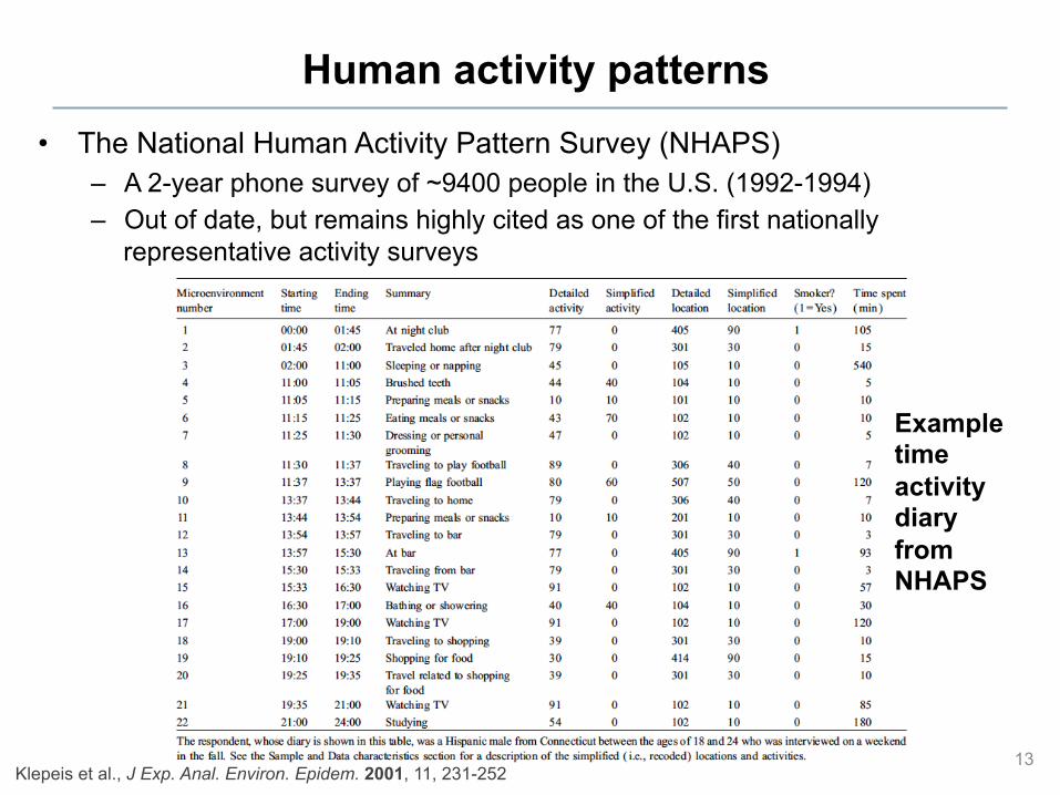
Human activity patterns • The National Human Activity Pattern Survey (NHAPS)
– A 2-year phone survey of ~9400 people in the U.S. (1992-1994) – Out of date, but remains highly cited as one of the first nationally
representative activity surveys
13 Klepeis et al., J Exp. Anal. Environ. Epidem. 2001, 11, 231-252
Example time activity diary from NHAPS
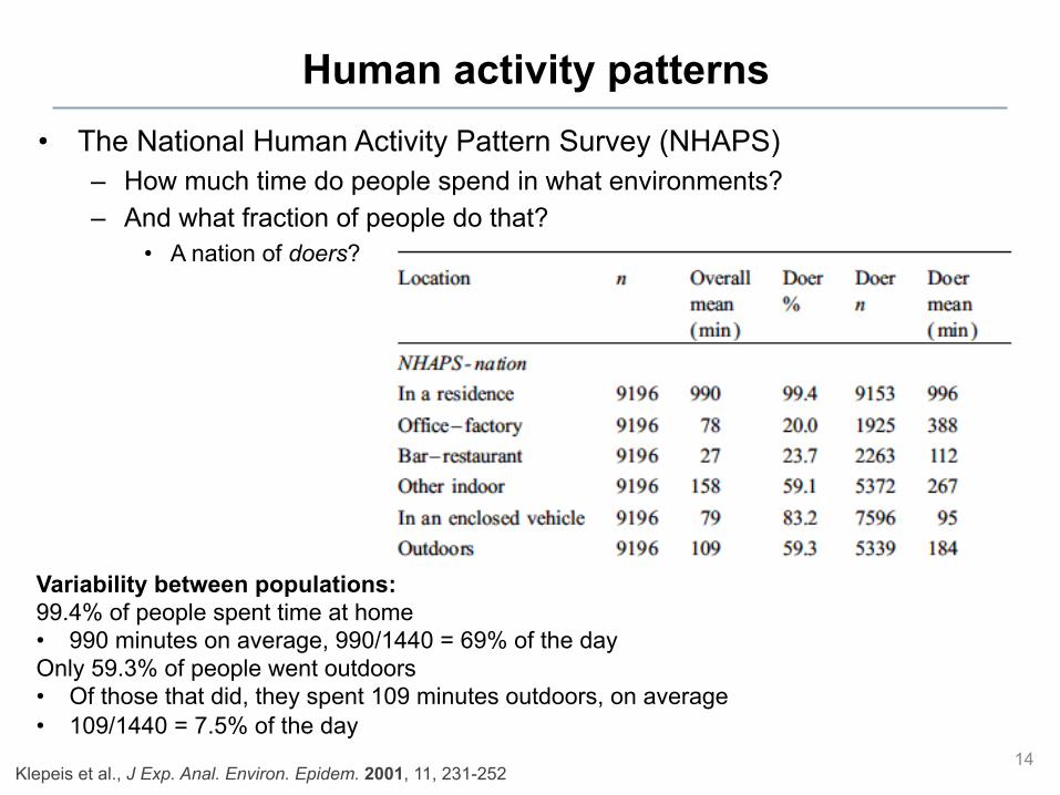
Human activity patterns • The National Human Activity Pattern Survey (NHAPS)
– How much time do people spend in what environments? – And what fraction of people do that?
• A nation of doers?
14 Klepeis et al., J Exp. Anal. Environ. Epidem. 2001, 11, 231-252
Variability between populations: 99.4% of people spent time at home • 990 minutes on average, 990/1440 = 69% of the day Only 59.3% of people went outdoors • Of those that did, they spent 109 minutes outdoors, on average • 109/1440 = 7.5% of the day
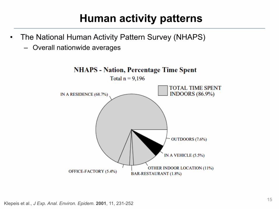
Human activity patterns
15 Klepeis et al., J Exp. Anal. Environ. Epidem. 2001, 11, 231-252
• The National Human Activity Pattern Survey (NHAPS) – Overall nationwide averages
Human activity patterns
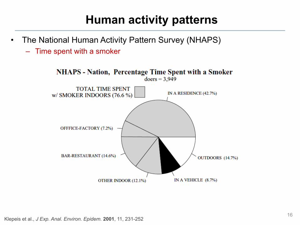
16 Klepeis et al., J Exp. Anal. Environ. Epidem. 2001, 11, 231-252
• The National Human Activity Pattern Survey (NHAPS) – Time spent with a smoker
Human activity patterns
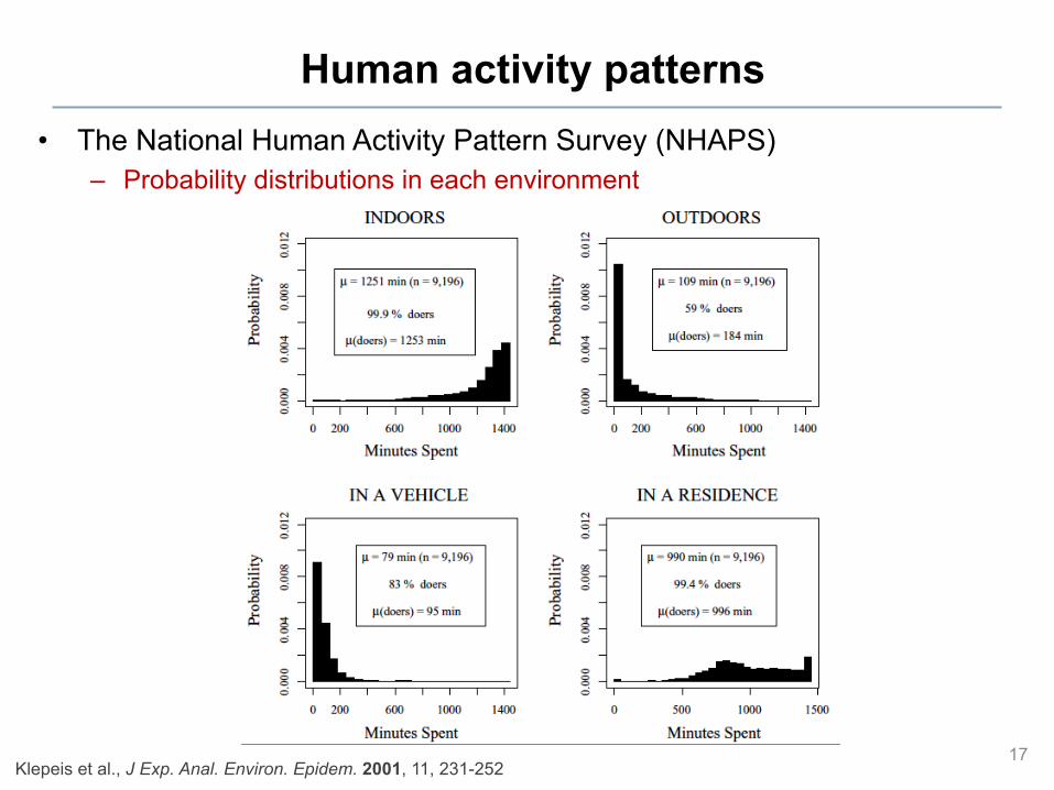
17 Klepeis et al., J Exp. Anal. Environ. Epidem. 2001, 11, 231-252
• The National Human Activity Pattern Survey (NHAPS) – Probability distributions in each environment
Human activity patterns
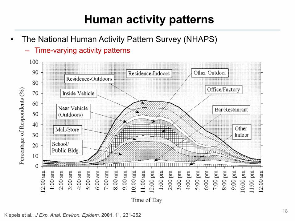
18 Klepeis et al., J Exp. Anal. Environ. Epidem. 2001, 11, 231-252
• The National Human Activity Pattern Survey (NHAPS) – Time-varying activity patterns
Human activity patterns
• What are some other ways to collect human activity data?
19
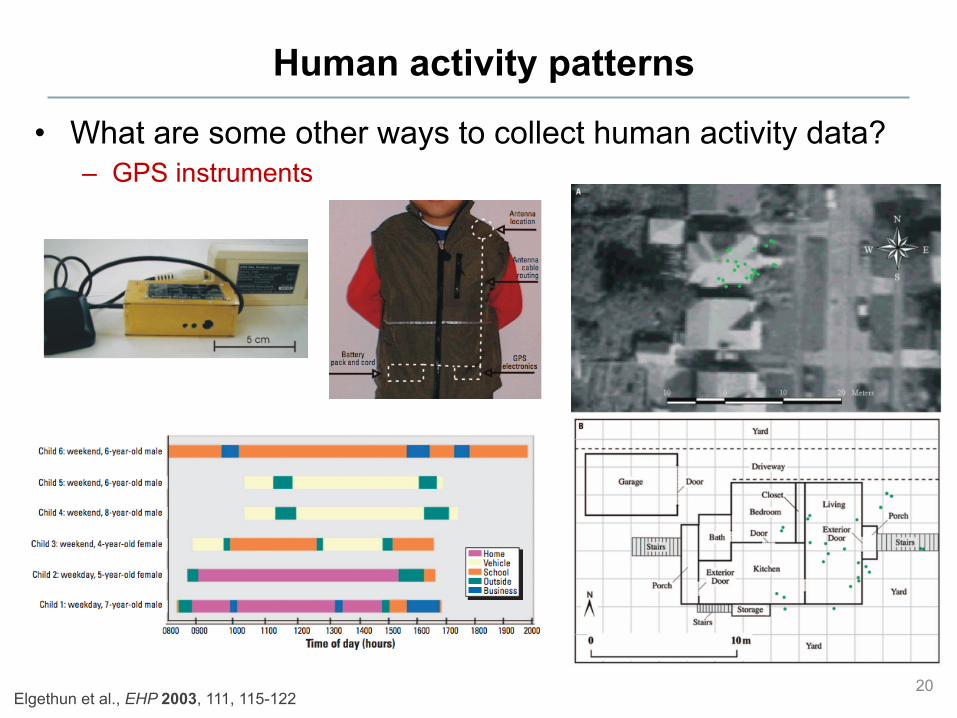
Human activity patterns
• What are some other ways to collect human activity data? – GPS instruments
20 Elgethun et al., EHP 2003, 111, 115-122
Indoor exposures
• So we spend a lot of time indoors (Δtindoor is large) – Do we also encounter large concentrations? (Cindoor)
• Depends on what emissions we’re talking about
• Let’s first discuss “intake fractions”
21
Intake fractions
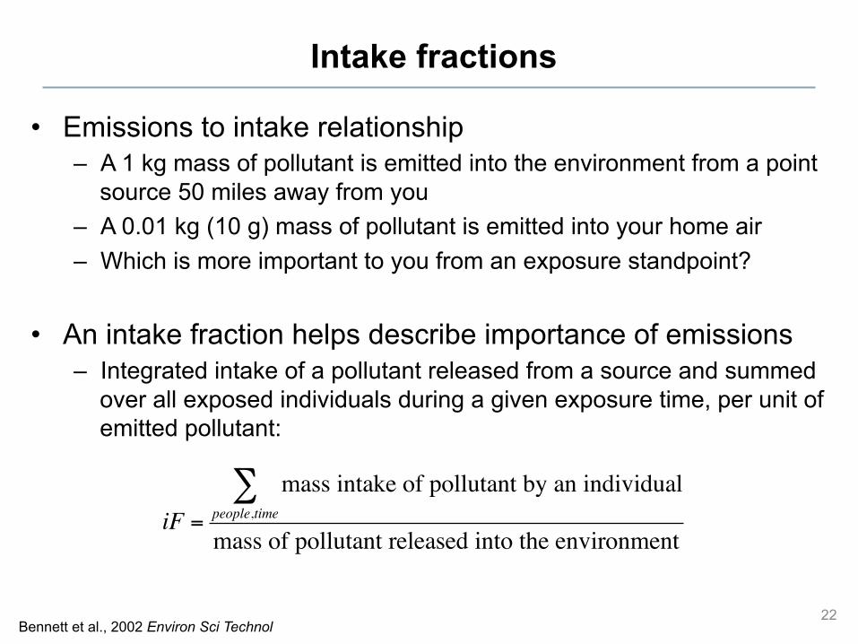
• Emissions to intake relationship – A 1 kg mass of pollutant is emitted into the environment from a point
source 50 miles away from you – A 0.01 kg (10 g) mass of pollutant is emitted into your home air – Which is more important to you from an exposure standpoint?
• An intake fraction helps describe importance of emissions – Integrated intake of a pollutant released from a source and summed
over all exposed individuals during a given exposure time, per unit of emitted pollutant:
22 Bennett et al., 2002 Environ Sci Technol
iF =mass intake of pollutant by an individual
people,time!
mass of pollutant released into the environment
Intake fractions
• Values of iF depend on several factors: – Chemical properties of the contaminant – Emission locations – Environmental conditions – Exposure pathways – Receptor (i.e., human) locations and activities – Population characteristics
23 Bennett et al., 2002 Environ Sci Technol
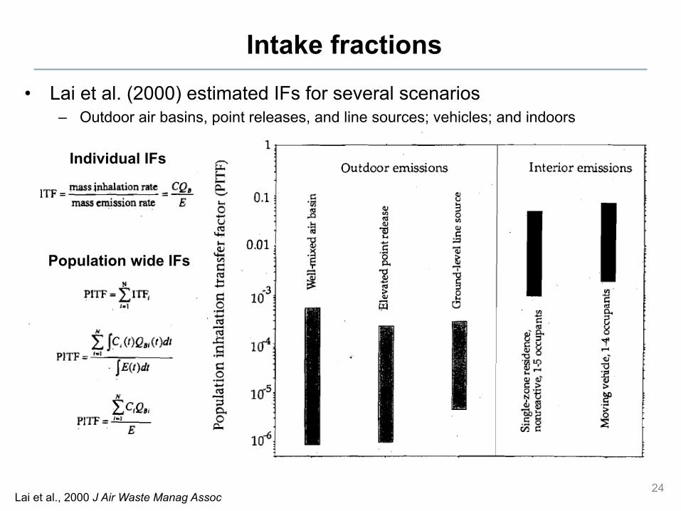
Intake fractions • Lai et al. (2000) estimated IFs for several scenarios
– Outdoor air basins, point releases, and line sources; vehicles; and indoors
24 Lai et al., 2000 J Air Waste Manag Assoc
Individual IFs
Population wide IFs
Intake fraction example
• Benzene example – Benzene is emitted to outdoor air from motor vehicles – Benzene is also present in environmental tobacco smoke (ETS)
• Outdoor benzene in California’s South Cost air basin (SoCAB) – 16,000 km2 area – Home to 14 million people who drive vehicles ~0.5 billion km daily
• They use ~59 million L of gasoline daily • ~280 mg of benzene is emitted per L of gasoline • Total emissions of ~17 metric tons (17000 kg) of benzene per day • Outdoor iFs range approximately 1×10⁻⁶ to 5×10⁻⁴
– Depending on meteorology and other factors
25 Bennett et al., 2002 Environ Sci Technol
Intake fraction example
• Benzene from ETS indoors – SoCAB is also home to ~1.9 million smokers
• Consuming 42 million cigarettes daily – Assume that 50% of cigarettes consumed in the area are smoked in homes – Benzene emission factors for ETS are 280-610 µg per cigarette
• Assume ~450 µg per cigarette – Total estimated residential emissions of benzene from ETS are ~9 kg/day
• That is only ~0.05% of the total emitted by motor vehicles
– But, the iF for a nonreactive pollutant in a residence is ~7×10⁻³ • That is 10-100+ times as high as for outdoor emissions (1×10⁻⁶-5×10⁻⁴)
– Overall, vehicles account for inhalation of ~1 kg/day of benzene inhalation • Across the basin population • ETS accounts for ~60 g/day • So while ETS accounts for only 0.05% of the emissions, it accounts for
~6% of benzene intake in the area – Non-negligible amount (and IF is 120 times higher than E)
26 Bennett et al., 2002 Environ Sci Technol
Intake fractions
• So what was the answer to our original question? – A 1 kg mass of pollutant is emitted into the environment from a point
source 50 miles away from you – A 0.01 kg (10 g) mass of pollutant is emitted into your home air – Which is more important to you from an exposure standpoint?
– Indoor emission is ~1/100th of the outdoor mass emission – But indoor IF is ~10 to ~1000 higher – So the overall effect on intake is generally higher for the indoor
source
27
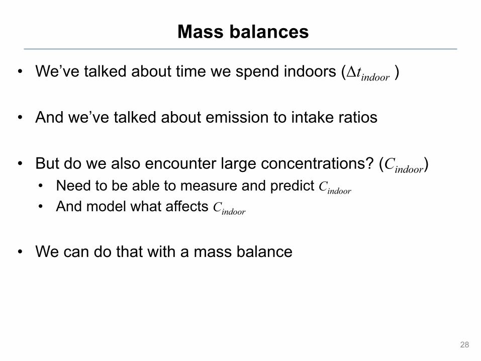
Mass balances
• We’ve talked about time we spend indoors (Δtindoor )
• And we’ve talked about emission to intake ratios
• But do we also encounter large concentrations? (Cindoor) • Need to be able to measure and predict Cindoor • And model what affects Cindoor
• We can do that with a mass balance
28
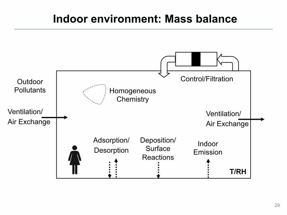
Indoor environment: Mass balance
29
Ventilation/ Air Exchange
Ventilation/ Air Exchange
Outdoor Pollutants
Indoor Emission
Deposition/Surface
Reactions
Adsorption/ Desorption
Homogeneous Chemistry
Control/Filtration
T/RH
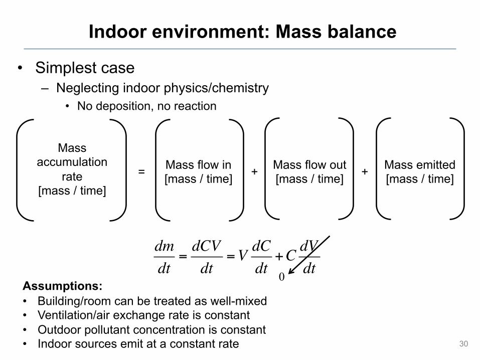
Indoor environment: Mass balance
• Simplest case – Neglecting indoor physics/chemistry
• No deposition, no reaction
30
Mass accumulation
rate [mass / time]
= Mass flow in [mass / time]
Mass flow out [mass / time]
Mass emitted [mass / time] + +
dmdt
=dCVdt
=V dCdt
+C dVdt0
Assumptions: • Building/room can be treated as well-mixed • Ventilation/air exchange rate is constant • Outdoor pollutant concentration is constant • Indoor sources emit at a constant rate
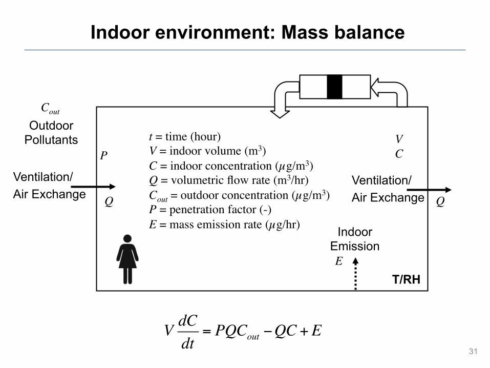
Indoor environment: Mass balance
31
Ventilation/ Air Exchange
Ventilation/ Air Exchange
Outdoor Pollutants
Indoor Emission
T/RH
V dCdt
= PQCout !QC +E
t = time (hour) V = indoor volume (m3) C = indoor concentration (µg/m3) Q = volumetric flow rate (m3/hr) Cout = outdoor concentration (µg/m3) P = penetration factor (-) E = mass emission rate (µg/hr)
Cout
Q
P V
Q
E
C
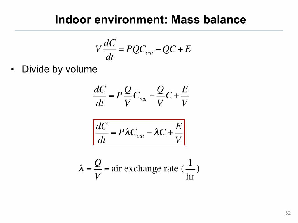
Indoor environment: Mass balance
• Divide by volume
32
V dCdt
= PQCout !QC +E
dCdt
= PQVCout !
QVC + E
V
dCdt
= P!Cout !!C +EV
! =QV= air exchange rate ( 1
hr)
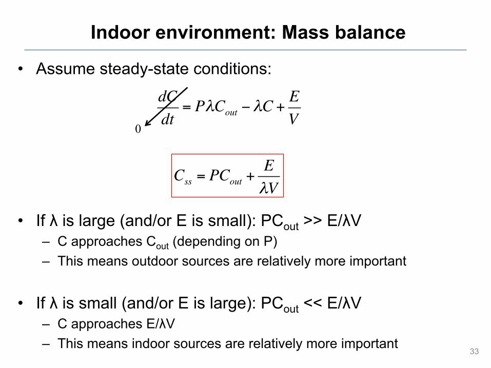
Indoor environment: Mass balance
• Assume steady-state conditions:
• If λ is large (and/or E is small): PCout >> E/λV – C approaches Cout (depending on P) – This means outdoor sources are relatively more important
• If λ is small (and/or E is large): PCout << E/λV – C approaches E/λV – This means indoor sources are relatively more important
33
dCdt
= P!Cout !!C +EV
0
Css = PCout +E!V
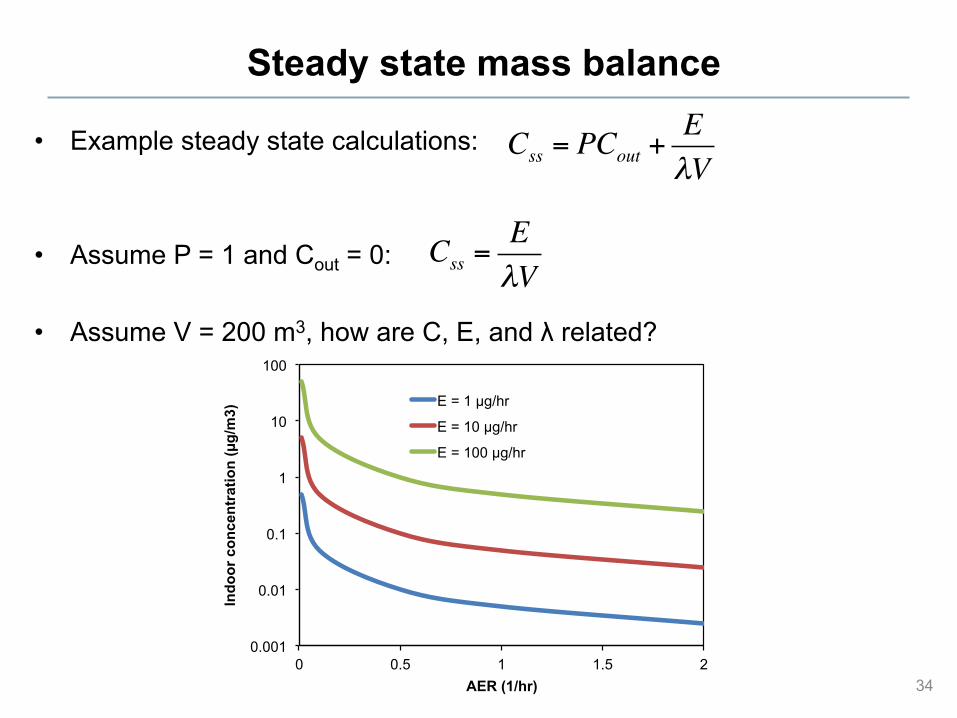
Steady state mass balance
• Example steady state calculations:
• Assume P = 1 and Cout = 0:
• Assume V = 200 m3, how are C, E, and λ related?
34
Css = PCout +E!V
Css =E!V
0.001
0.01
0.1
1
10
100
0 0.5 1 1.5 2
Indo
or c
once
ntra
tion
(!g/
m3)
AER (1/hr)
E = 1 !g/hr
E = 10 !g/hr
E = 100 !g/hr
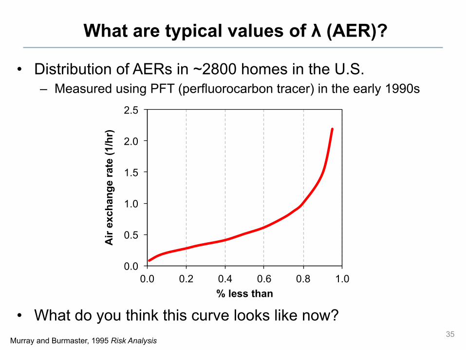
What are typical values of λ (AER)?
• Distribution of AERs in ~2800 homes in the U.S. – Measured using PFT (perfluorocarbon tracer) in the early 1990s
• What do you think this curve looks like now? 35
Murray and Burmaster, 1995 Risk Analysis
0.0
0.5
1.0
1.5
2.0
2.5
0.0 0.2 0.4 0.6 0.8 1.0
Air
exc
hang
e ra
te (1
/hr)
% less than
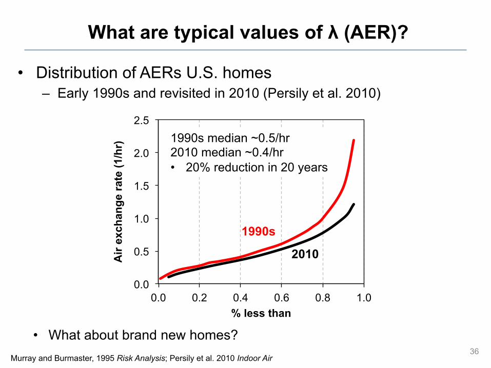
What are typical values of λ (AER)?
• Distribution of AERs U.S. homes – Early 1990s and revisited in 2010 (Persily et al. 2010)
36 Murray and Burmaster, 1995 Risk Analysis; Persily et al. 2010 Indoor Air
0.0
0.5
1.0
1.5
2.0
2.5
0.0 0.2 0.4 0.6 0.8 1.0
Air
exc
hang
e ra
te (1
/hr)
% less than
1990s
2010
• What about brand new homes?
1990s median ~0.5/hr 2010 median ~0.4/hr • 20% reduction in 20 years
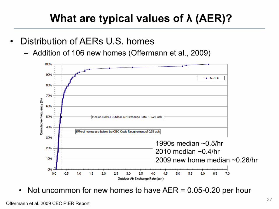
What are typical values of λ (AER)?
• Distribution of AERs U.S. homes – Addition of 106 new homes (Offermann et al., 2009)
37 Offermann et al. 2009 CEC PIER Report
• Not uncommon for new homes to have AER = 0.05-0.20 per hour
1990s median ~0.5/hr 2010 median ~0.4/hr 2009 new home median ~0.26/hr
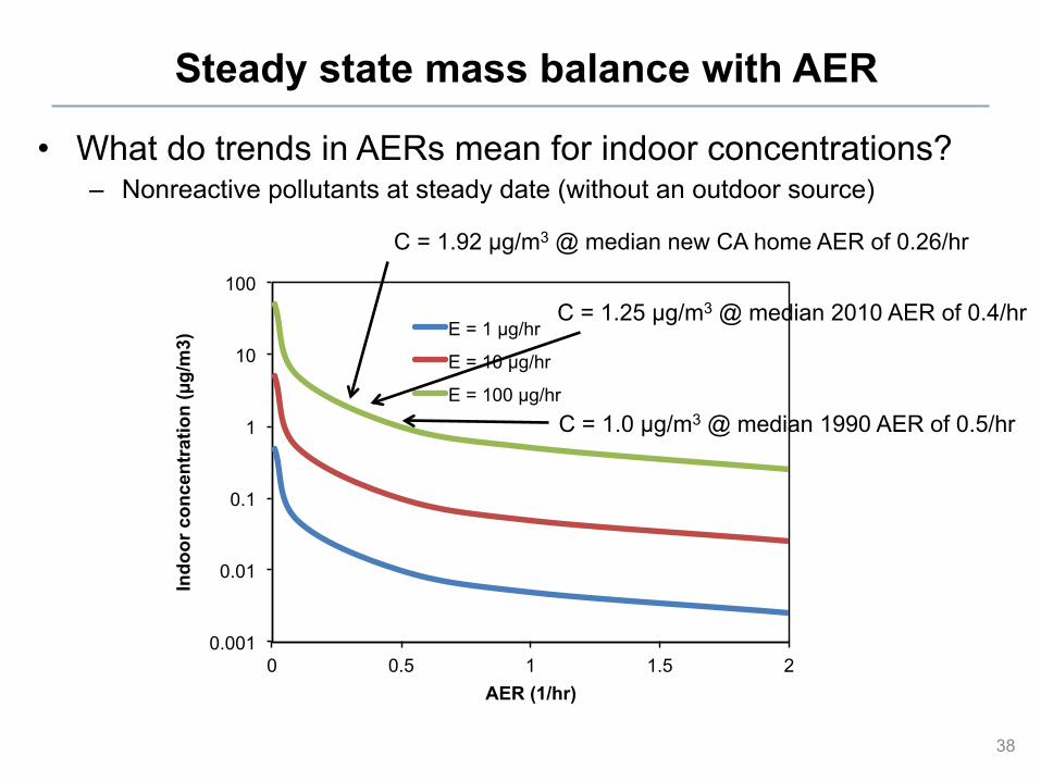
Steady state mass balance with AER
• What do trends in AERs mean for indoor concentrations? – Nonreactive pollutants at steady date (without an outdoor source)
38
0.001
0.01
0.1
1
10
100
0 0.5 1 1.5 2
Indo
or c
once
ntra
tion
(!g/
m3)
AER (1/hr)
E = 1 !g/hr
E = 10 !g/hr
E = 100 !g/hr C = 1.0 µg/m3 @ median 1990 AER of 0.5/hr
C = 1.25 µg/m3 @ median 2010 AER of 0.4/hr
C = 1.92 µg/m3 @ median new CA home AER of 0.26/hr
Limitations to previous mass balance
• Well-mixed assumption – Occupant exposure can be much higher than estimated near source – Cooking, cleaning, vicinity of smoker – Personal cloud or “pig pen” effect is where:
• Assumption of no sinks or transformations – Adsorption, desorption, deposition, and reactions all ignored (for now)
• Assumption of no control of pollutants – No whole building filtration or portable air cleaner (for now)
• Also assumed steady-state – What about dynamic solution?
39
Cpersonal >Cindoor
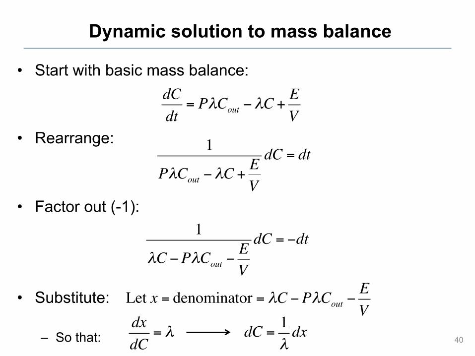
Dynamic solution to mass balance
• Start with basic mass balance:
• Rearrange:
• Factor out (-1):
• Substitute:
– So that: 40
dCdt
= P!Cout !!C +EV
1
P!Cout !!C +EV
dC = dt
1
!C !P!Cout !EV
dC = !dt
Let x = denominator = !C !P!Cout !EV
dxdC
= ! dC = 1!dx
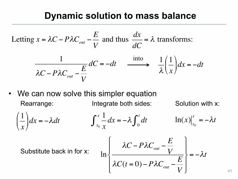
Dynamic solution to mass balance
• We can now solve this simpler equation Rearrange: Integrate both sides: Solution with x: Substitute back in for x:
41
1
!C !P!Cout !EV
dC = !dt
Letting x = !C !P!Cout !EV
and thus dxdC
= ! transforms:
1!1x!
"#$
%&dx = 'dt
into
1x!
"#$
%&dx = '!dt
1xdx
x0
x! = "! dt
0
t! ln(x)
x0
x= !!t
ln!C !P!Cout !
EV
!C(t = 0)!P!Cout !EV
"
#$
%$
&
'$
($= !!t
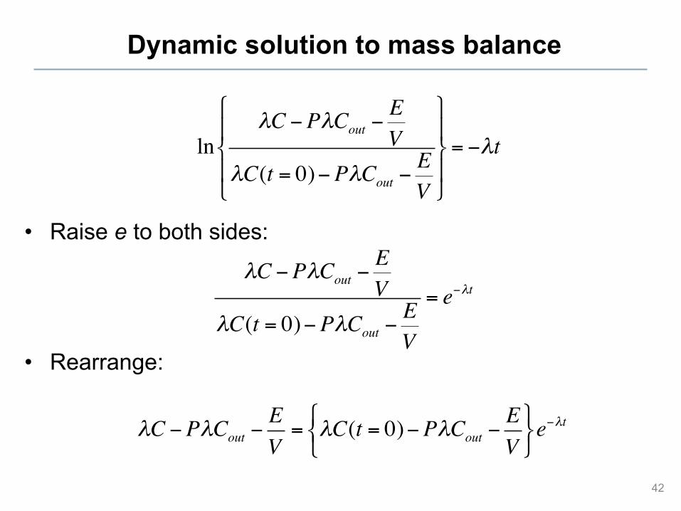
Dynamic solution to mass balance
• Raise e to both sides:
• Rearrange:
42
ln!C !P!Cout !
EV
!C(t = 0)!P!Cout !EV
"
#$
%$
&
'$
($= !!t
!C !P!Cout !EV
!C(t = 0)!P!Cout !EV
= e!!t
!C !P!Cout !EV= !C(t = 0)!P!Cout !
EV
"#$
%&'e!!t
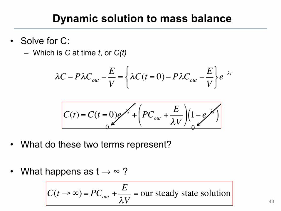
Dynamic solution to mass balance
• Solve for C: – Which is C at time t, or C(t)
• What do these two terms represent?
• What happens as t → ∞ ?
43
!C !P!Cout !EV= !C(t = 0)!P!Cout !
EV
"#$
%&'e!!t
C(t) =C(t = 0)e!!t + PCout +E!V
"
#$
%
&' 1! e!!t( )
C(t!") =PCout +E!V
= our steady state solution
0 0
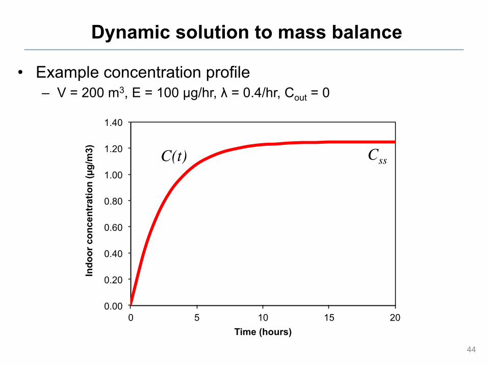
Dynamic solution to mass balance
• Example concentration profile – V = 200 m3, E = 100 µg/hr, λ = 0.4/hr, Cout = 0
44
0.00
0.20
0.40
0.60
0.80
1.00
1.20
1.40
0 5 10 15 20
Indo
or c
once
ntra
tion
(!g/
m3)
Time (hours)
Css C(t)
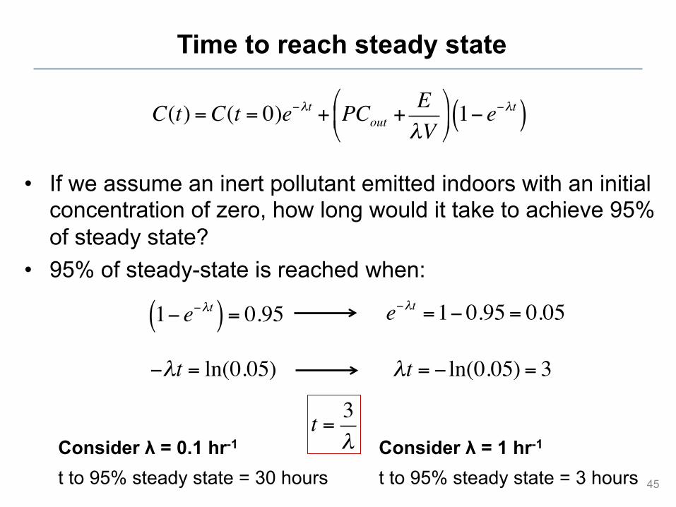
Time to reach steady state
• If we assume an inert pollutant emitted indoors with an initial concentration of zero, how long would it take to achieve 95% of steady state?
• 95% of steady-state is reached when:
45
C(t) =C(t = 0)e!!t + PCout +E!V
"
#$
%
&' 1! e!!t( )
1! e!!t( ) = 0.95 e!!t =1! 0.95= 0.05
!!t = ln(0.05) !t = ! ln(0.05) = 3
t = 3!Consider λ = 0.1 hr-1
t to 95% steady state = 30 hours Consider λ = 1 hr-1
t to 95% steady state = 3 hours
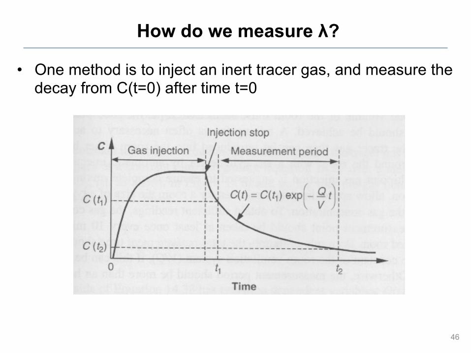
How do we measure λ?
• One method is to inject an inert tracer gas, and measure the decay from C(t=0) after time t=0
46
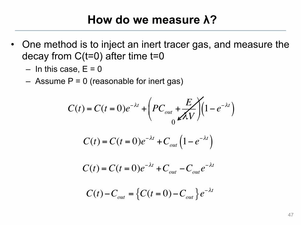
How do we measure λ?
• One method is to inject an inert tracer gas, and measure the decay from C(t=0) after time t=0 – In this case, E = 0 – Assume P = 0 (reasonable for inert gas)
47
C(t) =C(t = 0)e!!t + PCout +E!V
"
#$
%
&' 1! e!!t( )
0
C(t) =C(t = 0)e!!t +Cout 1! e!!t( )
C(t) =C(t = 0)e!!t +Cout !Coute!!t
C(t)!Cout = C(t = 0)!Cout{ }e!!t
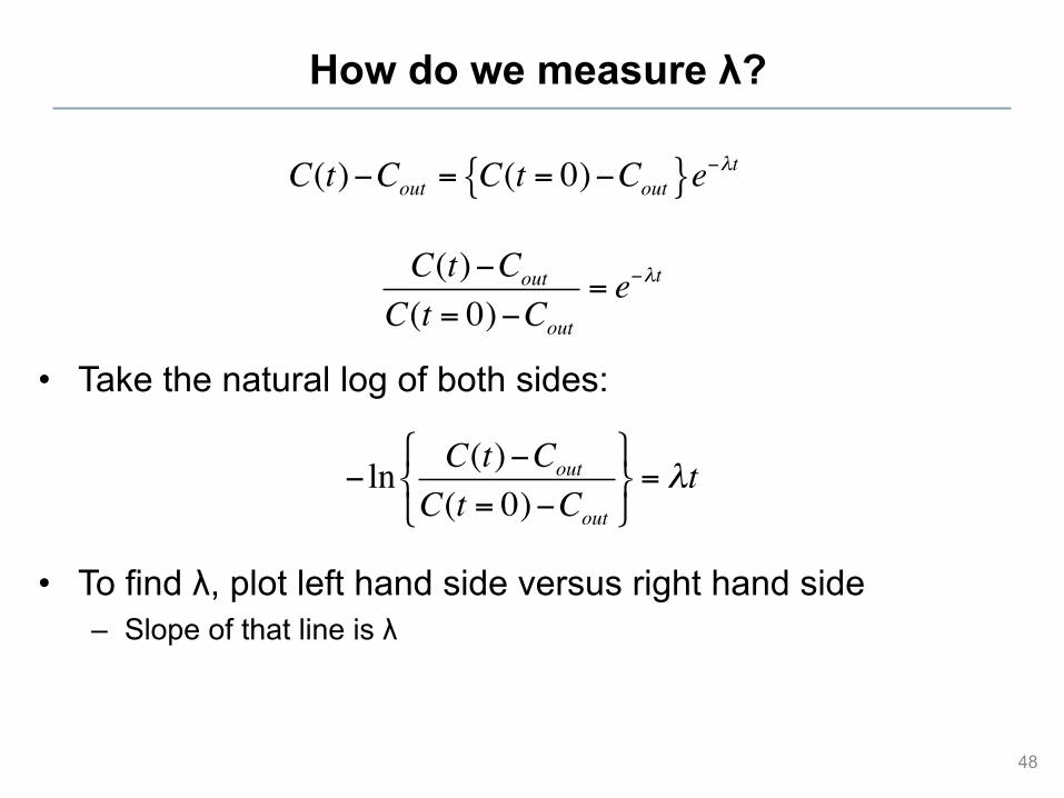
How do we measure λ?
• Take the natural log of both sides:
• To find λ, plot left hand side versus right hand side – Slope of that line is λ
48
C(t)!Cout = C(t = 0)!Cout{ }e!!t
C(t)!Cout
C(t = 0)!Cout
= e!!t
! ln C(t)!Cout
C(t = 0)!Cout
"#$
%&'= !t
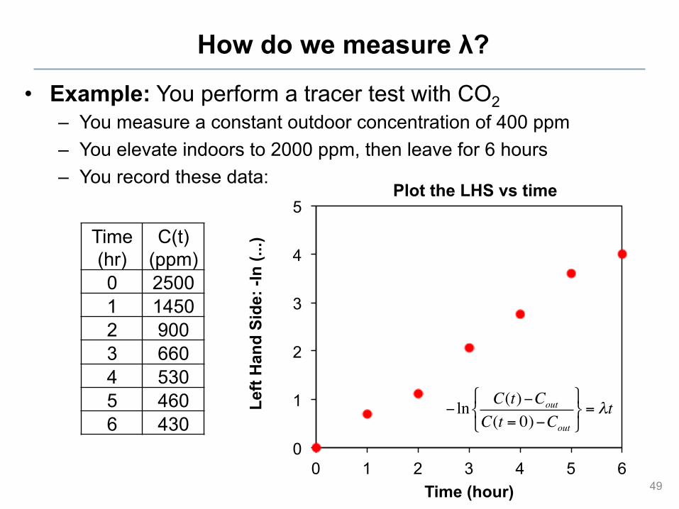
How do we measure λ?
• Example: You perform a tracer test with CO2 – You measure a constant outdoor concentration of 400 ppm – You elevate indoors to 2000 ppm, then leave for 6 hours – You record these data:
0
1
2
3
4
5
0 1 2 3 4 5 6
Left
Han
d Si
de: -
ln (.
..)
Time (hour) 49
Time (hr)
C(t) (ppm)
0 2500 1 1450 2 900 3 660 4 530 5 460 6 430
Plot the LHS vs time
! ln C(t)!Cout
C(t = 0)!Cout
"#$
%&'= !t
y = 0.7058x R! = 0.9997
0
1
2
3
4
5
0 1 2 3 4 5 6
Left
Han
d Si
de: -
ln (.
..)
Time (hour)
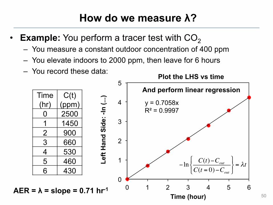
How do we measure λ?
• Example: You perform a tracer test with CO2 – You measure a constant outdoor concentration of 400 ppm – You elevate indoors to 2000 ppm, then leave for 6 hours – You record these data:
50
Time (hr)
C(t) (ppm)
0 2500 1 1450 2 900 3 660 4 530 5 460 6 430
Plot the LHS vs time
And perform linear regression
! ln C(t)!Cout
C(t = 0)!Cout
"#$
%&'= !t
AER = λ = slope = 0.71 hr-1
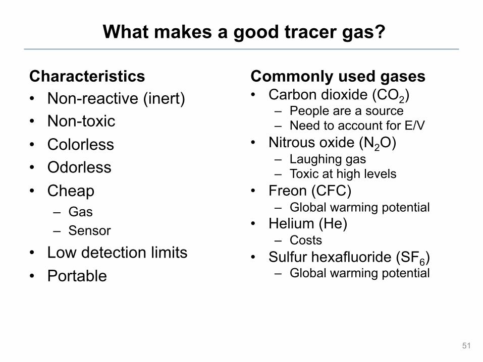
What makes a good tracer gas?
51
• Carbon dioxide (CO2) – People are a source – Need to account for E/V
• Nitrous oxide (N2O) – Laughing gas – Toxic at high levels
• Freon (CFC) – Global warming potential
• Helium (He) – Costs
• Sulfur hexafluoride (SF6) – Global warming potential
• Non-reactive (inert) • Non-toxic • Colorless • Odorless • Cheap
– Gas – Sensor
• Low detection limits • Portable
Characteristics Commonly used gases
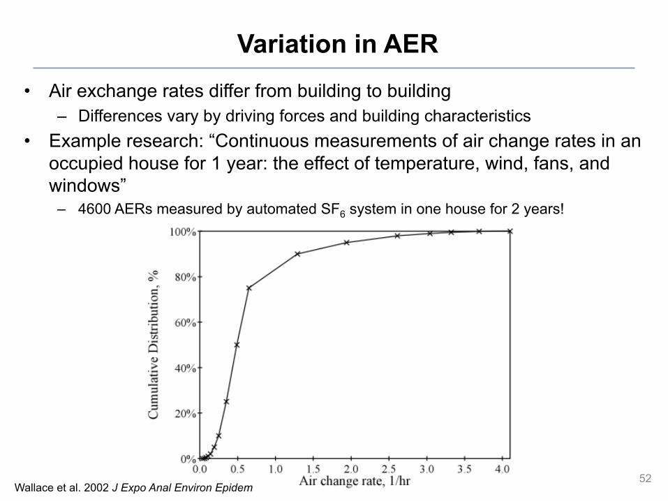
Variation in AER • Air exchange rates differ from building to building
– Differences vary by driving forces and building characteristics • Example research: “Continuous measurements of air change rates in an
occupied house for 1 year: the effect of temperature, wind, fans, and windows”
– 4600 AERs measured by automated SF6 system in one house for 2 years!
52 Wallace et al. 2002 J Expo Anal Environ Epidem
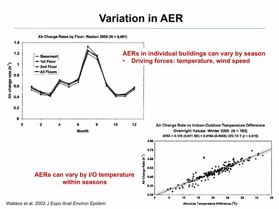
Variation in AER
53 Wallace et al. 2002 J Expo Anal Environ Epidem
AERs in individual buildings can vary by season • Driving forces: temperature, wind speed
AERs can vary by I/O temperature within seasons
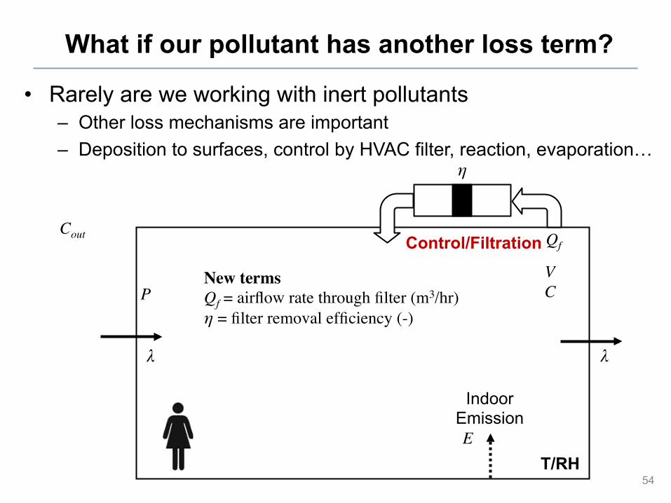
What if our pollutant has another loss term?
• Rarely are we working with inert pollutants – Other loss mechanisms are important – Deposition to surfaces, control by HVAC filter, reaction, evaporation…
54
Indoor Emission
T/RH
Cout
λ
P V
λ
E
C
Control/Filtration
New terms Qf = airflow rate through filter (m3/hr) η = filter removal efficiency (-)
Qf
η
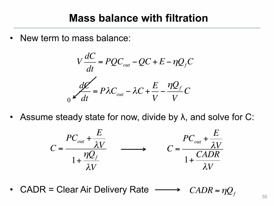
Mass balance with filtration
• New term to mass balance:
• Assume steady state for now, divide by λ, and solve for C:
• CADR = Clear Air Delivery Rate 55
V dCdt
= PQCout !QC +E !!QfC
dCdt
= P!Cout !!C +EV!"Qf
VC
0
C =PCout +
E!V
1+"Qf
!V
C =PCout +
E!V
1+ CADR!V
CADR =!Qf
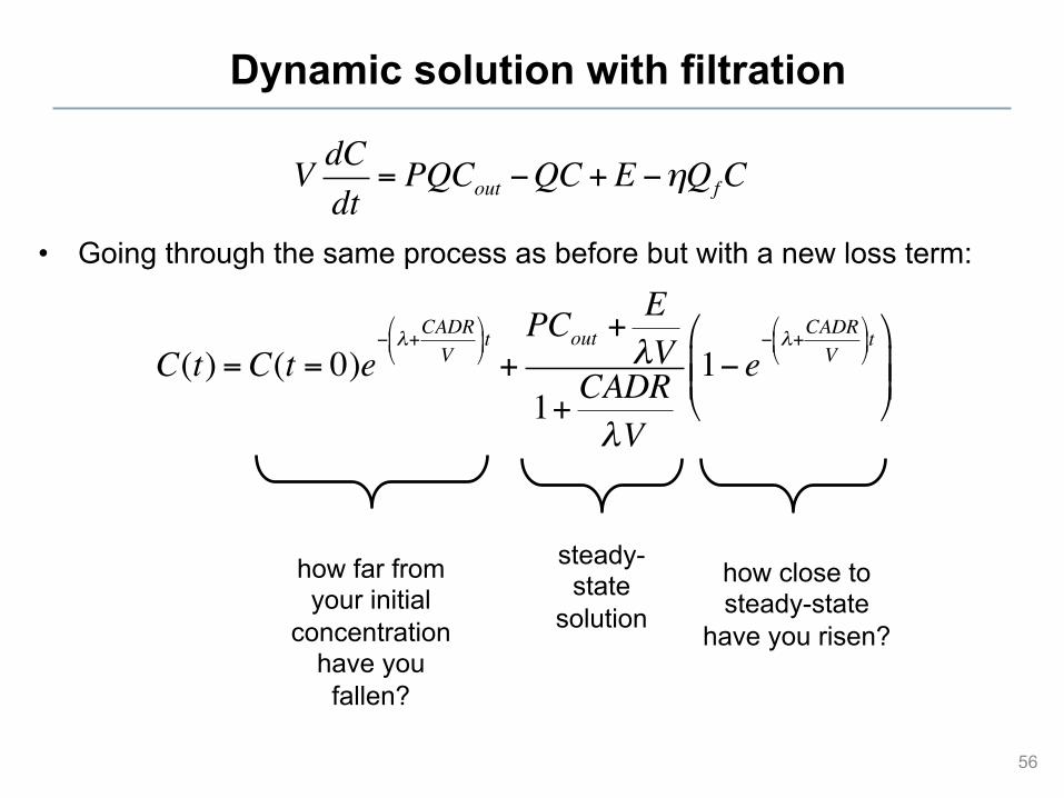
Dynamic solution with filtration
• Going through the same process as before but with a new loss term:
56
V dCdt
= PQCout !QC +E !!QfC
C(t) =C(t = 0)e! !+
CADRV
"
#$
%
&'t+PCout +
E!V
1+ CADR!V
1! e! !+
CADRV
"
#$
%
&'t"
#$$
%
&''
steady-state
solution
how close to steady-state
have you risen?
how far from your initial
concentration have you fallen?
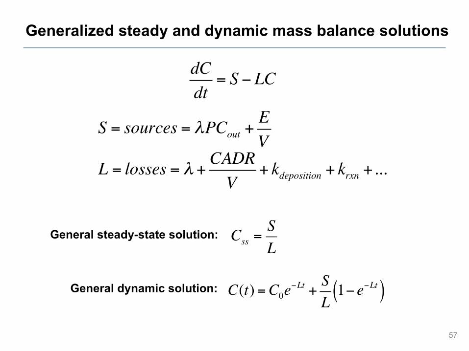
Generalized steady and dynamic mass balance solutions
57
dCdt
= S ! LC
S = sources = !PCout +EV
L = losses = ! + CADRV
+ kdeposition + krxn +...
Css =SL
C(t) =C0e!Lt +
SL1! e!Lt( )
General steady-state solution:
General dynamic solution:
Assignment: HW1
• HW1 has been posted to BB – Covers AER estimation and basic steady state calcs
• Due 1 week from today in class – Upload a PDF, email me a PDF, or turn in hardcopy in class
• I will be at ASHRAE in Dallas Thursday through Tuesday morning – Ask any questions via email
• Tuesday class as scheduled, unless I get delayed in Dallas – In that case, I would email you all Tuesday about postponing
58
Next time
• Overview of indoor pollutants – Particles – Gas-phase compounds – Biological
• Typical concentrations measured in field studies – Will go into individual dynamics later in the course
• Read Weschler paper if interested – How have indoor pollutants changed since the 1950s?
59
Recommended