Energy Markets II:Spread Options, Weather Derivatives & Asset
Valuation
Rene Carmona
Bendheim Center for FinanceDepartment of Operations Research & Financial Engineering
Princeton University
Banff, May 2007
Carmona Energy Markets

The Importance of Spread Options
European Call on the difference between two indexes
Carmona Energy Markets

Calendar Spread Options
Single Commodity at two different times
E{(I(T2)− I(T1)− K )+}
Mathematically easier (only one underlier)
European Call on the difference between two indexes
Calendar SpreadAmaranth largest (and fatal) positions
Shoulder Natural Gas Spread (play on inventories)Long March GasShort April Gas
Depletion stops in March, injection starts in AprilCan be fatal: emphwidow maker spread
Carmona Energy Markets

Seasonality of Gas Inventory
9
There is a long injection season from the spring through the fall when natural gas is
injected and stored in caverns for use during the long winter to meet the higher residential
demand, as in FIGURE 2.1. The figure illustrates the U.S. Department of Energy’s total
(lower 48 states) working underground storage for natural gas inventories over 2006.
Inventories stop being drawn down in March and begin to rise in April. As we will see in
Section 2.1.3.2, the summer and fall futures contracts, when storage is rising, trade at a
discount to the winter contracts, when storage peaks and levels off. Thus, the markets
provide a return for storing natural gas. A storage operator can purchase summer futures
and sell winter futures, the difference being the return for storage. At maturity of the
summer contract, the storage owner can move the delivered physical gas into storage and
release it when the winter contract matures. Storage is worth more if such spread bets are
steep between near and far months.
2.1.3 Risk Management Instruments
Futures and forward contracts, swaps, spreads and options are the most standard
tools for speculation and risk management in the natural gas market. Commodities market
U.S. Natural Gas Inventories 2005-6
1,500
2,000
2,500
3,000
3,500
12/24/05
2/12/06
4/3/065/23/06
7/12/06
8/31/06
10/20/06
12/9/06
Wee
kly
Stor
age
in B
illio
n C
ubic
Fee
t
FIGURE 2.1: Seasonality in Natural Gas Weekly Storage (from Raj Hatharamani ORFE Senior Thesis)
Carmona Energy Markets

What Killed Amaranth 43
November 2006 bets were particularly large compared to the rest, as Amaranth accumulated
the largest ever long position in the November futures contract in the month preceding its
downfall. Regarding the Fund’s overall strategy, Burton and Strasburg (2006a) write that
Amaranth was generally long winter contracts and short summer and fall ones, a winning bet
since 2004. Other sources affirm that Amaranth was long the far-end of the curve and short
the front-end, and their positions lost value when far-forward gas contracts fell more than
near-term contracts did in September 2006.
From these bets, Amaranth believed a stormy and exceptionally cold winter in 2006
would result in excess usage of natural gas in the winter and a shortage in March of the
following year. Higher demand would result in a possible stockout by the end of February
and higher March prices. Yet April prices would fall as supply increases at the start of the
injection season. In this scenario, there is theoretically no ceiling on how much the price of
the March contract can rise relative to the rest of the curve. Fischer (2006), natural gas
trader at Chicago-based hedge fund Citadel Investment Group, believes Amaranth bet on
similar hurricane patterns in the previous two years. As a result, the extreme event that hurt
Amaranth was that nothing happened—there was no Hurricane Katrina or similar
Shoulder Month Spread
0
0.5
1
1.5
2
2.5
3
Dec-04 Apr-05 Jul-05 Oct-05 Feb-06 May-06 Aug-06 Nov-06
$ pe
r m
m B
tu
2007 2008 2009 2010 2011
FIGURE 3.1: Natural Gas March-April Contract Spread Evolution (from Raj Hatharamani ORFE Senior Thesis)
Carmona Energy Markets

More Spread Options
Cross CommodityCrush Spread: between Soybean and soybean products (meal &oil)Crack Spread:
gasoline crack spread between Crude and Unleadedheating oil crack spread between Crude and HO
Spark spreadSt = FE(t)− Heff FG(t)
Heff Heat Rate
Carmona Energy Markets

Synthetic Generation
Present value of profits for future power generation (case of one fuel)
E{∫ T
0D(0, t)(FP(t , τ)− H ∗ FG(t , τ)− K )+ dt
}where
τ > 0 fixed (small)D(0, t) discount factor to compute present values
FP(t , τ) (resp. FG(t , τ)) price at time t of a power (resp. gas)contract with delivery t + τ
H Heat RateK Operation and Maintenance cost (sometimes denoted O&M)
Carmona Energy Markets
Basket of Spread OptionsDeterministic discounting (with constant interest rate)
D(t ,T ) = e−r(T−t)
Interchange expectation and integral∫ T
0e−rtE{(FP(t , τ)− H ∗ FG(t , τ)− K )+} dt
Continuous stream of spread optionsIn Practice
Discretize time, say daily
T∑t=0
e−rtE{(FP(t , τ)− H ∗ FG(t , τ)− K )+
Bin Daily Production in Buckets Bk ’s (e.g. 5× 16, 2× 16, 7× 8,settlement locations, .....).
T∑t=0
e−r(T−t)∑
k
E{(F (k)P (t , τ)− H(k) ∗ F (k)
G (t , τ)− K (k))+}
Basket of Spark Spread Options
Carmona Energy Markets
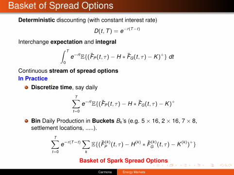
Spread Mathematical Challenge
p = e−rT E{(I2(T )− I1(T )− K )+}
Underlying indexes are spot pricesGeometric Brownian Motions (K = 0 Margrabe)Geometric Ornstein-Uhlembeck (OK for Gas)Geometric Ornstein-Uhlembeck with jumps (OK for Power)
Underlying indexes are forward/futures pricesHJM-type models with deterministic coefficients
Problem
finding closed form formula and/or fast/sharp approximation for
E{(αeγX1 − βeδX2 − κ)+}
for a Gaussian vector (X1,X2) of N(0, 1) random variables with correlation ρ.
Sensitivities?
Carmona Energy Markets

Easy Case : Exchange Option & Margrabe Formula
p = e−rT E{(S2(T )− S1(T ))+}
S1(T ) and S2(T ) log-normalp given by a formula a la Black-Scholes
p = x2Φ(d1)− x1Φ(d0)
with
d1 =ln(x2/x1)
σ√
T+
12σ√
T d0 =ln(x2/x1)
σ√
T− 1
2σ√
T
and:
x1 = S1(0), x2 = S2(0), σ2 = σ21 − 2ρσ1σ2 + σ2
2
Deltas are also given by ”closed form formulae”.
Carmona Energy Markets

Proof of Margrabe Formula
p = e−rT EQ{(S2(T )− S1(T )
)+} = e−rT EQ
{(S2(T )
S1(T )− 1)+
S1(T )
}
Q risk-neutral probability measure
Define ( Girsanov) P by:
dPdQ
∣∣∣∣FT
= S1(T ) = exp(−1
2σ2
1T + σ1W1(T )
)Under P,
W1(t)− σ1t and W2(t)S2/S1 is geometric Brownian motion under P with volatility
σ2 = σ21 − 2ρσ1σ2 + σ2
2
p = S1(0)EP
{(S2(T )
S1(T )− 1)+}
Black-Scholes formula with K = 1, σ as above.
Carmona Energy Markets

(Classical) Real Option Power Plant Valuation
Real Option ApproachLifetime of the plant [T1,T2]
C capacity of the plant (in MWh)
H heat rate of the plant (in MMBtu/MWh)
Pt price of power on day t
Gt price of fuel (gas) on day t
K fixed Operating Costs
Value of the Plant (ORACLE)
CT2∑
t=T1
e−rtE{(Pt − HGt − K )+}
String of Spark Spread Options
Carmona Energy Markets

Beyond Plant Valuation: Credit Enhancement
(Flash Back)The Calpine - Morgan Stanley Deal
Calpine needs to refinance USD 8 MM by November 2004Jan. 2004: Deutsche Bank: no traction on the offeringFeb. 2004: The Street thinks Calpine is ”heading South”March 2004: Morgan Stanley offers a (complex) structured deal
A strip of spark spread options on 14 Calpine plantsA similar bond offering
How were the options priced?By Morgan Stanley ?By Calpine ?
Carmona Energy Markets

Calpine Debt
Carmona Energy Markets
Calpine Debt with Deutsche Bank Financing
Carmona Energy Markets

Calpine Debt with Morgan Stanley Financing
Carmona Energy Markets

A Possible ModelAssume that Calpine owns only one plant
MS guarantees its spark spread will be at least κ for M years
Approach a la Leland’s Theory of the Value of the Firm
V = v − p0 + supτ≤T
E{∫ τ
0e−rtδt dt
}where
δt =
{(Pt − H ∗Gt − K ) ∨ κ− ct if 0 ≤ t ≤ M(Pt − H ∗Gt − K )+ − ct if M ≤ t ≤ T
andv current value of firm’s assets
p0 option premium
M length of the option life
κ strike of the option
ct cost of servicing the existing debt
Carmona Energy Markets

Default Time
Carmona Energy Markets

Plant Value
Carmona Energy Markets

Debt Value
Carmona Energy Markets

Pricing Calendar Spreads in Forward Models
Involves prices of two forward contracts with different maturities, sayT1 and T2
S1(t) = F (t ,T1) and S2(t) = F (t ,T2),
Remember forward prices are log-normal
Price at time t of a calendar spread option with maturity T and strikeK
α = e−r [T−t]F (t ,T2), β =
√√√√ n∑k=1
∫ T
tσk (s,T2)2ds,
γ = e−r [T−t]F (t ,T1), and δ =
√√√√ n∑k=1
∫ T
tσk (s,T1)2ds
and κ = e−r(T−t) (µ ≡ 0 per risk-neutral dynamics)
ρ =1βδ
n∑k=1
∫ T
tσk (s,T1)σk (s,T2) ds
Carmona Energy Markets
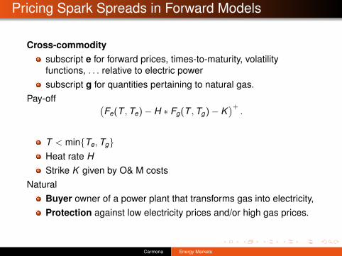
Pricing Spark Spreads in Forward Models
Cross-commoditysubscript e for forward prices, times-to-maturity, volatilityfunctions, . . . relative to electric powersubscript g for quantities pertaining to natural gas.
Pay-off (Fe(T ,Te)− H ∗ Fg(T ,Tg)− K
)+.
T < min{Te,Tg}Heat rate HStrike K given by O& M costs
NaturalBuyer owner of a power plant that transforms gas into electricity,Protection against low electricity prices and/or high gas prices.
Carmona Energy Markets
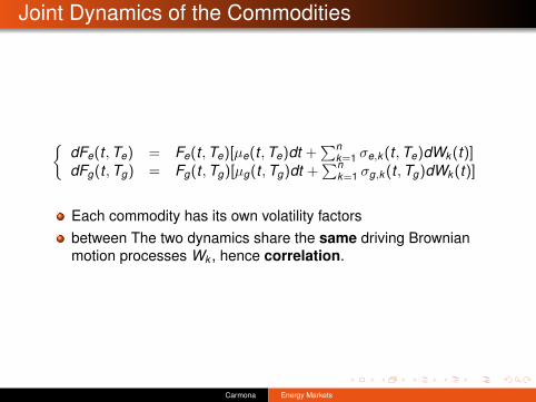
Joint Dynamics of the Commodities
{dFe(t ,Te) = Fe(t ,Te)[µe(t ,Te)dt +
∑nk=1 σe,k (t ,Te)dWk (t)]
dFg(t ,Tg) = Fg(t ,Tg)[µg(t ,Tg)dt +∑n
k=1 σg,k (t ,Tg)dWk (t)]
Each commodity has its own volatility factorsbetween The two dynamics share the same driving Brownianmotion processes Wk , hence correlation.
Carmona Energy Markets

Fitting Join Cross-Commodity Models
on any given day t we haveelectricity forward contract prices for N(e) times-to-maturityτ
(e)1 < τ
(e)2 , . . . < τ
(e)
N(e)
natural gas forward contract prices for N(g) times-to-maturityτ
(g)1 < τ
(g)2 , . . . < τ
(g)
N(g)
Typically N(e) = 12 and N(g) = 36 (possibly more).Estimate instantaneous vols σ(e)(t) & σ(g)(t) 30 days rolling windowFor each day t , the N = N(e) + N(g) dimensional random vector X(t)
X(t) =
(
log Fe(t+1,τ(e)j )−log Fe(t,τ (e)
j )
σ(e)(t)
)j=1,...,N(e)(
log Fg (t+1,τ(g)j )−log Fg (t,τ (g)
j )
σ(g)(t)
)j=1,...,N(g)
Run PCA on historical samples of X(t)Choose small number n of factorsfor k = 1, . . . , n,
first N(e) coordinates give the electricity volatilities τ ↪→ σ(e)k (τ) for
k = 1, . . . , nremaining N(g) coordinates give the gas volatilities τ ↪→ σ
(g)k (τ).
Skip gory detailsCarmona Energy Markets

Pricing a Spark Spread Option
Price at time t
pt = e−r(T−t)Et{(Fe(T ,Te)− H ∗ Fg(T ,Tg)− K )+
}Fe(T ,Te) and Fg(T ,Tg) are log-normal under the pricing measure calibratedby PCA
Fe(T ,Te) = Fe(t ,Te) exp
[−1
2
n∑k=1
∫ T
tσe,k (s,Te)
2ds +n∑
k=1
∫ T
tσe,k (s,Te)dWk (s)
]
and:
Fg(T ,Tg) = Fg(t ,Tg) exp
[−1
2
n∑k=1
∫ T
tσg,k (s,Tg)
2ds +n∑
k=1
∫ T
tσg,k (s,Tg)dWk (s)
]
SetS1(t) = H ∗ Fg(t ,Tg) and S2(t) = Fe(t ,Te)
Carmona Energy Markets
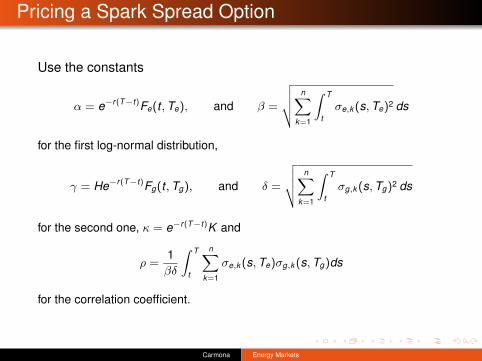
Pricing a Spark Spread Option
Use the constants
α = e−r(T−t)Fe(t ,Te), and β =
√√√√ n∑k=1
∫ T
tσe,k (s,Te)2 ds
for the first log-normal distribution,
γ = He−r(T−t)Fg(t ,Tg), and δ =
√√√√ n∑k=1
∫ T
tσg,k (s,Tg)2 ds
for the second one, κ = e−r(T−t)K and
ρ =1βδ
∫ T
t
n∑k=1
σe,k (s,Te)σg,k (s,Tg)ds
for the correlation coefficient.
Carmona Energy Markets

Approximations
Fourier Approximations (Madan, Carr, Dempster, . . .)Bachelier approximationZero-strike approximationKirk approximationUpper and Lower Bounds
Can we also approximate the Greeks ?
Carmona Energy Markets

Bachelier Approximation
Generate x (1)1 , x (1)
2 , · · · , x (1)N from N(µ1, σ
21)
Generate x (2)1 , x (2)
2 , · · · , x (2)N from N(µ1, σ
21)
Correlation ρLook at the distribution of
ex (2)1 − ex (1)
1 ,ex (2)2 − ex (1)
2 , · · · ,ex (2)N − ex (1)
N
Carmona Energy Markets

Log-Normal Samples
Carmona Energy Markets

Carmona Energy Markets

Bachelier Approximation
Assume (S2(T )− S1(T ) is GaussianMatch the first two moments
p =(
m(T )− Ke−rT)
Φ
(m(T )− Ke−rT
s(T )
)+ s(T )ϕ
(m(T )− Ke−rT
s(T )
)
with:
m(T ) = (x2 − x1)e(µ−r)T
s2(T ) = e2(µ−r)T[x2
1
(eσ2
1T − 1)− 2x1x2
(eρσ1σ2T − 1
)+ x2
2
(eσ2
2T − 1)]
Easy to compute the Greeks !
Carmona Energy Markets

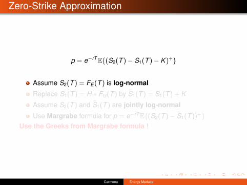
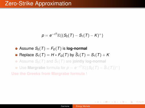
Zero-Strike Approximation
p = e−rT E{(S2(T )− S1(T )− K )+}
Assume S2(T ) = FE(T ) is log-normal
Replace S1(T ) = H ∗ FG(T ) by S1(T ) = S1(T ) + K
Assume S2(T ) and S1(T ) are jointly log-normal
Use Margrabe formula for p = e−rT E{(S2(T )− S1(T ))+}Use the Greeks from Margrabe formula !
Carmona Energy Markets
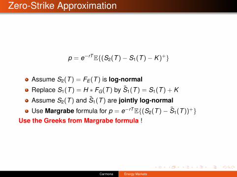

Kirk Approximation
pK = x2Φ
ln(
x2x1+Ke−rT
)σK +
σK
2
−(x1+Ke−rT )Φ
ln(
x2x1+Ke−rT
)σK − σK
2
where
σK =
√σ2
2 − 2ρσ1σ2x1
x1 + Ke−rT + σ21
(x1
x1 + Ke−rT
)2
.
Exactly what we called ”Zero Strike Approximation”!!!
Carmona Energy Markets

Upper and Lower Bounds
Π(α, β, γ, δ, κ, ρ) = E{(
αeβX1−β2/2 − γeδX2−δ2/2 − κ)+}
whereα, β, γ, δ and κ real constantsX1 and X2 are jointly Gaussian N(0,1)
correlation ρα = x2e−q2T β = σ2
√T γ = x1e−q1T δ = σ1
√T and κ = Ke−rT .
Carmona Energy Markets

A Precise Lower Bound
p = x2e−q2T Φ(
d∗ + σ2 cos(θ∗ + φ)√
T)− x1e−q1T Φ
(d∗ + σ1 sin θ∗
√T)
− Ke−rT Φ(d∗)
whereθ∗ is the solution of
1δ cos θ
ln(− βκ sin(θ + φ)
γ[β sin(θ + φ)− δ sin θ]
)− δ cos θ
2
=1
β cos(θ + φ)ln(− δκ sin θα[β sin(θ + φ)− δ sin θ]
)− β cos(θ + φ)
2
the angle φ is defined by setting ρ = cosφd∗ is defined by
d∗ =1
σ cos(θ∗ − ψ)√
Tln(
x2e−q2Tσ2 sin(θ∗ + φ)
x1e−q1Tσ1 sin θ∗
)−1
2(σ2 cos(θ∗+φ)+σ1 cos θ∗)
√T
the angles φ and ψ are chosen in [0, π] such that:
cosφ = ρ and cosψ =σ1 − ρσ2
σ,
Carmona Energy Markets

Remarks on this Lower Bound
p is equal to the true price p whenK = 0x1 = 0x2 = 0ρ = −1ρ = +1
Margrabe formula when K = 0 because
θ∗ = π + ψ = π + arccos(σ1 − ρσ2
σ
).
with:σ =
√σ2
1 − 2ρσ1σ2 + σ22
Carmona Energy Markets

Remarks on this Lower Bound
p is equal to the true price p whenK = 0x1 = 0x2 = 0ρ = −1ρ = +1
Margrabe formula when K = 0 because
θ∗ = π + ψ = π + arccos(σ1 − ρσ2
σ
).
with:σ =
√σ2
1 − 2ρσ1σ2 + σ22
Carmona Energy Markets

Delta Hedging
The portfolio comprising at each time t ≤ T
∆1 = −e−q1T Φ(
d∗ + σ1 cos θ∗√
T)
and∆2 = e−q2T Φ
(d∗ + σ2 cos(θ∗ + φ)
√T)
units of each of the underlying assets is a sub-hedge
its value at maturity is a.s. a lower bound for the pay-off
Carmona Energy Markets

The Other Greeks
� ϑ1 and ϑ2 sensitivities w.r.t. volatilities σ1 and σ2� χ sensitivity w.r.t. correlation ρ� κ sensitivity w.r.t. strike price K� Θ sensitivity w.r.t. maturity time T
ϑ1 = x1e−q1Tϕ(
d∗ + σ1 cos θ∗√
T)
cos θ∗√
T
ϑ2 = −x2e−q2Tϕ(
d∗ + σ2 cos(θ∗ + φ)√
T)
cos(θ∗ + φ)√
T
χ = −x1e−q1Tϕ(
d∗ + σ1 cos θ∗√
T)σ1
sin θ∗
sinφ
√T
κ = −Φ (d∗) e−rT
Θ =σ1ϑ1 + σ2ϑ2
2T− q1x1∆1 − q2x2∆2 − rKκ
Carmona Energy Markets

Comparisons
Behavior of the tracking error as the number of re-hedging times increases.The model data are x1 = 100, x2 = 110, σ1 = 10%, σ2 = 15% and T = 1.ρ = 0.9, K = 30 (left) and ρ = 0.6, K = 20 (right).
Carmona Energy Markets

Generalization: European Basket Option
Black-Scholes Set-UpMultidimensional modeln stocks S1, . . . ,Sn
Risk neutral dynamics
dSi(t)Si(t)
= rdt +n∑
j=1
σijdBj(t),
initial values S1(0), . . . ,Sn(0)B1, . . . ,Bn independent standard Brownian motionsCorrelation through matrix (σij)
Carmona Energy Markets

European Basket Option (cont.)
Vector of weights (wi)i=1,...,n (most often wi ≥ 0)Basket option struck at K at maturity T given by payoff(
n∑i=1
wiSi(T )− K
)+
(Asian Options)
Risk neutral valuation: price at time 0
p = e−rT E
(
n∑i=1
wiSi(T )− K
)+
Carmona Energy Markets

Existing Literature
Jarrow and RuddReplace true distribution by simpler distribution with same firstmomentsEdgeworth (Charlier) expansionsBachelier approximation when Gaussian distribution used
SemiParametric Bounds (known marginals)Fully NonParametric Bounds
Intervals too largeUsed only to rule out arbitrage
Replacing Arithmetic Averages by Geometric Averages (Musiela)
Carmona Energy Markets

Reformulation of the Problem
Change wi if necessary to absorb exponent meanChange wi if necessary to introduce variance in exponentReplace K by −w0eG0−var{G0}/2 with G0 ∼ N(0,0)
Set xi = |wi | and εi = sign(wi)
Our original problem becomes: Compute
E{X+}
for
X =n∑
i=0
εixieGi−Var(Gi )/2.
Carmona Energy Markets

What Are We Looking For?
Explicit formulae in close formCompute Greeks as well
n = 1Black Scholes FormulaMargrabe Formula
Carmona Energy Markets

Two Optimization Problems
For any X ∈ L1,
sup0≤Y≤1
E{XY} = E{X+} = infX=Z1−Z2,Z1≥0,Z2≥0
E{Z1}.
Carmona Energy Markets

Lower Bound Strategy
sup0≤Y≤1
E{XY} = E{X+}
Compute sup in LHS restricting YWe choose Y = 1{u·G≤d} for u ∈ Rn+1 and d ∈ R
where G = (G0,G1, . . . ,Gn) and u ·G = u0G0 + u1G1 + . . .+ unGn
Can we compute?
p∗ = supu,d
E{
X1{u·G≤d}}
We sure can!
E{
X1{u·G≤d}}
=n∑
i=0
E{εixiE{eGi−Var(Gi )/2|u ·G}1{u·G≤d}
}
Carmona Energy Markets

Lower Bound
p∗ = supd∈R
supu·Σu=1
n∑i=0
εixiΦ (d + (Σu)i)
= supd∈R
sup‖v‖=1
n∑i=0
εixiΦ(
d + σi(√
Cv)i
).
whereC = DΣD and D = diag(1/σi)
and
ϕ(x) =1√2π
e−x2/2 and Φ(x) =1√2π
∫ x
−∞e−u2/2du.
Carmona Energy Markets

First Order ConditionsLagrangian L:
L(v ,d) =n∑
i=0
εixiΦ(
d + σi(√
Cv)i
)− µ
2(‖v‖2 − 1
).
p∗ =n∑
i=0
εixiΦ(
d∗ + σi(√
Cv∗)i
)
where d∗ and v∗ satisfy the following first order conditionsn∑
i=0
εixiσi
√C ijϕ
(d∗ + σi(
√Cv∗)i
)− µv∗j = 0 for j = 0, . . . , n
n∑i=0
εixiϕ(
d∗ + σi(√
Cv∗)i
)= 0
‖v∗‖ = 1.
Carmona Energy Markets
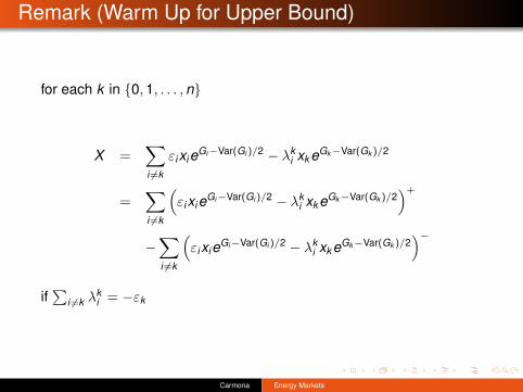
Remark (Warm Up for Upper Bound)
for each k in {0,1, . . . ,n}
X =∑i 6=k
εixieGi−Var(Gi )/2 − λki xk eGk−Var(Gk )/2
=∑i 6=k
(εixieGi−Var(Gi )/2 − λk
i xk eGk−Var(Gk )/2)+
−∑i 6=k
(εixieGi−Var(Gi )/2 − λk
i xk eGk−Var(Gk )/2)−
if∑
i 6=k λki = −εk
Carmona Energy Markets

Upper Bound Strategy
In formulaE{X+} = inf
X=Z1−Z2,Z1≥0,Z2≥0E{Z1}.
Restrict Z1 to∑i 6=k
(εixieGi−Var(Gi )/2 − λk
i xk eGk−Var(Gk )/2)+
where k = 0, . . . ,n,∑
i 6=k λki = −εk and λk
i εi > 0 for all i 6= k .
Carmona Energy Markets

Upper Bound
p∗ = min0≤k≤n
{n∑
i=0
εixiΦ(
dk + εiσki
)}
where dk is given by the following first order conditions
εi
σki
ln(εixi
λki xk
)− εiσ
ki
2=
εj
σkj
ln
(εjxj
λkj xk
)−εjσ
kj
2= dk for i , j 6= k∑
i 6=k
λki = −εk
λki εi > 0 for i 6= k .
Carmona Energy Markets

Equality between Bounds
If for all i , j = 0, . . . ,n,Σij = εiεjσiσj ,
thenp∗ = p∗.
Carmona Energy Markets
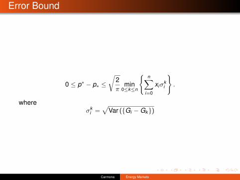
Error Bound
0 ≤ p∗ − p∗ ≤√
2π
min0≤k≤n
{n∑
i=0
xiσki
}.
whereσk
i =√
Var ({Gi −Gk})
Carmona Energy Markets

Numerical Performance
0.75 0.88 1.00 1.13 1.250
0.05
0.1
0.15
0.2
0.25
0.3
0.35
strike K
pric
e
ρ = 30% σ = 10%
0.75 0.88 1.00 1.13 1.250
0.05
0.1
0.15
0.2
0.25
0.3
0.35
strike K
pric
e
ρ = 30% σ = 20%
0.75 0.88 1.00 1.13 1.250
0.05
0.1
0.15
0.2
0.25
0.3
0.35
strike K
pric
e
ρ = 30% σ = 30%
0.75 0.88 1.00 1.13 1.250
0.05
0.1
0.15
0.2
0.25
0.3
0.35
strike K
pric
e
ρ = 50% σ = 10%
0.75 0.88 1.00 1.13 1.250
0.05
0.1
0.15
0.2
0.25
0.3
0.35
strike K
pric
e
ρ = 50% σ = 20%
0.75 0.88 1.00 1.13 1.250
0.05
0.1
0.15
0.2
0.25
0.3
0.35
strike K
pric
e
ρ = 50% σ = 30%
0.75 0.88 1.00 1.13 1.250
0.05
0.1
0.15
0.2
0.25
0.3
0.35
strike K
pric
e
ρ = 70% σ = 10%
0.75 0.88 1.00 1.13 1.250
0.05
0.1
0.15
0.2
0.25
0.3
0.35
strike K
pric
e
ρ = 70% σ = 20%
0.75 0.88 1.00 1.13 1.250
0.05
0.1
0.15
0.2
0.25
0.3
0.35
strike K
pric
e
ρ = 70% σ = 30%
FIGURE 1. Lower and upper bound on the price for a basket op-tion on 50 stocks (each one having a weight of1/50) as a functionof K. “+” denote Monte Carlo results.
Functionsuk for k = 10j with j = 1, 2, · · · , 25, x∗
∞would be.725.
1
Carmona Energy Markets
Asian Options2
0.75 0.88 1.00 1.13 1.250
0.05
0.1
0.15
0.2
0.25
0.3
0.35
strike K
pric
e
σ = 10%
0.75 0.88 1.00 1.13 1.250
0.05
0.1
0.15
0.2
0.25
0.3
0.35
strike K
pric
e
σ = 20%
0.75 0.88 1.00 1.13 1.250
0.05
0.1
0.15
0.2
0.25
0.3
0.35
strike K
pric
e
σ = 30%
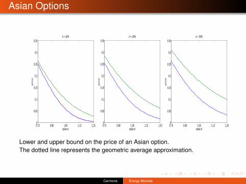
FIGURE 2. Lower and upper bound on the price of an Asian op-tion. The dotted line represents the geometric average approxima-tion.
values ofx∗
kcomputed fork = 1, 2, · · · , 250.
Lower and upper bound on the price of an Asian option.The dotted line represents the geometric average approximation.
Carmona Energy Markets

Computation of (Approximate) Greeks
∆∗i =∂p∗∂xi
= εiΦ(
d∗ + σi(√
Cv∗)i
)Vega∗i =
∂p∗∂σi
√T = εixi(
√Cv∗)iϕ
(d∗ + σi(
√Cv∗)i
)√T
χ∗ij =∂p∗∂ρij
=12
n∑k=0
εk xk
(σiC
− 12
kj v∗j + σjC− 1
2ki v∗i
)ϕ(
d∗ + σk (√
Cv∗)k
)Θ∗ =
∂p∗∂T
=1
2T
n∑k=0
εk xkσk (√
Cv∗)kϕ(
d∗ + σk (√
Cv∗)k
).
Carmona Energy Markets

Second Order Derivatives
Γ∗ij = εiεj
ϕ(
d∗ + σi(√
Cv∗)i
)ϕ(
d∗ + σj(√
Cv∗)j
)∑n
k=0 εk xkσk (√
Cv∗)kϕ(
d∗ + σk (√
Cv∗)k
) ,then
−Θ∗ +1
2T
n∑i=0
n∑j=0
ΣijxixjΓ∗ij = 0.
Carmona Energy Markets

Down-and-Out Call on a Basket of n Stocks
Option Payoff (n∑
i=1
wiSi(T )− K
)+
1{inft≤T S1(t)≥H}.
Option price is
E
(
n∑i=0
εixieGi (1)− 12 σ2
i 1{infθ≤1 x1eG1(θ)− 1
2 σ21θ≥H
})+ ,
whereε1 = +1, σ1 > 0 and H < x1
{G(θ); θ ≤ 1} is a (n + 1)-dimensional Brownian motion startingfrom 0 with covariance Σ.
Carmona Energy Markets

Price and Hedges
Use lower bound.
p∗ = supd,u
E
{n∑
i=0
εixieGi (1)− 12 σ2
i 1{infθ≤1 x1eG1(θ)− 1
2 σ21θ≥H;u·G(1)≤d
}}.
Girsanov implies
p∗ = supd,u
n∑i=0
εixiP{
infθ≤1
G1(θ)
+(Σi1 − σ2
1/2)θ ≥ ln
(Hx1
); u ·G(1) ≤ d − (Σu)i
}.
Carmona Energy Markets

Numerical Results
σ ρ H/x1 n = 10 n = 20 n = 300.4 0.5 0.7 0.1006 0.0938 0.09390.4 0.5 0.8 0.0811 0.0785 0.07770.4 0.5 0.9 0.0473 0.0455 0.04490.4 0.7 0.7 0.1191 0.1168 0.11650.4 0.7 0.8 0.1000 0.1006 0.09950.4 0.7 0.9 0.0608 0.0597 0.05940.4 0.9 0.7 0.1292 0.1291 0.12900.4 0.9 0.8 0.1179 0.1175 0.11730.4 0.9 0.9 0.0751 0.0747 0.07450.5 0.5 0.7 0.1154 0.1122 0.11100.5 0.5 0.8 0.0875 0.0844 0.08160.5 0.5 0.9 0.0518 0.0464 0.04580.5 0.7 0.7 0.1396 0.1389 0.13880.5 0.7 0.8 0.1103 0.1086 0.10800.5 0.7 0.9 0.0631 0.0619 0.06150.5 0.9 0.7 0.1597 0.1593 0.15920.5 0.9 0.8 0.1328 0.1322 0.13200.5 0.9 0.9 0.0786 0.0782 0.0780
Carmona Energy Markets

Valuing a Tolling Agreement
Stylized Version
Leasing an Energy AssetFossil Fuel Power PlantOil RefineryPipeline
Owner of the AgreementDecides when and how to use the asset (e.g. run the power plant)Has someone else do the leg work
Carmona Energy Markets

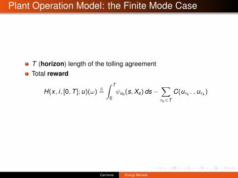
Plant Operation Model: the Finite Mode Case
Markov process (state of the world) Xt = (X (1)t ,X (2)
t , · · · )(e.g. X (1)
t = Pt , X (2)t = Gt , X (3)
t = Ot for a dual plant)
Plant characteristicsZM
M= {0, · · · ,M − 1} modes of operation of the plant
H0,H1 · · · ,HM−1 heat rates{C(i , j)}(i,j)∈ZM regime switching costs (C(i , j) = C(i , `) + C(`, j))ψi(t , x) reward at time t when world in state x , plant in mode i
Operation of the plant (control) u = (ξ, T ) whereξk ∈ ZM
M= {0, · · · ,M − 1} successive modes
0 6 τk−1 6 τk 6 T switching times
Carmona Energy Markets
Plant Operation Model: the Finite Mode Case
T (horizon) length of the tolling agreementTotal reward
H(x , i , [0,T ]; u)(ω)M=
∫ T
0ψus(s,Xs) ds −
∑τk <T
C(uτk−,uτk )
Carmona Energy Markets

Stochastic Control Problem
U(t)) acceptable controls on [t ,T ](adapted cadlag ZM -valued processes u of a.s. finite variation on [t ,T ])
Optimal Switching Problem
J(t , x , i) = supu∈U(t)
J(t , x , i ; u),
where
J(t , x , i ; u) = E[H(x , i , [t ,T ]; u)|Xt = x ,ut = i
]= E
[∫ T
0ψus(s,Xs) ds −
∑τk <T
C(uτk−,uτk )|Xt = x ,ut = i]
Carmona Energy Markets
Iterative Optimal Stopping
Consider problem with at most k mode switches
Uk (t) M= {(ξ, T ) ∈ U(t) : τ` = T for ` > k + 1}
Admissible strategies on [t ,T ] with at most k switches
Jk (t , x , i) M= esssupu∈Uk (t)E
[∫ T
tψus (s,Xs) ds−
∑t6τk <T
C(uτk−, uτk )∣∣∣Xt = x , ut = i
].
Carmona Energy Markets

Alternative Recursive Construction
J0(t , x , i) M= E
[∫ T
tψi(s,Xs) ds
∣∣∣Xt = x],
Jk (t , x , i) M= sup
τ∈St
E[∫ τ
tψi(s,Xs) ds +Mk,i(τ,Xτ )
∣∣∣Xt = x].
Intervention operator M
Mk,i(t , x)M= max
j 6=i
{−Ci,j + Jk−1(t , x , j)
}.
Hamadene - Jeanblanc (M=2)
Carmona Energy Markets
Variational Formulation
NotationLX X space-time generator of Markov process Xt in Rd
Mφ(t , x , i) = maxj 6=i{−Ci,j + φ(t , x , j)} intervention operator
Assumeφ(t , x , i) in C1,2(([0,T ]× Rd) \D
)∩ C1,1(D)
D = ∪i{(t , x) : φ(t , x , i) = Mφ(t , x , i)
}(QVI) for all i ∈ ZM :
1 φ > Mφ,2 Ex[∫ T
0 1φ6Mφ dt]
= 0,3 LXφ(t , x , i) + ψi(t , x) 6 0, φ(T , x , i) = 0,4
(LXφ(t , x , i) + ψi(t , x)
)(φ(t , x , i)−Mφ(t , x , i)
)= 0.
Conclusion
φ is the optimal value function for the switching problem
Carmona Energy Markets

Reflected Backward SDE’s
AssumeX0 = x & ∃(Y x ,Z x ,A) adapted to (FX
t )
E[
sup06t6T
|Y xt |2 +
∫ T
0‖Z x
t ‖2 dt + |AT |2]<∞
and
Y xt =
∫ T
tψi(s,X x
s ) ds + AT − At −∫ T
tZs · dWs,
Y xt > Mk,i(t ,X x
t ),∫ T
0(Y x
t −Mk,i(t ,X xt )) dAt = 0, A0 = 0.
Conclusion: if Y x0 = Jk (0, x , i) then
Y xt = Jk (t ,X x
t , i)
Carmona Energy Markets
System of Reflected Backward SDE’s
QVI for optimal switching: coupled system of reflected BSDE’s for(Y i)i∈ZM ,
Y it =
∫ T
tψi(s,Xs) ds + Ai
T − Ait −∫ T
tZ i
s · dWs,
Y it > max
j 6=i{−Ci,j + Y j
t }.
Existence and uniqueness Directly for M > 2?M = 2, Hamadene - Jeanblanc use difference process Y 1 − Y 2.
Carmona Energy Markets

Discrete Time Dynamic Programming
Time Step ∆t = T/M]
Time grid S∆ = {m∆t , m = 0,1, . . . ,M]}Switches are allowed in S∆
DPP
For t1 = m∆t , t2 = (m + 1)∆t consecutive times
Jk (t1,Xt1 , i) = max(
E[∫ t2
t1
ψi(s,Xs) ds + Jk (t2,Xt2 , i)| Ft1
], Mk,i(t1,Xt1)
)'(ψi(t1,Xt1)∆t + E
[Jk (t2,Xt2 , i)| Ft1
])∨(
maxj 6=i
{−Ci,j + Jk−1(t1,Xt1 , j)
}).
(1)
Tsitsiklis - van Roy
Carmona Energy Markets

Longstaff-Schwartz VersionRecall
Jk (m∆t , x , i) = E[ τk∑
j=m
ψi(j∆t ,Xj∆t) ∆t +Mk,i(τ k∆t ,Xτk ∆t)∣∣Xm∆t = x
].
Analogue for τ k :
τ k (m∆t , x`m∆t , i) =
{τ k ((m + 1)∆t , x`
(m+1)∆t , i), no switch;m, switch,
(2)
and the set of paths on which we switch is given by {` : `(m∆t ; i) 6= i} with
`(t1; i) = arg maxj
(−Ci,j + Jk−1(t1, x`
t1 , j), ψi(t1, x`t1)∆t + Et1
[Jk (t2, ·, i)
](x`
t1)).
(3)
The full recursive pathwise construction for Jk is
Jk (m∆t , x`m∆t , i) =
{ψi(m∆t , x`
m∆t) ∆t + Jk ((m + 1)∆t , x`(m+1)∆t , i), no switch;
−Ci,j + Jk−1(m∆t , x`m∆t , j), switch to j .
(4)
Carmona Energy Markets

Remarks
Regression used solely to update the optimal stopping times τ k
Regressed values never storedHelps to eliminate potential biases from the regression step.
Carmona Energy Markets

Algorithm
1 Select a set of basis functions (Bj) and algorithm parameters∆t ,M],Np, K , δ.
2 Generate Np paths of the driving process: {x`m∆t , m = 0, 1, . . . ,M],
` = 1, 2, . . . ,Np} with fixed initial condition x`0 = x0.
3 Initialize the value functions and switching times Jk (T , x`T , i) = 0,
τ k (T , x`T , i) = M] ∀i , k .
4 Moving backward in time with t = m∆t , m = M], . . . , 0 repeat the Loop:
Compute inductively the layers k = 0, 1, . . . , K (evaluateE[Jk (m∆t + ∆t , ·, i)| Fm∆t
]by linear regression of
{Jk (m∆t + ∆t , x`m∆t+∆t , i)} against {Bj(x`
m∆t)}NB
j=1, then add thereward ψi(m∆t , x`
m∆t) ·∆t)Update the switching times and value functions
5 end Loop.
6 Check whether K switches are enough by comparing J K and J K−1 (theyshould be equal).
Observe that during the main loop we only need to store the bufferJ(t , ·), . . . , J(t + δ, ·); and τ(t , ·), · · · , τ(t + δ, ·).
Carmona Energy Markets

Convergence
Bouchard - TouziGobet - Lemor - Warin
Carmona Energy Markets

Example 1
dXt = 2(10− Xt) dt + 2 dWt , X0 = 10,
Horizon T = 2,Switch separation δ = 0.02.Two regimesReward rates ψ0(Xt) = 0 and ψ1(Xt) = 10(Xt − 10)
Switching cost C = 0.3.
Carmona Energy Markets

Value Functions
0 0.5 1 1.5 20
1
2
3
4
5
6
7
8
9
Years to maturity
Value
Fun
ction
for s
ucce
ssive
k
Jk (t , x ,0) as a function of t
Carmona Energy Markets
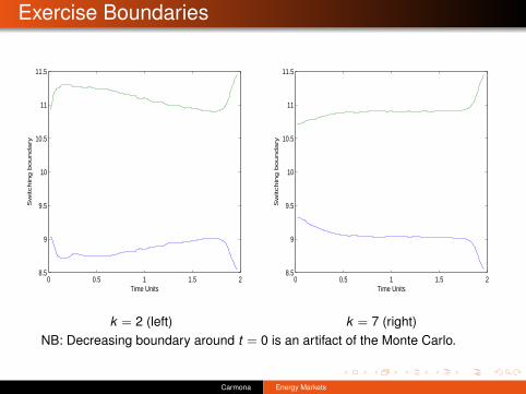
Exercise Boundaries
0 0.5 1 1.5 28.5
9
9.5
10
10.5
11
11.5
Time Units
Sw
itch
ing
bo
un
da
ry
0 0.5 1 1.5 28.5
9
9.5
10
10.5
11
11.5
Time Units
Sw
itch
ing
bo
un
da
ry
k = 2 (left) k = 7 (right)NB: Decreasing boundary around t = 0 is an artifact of the Monte Carlo.
Carmona Energy Markets
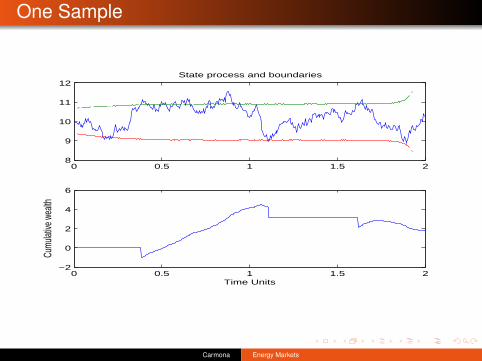
One Sample
0 0.5 1 1.5 2−2
0
2
4
6
Time Units
Cumu
lative
wea
lth
0 0.5 1 1.5 28
9
10
11
12State process and boundaries
Carmona Energy Markets
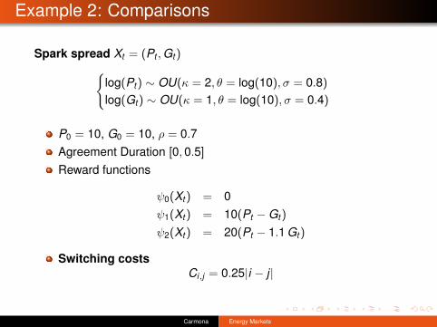
Example 2: Comparisons
Spark spread Xt = (Pt ,Gt){log(Pt) ∼ OU(κ = 2, θ = log(10), σ = 0.8)
log(Gt) ∼ OU(κ = 1, θ = log(10), σ = 0.4)
P0 = 10, G0 = 10, ρ = 0.7Agreement Duration [0,0.5]
Reward functions
ψ0(Xt) = 0ψ1(Xt) = 10(Pt −Gt)
ψ2(Xt) = 20(Pt − 1.1 Gt)
Switching costsCi,j = 0.25|i − j |
Carmona Energy Markets

Numerical Comparison
Method Mean Std. Dev Time (m)Explicit FD 5.931 − 25LS Regression 5.903 0.165 1.46TvR Regression 5.276 0.096 1.45Kernel 5.916 0.074 3.8Quantization 5.658 0.013 400∗
Table: Benchmark results for Example 2.
Carmona Energy Markets
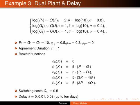
Example 3: Dual Plant & Delay
log(Pt) ∼ OU(κ = 2, θ = log(10), σ = 0.8),
log(Gt) ∼ OU(κ = 1, θ = log(10), σ = 0.4),
log(Ot) ∼ OU(κ = 1, θ = log(10), σ = 0.4), .
P0 = G0 = O0 = 10, ρpg = 0.5,ρpo = 0.3, ρgo = 0
Agreement Duration T = 1
Reward functions
ψ0(Xt) ≡ 0
ψ1(Xt) = 5 · (Pt −Gt)
ψ2(Xt) = 5 · (Pt −Ot),
ψ3(Xt) = 5 · (3Pt − 4Gt)
ψ4(Xt) = 5 · (3Pt − 4Ot).
Switching costs Ci,j ≡ 0.5
Delay δ = 0, 0.01, 0.03 (up to ten days)
Carmona Energy Markets

Numerical Results
Setting No Delay δ = 0.01 δ = 0.03Base Case 13.22 12.03 10.87Jumps in Pt 23.33 22.00 20.06
Regimes 0-3 only 11.04 10.63 10.42Regimes 0-2 only 9.21 9.16 9.14Gas only: 0,1,3 9.53 7.83 7.24
Table: LS scheme with 400 steps and 16000 paths.
RemarksHigh δ lowers profitability by over 20%.
Removal of regimes: without regimes 3 and 4 expected profit drops from13.28 to 9.21.
Carmona Energy Markets

Example 4: Exhaustible ResourcesInclude It current level of resources left (It non-increasing process).
J(t , x , c, i) = supτ,j
E[∫ τ
tψi(s,Xs) ds + J(τ,Xτ , Iτ , j)− Ci,j |Xt = x , It = c
].
(5)
� Resource depletion (boundary condition) J(t , x ,0, i) ≡ 0.� Not really a control problem It can be computed on the fly
Mining example of Brennan and Schwartz varying the initialcopper price X0
Method/ X0 0.3 0.4 0.5 0.6 0.7 0.8BS ’85 1.45 4.35 8.11 12.49 17.38 22.68
PDE FD 1.42 4.21 8.04 12.43 17.21 22.62RMC 1.33 4.41 8.15 12.44 17.52 22.41
Carmona Energy Markets

Extension to Gas Storage & Hydro Plants
Accomodate outagesInclude switch separation as a form of delayWas extended (R.C. - M. Ludkovski) to treat
Gas StorageHydro Plants
Porchet-Touzi
Carmona Energy Markets
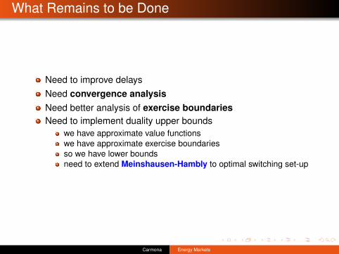
What Remains to be Done
Need to improve delaysNeed convergence analysisNeed better analysis of exercise boundariesNeed to implement duality upper bounds
we have approximate value functionswe have approximate exercise boundariesso we have lower boundsneed to extend Meinshausen-Hambly to optimal switching set-up
Carmona Energy Markets

Financial Hedging
Extending the Analysis Adding Access to a Financial Market
Porchet-Touzi
Same (Markov) factor process Xt = (X (1)t ,X (2)
t , · · · ) as beforeSame plant characteristics as beforeSame operation control u = (ξ, T ) as beforeSame maturity T (end of tolling agreement) as beforeReward for operating the plant
H(x , i ,T ; u)(ω)M=
∫ T
0ψus(s,Xs) ds −
∑τk <T
C(uτk−,uτk )
Carmona Energy Markets

Hedging/Investing in Financial Market
Access to a financial market (possibly incomplete)y initial wealthπt investment portfolioY y,π
T corresponding terminal wealth from investmentUtility function U(y) = −e−γy
Maximum expected utility
v(y) = supπ
E{U(Y y,πT )}
Carmona Energy Markets
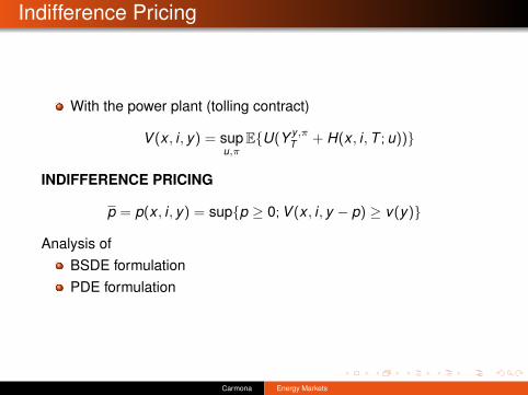
Indifference Pricing
With the power plant (tolling contract)
V (x , i , y) = supu,π
E{U(Y y,πT + H(x , i ,T ; u))}
INDIFFERENCE PRICING
p = p(x , i , y) = sup{p ≥ 0; V (x , i , y − p) ≥ v(y)}
Analysis ofBSDE formulationPDE formulation
Carmona Energy Markets
Recommended


![[Derivatives Consulting Group] Introduction to Equity Derivatives](https://img.pdfslide.us/doc/110x75/5525eed15503467c6f8b4b12/derivatives-consulting-group-introduction-to-equity-derivatives.jpg)