Energy Finite Element Analysis Developments for High Frequency
Vibration Analysis of Composite Structures
by
Xiaoyan Yan
A dissertation submitted in partial fulfillment of the requirements for the degree of
Doctor of Philosophy (Naval Architecture and Marine Engineering)
in The University of Michigan 2008
Doctoral Committee: Professor Nickolas Vlahopoulos, Co-Chair Assistant Research Scientist Aimin Wang, Co-Chair Professor Michael M. Bernitsas Professor Anthony M. Waas Associate Research Scientist Matthew P. Castanier

© Reserved Rights All
YanXiaoyan 2008

ii
To my parents Baolin Yan and Ruijuan Cao
without whose sacrifices none of this would be possible.

iii
ACKNOWLEDGMENTS
This dissertation is the result of three and half years of work whereby I have been
accompanied, supported and encouraged by many people. It is a pleasant aspect that I
have now the opportunity to express my gratitude to all of them.
First and foremost, I would like to express my deep and sincere gratitude to my
advisor, Professor Nickolas Vlahopoulos, for his support, patience and encourgment
throughout my research and study at the University of Michigan. His expertise and
technical knowledge is essential to the completion of this dissertation and has taught me
innumerable lessons and insights in research.
I would like to sincerely thank Dr. Aimin Wang for giving me consistent guidance
and advices to my research and for being the co-chair of my committee. He always finds
time to oversee my research and to share his knowledge and expertise with me despite of
his busy schedule. This work wouldn’t have been possible without the encourgment and
support from him.
I would like to thank Professor Anthony M. Waas for being a member of my
committee and for monitoring my work and providing me with valuable comments on my
research. I leared a lot of knowledge on composite materials from him.
I appreciate the advice of my other dissertation committee members, Professor
Michael M. Bernitsas and Dr. Matthew Castanier. Thank them for giving valuable
comments on my dissertation.
I would like to acknowledge a numer of my friends and colleagues, without whom
this experience would have been incomplete. First, special thanks to my friends at the
University of Michigan, who have made my life and study here an unforgettable

iv
experience. Some of them are: James Bretl, Jim Chang, Jinting Guo, Sina
Hassanaliaragh, Elisha Garcia, Zheyu Hong, Jonghun Lee, Yaning Li, Zhen Li, Sai
Mohan Majhi, Javid Moraveji, Ellie Nick, Varun Raghunathan, Oscar Tascon, Hui Tang,
Zhigang Tian, Wei Wu, Handa Xi, Yanhui Xie. Thanks also due to my colleagues and
friends in Houston:, Steven Barras, Nicole Liu, Yang Mu, Xinguo Ning, Jiulong Sun, Jim
Wang, Jin Wang, Xiaoning Wang and Lixin Xu. I would also like to thank my best
friends, Rong Wu, Ying Jin and Bei Lu, for their continuous encouragement and
accompany through the three and half years and for giving me a great time studying in
Michigan.
I would like to thank my closest friend Kamaldev Raghavan, who gave me
consistent support and encourgment throughout my Ph.D. study.
This research was supported by the Automotive Research Center, a U.S. Army
RDECOM center of excellence for modeling and simulation of ground vehicles led by
the University of Michigan.
I would also like to thank and the department of Naval Architecture and Marine
Engineering, University of Michigan and the Barbour Scholarship for their fellowships
and support during my graduate study.

v
TABLE OF CONTENTS
DEDICATION................................................................................................................... ii
ACKNOWLEDGMENTS ............................................................................................... iii
LIST OF FIGURES ....................................................................................................... viii
ABSTRACT ........................................................................................................................x
CHAPTER 1 INTRODUCTION ..................................................................................... 1
1.1 RESEARCH OVERVIEW ................................................................................ 1
1.2 LITERATURE REVIEW ................................................................................. 4
1.2.1 Finite Element Analysis and composite materials ................. 4 1.2.2 Statistical Energy Analysis .................................................... 8 1.2.3 Energy Finite Element Analysis .......................................... 11 1.2.4 Power transmission through joints ....................................... 15
1.3 DISSERTATION CONTRIBUTION............................................................. 20
1.4 DISSERTATION OVERVIEW ...................................................................... 22
CHAPTER 2 BACKGROUND OF ENERGY FINITE ELEMENT ANALYSIS ...................................................................................................................... 25
2.1 INTRODUCTION............................................................................................ 25
2.2 EFEA DEVELOPMENTS FOR A SINGLE ISOTROPIC PLATE ........... 25
2.3 EFEA DEVELOPMENTS FOR ISOTROPIC PLATE JUNCTIONS ....... 29
2.4 EXAMPLE OF PREVIOUS EFEA APPLICATIONS ................................ 31
CHAPTER 3 EFEA DEVELOPMENTS IN SINGLE COMPOSITE LAMINATE PLATE ...................................................................................................... 33
3.1 INTRODUCTION............................................................................................ 33
3.2 SYNTHESIS OF STIFFNESS MATRIX FOR COMPOSITE LAMINATE PLATES ............................................................................... 35
3.2.1 Stress-strain relation for generally orthotropic lamina ........ 35 3.2.2 Synthesis of stiffness matrix for composite laminate
plates ....................................................................................... 37
vi
3.3 GOVERNING EQUATIONS FOR THE VIBRATION OF COMPOSITE LAMINATE PLATES ..................................................... 39
3.4 EFEA DEVELOPMENT FOR THE FLEXURAL WAVES IN COMPOSITE LAMINATE PLATES ..................................................... 43
3.4.1 Wave solution of displacement and the dispersion relation for flexural waves ...................................................... 43
3.4.2 Derivation of time- and space- averaged energy density and intensities.......................................................................... 45
3.4.3 Derivation of EFEA differential equation and its variational statement ............................................................... 47
3.5 EFEA DEVELOPMENT FOR THE IN-PLANE WAVES IN COMPOSITE LAMINATE PLATES ..................................................... 51
3.5.1 Displacement solution the dispersion relationship for in-plane waves ........................................................................ 51
3.5.2 Derivation of time- and space- averaged energy density and intensities.......................................................................... 53
3.5.3 Derivation of EFEA differential equations for in-plane motions .................................................................................... 55
3.6 NUMERICAL EXAMPLES AND VALIDATION ....................................... 56 3.6.1 Two-layer cross-ply laminate plate ...................................... 57 3.6.2 Two-layer general laminate plate ......................................... 63
3.7 AN ALTERNATIVE METHOD TO DERIVE THE EFEA DIFFERENTIAL EQUATION FOR COMPOSITE LAMINATE PLATES ...................................................................................................... 68
3.7.1Group velocity for composite laminate plates ...................... 68 3.7.2 Equivalent homogenized isotropic material for
composite laminate plates ....................................................... 70 3.7.3 Validation of alternative approach ....................................... 71
CHAPTER 4 POWER TRANMISSION THROUGH COUPLED ORTHOTROPIC PLATES............................................................................................ 73
4.1 INTRODUCTION............................................................................................ 73
4.2 DERIVATION OF POWER TRANSMISSION COEFFICIENTS FOR ORTHOTROPIC PLATE JUNCTION ......................................... 75
4.2.1 Governing equations ............................................................ 75 4.2.2 Derivation of in-plane wavenumbers for orthotropic
plates ....................................................................................... 77 4.2.3 Derivation of dynamic stiffness matrix ................................ 79 4.2.4 Assembly of the complete equations and the calculation
of transmission coefficients .................................................... 84 4.3 DERIVATION OF JOINT MATRIX ............................................................ 86
4.3.1 Power flow relationship of two systems through a lossless joint ............................................................................ 86
vii
4.3.2 Joint matrix for two coupled plates ...................................... 89 4.4 ASSEMBLY OF GLOBAL MATRIX FOR COUPLED
ORTHOTROPIC PLATES....................................................................... 90
4.5 NUMERICAL EXAMPLES AND VALIDATION ....................................... 91
CHAPTER 5 POWER TRANMISSION THROUGH COUPLED COMPOSITE LAMINATE PLATES ........................................................................ 100
5.1 INTRODUCTION.......................................................................................... 100
5.2 DERIVATION OF POWER TRANSMISSION COEFFICIENTS .......... 101 5.2.1 Governing equations .......................................................... 101 5.2.2 Derivation of in-plane wavenumbers for composite
laminate plates ...................................................................... 102 5.2.3 Derivation of dynamic stiffness matrix .............................. 103 5.2.4 Assembly of the complete equations and the calculation
of transmission coefficients .................................................. 107 5.3 DERIVATION OF JOINT MATRIX .......................................................... 108
5.4 ASSEMBLY OF GLOBAL EFEA EQUATIONS FOR COUPLED COMPOSITE LAMINATE PLATES ................................................... 108
5.5 NUMERICAL EXAMPLES AND VALIDATION ..................................... 109
CHAPTER 6 CONCLUSIONS AND RECOMMENDATIONS FOR FUTURE WORK .......................................................................................................... 116
6.1 CONCLUSIONS ............................................................................................ 116
6.2 RECOMMENDATIONS FOR FUTURE WORK ...................................... 118
APPENDIX .................................................................................................................... 120
REFERENCES .............................................................................................................. 125

viii
LIST OF FIGURES
Figure 2.1 EFEA results for the flexural energy in a vehicle due to track excitation ....... 31
Figure 2.2 Conventional FEA and EFEA model for an Army vehicle ............................. 32
Figure 3.1 Construction of composite laminate plate ....................................................... 35
Figure 3.2 Two coordinates of a generally orthotropic lamina ......................................... 36
Figure 3.3 Geometry of multilayered laminate ................................................................. 38
Figure 3.4 Exact and approximate frequencies for the angle-ply laminate plate .............. 42
Figure 3.5 Input power comparison between FEA and analytic solutions ....................... 50
Figure 3.6 Configuration of two-layer cross-ply laminate plate ....................................... 57
Figure 3.7 Conventional FEA model (left) and EFEA model (right) ............................... 58
Figure 3.8 Distribution of energy density along the mid-span of the cross-ply laminate
plate computed by the dense FEA and EFEA models at 1000Hz-5000Hz 1/3 octave bands
........................................................................................................................................... 62
Figure 3.9 Configuration of composite laminate plate ..................................................... 63
Figure 3.10 Distribution of energy density along the mid-span of the general laminate
plate computed by the dense FEA and EFEA models at 1000Hz-5000Hz 1/3 octave bands
........................................................................................................................................... 67
Figure 3.11 Wavenumber as a function of wave heading in the wavenumber plane ....... 68
Figure 3.12 Energy density distribution comparison between composite laminate plate
and its equivalent isotropic plate ....................................................................................... 72
Figure 4.1 Schematic of plate junction ............................................................................. 74
ix
Figure 4.2 Coordinate system, displacements, forces and moments for plate j ................ 76
Figure 4.3 Schematic plot of energy flow between two subsystems for a single wave .... 86
Figure 4.4 Four different orientations for two orthotropic plate L-junctions ................... 92
Figure 4.5 The transmission loss for the four cases of orthotropic L-junction ................. 93
Figure 4.6 The models of orthotropic L-junction in conventional FEA and EFEA ......... 94
Figure 4.7 Energy density in two orthotropic plates (t=0.01m) ........................................ 96
Figure 4.8 Energy density in two orthotropic plates (t=0.001m) ...................................... 99
Figure 5.1 The orientation of the first composite laminate plate .................................... 110
Figure 5.2 The orientation of the second composite laminate plate ............................... 110
Figure 5.3 The models of orthotropic L-junction in conventional FEA and EFEA ....... 111
Figure 5.4 Comparison of energy density between EFEA and conventional FEA (case 1)
......................................................................................................................................... 112
Figure 5.5 Comparison of energy density between EFEA and conventional FEA (case 2)
......................................................................................................................................... 113
Figure 5.6 Comparison of velocity difference between two plates (case 1) ................... 114
Figure 5.7 Comparison of velocity difference between two plates (case 2) ................... 114

x
ABSTRACT
Energy finite element analysis (EFEA) has been proven to be an effective and
reliable tool for high frequency vibration analysis. It uses the averaged energy density as
the primary variable to form the governing differential equations and provides a practical
approach to evaluate the structural response at high frequencies, which is hard to reach
with conventional finite element analysis because of the computational cost. In the past,
EFEA has been applied successfully to different structures, such as beams, rods, plates,
curved panels etc. Until recently, however, not much work has been done in the field of
composite structures.
Research for developing a new EFEA formulation for modeling composite
laminate plates is presented in this dissertation. The EFEA governing differential
equation, with the time- and space- averaged energy density as the primary variable, is
developed for general composite laminate plates. The power transmission characteristics
at plate junctions of non-isotropic materials, including orthotropic plates and composite
laminate plates are studied in order to obtain the power transmission coefficients at the
junction. These coefficients are utilized to compute the joint matrix that is needed to
assemble the global system of EFEA equations. The global system of EFEA equations
can be solved numerically and the energy density distribution within the entire system
can then be obtained. The results from the EFEA formulation have been validated
through comparison with results from very dense FEA models.

1
Chapter 1
INTRODUCTION
1.1 Research Overview
Composite materials are formed by combining two or more materials that have
quite different properties. The different materials work together to give the composite
unique properties. The greatest advantage of composite materials is strength and stiffness
combined with lightness. Because of these advantages, composite laminate plate and
shell structures are being increasingly used as primary structural components in
applications where weight saving is of critical concern, such as automotive, aerospace
and naval architecture industries.
One of the applications of composite materials is that they can be used for the
construction of army vehicles to make them lightweight. However, at the same time, the
use of composite materials makes the vehicles structures more vulnerable to dynamic and
shock loads. Due to the short duration of shock events, the high frequency content of the
loads is responsible for the transfer of power from the location of the excitation to the
location where sensitive electronic equipment is mounted. To improve the performance
of composite materials under impact and utilize them to their full advantage, it is crucial
to have a good understanding of their response under impact loads.

2
The frequency spectrum where simulation methods can be utilized for vibration
analysis can be divided into three regions: low, mid and high frequency. The low
frequency region is defined as the frequency range where all components are short
compared to the wavelength. Finite Element Analysis (FEA) simulations are used for
computing the response of structures at low frequency. In the mid-frequency range, the
system is comprised of both long and short members. The method of combining SEA or
EFEA with conventional finite element analysis was used to simulate the vibration
response at mid frequencies.
The high frequency range is defined as the frequency range where all component
member of a system are long compared to the wavelength. At high frequency,
conventional FEA methods require a very large number of elements in order to capture
the high frequency characteristic of the structures, which results in very high
computational costs. Statistical Energy Analysis (SEA) and Energy Finite Element
Analysis (EFEA) are the two developments for high frequency vibration analysis.
In SEA, the system is partitioned into coupled “subsystems” of similar modes and
the stored and exchanged energies in each “subsystem” are analyzed through a set of
linear equations. The primary variable in SEA is the lumped averaged energy in each
subsystem. A subsystem can be seen as a part or physical element of the structure that is
analyzed. To be modeled as a subsystem, the part or element should be able to vibrate
quite independently from other elements and a reverberant sound field should exist with
the subsystem. If different wave types exist in the element, then each of the
corresponding sound field is modeled as one subsystem. In general, a subsystem is a

3
group of similar energy storage modes. In SEA, the “statistical” operation is represented
by the frequency, spatial and ensemble average over a group of modes.
EFEA is a recently developed finite element approach for high frequency
vibration and acoustic analysis. In EFEA, the energy density is defined as the primary
variable. The governing differential equation is developed in terms of energy density and
numerical solution is employed using finite element approach. It can capture the vibration
property of the structure by using a significantly smaller number of elements compared to
conventional FEA methods. The EFEA has been utilized in modeling automotives,
marine structures and aircrafts etc. It has been validated through comparison to results
from very dense FEA models and test data.
Compared to SEA, the advantages of EFEA are that it can provide the detail
energy distribution within the subsystems and it can also take into consideration of the
local damping effects within the subsystems. Furthermore, it is possible to use the
existing models in conventional FEA in the EFEA method.
Until recently, most of the research on EFEA is related to isotropic materials,
where the material properties are the same at all the directions. Some work had been
done in orthotropic plates where the properties are different in two perpendicular
directions. Until recently, not much work has been done in the field of composite plates.
In order to extend the EFEA developments for composite materials, it is necessary to
derive the more general EFEA differential equations for composite materials.
In this dissertation, the EFEA differential equation for composite laminate plates
is developed. The derivation follows the same procedure as the development of EFEA in
isotropic materials. First, the equations of motion for composite laminate plate are

4
obtained. The relationship between the time- and space-averaged energy density and
energy intensities are found in order to establish the EFEA governing differential
equations for general composite laminate plates. A variational form is employed to solve
the EFEA differential equation. The energy density distribution of the composite laminate
plates obtained from EFEA formulation is compared and validated with very dense FEA
models of the plates. Then, for the coupled composite laminate plates, the power
transmission coefficient at the junction is derived by utilizing the wave propagating
method. The dynamic stiffness matrix for each plate is derived and the equations of
motion of the junction are obtained by applying the appropriate equilibrium and
compatibility conditions. The power transmission coefficients are calculated by solving
the equations of motion at the junction. At last, the joint matrix at the junction is
calculated and the global system of EFEA equation is established. The primary variable
of the equation – energy density can then be calculated.
1.2 Literature Review
1.2.1 Finite Element Analysis and composite materials
In the past, conventional finite element analysis has been employed to evaluate
the response of the structural system to the dynamic loads. The FEA formulation can be
used to analyze arbitrary complex structures. It considers the continuous structures as a
number of elements that connected to each other by the compatibility and equilibrium
conditions. However, because of the necessity of obtaining the element size much smaller
(typically 1/6) than the wavelength, FEA requires small meshes to describe the rapidly
changing modes of the structures(Kim, Kang et al. 1994). Thus, FEA is mainly limited to
analyzing the vibration at relatively low frequencies.

5
However, a number of researches have been done on the application of finite
element analysis to the high frequency response of composite structures subject to
impact/shock loads.
A transient dynamic finite element model was developed to analyze the response
of a laminated composite plate subject to a foreign object impact in order to examine the
susceptibility to impact of fiber-reinforced laminated composites that have been widely
used in aerospace structures (Wu and Chang 1989). Instead of using two-dimensional
plate theories, they studied the stress and strain distributions through the laminate
thickness during the impact. A correlation was found between the strain energy density
distributions and the resultant impact damage from the results.
A super finite element method was employed to predict the transient response of
laminated composite plates and cylindrical shells subject to impact loads (Vaziri, Quan et
al. 1996). The results were compared with experimental date and theoretical solutions.
The super element technique was proved to be a simple and efficient method to predict
the response of laminated composite plates and shells under impact loading although its
limited applicability due to the linear elastic material behavior assumption.
The response of a fiber-reinforced composite laminate plate subject to central
impact was investigated (Oguibe and Webb 1999). The failure mode was approximated
by the model combining spring, gap and dashpot elements that account for the energy
dissipated during the damage process. The numerical results were compared with the
experimental data and good agreements were observed. It was concluded that the
coupling between the dynamic response and stiffness degradation due to damage must be
considered in order to predict correctly the damage due to impact. This dynamic finite

6
element model, together with the failure algorithm, can be used as a good numerical tool
to predict the response of composite structures under impact loads.
A new weighted homogenization method was introduced for the design analysis
of composite laminate structures for light weight armored vehicles (Rostam-Abadi, Chen
et al. 2000). The method is modified from the standard homogenization method by
applying the weighted material constants of the laminae in order to reflect the nature of
beding. Numerical examples were presented using finite element analysis and the method
was validated with classical lamination theory and first-order shear deformation theory.
The response of a laminated composite cylindrical shell was calculated by the
classical Fourier series and the finite element method (Krishnamurthy, Mahajan et al.
2003). The analytical method provides information to help select appropriate mesh and
time step sizes for finite element method. A spectral finite element model was developed
to study the effect of wave scattering and power flow in composite beams with general
ply stacking sequence (Mahapatra and Gopalakrishnan 2004).
The composite laminate and shell structures subject to low velocity impact were
studied by Her and Liang (Her and Liang 2004) using ANSYS/LSDYNA finite element
software. The impact force was modeled by the modified Hertz contact law. The effects
of various parameters were examined in the parametric study.
The damage of a range of sandwich panels under impact loads was examine using
experimental investigation and numerical simulation (Meo, Vignjevic et al. 2005). The
numerical simulation was performed using transient dynamic finite element analysis code.
The load distribution in the damaged sandwich structure and the failure mechanism under
the impact load were examined.

7
The dynamic analysis of shell structures, with emphasis on application to steel
and steel-concrete composite blast resistant door was analyzed by Koh (Koh, Ang et al.
2003). An explicit integration method was adopted considering the short duration and
impulsive nature of the blast loading. Composite shell was handled by appropriate
integration rule across the thickness. Both material and geometric nonlinearities were
considered in the formulation.
The transient response of composite sandwich plates under initial stresses was
investigated using a new finite element formulation (Nayakl, Shenoi et al. 2006). The
new finite element formulation is based on a nine node assumed strain plate bending
element with nine degrees of freedom per node that developed from a refined high order
shear deformation theory.
A formulation of asymmetric laminated composite beam element that has super
convergence properties was presented (Chakraborty, Mahapatra et al. 2002). The
formulation is capable of capturing all the propagating wave modes at high frequencies
and can be utilized to solve the free vibration and wave propagation problems in
laminated composite beam structures. Qiu (Qiu, Deshpande et al. 2003) used the finite
element method to analyze the response of clamped sandwich beams subject to shock
loading and compared the results with analytical predictions.
Iannucci and Ankersen (Iannucci and Ankersen 2006) proposed an
unconventional energy based composite damage model that has been implemented into
the finite element codes for shell elements. In the model, the evolution of damage in each
mode (tensile, compressive and shear) was controlled via a set of damage-strain

8
equations to allow the total energy dissipated for each damage mode to be controlled
during impact event.
1.2.2 Statistical Energy Analysis
Statistical Energy Analysis (SEA) is developed based on the idea that at very high
frequencies the vibration problem is analogous to a thermal problem in which the
vibration energy density and damping are analogous to temperature and heat sinking
respectively. SEA has the advantage of reducing the order of governing differential
equations in vibratory analysis. In SEA, a large structure is reduced into smaller
subsystems which are coupled together through a set of linear equations. SEA is very
good in the study of sound and vibration transmission through complex structures at high
frequencies. However, it is not reliable at low frequencies due to the statistical
uncertainties that occur when there are few resonant modes in each of the subsystems.
The advantage of SEA is that it enables us to describe the subsystems more
simply by only a few physical parameters, such as the damping coefficients, modal
density, etc. (Lyon 1975). The disadvantage of SEA is that it gives statistical answers,
which are subject to some uncertainty. In this case, many of the systems may not have
enough modes in certain frequency bands to allow predictions with a high degree of
certainty.
The earliest work in the development of SEA were done in 1960s by Lyon and
Smith ((Lyon and Maidanik 1962; Smith 1962). In Lyon’s work (Lyon and Maidanik
1962), the interaction of a single mode of one system with many modes of another was
analyzed and an experimental study of a beam with a sound field was done. It also

9
showed the basic SEA parameters for the response prediction: modal density, damping
and coupling loss factor.
SEA has been applied to different types of systems. Following its initial
developments, the systems of plate and beam interaction and two plates connected
together were discussed (Lyon and Eichler 1964). The radiation of sound by reinforced
plates (Maidanik 1962) and the radiation of sound by cylinders (Manning and Maidanik
1964) were evaluated. SEA is also applied to other structures such as periodically
stiffened damped plate structures (Langley, Smith et al. 1997) that are widely used in
aerospace and marine vehicles.
Modal density is one of the important parameters in SEA. The development of
SEA motivated the effort in the evaluation of modal densities. The modal densities of
cylinders (Heckl 1962; Szecheny 1971) and curved panels (Wilkinson 1968) were
evaluated. The modal density of composite honeycomb sandwich panels is evaluated
(Renji, Nair et al. 1996). In the study, the expression for the modal density of honeycomb
sandwich panels with orthotropic face sheets was derived with the consideration of shear
flexibility of the core. The expression was verified by experiments and good agreement
was observed.
The modal density for the bending of anisotropic structural components was
studies by considering the case of periodic boundary conditions initially and then
extending to general boundary conditions (Langley 1996). The equation was validated
with empirical results.
Another important parameter of SEA is the coupling loss factor. It can be
computed using analytical (wave approach) or numerical methods (finite element

10
method). In the wave approach, the vibration of subsystems are represented by the
superposition of travelling waves, and coupling loss factor is evaluated by considering
the reflection and transmission at the junction (Fahy 1994).
The coupling loss factor for two coupled beams system was analyzed using two
methods: wave-transmission method and natural frequency-shift method (Crandali and
Lotz 1971) and the results from two methods are proved same for a particular system.
Langley (Langley 1989; Langley 1990) derived the expressions for the coupling loss
factor in terms of the frequency and space averaged Green functions on the assumption
that the coupling between the subsystems is conservative and weak coupling between the
subsystems.
Conventional finite element models were employed to determine the coupling loss
factors instead of analytical solutions when the connection between members presents a
complexity that cannot be accounted by analytical solutions. It is the only computational
option for calculating the power transfer characteristics for complex joints and
discontinuous joints. Simmons (Simmons 1991) calculated the SEA coupling loss factors
for L- and H- shape plate junctions using finite element methods at discrete frequencies
from 10 and 2000 Hz. The vibrational energy of the plates was calculated using FEA
instead of the traditional analytical solutions of an infinite junction between semi-infinite
plates. The space- and frequency- averaged solutions from FEA were found to be reliable
for calculating energy variables, although its calculation of displacement at individual
positions frequencies is not meaningful at high frequencies. Such averaged energies of
the plates can be used to derive the coupling loss factor of the junction that can be applied
to SEA of structures with the same type of junction. In another study (Fredo 1997), FEA

11
was combined with a SEA-like approach to obtain the power flow coefficients within a
system. The advantages of this approach include its ability of dealing with complicated
subsystem topologies, complicated joints, narrow bands frequencies and non-resonant
transmission mechanisms.
1.2.3 Energy Finite Element Analysis
Energy finite element analysis is an emerging new method for simulating high
frequency vibration response. It uses time- and space- averaged energy density as the
primary variable in the governing differential equations.
A power flow finite element analysis is presented by Nefske and Sung (Nefske
and Sung 1989). In their research, the new method was developed as an alterative to SEA
for high frequency vibration analysis. The formulation was based on power flow of a
differential control volume considering the conservation of energy. The partial
differential equation of the heat conduction type was derived and the finite element
approach was employed to solve the differential equation. The power flow finite element
model was formed by modifying a standard commercial structural finite element code. It
was shown that the same FEA model for predicting the vibration at low frequencies could
be modified to form the power flow finite element model for solving the vibration
problems at high frequencies for the same structural system.
Wohlever (Wohlever 1988; Wohlever and Bernhard 1992) investigated future the
thermal analogy to model mechanical power in structural acoustic systems. Energy
density equations were derived from the classical displacement solutions for
harmonically excited, hysteretically damped rods and beams. For the lightly damped rod,
the relationship between the local power and the local gradient of energy density can be

12
found. For the beam, however, this relationship can only be found if locally space
averaged values of power and energy density were utilized. This relationship, along with
the energy balance on a differential control volume, led to the development of a second
order equation that models the distribution of energy density in the structure. They also
investigated the coupling of energy for rods and beams. Two existing techniques – the
wave transmission approach and the receptance method were discussed and a new
alternative method in which the upper and lower bounds of power and energy density can
be predicted was also introduced.
Bouthier and Bernhard (Bouthier 1992; Bouthier and Bernhard 1992; Bouthier
and Bernhard 1995) derived the equations of space- and time- averaged energy density
and intensity in the far field and developed a set of equations that govern the space- and
time- averaged energy density of plates (Bouthier and Bernhard 1992; Bouthier and
Bernhard 1995), membranes (Bouthier and Bernhard 1995) and acoustic spaces. The
equations were solved numerically and the results were validated with analytical
solutions. The numerical implementation of the energy governing equations allows for
some uneven distribution of the damping in the plate and this is one of the advantages of
EFEA over SEA.
Cho (Cho 1993; Cho and Bernhard 1998) formulated the EFEA system equations
and calculated EFEA power transfer coefficients for coupled structures. The derivation of
the partial differential equations that govern the propagation of energy in simple
structural elements such as rods, beams, plates and acoustic cavities was first performed
and then the derivation of coupling relationships that describes the transfer of energy for

13
various joints was achieved. The EFEA system equation was formed to solve for the
energy densities.
Bitsie and Bernhard (Bitsie and Bernhard 1996) presented the structural-acoustic
coupling relationship for energy flow analysis. The coupling relationship based on the
principle of conservation of energy flow and the energy superposition principle was
formulated. The joint coupling relationship as a function of radiation efficiency and
material characteristic impedances was then developed and implemented into the energy
finite element formulation or energy boundary element formulation. Some examples of
structural-acoustic coupling were performed and the results were compared with the
experimental tests.
In another paper by Bernhard and Huff (Bernhard and Huff 1999), the derivation
of energy flow analysis techniques were summarized and the cases when discontinuity in
either geometric properties or material properties occurs were discussed. The case study
was shown to show the utility of the method as a design technique.
In another research (Vlahopoulos, Garza-Rios et al. 1999), the EFEA formulation
was applied to marine structures and the first extensive theoretical comparison between
SEA and EFEA was presented for complex structures. An algorithm that identifies the
locations of joints in the EFEA model was developed and the comparison between SEA
solution and EFEA results for a fishing boat was obtained. Both methods were used to
analyze a fishing boat and good agreement was observed. Also, the EFEA simulation
capabilities for identifying spatially dependent design changes that reduce vibration were
demonstrated. In the study, the advantages of EFEA over SEA were also summarized: it
can eliminate the uncertainties in defining subsystems and their connections because the
14
model generation is based on actual geometry; the results can be displayed over the entire
system and spatial variation can be assigned to the design variables when studying
alternative configurations for performance improvements.
Recently, a Hybrid Finite Element Analysis (hybrid FEA) is also developed to
analyze the mid-frequency vibration of structures. Langley and Bremner (Langley and
Bremner 1999) presented a hybrid approach based on coupling FEA and SEA methods.
The methodology was to use FEA to compute the low frequency global modes of a
system and SEA to compute the high frequency local modes of the subsystem. Both low
and high frequency global modal degrees of freedom were coupled to each other. The
method was validated using an example of two co-linear rod elements.
Vlahopoulos and Zhao (Vlahopoulos and Zhao 1999; Zhao and Vlahopoulos 2000;
Vlahopoulos and Zhao 2001; Zhao and Vlahopoulos 2004) did the theoretical derivation
of a hybrid finite element method that combines conventional FEA with EFEA to achieve
a numerical solution to the vibration at mid-frequencies. In the mid-frequency range, a
system has some members that contain several wavelengths (long members) and some
members with just a few wavelengths (short members) within their lengths. Long
members are modeled by EFEA and short members are modeled by FEA. In the study,
the interface conditions at the joints between sections modeled by the EFEA and FEA
methods were also derived. The validation was obtained for different configuration of
beams.
Since its advent, EFEA has been applied in rods and beams (Wohlever 1988;
Wohlever and Bernhard 1992; Cho and Bernhard 1998), isotropic plates (Bouthier and
Bernhard 1992; Bouthier and Bernhard 1995; Vlahopoulos, Garza-Rios et al. 1999),

15
membranes (Bouthier and Bernhard 1995), and structure with heavy fluid loading
(Zhang, Wang et al. 2003; Zhang, Vlahopoulos et al. 2005; Zhang, Wang et al. 2005). In
the EFEA application, the energy equation of the propagation of both flexural waves
(Bouthier and Bernhard 1992; Bouthier and Bernhard 1995) and in-plane waves (Park,
Hong et al. 2001) are derived.
Until recently, most of the application of EFEA is related to isotropic materials,
where the material property is identical at all the directions. However, as the needs
increasing for using different types of materials in the construction of structures,
researchers have realized the demand of applying EFEA to other types of materials.
The power flow model was developed for the analysis of flexural waves in
orthotropic plates at high frequency (Park, Hong et al. 2003). The energy equation was
derived in terms of the time- and space- averaged far-field energy density. The model
was validated by comparing the numerical results with classical modal solutions for
single orthotropic plate vibrating at different frequencies and with different damping loss
factors.
1.2.4 Power transmission through joints
In order to apply the EFEA or SEA to complex structures, it is necessary to obtain
the power transmission characteristics at structural joints. In the conventional finite
element formulation, the primary variable is continuous between elements at the joints.
This continuity is utilized to assemble to global system matrix. In EFEA or SEA,
however, the continuity only occurs if the geometry and the material properties do not
change. The primary variable - energy density is discontinuous at positions where
different member are connected or at locations of discontinuities with a single member.

16
In order to form the global system of equation at the joints, a special approach based on
the continuity of power flow across the joint is developed. This continuity is expressed in
terms of power transfer coefficients (in EFEA) or coupling loss factor (in SEA). Usually,
the power transfer coefficients or coupling loss factor is determined using either
analytical or numerical methods.
The numerical method is based on the concept of employing conventional finite
element models to calculate the energy in structural members and then utilizing the
energy ratio between members to calculate the coupling loss factors used in SEA
(Simmons 1991; Steel and Craik 1994; DeLanghe, Sas et al. 1997; Fredo 1997;
Vlahopoulos, Zhao et al. 1999). The finite element method has the flexibility of modeling
complex connections which cannot be accounted by analytical solutions. The coupling
loss factors were computed through finite element calculations for assemblies of fully
connected plates (Simmons 1991; Fredo 1997) and beam junctions (DeLanghe, Sas et al.
1997). The resonant characteristics of coupled systems were also analyzed (Steel and
Craik 1994). The power transfer characteristics for spot-welded connections were
computed using conventional finite element method (Vlahopoulos, Zhao et al. 1999) in
order to apply the EFEA approach to automotive structures.
The wave transmission approach is used extensively in the vibro-acoustic field to
estimate the power transmission and reflection coefficients of a joint. The transmission
coefficients and coupling loss factors were obtained for two L-junction beams (Sablik
1982). The power transmission from the incident flexural wave was analyzed and it was
found that the flexural-torsional transmission can be more efficient than flexural-flexural

17
transmission for this case. The expression derived in this paper can be used to analyze the
beam network in statistical energy analysis.
Sound transmission for thin plate junctions and mode coupling was studied by
Craven and Gibbs (Craven and Gibbs 1981; Gibbs and Craven 1981). In the research,
both bending and in-plane vibrations for the T-junction of thin plates were presented and
results were validated.
Whole and Beckmann (Wohle, Beckmann et al. 1981; Wohle, Beckmann et al.
1981) studied the coupling loss factors for rectangular structural slab junctions with
application to the flanking walls in buildings. The method was derived bending,
longitudinal and transverse incident waves.
Horner and White (Horner and White 1990) used the expressions of flexural and
longitudinal waves and related the time averaged power to travelling wave amplitudes.
The continuity and equilibrium at the joint was utilized to yield the solution for power
transmission coefficients. The closed-form solutions of the multiple power transmission
within finite sections of structures were also derived.
Cho (Cho and Bernhard 1998) described the wave transmission and reflection at a
joint by the semi-infinite rod joint model with an incident wave from each rod
simultaneously impinges on the joint from each direction. The energy flow boundary
condition was applied for all wave components of energy flow and the power carried by
each wave type in each of the rod was calculated.
Langley (Langley 1989; Langley 1990) derived the SEA equations for multi-
coupled systems with random excitation. The expressions of the coupling loss factors are
obtained in terms of the frequency and space averaged Green functions for the coupled

18
system. Another approach using wave approach was used to derive the wave transmission
coefficients (Langley and Heron 1990) for N- plate/beam assembly. The generic
plate/beam junctions were considered that consists of an arbitrary number of plates which
are either coupled through a beam or directly coupled along a line. The equations of
motion of the junction were formulated by deriving the wave dynamic stiffness matrix for
each plate and then applying the appropriate equilibrium and compatibility conditions at
the junction. This approach minimized the amount of algebraic manipulations that is
required for an arbitrary number of plate assembly.
In another study of Langley (Langley 1994), the coupling loss factor for the
junction at which an arbitrary number of curved panels are connected were derived using
the similar procedure. In this paper, the method of deriving the wave dynamic stiffness
matrix for the calculation of coupling loss factors was extended to the case of non-
isotropic components such as a curved panel by providing a definition of a diffuse wave
field that is appropriate to non-isotropic components.
The in-plane power flow analysis for coupled thin finite plates were analyzed
(Park, Hong et al. 2001). The longitudinal and in-plane shear energy equations were
derived for two plates connected at a certain angle. The computation was performed by
using single Fourier series approximation and the equations were established from the
equilibrium of energy flow and the continuity of energy flow between the plates.
The power transmission between non-isotropic materials was also investigated
(Langley 1994; Bosmans, Mees et al. 1996; Bosmans and Nightinghale 1999; Bosmans,
Vermeir et al. 2002). The analytical solution of structure-borne sound transmission
between thin orthotropic plates was obtained (Bosmans, Mees et al. 1996). Two models

19
were presented for predicting the power transmission characteristics of two orthotropic
plates connected by a rigid junction. One was based on the solution for the wave
propagation in semi-infinite plates. Another model was based on modal summation
solution for finite-size plates. Numerical results were obtained for the bending wave
transmission between an L-junction of two orthotropic plates using both methods and
compared with the results from equivalent isotropic junction.
The theory presented above was modified in order to calculate the coupling loss
factor of an orthotropic stiffening rib at the joint (Bosmans and Nightinghale 1999). The
stiffening rib is modeled as an orthotropic plate strip of eccentric beam using concepts of
plate strip theory and plate/beam joint modeling (Langley and Heron 1990). Two typical
features of wave propagation in orthotropic plates were proposed: the structural intensity
is not parallel to the direction of wave propagation; the vibrational energy is not
distributed uniformly over all directions in a reverberant field. These two features require
new derivation of the coupling loss factors for orthotropic and anisotropic materials.
The derivation of coupling loss factor for coupled anisotropic plates was also
presented recently (Bosmans, Vermeir et al. 2002). The angle dependence of the
wavenumber was taken into consideration during the derivation. It was shown that the
general expression for the coupling loss factor applicable to anisotropic components that
was first derived by Langley (Langley 1994) for junction of curved panels is identical to
the derivation by Bosmans (Bosmans, Mees et al. 1996). In Langley’s expression, the
coupling loss factor was written in terms of the wave transmission coefficient, the group
velocity and the phase velocity on the source plate. In Bosmans’s expression, however,
the coupling loss factor can be directly calculated from the transmission coefficient
20
without requiring the calculation of group velocity. These two expressions were shown to
be identical and one can be derived from another.
1.3 Dissertation Contribution
In this dissertation, the developments of energy finite element analysis to
composite laminate plates are presented in order to simulate the high frequency response
of composite laminate plates subject to impact loading. The EFEA differential equation,
in which the energy density is the primary variable, is developed for the general
composite laminate plates. After that, the power transmission coefficients are derived for
coupled orthotropic plates and coupled composite laminate plates. The joint matrix is
then derived to obtain the global system EFEA equation. The system equation can be
solved to yield the energy distribution in the different components within the entire
composite structure.
The equations of motion for composite laminate plates are different from the
equations of motion governing the vibration of isotropic plates. The equations have more
terms and they also involve the coupling between the bending and in-plane motions. A
convergence study, however, shows that at high frequencies, the coupling between
bending and in-plane terms becomes insignificant and can be neglected in our research.
In order to obtain the EFEA differential equation in composite laminate plates, the
far field wave solution was first obtained. The time- and space-averaged energy density
and energy intensities can be expressed in terms of the wave solution of displacement and
the relationship between the energy density and energy intensities is obtained. This
relationship, together with the relationship of dissipated power with energy density, and
the power balance at the steady-state, can be utilized to get the EFEA differential

21
equation, in which energy density is the primary variable. The differential equation can
be solved numerically using a finite element approach. The EFEA differential equation
for composite laminate plate is derived for the bending and in-plane motions respectively.
In the research, an alternative approach for obtaining the EFEA differential
equations in composite laminate plates is also presented. The group velocity for non-
isotropic materials is found to be angle-dependent and the heading of group velocity is
different from the heading of wave propagation in these materials. The averaged group
velocity for composite laminate plate is obtained by integrating the value over all the
angles of wave propagation. An equivalent homogenized isotropic material can then be
found for the composite laminate plate, on the condition that the group velocity remains
the same for two cases. An alternate EFEA differential equation for the composite
laminate plate can then be formed by using the EFEA differential equation for equivalent
isotropic plate.
The power transmission mechanism for orthotropic plate junctions and general
composite laminate plate junctions is studies in order to analyze the power transmitted
from the excitation location to the other components within the composite structure. The
approach that has been adopted in this research is to consider the vibrations of the
structure in terms of elastic waves propagating through the structure and are partially
reflected and partially transmitted at the junctions. The derivation of power transmission
coefficients is achieved by deriving a “wave dynamic stiffness matrix” for each plate first
and then applying the appropriate equilibrium and compatibility conditions at the
junction. The joint matrix is derived from the power transmission coefficients at the

22
junction and the global matrix of coupled orthotropic/composite laminate plates is
assembled.
Some examples are presented as validation for the derivation. First, the energy
density distribution of two types of single composite laminate plates was calculated and
the results are compared with the results from very dense FEA models. Second, the
power transmission of four types of L-junction of two identical orthotropic plates is
calculated using the EFEA formulation. The first plate is given excitation at several
randomly selected locations and the energy density level in the two plates is calculated
using both EFEA and very dense FEA models. At last, the power transmission of an L-
junction of two general composite laminate plates is examined. In the two cases, the
second plate is connected to the different edge of the first plate. Again, the energy density
level in the two plates is computed and compared with FEA model. In all the case studies,
good agreements between EFEA results and the results from very dense FEA model are
observed.
1.4 Dissertation Overview
In Chapter 2, the background information of EFEA is introduced and the
formulation associated with the flexural energy of isotropic plates is overviewed. First,
the EFEA derivation for single isotropic is presented. Then, the information of EFEA
development at isotropic plate junctions is provided. This chapter gives the basic concept
of EFEA formulation and the procedure of formulation development of EFEA.
In Chapter 3, the EFEA development in single composite laminate plate is
presented. First, the stress-strain relation for generally orthotropic lamina is expressed
and the synthesized stiffness matrix of composite laminate plate is obtained from the

23
properties of each lamina. Second, the governing equations for the vibration of composite
laminate plate are given and a convergence study is presented to show that the coupling
between bending and in-plane terms in the equations of motion can be neglected for high
frequency analysis. Third, the time- and space- averaged energy density and energy
intensities are derived and the relationship between the energy density and energy
intensities and the EFEA differential equation is obtained using this relationship and the
power balance at a steady state over a differential control volume of the plate. Then, the
differential equation is solved numerically using a finite element approach and two
numerical examples are presented. In both examples, the energy density distribution in
the mid-span of the plate is calculated from 1000 Hz to 5000 Hz. The results obtained
from EFEA are compared with the results from very dense FEA model in both examples
and good agreement is observed. Finally, an alternative approach to derive the EFEA
differential equation in composite laminate plate is presented. The approach is based on
finding the averaged group velocity of the composite laminate plate and finding the
equivalent homogenized isotropic plate to represent the composite plate while forming
the EFEA different equation. Some validation is also given for this approach.
In Chapter 4, the power transmission characteristics of coupled orthotropic plates
are studied. The approach is to consider the elastic waves propagating in the excited plate
and are partially reflected and partially transmitted to other plates through the junction.
The power transmission coefficients can be calculated by deriving the wave dynamic
stiffness matrix for each plate and utilizing the appropriate equilibrium and compatibility
conditions at the joint. First, the in-plane wavenumbers for orthotropic plate is derived
and the wave dynamic stiffness matrix is obtained. The complete equations are assembled

24
and the power transmission coefficients are calculated. Second, the joint matrix is
expressed in terms of the power transmission coefficients. Then, the global matrix for
coupled orthotropic plate is formed using the joint matrix to connect the elements at
structural or material discontinuities. Finally, the formulation is validated through a set of
numerical examples in which four cases of an L-junction of two orthotropic plates are
considered. The energy density level in two plates is calculated using both EFEA and
FEA model and the results are compared.
In Chapter 5, the power transmission through coupled composite laminate plates
is studied following the same procedure as Chapter 4. The numerical example is given for
two general composite laminate plates connected at a rectangular angle. Again, good
agreement is shown between the EFEA results and results from very dense FEA model.
Finally, conclusions and recommendations for future work are presented in
Chapter 6.

25
Chapter 2
BACKGROUND OF ENERGY FINITE ELEMENT ANALYSIS
2.1 Introduction
In order to present the current Energy Finite Element Analysis (EFEA)
development of composite structures, some background information will be given about
the EFEA method in this chapter. EFEA has been applied successfully to a variety of
member such as rods and beams (Wohlever 1988; Wohlever and Bernhard 1992; Cho and
Bernhard 1998), isotropic plates (Bouthier and Bernhard 1992; Bouthier and Bernhard
1995; Vlahopoulos, Garza-Rios et al. 1999), membranes (Bouthier and Bernhard 1995)
etc. To given a general idea of its methodology and derivation procedure, the EFEA
formulation associated with the flexural energy in isotropic plates is overviewed in this
chapter. The EFEA development for single isotropic plates is presented first, and then the
EFEA formulations at plate junctions are introduced.
2.2 EFEA Developments for a Single Isotropic Plate
The EFEA development in a single isotropic plate consists of the following steps:
1. Find the governing differential equation of the vibration of the plate.
2. Find the wave solution of the displacement to the governing differential equation
and the dispersion relationship.

26
3. Express energy density and energy intensities in terms of the wave solution of the
displacement.
4. Find the relationship between the time- and space- averaged energy density and
energy intensities.
5. Establish the EFEA differential equation for the plate using the power balance
over a differential control volume of the plate and the relationship between energy
density and energy intensities, as long as the relationship between the dissipated
power and the energy density.
6. Solve the system of EFEA differential equations numerically.
The EFEA governing differential equation associated with the flexural wave is
developed by considering the wave solution to the governing differential equation of the
plate bending. The equation of motion for a thin, transversely vibrating isotropic plate
excited by a point force at , can be expressed as (Bouthier and Bernhard 1992):
1 (2.1)
where / 12 1 is the rigidity of the plate, is the structural damping loss
factor, is the mass density, is the thickness of the plate, , is the location where
the excitation force is added.
The general form of the far-field solution can be expressed as the following where
the bending displacement within the plate is considered as a linear superposition of waves
associated with two orthogonal directions x and y (Bouthier and Bernhard 1992; Bouthier
and Bernhard 1995).
, , (2.2)

27
where , , , are the constants associated with the amplitudes of propagating wave in
the positive and negative and directions respectively, and are complex wave
numbers associated with the damped frequency of oscillation in the x and y directions
(Bouthier and Bernhard 1992).
1 , 1 and (2.3)
The energy density is the primary variable in formulating the governing
differential equation and the energy density averaged over a period can be expressed in
terms of the far-field displacement solution (Bouthier and Bernhard 1992) as:
2 2 1
(2.4)
where is the Poisson ratio, is the thickness of the plate, indicates time averaging
over a period, indicates the complex conjugate.
The two energy intensity components averaged over a period can also be
expressed in terms of the far-field displacement solution as:
1 (2.5)
1 (2.6)
The far-field displacement solution can be substituted into the above expressions
for energy density and intensities. The time- and space- averaged energy density and
intensities , , can be obtained by integrating the expressions over one
wavelength. After some algebraic manipulations, the expressions for the space- averaged

28
over a wave length and time- averaged over a period energy density and energy intensity
are derived:
(2.7)
(2.8)
By observing the similarities between equations (2.7) and (2.8), a relationship
between the energy density and the intensity can be derived (Bouthier and Bernhard
1992):
(2.9)
where 2 is the group speed, is the hysteresis damping factor, is the
radian frequency.
The time and space averaged dissipated power Π is associated to the
corresponding energy density and the relationship between them can be expressed as
(Cremer, Heckl et al. 1973) :
Π (2.10)
The power balance at steady-state gives:
Π Π (2.11)
where Π is the input power.
Thus, the EFEA differential equation for a plate can be derived by considering a
power balance at the steady state over a differential control volume of the plate and the
relationship between the dissipated power and energy density (Bouthier and Bernhard
1992):

29
Π (2.12)
And a finite element formulation (Cho 1993) can be employed to solve equation
(2.12) numerically. The weak variational form of equation (2.12) for each element can be
expressed as (Vlahopoulos, Garza-Rios et al. 1999):
Π 0 (2.13)
where is an arbitrary function, is the boundary of the element, is the surface of
the element, is the unit vector normal to the element boundary.
The system of linear equations can be obtained by using the shape functions
within each element and representing all variables as a linear superposition of the shape
functions and the nodal values (Vlahopoulos, Garza-Rios et al. 1999):
(2.14)
where is the vector of nodal values for the time- and space- averaged energy
density, is the system matrix for each element, is the excitation vector which
represents the energy input at each node, is the power flow across the element
boundary.
2.3 EFEA Developments for Isotropic Plate Junctions
In the conventional finite element formulations, the primary variable
(displacement, stress or strain) is continuous between elements and the global system
matrix is assembled based on this continuity. In EFEA, however, at positions where
different members are connected, or at positions the material properties change, the
primary variable (energy density) is discontinuous. The assembly of the global system
matrix is based on the continuity of power flow across the joint. The power flow
30
can be expressed in terms of energy density at two adjacent element and joint matrix
(Vlahopoulos, Garza-Rios et al. 1999).
(2.15)
where and 1 represents the two nodes of the element at the joint, and 1
represents the two nodes of the element at the joint, the joint matrices define the
power transfer across elements at the joints and are derived from the power transfer
coefficients:
(2.16)
where , are Lagrangian basis functions, is the boundary area between elements
and at the joint, is the matrix of power transmission coefficient, which are
evaluated from analytical solutions of semi-infinite members (Langley and Heron 1990).
The final assembled system of EFEA equations can be expressed as
(Vlahopoulos, Garza-Rios et al. 1999):
(2.17)
where and are the element matrix for the and element, and are
the vectors containing all the nodal degrees of freedom for elements and .
The global system of equations can be solved to obtain the energy density
distribution within the entire system.

2
d
v
2
v
F
ac
sa
re
el
th
d
.4 Example
The E
eveloped by
ibration of
004; Pierre,
ehicle is sho
Figure 2.1.EF
In or
chieved by t
ame vehicle
equired by th
lements are
han the freq
ifferent prim
of Previous
EFEA metho
y the Autom
a conventio
, Vlahopoul
own in Figur
FEA results
rder to dem
the EFEA m
are presente
he conventio
present in th
quency rang
mary variable
s EFEA App
od has been
motive Rese
onal vehicle
os et al. 20
re 2.1.
s for the flex
monstrate th
method, a con
ed in Figure
onal FEA. It
he FEA mod
ge which can
es employed
31
plications
employed in
earch Center
due to trac
004). EFEA
xural energ
he significan
nventional F
2.2. It can b
t is also imp
del the frequ
n be covere
d by the two
n the past du
r in order to
ck excitation
results for
gy in a vehic
nt savings
FEA model
be observed
ortant to not
uency range
ed by the E
methods.
uring one of
o assess the
n (Pierre, Vl
the flexura
cle due to tr
in computa
and the EFE
that many m
tice that alth
of its validi
EFEA mode
f the case st
e high frequ
lahopoulos
al energy fo
ack excitati
ational reso
EA model fo
more element
hough many
ity is much l
l because o
tudies
uency
et al.
or the
ion
urces
or the
ts are
more
lower
of the

FFigure 2.2 Conventionall FEA and E
32
EFEA modeel for an Arrmy vehicle
33
Chapter 3
EFEA DEVELOPMENTS IN SINGLE COMPOSITE LAMINATE PLATE
3.1 Introduction
In this chapter, the EFEA formulation for general composite laminate plates is
derived. First, some background of composite laminate plates is introduced and the
synthesis of the stiffness matrix is presented. Second, the EFEA differential equation in
composite laminate plates is derived. Third, some numerical examples are given and the
results from EFEA are compared with very dense FEA model. Finally, an alternative
approach for forming the EFEA differential equation is given.
Composite laminate plates are formed from two or more laminae bonded together
to act as an integral structural element. The property of the laminate plate is determined
by the different property and orientation of each lamina. Different theories have been
used to analyze composite laminate plates, such as 2-D and 3-D theories (Agarwal and
Broutman 1990). In the 2-D theory, the laminate plate is simplified as an equivalent
single-layer plate, so this theory is also called Equivalent Single-Layer (ESL) Laminate
Theory. The common approaches used in the 2-D theory include the Classical Laminate
Plate Theory (CLPT) and shear deformation laminate theory. In our work, the Classical

34
Laminate Plate Theory is employed to develop the EFEA formulations in composite
laminate plates.
The Classical Laminated Plate Theory is an extension of the classical plate theory
to composite laminates. In the CLPT, it is assumed that the Kirchhoff hypothesis holds
(Reddy 1997):
(1) Straight lines perpendicular to the mid-surface before deformation remain
straight after deformation.
(2) The transverse normals do not experience elongation.
(3) The transverse normals rotate such that they remain perpendicular to the mid-
surface after deformation.
In addition, perfect bonding between layers is assumed (Agarwal and Broutman
1990):
(1) The bonding itself is infinitesimally small; there is no flaw or gap between
layers.
(2) The bonding is non-shear-deformable, which means that no lamina can slip
relative to another.
(3) The strength of bonding is as strong as it needs to be; the laminate acts as a
single lamina with special integrated properties.
Classical laminate theory applies to the plate over which forces and moments are
assumed constant, and in which the shear strains through thickness are ignored. This
assumption is not accurate enough for thick composite plates. In that case, the shear
deformation theory or the layer by layer theory, which account for the transverse shear

35
deformation and the shear discontinuity through the plate thickness, can be used and
some of the restrictions of the classical laminate theory can be relaxed.
3.2 Synthesis of Stiffness Matrix for Composite Laminate Plates
3.2.1 Stress-strain relation for generally orthotropic lamina
A single layer of a laminated composite material is generally referred to as a ply
or lamina. A composite laminate plate is constructed by stacking several unidirectional
laminae in a specified sequence of orientation as shown in Figure 3.1. Properties of the
laminate can be predicted by knowing the properties of its constituent laminae. The
principal material directions of each lamina make a different angle with a common set of
reference axis. Each lamina is orthotropic and obeys the stress-strain relations referred to
its principle material axes. Thus, in order to get the properties of the laminate, it is
necessary to refer the stress-strain relationship in the lamina to a common reference
coordinate system. A lamina referred to arbitrary axes is called a generally orthotropic
lamina (Agarwal and Broutman 1990).
Figure 3.1 Construction of composite laminate plate

w
as
st
F
w
w
The p
with the refer
s axes
trains can be
Figure 3.2 Tw
where the tran
cosin
sin
The st
0
where
principal mat
rence coordi
s and the ref
e transformed
wo coordina
nsformation
sn
cos sin
tress-strain r
00
0 2
terial axes o
inate axes. T
ference coor
d from one s
ates of a gen
matrix can b
sincosn cos c
relation in th
00
36
of an orthotr
The principal
rdinate axes
set of axes to
nerally orth
be expressed
2 sin cos2 sin cos
cos sin
he axe
ropic lamina
l material ax
are referred
o another.
hotropic lam
d as (Agarw
sn
es is given by
a are orientat
xes of the lam
d as a
mina
al and Brout
y:
ted at an an
mina are ref
axes. Stresse
(3
(3
tman 1990):
(3
(3
ngle
ferred
s and
.1)
.2)
.3)
.4)

37
(3.5)
where and are the elastic moduli in the longitudinal and transverse directions
respectively, is the shear modulus, and are the major and minor Poisson
ratios.
The similar stress-strain relation for an orthotropic lamina referred to arbitrary
axes can be expressed as:
T00
0 0 2T (3.6)
Thus, the relationship between and matrix can be expressed as (Agarwal
and Broutman 1990):
cos sin 2 2 sin cos
sin cos 2 2 sin cos
4 sin cos cos sin
2 2 sin cos cos sin
2 cos θ sin 2 cos θ sin
2 cos θ sin 2 cos θ sin (3.7)
3.2.2 Synthesis of stiffness matrix for composite laminate plates
The synthesis of the stiffness matrix for composite laminate plate is achieved by
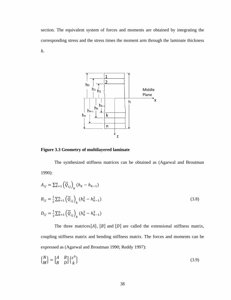
considering the equivalent system of forces and moments acting on the laminate cross
38
section. The equivalent system of forces and moments are obtained by integrating the
corresponding stress and the stress times the moment arm through the laminate thickness
.
Figure 3.3 Geometry of multilayered laminate
The synthesized stiffness matrices can be obtained as (Agarwal and Broutman
1990):
∑
∑ (3.8)
∑
The three matrices , and are called the extensional stiffness matrix,
coupling stiffness matrix and bending stiffness matrix. The forces and moments can be
expressed as (Agarwal and Broutman 1990; Reddy 1997):
(3.9)
39
where are the mid plane strains, are the plate curvatures,
are the resultant forces and are the resultant moments.
The extensional stiffness matrix relates the resultant forces to the mid-plane
strains, and the bending stiffness matrix relates the resultant moments to the plate
curvatures. The coupling matrix implies the coupling between bending and extension
of the plate, which means, the normal and shear forces acting at the mid-plane of the plate
result in not only the in-plane deformations, but also twisting and bending motions.
3.3 Governing Equations for the Vibration of Composite Laminate Plates
If the thickness of the laminate is very small compared to the dimension of the
plate, the classical laminated theory can be used to simplify the composite laminate plate
as a single-layer anisotropic plate. The material properties, orientation, thickness of each
plate can be taken into consideration in the stiffness matrices of the plate. The equations
of motion of the composite laminate plate are coupled and thus very difficult to solve for
the general solution of the displacements. However, at the high frequency, the following
convergence study shows that the coupling can be neglected.
In the following convergence study, we take the angle-ply plates as an example.
The equations of motion for free vibration of angle-ply plates with in-plane inertia
neglected can be expressed as (Whitney and Ashton 1987):
3 0
3 0
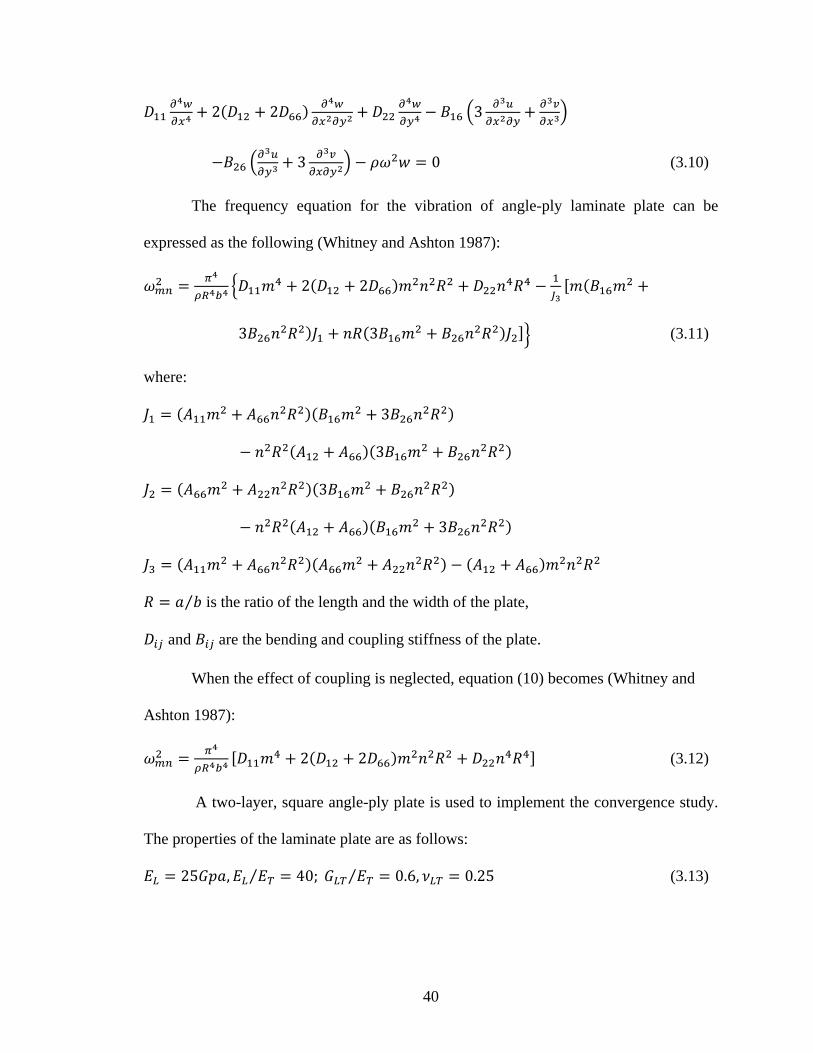
40
2 2 3
3 0 (3.10)
The frequency equation for the vibration of angle-ply laminate plate can be
expressed as the following (Whitney and Ashton 1987):
2 2
3 3 (3.11)
where:
3
3
3
3
⁄ is the ratio of the length and the width of the plate,
and are the bending and coupling stiffness of the plate.
When the effect of coupling is neglected, equation (10) becomes (Whitney and
Ashton 1987):
2 2 (3.12)
A two-layer, square angle-ply plate is used to implement the convergence study.
The properties of the laminate plate are as follows:
25 , 40; ⁄⁄ 0.6, 0.25 (3.13)

41
The exact frequency and the frequency with the coupling effect neglected are
calculated and plotted with respect to the increase of mode number for three different
angles of angle-ply laminate plates. The results are show in Figure 3.4.
(a) -30/30 angle-ply
(b) -45/45 angle-ply
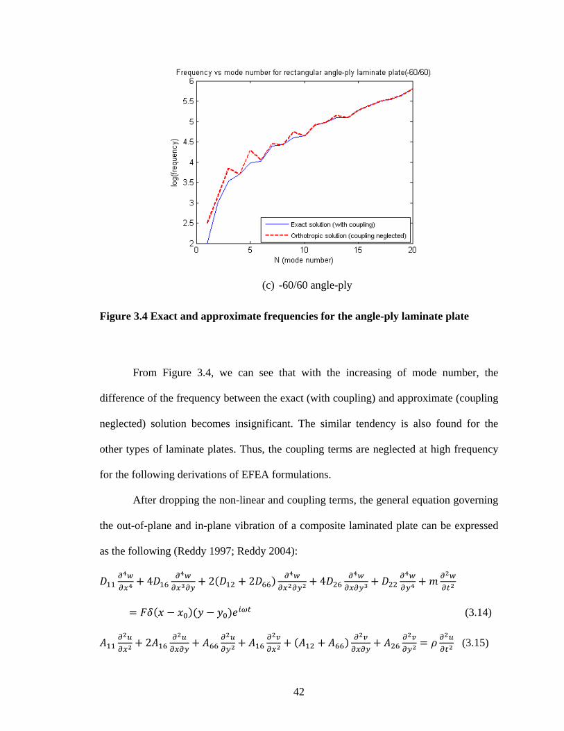
42
(c) -60/60 angle-ply
Figure 3.4 Exact and approximate frequencies for the angle-ply laminate plate
From Figure 3.4, we can see that with the increasing of mode number, the
difference of the frequency between the exact (with coupling) and approximate (coupling
neglected) solution becomes insignificant. The similar tendency is also found for the
other types of laminate plates. Thus, the coupling terms are neglected at high frequency
for the following derivations of EFEA formulations.
After dropping the non-linear and coupling terms, the general equation governing
the out-of-plane and in-plane vibration of a composite laminated plate can be expressed
as the following (Reddy 1997; Reddy 2004):
4 2 2 4
(3.14)
2 (3.15)

43
2 (3.16)
where are the bending stiffness, are the extensional stiffness, they can both be
obtained from the properties of each ply in the laminate, is the transverse displacement
of the plate, , are the and components of in-plane displacement in the middle plane
of the plate.
3.4 EFEA Development for the Flexural Waves in Composite Laminate Plates
3.4.1 Wave solution of displacement and the dispersion relation for flexural waves
The general form of the far-field solution of the equation of motion can be
obtained by considering the plane wave motion (Langley 1996):
, , (3.17)
where is the constant associated with the amplitude of propagating wave, and are
complex wave numbers associated with the damped frequency of oscillation in the x and
y directions.
1 , 1 (3.18)
where and are the real parts of wave numbers and .
Substituting the far-field solution to the equation of motion, we can get the
dispersion relation as follows (Langley 1996):
4 2 2 4 (3.19)
Let be the total wave number in the plate, and can be expressed as the
and components of as:

44
cos θ
sin θ (3.20)
where is the angle of wave propagation.
Substituting the above relationship into the dispersion relationship (3.19) yields
the expression of total wave number in terms of the wave propagation angle .
(3.21)
Because of the anisotropy of the composite laminate plate, the wave numbers in
the composite laminate plate depend on the direction of the wave propagation. In the
EFEA, the diffuse wave fields are assumed to exist in the plate. Thus, we need to take the
average of wave numbers by integrating it from 0 to 2 .
Integrate them over , and we can obtain the averaged wave numbers.
cos
sin (3.22)
At small damping, averaged complex wave numbers and can be expressed
approximated by the averaged wave numbers as (Bouthier and Bernhard 1992; Park,
Hong et al. 2003):
1
1 (3.23)

45
3.4.2 Derivation of time- and space- averaged energy density and intensities
Energy density is the amount of energy stored in a given system or region of
space per unit volume. Energy intensity is known as the amount of energy transported
past a given area of the medium per unit of time.
The total energy density is the sum of the kinetic and potential energy densities.
The time-averaged total energy density of the laminated plate can be expressed in terms
of the displacement as (Jones 1999):
2 4
4 4 (3.24)
The and components of the time-averaged intensity of a laminated plate can
be expressed by the forces and moments of the plate (Park, Hong et al. 2003):
(3.25)
(3.26)
For the laminate plate, the bending moments, twisting moments and the shear
forces can be expressed in terms of the displacement as the following (Whitney and
Ashton 1987):
2
2
2 (3.27)
2 3

46
2 3 (3.28)
Substituting the far-field displacement solution into the expressions and taking the
spatial average of the time-averaged energy density and intensities yield the time- and
space- averaged energy density and energy intensities (Fahy 1982):
⁄⁄ (3.29)
⁄⁄ (3.30)
⁄⁄ (3.31)
The time-averaged energy density and intensities are taken averaged over a half
wavelength for the above expressions. When the damping is small, all of the second order
and higher terms of the damping loss factor are neglected. After some manipulations, the
simplified expressions for the time- and space- averaged energy density and intensities
can be found as the following (see Appendix):
2 2 | | | |
| | | |
| | | | | | | |
(3.32)
2 | | | | | | | |
3 | | | | | | | |
(3.33)
2 | | | | | | | |
3 | | | | | | | |

47
(3.34)
where represents , , and represent the time- and
space-averaged energy density and energy intensities.
3.4.3 Derivation of EFEA differential equation and its variational statement
By observing the expressions of time- and space- averaged energy density and
intensities, we can find that the two parts of the and components of the time- and
space-averaged intensities are proportional to the first derivatives of two parts of the
time- and space-averaged energy density with respect to and :
, (3.35)
, (3.36)
where , , , are the four coefficients that can be expressed in terms of the
stiffness, frequency and wave numbers:
Considering the isotropic plate case, the bending stiffness can be expressed as:
, , , 0 (3.37)
48
where is the Young’s modulus and is the thickness of the plate.
Thus, for isotropic plate, the four coefficients can be simplified as:
, 0
where 2 is the group speed of the isotropic plate.
Therefore, for the isotropic plate, the following relationship can be obtained:
(3.38)
Equation (3.38) is the relationship between the time- and space- energy density
and intensities of isotropic plates; it appears same as equation (2.9). It is obtained as a
special case in our derivation and it appeared same as in (Bouthier and Bernhard 1992).
Considering a power balance at a steady state over a differential control volume
of the plate, the power balance equation can be written as (Bouthier and Bernhard 1992;
Bouthier and Bernhard 1995):
Π Π (3.39)
where the dissipated power and energy density can be expressed in the following
relationship (Cremer, Heckl et al. 1973):
Π (3.40)
Using the relationship between the dissipated power and energy density and the
relationship between energy density and energy intensity, the EFEA differential equation
with energy density as the primary variable can be obtained for the bending wave motion
of composite laminate plates:
Π Π (3.41)

49
In the EFEA differential equation, we made the assumption that the input power
splits into two parts. The subscript 1 corresponds to the stiffness
coefficients , , , , which correspond to the orthotropic plate, and the
subscripts 2 corresponds to the stiffness and .
In order to prove the above assumption of input power, we did the following
validation. A NASTRAN model is used to obtain the results in FEA model and a Fourier
expansion method is employed to obtain the results from EFEA formulation.
The analytic solution is obtained from the double Fourier series solution (Park,
Hong et al. 2003) to the out-of-plane equation of motion of a finite composite laminate
plate (3.14). It can be expresses as:
, , ∑ ∑ sin cos (3.42)
where is the coefficient of , mode of the displacement, , are the
dimension of the finite composite laminate plate. can be solved by substituting
equation (3.42) into equation (3.14).
(3.43)
The input power can be expressed in terms of the force and the velocity as
(Cremer, Heckl et al. 1973):
Π Re , , (3.44)
From equation (3.44), the input power for the composite laminate plate and the
corresponding orthotropic plate is calculated and the results are compared with the ones
obtained from very dense FEA model. Figure 3.5 presents the comparison of the input
power computed by the FEA model and the input power derived from the EFEA

50
formulation for the same laminate plate. Very good agreement is observed between the
two sets of results.
Figure 3.5 Input power comparison between FEA and analytic solutions
To develop a variational statement of the energy density differential equation
(3.41), we get the linear equation:
∑ ∑ 0 (3.45)
∑ ∑ 0 (3.46)
The terms are:
, Φ ,
,,
, · Γ
,, ,
, Φ Φ
, Φ Π ,
1000 1500 2000 2500 3000 3500 4000 4500 50000
0.5
1
1.5
2
2.5
3x 10⁻³
Frequency (Hz)
Inpu
t Pow
er
Πin1 (Analytic sulotion)Πin1 (FEA)Πin2 (Analytic sulotion)Πin2 (FEA)

51
A linear matrix equation can be developed as:
, ,,
, , 0 (3.47)
The subscript 1 corresponds to the stiffness coefficients , , , , which
correspond to the orthotropic plate, and the subscripts 2 corresponds to the stiffness
and . After getting the matrix formulation of the EFEA differential equation, we
are able to solve the differential equation numerically.
3.5 EFEA Development for the In-plane Waves in Composite Laminate Plates
3.5.1 Displacement solution the dispersion relationship for in-plane waves
The equations governing the in-plane vibration of the composite laminate plate
have been expressed in equations (3.15) and (3.16). Since the two displacement
components and are coupled with each other in the equations, it is difficult to obtain
the general displacement solution of the equations. However, the solution can be obtained
by using a displacement vector (Park, Hong et al. 2001):
, , , , , , (3.48)
where , , is a scalar quantity that represents the displacement potential which
corresponding to the dilational motion of the plate, , , is the a vector quantity that
represents the displacement potential which corresponds to the rotational motion of the
plate.
Substituting equation (3.48) into the plate’s in-plane equations of motion, we can
obtain the solution of the two displacement potentials and thus get the expression of
and from equation (3.48).
, , can be expressed as (Park, Hong et al. 2001):

52
, ,
(3.49)
where , are the and components of the complex longitudinal wavenumber .
The longitudinal wave component and of the in-plane displacements and
can be written as:
, , cos
(3.50)
, , sin
(3.51)
where , , , , cos ⁄ and sin
⁄ .
, , can be expressed as (Park, Hong et al. 2001):
, ,
(3.52)
where , are the and components of the complex in-plane shear wavenumber
.
Thus, the in-plane shear wave components and of the in-plane
displacements shear and can be written as:
, , sin
(3.53)
, , cos
(3.54)

53
where , , , , cos ⁄ and
sin ⁄ .
3.5.2 Derivation of time- and space- averaged energy density and intensities
The time-averaged total energy density of the in-plane vibration of thin composite
laminate plates can be written as:
(3.55)
The and components of the time-averaged in-plane vibration energy
intensities of the composite laminate plate can be expressed as:
(3.56)
(3.57)
Substituting equations (3.50) and (3.51) into equations (3.55)-(3.57), and taking
the spatial average of the time-averaged energy density and intensities over a half
wavelength yield the time- and space- averaged energy density and energy intensities for
the longitudinal motion of the plate.

54
2 | |
| | | | | | 2 | |
| | | | | | (3.58)
| | | | | | | |
2 | | | | | | | | (3.59)
| | | | | | | |
2 | | | | | | | | (3.60)
Similarly, the time- and space- averaged energy density and energy intensities for
the in-plane shear waves can be derived by substituting equations (3.53) and (3.54) into
equations (3.55)-(3.57):
2 2 | |
| | | | | | 2 | |
| | | | | | (3.61)
| | | | | |
| | 2 | | | | | |
| | (3.62)
| | | | | |
| | 2 | | | | | |
| | (3.63)
where represents , , and represent the time- and
space-averaged energy density and energy intensities.

55
3.5.3 Derivation of EFEA differential equations for in-plane motions
Similar to section 3.4.3, we can find that for both longitudinal and in-plane shear
wave motions, the two parts of the and components of the time- and space-averaged
intensities are proportional to the first derivatives of two parts of the time- and space-
averaged energy density with respect to and . The relationship similar to equations
(3.35) and (3.36) can be found for the longitudinal and in-plane shear wave motions
respectively.
For the longitudinal wave motion:
, (3.64)
, (3.65)
where , , , are the four coefficients that can be expressed in terms of the
stiffness, frequency and wave numbers:
For the in-plane shear wave motion:
, (3.66)
, (3.67)
where , , , can be expressed as follows:

56
Using the relationship between the dissipated power and energy density and the
relationship between energy density and energy intensity, the EFEA differential equation
with energy density as the primary variable can be obtained for the in-plane wave motion
of composite laminate plates.
For longitudinal wave motion:
Π Π (3.68)
For in-plane shear wave motion:
Π Π (3.69)
3.6 Numerical Examples and Validation
In order to demonstrate the validity of the new EFEA formulation in composite
laminate plates, the results from very dense FEA models are used to compare the results
from the EFEA model of two types of laminate plates. In both examples, the bending
motion of the plate is studied.

57
3.6.1 Two-layer cross-ply laminate plate
In this example, the vibration of a two-layer cross-ply composite laminate plate
with several excitations on the plate is analyzed using FEA and EFEA models
respectively at several different frequencies. The plate is a 1m×1m square cross-ply
(0/90) plate with two layers of equal thickness. Layers with the following engineering
constants are used:
25 , 40 , 0.6 , 0.25 (3.70)
Figure 3.6 Configuration of two-layer cross-ply laminate plate
The thickness of each layer is 0.0025m. The bending stiffness matrix can be
obtained from the properties, thickness and orientation of the two layers and they are
expressed in the matrix.
134.0 1.63 01.63 134.0 0
0 0 3.91· (3.71)
Figure 3.7 presents the laminate plate models in FEA and EFEA respectively. To
capture the response of the plate at high frequencies, the conventional FEA model has
10,000 elements. The EFEA model has only 100 elements.
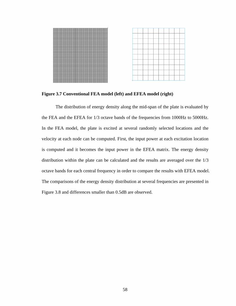
58
Figure 3.7 Conventional FEA model (left) and EFEA model (right)
The distribution of energy density along the mid-span of the plate is evaluated by
the FEA and the EFEA for 1/3 octave bands of the frequencies from 1000Hz to 5000Hz.
In the FEA model, the plate is excited at several randomly selected locations and the
velocity at each node can be computed. First, the input power at each excitation location
is computed and it becomes the input power in the EFEA matrix. The energy density
distribution within the plate can be calculated and the results are averaged over the 1/3
octave bands for each central frequency in order to compare the results with EFEA model.
The comparisons of the energy density distribution at several frequencies are presented in
Figure 3.8 and differences smaller than 0.5dB are observed.
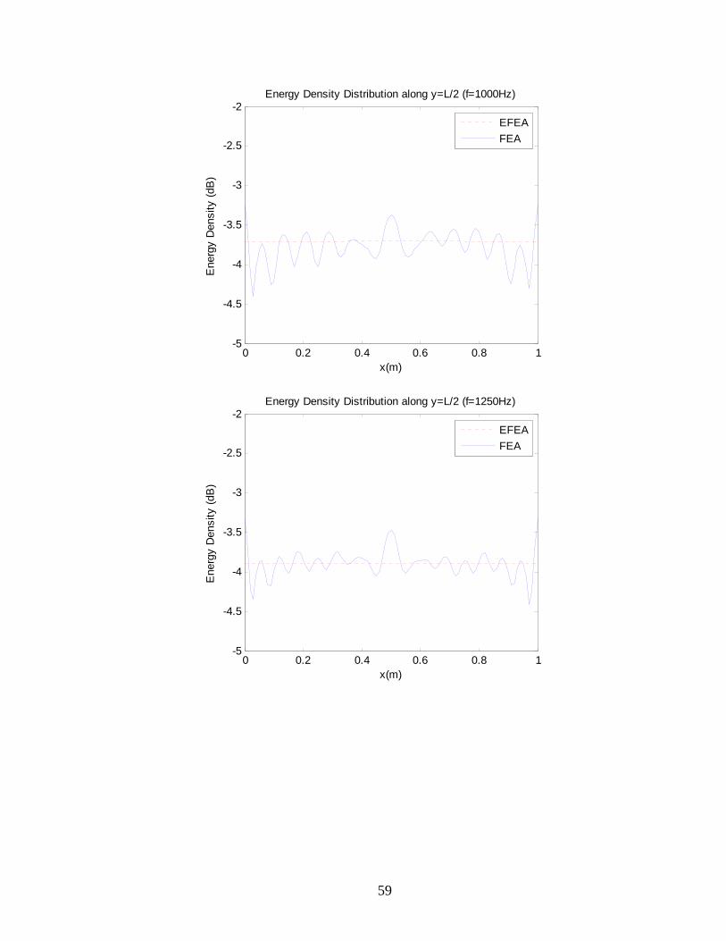
59
0 0.2 0.4 0.6 0.8 1-5
-4.5
-4
-3.5
-3
-2.5
-2Energy Density Distribution along y=L/2 (f=1000Hz)
x(m)
Ene
rgy
Den
sity
(dB
)
EFEAFEA
0 0.2 0.4 0.6 0.8 1-5
-4.5
-4
-3.5
-3
-2.5
-2Energy Density Distribution along y=L/2 (f=1250Hz)
x(m)
Ene
rgy
Den
sity
(dB
)
EFEAFEA

60
0 0.2 0.4 0.6 0.8 1-5.5
-5
-4.5
-4
-3.5
-3
-2.5
-2Energy Density Distribution along y=L/2 (f=1600Hz)
x(m)
Ene
rgy
Den
sity
(dB
)
EFEAFEA
0 0.2 0.4 0.6 0.8 1-5.5
-5
-4.5
-4
-3.5
-3
-2.5Energy Density Distribution along y=L/2 (f=2000Hz)
x(m)
Ene
rgy
Den
sity
(dB
)
EFEAFEA

61
0 0.2 0.4 0.6 0.8 1-5.5
-5
-4.5
-4
-3.5
-3
-2.5Energy Density Distribution along y=L/2 (f=2500Hz)
x(m)
Ene
rgy
Den
sity
(dB
)
EFEAFEA
0 0.2 0.4 0.6 0.8 1-5.5
-5
-4.5
-4
-3.5
-3
-2.5Energy Density Distribution along y=L/2 (f=3150Hz)
x(m)
Ene
rgy
Den
sity
(dB
)
EFEAFEA

62
Figure 3.8 Distribution of energy density along the mid-span of the cross-ply
laminate plate computed by the dense FEA and EFEA models at 1000Hz-5000Hz 1/3
octave bands
0 0.2 0.4 0.6 0.8 1-5.5
-5
-4.5
-4
-3.5
-3
-2.5Energy Density Distribution along y=L/2 (f=4000Hz)
x(m)
Ene
rgy
Den
sity
(dB
)
EFEAFEA
0 0.2 0.4 0.6 0.8 1
-5.5
-5
-4.5
-4
-3.5
-3
Energy Density Distribution along y=L/2 (f=5000Hz)
x(m)
Ene
rgy
Den
sity
(dB
)
EFEAFEA

63
3.6.2 Two-layer general laminate plate
In this part, the example of a more general composite laminate plate is calculated
in conventional EFA and EFEA models. The plate is a 1m×1m square laminated plate
with two layers of equal thickness. The two layers are at 0 and 45 degree orientation.
Layers with the following engineering constants are used:
20 , 2 , 0.7 , 0.35 (3.72)
The configuration of the laminate is illustrated in the following Figure 3.9.
Figure 3.9 Configuration of composite laminate plate
The thickness of each layer is 0.0025m. The bending stiffness matrix can be
calculated as:
140.0 30.9 23.730.9 45.0 23.723.7 23.7 30.8
(3.73)
The comparisons of the energy density distribution at mid-span of the plate at
several frequencies are presented in Figure 3.10. Similar to the example of cross-ply
laminate plate, very good agreement can be observed from the comparison between
EFEA and FEA results. EFEA captures the energy distribution level in the plate well
while using a significantly smaller number of elements.
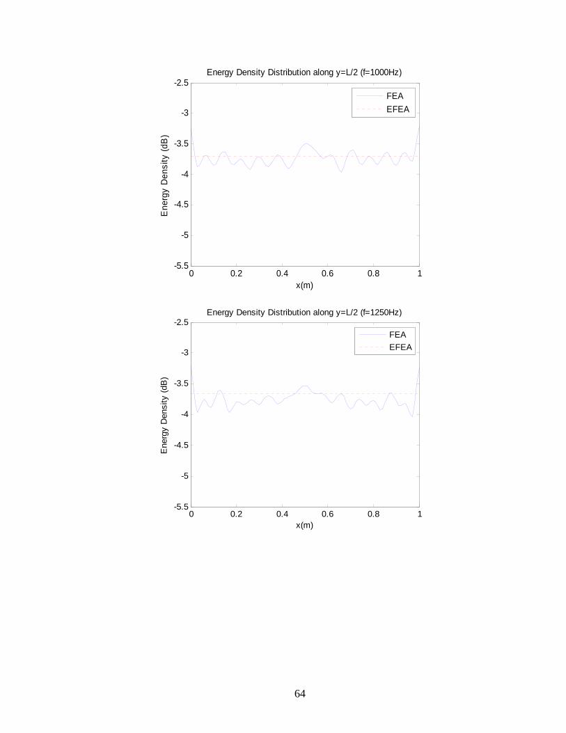
64
0 0.2 0.4 0.6 0.8 1-5.5
-5
-4.5
-4
-3.5
-3
-2.5Energy Density Distribution along y=L/2 (f=1000Hz)
x(m)
Ene
rgy
Den
sity
(dB
)
FEAEFEA
0 0.2 0.4 0.6 0.8 1-5.5
-5
-4.5
-4
-3.5
-3
-2.5Energy Density Distribution along y=L/2 (f=1250Hz)
x(m)
Ene
rgy
Den
sity
(dB
)
FEAEFEA

65
0 0.2 0.4 0.6 0.8 1-5.5
-5
-4.5
-4
-3.5
-3
-2.5Energy Density Distribution along y=L/2 (f=1600Hz)
x(m)
Ene
rgy
Den
sity
(dB
)
FEAEFEA
0 0.2 0.4 0.6 0.8 1-5.5
-5
-4.5
-4
-3.5
-3
-2.5Energy Density Distribution along y=L/2 (f=2000Hz)
x(m)
Ene
rgy
Den
sity
(dB
)
FEAEFEA

66
0 0.2 0.4 0.6 0.8 1-5.5
-5
-4.5
-4
-3.5
-3
-2.5Energy Density Distribution along y=L/2 (f=2500Hz)
x(m)
Ene
rgy
Den
sity
(dB
)
FEAEFEA
0 0.2 0.4 0.6 0.8 1-5.5
-5
-4.5
-4
-3.5
-3
-2.5Energy Density Distribution along y=L/2 (f=3150Hz)
x(m)
Ene
rgy
Den
sity
(dB
)
FEAEFEA
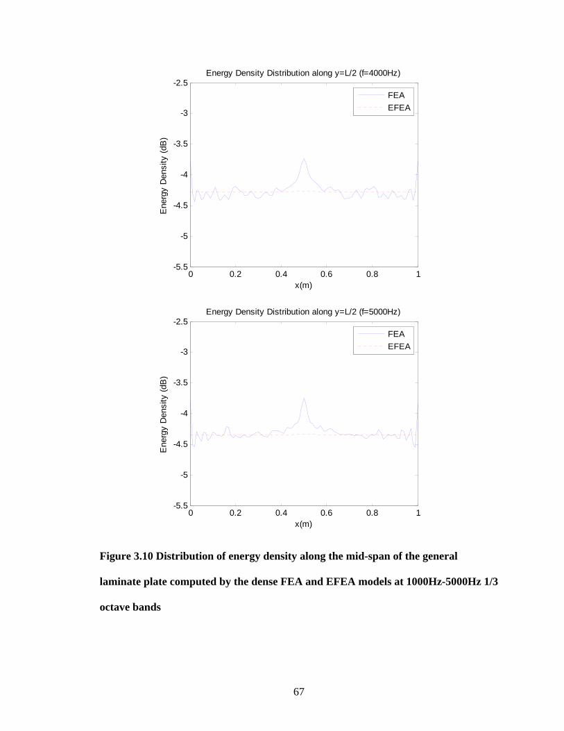
67
Figure 3.10 Distribution of energy density along the mid-span of the general
laminate plate computed by the dense FEA and EFEA models at 1000Hz-5000Hz 1/3
octave bands
0 0.2 0.4 0.6 0.8 1-5.5
-5
-4.5
-4
-3.5
-3
-2.5Energy Density Distribution along y=L/2 (f=4000Hz)
x(m)
Ene
rgy
Den
sity
(dB
)
FEAEFEA
0 0.2 0.4 0.6 0.8 1-5.5
-5
-4.5
-4
-3.5
-3
-2.5Energy Density Distribution along y=L/2 (f=5000Hz)
x(m)
Ene
rgy
Den
sity
(dB
)
FEAEFEA

68
3.7 An Alternative Method to Derive the EFEA Differential Equation for Composite
Laminate Plates
3.7.1Group velocity for composite laminate plates
From the classical laminate theory, composite laminate plate can be considered as
an anisotropic plate. The wavenumber has angle dependence in anisotropic media
(Bosmans, Mees et al. 1996; Bosmans, Vermeir et al. 2002). The energy distribution and
the direction of energy flow in anisotropic media are affected by the angle dependence of
the wavenumber. Poynting vector is used in describing the energy flow in anisotropic
media (Auld 1990). This vector, which is parallel to the heading of the group velocity, is
orientated normal to the curve obtained by plotting the wavenumber as a function of the
wave heading. Thus, the heading of group velocity is different to the heading of wave
propagation, except for some values. Figure 3.11 gives an illustration of this phenomenon.
Figure 3.11 Wavenumber as a function of wave heading in the wavenumber plane

69
The component of group velocity is expressed as , the component along the
heading of wave propagation is expressed as . The angle between and is the
heading of group velocity .
The following relations exist for the wave propagation:
(3.74)
(3.75)
Now let’s derive the group velocity for bending waves in composite laminate
plates. For composite laminate plate, the bending wavenumber is expressed in equation
(3.21) (Bosmans, Vermeir et al. 2002).
(3.76)
The normal vector of the wavenumber curve can be expressed as:
tan ⁄⁄
⁄⁄ (3.77)
where can be obtained from equation (3.21).
From Figure 3.11, the following relationship between and can be
obtained:
(3.78)
The group velocity corresponding to the bending wave can be calculated from
equation (3.78). The group velocity of the in-plane waves can also be calculated
following the similar procedure.

70
3.7.2 Equivalent homogenized isotropic material for composite laminate plates
From Chapter 2, we know that the EFEA differential equation for isotropic
material can be expressed as (Bouthier and Bernhard 1992):
Π (3.79)
2 (3.80)
The property of the material is taken into consideration in the group velocity of
the material. For the composite laminate plate, it is also possible to come up with a
similar EFEA differential equation by using the averaged group velocity . As described
previously, the group velocity for composite laminate plate is a function of wave
propagation angle . The averaged group velocity removed the dependency to by
taking the average of from 0 to 2 .
(3.81)
Using the averaged group velocity, we can express the EFEA differential equation
for composite laminate plate as:
Π (3.82)
At element level, the EFEA differential equation can be expressed as:
(3.83)
where is the vector of nodal values for the time and space averaged energy density,
is the system matrix for each element, is the excitation vector, it represents the
energy input at each node, is the power flow across the element boundary.

71
From the averaged group velocity for composite laminate plate, we can find its
equivalent isotropic material property using equation (3.80).
(3.84)
3.7.3 Validation of alternative approach
The two-layer general composite laminate plate used in 3.6.2 is used to implement
the validation. In the calculation, the energy density distribution of plate is calculated
using EFEA differential equation derived for both the composite laminate plate and the
equivalent isotropic plate. The results for the frequency 1000 Hz and 5000 Hz are plotted
in Figure 3.12. In both plots, good correlation is observed between these two methods.
(a) f =1000 Hz
0 0.2 0.4 0.6 0.8 1-3.7075
-3.707
-3.7065
-3.706
-3.7055
-3.705
x(m)
Ene
rgy
Den
sity
(dB
)
Composite laminateEquivalent isotropic

72
(b) f =5000 Hz
Figure 3.12 Energy density distribution comparison between composite laminate
plate and its equivalent isotropic plate
0 0.2 0.4 0.6 0.8 1-4.4059
-4.4059
-4.4058
-4.4058
-4.4057
-4.4056
-4.4056
-4.4055
-4.4055
x(m)
Ene
rgy
Den
sity
(dB
)
Composite laminateEquivalent isotropic

73
Chapter 4
POWER TRANMISSION THROUGH COUPLED ORTHOTROPIC PLATES
4.1 Introduction
In order to analyze the power transmitted from the excitation location to the other
components within the structure at high frequency, it is necessary to calculate the
vibrational energy transmission at the plate junctions. The power transmission
coefficients can be utilized to form the joint matrix at the structural junctions, where the
energy density value is discontinuous. It is then possible to assemble the global system of
matrix of EFEA differential equation and solve for the energy density throughout the
entire system.
Approaches to calculate the power transmission coefficients include the methods
for semi-infinite plates and finite-sized plates, but both methods are based on the proper
formulation of the continuity and equilibrium conditions at the junction. In the past, this
problem has been solved for thin (Langley and Heron 1990) and thick plates (Mccollum
and Cuschieri 1990), for plate junction with beams (Langley and Heron 1990), junctions
with elastic interlayer (Wohle, Beckmann et al. 1981; Mees and Vermeir 1993), junction
of curved panels (Langley 1994).
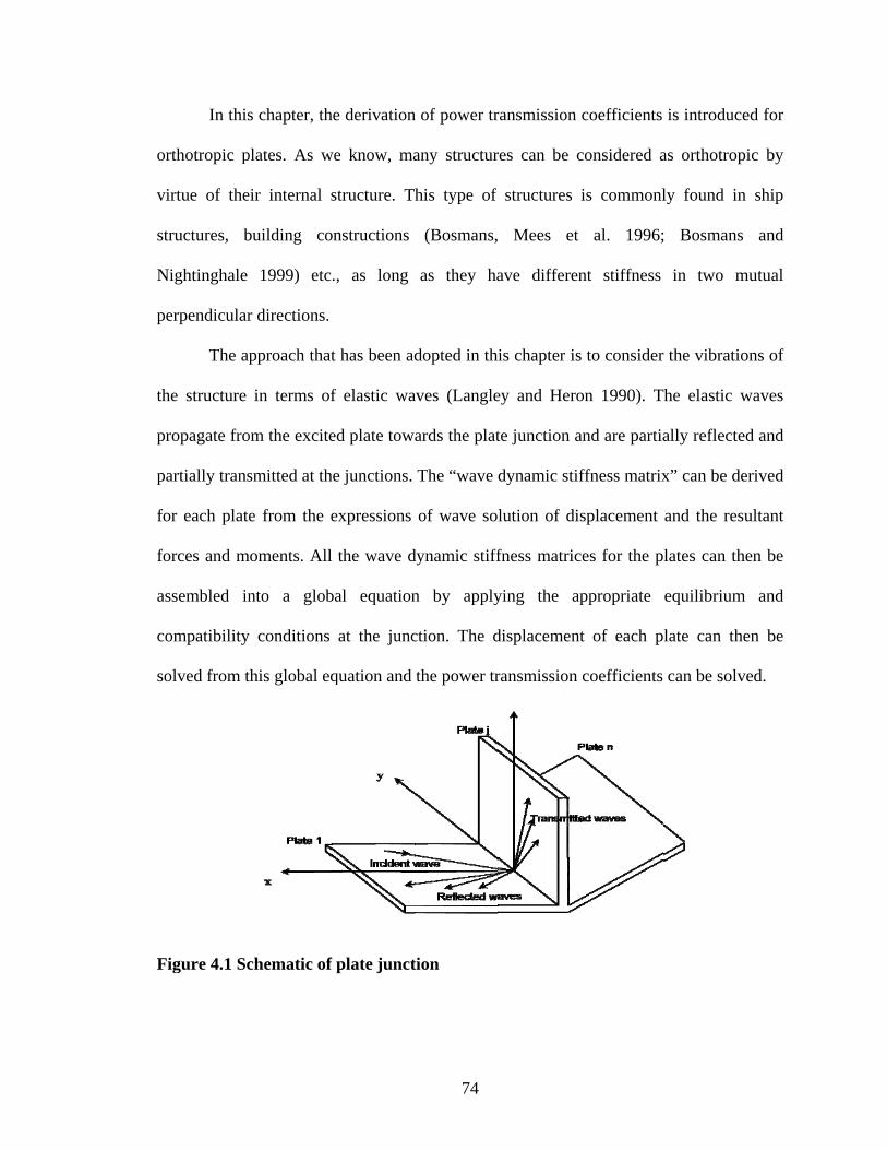
or
v
st
N
p
th
pr
p
fo
fo
as
co
so
F
In this
rthotropic p
irtue of the
tructures, b
Nightinghale
erpendicular
The ap
he structure
ropagate fro
artially trans
or each plate
orces and m
ssembled in
ompatibility
olved from t
Figure 4.1 Sc
s chapter, th
plates. As w
eir internal s
building co
1999) etc
r directions.
pproach that
in terms of
om the excite
smitted at th
e from the e
moments. All
nto a glob
y conditions
this global eq
chematic of
he derivation
we know, ma
structure. Th
onstructions
., as long
t has been ad
f elastic wa
ed plate tow
he junctions.
expressions
the wave d
bal equation
at the junc
quation and
f plate junct
74
n of power tr
any structur
his type of
(Bosmans,
as they ha
dopted in th
aves (Langle
ards the plat
The “wave
of wave so
dynamic stiff
n by apply
ction. The d
the power tr
tion
ransmission
res can be c
f structures
Mees et
ave differen
is chapter is
ey and Hero
te junction a
dynamic stif
lution of dis
fness matric
ying the ap
displacement
ransmission
coefficients
considered a
is commonl
al. 1996;
nt stiffness
s to consider
on 1990). T
and are partia
ffness matrix
splacement
ces for the p
ppropriate
t of each p
coefficients
is introduce
as orthotropi
ly found in
; Bosmans
in two m
r the vibratio
he elastic w
ally reflected
x” can be de
and the resu
lates can the
equilibrium
late can the
can be solve
ed for
ic by
ship
and
mutual
ons of
waves
d and
erived
ultant
en be
and
en be
ed.

75
Figure 4.1 gives a schematic plot of a junction that consists of an arbitrary number
of coupled plates. There are three types of waves involved in the plate junction problem:
bending, longitudinal and shear waves.
This chapter is organized as follows. First, the equations of motion that govern the
wave propagation in orthotropic plates are presented. The solutions for the equations are
introduced, including the derivation of in-plane wavenumbers for orthotropic plates.
Second, the wave dynamic stiffness matrix is derived, the global equation is assembled
and the power transmission coefficients are solved. Third, the joint matrix is formed in
terms of the power transmission coefficients and the global matrix of EFEA differential
equation is form to solve for the energy density distribution within the structure. Finally,
numerical examples are presented using the L-junction of two orthotropic plates with
different orientations and the results obtained from EFEA formulation are compared with
the results from very dense FEA model.
4.2 Derivation of Power Transmission Coefficients for Orthotropic Plate Junction
4.2.1 Governing equations
The deformation of each plate is defined with respect to the local coordinate
system, which has the x-axis along the connection edge, as shown in Figure 4.2. The
equations of motion that govern the deflections of the th plate can be written in the form
(Whitney and Ashton 1987) :
2 2 0 (4.1)
0 (4.2)

76
0 (4.3)
where , etc. are the coefficients of bending and extensional stiffness matrices of
th plate.
Figure 4.2 Coordinate system, displacements, forces and moments for plate j
The relationship between the displacements and the traction that act at the
connected edge of the plate can be expressed as follows (Ashton and Whitney 1970).
(4.4)
2 (4.5)
(4.6)
(4.7)
The tractions that act on the common edge of the plates are evaluated at 0.
The forces and moments per unit length that are applied to the junction by the
semi-infinite plates can be expressed as (Langley and Heron 1990):
∑ (4.8)
77
where represents the tractions on the connected edge of plate , and
the transformation matrix is given by (Langley and Heron 1990):
1 00 cos
0 0sin 0
0 sin0 0
cos 0 0 1
(4.9)
where is the angle of the local coordinate in plate with respect to the global
coordinate system.
The compatibility conditions between the common junction displacement , and
the edge displacement of plate , require that
(4.10)
where , , and , , are the displacements
of the junction in x, y, z directions respectively, is the rotation of the junction with
respect to the x axis, , , , are the corresponding displacements and
moments for plate .
4.2.2 Derivation of in-plane wavenumbers for orthotropic plates
The in-plane equations of motion for orthotropic plates can be expressed in
equation (4.2) and (4.3). In the case of isotropic materials, these two equations predict
two modes of propagation – longitudinal and shear modes. However, in the case of
orthotropic material, because of the anisotropy, the modes are not pure longitudinal and
pure shear except when they are propagating along directions of material symmetry. In
general, these two modes are referred as quasi-longitudinal and quasi-shear modes
(Prosser 1991).

78
The dispersion relationship for the orthotropic case is much more complicated
than the isotropic case. Because of the anisotropy, the velocity of the mode is dependent
on the direction of wave propagation. The dispersion relationship will again be obtained
by assuming a plane wave form of the displacement and substituting into the equations of
motion. The in-plane displacements are given by (Prosser 1991):
cos sin (4.11)
cos sin (4.12)
where and are the amplitudes of the two in-plane motions, is the in-plane
wavenumber, is the angle of wave propagation.
Substituting these displacements into the equations of motion yields the following
relationship:
cos sin cos sincos sin cos sin
0
(4.13)
The non-trivial solution for this equation will be obtained only when the
determinant of the matrix is equal to zero. Setting the determinant equal to zero will yield
a quadratic equation of . The two solutions of wavenumber correspond to the quasi-
longitudinal and quasi-shear modes respectively. Generally, the quasi-longitudinal mode
is faster and thus corresponds to the smaller root.
For the wave propagation along the axis or the 0 degree direction of the
laminate, we have cos 1, sin 0. Thus, equation (4.13) becomes:
00
0 (4.14)
The non-trivial solution requires:
79
00
0 (4.15)
where ⁄ is the phase velocity.
The two solutions can be solved:
(4.16)
(4.17)
In this case, 10 or 0
1 , which correspond to a pure longitudinal wave
mode or a pure shear wave mode.
4.2.3 Derivation of dynamic stiffness matrix
The wave dynamic stiffness matrix is derived by considering a plane wave
propagating through one of the semi-infinite plates towards the plate junctions and being
partly reflected to the plate and partly transmitted to other plates.
Assume the incident wave have a form of exp , the Snell’s
law requires that the response in all the plates must have the same dependency
exp , the dependency will be determined from the plate equation of
motion.
Assume the out-of-plane displacement of plate has the form of exp
, can be expressed as:
(4.18)
where is the bending wavenumber, it
depends on the direction of wave propagation .

80
If , equation (4.18) will have four real roots, in this case, only the two
negative roots are physically significant because the response must decay as ∞. In
the case that , equation (4.18) will have two real roots and two imaginary roots. In
this case, only the negative real root and the negative imaginary root should be selected,
because the response must either decay as ∞ or propagate away from the junction
(Langley and Heron 1990). After selecting the right component of wavenumber , the
out-of-plane response of the plate can be written in the form:
∑ exp (4.19)
where and are the two valid roots from equation (4.18), and are the
complex amplitudes associated with two roots.
The rotation can be expressed as:
(4.20)
From equation (4.19) and (4.20), the displacement and rotation at the edge of the
plate can be evaluated at 0, they can be expressed in terms of , and
(Langley and Heron 1990):
1 1 exp (4.21)
From equations (4.4) and (4.5) and equation (4.19), the edge tractions and
can be expressed in terms of and as:
4 4
exp (4.22)
From equation (4.21), we can express and in terms of and as:

81
1 1 exp (4.23)
Eliminate and from equation (4.22) using equation (4.23), we can get the
following relationship between the edge displacements , and the edge tractions
and :
4
(4.24)
Similar procedure can be used to determine the in-plane behavior of the plate. In
order to simplify the derivation calculation, we assume the in-plane motions in the
following expressions instead of equations (4.11) and (4.12) (Bosmans, Mees et al.
1996):
(4.25)
(4.26)
where is the ratio between the amplitudes of the two displacements.
Substituting equations (4.25) and (4.26) into the in-plane equations of motion
(4.2) and (4.3), we can get the following expression:
1 00 (4.27)
Take the determinant equal to zero yield a polynomial equation of . Among the
four roots of only the real and negative or imaginary and negative roots are selected.
They are the corresponding components of longitudinal and shear wavesnumbers
respectively. Associated with each root is a mode shape which governs the relationship
82
between the two in-plane displacements. The two mode shapes can be obtained as 1
and 1 .
Thus, the in-plane response can be written in the form:
1 e 1 e exp (4.28)
where and are the complex amplitudes of the associated complementary functions.
Thus, the edge displacements and can be also expressed in terms of and as:
1 1 exp (4.29)
Similarly, we can express the edge tractions and in terms of and as:
(4.30)
Eliminate and from equation (4.30) using equation (4.29), we can get the
following relationship between the edge displacements , and the edge
tractions and :
(4.31)
Equations (4.24) and (4.31) can be combined to produce a relationship between
the complete set of edge displacements and tractions of the form:
(4.32)
where and
(4.33)

83
where the entries of matrix have been derived and can be found from equation (4.24)
and (4.31).
22 1 2 12
22
212 4 66 1 2 22 2
31
3
22 1 2 2 12
12 2 1
22 12
22
0
This matrix is called the dynamic stiffness matrix of the semi-infinite plate .
If the incident wave is carried by plate , then equation (4.32) needs to be
modified as (Langley and Heron 1990):
(4.34)
(4.35)
where and are the edge displacements and tractions caused by the incident wave.
The vectors can be expressed as the followings for the incident wave as
bending wave, longitudinal wave and shear wave respectively (Langley and Heron 1990).
For bending incident wave:

84
00 (4.36)
where , .
For longitudinal incident wave:
00
(4.37)
For shear incident wave:
00
(4.38)
The vector can be expressed as product of the dynamic stiffness caused by the
incident wave and . is calculated by using the same coefficient in the matrix
but with the opposite sign of , which corresponds to the incident wave instead of the
reflected wave.
4.2.4 Assembly of the complete equations and the calculation of transmission coefficients
Equation (4.8) gives the forces and moments per unit length that are acted on the
junction by all the semi-infinite plates. With equation (4.32) and equation (4.10), we
can get the following equation (Langley and Heron 1990):
∑ (4.39)
where is the plate that carries the incident wave.
Equation (4.39) can be solved to get the displacement at the junction; it is also
the common displacements of at the plate edge of all the semi-infinite plates. Equation
(4.10) can be used to obtain the displacement of each plate. Equations (4.21) and (4.29)

85
can then be used to calculate the corresponding wave amplitudes of bending, shear and
longitudinal waves.
The power associated with each wave can be calculated using the corresponding
wave amplitudes. The power transmission coefficients associated with each of the
generated waves can then be calculated as the ratio of the transmitted power to the total
incident power on the junction. The transmission coefficients for the junction can be
written in the form , , where , , and represent the incident plate, wave type,
frequency and the heading of the incident wave, and represent the carrier plate and
wave type of the generated wave. , is also often referred as , as the
reflection coefficients for .
From the law of conservation of energy, we can prove that the transmission and
reflection coefficient sum equal to unity, since the total power that is incident on the
junction must equal the total power which is carried away by the generated waves.
∑ ∑ , 1 (4.40)
During the derivation of power transmission coefficients, the bending and in-
plane wavenumbers are dependent on the angle of incident wave. Thus, the above
expression of transmission coefficients is also the function of the incident angle . The
averaged coefficient values are selected for the analysis. The averaged power
transmission coefficient can be obtained by integration as:
, sin (4.41)

86
4.3 Derivation of Joint Matrix
4.3.1 Power flow relationship of two systems through a lossless joint
In this section the, some background of forming the joint matrix between two
systems are introduced first. The joint matrix is derived by considering the energy flow
between two structures (Bitsie and Bernhard 1996). The conservation of energy flow
requires the net outward energy flow for a single wave across the boundary of one system
must be equal and opposite to the energy flow across the boundary of the other system.
The conservation of energy flow relationship can be expressed as:
· · · 0 (4.42)
where subscripts 1 and 2 denote the individual subsystems 1 and 2.
Figure 4.3 gives a schematic plot of energy flow between two subsystems through
a lossless joint for a single wave. The surface normal defines the positive direction of
power flow out of the lossless joint.
Figure 4.3 Schematic plot of energy flow between two subsystems for a single wave
The expression of energy flow across the lossless joint are (Bitsie and Bernhard
1996):

87
· · · (4.43)
· · · (4.44)
where and are incident energy flows in subsystems 1 and 2, and
are the scattered energy flows from the discontinuity in each subsystem. The energy flow
is denoted as positive when it flows out of the system.
The scattered energy flows can be expressed in terms of the incidents waves,
power transmission and power reflection coefficients:
| | | | | | (4.45)
| | | | | | (4.46)
where and are the reflection and transmission coefficients in subsystem due to the
incident wave in subsystem .
After substituting equations (4.45) and (4.46) into equations (4.43) and (4.44), we
find the following relationship between the energy flow and the incident energy
intensities:
· ·
11
| |
| | | |
| | (4.47)
The energy superposition relationship for energy field requires:
(4.48)
(4.49)
Integrate equations (4.48) and (4.49) and using the relationship | |, we can
get the following expressions:
| | | | (4.50)

88
| | | | (4.51)
Substituting equations (4.45) and (4.46) into equations (4.50) and (4.51) yields the
following expressions (Bitsie and Bernhard 1996):
1
1| |
| | | |
| | (4.52)
Combining equations (4.47) and (4.52) yield the relationship between energy
density to the intensities:
· ·
(4.53)
where is the joint matrix.
For the two subsystems connected, the joint matrix can be expressed as:
11
11
(4.54)
Conservation of energy requires:
1 (4.55)
1 (4.56)
Thus the joint matrix for two subsystems can be simplified as (Bitsie and
Bernhard 1996):
(4.57)

89
4.3.2 Joint matrix for two coupled plates
The derivation of joint matrix for coupled plates has the similar formula as
described in equation (4.54). First, the transmission coefficients matrix between two
plates can be expressed as in a matrix as:
, ,, ,
, ,, ,
, ,, ,
, ,, ,
, ,, ,
, ,, ,
, ,, ,
, ,, ,
, ,, ,
(4.58)
where , represents the (=1, 2, 3, where 1 indicates the bending wave, 2 indicates the
in-plane longitudinal wave, and 3 indicates the in-plane shear wave) wave type power
reflection coefficient in plate (=1,2) due to the incident wave type in plate , ,
represents the wave type power transmission coefficient in plate due to the incident
wave type in plate .
Let be the unit matrix, and
(4.59)
(4.60)
Similar to equation (4.54), the matrix can be expressed as:
· (4.61)
Then the joint matrix can be calculated by:
(4.62)

90
where is calculated by the integral along the joint line in the form same as that for
a consistent mass matrix.
4.4 Assembly of Global Matrix for Coupled Orthotropic Plates
From Chapter 2, the matrix expression of EFEA differential equation at the
element level can be expressed as:
(4.63)
where is the vector of nodal values for the time and space averaged energy density,
is the system matrix for each element, is the excitation vector, it represents the
energy input at each node, is the power flow across the element boundary.
The power flow can be expressed in terms of energy density and power
transmission coefficients.
(4.64)
where and 1 represents the two nodes of the element at the joint, and 1
represents the two nodes of the element at the joint, the joint matrices define the
power transfer across elements at the joints and is expressed in equation (4.62).
The final assembled system of EFEA equations can be expressed as:
(4.65)
where and are the element matrix for the and element, and are
the vectors containing all the nodal degrees of freedom for elements and .

91
4.5 Numerical Examples and Validation
In this section, numerical calculation will be presented for the case of L-junction
of two identical orthotropic plates connected with different orientations. The EFEA
results are validated by comparing with results obtained from conventional FEA models.
The dimensions and the material properties of the orthotropic plates can be
expressed as:
0.01 , 1 , 1
40.0 , 20.0 , 11.54 , 0.3 (4.66)
2500 ⁄ , 0.01
Four cases of the L-junction are considered in the calculation based on the
different orientations of the two orthotropic plates. Figure 4.4 gives the explanation of the
four different cases of the L-junction. The arrows on each plate indicate the stiffest
principal material direction. In cases 1 and 4, the two plates have identical orientations
while in cases 2 and 3; the two plates have different orientations.
Figure 4.4 Four different orientations for two orthotropic plate L-junctions
The calculation in conventional FEA is implemented using NASTRAN finite
element program. Plate 1 is given excitation at three randomly selected positions and the

92
velocities of both plates are calculated from dynamic analysis. The bending wave energy
density of two plates can then be calculated and compared with the energy density
calculated using EFEA formulation.
First, the transmission loss for bending wave is calculated using the procedure
stated in section 4.2. Transmission loss is calculated as (Bosmans, Mees et al. 1996):
10log (4.67)
where is the averaged bending transmission coefficient from plate 1 to plate 2, it is
obtained by integrating the power transmission coefficient over all the angles of
incidence .
The transmission loss for the four different orientations of L-junction has been
calculated and plotted in Figure 4.5. From the plot we can see that the transmission loss
for the similar orientation (case 1 and case 4) is smaller than the transmission loss of the
dissimilar orientation (case 2 and case 3). It can also be observed from the plot that the
transmission loss of the four cases lie within a range of 1 dB, which means that the model
for the semi-infinite plate is not very sensitive to the Young’s modulus of the plates.
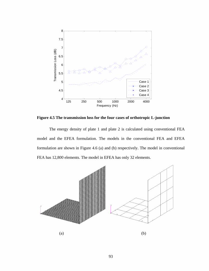
93
Figure 4.5 The transmission loss for the four cases of orthotropic L-junction
The energy density of plate 1 and plate 2 is calculated using conventional FEA
model and the EFEA formulation. The models in the conventional FEA and EFEA
formulation are shown in Figure 4.6 (a) and (b) respectively. The model in conventional
FEA has 12,800 elements. The model in EFEA has only 32 elements.
(a) (b)
125 250 500 1000 2000 40004
4.5
5
5.5
6
6.5
7
7.5
8
Frequency (Hz)
Tran
smis
sion
Los
s (d
B)
Case 1Case 2Case 3Case 4
94
Figure 4.6 The models of orthotropic L-junction in conventional FEA and EFEA
The energy density in two plates with properties described in equation (4.66) is
calculated using conventional FEA and EFEA formulation respectively for the four
different orientation cases and the results are shown in the following figures. First, in the
conventional FEA model, the first plate is excited at three randomly selected locations
and the input power at the three locations is computed using dynamic analysis. The
computed input power at these locations serve as the excitations applied in the EFEA
model. The velocity at each node in the FEA model is computed from NASTRAN
program and the energy density can be calculated from the following equation:
| | (4.68)
To compare the values of energy density with the results of EFEA model, the
above value from equation (4.68) is averaged over the 1/3 octave band for the desired
central frequencies.
The energy density value obtained from both conventional FEA and EFEA
models are averaged over the entire plate in order to get the space-averaged energy
density values. The energy density values of the two plates obtained from conventional
FEA and EFEA models respectively are calculated for the four orientation of L-junction
and are shown in Figure 4.7.

95
(a) Case 1
(b) Case2
0 500 1000 1500 2000-38
-36
-34
-32
-30
-28
-26
-24
-22
-20
Frequency (Hz)
Ene
rgy
Den
sity
(dB
)
E1 (FEA)E1 (EFEA)E2 (FEA)E2 (EFEA)
0 500 1000 1500 2000-45
-40
-35
-30
-25
-20
Frequency (Hz)
Ene
rgy
Den
sity
(dB
)
E1 (FEA)E1 (EFEA)E2 (FEA)E2 (EFEA)
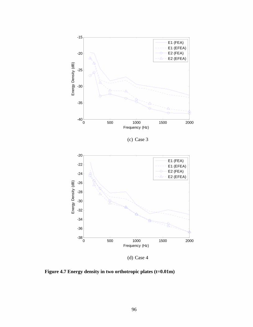
96
(c) Case 3
(d) Case 4
Figure 4.7 Energy density in two orthotropic plates (t=0.01m)
0 500 1000 1500 2000-40
-35
-30
-25
-20
-15
Frequency (Hz)
Ene
rgy
Den
sity
(dB
)
E1 (FEA)E1 (EFEA)E2 (FEA)E2 (EFEA)
0 500 1000 1500 2000-38
-36
-34
-32
-30
-28
-26
-24
-22
-20
Frequency (Hz)
Ene
rgy
Den
sity
(dB
)
E1 (FEA)E1 (EFEA)E2 (FEA)E2 (EFEA)

97
From Figure 4.7, we can see that for the similar orientation (case 1 and 4), the
EFEA model matches well with the results from FEA. For the cases of dissimilar
orientation (case 2 and 3), however, the EFEA model overestimates the bending wave
transmission from plate 1 to plate 2. This phenomenon can be explained by the fact that
the two models (EFEA model and FEA model) consider different coupling between
eigenmodes (Bosmans, Mees et al. 1996). The FEA model predicts the actual coupling
between the eigenmodes of the two plates; however, the EFEA model assumes that every
mode of the first plate is evenly coupled to every mode of the second plate. This
assumption is valid for the cases of similar orientation, because the eigenmodes have the
same shape in two plates. For the cases of dissimilar orientation, the eigenmodes have
different shapes in two plates; the assumption made by EFEA is no long valid.
To validate this explanation, we increase the modal density of the plates by
reducing the thickness from 0.01m to 0.001m and increasing the frequency range to 5000
Hz. The results are shown in Figure 4.8.
0 1000 2000 3000 4000 5000
-15
-10
-5
0
5
10
Frequency (Hz)
Ene
rgy
Den
sity
(dB
)
E1 (FEA)E1 (EFEA)E2 (FEA)E2 (EFEA)

98
(a) Case 1
(b) Case 2
(c) Case 3
0 1000 2000 3000 4000 5000-20
-15
-10
-5
0
5
10
Frequency (Hz)
Ene
rgy
Den
sity
(dB
)
E1 (FEA)E1 (EFEA)E2 (FEA)E2 (EFEA)
0 1000 2000 3000 4000 5000-20
-15
-10
-5
0
5
10
Frequency (Hz)
Ene
rgy
Den
sity
(dB
)
E1 (FEA)E1 (EFEA)E2 (FEA)E2 (EFEA)

99
(d) Case 4
Figure 4.8 Energy density in two orthotropic plates (t=0.001m)
In Figure 4.8, much better agreements between FEA and EFEA models can be
observed for all the four cases. Especially for the cases of dissimilar orientation (case 2
and 3), with the increasing frequency, the difference between FEA and EFEA results of
energy density level of the two plates dropped from 3 dB to 0 dB. The reason for this
better agreement is that with the increased modal density of the plates, the coupling
between the modes also increased, especially for the differently orientated plates.
0 1000 2000 3000 4000 5000-20
-15
-10
-5
0
5
10
Frequency (Hz)
Ene
rgy
Den
sity
(dB
)
E1 (FEA)E1 (EFEA)E2 (FEA)E2 (EFEA)

100
Chapter 5
POWER TRANMISSION THROUGH COUPLED COMPOSITE LAMINATE
PLATES
5.1 Introduction
Composite laminate plates are increasingly used to construct structures or
structural components because of their high specific mechanical properties and light
weight. In order to evaluate the power flow within such structures at high frequency, the
power transmission characteristic of the junctions where two or more composite laminate
plates are connected together needs to be studied.
In Chapter 4, the power transmission coefficient and joint matrix for coupled
orthotropic plates was derived. In this chapter, the power transmission mechanism at the
junctions of general composite laminate plates is studied following the similar approach
as discussed in Chapter 4. First, the governing equations for the bending and in-plane
vibrations of composite laminate plate are presented. The solutions to the governing
equations are derived, with emphasis on derivation of in-plane wavenumbers. Second, the
expression of wave dynamic stiffness matrix is derived. Then, the complete equations at
the junction, with contribution from each semi-infinite plate is formed and solved. The
displacement in each plate can be found and the power transmission coefficients can be

101
calculated. Third, the joint matrix is formed and the global system of EFEA matrix is
assembled. Finally, numerical examples are given and comparison between EFEA
formulation and very dense FEA model is presented.
5.2 Derivation of Power Transmission Coefficients
5.2.1 Governing equations
Compared to the equations of motion for orthotropic plate, the equations of
motion for the composite laminate plate have additional terms , , , . These
terms gives the coupling between bending and torsion(Whitney and Ashton 1987).
4 2 2 4 0
(5.1)
2 0
(5.2)
2 0
(5.3)
where etc. are the coefficients of bending stiffness matrices of th plate, etc.
are the coefficients of extensional stiffness matrices of th plate.
The relationship between the displacements and the traction that act at the
connected edge of the plate can be expressed as follows (Whitney and Ashton 1987). The
tractions that act on the common edge of the plates are evaluated at 0.
2 (5.4)
2 3 (5.5)

102
(5.6)
(5.7)
The forces and moments per unit length at the junction can be expressed as the
summation of the product of transformation matrix and the tractions at each plate
(Langley and Heron 1990). It can be expressed as:
∑ (5.8)
where represents the tractions that act at the connected edge of plate
, and the transformation matrix is given by:
1 00 cos
0 0sin 0
0 sin0 0
cos 0 0 1
(5.9)
where is the angle of the local coordinate in plate with respect to the global
coordinate system.
Similar to Chapter 4, the compatibility conditions between the junction
displacement , and the edge displacement of plate , require that
(5.10)
where ,
5.2.2 Derivation of in-plane wavenumbers for composite laminate plates
Because of the anisotropy of composite laminate plate, the velocity of the mode is
dependent on the direction of wave propagation (Bosmans, Mees et al. 1996; Bosmans,
Vermeir et al. 2002). The dispersion relationship will again be obtained by assuming a
plane wave form of the displacement and substituting into the equations of motion. Same

103
as the orthotropic case, the in-plane displacements for composite laminate plates are
given by (Prosser 1991):
cos sin (5.11)
cos sin (5.12)
where and are the amplitudes of the two in-plane motions, is the direction
of the wave propagation.
Substituting these displacements into the equations of motion yields:
22
0
(5.13)
where cos , sin .
Setting the determinant equal to zero will yield a quadratic equation of . The
two solutions of group velocity correspond to the quasi-longitudinal and quasi-shear
modes. Generally, the quasi-longitudinal mode is faster and thus corresponds to the
smaller root.
5.2.3 Derivation of dynamic stiffness matrix
Assume the out-of-plane displacement of plate has the form of exp
, can be expressed as:
(5.14)
where is
the bending wavenumber (Langley 1996), it depends on the direction of wave
propagation .
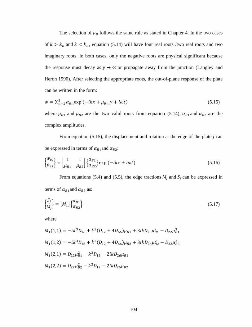
104
The selection of follows the same rule as stated in Chapter 4. In the two cases
of and , equation (5.14) will have four real roots /two real roots and two
imaginary roots. In both cases, only the negative roots are physical significant because
the response must decay as ∞ or propagate away from the junction (Langley and
Heron 1990). After selecting the appropriate roots, the out-of-plane response of the plate
can be written in the form:
∑ exp (5.15)
where and are the two valid roots from equation (5.14), and are the
complex amplitudes.
From equation (5.15), the displacement and rotation at the edge of the plate can
be expressed in terms of and :
1 1 exp (5.16)
From equations (5.4) and (5.5), the edge tractions and can be expressed in
terms of and as:
(5.17)
where
1,1 4 3
1,2 4 3
2,1 2
2,2 2

105
Eliminate and from equation (5.17) using equation (5.16), we can get the
following relationship between the edge displacements , and the edge tractions
and :
(5.18)
where
1,1 3
1,2 4 3
2,1
2,2 2
Similar procedure can be used to determine the in-plane behavior of the plate.
Assuming the in-plane motions are in the following expressions:
(5.19)
(5.20)
where is the ratio between the amplitudes of the two displacements.
Substituting equation (5.19) and (5.20) into the in-plane equations of motion, we
can get the following expression:
22
1 00 (5.21)
Take the determinant equal to zero yield a polynomial equation of . Again,
among the four roots of only the real and negative or imaginary and negative roots are
selected. They are the corresponding components of longitudinal and shear
wavesnumbers respectively. Associated with each root is a mode shape which governs

106
the relationship between the two in-plane displacements. The two mode shapes can also
be obtained as 1 and 1 .
Thus, the in-plane response can be written in the form:
1 eµL1 eµS exp (5.22)
where and are the complex amplitudes of the associated complementary functions.
Thus, the edge displacements and can be also expressed in terms of and as:
1 1 exp (5.23)
Similarly, we can express the edge tractions and in terms of and as:
(5.24)
where
1,1
1,2
2,1
2,2
Eliminate and from equation (5.24) using equation (5.23), we can get the
following relationship between the edge displacements , and the edge
tractions and :
(5.25)
where
1,1

107
1,2
2,1
2,2
Equations (5.18) and (5.25) can be combined to produce a relationship between
the complete set of edge displacements and tractions of the form:
(5.26)
where
,
,
The entries of dynamic stiffness matrix have been derived and can be found
from equation (5.18) and (5.25) as:
1,1 1,22,1 2,2
0 00 0
0 00 0
1,1 1,22,1 2,2
(5.27)
5.2.4 Assembly of the complete equations and the calculation of transmission coefficients
The assembly of the complete equations and the calculation of transmission
coefficients of the composite laminate plate follows the same procedure as described in
Chapter 4. The averaged power transmission coefficient can be obtained by
integrating the angle of incidence from 0 to .
, sin (5.28)

108
5.3 Derivation of Joint Matrix
The derivation of joint matrix for composite laminate plates will also follow the
same procedure as in Chapter 4. The joint matrix expression for the coupled composite
laminate plates appears same as equation (4.62), but the entries of the joint matrix is
calculated using the power transmission coefficients derived in this Chapter.
5.4 Assembly of Global EFEA Equations for Coupled Composite Laminate Plates
The matrix expression of EFEA differential equation for single composite
laminate plate at the element level is obtained in Chapter 3 and it can be expressed as:
,, , , (5.29)
where subscript 1 corresponds to the stiffness coefficients , , , , which
correspond to the orthotropic plate, and the subscripts 2 corresponds to the stiffness
and .
Using the alternative approach for developing the EFEA differential equation for
composite laminate plate by finding the equivalent isotropic material, the EFEA
differential equation at element level can be expressed as:
(5.30)
The power flow can be expressed in terms of energy density and power
transmission coefficients.
(5.31)
109
where and 1 represents the two nodes of the element at the joint, and 1
represents the two nodes of the element at the joint, the joint matrices define the
power transfer across elements at the joints.
The final assembled system of EFEA equations can be expressed as:
(5.32)
where and are the element matrix for the and element, and are
the vectors containing all the nodal degrees of freedom for elements and .
5.5 Numerical Examples and Validation
In this section, an L-junction of two composite laminate plates is modeled using
EFEA and conventional FEA and the results of energy distribution in two plates from
both methods are compared.
The properties of the fiber composites that are used to compose the laminate
plates are:
Carbon/Epoxy:
138 , 8.96 , 7.10 , 0.30, 1600 / (5.33)
E-glass/Epoxy:
39 , 8.6 , 3.8 , 0.28, 2100 / (5.34)
The first composite laminate plate is composed of three layers of carbon/epoxy
fiber composites. The thickness of each layer is 1mm. The orientation of the composite is
shown in Figure 5.1.

110
Figure 5.1 The orientation of the first composite laminate plate
The extensional and bending stiffness matrices of the first plate can be obtained
from the orientation and properties of each ply and can be expressed as:
30.9 5.09 8.095.09 4.92 3.158.09 3.15 6.41
10 / (5.35)
196 52.4 87.652.4 44.3 34.187.6 34.1 62.3
· (5.36)
The second composite laminate plate is composed of two layers of e-glass/epoxy
fiber composites. The orientation of the composite is shown in Figure 5.2.
Figure 5.2 The orientation of the second composite laminate plate
The extensional and bending stiffness matrices of the first plate can be obtained
from the orientation and properties of each ply and can be expressed as:
28.4 5.99 3.875.99 12.9 3.873.87 3.87 7.34
10 / (5.37)

th
th
re
th
5
m
F
th
F
2.370.4990.322
For th
hese two cas
he first case,
eference coo
he edge with
The m
.3 (a) and (b
model in EFE
Figure 5.3 Th
In the
he energy de
EA model a
0.499 01.08 0
0.322 0
his L-junctio
ses, the seco
, the second
ordinate; in t
h 90 degree t
models in the
b) respective
EA has only
he models o
calculation,
ensity of pla
and the EFEA
0.3220.3220.612
·
on of two com
ond plate is c
plate is con
the second c
to the referen
e convention
ely. The mo
32 elements
(a)
of orthotrop
, plate 1 is g
ate 1 and pl
A formulatio
111
mposite lam
connected to
nnected to fir
ase, the seco
nce coordina
nal FEA and
odel in conv
s.
pic L-junctio
given excitati
late 2 in two
ons respectiv
minate plates
o the differe
rst plate at t
ond plate is c
ate.
d EFEA form
ventional FE
on in conven
ion on three
o cases is c
vely. The po
, two cases a
nt edges of
the edge wit
connected to
mulation are
EA has 12,80
(b)
ntional FEA
randomly se
alculated us
wer transmi
(5
are calculate
the first pla
th 0 degree t
o the first pla
shown in F
00 elements
A and EFEA
elected locat
sing convent
ssion mecha
.38)
ed. In
te. In
to the
ate at
Figure
. The
A
tions,
tional
anism

112
derived for composite laminate plates is used in the calculation. For the conventional
finite element analysis, the velocity at each node within the plate is obtained through
dynamic analysis. First, the input power can be computed from FEA model at the
excitation locations and the computed input power serve as the excitation applied in the
EFEA model at the corresponding locations. Then, the energy density level of the plate is
computed from the velocity value and then averaged over the entire plate (spatial
average) and over the 1/3 octave band (frequency average). The averaged energy density
level obtained from FEA model is then compared with the energy density computed from
EFEA formulation. The comparison is shown in Figure 5.4 – 5.5.
Figure 5.4 Comparison of energy density between EFEA and conventional FEA
(case 1)
0 1000 2000 3000 4000 5000-30
-25
-20
-15
-10
-5
0
Frequency (Hz)
Ene
rgy
Den
sity
(dB
)
E1 (FEA)E1 (EFEA)E2 (FEA)E2 (EFEA)

113
Figure 5.5 Comparison of energy density between EFEA and conventional FEA
(case 2)
The velocity difference between these two plates is also calculated using two
models. The velocity difference is defined as (Bosmans, Mees et al. 1996):
10log ⁄ (5.39)
The velocity difference between the two plates is computed using two methods
and is shown in Figure 5.6 and 5.7.
0 1000 2000 3000 4000 5000-35
-30
-25
-20
-15
-10
-5
0
5
Frequency (Hz)
Ene
rgy
Den
sity
(dB
)
E1 (FEA)E1 (EFEA)E2 (FEA)E2 (EFEA)

114
Figure 5.6 Comparison of velocity difference between two plates (case 1)
Figure 5.7 Comparison of velocity difference between two plates (case 2)
From the comparison plots, we find good agreements between the EFEA results
and the results from very dense FEA model. The difference of the results obtained from
0 1000 2000 3000 4000 50002
3
4
5
6
7
8
9
10
11
12
Frequency (Hz)
Vel
ocity
Diff
eren
ce (d
B)
FEAEFEA
0 1000 2000 3000 4000 50004
5
6
7
8
9
10
11
12
13
14
Frequency (Hz)
Vel
ocity
Diff
eren
ce (d
B)
FEAEFEA

115
two models is within 1.5 dB. For the two different cases when the second plate is
connected to the different edges of the first plate, the energy density level and velocity
difference level have about 3 dB difference. This phenomenon is expected because of the
anisotropy of the composite laminate plate.

116
Chapter 6
CONCLUSIONS AND RECOMMENDATIONS FOR FUTURE WORK
6.1 Conclusions
EFEA has been proven to be an effective and reliable tool for high frequency
vibration analysis. It uses the averaged energy variable as the primary variable to form
the governing differential equations and provides a practical approach to evaluate the
structural response at high frequencies, which is hard to reach with conventional finite
element analysis because of the computational cost. In the past, EFEA has been applied
successfully to different structures, such as beams, rods, plates, curved panels etc. Until
recently, however, not much work has been done in the field of composite structures.
The new developments of EFEA formulations in composite laminate plates are
presented in this dissertation. The EFEA governing differential, with the time- and
space- averaged energy density as the primary variable, is developed for general
composite laminate plates. The power transmission characteristics at plate junctions of
non-isotropic materials, including orthotropic plates and composite laminate plates are
studied in order to assemble to global system of EFEA equations for complex structures.
The major work of this dissertation is:

117
1. The EFEA differential equation for single composite laminate plate is derived. The
equations of motions that govern the vibration of composite laminate plate are
presented. Convergence study is proceeded to prove the fact that the coupling terms
between bending and in-plane motions become insignificant in high frequency range.
The out-of-plane and in-plane equations of motions are thus considered uncoupled in
our derivation. The wave solutions for the out-of-plane and in-plane displacements
and the corresponding dispersion relationships are obtained. The expressions of
energy density and energy intensities are derived and the relationship between the
time- and space- averaged energy density and intensities is found, this relation,
together with the power balance in a differential control volume of the plate, are
utilized to form the EFEA differential equation with the energy density as the primary
variable. The EFEA differential equation is derived for both bending and in-plane
wave motion of the plate. Some numerical examples are presented where the EFEA
model is validated by comparing with very dense FEA model. Finally, an alternative
approach of forming the EFEA differential equation for composite laminate plates is
introduced by using its equivalent isotropic plate and some validation is presented.
2. The power transmission for coupled orthotropic plates is studied. In the model, an
arbitrary number of orthotropic plates are connected at a common edge. The power
transmission coefficients are derived using the wave propagation approach. It
assumes the wave propagates in the semi-infinite plate and is partially reflected and
partially transmitted to other plates through the junction. The wave dynamic stiffness
matrix is derived for each semi-infinite plate and the appropriate equilibrium and
compatibility conditions at the junction are utilized to form the complete equation at

118
the junction. This equation is solved to obtain the displacements in each plate and the
wave amplitudes of each type of waves that has been reflected or transmitted. The
power transmission coefficients can then be computed. The power transmission
coefficients are dependent on the angle of incident wave, thus, the final coefficients
are averaged over all the angles of incidence. The joint matrix is then derived and the
global system of EFEA equations are formed for coupled orthotropic plates. Finally,
some numerical examples are studied to validate the derivation.
3. The power transmission for coupled composite laminate plates is also studied. The
derivation of power transmission coefficients is also based on the same procedure
assuming the propagation of elastic waves in semi-infinite composite laminate plates.
Numerical example of two general composite laminate plates connected at junction is
studied and the EFEA formulation is validate through comparing the results with the
results from very dense FEA model.
6.2 Recommendations for Future Work
This dissertation summarized the work regarding to the application of energy
finite element analysis to composite laminate plates. There are several possible
developments for future work:
1. In the development of energy finite element formulations in composite laminate
plates, classical laminate theory is used. This theory, however, is not accurate enough
for thick composite plates, in which the shear resultants cannot be neglected. Thus,
some other theories, such as shear deformation theory and layer by layer theory can
be used for thick composite plates by accounting for the transverse shear deformation
and the shear discontinuity through the plate thickness.

119
2. The main part of the derivation that has been done in this dissertation is written in
MATLAB program. A FORTRAN program is needed in order to make this part of
EFEA formulation work effectively with the main EFEA program. This will enable
us to model the complex structures using finite element pre-processor and solve for
the energy density distribution using the EFEA program effectively.
3. There are other forms of composite structures that are also widely used in the
industries. The application of EFEA formulation to these types of structures, such as
composite sandwich plate, thick composite plates, composite beams, composite
panels etc. is very necessary and important.
4. Stiffeners are often used at junctions in the construction of composite structures. The
EFEA formulation can be extended to account for the presence of stiffeners at the
junction between composite panels.
5. The high frequency vibration analysis of composite structures under heavy fluid
loading. Previously, this analysis has been done in thin isotropic plates and the
extension of this research to the field of composite plates is meaningful for the NVH
analysis of composite marine structures.
6. The development of hybrid finite element formulation for composite structures. The
hybrid finite element method provides an approach for evaluating the vibration in the
mid-frequency range. This development will give valuable significance to assess the
response of composite structures at mid-frequencies.

120
APPENDIX
Derivation of Time- and Space- averaged Energy Density and Intensities for
Composite Laminate Plates
A.1 Derivation of Time- and Space- averaged Energy Density
In equation (3.24), the time-averaged energy density for composite laminate
plates can be expressed as:
2 4
4 4 (A.1)
The far-field displacement solution for the bending vibration of the plate can be
expressed as:
, , (A.2)
Substituting (A.2) into (A.1), we get the following expression:
| | 2 |
| 4 | | | | 4
4
(A.3)
where means exp .

121
In equation (A.3), the term | | can be expanded as:
| | | | | | | | | |
(A.4)
In order to get the space-averaged energy density, we need to average the energy
density value over a half wavelength as:
⁄ ⁄ (A.5)
The integral for the first term in equation (A.4) becomes:
| |2 ⁄ ⁄ | |
⁄ ⁄ (A.6)
If the damping is very small ( 1), the exponential function in (A.6) can be
assumed to be constant on the interval (Park, Hong et al. 2003):
| | ⁄ ⁄ | |
⁄ ⁄ | |
(A.7)
The other similar terms | | , | | , | | can also be integrated
similarly and get similar results as in (A.7).
The integral for the other terms such as can be obtained as:
⁄ ⁄ ⁄ ⁄ 0
(A.8)
Thus, the time- and space- averaged energy density can be expressed as:
| | 2 4 | | | |

122
| | | | | | 4 4 | |
| | | | | | (A.9)
Substituting 1 , 1 and 1
, 1 etc. into equation (A.9), and neglecting all the second and higher
order terms of the damping loss factor, the terms can be simplified as:
| | 2 4 | |
1 2 1 1 4 1
2 2 (A.10)
4 4 4 1
4 (A.11)
Thus, the time- and space- averaged energy density can be expressed as:
14 2 2 | | | |
| | | |
| | | | | | | |
(A.12)
where represents .
A.2 Derivation of Time- and Space- averaged Energy Intensities
The and components of the time-averaged intensity of a laminated plate can
be expressed as:
123
(A.13)
(A.14)
Substituting the forces and moments into equation (A.13) yields the expression
for the x component of the energy intensity as:
2 3
2
2 (A.15)
Substituting the far-field solution into equation (A.15), and taking the space
average of the energy intensity by integrating it over a half wavelength, we get the time-
and space- averaged energy intensity as:
2
2 | | | | | | | | 3
2 | | | | | | | |
(A.16)
Again, substituting 1 , 1 and
1 , 1 etc. into equation (A.16), and neglecting all the second
and higher order terms of the damping loss factor, the terms can be simplified as:
2 2 2
2 2 (A.17)
124
3 2 6
2 (A.18)
Thus, the x component of the time- and space- averaged energy intensity can be
expressed as:
2 | | | | | | | |
3 | | | | | | | |
(A.19)
Similarly, the y component of the time- and space- averaged energy intensity can
be expressed as:
2 | | | | | | | |
3 | | | | | | | |
(A.20)

125
REFERENCES
1. Agarwal, B. D. and L. J. Broutman (1990). Analysis and Performance of Fiber
Composites. New York, Wiley.
2. Ashton, J. E. and J. M. Whitney (1970). Theory of Laminated Plates. Stamford,
Conn., Technomic.
3. Auld, B. A. (1990). Acoustic Fields and Waves in Solids. Malabar, Fla., R.E.
Krieger.
4. Bernhard, R. J. and J. E. Huff (1999). "Structural-Acoustic Design at High
Frequency using the Energy Finite Element Method." Journal of Vibration and
Acoustics-Transactions of the ASME 121(3): 295-301.
5. Bitsie, F. and R. J. Bernhard (1996). The Structural-Acoustic Energy Finite
Element Method and Energy Boundary Element Method. West Lafayette, Purdue
Univeristy.
6. Bosmans, I., P. Mees, et al. (1996). "Structure-borne sound transmission between
thin orthotropic plates: Analytical solutions." Journal of Sound and Vibration
191(1): 75-90.
7. Bosmans, I. and T. R. T. Nightinghale (1999). Structure-borne Sound
Transmission in Rib-stiffened Plate Structures Typical of Wood Frame Buildings.

126
Ontario, National Research Council Canada, Institute for Research in
Construction Acoustics.
8. Bosmans, I., G. Vermeir, et al. (2002). "Coupling Loss Factors for Coupled
Anisotropic Plates." Journal of Sound and Vibration 250(2): 351-355.
9. Bouthier, O. M. (1992). Energetics of Vibrating Systems. Mechanical
Engineering Department. West Lafayette, Purdue University. Ph.D. Dissertation.
10. Bouthier, O. M. and R. J. Bernhard (1992). "Models of Space-Averaged
Energetics of Plates." AIAA Journal 30(3): 616-623.
11. Bouthier, O. M. and R. J. Bernhard (1995). "Simple-Models of Energy-Flow in
Vibrating Membranes." Journal of Sound and Vibration 182(1): 129-147.
12. Bouthier, O. M. and R. J. Bernhard (1995). "Simple-Models of the Energetics of
Transversely Vibrating Plates." Journal of Sound and Vibration 182(1): 149-166.
13. Chakraborty, A., D. R. Mahapatra, et al. (2002). "Finite Element Analysis of Free
Vibration and Wave Propagation in Asymmetric Composite Beams with
Structural Discontinuities." Composite Structures 55(1): 23-36.
14. Cho, P. E. (1993). Energy Flow Analysis of Coupled Structures. Mechanical
Engineering Department. West Lafayette, Purdue University. Ph. D. Dissertation.
15. Cho, P. E. and R. J. Bernhard (1998). "Energy Flow Analysis of Coupled Beams."
Journal of Sound and Vibration 211(4): 593-605.
16. Crandali, S. H. and R. Lotz (1971). "On the Coupling Loss Factor in Statistical
Energy Analysis." The Journal of the Acoustical Society of America 49(1): 354-
356.

127
17. Craven, P. G. and B. M. Gibbs (1981). "Sound-Transmission and Mode-Coupling
at Junctions of Thin Plates .1. Representation of the Problem." Journal of Sound
and Vibration 77(3): 417-427.
18. Cremer, L., M. Heckl, et al. (1973). Structure Born Sound, Springer-Verlag.
19. DeLanghe, K., P. Sas, et al. (1997). "The Use of Wave-Absorbing Elements for
the Evaluation of Transmission Characteristics of Beam Junctions." Journal of
Vibration and Acoustics-Transactions of the ASME 119(3): 293-303.
20. Fahy, F. J. (1982). Noise and Vibration, Chichester: Ellis Horwood.
21. Fahy, F. J. (1994). "Statistical Energy Analysis - a Critical Overview."
Philosophical Transactions of the Royal Society of London Series a-Mathematical
Physical and Engineering Sciences 346(1681): 431-447.
22. Fredo, C. R. (1997). "A SEA-like Approach for the Derivation of Energy Flow
Coefficients with a Finite Element Model." Journal of Sound and Vibration
199(4): 645-666.
23. Gibbs, B. M. and P. G. Craven (1981). "Sound-Transmission and Mode-Coupling
at Junctions of Thin Plates .2. Parametric Survey." Journal of Sound and
Vibration 77(3): 429-435.
24. Heckl, M. (1962). "Vibrations of Point-Driven Cylindrical Shells." Journal of the
Acoustical Society of America 34(10): 1553-1557.
25. Her, S. C. and Y. C. Liang (2004). "The Finite Element Analysis of Composite
Laminates and Shell Structures subjected to Low Velocity Impact." Composite
Structures 66(1-4): 277-285.

128
26. Horner, J. L. and R. G. White (1990). "Prediction of Vibrational Power
Transmission through Jointed Beams." International Journal of Mechanical
Sciences 32(3): 215-223.
27. Iannucci, L. and J. Ankersen (2006). "An Energy Based Damage Model for Thin
Laminated Composites." Composites Science and Technology 66(7-8): 934-951.
28. Jones, R. M. (1999). Mechanics of Composite Materials. Philadelphia, PA, Taylor
& Francis.
29. Kim, H. S., H. J. Kang, et al. (1994). "A Vibration Analysis of Plates at High-
Frequencies by the Power-Flow Method." Journal of Sound and Vibration 174(4):
493-504.
30. Koh, C. G., K. K. Ang, et al. (2003). "Dynamic Analysis of Shell Structures with
Application to Blast Resistant Doors." Shock and Vibration 10(4): 269-279.
31. Krishnamurthy, K. S., P. Mahajan, et al. (2003). "Impact Response and Damage
in Laminated Composite Cylindrical Shells." Composite Structures 59(1): 15-36.
32. Langley, R. S. (1989). "A General Derivation of the Statistical Energy Analysis
Equations for Coupled Dynamic-Systems." Journal of Sound and Vibration
135(3): 499-508.
33. Langley, R. S. (1990). "A Derivation of the Coupling Loss Factors Used in
Statistical Energy Analysis." Journal of Sound and Vibration 141(2): 207-219.
34. Langley, R. S. (1994). "Elastic-Wave Transmission Coefficients and Coupling
Loss Factors for Structural Junctions between Curved Panels." Journal of Sound
and Vibration 169(3): 297-317.

129
35. Langley, R. S. (1996). "The Modal Density of Anisotropic Structural
Components." Journal of the Acoustical Society of America 99(6): 3481-3487.
36. Langley, R. S. and P. Bremner (1999). "A Hybrid Method for the Vibration
Analysis of Complex Structural-acoustic Systems." Journal of the Acoustical
Society of America 105(3): 1657-1671.
37. Langley, R. S. and K. H. Heron (1990). "Elastic Wave Transmission through
Plate Beam Junctions." Journal of Sound and Vibration 143(2): 241-253.
38. Langley, R. S., J. R. D. Smith, et al. (1997). "Statistical Energy Analysis of
Periodically Stiffened Damped Plate Structures." Journal of Sound and Vibration
208(3): 407-426.
39. Lyon, R. (1975). Statistical Energy Analysis of Dynamical Systems: Theory and
Application. Cambridge, The MIT Press.
40. Lyon, R. H. and E. Eichler (1964). "Random Vibration of Connected Structures."
Journal of the Acoustical Society of America 36(7): 1344-1356.
41. Lyon, R. H. and G. Maidanik (1962). "Power Flow between Linearly Coupled
Oscillators." Journal of the Acoustical Society of America 34(5): 623-630.
42. Mahapatra, D. R. and S. Gopalakrishnan (2004). "Spectral Finite Element
Analysis of Coupled Wave Propagation in Composite Beams with Multiple
Delaminations and Strip Inclusions." International Journal of Solids and
Structures 41(5-6): 1173-1208.
43. Maidanik, G. (1962). "Response of Ribbed Panels to Reverberant Acoustic
Fields." Journal of the Acoustical Society of America 34(6): 809-815.
130
44. Manning, J. E. and G. Maidanik (1964). "Radiation Properties of Cylindrical
Shells." Journal of the Acoustical Society of America 36(9): 1691-1700.
45. Mccollum, M. D. and J. M. Cuschieri (1990). "Thick Plate Bending Wave
Transmission Using a Mobility Power Flow Approach." Journal of the Acoustical
Society of America 88(3): 1472-1479.
46. Mees, P. and G. Vermeir (1993). "Structure-Borne Sound-Transmission at
Elastically Connected Plates." Journal of Sound and Vibration 166(1): 55-76.
47. Meo, M., R. Vignjevic, et al. (2005). "The Response of Honeycomb Sandwich
Panels under Low-velocity Impact Loading." International Journal of Mechanical
Sciences 47(9): 1301-1325.
48. Nayakl, A. K., R. A. Shenoi, et al. (2006). "Dynamic Response of Composite
Sandwich Plates subjected to Initial Stresses." Composites Part A-Applied
Science and Manufacturing 37(8): 1189-1205.
49. Nefske, D. J. and S. H. Sung (1989). "Power Flow Finite-Element Analysis of
Dynamic-Systems - Basic Theory and Application to Beams." Journal of
Vibration Acoustics Stress and Reliability in Design-Transactions of the ASME
111(1): 94-100.
50. Oguibe, C. N. and D. C. Webb (1999). "Finite-element Modelling of the Impact
Response of a Laminated Composite Plate." Composites Science and Technology
59(12): 1913-1922.
51. Park, D. H., S. Y. Hong, et al. (2003). "Power Flow Model of Flexural Waves in
Finite Orthotropic Plates." Journal of Sound and Vibration 264(1): 203-224.

131
52. Park, D. H., S. Y. Hong, et al. (2001). "Power Flow Models and Analysis of In-
plane Waves in Finite Coupled Thin Plates." Journal of Sound and Vibration
244(4): 651-668.
53. Pierre, C., N. Vlahopoulos, et al. (2004). "Advanced Structure Methodologies for
Next-generation Ground Vehicles, Part 1: Basic Theories." International Journal
of Heavy Vehicle Systems 11(3-4): 257-281.
54. Pierre, C., N. Vlahopoulos, et al. (2004). "Advanced Structure Methodologies for
Next-generation Ground Vehicles, Part 2: Case Study." International Journal of
Heavy Vehicle Systems 11(3-4): 282-302.
55. Prosser, W. H. (1991). The Propagation Characteristics of the Plate Modes of
Acoustic Emission Waves in Thin Aluminum Plates and Thin Graphite/epoxy
Composite Plates and Tubes, The Johns Hopkins Univsersity. Ph.D. Dissertation.
56. Qiu, X., V. S. Deshpande, et al. (2003). "Finite Element Analysis of the Dynamic
Response of Clamped Sandwich Beams subject to Shock Loading." European
Journal of Mechanics 22(6): 801-814.
57. Reddy, J. N. (1997). Mechanics of Laminated Composite Plates : Theory and
Analysis. Boca Raton, CRC Press.
58. Reddy, J. N. (2004). Mechanics of Laminated Composite Plates and Shells :
Theory and Analysis. Boca Raton, CRC Press.
59. Renji, K., P. S. Nair, et al. (1996). "Modal Density of Composite Honeycomb
Sandwich Panels." Journal of Sound and Vibration 195(5): 687-699.

132
60. Rostam-Abadi, F., C. M. Chen, et al. (2000). "Design Analysis of Composite
Laminate Structures for Light-weight Armored Vehicle by Homogenization
Method." Computers & Structures 76: 319-335.
61. Sablik, M. J. (1982). "Coupling Loss Factors at a Beam L-Joint Revisited."
Journal of the Acoustical Society of America 72(4): 1285-1288.
62. Simmons, C. (1991). "Structure-Borne Sound-Transmission through Plate
Junctions and Estimates of Sea Coupling Loss Factors Using the Finite-Element
Method." Journal of Sound and Vibration 144(2): 215-227.
63. Smith, P. W. (1962). "Response and Radiation of Structural Modes Excited by
Sound." Journal of the Acoustical Society of America 34(5): 640-650.
64. Steel, J. A. and R. J. M. Craik (1994). "Statistical Energy Analysis of Structure-
Borne Sound-Transmission by Finite-Element Methods." Journal of Sound and
Vibration 178(4): 553-561.
65. Szecheny, E. (1971). "Modal Densities and Radiation Efficiencies of Unstiffened
Cylinders Using Statistical Methods." Journal of Sound and Vibration 19(1): 65-
81.
66. Vaziri, R., X. Quan, et al. (1996). "Impact Analysis of Laminated Composite
Plates and Shells by Super Finite Elements." International Journal of Impact
Engineering 18(7-8): 765-782.
67. Vlahopoulos, N., L. O. Garza-Rios, et al. (1999). "Numerical Implementation,
Validation, and Marine Applications of an Energy Finite Element Formulation."
Journal of Ship Research 43(3): 143-156.

133
68. Vlahopoulos, N. and X. Zhao (1999). "Basic Development of Hybrid Finite
Element Method for Midfrequency Structural Vibrations." AIAA Journal 37(11):
1495-1505.
69. Vlahopoulos, N. and X. Zhao (2001). "An Investigation of Power Flow in the
Mid-frequency Range for Systems of Co-linear Beams based on a Hybrid Finite
Element Formulation." Journal of Sound and Vibration 242(3): 445-473.
70. Vlahopoulos, N., X. Zhao, et al. (1999). "An Approach for Evaluating Power
Transfer Coefficients for Spot-welded Joints in an Energy Finite Element
Formulation." Journal of Sound and Vibration 220(1): 135-154.
71. Whitney, J. M. and J. E. Ashton (1987). Structural Analysis of Laminated
Anisotropic Plates. Lancaster, Pa., U.S.A., Technomic Pub. Co.
72. Wilkinson, J. P. (1968). "Modal Densities of Certain Shallow Structural
Elements." Journal of the Acoustical Society of America 43(2): 245-256.
73. Wohle, W., T. Beckmann, et al. (1981). "Coupling Loss Factors for Statistical
Energy Analysis of Sound-Transmission at Rectangular Structural Slab Joints .1."
Journal of Sound and Vibration 77(3): 323-334.
74. Wohle, W., T. Beckmann, et al. (1981). "Coupling Loss Factors for Statistical
Energy Analysis of Sound-Transmission at Rectangular Structural Slab Joints .2."
Journal of Sound and Vibration 77(3): 335-344.
75. Wohlever, J. C. (1988). Vibrational Power Flow Analysis of Rods and Beams.
Mechanical Engineering Department. West Lafayette, Purdue University. Ph.D.
Dissertation.

134
76. Wohlever, J. C. and R. J. Bernhard (1992). "Mechanical Energy-Flow Models of
Rods and Beams." Journal of Sound and Vibration 153(1): 1-19.
77. Wu, H. Y. T. and F. K. Chang (1989). "Transient Dynamic Analysis of Laminated
Composite Plates subjected to Transverse Impact." Computers & Structures
31(3): 453-466.
78. Zhang, W. G., N. Vlahopoulos, et al. (2005). "An Energy Finite Element
Formulation for High-frequency Vibration Analysis of Externally Fluid-loaded
Cylindrical Shells with Periodic Circumferential Stiffeners subjected to Axi-
symmetric Excitation." Journal of Sound and Vibration 282(3-5): 679-700.
79. Zhang, W. G., A. M. Wang, et al. (2003). "High-frequency Vibration Analysis of
Thin Elastic Plates under Heavy Fluid Loading by an Energy Finite Element
Formulation." Journal of Sound and Vibration 263(1): 21-46.
80. Zhang, W. G., A. M. Wang, et al. (2005). "A Vibration Analysis of Stiffened
Plates under Heavy Fluid Loading by an Energy Finite Element Analysis
Formulation." Finite Elements in Analysis and Design 41(11-12): 1056-1078.
81. Zhao, X. and N. Vlahopoulos (2000). "A Hybrid Finite Element Formulation for
Mid-frequency Analysis of Systems with Excitation Applied on Short Members."
Journal of Sound and Vibration 237(2): 181-202.
82. Zhao, X. and N. Vlahopoulos (2004). "A Basic Hybrid Finite Element
Formulation for Mid-frequency Analysis of Beams Connected at an Arbitrary
Angle." Journal of Sound and Vibration 269(1-2): 135-164.
Recommended