Energies 2013, 6, 3297-3322; doi:10.3390/en6073297
energies ISSN 1996-1073
www.mdpi.com/journal/energies
Article
Harmonic Propagation and Interaction Evaluation between Small-Scale Wind Farms and Nonlinear Loads
Guang-Long Xie *, Bu-Han Zhang, Yan Li and Cheng-Xiong Mao
State Key Laboratory of Advanced Electromagnetic Engineering and Technology, Huazhong University of
Science and Technology, Wuhan 430074, China; E-Mails: [email protected] (B.-H.Z.);
[email protected] (Y.L.); [email protected] (C.-X.M.)
* Author to whom correspondence should be addressed; E-Mail: [email protected];
Tel./Fax: +86-27-8754-2669.
Received: 25 April 2013; in revised form: 26 June 2013 / Accepted: 2 July 2013 /
Published: 5 July 2013
Abstract: Distributed generation is a flexible and effective way to utilize renewable
energy. The dispersed generators are quite close to the load, and pose some power quality
problems such as harmonic current emissions. This paper focuses on the harmonic
propagation and interaction between a small-scale wind farm and nonlinear loads in the
distribution grid. Firstly, by setting the wind turbines as P – Q(V) nodes, the paper
discusses the expanding Newton-Raphson power flow method for the wind farm. Then the
generalized gamma mixture models are proposed to study the non-characteristic harmonic
propagation of the wind farm, which are based on Gaussian mixture models, improved
phasor clustering and generalized Gamma models. After the integration of the small-scale
wind farm, harmonic emissions of nonlinear loads will become random and fluctuating due
to the non-stationary wind power. Furthermore, in this paper the harmonic coupled
admittance matrix model of nonlinear loads combined with a wind farm is deduced by
rigorous formulas. Then the harmonic propagation and interaction between a real wind
farm and nonlinear loads are analyzed by the harmonic coupled admittance matrix and
generalized gamma mixture models. Finally, the proposed models and methods are verified
through the corresponding simulation models in MATLAB/SIMULINK and PSCAD/EMTDC.
Keywords: harmonic propagation and interaction; small-scale wind farm; nonlinear load;
generalized gamma mixture models; admittance matrix model
OPEN ACCESS

Energies 2013, 6 3298
1. Introduction
Following the depletion of fossil energy, renewable energy generation is a fast growing area
nowadays. With the increasing installed wind power generation capacity, we need to find more
effective ways to utilize wind energy.
Different for large-scale wind farms integrated into the regular high voltage transmission line [1,2],
dispersed wind generators are more flexible. Small-scale wind farms usually consist of several
dispersed wind generators, which are directly connected to a medium or low voltage distribution grid [3].
This allows the effective utilization of the limited wind resource in cities or suburbs and shortens the
transmission distance. The small-scale wind farm is however quite close to the load, which can pose
some power quality problems such as voltage fluctuation and harmonic current emissions.
The system impedance in the distribution grid is highly resistive, and the voltage fluctuation at the
Point of Common Coupling (PCC) is strongly affected by wind power smoothing level [4,5]. Wind
power data are non-stationary random signals because of the variable wind speed and wind energy
conversion systems [6–8]. At the same time, the fluctuating fundamental power can affect the
controller of conversion systems and induce harmonics, so the harmonic current emissions of wind
generators are analyzed by stochastic assessment. New models and methods for harmonic propagation
and interaction issues can be verified in several simulation systems, such as MATLAB/SIMULINK,
PSCAD/EMTDC and HYPERSIM [9–11].
Harmonic current emissions of wind generators consist of characteristic and non-characteristic
harmonics. Characteristic harmonics are affected by the topology structure of converters and the
switch control strategy of converter valves, whereas non-characteristic harmonics are induced by the
inherent slot harmonics of wind turbines, nonsinusoidal distributions of the stator and rotor windings,
and operating conditions of converters and the outside power grids [12,13]. Non-characteristic
harmonics of different wind turbines are almost independent low-order harmonics, even for the doubly
fed induction generator and direct-drive permanent magnet generator.
In order to analyze the complex harmonic current emissions, Generalized Gamma Mixture Models
(GGMM) are proposed in this paper. GGMM consists of Gaussian mixture models, improved phasor
clustering and generalized Gamma models. GGMM divide the complicated probability distribution
functions (pdfs) of harmonic sources for the harmonic propagation and interaction study. On the other
hand, the port characteristics of nonlinear devices in the distribution gird become variable due to the
installed wind generation. Power electronic devices are normally nonlinear [14,15], and the AC/DC
converter is important for them. The DC side part can be a linear load, battery, and motor drives with
DC/AC inverters [16,17]. These nonlinear loads generate several kinds of harmonic emissions into the
power grid, and iterative harmonic analysis is the common way to study harmonic power flow [18]. In
order to analyze the harmonic power flow, accurate harmonic source modeling is necessary. The
predetermined and harmonic–voltage dependent current source models are both defective [14,18].
Reference [15] proposes a harmonic admittance matrix to reflect the relationship between the AC side
harmonic voltages and currents of a rectifier. The harmonic coupled admittance matrix model is
strictly deduced and adjusted for the harmonic interaction in this paper.
Therefore this paper focuses on the harmonic propagation and interaction between a small-scale
wind farm and nonlinear loads in the distribution grid. Harmonic emissions of nonlinear loads become

Energies 2013, 6 3299
random and fluctuant due to the non-stationary wind power, meanwhile wind harmonic emissions
make it more complex. In this paper, first the power flow expanding model of wind turbines based on
P − Q(V) characteristic is studied, and GGMM of harmonic current are proposed and described in
detail. The switching harmonic currents produced by the grid-side and rotor-side converters of are also
analyzed in depth. Then the harmonic admittance matrix models of nonlinear loads combined with the
wind farm are established to analyze the harmonic propagation and interactions. Finally, the
proposed models and methods are verified through a simulation model in MATLAB/SIMULINK
and PSCAD/EMTDC.
2. Power Flow and Harmonic Source Modeling of Wind Farm
2.1. Power Flow Modeling of Wind Farm
When a small-scale wind farm is installed in the distribution grid, the port characteristics of
nonlinear loads will become more complex. Compared to the variable loads, the small-scale wind farm
induces a fluctuating negative power flow, and supplies voltage to the distribution grid.
The most common forms of wind generation contain asynchronous generators (AGs), doubly-fed
induction generators (DFIGs) and direct-drive generators. In this paper, the DFIG is modeled to study
the harmonic propagation in the distribution grid. The topological diagram of the small-scale wind
farm is shown in Figure 1.
The steady state circuit model of DFIG is shown in Figure 2 [19]. The term ωe is the nominal
angular speed, ωs, ωr, ωm are the stator, rotor, and rotating angular speed, and N = ±1 represents the positive and negative circuit. When the fundamental power flow is studied, , 1s e Nω ω= = ,
e m
e
slip sω ω
ω−= = .
Figure 1. The topological diagram of the small-scale wind farm.
Figure 2. The steady state circuit model of DFIG.
( / )s e sjN Xω ω ( / )s e rjN Xω ω ′ /rr slip′sr
/rV slip′( / )s e mjN Xω ωsV
Energies 2013, 6 3300
The reactive power of DFIG is affected by the bus voltage, which is different from the normal PQ
or PV node in the power flow study, so the expanding Newton-Raphson power flow method is utilized
to study the fundamental power flow, in which the wind generations are set as P − Q(V) nodes [20,21].
The Q − V relationship is given by Equation (1), and the output active power is affected by wind speed:
( )2 4 2
24 4
2 2
s s
s
b ac V adVbQ V
a a
− += − + (1)
where ss s mX X X= + ; 2
2 2sinr ss
m
r Xa
X ϕ′
= ; 2
2 1
tanr ss
m
r X sb
X ϕ′ −= + ;
2r
m
rc
X
′= ; d P= ; cosϕ is the power factor,
sV represents the stator voltage; sI represents the stator current; rV ′ represents the rotator voltage;
rI represents the rotator current; rs and Xs represent the stator resistance and reactance respectively;
rr ′ and Xr represent the rotator resistance and reactance respectively; Xm is the excitation reactance;
slip s= is the slip ratio.
Define Pis as the active power, P − Q(V) nodes are used to represent the wind power nodes,
and their corresponding power equations in the expanding Newton-Raphson models are given by
Equation (2):
( ) ( )
( ) ( )( ) ( )( )( ) ( )
1 1
12 22 2 2 2 2 2 2
1 1
0
14 4
2 2
0
i is i
n n
is i ij j ij j i ij j ij jj j
i is i
i i i i i i
n n
i ij j ij j i ij j ij jj j
P P P
P e G e B f f G f B e
Q Q Q
be f b ac e f ad e f
a a
f G e B f e G f B e
= =
= =
Δ = − = − − − + =
Δ = − = − + + − + + + − − + + =
(2)
where:
( )( )( )
122 2 4 2
12 2 2
14 4
2 2is is is is
is i i
bQ V b ac V adV
a a
V e f
= − + − + = +
2.2. Harmonic Source Modeling of Wind Farm
In order to analyze the harmonic emissions of DFIG more accurately, a detailed model is
established in MATLAB/SIMULINK. The back to back converter is typically based on a two-level
voltage source. The electrical control strategies of the rotor and grid side converters are based on
reference [22]. Pulse Width Modulation (PWM) is used to reduce the harmonic emissions and the
topological diagram of DFIG is shown in Figure 3.
The harmonic emissions of DFIG mainly consist of three parts: (i) the inherent harmonics; (ii) the
switching harmonics; and (iii), the harmonics induced by the unbalance conditions or the background
harmonic voltage.

Energies 2013, 6 3301
Figure 3. The topological diagram of DFIG.
The inherent harmonics are from a mechanism such as the induction machine. Slot harmonics
produced by variation in the reluctance due to the slots are typical inherent harmonics [23,24].
Nonsinusoidal distributions of the stator and rotor windings generate the Magnetic Motive Force
(MMF) space harmonics [11,24,25].
The switching harmonics are produced by the rotor and grid side converters, and different switching
strategies and frequencies cause different harmonic emission levels [26–28].
The disturbed operation conditions also induce harmonic DFIG emissions, such as the background
harmonic voltage, the nonsinusoidal rotor injection, the unbalanced stator load scenario, and the
unbalanced grid-connected operation [10,29,30].
The harmonics emissions named non-characteristic harmonics and caused by nonsinusoidal
distribution and disturbed operation conditions, are nonlinear and variable. Papathanassiou,
Tentzerakis and Sainz studied the harmonic emissions of practical wind turbines in references [12,13,31],
and drew two important conclusions: (i) the influence of a wind farm operating point on harmonic
current is small, and the pdfs of hth harmonic currents do not change significantly from one power level
to another; (ii) the fifth and seventh harmonics are the dominant components, and the total harmonic
current distortion mainly depends on them, so the low order harmonics are the main components of
non-characteristic harmonics. In this paper the fifth and seventh harmonics are researched in depth,
and the proposed models are also valid for other low order harmonic emissions. This paper focuses on
the evaluation of the non-characteristic and switching harmonic emissions of a small-scale wind farm.
The orders of the non-characteristic harmonics are the fifth and seventh, and the order of the switching
harmonic is affected by the switching frequency.
2.2.1. Low Order Non-Characteristic Harmonics
When the fifth harmonic current is analyzed, the steady state circuit of DFIG is in negative sequence. The parameters in Figure 2 are calculated as follows: 1N = − , 5 , 5s e s ef fω ω= = ,
5 (1 ) (6 )r s m e e ef f f f s f s f= + = + − = − , 6
5s m
s
f f sslip
f
+ −= = .
When the seventh harmonic current is analyzed, the steady state circuit of DFIG is in positive sequence. The parameters in Figure 2 are calculated as follows: 1N = , 7 , 7s e s ef fω ω= = ,
7 (1 ) (6 )r s m e e ef f f f s f s f= − = − − = + , 6
5s m
s
f f sslip
f
+ += = .

Energies 2013, 6 3302
( ) / 0e m es f f f= − > represents sub-synchronous operating status; ( ) / 0e m es f f f= − < represents
super-synchronous operating status.
Due to the stochastic and variable non-characteristic harmonic emissions, the probability methodology is utilized. h h h h hI I X jYφ= ∠ = + is set as a random harmonic phasor. If the pdfs of Xh
and Yh can be approximated by Gaussian distributions, the joint probability distribution functions of Xh
and Yh will agree with Equation (3):
22(1 )
2( , )
2 1
X Yh h
h h
h h h h
Q
r
X Y
X Y X Y
ef x y
rπσ σ
−−
=−
(3)
where: 2 2
2 2
( ) 2 ( )( ) ( )h h h h h h
h h h h
X X Y X Y Y
X X Y Y
x r x y yQ
μ μ μ μσ σ σ σ− − − −
= − + , h hX Yr is the correlation coefficient of Xh and Yh,
hXμ and hYμ are the mean values,
hXσ and hYσ are the standard deviation values.
The pdfs of Ih and hφ are given by Equation (4):
2
0
0
( ) ( cos , sin )
( ) ( cos , sin )
h h h
h h
I X Y
X Y
f i f i i id
f f i i idi
π
φ
ϕ ϕ ϕ
ϕ ϕ ϕ∞
=
=
(4)
Traditional Rayleigh distribution, Bessel function, and Rician distribution are all derived from
Equation (4), in the hypothesis that the pdfs of Xh and Yh can be approximated by Gaussian
distributions [32]. The hypothesis is important to study the harmonic propagation and summation [33].
For a large-scale wind farm, the number of wind power generators is large enough to ensure the
Gaussian hypotheses of Xh and Yh based on the central limit theorem, but for a small-scale wind
farm, the number of wind power generators is limited, and the probability distribution of the
non-characteristic low order harmonic may not be the normal distribution [13,31].
If the probability distribution function (pdf) of the harmonic emission becomes complex, the
harmonic propagation and interaction analysis will be difficult. In this paper, Generalized Gamma
Mixture Models are proposed to study the probability distributions of non-characteristic harmonics.
And GGMM consist of the Gaussian mixture models, improved phasor clustering and generalized
Gamma models.
(i) Gaussian mixture models
Gaussian mixture models (GMMs) can accurately approach the non-negative Riemann integral
functions such as different pdfs by dividing the complicated pdfs into several simplified Gaussian
distributions [34]. GMMs are fitted with Equation (5):
1
( ) ( )M
M m mm
f x xε φ=
= (5)
Energies 2013, 6 3303
where: 1
1M
mm
ε=
= ; and M is the order of GMM; mε is the weighted coefficient; ( )m xφ is the m-th
Gaussian distribution with mean value mμ and variance value 2mσ . 2 2
1 1 1{ ,..., ; ,..., ; ,..., }M M Mθ ε ε μ μ σ σ= are the
parameters of GMM, and can be estimated by expectation maximization (EM) method [35,36].
(ii) Improved phasor clustering models
After step (i), the pdfs of Xh and Yh can be divided into several Gaussian components: 1 2
1 21 1
( ) ( ) ( ) ( )M M
M m m M n nm n
f x x f y yε ϕ ε ϕ= =
′ ′= = ,
(6)
But the pdf of harmonic phasor amplitude is determined by Xh, Yh and their correlation coefficient. If 0
h hX Yr = , the pdf of harmonic phasor amplitude can be given by Equation (7):
1 2
,1 1
( ) ( ~ ( ), ~ ( ))M M
h m n m n m nm n
f I f x jy x x y yε ε ϕ ϕ= =
′ ′= + (7)
But if 0h hX Yr ≠ , Equation (7) is not adequate. The optimal phasor clustering method which can
obtain the inherent characteristic of harmonic phasors is proposed to solve the correlation problem.
Reference [3] divides the harmonic phasors based on the shortest distance away from the central
phasors. In this paper, the harmonic phasors are clustered by the whole distribution characteristic. Firstly, the central phasors are defined as ( xmμ , ynμ ) based on Cartesian axes, and their dimension is
m n× . xmμ and ynμ are the mean values of Xh and Yh based on step (i).
Then the vector space is divided into several regions according to the statistical properties of the
Gaussian components in step (i). If the division rule is the shortest distance away from the central
phasors, the variance characteristic will be ignored, so the optimal phasor clustering method divides
the vector space by the intersection among the Gaussian components.
For example, the pdf of a phasor’s X component is combined by two Gaussian functions, N(0,1)
and N(10,5). The intersection point is (2.3, 0.025), as shown in Figure 4a. x = 2.3 is set as the first
division axis. The pdf of Y component is just the same, and y = 2.3 is the second division axis. x = 5
and y = 5 are the division axis under the shortest distance rule. The harmonic phasors between x = 2.3
and x= 5 should belong to the N(10,5) part, so the shortest distance rule is not adequate. Furthermore,
the divided regions are presented in Figure 4b. The optimal phasor clustering method contains the
whole probability property of harmonic phasors.
After phasor clustering, the pdfs of Xh and Yh in each cluster can be approximated by Gaussian distribution. So if 0
h hX Yr ≠ , the pdf of harmonic phasor amplitude based on phasor clustering can be
given by Equation (8):
(8)
1
( ) ( ~ ( ), ~ ( ))MN
h k k k kk
f I f x jy x x y yε ϕ ϕ=
′= +

Energies 2013, 6 3304
Figure 4. Verification of the optimal phasor clustering. (a) Pdf and division axis of X
component; (b) Comparison of two clustering method.
(a) (b)
(iii) Generalized Gamma models
After step (i) and (ii), the pdf of harmonic currents can be given by Equations (7,8). And the
complicated pdf is divided into the ideal functions like fm,n(x + jy) or fk(x + jy) which can be
approximated by GGD due to the pdfs of Xh and Yh in each cluster agree with Gaussian distributions.
GGD with two parameters is given by Equation (9):
(2 1)2
2
2( ) exp[ ( / ) ]
( )hI
if i i
α α
αα α β
α β
−
= −Γ
(9)
where: 4
2 2 2 2 4 44 4 2 2h h h h h hX X Y Y X Y C
βαμ σ μ σ σ σ
=+ + + +
; 2 2 2 2
h h h hX Y X Yβ μ μ σ σ= + + + ; 2 24h h h hX Y X YC r σ σ=
2 2(2 )h h h h h hX Y X Y X Yrμ μ σ σ+ .
According to the above three steps, any kind of pdfs of harmonic phasors can be approximated by
GGMM. And if the pdfs of X and Y are just fitted with Gaussian distribution, GGMM will be directly
modeled by step (iii).
2.2.2. High Order Switching Harmonics
High order switching harmonics of DFIG with PWM controllers consist of two parts: the harmonic
emission of the grid-side converter is directly injected into the grid system; the harmonic produced by
the rotor-side converter intertwine through the electromagnetic coupling between the stator and rotor,
and then is injected into the power grid through the stator.
The switching frequencies of the rotor-side and grid-side converters are set as frc and fgc. And the
harmonic voltage of the grid-side converter is calculated by Equation (10) [37]:
0 01
4( ) 3 sin( ) ( )sin[( ) ]sin( )
2 3 2 2 3ab dc n cm n
M nV t V t J m M m n m t n t
m
π π π πω ω ωπ
∞ ∞
= = −∞
= − − + − + + − (10)
where M is the modulation index amplitude; and Vdc is the DC side voltage. Normally, Vdc is constant
by the optimal control strategy of the grid-side converter. Then the amplitude of the output harmonic
voltage is determined by M.
As the fundamental frequency of the grid-side converter is fe = 50 Hz, the switching harmonic orders of the grid-side converter contain: 2 , 4 ,2 ,2 5 ,2 7 ,gc e gc e gc e gc e gc ef f f f f f f f f f± ± ± ± ± 3 2 ,gc ef f±
-5 0 5 10 15 20 250
0.05
0.1
0.15
0.2
0.25
0.3
0.35
0.4
N(0,1)
N(10,5)
intersection
2.3

Energies 2013, 6 3305
3 4gc ef f± [38,39]. When the switching frequency is quite high (thousands of Hz), 2gc ef f± is
the only harmonic order we need to consider. Other switching frequencies are ignored due to their
small amplitude.
On the other hand, the control strategy of DFIG is constant frequency with variable speed. The reference frequency of the rotor-side converter is| |esf . Then the switching harmonic emissions of the
rotor-side converter are injected into the grid through the air gap magnetic field between the stator
and rotor.
Similar to the harmonic emissions of the grid-side converter, the switching harmonic order of the rotor-side converter is 2 | |rc ef sf± .
If 2 | | (6 1) | |rc e ef sf m sf± = + ,
2 | | (1 )s r m rc e ef f f f sf s f= + = ± + − ,2 | |
2 | | (1 )s m rc e
s rc e e
f f f sfslip
f f sf s f
− ±= =± + −
;
If 2 | | (6 1) | |rc e ef sf m sf± = − ,
2 | | (1 )s r m rc e ef f f f sf s f= − = ± − − ,2 | |
2 | | (1 )s m rc e
s rc e e
f f f sfslip
f f sf s f
+ ±= =± − −
.
According to the steady state of DFIG in Figure 2, 0shV = if there aren’t any background
harmonics, the switching harmonic current emissions are affected by rV ′ , 2 | | (1 )s rc e e
e e
f sf s f
f
ωω
± ± −=
and slip. But the switching harmonic current emissions of the grid-side converter are only related to the
output harmonic voltage.
Non-characteristic and switching harmonic emissions of DFIG are discussed in this section. In
order to study the harmonic propagation, the harmonic source model of DFIG is given in Figure 5. It
consists of three parts: induction motor model is based on Figure 2; harmonic source part is the
non-characteristic or switching harmonic emissions; auxiliary load is the supply load in the wind farm,
and it can also be compensation devices.
Figure 5. The diagram of the harmonic source model of DFIG.

Energies 2013, 6 3306
3. Harmonic Source and Power Flow Modeling
3.1. Harmonic Admittance Matrix Model of Nonlinear Loads
In this paper, AC/DC converters installed in the distribution grid are the nonlinear harmonic
sources. The harmonic coupled admittance matrix models are utilized to analyze the harmonic
emissions of AC/DC converters [15]. The matrix models are adjusted to calculate the harmonic
propagation and integration between the integrated wind farm and nonlinear loads.
The topological diagram of AC/DC converter with the equivalent load is shown in Figure 6. Edc is
the equivalent voltage source on the DC side; Rdc is the equivalent resistance; L is the DC side
smoothing inductance, commutation angle and inductance are μ and LC; α is the thyristor firing angle;
Idc is the DC current mean value; Vdc is the DC voltage mean value; Vac is the DC side phase voltage.
Figure 6. The circuit diagram of AC/DC converter with the equivalent load.
Five converters are studied in this paper, the active and reactive power of each converter can be
calculated by Equation (11): 2
2
9( )[cos(2 ) cos 2( )]
4
9( )[sin(2 ) sin 2( ) 2 ]
4
is
i i i iic
isi i i i i
ic
UP
L
UQ
L
α α μπω
α α μ μπω
= − +
= − + +
(11)
where Ui is the mean value of fundamental phase voltage at bus i , ( i =1,..,5); Lic and μi are the
commutation inductance and angle of the number i converter; and αi is the thyristor firing angle.
When the active and reactive powers of five converters are set as constant values, αi and μi can be
solved by Equation (11) based on the Newton-Raphson method. And the DC equivalent voltage source
Eidc is given by Equation (12):
3 6 6[cos cos( )] [cos cos( )]
2 2
i i
idc i i i i i i dcidc
U UE R
Lα α μ α α μ
π ω= + + − − + (12)
The harmonic admittance matrix of the converter is given by Equation (13), which establishes the
frequency-domain linear relationship between harmonic voltage and current on the AC side [15]:
Energies 2013, 6 3307
5 5 55,5 5,7 5,11 5,
7 7 77,5 7,7 7,11 7,
11 11 1111,5 11,7 11,11 11,
,5 ,7 ,11 ,
A A AA A A A h
A A AA A A A h
A A AA A A A h
Ah Ah AhAh Ah Ah Ah hi i
I VY Y Y Y
I VY Y Y Y
I VY Y Y Y
I VY Y Y Y
ϕϕϕ
ϕ
+ + + +
+ + + +
+ + + +
+ + + +
∠ ∠ = ∠ ∠
5 55,5 5,7 5,11 5,
7 77,5 7,7 7,11 7,
11 1111,5 11,7 11,11 11,
,5 ,7 ,11 ,
A AA A A A h
A AA A A A h
A A iA A A A h
Ah AhAh Ah Ah Ah hi ii
VY Y Y Y
VY Y Y Y
V IsY Y Y Y
VY Y Y Y
ϕϕϕ
ϕ
− − − −
− − − −
− − − −
− − − −
∠ − ∠ − + ∠ − + ∠ −
(13)
where 0 0 0 05,1 7,1 11,1 ,1 1 1 5 7 11
i
T T
i A A A Ah iA iA A A A Ah idciIs Y Y Y Y V Y Y Y Y Eϕ+ + + + = ∠ − ; the subscript i
means the number i converter, the matrix parameters ,Ah kY + , ,Ah kY − are given by Equations (14–16):
1 6
1
2
sin( 6 ) ( 6 )2 2 (( )( ) tan )cos(( 6 ) ) 1 2
, 26
2 2
26
( 6 )sin((cos( 6 ) ) 1) sin ( 6 )9 2
( 6 )2 ( 6 )( 6 )2
si((cos(6 ) ) 1) sin (6 )9
2 (6 )(6 )
nk n h nN j h k
k nAh k
n T n
N
n T n
h nk n k n
Y B eh nh n k n z
n k n kB
n k n h z
μ μϕ α β αμ
μμ μ
μπ
μ μπ
−+ +− − − + −
+ + +
= −
=
++ + + +
= × ++ +
− + + −+ ×
− −
1 6
sin(6 ) (6 )(( )( ) tan )
cos((6 ) ) 1 2
(6 )n
2(6 )
2
nn k n k
j h kn k
n h
en h
μ μϕ α β αμ
μ
μ
− −− − − + −− +
−
−
(14)
1 6
1
2
sin(6 ) ( 6 )2 2 (( )( ) tan )cos((6 ) ) 1 2
, 26
2 2
26
( 6 )sin((cos(6 ) ) 1) sin (6 )9 2
( 6 )2 (6 )( 6 )2
si((cos(6 ) ) 1) sin (6 )9
2 ( 6 )(6 )
nn k h nN j h k
n kAh k
n T n
N
n T n
h nn k n k
Y B eh nn k h n z
n k n kB
k n n h z
μ μϕ α β αμ
μμ μ
μπ
μ μπ
−+ −+ − + − −
− + +
= −
=
−+ + + +
= × −+ −
− + + −+ ×
− +
1 6
sin( 6 ) ( 6 )(( )( ) tan )
cos(( 6 ) ) 1 2
(6 )n
2(6 )
2
nk n h n
j h kk n
n h
en h
μ μϕ α β αμ
μ
μ
− ++ − + + −− +
+
+
(15)
1( )0 2
sin6 2
2
Ah
jh
Ah
h
Y C ehR h
μϕ α
μ
μπ− −
= (16)
where A = 1, if h = 1,7,13,19,…; A = −1, if h = 5,11,17,23,…; B = 1, if h = 7,13,19,…; B = −1, if
h = 5,11, 17,23,…; C = 1, if h = 1,7,13,19,…; C = −1, if h = 5,11,17,23,…; T1 and T2 are integers,
T1 = h/6, T2 = h/6+1.
3.2. Harmonic Power Flow Modeling with Wind Farm and Nonlinear Load
Fundamental voltage phase angle and magnitude of power flow are the basis of the parameter
evaluation of the admittance matrix of converters. According to Section 2, the wind generation is set as P − Q(V) node, and the converters are set as PQ nodes in the fundamental power flow. 1 1iA iAV ϕ∠ is
calculated from the fundamental power flow, and αi, μi, Eidc are given by Equations (11) and (12). Then
the harmonic coupled admittance matrix is built based on Equation (13). The other devices in the
network are linear, and the node admittance matrix is shown in Equation (17):
1,1 1,2 1,
2,1 2,2 2,
,1 ,2 ,
h h hn
h h hn
h
h h hn n n n
Y Y Y
Y Y Y
Y Y Y
=
Y (17)

Energies 2013, 6 3308
The harmonic power flow results are given by Equation (18) which reflects the admittance matrix
of the distribution network, nonlinear converters and wind farm:
_ˆ
h windI+ −
+ + +
h
s
I = Y V
I = Y V Y V I (18)
where 0 0 0 05,1 7,1 11,1 ,1 1 1 5 7 11
i
T T
i A A A Ah iA iA A A A Ah idciIs Y Y Y Y V Y Y Y Y Eϕ+ + + + = ∠ − and Ih_wind reflect the
harmonic characteristic of nonlinear converters and wind farm. Define ,+ − =h X YD = Y Y D + jD _ _ _ _, , ( )h wind x h wind yI I+ +- - -
X Y X Y SX SYY = Y + jY V = V + jV I = I + j I ,
and then Equation (18) is transformed into Equation (19):
_ _
_ _
0
0h wind x
h wind y
I
I
− −
− −
− + − +
X X Y Y X X Y Y SX
X Y Y X Y X X Y SY
D V D V + Y V + Y V + I =D V + D V + Y V Y V + I =
(19)
The result of Equation (19) is given by Equation (20):
_ _ _ _
_ _ _ _
( ) ( )
( ) ( )
h wind y h wind x
h wind y h wind x
A I B I
C I D I
⋅ + − ⋅ + ⋅ + + ⋅ +
Y SY SX
X SY SX
V = I IV = I I
(20)
where 1 1 1 1[( ) ( ) ( ) ( )] ( )X XA − − − − − − − − −= − − − ⋅X X Y Y Y Y Y YD + Y Y D D + Y D Y D + Y ; 1 1 1 1[( ) ( ) ( ) ( )] ( )X XB − − − − − − − − −= − − − ⋅X X Y Y Y Y X XD + Y Y D D +Y D Y D +Y ; 1 1( ) ( ) ( )C A− − − − −= − − ⋅ −Y Y X X Y YD +Y D Y D +Y ; 1( ) ( )D B− − −= − ⋅Y Y X XD +Y D Y .
4. Harmonic Propagation and Interaction between Wind Farm and Nonlinear Loads in the
Simulation Network
4.1. Introduction of the Simulation Network
In order to verify the proposed models and method, a medium voltage distribution network is built
based on the network benchmarks of CIGRE Task Force C6.04.02 [40]. The network benchmarks have
been used in some European projects [41]. In this paper, the average voltage is set as 10 kV, and five
converters are connected to the medium voltage network by the 10/0.4 transformers, as shown in
Figure 7. The simulation system is established in PSCAD/EMTDC. The linear load and line
parameters of the simulation system are given in reference [41]. A small-scale wind farm is installed at
bus 3 to study the harmonic propagation between wind turbines and nonlinear loads. The wind farm
consists of 3 × 1.5 MW DFIG wind turbines connected to the medium voltage grid by the 10/0.69 kV
transformers, and the parameter values of DFIG are given in Table 1.
Table 1. The parameters of DFIG.
Rs (p.u.) Ls (p.u.) rR ′ (p.u.) rL ′ (p.u.)
0.016 0.125 0.011 0.111
Lm (p.u.) Vdc (V) fg (Hz) frc (Hz)
2.013 1150 2000 2000

Energies 2013, 6 3309
Figure 7. The simulation network with the small-scale wind farm and nonlinear loads.
4.2. Harmonic Evaluation of Nonlinear Loads in Different Conditions
The harmonic coupled admittance matrix model in Section 3 is used to evaluate the harmonic
emissions of the AC/DC converters’ nonlinear load. When there is no wind farm installed in the
distribution network, the nonlinear loads are set as PQ nodes in the fundamental power flow. The
fundamental voltage value of each nonlinear load is 400 V, and the active and reactive power values of
the five nonlinear loads at different buses are given in Table 2. According to Equations (11) and (12),
the parameters of nonlinear loads are calculated, as shown in Table 3.
Table 2. The power values of five nonlinear loads.
Power Bus12 Bus13 Bus14 Bus15 Bus16
P (kW) 147 58 105 163 67 Q (kW) 91 36 65 101 42
Table 3. The parameter values of nonlinear loads without wind farm.
Bus No. Magnitude of voltage (p.u.) Phase angle of voltage (°) α (°) μ (°) Edc (V)
12 0.995 −124.454 31.473 0.614 405.039 13 0.991 −124.278 31.207 0.885 404.200 14 0.993 −124.387 31.140 1.172 405.696 15 0.990 −124.507 31.329 0.742 403.936 16 0.991 −124.291 31.384 0.748 403.671
Based on the equivalence parameters of nonlinear loads, the harmonic coupled admittance matrix
model is built by Equations (13–16). According to Equations (17–20), the harmonic emissions of
nonlinear loads in the simulation network are calculated in MATLAB. In order to verify the harmonic
coupled admittance matrix model, the harmonic emissions of the nonlinear loads are collected from the
time-domain simulation in PSCAD/EMTDC. The comparison results are shown in Figure 8.

Energies 2013, 6 3310
The Vthd values of each nonlinear load in MATLAB and PSCAD/EMTDC are almost the same, as
shown in Figure 8, so the harmonic admittance matrix model established in MATALB can accurately
evaluate the harmonic distortion of nonlinear power electronic loads.
Furthermore, when the small-scale wind farm is installed in the distribution grid, the fundamental
power flow becomes fluctuant, and the equivalence parameters of nonlinear loads are not constant.
The capacity of the small-scale wind farm is Pwind_total = 3 × 1.5 MW = 4.5 MW, and Pwind_total is set
as the fundamental value of wind farm. Ten initial wind power values are from 0 to 1 p.u. in intervals
of 0.1 p.u. The fundamental voltage value of each nonlinear load is 400 V.
The small-scale wind farm is set as P – Q(V) node, and the expanding Newton-Raphson power flow
method is applied in the fundamental power flow calculation. And then the parameter evaluations of
converters at different buses are given by Equations (11–16). The final results of the fundamental
voltage, parameter evaluation and harmonic emission at bus 12 are shown in Table 4.
Figure 8. The comparison of Vthd values of five nonlinear loads between harmonic coupled
admittance matrix model and simulation results.
Table 4. The parameters and harmonic distortion level of the nonlinear load at bus 12.
Pwind (p.u.) Magnitude of voltage (p.u.) Phase angle of voltage (°) α (°) μ (°) Edc (V) Vthd (%)
0 0.995 −124.454 31.473 0.614 405.039 4.2 0.1 1.001 −124.081 31.477 0.607 408.296 4.1 0.2 1.008 −123.708 31.481 0.599 411.506 4.1 0.3 1.014 −123.338 31.484 0.592 414.685 4.0 0.4 1.020 −122.966 31.490 0.584 417.837 4.0 0.5 1.026 −122.596 31.495 0.577 420.941 3.9 0.6 1.032 −122.226 31.500 0.571 424.019 3.9 0.7 1.038 −121.694 31.505 0.564 427.057 3.8 0.8 1.044 −121.487 31.510 0.558 430.072 3.8 0.9 1.050 −121.118 31.514 0.551 433.052 3.7 1 1.056 −120.751 31.519 0.545 435.997 3.7
From Table 4, it is found that the parameters of the nonlinear load vary with different wind power
values. The differences among the thyristor firing angle α values are quite small, and the phase angle
of voltage and commutation angle μ change a little. The fluctuant wind power induces the variable

Energies 2013, 6 3311
fundamental voltage, and then the harmonic emissions of nonlinear loads change, as shown in Table 4.
And the Vthd value of the nonlinear load at bus 12 changes from 4.2% to 3.7%.
4.3. Harmonic Source Modeling of the Small-Scale Wind Farm
4.3.1. High Order Switching Harmonic Analysis
In order to analysis the switching high order harmonic emissions, a detailed model of the
small-scale wind farm is built in MATLAB/SIMULINK. PWM control strategies of the rotor and grid
side converters are based on reference [22]. The parameter values of DFIGs are given in Table 1.
Due to the sinusoidal distributions of the stator and rotor windings in the detailed model, the
switching harmonics are the main components. When the output power of the small-scale wind farm is
4.5 MW, the current emission without filter is shown in Figure 9a.
From Figures 9b,c, the switching harmonic emissions of the grid-side converter are higher than the
rotor-side converter. The harmonic orders of the grid-side converter are 42 Hz and 38 Hz. The
harmonic orders of the rotor-side converter are 40 ± 1.63 Hz. These harmonic orders conform to the
deduction in Section 2.2. Comparing the Figures 9b,c, it is found that the low pass filter reduces the
high order switching harmonic effectively. In Figure 9d, the ripple of the DC voltage is apparently
repressed by the filter, and then the low order harmonics are reduced.
Figure 9. Switching harmonic simulation. (a) Currents of the small-scale wind farm without
filter; (b) Ithd without filter; (c) Ithd with filter; (d) Comparison of Vdc with and without filter.
(a)
(b)
4 4.05 4.1 4.15 4.2 4.25 4.3 4.35 4.4 4.45 4.5-1
-0.5
0
0.5
1
time(s)
Iab
c(p
.u.)
0 10 20 30 40 50 600
0.5
1
1.5
2
Harmonic order
Fundamental (50Hz) = 0.8776 , THD= 1.72%
Ith
d(%
of
In) Swithching harmonic
from grid-side converter
Swithching harmonicfrom rotor-sideconverter
Non-characteristic low order harmonic

Energies 2013, 6 3312
Figure 9. Cont.
(c)
(d)
After using the filter, the high order switching harmonic currents are small enough to merge into the
grid. Because wind power varies with the random wind speed, the rotor speed and slip are both
variable. In Table 5, five different wind speeds are calculated in the model and the relationship
between the switching harmonics and slips are studied. It is found that the slip s changes from −0.21 to
1.8 and the switching harmonic orders of the rotor-side converter are changed. Because the switching
harmonic currents from the rotor-side converter are too small, only the switching harmonic currents of
the grid-side converter are of interest in this paper.
Table 5. The comparison of two kinds of switching harmonics with different slips.
Vw (m/s) P (MW) S I1 (A) Ir-sh order |Ir-sh| (A) Ih_grid order |Ih_grid| (A)
5 0.23 0.18 192.45 40 + 0.46 0.71 40 + 2 3.08
40 − 0.46 0.75 40 − 2 5.39
7 0.86 0.12 715.41 40 + 0.64 0.36 40 + 2 3.15
40 − 0.64 0.43 40 − 2 5.51
9 1.80 −0.02 1506.13 40 + 1.02 0 40 + 2 3.19
40 − 1.02 0 40 − 2 5.57
11 3.22 −0.17 2692.63 40 + 1.5 0.58 40 + 2 3.28
40 − 1.5 0.87 40 − 2 5.79
13 4.5 −0.21 3765.33 40 + 1.63 0.68 40 + 2 3.29
40 − 1.63 1.054 40 − 2 5.81
In practice, a wind generator may not comprise a neutral conductor or a ground return path, and the
transformer windings are delta connected, so the wind farm will not inject zero-sequence harmonic
0 10 20 30 40 50 600
0.05
0.1
0.15
0.2
0.25
0.3
Harmonic order
Fundamental (50Hz) = 0.8784 , THD= 0.31%
Ith
d (
% o
f In
)
Swithching harmonicfrom grid-side converter
After filtering
Swithching harmonicfrom rotor-side converter
4 4.1 4.2 4.3 4.4 4.5 4.6 4.7 4.8 4.9 51120
1130
1140
1150
1160
1170
1180
time(s)
Vd
c(V
)
Vdc with filter Vdc without filter

Energies 2013, 6 3313
currents into the grid [42]. The 42th switching harmonic currents can’t be injected into the grid, so
only the 38th switching harmonic currents are analyzed. From Table 5, the 38th switching harmonic
current changes from 5.39 to 5.81 A, the difference is small. At the same time, the harmonic emissions
of nonlinear loads are low orders, and there is little interaction between the 38th switching harmonic
current and nonlinear loads, so the 38th harmonic voltage at bus 3 is directly calculated by the
harmonic admittance matrix, V38thd = 0.7%. Though the amplitude of the high order switching
harmonic is not high, it may induce large fluctuant when the resonance occurs at higher frequency.
4.3.2. Non-Characteristic Low Order Harmonic Analysis
Due to the random wind speed and variable environment, the real output power data of the small-scale
wind farm are fluctuant and non-stationary. In Figure 10, the active power data of the small-scale wind
farm in a month is collected with a ten minute sampling interval.
The scatter plots of the fifth and seventh harmonic current X-Y projections are shown in Figure 11.
The reference value is the percentage of rated current IN, and IN = 245 A. Accord to the scatter plots,
the pdfs of the X and Y components of the seventh harmonic currents can be fitted with Gaussian distribution and the parameters are
7 70.18X Yr = , 7 70.025, 0.085X Yμ μ= − = − , 7 70.35, 0.29X Yσ σ= = .
Figure 10. Wind power data in 31 days with 10 min intervals.
Figure 11. Scatter plots of wind farm harmonic current X-Y projections. (a) The fifth
harmonic currents; (b) The seventh harmonic currents.
(a) (b)
Different from the seventh harmonic currents, the pdfs of X and Y components of the fifth harmonic
current can’t be approximated by Gaussian distribution, as shown in Figure 11a. And the correlation
coefficient of the fifth harmonic current is 5 50.746X Yr = − . The pdf of X components of the fifth
-3 -2.5 -2 -1.5 -1 -0.5 0 0.5-1
-0.5
0
0.5
1
1.5
2
Ix5(% of IN)
Iy5(
% o
f IN
)
-1.5 -1 -0.5 0 0.5 1 1.5-1.5
-1
-0.5
0
0.5
1
Ix7(% of IN)
Iy7(
% o
f IN
)

Energies 2013, 6 3314
harmonic current is verified by the Normal probability plot which can graphically assess whether the
data could be fitted with Normal distribution. The pdf is not fitted with a Normal distribution because
the plot in Figure 12b is not linear.
Figure 12. Pdfs of the fifth harmonic current and Normal verification. (a) Pdfs of X and Y
components; (b) The Normal probability verification plot.
(a) (b)
Due to the complicated distribution of the fifth harmonic currents, the common distributions like
Weibull, Rayleigh and Gaussian distributions are unsuitable, so GGMM are proposed to analyze the
fifth harmonic propagation of wind generators.
(i) GMM of X and Y components
The parameters of GMM are estimated by EM method, and the observed data are the fifth harmonic
current emissions of wind generators, as shown in Figure 11a. The GMM order is set as M = 2, and the
divided results of the fifth harmonic current are given in Table 6.
Table 6. The divided results of the fifth harmonic current.
Reference axis Coefficient Mean value (μ) Standard deviation (σ)
X εx1 = 0.774 μx1 = −0.098 σx1 = 0.117
εx2 = 0.226 μx2 = −0.944 σx2 = 0.576
Y εy1 = 0.794 μy1 = −0.268 σy1 = 0.129
εy2 = 0.206 μy2 = 0.339 σy2 = 0.467
(ii) Clustering the Gaussian components of the fifth harmonic currents
Due to the fact that 5 5
0.746X Yr = − , 5xI and 5yI are statistically dependent. Four central phasors are
defined as , ( , 1, 2)xm ynj m nμ μ+ = . The fifth harmonic current phasors are divided into four clusters
according to the optimal phasor clustering method, and the division axis are X = −0.4 and Y = 0.041, as
shown in Table 7.
Table 7. The clustering results of the optimal phasor clustering method.
Coefficient Mean value Standard deviation Mean value Standard deviation
εx = 0.788 μx1 = −0.098 σx1 = 0.117 μy1 = −0.273 σy1 = 0.131
2 0.148ε = μx2 = −1.164 σx2 = 0.518 μy2 = 0.552 σy2 = 0.333
3 0.051ε = μx1 = −0.755 σx1 = 0.374 μy2 = −0.233 σy2 = 0.174
4 0.011ε = μx2 = −0.182 σx2 = 0.129 μy1 = 0.223 σy1 = 0.241
-2 -1.5 -1 -0.5 0 0.5 1 1.5 20
0.5
1
1.5
2
2.5
I5(% of IN)
PD
F(I
5)
X componentY component
-2.5 -2 -1.5 -1 -0.5 0
0.001
0.003
0.01
0.02
0.05
0.10
0.25
0.50
0.75
0.90
0.95
0.98
0.99
0.997
0.999
Data
Pro
ba
bil
ity
Normal Probability Plot

Energies 2013, 6 3315
It can be found that the first and second part are the main components, and their correlation coefficients are 1 0.07r = and 2 0.44r = − .
(iii) Generalized Gamma distribution
Based on GMM and phasor clustering, the observed data of the fifth harmonic currents are clustered
into four Gaussian components. Each component can be approximated by GGD, so GGMM of the fifth
harmonic current emissions are given by Equation (21): 4
51
( ) ( ~ ( ), ~ ( ))m m x y x m y mm
f I f I jI I x I yε ϕ ϕ=
′= + (21)
The parameters in Equation (21) are from Table 7, and the first two parts can accurately
approximate the pdfs due to their bigger weighted coefficients. Then the cdf of the fifth harmonic
current is approximated by Rayleigh, Weibull, Normal distributions and GGMM, as shown in Figure 13.
The 95% value of the fifth harmonic voltages is defined as an index, CP95, which is used to
compare the different distributions. In Figure 13, CP95 of GGMM and the actual data distribution are
both 1.5 p.u., but CP95 of Normal distribution, Weibull and Rayleigh distributions are 1.1 and 1.2 p.u.,
so the cdf of the fifth harmonic current can be more accurately approximated by the GGMM.
Figure 13. Cdf of the fifth harmonic current approximated by different distributions.
4.4. Harmonic Interaction between the Wind Farm and Nonlinear Loads
When a small-scale wind farm is installed in the distribution grid, the fundamental power flow
changes with the fluctuating wind power, and then the equivalence parameters of nonlinear loads
become variable, as shown in Table 4. At the same time, stochastic harmonic emissions are calculated
in the harmonic power flow analysis based on Equations (11–14). Because the influence of the wind
farm operating point on harmonic current is small, the power level and harmonic emissions of the wind
farm are analyzed independently.
First, the fluctuating wind power values are divided into ten intervals which are from 0 to 1 p.u.
with intervals of 0.1 p.u. In Table 4, the changes of the parameter values and Vthd of the nonlinear load
in each interval are quite small, so the parameters of nonlinear loads are set as fixed values in each
interval. Then the probability value of random wind power in each interval is set as the weighted
coefficient. Based on the real wind power data in Figure 10, the weighted coefficient in each interval is
calculated and shown in Table 8.
0 0.2 0.4 0.6 0.8 1 1.2 1.4 1.6 1.8 20
0.2
0.4
0.6
0.8
0.951
I5(% of IN)
Cd
f(I5
)
Normal distrib.Weibull distrib.Rayleigh distrib.GGMMActual distrib. of I5
1.1 1.2 1.5

Energies 2013, 6 3316
Table 8. The weighted coefficient in each interval.
Interval (0, 0.1) p.u. (0.1, 0.2) p.u. (0.2, 0.3) p.u. (0.3, 0.4.) p.u (0.4, 0.5) p.u.
weighted coefficient 0.416 0.147 0.114 0.087 0.056
Interval (0.5, 0.6.) p.u (0.6, 0.7) p.u. (0.7, 0.8) p.u. (0.8, 0.9) p.u. (0.9, 1.0) p.u.
weighted coefficient 0.049 0.029 0.032 0.027 0.042
In Table 8, the bigger weighted coefficients are in the smaller wind power interval. And the
parameter values of nonlinear loads in each interval are from Table 4. For example, α in (0, 0.1 p.u.) is
the average value while Pwind = 0 and Pwind = 0.1 p.u..
Due to the independent relationship between wind harmonic emission and power level, the same
pdf of wind harmonic emission is utilized in each interval. According to the results in Section 4.3, the
pdfs of the fifth and seventh harmonic current of wind power are both accurately approximated by GGMM.
Then the harmonic interaction between the wind farm and nonlinear loads are analyzed by
Equations (17–20). Is in Equation (20) reflects the harmonic characteristic of nonlinear load, and Ih_wind
represents the wind harmonic current emissions. And Equation (20) is changed into Equation (22):
1 2 _ _ _ _
1 2 _ _ _ _
( ) ( )
( ) ( )
Y Y h wind y h wind x
X X h wind y h wind x
V V A B A I B I
V V C D C I D I
+ = ⋅ − ⋅ + ⋅ − ⋅ + = ⋅ + ⋅ + ⋅ + ⋅
Y SY SX
X SY SX
V = I IV = I I
(22)
where _ 1 1 ( ) ( )h nonlinear X YV V jV C D j A B= + = ⋅ + ⋅ + ⋅ − ⋅SY SX SY SXI I I I represents the harmonic propagation
of nonlinear loads, _ 2 2 _ _ _ _( ) ( )h wind X Y h wind y h wind xV V jV C I D I j C D= + = ⋅ + ⋅ + ⋅ + ⋅SY SXI I represents the wind
harmonic propagation.
In each interval the parameters of the harmonic admittance matrix are fixed, and the probability
function of _h windV is the linear combination of Ih_wind which consists of the fifth and seventh
harmonic emissions.
Based on the above complete formula derivation, statistical characteristic of each bus voltage is
analyzed and reflected by the generalized gamma mixture models. For example, the statistical results
of the nonlinear load at bus 3 in the first interval (0, 0.1 p.u.), in which s = 0.2, are given in the Table 9.
Table 9. Statistical characteristic of harmonic voltage at bus 3.
Harmonic order
Coefficient ( mε )
Rectangular components
Mean value (μ)
Standard deviation (σ)
Correlation coefficient (r)
5
ε1 = 0.8 VX −0.9212 0.0405
−0.1084 VY −0.2454 0.0391
ε2 = 0.2 VX −1.1793 0.1327
0.5812 VY −0.4918 0.1479
7
ε1 = 0.8 VX 0.4343 0.0363
0.2992 VY 0.6935 0.04662
ε2 = 0.2 VX 0.4354 0.0363
0.2998 VY 0.6956 0.04666
11
ε1 = 0.8 VX 0.6340 0.0006
−1 VY −0.2703 0.0002
ε2 = 0.2 VX 0.6340 0.0014
−1 VY −0.2706 0.0006
Energies 2013, 6 3317
According to Table 9, the probability distribution of the fifth harmonic voltage at bus 3 in
(0, 0.1 p.u.) is combined by two GGD parts of which the coefficients are ε1 = 0.8 and ε2 = 0.2. This is
mainly caused by the GGMM of the fifth harmonic current emissions of the wind farm. Different from
the fifth harmonic voltage, the characteristics of the seventh harmonic voltage with two coefficients are
almost the same. This means that the mixture pdfs of the fifth harmonic current emissions of wind farm
mainly affect the fifth harmonic voltage. Furthermore, the standard deviation of the eleventh harmonic
voltage is very close to zero which means that the eleventh harmonic voltage is almost constant.
So the fifth and seventh harmonic voltages at bus 3 are analyzed by probability distribution models.
The higher order harmonic voltages at bus 3 are nearly constant and directly solved. There are ten
intervals for the harmonic propagation and interaction evaluation, and all of them are calculated. The
probability characteristics of the fifth and seventh harmonic voltage in (0, 0.1 p.u) and (0.9 p.u., 1.0 p.u.)
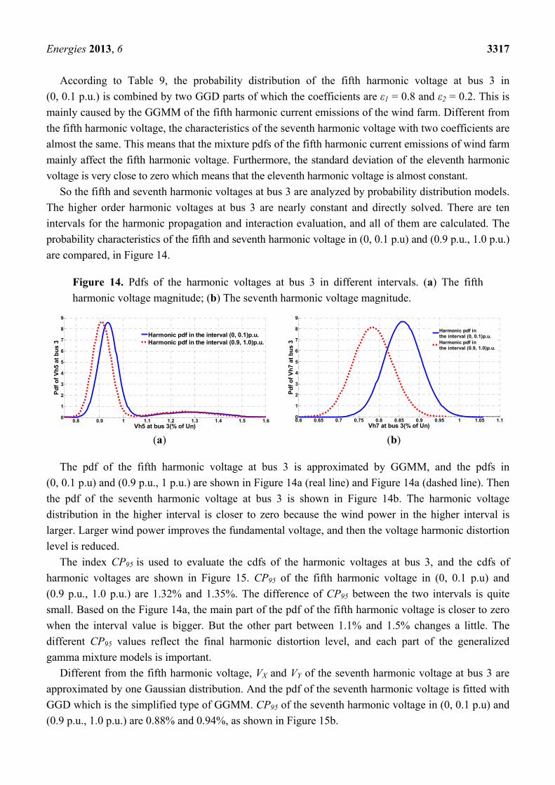
are compared, in Figure 14.
Figure 14. Pdfs of the harmonic voltages at bus 3 in different intervals. (a) The fifth
harmonic voltage magnitude; (b) The seventh harmonic voltage magnitude.
(a) (b)
The pdf of the fifth harmonic voltage at bus 3 is approximated by GGMM, and the pdfs in
(0, 0.1 p.u) and (0.9 p.u., 1 p.u.) are shown in Figure 14a (real line) and Figure 14a (dashed line). Then
the pdf of the seventh harmonic voltage at bus 3 is shown in Figure 14b. The harmonic voltage
distribution in the higher interval is closer to zero because the wind power in the higher interval is
larger. Larger wind power improves the fundamental voltage, and then the voltage harmonic distortion
level is reduced.
The index CP95 is used to evaluate the cdfs of the harmonic voltages at bus 3, and the cdfs of
harmonic voltages are shown in Figure 15. CP95 of the fifth harmonic voltage in (0, 0.1 p.u) and
(0.9 p.u., 1.0 p.u.) are 1.32% and 1.35%. The difference of CP95 between the two intervals is quite
small. Based on the Figure 14a, the main part of the pdf of the fifth harmonic voltage is closer to zero
when the interval value is bigger. But the other part between 1.1% and 1.5% changes a little. The
different CP95 values reflect the final harmonic distortion level, and each part of the generalized
gamma mixture models is important.
Different from the fifth harmonic voltage, VX and VY of the seventh harmonic voltage at bus 3 are
approximated by one Gaussian distribution. And the pdf of the seventh harmonic voltage is fitted with
GGD which is the simplified type of GGMM. CP95 of the seventh harmonic voltage in (0, 0.1 p.u) and
(0.9 p.u., 1.0 p.u.) are 0.88% and 0.94%, as shown in Figure 15b.
0.8 0.9 1 1.1 1.2 1.3 1.4 1.5 1.60
1
2
3
4
5
6
7
8
9
Vh5 at bus 3(% of Un)
Pd
f o
f V
h5
at b
us
3
Harmonic pdf in the interval (0, 0.1)p.u.Harmonic pdf in the interval (0.9, 1.0)p.u.
0.6 0.65 0.7 0.75 0.8 0.85 0.9 0.95 1 1.05 1.10
1
2
3
4
5
6
7
8
9
Vh7 at bus 3(% of Un)
Pd
f o
f V
h7
at b
us
3
Harmonic pdf inthe interval (0, 0.1)p.u.Harmonic pdf inthe interval (0.9, 1.0)p.u.

Energies 2013, 6 3318
Similar to the harmonic analysis in (0, 0.1 p.u) and (0.9 p.u., 1.0 p.u.), pdfs and cdfs of harmonic
voltage at different buses are analyzed. Then the final pdf and cdf of the harmonic voltage are the
linear combination of ten intervals with different weighted coefficients. The comparison of the cdfs of
the harmonic voltages at bus 3 between GGMM and simulation results in PSCAD/EMTDC is shown
in Figure 16.
Figure 15. Cdfs of the harmonic voltages at bus 3 in different intervals. (a) The fifth
harmonic voltage magnitude; (b) The seventh harmonic voltage magnitude.
(a) (b)
Figure 16. Cdfs of the harmonic voltages at bus 3 approximated by GGMM, Gaussian
distribution and simulation results. (a) The fifth harmonic; (b) The seventh harmonic.
(a) (b)
In Figure 16a, CP95 of the fifth harmonic voltage based on the simulation results is 1.29%, and CP95
based on the proposed GGMM combined with the harmonic admittance matrix model is 1.33%. The
difference between the proposed model and simulation result is quite small. Then CP95 of the seventh
harmonic voltage based on the proposed models and simulation results are 0.93% and 0.94%. If the pdf
of the fifth harmonic current is directly approximated by Gaussian distribution, the CP95 values of the
fifth and seventh harmonic voltage are 1.18% and 0.88%. The error is quite big, and it can’t guarantee
the high power quality level. Compared with the Gaussian distribution, the GGMM combined with the
harmonic admittance matrix model simulate and evaluate the propagation and interaction between the
small-scale wind farm and nonlinear loads more accurately.
0.7 0.8 0.9 1 1.1 1.2 1.3 1.4 1.50
0.2
0.4
0.6
0.8
0.951
Vh5 at bus 3(% of Un)
Cd
f o
f V
h5
at b
us
3
Harmonic cdf inthe interval (0, 0.1)p.u.Harmonic cdf inthe interval (0.9, 1.0)p.u.
1.32 1.35
0.6 0.65 0.7 0.75 0.8 0.85 0.9 0.95 1 1.05 1.10
0.2
0.4
0.6
0.8
0.951
Vh7 at bus 3(% of Un)
Cd
f o
f V
h7
at b
us
3
Harmonic cdf inthe interval (0, 0.1)p.u.Harmonic cdf inthe interval (0.9, 1.0)p.u.
0.88 0.94
0.7 0.8 0.9 1 1.1 1.2 1.3 1.4 1.5 1.60
0.2
0.4
0.6
0.8
0.951
Vh5 at bus 3(% of Un)
Cd
f o
f V
h5
at b
us
3
Simulation results base on PSCAD
GGMM combined with harmonicadmittance matrix model
Normal distrib. verify
1.331.291.18
0.6 0.65 0.7 0.75 0.8 0.85 0.9 0.95 1 1.05 1.10
0.2
0.4
0.6
0.8
0.951
Vh7 at bus 3(% of Un)
Cd
f o
f V
h7
at b
us
3
Simulation results base on PSCAD GGMM combined with harmonic admittance matrix model Normal distrib. verify
0.930.88 0.94

Energies 2013, 6 3319
5. Conclusions
The integration of a small-scale wind farm in the distribution grid brings about some challenges to
the system safety and reliability. Non-stationary wind power induces a fluctuating fundamental power
flow, and the non-characteristic harmonic currents of the wind farm interact with the harmonic
emissions of nonlinear loads. In this paper, the fundamental power flow is calculated by the expanding
Newton-Raphson method due to the P – Q(V) characteristic of wind turbines. Generalized gamma
mixture models are proposed to approximate the pdf of harmonic emissions, which are more effective
than general distributions such as the Gaussian, Rayleigh and Weibull ones. Then the voltage harmonic
distortion level of nonlinear loads combined with the wind farm is accurately evaluated by the
harmonic admittance matrix model. The harmonic interaction between the wind farm and nonlinear
loads are calculated by the proposed models. The final results in MATLAB and PSCAD/EMTDC
reveal that the generalized gamma mixture and harmonic admittance matrix models accurately
evaluate the harmonic propagation and interaction between the small-scale wind farm and nonlinear
loads in the distribution grid.
Acknowledgments
This paper is supported by the National High Technology Research and Development Program
of China (2011AA05A101), and the National Basic Research Programs of China (2009CB219702
and 2010CB227206).
Conflict of Interest
The authors declare no conflict of interest.
References
1. Poul, S.; Nicolaos, A.C. Power fluctuations from large wind farms. IEEE Trans. Power Syst.
2007, 22, 958–965.
2. Vittal, E.; Keane, A.; O’Malley, M. Varying Penetration Ratios of Wind Turbine Technologies for
Voltage and Frequency Stability. In Proceeding of the 2008 IEEE Power and Energy Society
General Meeting—Conversion and Delivery of Electrical Energy in the 21st Century, Pittsburgh,
PA, USA, 20–24 July 2008; pp. 1–6.
3. Xie, G.L.; Zhang, B.H. Probabilistic harmonic analysis of wind generators based on generalized
gamma mixture models. Mod. Phys. Lett. B 2013, 27, 1–12.
4. Kasem, A.H.; EI-Saadany, E.F.; EI-Tamaly, H.H. Ramp Rate Control and Voltage Regulation for
Grid Directly Connected Wind Turbines. In Proceedings of the 2008 IEEE Power and Energy
Society General Meeting—Conversion and Delivery of Electrical Energy in the 21st Century,
Pittsburgh, PA, USA, 20–24 July 2008; pp. 31–36.
5. Wu, Y.C.; Ding, M. Simulation study on voltage fluctuations and flicker caused by wind farms.
Power Syst. Technol. 2009, 33, 125–130.
6. Huang, N.E.; Shen, Z.; Steven, R.L. The empirical mode decomposition and the Hilbert spectrum
for nonlinear and non-stationary time series analysis. Proc. R. Soc. 1998, 454, 903–995.

Energies 2013, 6 3320
7. Xu, Y.L.; Asce, M.; Chen, J. Characterizing non-stationary wind speed using empirical mode
decomposition. J. Struct. Eng. 2004, 130, 912–920.
8. Moreno, C.V.; Duarte, H.A.; Garcia, J.U. Propagation of flicker in electric power networks due to
wind energy conversions systems. IEEE Trans. Energy Convers. 2002, 17, 267–272.
9. Bradt, M.; Badrzadeh, B.; Camm, E. Harmonics and Resonance Issues in Wind Power Plants. In
Proceedings of the 2011 IEEE Power and Energy Society General Meeting, San Diego, CA, USA,
24–29 July 2011; pp. 1–8.
10. Novanda, H.; Regulski, P.; Stanojevic, V. Assessment of frequency and harmonic distortions
during wind farm rejection test. IEEE Trans. Sustain. Energy 2013, 4, 698–705.
11. Larose, C.; Gagnon, R.; Homme, P.P. Type-III wind power plant harmonic emissions field
measurements and aggregation guidelines for adequate representation of harmonics. IEEE Trans.
Sustain. Energy 2013, 4, 797–804.
12. Papathanassiou, S.A.; Papadopoulos, M.P. Harmonic analysis in a power system with wind
generation. IEEE Trans. Power Deliv. 2006, 21, 2006–2016.
13. Tentzerakis, S.T.; Papathanassiou, S.A. An investigation of the harmonic emissions of wind
turbines. IEEE Trans. Energy Convers. 2007, 22, 150–158.
14. Bonner, A.; Grebe, T.; Hopkins, L. Modeling and simulation of the propagation of harmonics in
electric power networks. Part I: Concepts, models and simulation techniques. IEEE Trans. Power
Deliv. 1996, 11, 452–465.
15. Sun, Y.Y.; Zhang, G.B.; Xu, W. A harmonically coupled admittance matrix model for AC/DC
converters. IEEE Trans. Power Syst. 2007, 22, 1574–1582.
16. Liang, X.D.; Luy, Y.; Don, O.K. Investigation of Input Harmonic Distortions of Variable
Frequency Drives. In Proceedings of the Industrial & Commercial Power Systems Technical
Conference (ICPS 2007), Edmonton, Canada, 6–11 May 2007; pp. 1–11.
17. Verma, V.; Singh, B.; Chandra, A. Power conditioner for variable-frequency drives in offshore oil
fields. IEEE Trans. Ind. Appl. 2010, 46, 731–739.
18. Sharma, V.; Fleming, R.J.; Niekamp, L. An iterative approach for analysis of harmonic
penetration in the power transmission networks. IEEE Trans. Power Deliv. 1991, 6, 1698–1706.
19. Hu, W.H.; Wang, W.; Wang, Y.L.; Xiao, H.B. Power flow analysis in electrical power system
including wind farms. North China Electr. Power 2006, 10, 12–15.
20. Li, Y.; Luo, Y.L.; Zhang, B.H.; Mao, C.X. A Modified Newton-Raphson Power Flow Method
Considering Wind Power. In Proceedings of the 2011 Asia-Pacific Power and Energy Engineering
Conference (APPEEC), Wuhan, China, 25–28 March 2011; pp. 1–5.
21. Feijoo, A.E.; Cidras, J. Modeling of wind farms in the load flow analysis. IEEE Trans. Power Syst.
2000, 15, 110–115.
22. Miller, N.W.; Sanchez-Gasca, J.J.; Price, W.W. Dynamic Modeling of GE 1.5 and 3.6 MW Wind
Turbine-Generators for Stability Simulations. In Proceedings of the IEEE Power Engineering
Society General Meeting, Toronto, Canada, 13–17 July 2003; Volume 3, pp. 1977–1983.
23. Lindholm, M.; Ramussen, T.W. Harmonic Analysis of Doubly Fed Induction Generators. In
Proceedings of the Fifth International Conference on Power Electronics and Drive Systems
(PEDS 2003), Singapore, 17–20 November 2003;Volume 2, pp. 837–841.

Energies 2013, 6 3321
24. Zhong, W.; Sun, Y.Z.; Li, G.J.; Li, Z.G. Stator current harmonics analysis of doubly-fed induction
generator. Electr. Power Autom. Equip. 2010, 30, 1–5.
25. Fan, L.L.; Yuvarajan, S.; Kavasseri, R. Harmonic analysis of a DFIG for a wind energy
conversion system. IEEE Trans. Energy Convers. 2010, 25, 181–189.
26. King, R.; Ekanayake, J.B. Harmonic Modelling of Offshore Wind Farms. In Proceedings of the
2010 IEEE Power and Energy Society General Meeting, Minneapolis, MN, USA, 25–29 July
2010; pp. 1–6.
27. Schostan, S.; Dettmann, K.D.; Thanh, T.D.; Schulz, D. Harmonic Propagation in a Doubly Fed
Induction Generator of a Wind Energy Converter. In Proceedings of the Compatibility and Power
Electronics (CPE 2009), Badajoz, Spain, 20–22 May 2009; pp. 101–108.
28. Kiani, M.; Lee, W.J. Effects of voltage unbalance and system harmonics on the performance of
doubly fed induction wind generators. IEEE Trans. Ind. Appl. 2010, 46, 562–568.
29. Francesco, C.D.; Matteo, F.I.; Roberto, P. An observer for sensorless DFIM drives based on the
natural fifth harmonic of the line voltage, without stator current measurement. IEEE Trans. Ind.
Electr. 2013, 60, 4301–4309.
30. Liu, C.J.; Blaabjerg, F.; Chen, W.J. Stator current harmonic control with resonant controller for
doubly fed induction generator. IEEE Trans. Power Electr. 2012, 27, 3207–3220.
31. Sainz, L.; Mesas, J.J.; Teodorescu, R. Deterministic and stochastic study of wind farm harmonic
currents. IEEE Trans. Energy Convers. 2010, 25, 1071–1081.
32. Cavallini, A.; Langella, R.; Testa, A. Gaussian Modeling of Harmonic Vectors in Power Systems.
In Proceedings of the 8th International Conference on Harmonics and Quality of Power, Athens,
Greece, 14–16 October 1998; pp. 1010–1017.
33. Baghzouz, Y.; Burch, R.F.; Capasso, A. Time-varying harmonics: II-harmonic summation and
propagation. IEEE Trans. Power Syst. 2002, 17, 279–285.
34. Wilson, R. Multiresolution Gaussian Mixture Models: Theory and Application; Research Report
RR404; Department of Computer Science, University of Warwick: Warwickshire, UK, 1999.
35. Zhao, Y.X.; Zhuang, X.H.; Ting, J.S. Gaussian mixture density modeling of non-gaussian source
for autoregressive process. IEEE Trans. Signal. Proc. 1995, 43, 894–903.
36. Moon, T. The expectation-maximization algorithm. IEEE Signal. Proc. Mag. 1996, 13, 47–60.
37. Lu, X.; Rogers, C.; Peng, F.Z. A Double Fourier Analysis Development of THD for PWM
Inverters: A Theoretical Method for Motor Loss Minimization. In Proceedings of the 2010 IEEE
Energy Conversion Congress and Exposition (ECCE), Atlanta, GA, USA, 12–16 September 2010;
pp. 1505–1510.
38. Fioretto, M.; Raimondo, G.; Rubino, L. Evaluation of Current Harmonic Distortion in Wind Farm
Application Based on Synchronous Active Front End Converters. In Proceedings of the IEEE
African Conference (AFRICON 2011), Livingstone, Zambia, 13–15 September 2011; pp. 1–6.
39. Holmes, D.G.; Lipo, T.A. Pulse Width Modulation for Power Converters: Principles and Practice;
IEEE Press Series on Power Engineering; John Wiley & Sons: Manhattan, NY, USA, 2003;
pp. 140–144.

Energies 2013, 6 3322
40. Papathanassiou, S.; Hatziargyriou, N.; Strunz, K. A Benchmark Low Voltage Microgrid Network.
In Proceedings of the International Conference on Large High Voltage Electric System (CIGRE)
Symposium: Power Systems with Dispersed Generation, Athens, Greece, 13–16 April 2005;
pp. 1–8.
41. Rudion, K.; Styczynski, Z.A.; Hatziargyriou, N. Development of Benchmarks for Low and
Medium Voltage Distribution Networks with High Penetration of Dispersed Generation. In
Proceedings of the 3rd International Symposium on Modem Electric Power System, Wroclaw,
Poland, 6–8 September 2006; pp. 1–7.
42. Liang, S.; Hu, Q.H.; Lee, W.J. A Survey of Harmonic Emissions of a Commercial Operated Wind
Farm. In Proceedings of the IEEE Industrial and Commercial Power Systems Technical
Conference, Tallahassee, FL, USA, 9–13 May 2010; pp. 1–8.
© 2013 by the authors; licensee MDPI, Basel, Switzerland. This article is an open access
article distributed under the terms and conditions of the Creative Commons Attribution license
(http://creativecommons.org/licenses/by/3.0/).
Recommended