ELECTROMAGNETIC SENSORS FOR MEASUREMENTS ON

ELECTRIC POWER TRANSMISSION LINES

By

ZHI LI

A dissertation submitted in partial fulfillment of

the requirements for the degree of

DOCTOR OF PHILOSOPHY

WASHINGTON STATE UNIVERSITY

School of Electrical Engineering and Computer Science

AUGUST 2011

ii

To the Faculty of Washington State University:

The members of the Committee appointed to examine the

dissertation of ZHI LI find it satisfactory and recommend that it be accepted.

___________________________________

Robert G. Olsen, Ph.D., Chair

___________________________________

Patrick D. Pedrow, Ph.D.

___________________________________

Mani V. Venkatasubramanian, Ph.D.

iii

ACKNOWLEDGMENT

I would like to thank my advisor Dr. Robert G. Olsen for his endless help during

my stay in Pullman. He ignited my interest in the research on electromagnetics for

power transmission lines. His patient and inspiring guidance always brought me back

on the right track when I got lost in my research. Without his help and encourage, this

dissertation would not have been possible. Also thanks to his mentoring of my life

under the American culture background. I would like to thank my committee, Dr.

Patrick D. Pedrow and Dr. Mani V. Venkatasubramanian for the helpful inputs for my

research and career pursuits. Special thanks to, but not limit to, Dr. Anjan Bose, Dr.

John B. Schneider, and Dr. Aleksandar D. Dimitrovski for help in my research and

graduate curriculum.

I would also like to thank my parents and my family for their continuous support

and unconditional love, which have always been the source of my courage. Deepest

appreciation also to my friends, whose support and encourage have helped shape this

amazing journey in my life.

Thanks to Xiaojing for holding my hand, with love.

iv

ELECTROMAGNETIC SENSORS FOR MEASUREMENTS ON

ELECTRIC POWER TRANSMISSION LINES

Abstract

by Zhi Li, Ph.D.

Washington State University

August 2011

Chair: Robert G. Olsen

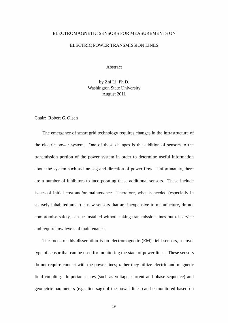
The emergence of smart grid technology requires changes in the infrastructure of

the electric power system. One of these changes is the addition of sensors to the

transmission portion of the power system in order to determine useful information

about the system such as line sag and direction of power flow. Unfortunately, there

are a number of inhibitors to incorporating these additional sensors. These include

issues of initial cost and/or maintenance. Therefore, what is needed (especially in

sparsely inhabited areas) is new sensors that are inexpensive to manufacture, do not

compromise safety, can be installed without taking transmission lines out of service

and require low levels of maintenance.

The focus of this dissertation is on electromagnetic (EM) field sensors, a novel

type of sensor that can be used for monitoring the state of power lines. These sensors

do not require contact with the power lines; rather they utilize electric and magnetic

field coupling. Important states (such as voltage, current and phase sequence) and

geometric parameters (e.g., line sag) of the power lines can be monitored based on

v

inherent correlations between those variables and the electromagnetic fields produced

by the power lines. While similar sensors have been available for many years, the

unique feature of the sensors discussed here is that they utilize the relative phase of

the EM fields in the vicinity of the line to provide significantly better sensitivity than

has been previously available. In addition, they are inexpensive, easy to install with

live working techniques and require only a low level of maintenance.

Three types of sensors, point probes, and perpendicular and parallel distributed

sensors will be studied using basic reciprocity theory and developed to the point of

application. Several field experiments were conducted for validation. Finally,

potential applications of the sensors for monitoring power lines are explored.

vi

TABLE OF CONTENTS

Page

ACKNOWLEDGMENT .......................................................................................... III

ABSTRACT ............................................................................................................... IV

TABLE OF CONTENTS .......................................................................................... VI

LIST OF FIGURES .................................................................................................. IX

LIST OF TABLES .................................................................................................. XIII

CHAPTER 1 INTRODUCTION .............................................................................. 1

1.1 ELECTROMAGNETIC SENSORS FOR TRANSMISSION LINES ...................................... 4

1.2 EM FIELDS DUE TO POWER TRANSMISSION LINES ................................................. 7

CHAPTER 2 POINT PROBES .............................................................................. 15

2.1 INTRODUCTION.................................................................................................... 15

2.2 GENERAL THEORY OF POINT PROBES.................................................................... 17

2.3 APPLICATIONS OF POINT PROBE ........................................................................... 23

2.3.1 Power line voltage monitoring .................................................................... 23

2.3.2 Sag monitoring ............................................................................................ 26

2.3.3 Negative/Zero sequence voltage detection ................................................. 28

2.4 LAB TESTS AND FIELD EXPERIMENTS OF POINT PROBE ........................................ 35

2.4.1 Single-phase, single-probe lab test ............................................................ 35

vii

2.4.2 Single-phase, two-probe lab test ................................................................ 37

2.4.3 Field experiments ........................................................................................ 38

CHAPTER 3 GENERAL THEORY OF LINEAR SENSORS ............................ 44

3.1 APPROACH BY RECIPROCITY THEOREM ................................................................ 44

3.1.1 Reciprocity theorem for general electromagnetic case ............................... 46

3.1.2 Two situations for implementing reciprocity theorem ................................ 47

3.1.3 Implementing reciprocity theorem .............................................................. 49

3.1.4 Solutions to the horizontal sensor case ....................................................... 54

3.2 APPROACH BY MODEL OF PER-UNIT-LENGTH VOLTAGE AND CURRENT SOURCES .. 56

3.3 RELATIONSHIP BETWEEN THE TWO APPROACHES ................................................. 61

CHAPTER 4 PERPENDICULAR LINEAR SENSORS ..................................... 66

4.1 MODEL AND THEORIES........................................................................................ 67

4.2 SAG MONITORING BY PERPENDICULAR LINEAR SENSOR ...................................... 75

4.2.1 Power line models and parameters ............................................................ 75

4.2.2 Effect of setting of Z1 and Z2 ...................................................................... 77

4.2.3 Effect of sensor length ............................................................................... 80

4.2.4 Effect of sensor height ............................................................................... 84

4.2.5 Discussion on characteristic parameters of the sensor wire....................... 85

4.3 NEGATIVE SEQUENCE MODE DETECTION BY PERPENDICULAR LINEAR SENSOR .... 88

CHAPTER 5 PARALLEL LINEAR SENSORS ................................................... 97

5.1 DIRECTIONAL COUPLER ....................................................................................... 98

viii

5.2 FIELD EXPERIMENTS FOR DIRECTIONAL COUPLER.............................................. 106

5.2.1 Objective and model ................................................................................. 106

5.2.2 Settings and preparations of experiment ................................................... 109

5.2.3 Results and analysis .................................................................................. 121

CHAPTER 6 LOW FREQUENCY DIPOLE IN THREE-LAYER MEDIUM .. 133

6.1 MODEL ............................................................................................................. 134

6.2 FORMULATIONS BY SOMMERFELD INTEGRALS .................................................. 137

6.3 UP-OVER-AND-DOWN INTERPRETATION OF THE FIELD PROPAGATIONS .............. 148

6.3.1 Simplification of the integral of Iz1 and Iy1 ............................................... 151

6.3.2 Approximations for E and H fields .......................................................... 162

6.3.3 Up-over-and-down interpretation of wave propagation near interface ..... 164

REFERENCES ......................................................................................................... 171

ix

LIST OF FIGURES

Fig. 1-1 Structure of a typical power system ................................................................ 2

Fig. 1-2 An EM sensor made of styrofoam sphere covered by aluminum foils ........... 5

Fig. 1-3 Patterns of electric and magnetic field flux of a power transmission line ...... 8

Fig. 1-4 Fluorescent tubes lighted by EM field surrounding power lines .................... 9

Fig. 1-5 Simplified model for transmission line above half-space of earth ................ 10

Fig. 2-1 A general model of the point probe. .............................................................. 17

Fig. 2-2 Two states of the point probe for applying the reciprocity theorem ............. 18

Fig. 2-3 Thevenin equivalent circuit for the point probe model ................................. 21

Fig. 2-4 Configuration of a 230kV, three phase, horizontal transmission line ........... 24

Fig. 2-5 Space potential profiles for positive sequence voltage ................................. 24

Fig. 2-6 Single probe placed under the three-phase power line .................................. 25

Fig. 2-7 Applied voltage on the power line vs. induced current in point probe.......... 26

Fig. 2-8 Line sag vs. induced current in point probe. ................................................. 27

Fig. 2-9 Space potential profiles for negative sequence power line voltage .............. 29

Fig. 2-10 Two probes designed to detect negative sequence component ................... 30

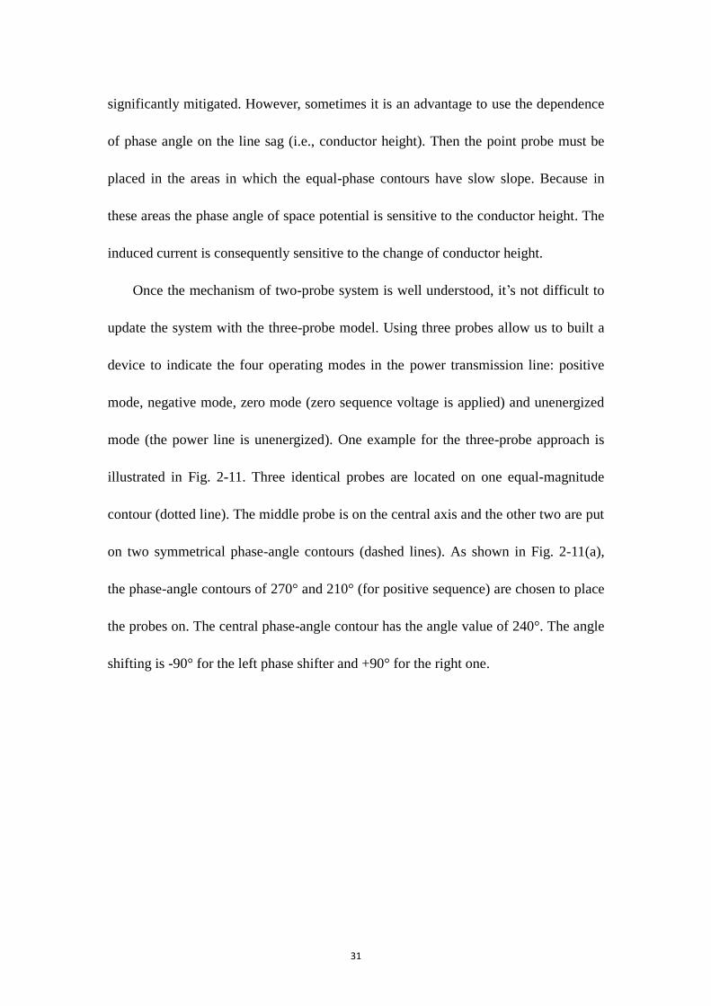
Fig. 2-11 Design of a three-probe device used as a four-mode indicator ................... 32

Fig. 2-12 Design of a negative-to-positive ratio measurement device ....................... 33

Fig. 2-13 Single-phase, single-probe lab test .............................................................. 36

Fig. 2-14 Space potential meter .................................................................................. 36

x

Fig. 2-15 Single-phase, two-probe lab test ................................................................. 37

Fig. 2-16 The site of the field experiment for point probe .......................................... 38

Fig. 2-17 Positive sequence space potential profiles of the testing power line .......... 39

Fig. 2-18 Settings for the field experiment ................................................................. 40

Fig. 2-19 Probe currents of the field experiments....................................................... 42

Fig. 2-20 Total current of the field experiments ......................................................... 42

Fig. 3-1 A general model of the linear sensor ............................................................. 45

Fig. 3-2 Special case for reciprocity theorem: sources reduces to line currents ......... 47

Fig. 3-3 Two situations for implementing reciprocity theorem .................................. 48

Fig. 3-4 Thevenin‘s equivalent circuit for the linear sensor system ........................... 53

Fig. 3-5 Model of the horizontal lossy wire sensor .................................................... 54

Fig. 3-6 Model of a horizontal lossy linear sensor over perfect conductor ground .... 57

Fig. 3-7 Replacing the external excitation with per-unit-length induced sources ...... 57

Fig. 3-8 The sensor driven by only one set of the per-unit-length sources ................. 58

Fig. 3-9 Equivalent circuit of the model driven by only one pair of sources ............. 59

Fig. 4-1 Circuit loop of the perpendicular linear sensor and magnetic flux ............... 66

Fig. 4-2 Model of a perpendicular linear sensor system. ............................................ 68

Fig. 4-3 A perpendicular linear sensor reduces to point probe ................................... 73

Fig. 4-4 Geometries of the perpendicular wire sensor ................................................ 75

Fig. 4-5 Magnitude of the induced current on the sensor when Z1 = Z2 = 100Ω ........ 78

Fig. 4-6 Phase angle of the induced current on the sensor when Z1 = Z2 = 100Ω ...... 79

Fig. 4-7 Magnitude of the induced current when Z1 = 100Ω and Z2 = ∞ ................... 80

xi

Fig. 4-8 Induced current at x = - L/2 vs. sensor length (Z1 = 100Ω, Z2 = 100Ω) ......... 81

Fig. 4-9 Integration of space potential alone over the sensor wire. ............................ 82

Fig. 4-10 Induced current at x = - L/2 vs. sensor length (Z1 = 100Ω, Z2 = ∞) ............ 83

Fig. 4-11 Sensor length vs. line sag for Model A (Z1 = 100Ω and Z2 = 100Ω) ........... 85

Fig. 4-12 Induced current at x = - L/2 vs. sensor length for different rw ..................... 86

Fig. 4-13 Induced current at x = - L/2 vs. sensor length for different cw .................... 87

Fig. 4-14 Using perpendicular linear sensors to detect negative sequence voltage .... 89

Fig. 4-15 Magnitude of I1 and I2: (a) positive and (b) negative mode ........................ 90

Fig. 4-16 Phase angle of I1 and I2: (a) positive and (b) negative mode ...................... 90

Fig. 4-17 Design of perpendicular linear sensors to detect negative mode ................ 91

Fig. 4-18 Magnitude of Itot for different modes after ±30º phase shifting .................. 92

Fig. 4-19 Move the two probes away from the center by 0.3m .................................. 93

Fig. 4-20 Magnitude of total current when the probes are moved by 0.3 m ............... 94

Fig. 4-21 Magnitude of total current for different modes of voltage in Model B ....... 95

Fig. 5-1 Model of a horizontal parallel sensor ............................................................ 97

Fig. 5-2 Polarities of (a) traveling wave; (b), (c) capacitive and inductive current. . 101

Fig. 5-3 Settings of the field experiment for directional couplers ............................ 107

Fig. 5-4 Resistor and capacitor connected in series and parallel .............................. 108

Fig. 5-5 Experiment site and settings of the experiments for directional couplers. .. 112

Fig. 5-6 Measurements of Ey compared to the calculated values. ............................ 113

Fig. 5-7 Copper wire and pipes used for sensor and grounding rods ....................... 114

Fig. 5-8 Fall of Potential method for earth resistance measurement. ....................... 117

xii

Fig. 5-9 Calculations of magnitude and angle of ΓTL. ............................................... 119

Fig. 5-10 Three positions to place the sensor............................................................ 120

Fig. 5-11 Measured I1 and I2 (on May 4th

) vs. simulations when x = - 6m. .............. 123

Fig. 5-12 Measured I1 and I2 (on May 4th

) vs. simulations when x = 0. ................... 123

Fig. 5-13 Measured I1 and I2 (on May 4th

) vs. simulations when x = + 6m. ............. 124

Fig. 5-14 Measured I1 and I2 (on May 25th

) vs. simulations when x = - 6m. ............ 126

Fig. 5-15 Equal magnitude contours of I1 over the C-R grid .................................... 127

Fig. 5-16 Calculated I1 and I2 for different values of ΓTL (x = - 6m) ........................ 129

Fig. 5-17 Equal magnitude contours of I1 over the C-R grid for different ΓTL ......... 130

Fig. 6-1 Model of three-layer medium with a HED buried in the middle layer ....... 134

Fig. 6-2 Integration intervals for the composite Simpson‘s rule ............................... 144

Fig. 6-3 Comparisons between fields by integration and the quasi-static fields ...... 147

Fig. 6-4 Model of a HED buried in lower half space of conducting medium #1 ..... 148

Fig. 6-5 Illustration of the up-over-and-down path. ................................................. 149

Fig. 6-6 Deformation of the integral contour for the integration of Iz1 ..................... 153

Fig. 6-7 Total integration, integration along branch cut of k0, and the residue ......... 154

Fig. 6-8 Exact integral of Iz1 vs. approximation: (a) magnitude, (b) phase angle. .... 159

Fig. 6-9 Exact integral of Iy1 vs. approximation: (a) magnitude, (b) phase angle. .... 162

Fig. 6-10 Exact reflected field E1yr vs. its approximation (6.57b), φ = π. ................. 164

Fig. 6-11 (a) The static charge dipole replacing the HED and (b) its image. ........... 166

Fig. 6-12 Equivalent surface charges qs on the interface (z = 0 plane). .................... 168

Fig. 6-13 Equivalent charge (a) nonuniform distribution (b) dipole moment. ......... 169

xiii

LIST OF TABLES

Table 2-1 Four sequence modes and their corresponding current statuses ................. 32

Table 2-2 Results for computer simulation ................................................................. 35

Table 2-3 Results of single-phase, single-probe lab test ............................................. 36

Table 2-4 Results of single-phase, two-probe test ...................................................... 38

Table 2-5 Parameters of the two-probe device ........................................................... 40

Table 2-6 Original data of induced current ................................................................. 41

Table 4-1 Power line configures and sensor parameters ............................................. 76

Table 4-2 Designs of the perpendicular linear sensor for sag monitoring ................... 88

Table 5-1 Information of the tested power transmission line ................................... 113

Table 5-2 Geometries of the sensor and grounding system ...................................... 115

Table 5-3 Measurements of earth resistance Rg of grounding system ...................... 117

Table 5-4 Some calculated ΓTL for Ip = 221A and 225A ........................................... 120

Table 5-5 Calculated Z1, resistances and capacitances causing the null ................... 122

Table 6-1 Models for the eight cases of different dipole sources ............................. 136

Table 6-2 Parameters used in the simulations for the numerical validation ............. 143

xiv

To my mother and father

1

CHAPTER 1

INTRODUCTION

Since the commercial electric power system started to serve our society in late 1800‘s,

the transmission line has become a significant part of the system. After more than 100

years‘ development, the modern power system is much more advanced than its

ancestor. When the first transmission line in North America was built in 1889, it was

only about 13 miles long and delivered power from Willamette Falls in Oregon City

to downtown Portland at a voltage of 4000 V [1]. Nowadays, high voltage

transmission lines can convey huge amounts of power over hundreds or even

thousands of miles from the generation center to the consumer center. Many kinds of

devices and sensors are installed to monitor the flow of power through the

transmission line and ensure that the power system is operated efficiently as well as

reliably. These sensors also play important roles in providing the protection for the

power system during abnormal operations and faults. The sensor itself is a testing

field for the state-of-art technologies. Many high-tech methods or concepts, such as

robotics, GPS technique, and radar imaging, have been adapted in developing the

sensors and significantly improve the performance of the sensor network for the

power system.

With all these efforts, however, power engineers still cannot help asking this

question: Is it enough to operate a reliable, smart as well as economically efficient

electric power system? Obviously, the answer is No. Here the focus is on the

transmission line system. Fig. 1-1 shows the basic structure of a power system,

2

containing the subsystem of, from left to right, power generation, transmission, and

distribution.

Fig. 1-1 Structure of a typical power system, usually not enough sensors are installed

for the transmission lines (Image source:

http://www.ferc.gov/industries/electric/indus-act/reliability/blackout/ch1-3.pdf)

As well known, the traditional sensors such as potential transformers (PT‘s) and

current transformers (CT‘s) are usually installed in the substations. However, on the

power transmission lines (shown in the dashed square in Fig. 1-1), which are often

spread out over wide areas, an inadequate number of sensors have been deployed.

There is useful information, such as line sag, direction of power flow, and

environmental electromagnetic field, that are not well monitored in these areas. In the

Department of Energy‘s ―Five-year program plan for fiscal years 2008 to 2012 for

electric transmission and distribution programs‖ [2], it is proposed to deploy at least

100 transmission-level sensors by 2009 to enhance the capability of real-time

monitoring of the power system. The ―transmission-level sensors‖ in this report

include phasor measurement units (PMUs), intelligent electronic devices (IEDs) and

sag monitors. It is reported that prior to 2009, more than 200 PMUs have been

installed in the North American power system interconnection with more to come [3].

3

Obviously, compared to the scale of the power system, several hundred sensors are far

from enough to significantly improve the sensor networks for the transmission system

of the power grid. It is cost which limits the number of the sensors to be installed.

Those sensors are usually very expensive and require many of labor hours for

installation and maintenance.

Moreover, it has been the common understanding that the ‗Smart Grid‘ will be the

future of the electric power system. To build a smarter power system requires reform

of the infrastructure, for which the sensor network is an important part. Instead of

changing all the existing grid at once, the better and more feasible idea is to gradually

replace the old components with new technologies and, at the same time, improve the

ability to access and monitor the conditions of the rest of the grid components so that

it operates more efficiently and reliably [4], [5]. This brings technical and economic

challenges to advancing the sensor networks. The types of sensors chosen for the new

sensor networks should have the following characteristics:

Capable of picking up the desired signals under complicated background

conditions, accurately and reliably;

Inexpensive for manufacture and maintenance;

Easy and safe to install.

Especially for power transmission lines, which are geographically widely spread

in sparsely inhabited areas, the sensors should be inexpensive, easy to install with live

line work, and require a very low level of maintenance. Given these characteristics,

the sensors can be deployed in large numbers to significantly increase the density of

4

the sensor networks for transmission system of the power grid.

New sensors and sensing technologies have been developed for transmission lines.

For example, a conductor temperature sensor and a connector condition sensor are

introduced in [4]. The first sensor measures the conductor temperature and current

directly. The second one monitors the condition of the conductor connectors by

measuring temperature or resistance of the connector. Sensors based on fiber-Optic

and infrared imaging techniques have been used for measuring the leakage current

and contamination level of insulators on transmission lines [6] – [9]. [10] shows the

automatic visual power line inspection conducted by a robot equipped with cameras.

Real-time sag monitoring of the power line conductors is important for the dynamic

rating of power lines; they detect dangerous increases in line sag due to overheating or

ice covering, and prevent line to ground short circuit faults. Power line sag can be

measured by several types of sensors or techniques, such as satellite imaging [11],

power-line carrier (PLC) signal analysis [12], global positioning system (GPS) sensor

[13], [14], mechanical tension sensor [15], or space potential probe [16], [17].

1.1 Electromagnetic sensors for transmission lines

The sensors to be studied in this dissertation are ones that achieve the desired

measurements by means of electromagnetic (EM) coupling with the fields produced

by power transmission lines. Basically, these sensors (will be called the ‗EM sensors‘

in the dissertation) are the receiving antennas that work with the EM fields due to the

power transmission lines. The first pair of transmitting and receiving antennas,

5

employed by Hertz in 1887, had a very simple design [18]. The receiving antenna was

simply formed by a circular loop of wire with a tiny gap. The EM sensors introduced

here inherit the characteristic of simplicity from Hertz‘s antennas. It is not necessary

to have complex structures, which means the manufacturing costs are low. In fact, a

simple conducting sphere or a loop of conductor can be used as an EM sensor for

acquisition of useful information from power lines. An EM sensor made of a

styrofoam sphere covered by aluminum foil and the supporting frames made of PVC

pipes are shown in Fig. 1-2. When grounded through an ammeter, this sensor can be

used to measure the space potential, i.e., the capacitive coupling, due to the power

lines. Details of this kind of sensor will be introduced in Chapter 2.

Fig. 1-2 An EM sensor made of styrofoam sphere covered by aluminum foils and the

PVC supporting frame

Since the EM sensors work with the EM fields due to the power line, the

measurements can be conducted in a non-contact manner, which means that the

6

sensors don‘t have to have physical contact with the power line conductors and can be

placed relatively far away from the high voltage parts. This avoids concerns about

high voltage insulation, and further, reduces the manufacture costs of the sensor

system. The EM sensors with the corresponding meters, data storage, and even

communication system still cost much less than many other kinds of sensors in use,

such as PTs, CTs, or GPS sag monitors. Benefiting from the non-contact

characteristics of the EM sensor, the installation becomes simple and inexpensive.

Further, the power line doesn‘t need to be shut down when the EM sensor is installed

because it is placed far enough (usually on the ground) from the power line conductor.

Usually, the result of the electromagnetic coupling from power lines are the

induced current or voltage on the EM sensors. The EM fields due to power lines are

determined by the variables such as line voltage, current, and line configuration,

which are all very useful pieces of information about the operation and control of the

power system. Inherent connections are consequently built between the induced

current or voltage and the states or parameters of the power lines. Then, these pieces

of information about the power lines can be derived, i.e., indirectly measured, by the

measurements from the EM sensor. This is the basic mechanism how the EM sensors

work. Therefore, the EM sensors have the ability to accomplish many tasks now done

by the traditional sensors. Different from the traditional measurements of EM fields

for which only the magnitudes of the fields are measured, the utilization of the phase

angle of the fields gives more strength to the EM sensors discussed here, if properly

designed. In addition, the EM sensors, with simple design and structure, require very

7

low level of maintenance, which results in that the sensors can be installed in various

areas, including those far away from the population centers. All these advantages

imply that the EM sensors have the potential to be deployed in large number in the

power transmission system and make the family of EM sensors a good choice for

advancing the sensor network for power transmission lines.

The designs of EM sensors vary between different applications. Each kind of the

EM sensor is designed to measure the desired variables or states. The types of EM

sensors to be studied in this dissertation are the point probes (capacitive coupling

sensors), perpendicular linear sensors (capacitive coupling sensors), and parallel

linear sensors (capacitive and inductive coupling sensors).

1.2 EM fields due to power transmission lines

As is well known, in the vicinity of an energized power transmission line there exist

electromagnetic fields. Though it is usually difficult (if not impossible) for humans to

directly perceive the existence of these fields, well-designed sensors can help to detect

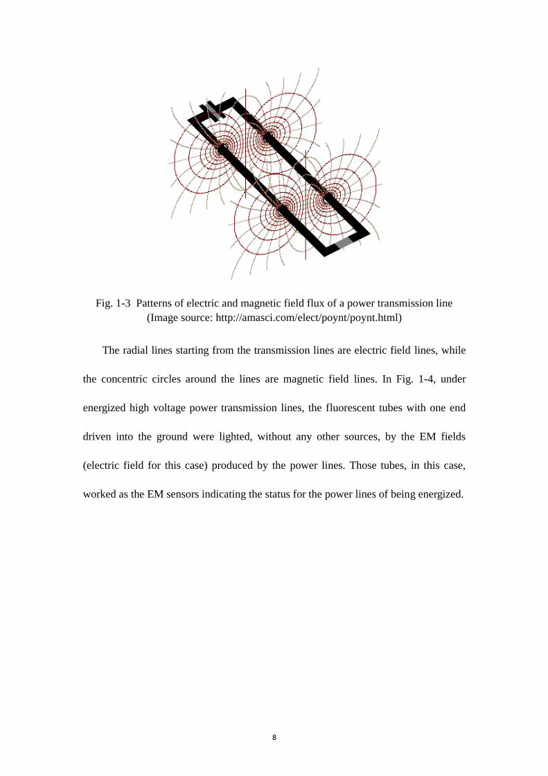
and measure them. Fig. 1-3 illustrates the patterns of the transverse electric and

magnetic field fluxes of a two-conductor transmission line.

8

Fig. 1-3 Patterns of electric and magnetic field flux of a power transmission line

(Image source: http://amasci.com/elect/poynt/poynt.html)

The radial lines starting from the transmission lines are electric field lines, while

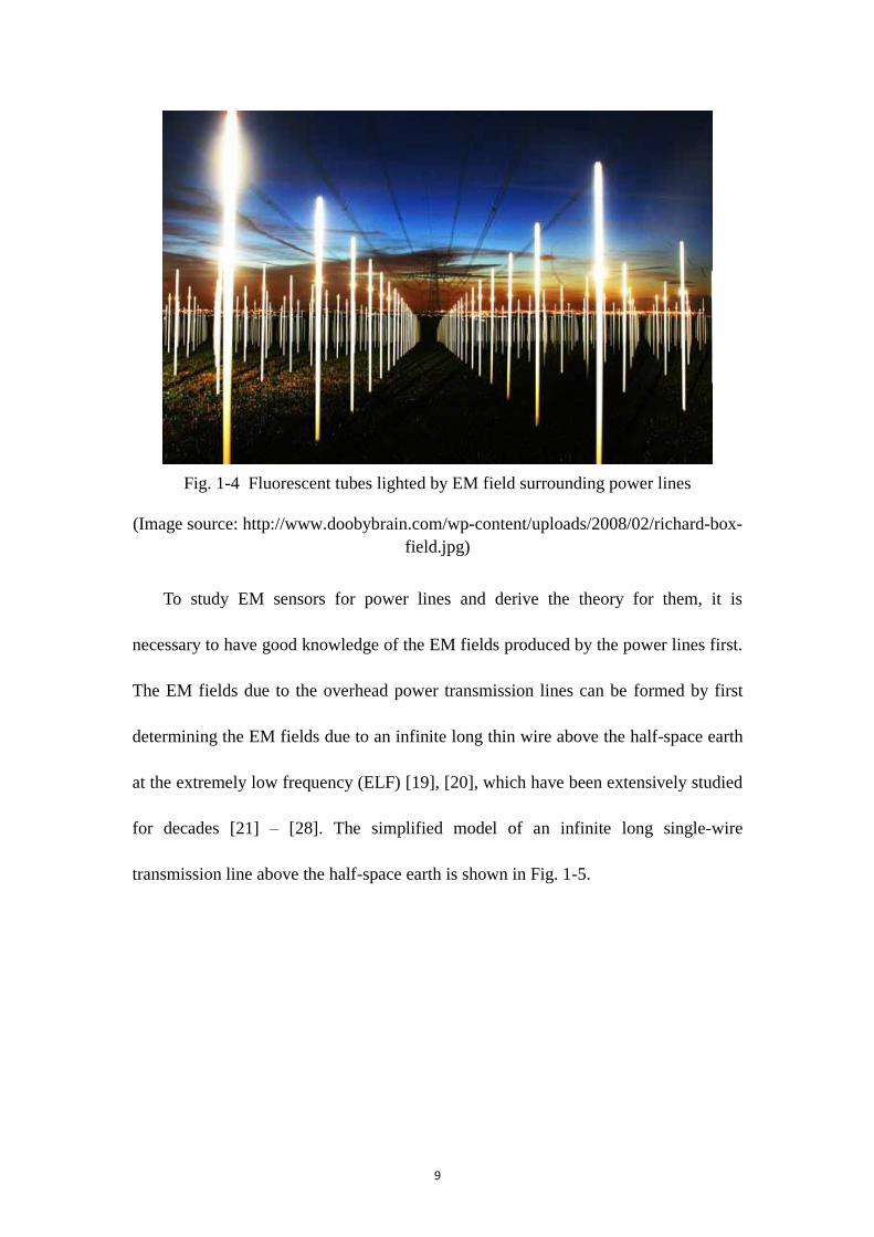
the concentric circles around the lines are magnetic field lines. In Fig. 1-4, under

energized high voltage power transmission lines, the fluorescent tubes with one end

driven into the ground were lighted, without any other sources, by the EM fields

(electric field for this case) produced by the power lines. Those tubes, in this case,

worked as the EM sensors indicating the status for the power lines of being energized.

9

Fig. 1-4 Fluorescent tubes lighted by EM field surrounding power lines

(Image source: http://www.doobybrain.com/wp-content/uploads/2008/02/richard-box-

field.jpg)

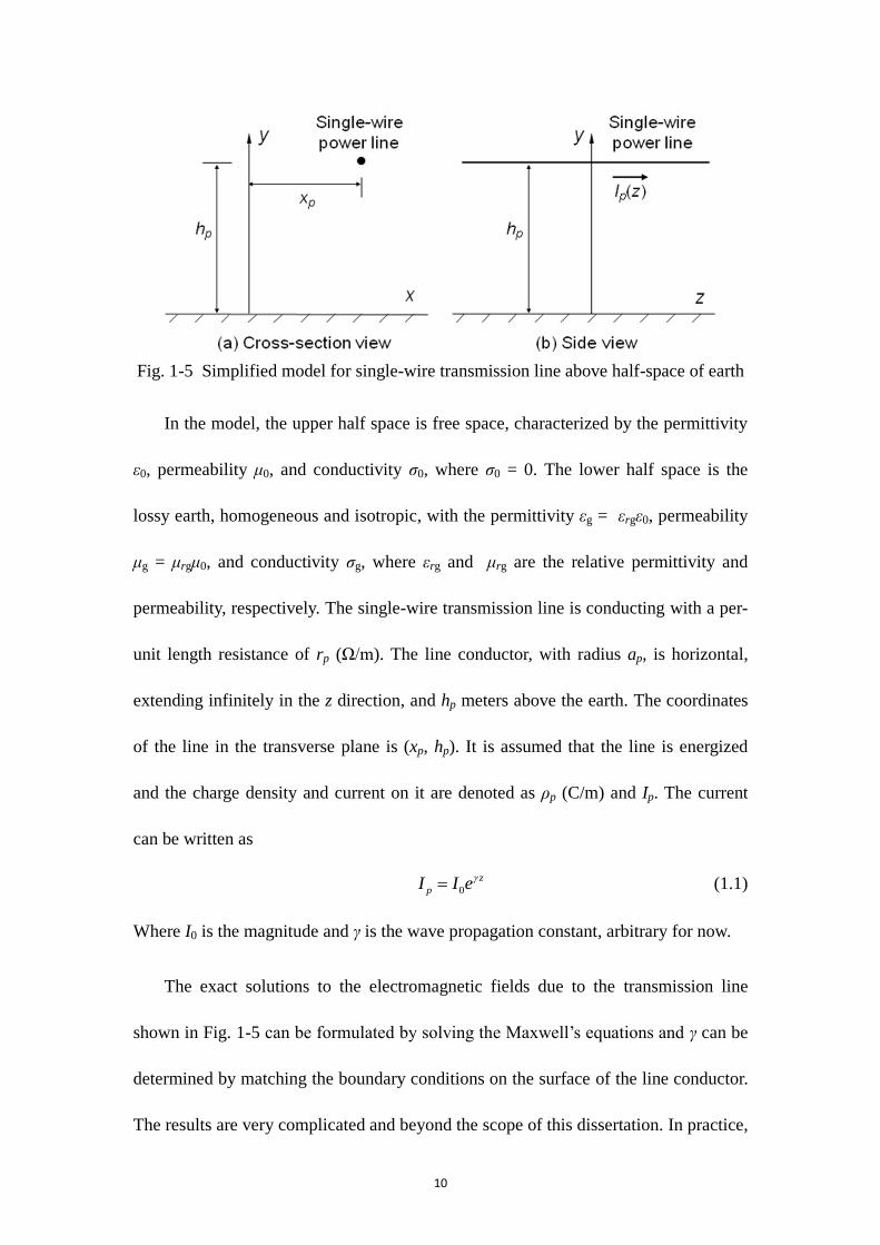
To study EM sensors for power lines and derive the theory for them, it is

necessary to have good knowledge of the EM fields produced by the power lines first.

The EM fields due to the overhead power transmission lines can be formed by first

determining the EM fields due to an infinite long thin wire above the half-space earth

at the extremely low frequency (ELF) [19], [20], which have been extensively studied

for decades [21] – [28]. The simplified model of an infinite long single-wire

transmission line above the half-space earth is shown in Fig. 1-5.

10

Fig. 1-5 Simplified model for single-wire transmission line above half-space of earth

In the model, the upper half space is free space, characterized by the permittivity

ε0, permeability μ0, and conductivity ζ0, where ζ0 = 0. The lower half space is the

lossy earth, homogeneous and isotropic, with the permittivity εg = εrgε0, permeability

μg = μrgμ0, and conductivity ζg, where εrg and μrg are the relative permittivity and

permeability, respectively. The single-wire transmission line is conducting with a per-

unit length resistance of rp (Ω/m). The line conductor, with radius ap, is horizontal,

extending infinitely in the z direction, and hp meters above the earth. The coordinates

of the line in the transverse plane is (xp, hp). It is assumed that the line is energized

and the charge density and current on it are denoted as ρp (C/m) and Ip. The current

can be written as

0

z

pI I e (1.1)

Where I0 is the magnitude and γ is the wave propagation constant, arbitrary for now.

The exact solutions to the electromagnetic fields due to the transmission line

shown in Fig. 1-5 can be formulated by solving the Maxwell‘s equations and γ can be

determined by matching the boundary conditions on the surface of the line conductor.

The results are very complicated and beyond the scope of this dissertation. In practice,

11

the model of power transmission line is more complicated than that in Fig. 1-5

because of the factors such as unleveled ground, line sag, and height difference

between towers. Several analytical or numerical methods to calculate the E and H

fields for the more complicated models are introduced in [30] – [34]. Again, they are

beyond the scope of this dissertation. Fortunately, if the source energizing the line is

at power frequency, i.e., 60Hz, useful approximations can be made to significantly

simplify the solutions to the EM fields. The quasi-static approximation is probably the

most widely used one in electric power community. For the frequency of 60Hz, the

wavelength in free space λ0 is 5000km (about 3100 miles), much larger than the

length scales considered in most power applications. Given that, the spatial traveling

property of all the source and field quantities are very small and ignorable. This

means the waves of the electromagnetic fields can be assumed to be stationary since

the movement of the field distribution has been ignored. In such situation, the fields

share many characteristics with the static fields. That is why they are called the

‗quasi-static‘ fields. Being quasi-static, the electric field and magnetic field are treated

as decoupled fields (although they are always coupled, in fact [35]) and separately

determined, like the static fields, by the charge and current on the transmission line,

respectively. The results of the quasi-static approximation are very good. The relative

error caused by the approximation is on the order of 10-8

when the distance from the

observation point to the power line is less than 100m. Finally, it is clarifying to note

that quasi-static fields are not equal to static fields, which are strictly time-invariant.

For a summary, several facts about the quasi-static approximation are listed below

12

Criterion: length scale considered << λ0;

Spatial traveling of the fields ignored;

E and H fields are treated as decoupled fields and separately determined;

‗Quasi-static‘ is not equivalent to ‗static‘ (which is exactly time-invariant).

Given the charge density ρp on the power transmission line, the quasi-static

electric field in the upper half space (free space) can be determined as [35], [36]

2 2

0

( ) ( )

2 ( )

p p p

x

x x x xE

R R

(1.2a)

2 2

0

( ) ( )

2 ( )

p

y

y h y hE

R R

(1.2b)

where R = [(x - xp)2 + (y - hp)

2]

1/2 and R’ = [(x - xp)

2 + (y + hp)

2]1/2

. This result takes

exactly the same form of the field obtained by the image theory when the transmission

line is above the perfectly conducting earth. Thus, it is implied that the earth can be

assumed to be perfect conductor for the calculation of the transverse quasi-static

electric field. In practice, the voltage instead of the charge density on the power line is

readily known. The power line voltage Vp can be related to ρp by

02

ln 2p p p p

p p

V c Vh a

(1.3)

where cp = 2πε0 / ln(2hp / ap) (F/m) is the per-unit length capacitance of the power line

conductor. For the case of lossy earth, the longitudinal electric field Ez is nonzero and

sometimes needs to be taken into account when the inductive coupling is considered.

Ez can be found by [26]

2

0

2

0

1 ln2

p

z C

j IE J R R

k

(1.4)

13

where k02 = ω

2ε0μ0 and JC is the Carson‘s term, defined as

( )

0

2( ) cos ( )py h

C p

g

J u e x x dk

where kg = ω(μ0εg - jμ0ζg/ω)1/2

(Re(kg) > 0) and u = (λ2 – kg

2)1/2

(Re(u) > 0). An

algorithm for numerical evaluation of Carson‘s term is provided in [29]. For kgR’ <

0.25, JC can be approximated by

2

ln 2 0.0773 2

g

C g p

jk jJ k R y h

(1.5)

For the typical lossy earth, magnitude of kg is on the order of 10-3

. JC can be further

simplified as

ln 2C gJ k R (1.6)

Inserting (1.6) into (1.4) and setting γ = 0 (usually reasonable for power engineering

applications) results in

0ln 1 ln 2

2

p

z g

j IE R k

(1.7)

Ez is related to the current Ip, which explains why it should be considered for the case

involving inductive coupling. Usually, Ez is much smaller in magnitude than the

transverse electric field components.

The magnetic field in free space is found by [35] – [37]

2 2 2

0

2 ( ) ( )

( ) ( )

p p p

x

p p

I y h y hH

R x x y h

(1.8a)

2 2 2

0

2 ( ) ( )

( ) ( )

p p p

y

p p

I x x x xH

R x x y h

(1.8b)

where / 42 j

ge and 2 ( )g g is the skin depth of the earth. This result

is not identical to that obtained by the image theory. But it still can be interpreted as

14

that the second term in bracket represents the effect of a complex image, the image at

a complex depth α. If the earth is perfect conductor, α = 0. But for typical values of

earth characteristics, the magnitude of α is on the order of 1000m, which is very large

compared to the height of the power line conductor. The effect of the complex image

on the magnetic field can often be ignored since the image is so far away from the

observation point in free space. Therefore, for the magnetic field calculations at 60 Hz,

the earth can be treated as transparent.

The results given in (1.2), (1.7), and (1.8) provide a simple way to calculate the

quasi-static fields due to the power line. They will be used in all the simulations of

this dissertation.

15

CHAPTER 2

POINT PROBES

2.1 Introduction

The point probe is a basic type of electromagnetic (EM) sensor which can be used for

the field measurement of power transmission lines. Since the point probe usually has

relatively simple construction as well as theory, it is a good starting point for the study

of the electromagnetic sensors for the power transmission lines. In this chapter, some

assumptions for the model of the point probe, on which the following analysis and

discussion are based, are first made. Then the theories describing the interaction

between the point probe and the power lines are analyzed by applying the reciprocity

theorem for electrostatics. As results of in-depth understanding of these theories, some

practical applications of the point probe in the power transmission system are

proposed. Finally, the chapter is completed by some lab tests and field experiments for

validation of the theories.

A simple point-probe system can be formed with a volume of conductor placed

some height above the ground under a power line and grounded by a conductor wire.

Generally speaking, the point probe is not necessary to be perfect conductor. A human

standing or a car parking under a power line can also be treated as point probe under

certain circumstances. But for convenience of analysis, the point probe is assumed to

be perfect conductor in this chapter. In order for good accuracy of measurement, the

volume and the dimension of the point probe should be reasonably small, compared to

16

the scale of the transmission line configuration (such as height of the line), so that the

probe can be treated as a ‗point‘. This makes sure of that the probe brings not much

perturbation to the field to be measured and gives relatively accurate information of

the interested field quantity.

As already discussed in last chapter, the electromagnetic field (EMF) induced by

the power line has its own characteristics, one of which is the quasi-static

approximation. For a quasi-static electric field, for instance the electric field generated

by the power lines, the ground can be assumed to be perfect conductor. Since the

point probe only has capacitive coupling with the power lines, i.e., only the electric

field is involved, the ground in the model of the point probe used in this chapter is

assumed to be perfect. A summary of the assumptions made for the point probe model

is listed below

(a) The probe is a volume of perfect conductor.

(b) The dimension of the probe is small, Dprobe<< Hp (height of the power line).

(c) The ground is perfect.

(d) One point probe is only grounded by one grounding wire (to avoid

introducing the magnetic coupling into the model).

Based on these assumptions, the model of the point probe which will be used

through this chapter is defined and illustrated in Fig. 2-1.

17

Fig. 2-1 A general model of the point probe.

In Fig. 2-1, under a single-wire power transmission line with a height of Hp

(meters), a small volume of conductor with arbitrary shape is placed h meters above

the perfect ground. The conductor is connected to the ground by a conducting wire.

Note that the shape of the probe is not specified here and it can be arbitrary. However,

for convenience again, some symmetrical shapes such as sphere, cylinder or circular

plate may be applied when the quantitative analysis is carried out.

2.2 General theory of point probes

When a point probe is put in the interested area, what quantity is really measured by it?

To answer this question, the analysis based on the reciprocity theorem is applied.

Consider the following two different cases. For the first one, the power line in the

model shown in Fig. 2-1 is energized with a voltage of Vp and the point probe is left

floating by open the grounding wire at the terminals M and N. The EM field of the

power line causes the free charges to redistribute in the conductor probe and lifts the

18

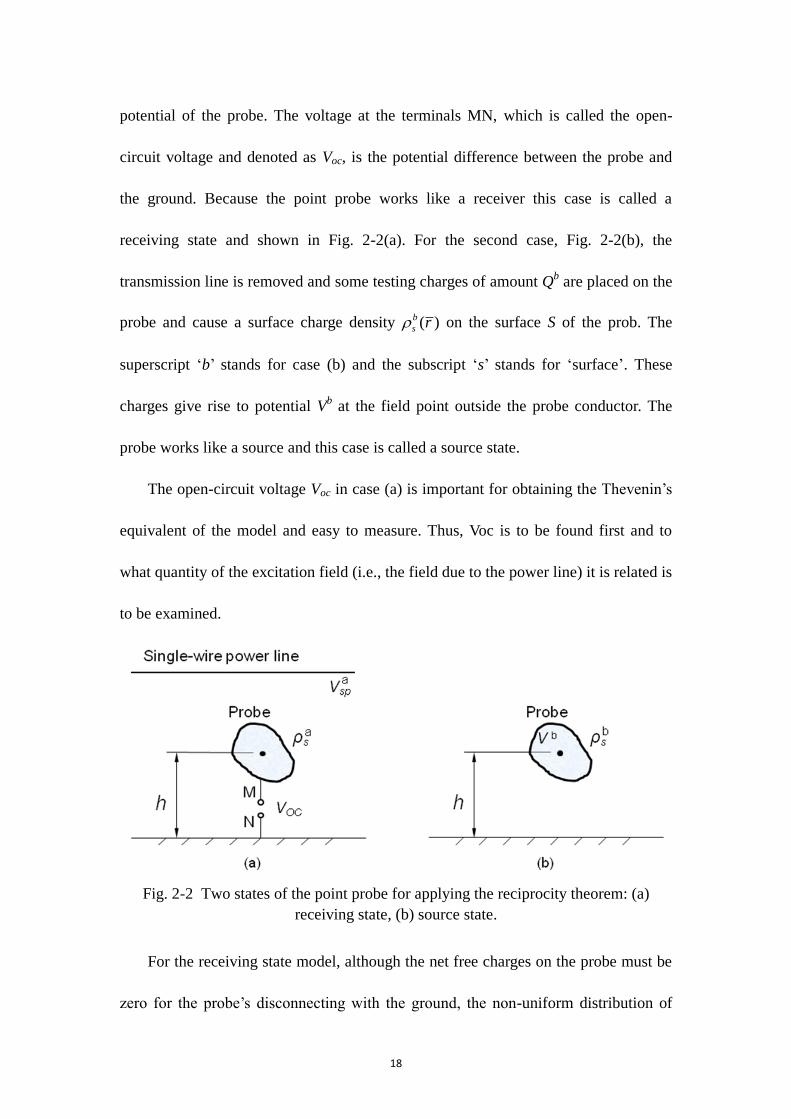
potential of the probe. The voltage at the terminals MN, which is called the open-

circuit voltage and denoted as Voc, is the potential difference between the probe and

the ground. Because the point probe works like a receiver this case is called a

receiving state and shown in Fig. 2-2(a). For the second case, Fig. 2-2(b), the

transmission line is removed and some testing charges of amount Qb are placed on the

probe and cause a surface charge density ( )b

s r on the surface S of the prob. The

superscript ‗b‘ stands for case (b) and the subscript ‗s‘ stands for ‗surface‘. These

charges give rise to potential Vb at the field point outside the probe conductor. The

probe works like a source and this case is called a source state.

The open-circuit voltage Voc in case (a) is important for obtaining the Thevenin‘s

equivalent of the model and easy to measure. Thus, Voc is to be found first and to

what quantity of the excitation field (i.e., the field due to the power line) it is related is

to be examined.

Fig. 2-2 Two states of the point probe for applying the reciprocity theorem: (a)

receiving state, (b) source state.

For the receiving state model, although the net free charges on the probe must be

zero for the probe‘s disconnecting with the ground, the non-uniform distribution of

19

the surface charge (with a density of ( )a

s r ) generates an electric field canceling the

excitation field due to the power line and keeping the total E field to be zero inside the

probe conductor. On the outside, the induced surface charge causes a potential of Va.

The space potential due to the power line in the absence of the probe is denoted as

a

SPV . It is clear that the total potential at each field point in the area is the superposition

of a

SPV and Va at that position. The open-circuit voltage Voc representing the total

potential on the probe surface can be written as

a a

SP ocV V V

Thus

(on )a a

SP ocV V V S (2.1)

Similarly, in Fig. 2-2(b), the potential is constant over S. Applying the reciprocity

theorem for electrostatics to this particular problem gives that [38]

( ) ( )b a a b

s s

S S

r V dS r V dS (2.2)

Inserting (2.1) into (2.2) yields

( ) 0b a b a

s oc SP s

S S

V V dS V dS (2.3)

Equation (2.3) can be equal to zero because the probe is ‗floating‘ in case (a) and the

net induced free charges on it are always zero. Then

b b a

s oc s SP

S S

V dS V dS

Because Voc is independent of the position variable, pulling it out of the integral on

the L.H.S. results

20

1 b a

oc s SPb

S

V V dSQ

(2.4)

From (2.4), the open-circuit voltage can be looked as the weighted average of the

unperturbed power line space potential over the surface of the point probe with the

weighting coefficient to be the charge on the probe surface. If the space potential and

the density of the testing charge are known on the probe surface, the open circuit

voltage Voc can be calculated.

Consider the case for which the probe conductor is small enough, such that the

space potential over S can be approximated as a constant and pulled out of the integral

in (2.4). Then the open circuit voltage can be rewritten as

a ab aSP SP

oc s b SP

b bS

V VV dS Q V

Q Q (2.5)

On the most right hand side of (2.5) is just the power line space potential a

SPV due

to the transmission line which equals to the open circuit voltage of the probe. Thus the

question asked at the beginning of section 2.2 has been answered by (2.5): placing an

point probe under a power line and measuring the open-circuit voltage of the point

probe results in the unperturbed space potential‘s being measured at the position of

the probe.

If the close the open terminals MN in Fig. 2-2(a) there will be an induced current

flowing through the grounding wire. This current can be easily measurable and can

also be calculated by finding the Thevenin‘s equivalent circuit for the probe model in

Fig. 2-2(a). Fig. 2-3(a) shows the Thevenin‘s equivalent circuit.

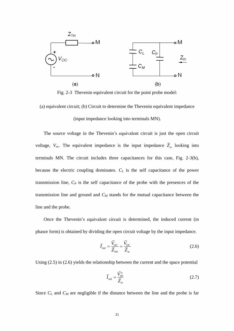
21

Fig. 2-3 Thevenin equivalent circuit for the point probe model:

(a) equivalent circuit; (b) Circuit to determine the Thevenin equivalent impedance

(input impedance looking into terminals MN).

The source voltage in the Thevenin‘s equivalent circuit is just the open circuit

voltage, Voc. The equivalent impedance is the input impedance inZ looking into

terminals MN. The circuit includes three capacitances for this case, Fig. 2-3(b),

because the electric coupling dominates. CL is the self capacitance of the power

transmission line, CP is the self capacitance of the probe with the presences of the

transmission line and ground and CM stands for the mutual capacitance between the

line and the probe.

Once the Thevenin‘s equivalent circuit is determined, the induced current (in

phasor form) is obtained by dividing the open circuit voltage by the input impedance.

OC OCind

TH in

V VI

Z Z (2.6)

Using (2.5) in (2.6) yields the relationship between the current and the space potential

a

SPind

in

VI

Z (2.7)

Since CL and CM are negligible if the distance between the line and the probe is far

22

enough (which is usually true for power transmission line and the point probe), the

input impedance of the probe is mainly determined by the capacitance of the probe,

CP. In addition, when the height of the probe h is large compared to its dimension (at

least 5 times of the largest dimension of the probe), the capacitance of the probe can

be approximated by its self-capacitance to free space [39], [40]. Finally a simple

expression of the induced current is obtained as

a

ind self SPI j C V (2.8)

where Cself is the self-capacitance of the point probe in free space without the

presences of the power line and the ground. For a spherical conductor with a radius of

a, its self-capacitance in free space is [40]

04selfC a (2.9)

where ε0 is the permittivity of free space. Usually, the self-capacitance of the point

probe is very small, which makes the coupling between the point probe and the power

lines is a high-impedance capacitive coupling. Therefore, the earth resistance of the

grounding system of the point probe can be neglected. According to (2.8), the induced

current is the product of the admittance of the probe‘s self-capacitance and the space

potential due to the power line. This provides us a means to find the space potential by

measuring the induced current of the point probe. In practice, by connecting an

ammeter between the probe and the ground, this induced current can be easily

measured. Using the measurement and (2.8) gives the space potential at the probe‘s

position.

All the analysis above is based on the model with a single-wire power

23

transmission line to be the excitation source. If the three-phase power transmission

line is the case, the analysis for each phase is similar to the previous one and the total

induced current of the probe should be obtained by the superposition of the results for

all the three phases. Then the total space potential is determined by (2.8).

2.3 Applications of point probe

2.3.1 Power line voltage monitoring

From the previous analysis, it is known that the point probe only picks up the electric

coupling from the power line and there is no magnetic coupling involved. As

discussed in Chapter 1, for the electromagnetic field produced by an energized power

transmission line the quasi-static approximation usually applies. The quasi-static

electric field is basically determined by the equivalent charges (i.e. the voltage) and

the configurations of the power line [17], [36]. This is also true for the space potential,

which is related to the electric field. Therefore, the most straightforward application

of the point probe is to monitor the voltage of the power line.

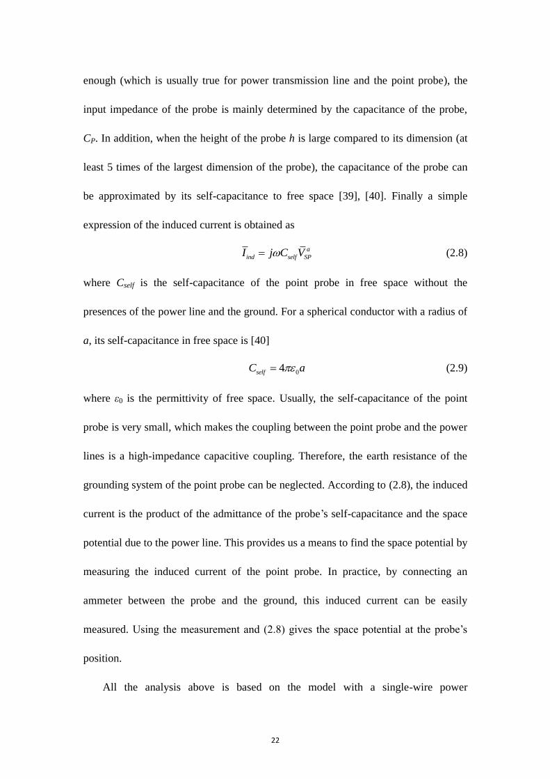
Fig. 2-4 depicts the configuration of a typical horizontal, 230kV, three-phase

power transmission line. Here, the ground is assumed to be perfect conductor and the

radius of the line conductor is 0.01m.

24

Fig. 2-4 Configuration of a 230kV, three phase, horizontal transmission line

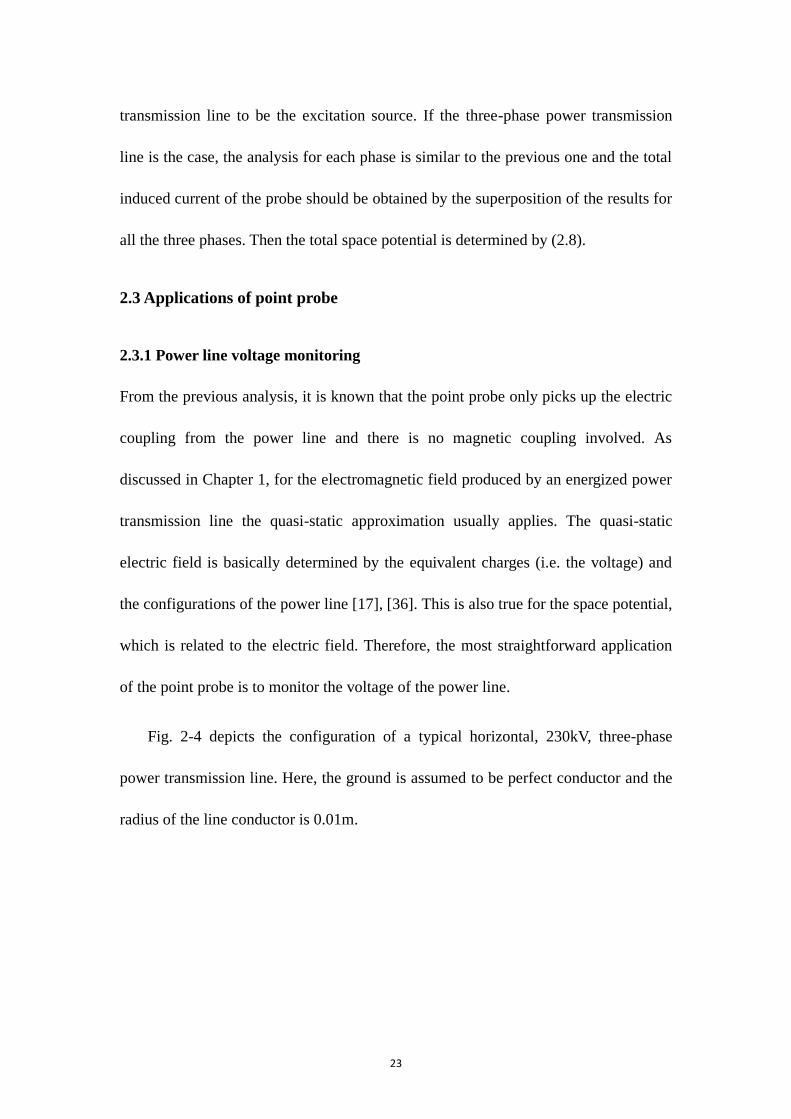
When a set of rating positive sequence voltages is applied on the line, the profiles

of space potential both in magnitude and phase are shown in Fig. 2-5. It is noticed that

the contours, both for magnitude and phase, have symmetries to the central vertical

axis.

(a) magnitude (kV) (b) phase angle (degree)

Fig. 2-5 Space potential profiles for positive sequence voltage

The total space potential at a field point is the superposition of the space

potentials caused by the three phase lines. And the space potential caused by each

25

phase is proportional to the voltage of that phase. So, the total space potential changes

linearly with the magnitude of the applied voltage on the power line.

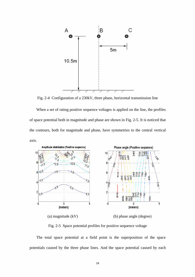
According to (2.8), if a grounded point probe is placed in the vicinity of the

power line, the space potential at the location of the probe can be determined by

measuring the induced current of the probe, illustrated in Fig. 2-6. The probe is placed

on the central axis of the cross section of the three-phase line. Consider (2.8) and the

analysis in last paragraph, the magnitude of the induced current changes linearly with

that of the applied voltage on the power line, too.

Fig. 2-6 Single probe placed under the three-phase power line

Fig. 2-7 shows the results of a simulation to find the relationship between the

power line voltage and the induced current in the point probe. The models of the

power line and the probe are the same as shown in Fig. 2-4 and Fig. 2-6, respectively.

The probe is a spherical conductor with radius of 7.6 cm (3 inch) and is 3 meters

above the ground. The applied voltage of the power line changes in between ±10% off

the rating voltage (230kV).

26

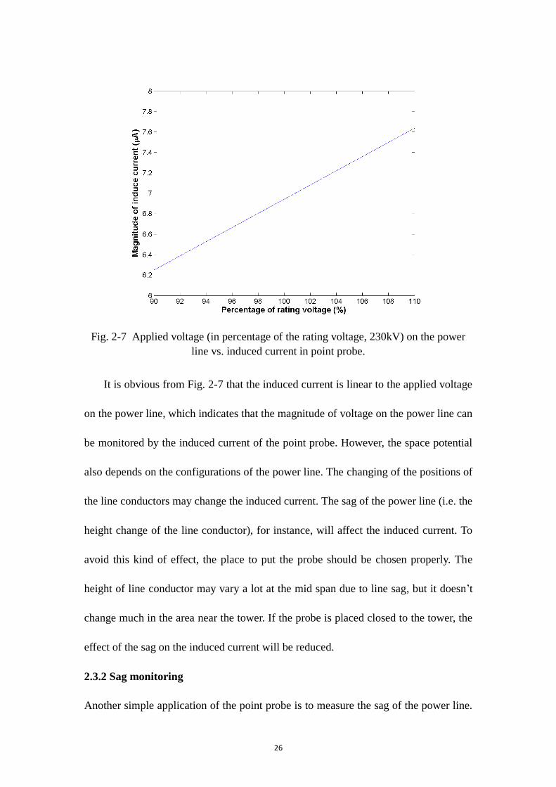
Fig. 2-7 Applied voltage (in percentage of the rating voltage, 230kV) on the power

line vs. induced current in point probe.

It is obvious from Fig. 2-7 that the induced current is linear to the applied voltage

on the power line, which indicates that the magnitude of voltage on the power line can

be monitored by the induced current of the point probe. However, the space potential

also depends on the configurations of the power line. The changing of the positions of

the line conductors may change the induced current. The sag of the power line (i.e. the

height change of the line conductor), for instance, will affect the induced current. To

avoid this kind of effect, the place to put the probe should be chosen properly. The

height of line conductor may vary a lot at the mid span due to line sag, but it doesn‘t

change much in the area near the tower. If the probe is placed closed to the tower, the

effect of the sag on the induced current will be reduced.

2.3.2 Sag monitoring

Another simple application of the point probe is to measure the sag of the power line.

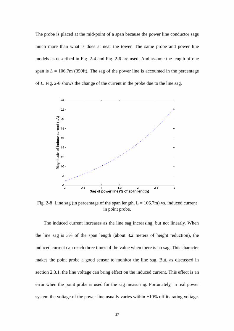
27

The probe is placed at the mid-point of a span because the power line conductor sags

much more than what is does at near the tower. The same probe and power line

models as described in Fig. 2-4 and Fig. 2-6 are used. And assume the length of one

span is L = 106.7m (350ft). The sag of the power line is accounted in the percentage

of L. Fig. 2-8 shows the change of the current in the probe due to the line sag.

Fig. 2-8 Line sag (in percentage of the span length, L = 106.7m) vs. induced current

in point probe.

The induced current increases as the line sag increasing, but not linearly. When

the line sag is 3% of the span length (about 3.2 meters of height reduction), the

induced current can reach three times of the value when there is no sag. This character

makes the point probe a good sensor to monitor the line sag. But, as discussed in

section 2.3.1, the line voltage can bring effect on the induced current. This effect is an

error when the point probe is used for the sag measuring. Fortunately, in real power

system the voltage of the power line usually varies within ±10% off its rating voltage.

28

On the other hand the sag of the line causes the height of the conductor to change in a

relatively large range at the mid-point of a span. The effect of the sag on the induced

current is much larger than that of the voltage. This is also proved by the level of the

magnitude change shown in Fig. 2-7 and Fig. 2-8.

2.3.3 Negative/Zero sequence voltage detection

The induced current and space potential in (2.8) are both phasors, which implies that

the information of both the magnitude and the phase of the space potential can be

obtained by the point probe if used in a proper way. Practically, the phase angle

information is hard to be picked up if only one probe is used. But if two or more

probes are applied the phase information can be utilized to accomplish more

complicated tasks than just measuring the magnitude of the space potential. A two-

probe system for the negative/zero sequence voltage detection is one example among

those applications.

Fig. 2-5 shows the positive space potential in both magnitude and phase angle. If

the negative sequence voltage is applied on the power line, the contours of the

magnitude and phase angle keep the same shapes, but the phase angle‘s distribution

changes, as shown in Fig. 2-9(b). Comparing Fig. 2-5 and Fig. 2-9, in most places in

the given cross sectional area the space potential phase changes under the different

sequence modes of power line voltage.

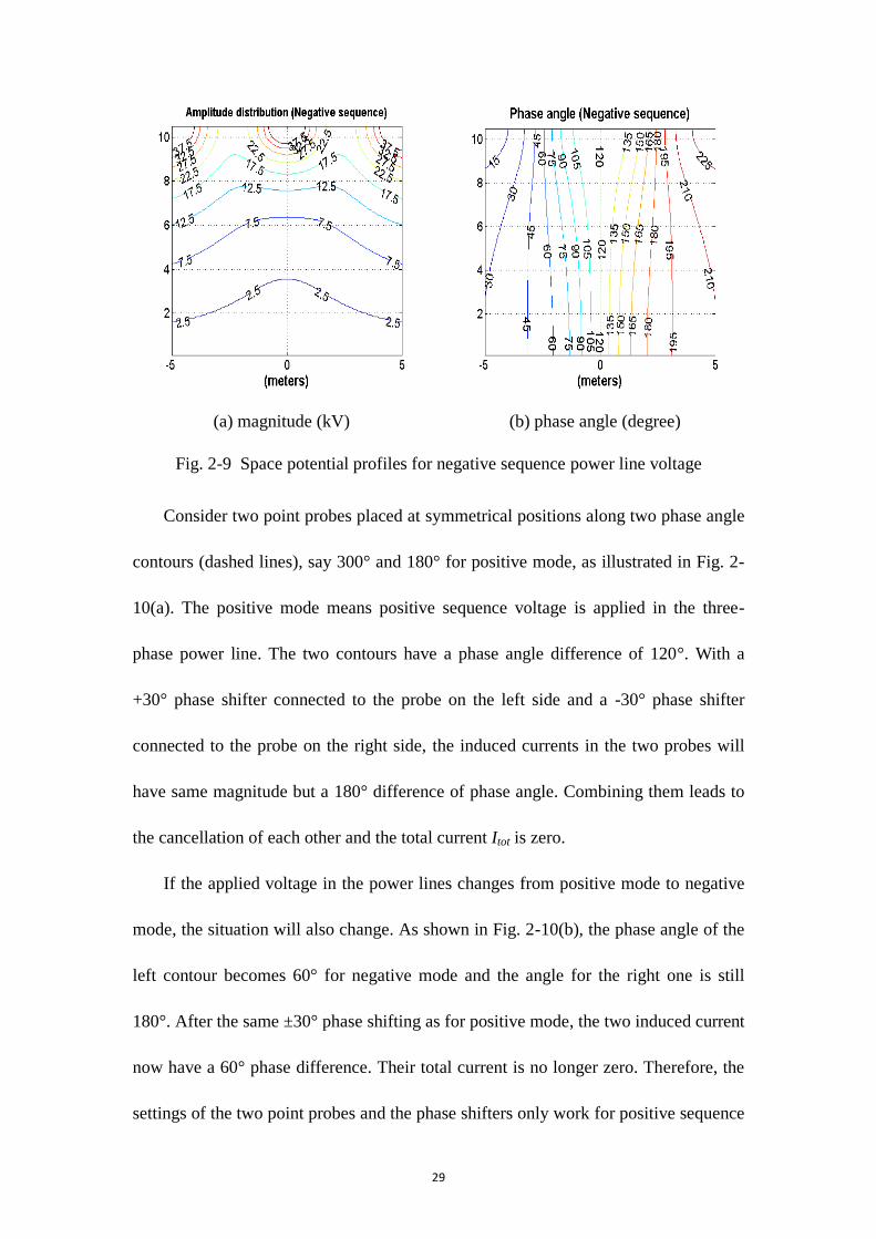
29

(a) magnitude (kV) (b) phase angle (degree)

Fig. 2-9 Space potential profiles for negative sequence power line voltage

Consider two point probes placed at symmetrical positions along two phase angle

contours (dashed lines), say 300° and 180° for positive mode, as illustrated in Fig. 2-

10(a). The positive mode means positive sequence voltage is applied in the three-

phase power line. The two contours have a phase angle difference of 120°. With a

+30° phase shifter connected to the probe on the left side and a -30° phase shifter

connected to the probe on the right side, the induced currents in the two probes will

have same magnitude but a 180° difference of phase angle. Combining them leads to

the cancellation of each other and the total current Itot is zero.

If the applied voltage in the power lines changes from positive mode to negative

mode, the situation will also change. As shown in Fig. 2-10(b), the phase angle of the

left contour becomes 60° for negative mode and the angle for the right one is still

180°. After the same ±30° phase shifting as for positive mode, the two induced current

now have a 60° phase difference. Their total current is no longer zero. Therefore, the

settings of the two point probes and the phase shifters only work for positive sequence

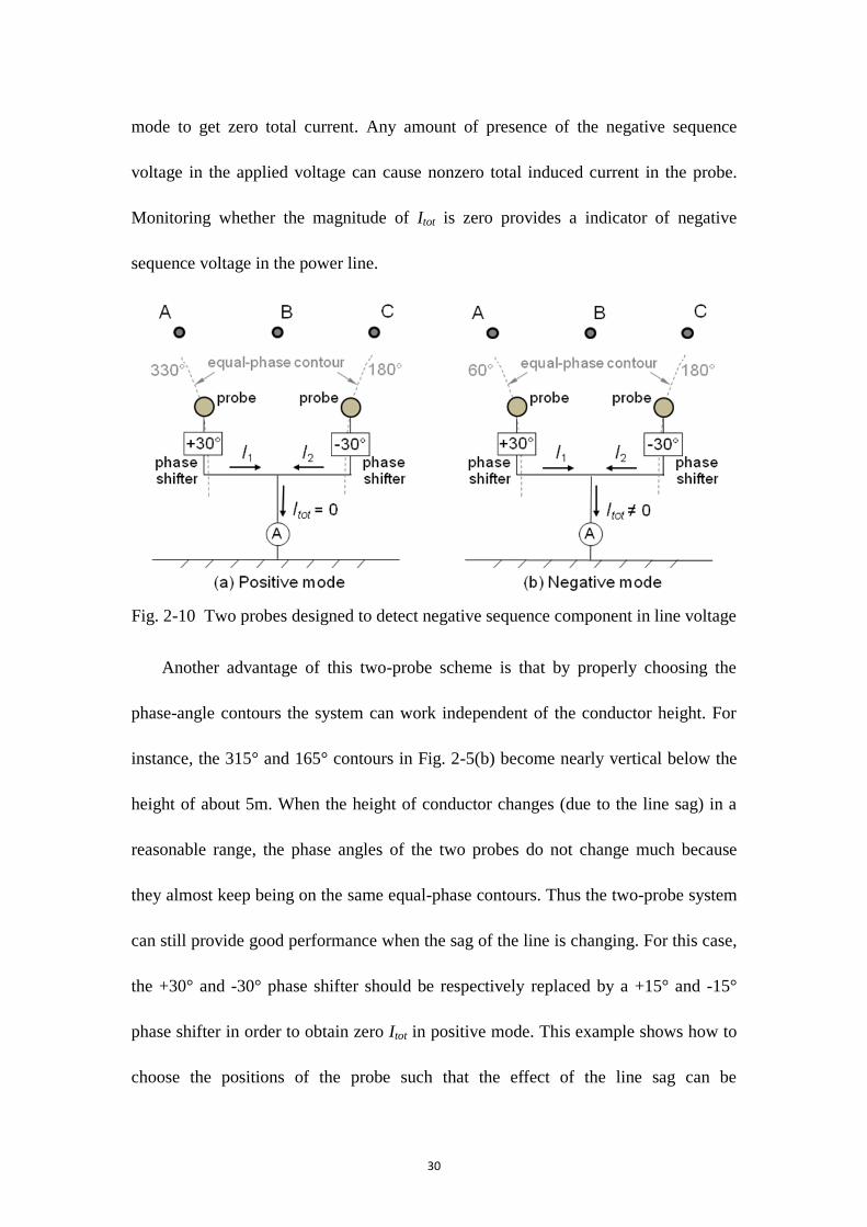
30

mode to get zero total current. Any amount of presence of the negative sequence

voltage in the applied voltage can cause nonzero total induced current in the probe.

Monitoring whether the magnitude of Itot is zero provides a indicator of negative

sequence voltage in the power line.

Fig. 2-10 Two probes designed to detect negative sequence component in line voltage

Another advantage of this two-probe scheme is that by properly choosing the

phase-angle contours the system can work independent of the conductor height. For

instance, the 315° and 165° contours in Fig. 2-5(b) become nearly vertical below the

height of about 5m. When the height of conductor changes (due to the line sag) in a

reasonable range, the phase angles of the two probes do not change much because

they almost keep being on the same equal-phase contours. Thus the two-probe system

can still provide good performance when the sag of the line is changing. For this case,

the +30° and -30° phase shifter should be respectively replaced by a +15° and -15°

phase shifter in order to obtain zero Itot in positive mode. This example shows how to

choose the positions of the probe such that the effect of the line sag can be

31

significantly mitigated. However, sometimes it is an advantage to use the dependence

of phase angle on the line sag (i.e., conductor height). Then the point probe must be

placed in the areas in which the equal-phase contours have slow slope. Because in

these areas the phase angle of space potential is sensitive to the conductor height. The

induced current is consequently sensitive to the change of conductor height.

Once the mechanism of two-probe system is well understood, it‘s not difficult to

update the system with the three-probe model. Using three probes allow us to built a

device to indicate the four operating modes in the power transmission line: positive

mode, negative mode, zero mode (zero sequence voltage is applied) and unenergized

mode (the power line is unenergized). One example for the three-probe approach is

illustrated in Fig. 2-11. Three identical probes are located on one equal-magnitude

contour (dotted line). The middle probe is on the central axis and the other two are put

on two symmetrical phase-angle contours (dashed lines). As shown in Fig. 2-11(a),

the phase-angle contours of 270° and 210° (for positive sequence) are chosen to place

the probes on. The central phase-angle contour has the angle value of 240°. The angle

shifting is -90° for the left phase shifter and +90° for the right one.

32

Fig. 2-11 Design of a three-probe device used as a four-mode indicator

The two ammeters A0 and A

- are the indicators for zero mode and negative mode,

respectively. The reading on A0 is zero when the applied voltage on the power line is

in zero mode and reading on A- is zero when negative mode is on. If both of the two

meters show nonzero readings there is only positive-sequence voltage operating.

When the transmission line is not energized, there will be no induced current in any of

the three probes. Hence, by inspecting the current in one single probe, the out-of-

service mode of the line can also be indicated by this device. Table 2-1 shows the

corresponding current statuses for each of the four modes.

Table 2-1 Four sequence modes and their corresponding current statuses

Mode 1,2 3orI

0I I

Positive ≠ 0 ≠ 0 ≠ 0

Negative ≠ 0 ≠ 0 0

Zero ≠ 0 0 ≠ 0

Out-of-service 0 0 0

It is not often true in the real power system that only one sequence of voltage

operates in the power line. The unbalanced operations or faults can cause the

33

presences of the negative and zero sequence components in line voltage. Consider the

case that both positive sequence and negative sequence components are present at the

same time. It is good for protection relay engineer to know the magnitude ratio of the

negative sequence to the positive sequence voltage. Since the phase of the space

potential depends on the sequence of the line voltage, one may be inspired that the

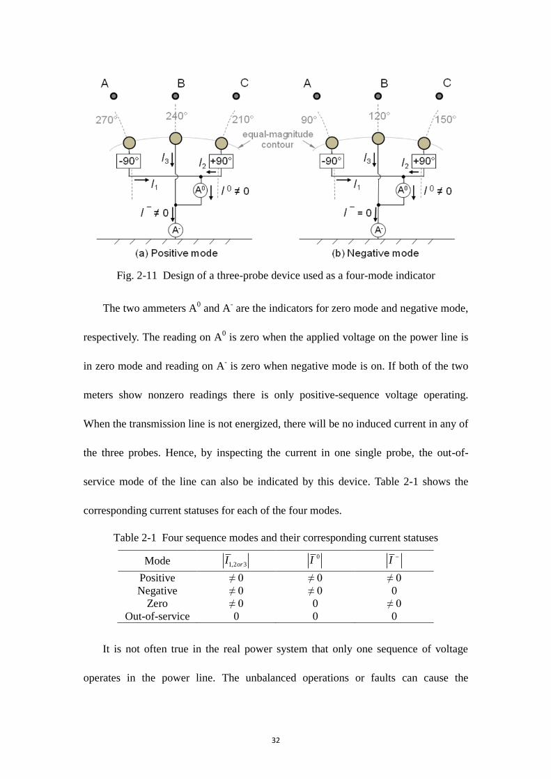
point probe can be used for accomplishing this task. Here is a design, Fig. 2-12, of a

three-probe device by which the ratio of the negative to positive sequence line voltage

can be found.

Fig. 2-12 Design of a negative-to-positive ratio measurement device

Similar analysis applies as before. If the contours of 255° and 225° (for positive

mode) are chosen, in the negative mode they have angles of 105° and 135°,

respectively. The angle shiftings are chosen to be ±105°. The two ammeters Ap and An

are set to respectively measure the magnitude of the induced current for positive and

negative modes. This is valid because for the settings shown in Fig. 2-12 it is always

true that

34

0nI and 240pI I

where I+ is the magnitude of positive sequence current in the probes and the

superscript ‗+‘ stands for quantities in positive mode. The positive currents from the

two side probes always cancel each other because they have 180° angle difference

after phase shifting. Thus, in the reading of ammeter An positive sequence current is

always zero. The ammeter An will only measure the magnitude of negative sequence

current. Similarly

300nI I and 0pI

where I- is the magnitude of negative sequence current in the probes the superscript ‗-‘

stands for quantities in negative mode and. Combining the currents for the two

sequence modes shows that the reading on Ap is only the magnitude of positive

sequence current p p p pI I I I and the reading on An is only the magnitude of

negative sequence current n n n nI I I I . Thus

300

240

n

p

II I

II I

(2.10)

From the analysis in section 2.2, the induced current is proportional to the line voltage

in magnitude, which results in that

line n

pline

V I I

IIV

(2.11)

The theory introduced in this example is verified by computer simulation. In the

simulation, the positions to locate the three probes have the coordinates (in meters) as

(-0.414, 2.98), (0, 3.08), and (0.414, 2.98). Apply a series of three-phase line voltage

which contain different percentages of negative sequence. Calculate the current ratio

35

by (2.10). Table 2-2 lists the results. The error is due to the position of the probes.

Table 2-2 Results for computer simulation

line

line

V

V

5.0% 10.0% 15.0% 20.0% 25.0% 30.0% 35.0% 40.0%

n

p

I

I 4.9% 9.8% 14.7% 19.6% 24.5% 29.5% 34.4% 39.3%

2.4 Lab tests and field experiments of point probe

Some lab tests and field experiments have been conducted to validate the theories of

the point probe.

2.4.1 Single-phase, single-probe lab test

This test is to check whether the modeling of space potential probe works as presented

in (2.8). Voltage is applied on one bus bar to simulate a single-phase power

transmission line. A spherical conducting probe supported by a PVC pipe locates right

below the bar, as illustrated in Fig. 2-13. The probe is grounded by one coaxial cable.

The induced current is measured by a ―FLUKE 189‖ ammeter. By using (2.2) the

space potential is obtained from the induced current. To verify the result, the space

potential at where the probe is placed is also directly measured by a space potential

meter (see Fig. 2-14). The two potential values, one computed from the current and

one measured directly, are compared in Table 2-3.

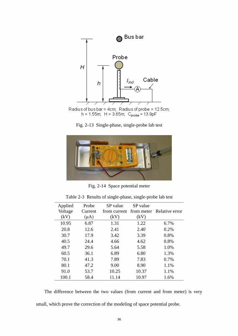
36

Fig. 2-13 Single-phase, single-probe lab test

Fig. 2-14 Space potential meter

Table 2-3 Results of single-phase, single-probe lab test

Applied

Voltage

(kV)

Probe

Current

(μA)

SP value

from current

(kV)

SP value

from meter

(kV)

Relative error

10.95 6.87 1.31 1.22 6.7%

20.8 12.6 2.41 2.40 0.2%

30.7 17.9 3.42 3.39 0.8%

40.5 24.4 4.66 4.62 0.8%

49.7 29.6 5.64 5.58 1.0%

60.5 36.1 6.89 6.80 1.3%

70.1 41.3 7.89 7.83 0.7%

80.1 47.2 9.00 8.90 1.1%

91.0 53.7 10.25 10.37 1.1%

100.1 58.4 11.14 10.97 1.6%

The difference between the two values (from current and from meter) is very

small, which prove the correction of the modeling of space potential probe.

37

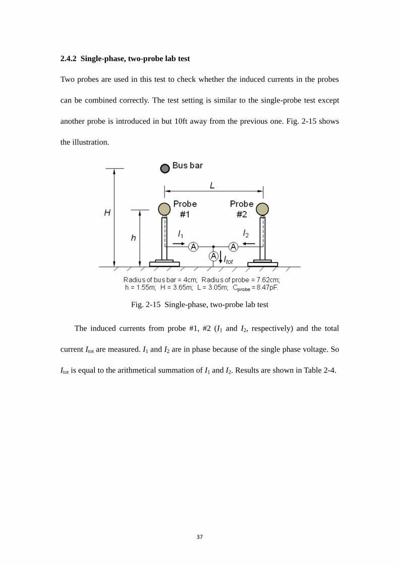
2.4.2 Single-phase, two-probe lab test

Two probes are used in this test to check whether the induced currents in the probes

can be combined correctly. The test setting is similar to the single-probe test except

another probe is introduced in but 10ft away from the previous one. Fig. 2-15 shows

the illustration.

Fig. 2-15 Single-phase, two-probe lab test

The induced currents from probe #1, #2 (I1 and I2, respectively) and the total

current Itot are measured. I1 and I2 are in phase because of the single phase voltage. So

Itot is equal to the arithmetical summation of I1 and I2. Results are shown in Table 2-4.

38

Table 2-4 Results of single-phase, two-probe test

Applied

Voltage (kV)

Current of

Probe #1, I1

(μA)

Current of

Probe #2, I2

(μA)

Total Probe

Current, Itot

(μA)

I1+I2

(μA)

15.4 9.79 3.43 12.82 13.22

21.1 10.67 3.94 14.23 14.61

31.5 14.37 5.73 19.49 20.10

40.8 17.21 7.08 23.58 24.29

51.0 21.03 8.43 28.82 29.46

61.5 22.34 8.75 30.46 31.09

69.6 24.76 9.85 34.34 34.61

81.1 28.51 11.24 39.42 39.75

91.6 32.26 12.82 44.86 45.08

102.8 36.06 14.28 50.05 50.34

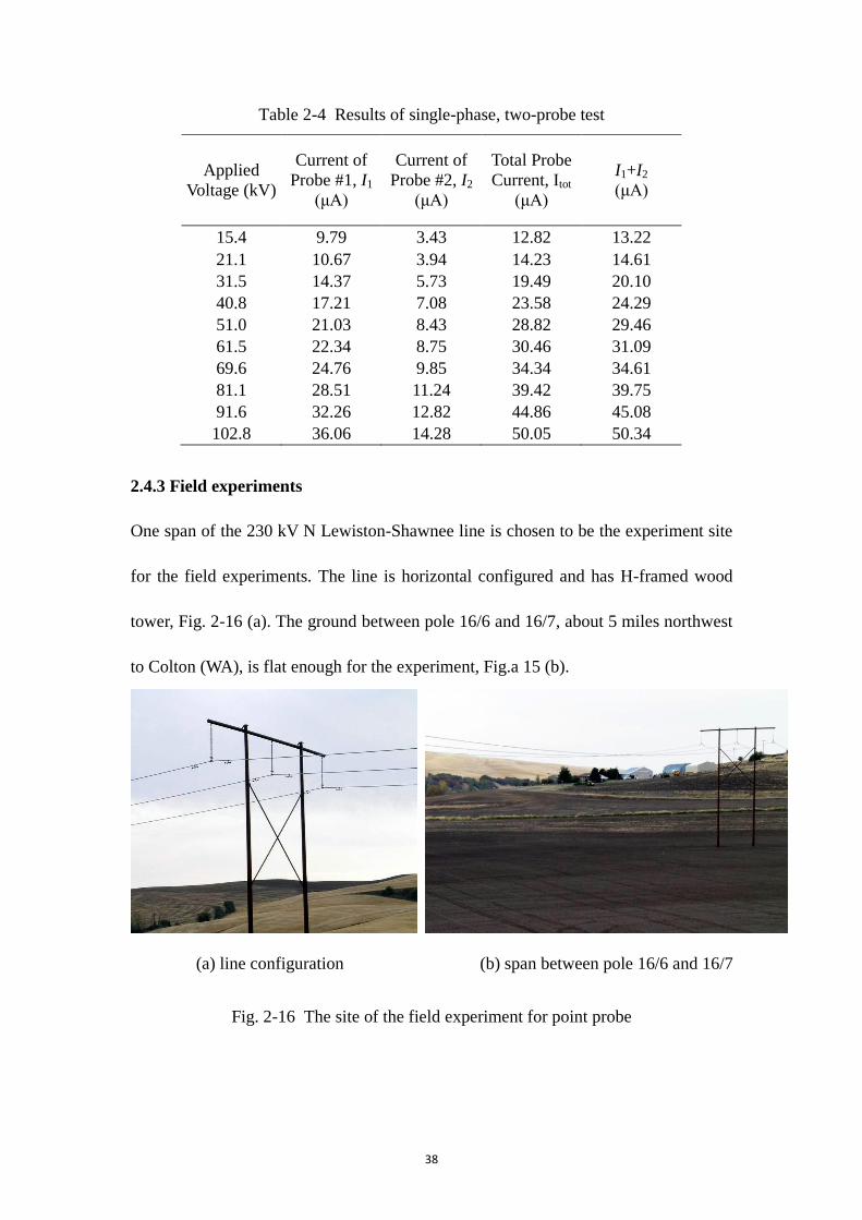
2.4.3 Field experiments

One span of the 230 kV N Lewiston-Shawnee line is chosen to be the experiment site

for the field experiments. The line is horizontal configured and has H-framed wood

tower, Fig. 2-16 (a). The ground between pole 16/6 and 16/7, about 5 miles northwest

to Colton (WA), is flat enough for the experiment, Fig.a 15 (b).

(a) line configuration (b) span between pole 16/6 and 16/7

Fig. 2-16 The site of the field experiment for point probe

39

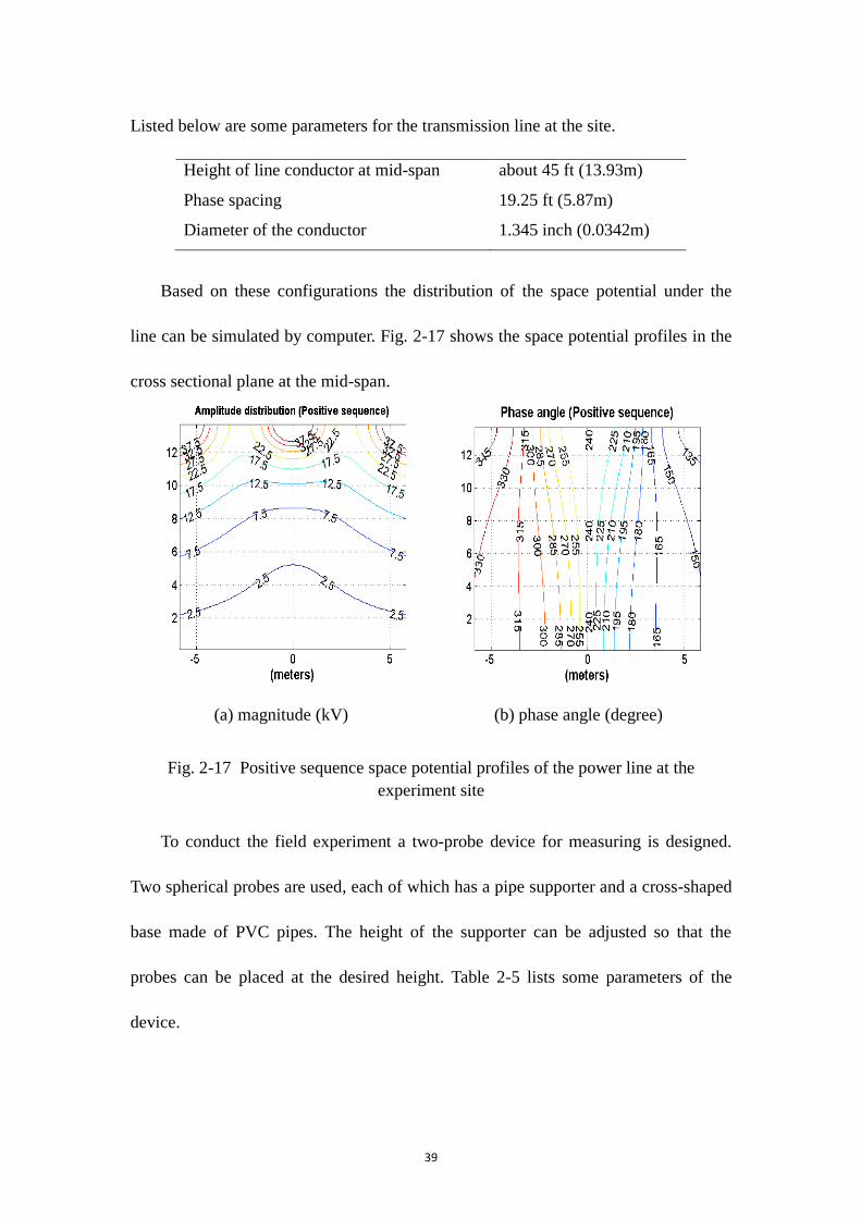
Listed below are some parameters for the transmission line at the site.

Height of line conductor at mid-span about 45 ft (13.93m)

Phase spacing 19.25 ft (5.87m)

Diameter of the conductor 1.345 inch (0.0342m)

Based on these configurations the distribution of the space potential under the

line can be simulated by computer. Fig. 2-17 shows the space potential profiles in the

cross sectional plane at the mid-span.

(a) magnitude (kV) (b) phase angle (degree)

Fig. 2-17 Positive sequence space potential profiles of the power line at the

experiment site

To conduct the field experiment a two-probe device for measuring is designed.

Two spherical probes are used, each of which has a pipe supporter and a cross-shaped

base made of PVC pipes. The height of the supporter can be adjusted so that the

probes can be placed at the desired height. Table 2-5 lists some parameters of the

device.

40

Table 2-5 Parameters of the two-probe device

Radius of probe 3 in (0.0762m)

Height range of supporter 6~10.5ft, adjustable

Dimension of base 8×8ft, diagonal

Minimum current recognized 0.01μA

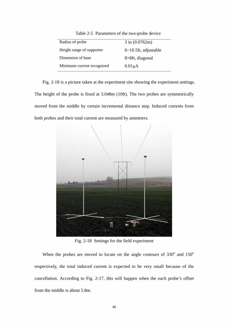
Fig. 2-18 is a picture taken at the experiment site showing the experiment settings.

The height of the probe is fixed at 3.048m (10ft). The two probes are symmetrically

moved from the middle by certain incremental distance step. Induced currents from

both probes and their total current are measured by ammeters.

Fig. 2-18 Settings for the field experiment

When the probes are moved to locate on the angle contours of 330o and 150

o

respectively, the total induced current is expected to be very small because of the

cancellation. According to Fig. 2-17, this will happen when the each probe‘s offset

from the middle is about 5.8m.

41

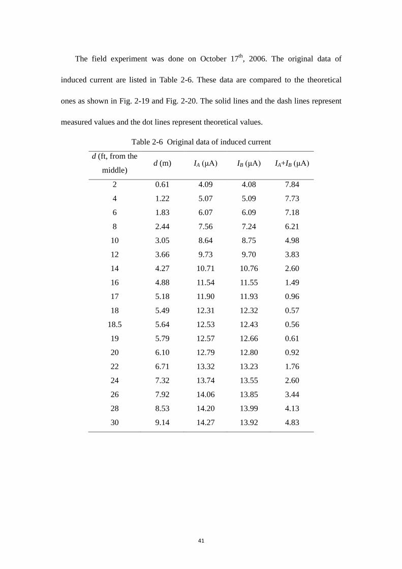
The field experiment was done on October 17th

, 2006. The original data of

induced current are listed in Table 2-6. These data are compared to the theoretical

ones as shown in Fig. 2-19 and Fig. 2-20. The solid lines and the dash lines represent

measured values and the dot lines represent theoretical values.

Table 2-6 Original data of induced current

d (ft, from the

middle) d (m) IA (μA) IB (μA) IA+IB (μA)

2 0.61 4.09 4.08 7.84

4 1.22 5.07 5.09 7.73

6 1.83 6.07 6.09 7.18

8 2.44 7.56 7.24 6.21

10 3.05 8.64 8.75 4.98

12 3.66 9.73 9.70 3.83

14 4.27 10.71 10.76 2.60

16 4.88 11.54 11.55 1.49

17 5.18 11.90 11.93 0.96

18 5.49 12.31 12.32 0.57

18.5 5.64 12.53 12.43 0.56

19 5.79 12.57 12.66 0.61

20 6.10 12.79 12.80 0.92

22 6.71 13.32 13.23 1.76

24 7.32 13.74 13.55 2.60

26 7.92 14.06 13.85 3.44

28 8.53 14.20 13.99 4.13

30 9.14 14.27 13.92 4.83

42

Fig. 2-19 Probe currents of the field experiments

Fig. 2-20 Total current of the field experiments

43

This experiment is a simplified implementation of the two-probe approach. The

positive sequence voltage is assumed to be applied in the power line and no phase

shifters are used. The results validate the theory that the current cancels at certain

positions of the probes. The zero total current occurs when the probes are placed at

the same positions as predicted. Therefore, this experiment proves that the phase

angle information can be picked up and utilized by using the point probe and it also

indirectly proves the theories for the negative/zero sequence voltage detection

discussed in section 2.3.3.

44

CHAPTER 3

GENERAL THEORY OF LINEAR SENSORS

The linear sensor is the type of electromagnetic (EM) sensor to be studied in Chapter

3 to 5 of this dissertation. It has a wire-like shape, which differs from the point probe

in Chapter 2. Since the analysis for the linear sensor is based on the reciprocity

theorem, which places no special requirements on the sensor shape, there are not

many shape constraints made on the model of the linear sensor. For example, it sensor

is not necessary that the sensor be straight or be uniform in diameter. The wire-like

EM sensor has many practical applications in high frequency areas, but its application

in low frequency system such as electric power system at 60Hz is seldom seen in the

literature. Important objectives of this dissertation are to derive a theory and to

propose potential applications for using the linear sensor in EM measurement of

power transmission line status.

In this chapter the theory behind the linear sensor will be explored. An approach

based on the reciprocity theorem for general electromagnetic case is introduced in 3.1.

A solution to the induced current in a linear sensor excited by the incident

electromagnetic field is then provided. Following this, an approach using the model of

per-unit-length induced voltage and current sources is introduced in 3.2. Finally, the

relationship between the two approaches is discussed in 3.3.

3.1 Approach by reciprocity theorem

A general model of the linear sensor to be used in the following sections is depicted in

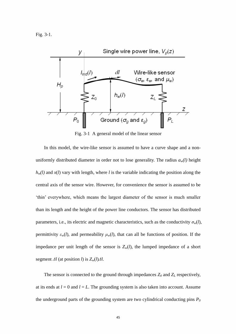
45

Fig. 3-1.

Fig. 3-1 A general model of the linear sensor

In this model, the wire-like sensor is assumed to have a curve shape and a non-

uniformly distributed diameter in order not to lose generality. The radius aw(l) height

hw(l) and x(l) vary with length, where l is the variable indicating the position along the

central axis of the sensor wire. However, for convenience the sensor is assumed to be

‗thin‘ everywhere, which means the largest diameter of the sensor is much smaller

than its length and the height of the power line conductors. The sensor has distributed

parameters, i.e., its electric and magnetic characteristics, such as the conductivity ζw(l),

permittivity εw(l), and permeability μw(l), that can all be functions of position. If the

impedance per unit length of the sensor is Zw(l), the lumped impedance of a short

segment Δl (at position l) is Zw(l)Δl.

The sensor is connected to the ground through impedances Z0 and ZL respectively,

at its ends at l = 0 and l = L. The grounding system is also taken into account. Assume

the underground parts of the grounding system are two cylindrical conducting pins P0

46

and PL, which vertically penetrate into the lossy earth with dielectric constant of εg

and conductivity of ζg. The grounding impedances of the two pins are Zp0 and ZpL,

respectively. The sensor itself along with impedances Z0 and ZL, grounding

impedances Zp0 and ZpL, and the earth return form a sensor system, which is placed

under a power transmission line.

The power line, with an applied voltage of Vp(z) on it, is a single, horizontal and

infinitely extending wire in ‗z‘ direction. The power line conductor has a radius of a

(meters) and is H (meters) above the ground. The applied voltage Vp(z) is a 60Hz

sinusoid, for which the free space wavelength λ0 is 5000km. Thus the sensor is

electrically short (i.e., length of the sensor << λ0) for most cases. But in some special

cases, high speed transient processes for instance, the sensor may not be electrically

short. The manner in which the sensor is placed is not specified in this model. It could

be placed parallel, oblique, or perpendicular to the power line‘s axial direction, i.e., z

direction. Models with the sensor placed perpendicular and parallel to the power line

are to be studied in Chapter 4 and Chapter 5, respectively.

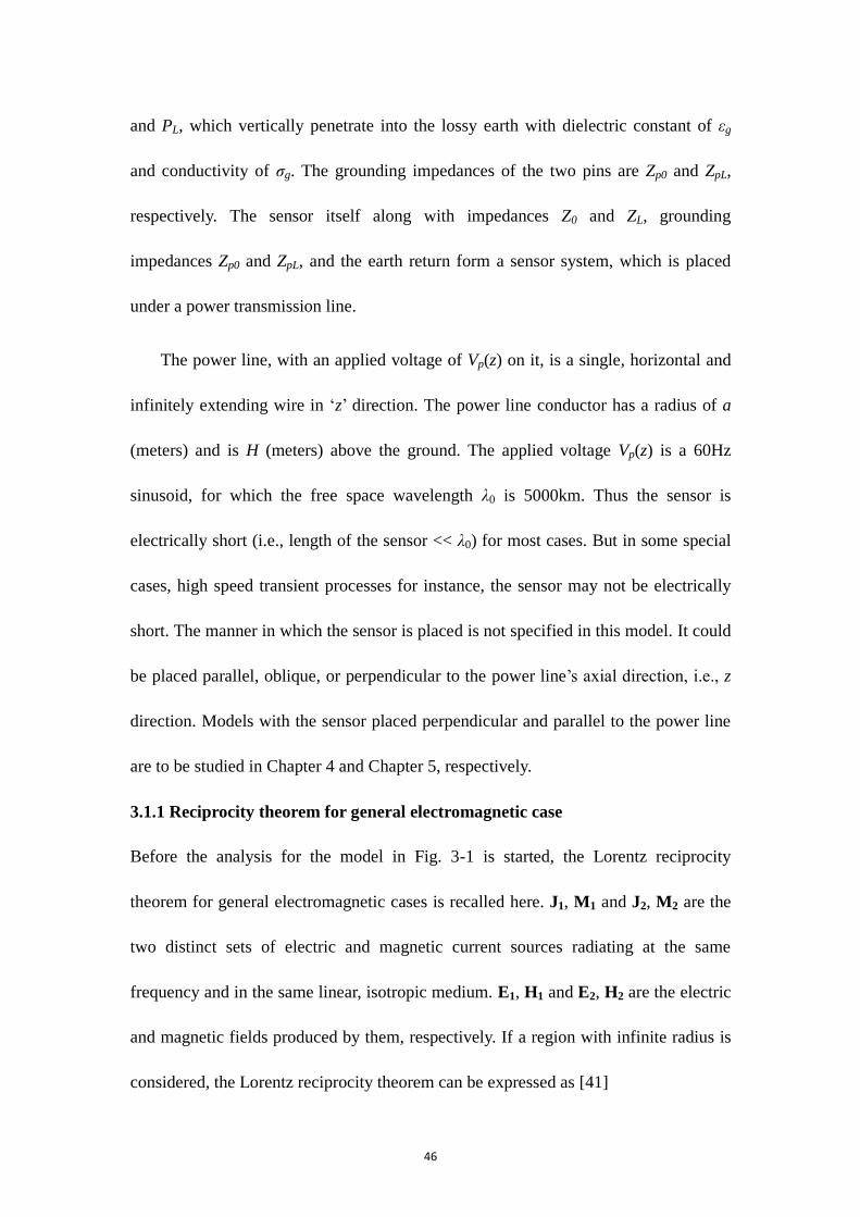
3.1.1 Reciprocity theorem for general electromagnetic case

Before the analysis for the model in Fig. 3-1 is started, the Lorentz reciprocity

theorem for general electromagnetic cases is recalled here. J1, M1 and J2, M2 are the

two distinct sets of electric and magnetic current sources radiating at the same

frequency and in the same linear, isotropic medium. E1, H1 and E2, H2 are the electric

and magnetic fields produced by them, respectively. If a region with infinite radius is

considered, the Lorentz reciprocity theorem can be expressed as [41]

47

1 2 1 2 1V V

dv dv 1 2 2E J H M E J H M (3.1)

For the case without magnetic current sources (M1 = M2 = 0), (3.1) reduces to

2 1V V

dv dv 1 2E J E J (3.2)

Particularly, consider the case that the source J1 and J2 are the currents on two wires

(i.e. two line currents), w1 and w2, respectively, as illustrated in Fig. 3-2.

Fig. 3-2 Special case for reciprocity theorem: sources reduces to line currents (J1 and

J2)

The volume integral in (3.2) reduces to line integral. Thus, the reciprocity theorem for

this special case can be presented as

2 12 1

w wdl dl 1 2E J E J (3.3)

Equation (3.3) is very important and it will be used to derive the basic theory for the

linear sensor in the following sections.

3.1.2 Two situations for implementing reciprocity theorem

Equation (3.3) will now be used to study the linear sensor model shown in Fig. 3-1.

Basically, the sensor is a receiving antenna. In the antenna theory, one important

problem is to determine the current distribution on the antenna [18]. Thus, the goal

here is to find the induced current and voltage everywhere on the sensor when it is

excited by the electromagnetic field produced by the power line. The approach is to

determine the Thevenin equivalent circuit of the sensor at an arbitrary position along

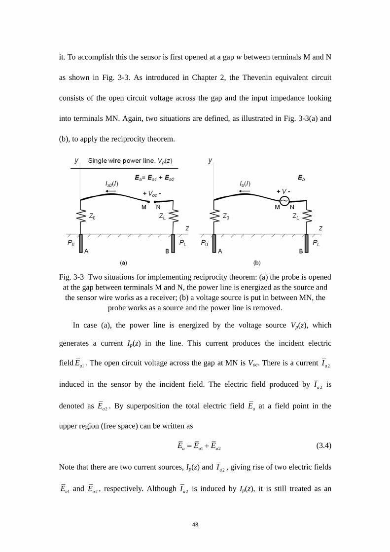
48

it. To accomplish this the sensor is first opened at a gap w between terminals M and N

as shown in Fig. 3-3. As introduced in Chapter 2, the Thevenin equivalent circuit

consists of the open circuit voltage across the gap and the input impedance looking

into terminals MN. Again, two situations are defined, as illustrated in Fig. 3-3(a) and

(b), to apply the reciprocity theorem.

Fig. 3-3 Two situations for implementing reciprocity theorem: (a) the probe is opened

at the gap between terminals M and N, the power line is energized as the source and

the sensor wire works as a receiver; (b) a voltage source is put in between MN, the

probe works as a source and the power line is removed.

In case (a), the power line is energized by the voltage source Vp(z), which

generates a current Ip(z) in the line. This current produces the incident electric

field 1aE . The open circuit voltage across the gap at MN is Voc. There is a current 2aI

induced in the sensor by the incident field. The electric field produced by 2aI is

denoted as 2aE . By superposition the total electric field aE at a field point in the

upper region (free space) can be written as

1 2a a aE E E (3.4)

Note that there are two current sources, Ip(z) and 2aI , giving rise of two electric fields

1aE and 2aE , respectively. Although 2aI is induced by Ip(z), it is still treated as an

49

independent source. 2aI and

2aE form one source-field pair in the following analysis

for applying the reciprocity theorem.

In case (b), the power line and the voltage source Vp(z) are removed. Instead, a

voltage source with amplitude of V is connected to the terminals M and N. The probe

is acting as a source now. Assume the current produced by V on the probe is bI and

the electric field at the field point due to this current is bE . bI and bE make another

source-field pair for using the reciprocity theorem.

3.1.3 Implementing reciprocity theorem

The induced current 2aI in case (a) produces electric field 2aE and the source current

bI in case (b) produces electric field bE . Thus, bI and 2aI are the two sources and bE

and 2aE are the fields respectively excited by them. Replacing the current sources and

the electric fields in (3.3) by the following relationships

2 2

( ) , ( ) ,

( ) , ( ) ,

b b

a a

I l E l

I l E l

1 1

2 2

J E

J E

(3.3) can be rewritten as

2 2( ) ( ) ( ) ( )AB AB

b a a bC C

E l I l dl E l I l dl (3.5)

where CAB is the contour that covered by the whole sensor system, from the lower

ends of the grounding pin P0 to that for PL, i.e., from A Z0 M N ZL B. It

includes, from left to right hand side, P0, Z0, the sensor, the gap w, ZL and PL. In fact,

the whole loop of the circuit includes an earth return, too. There should be a current

flowing in the earth if it is not perfect conductor. In (3.5), however, the integral term

associated with this earth return current hasn‘t been explicitly expressed because the

50

effect of the earth return current can be fully accounted in the expression of the

incident field 1aE . If the earth is perfect conductor, this return current effect on the

incident field can be replaced by an image current. If the earth is lossy, its effect can

be represented by a Carson‘s term in the incident field formulation [26]. The details

about this issue will be discussed in later section.

The currents and the electric fields are all vectors and functions of position.

Actually, the spatial vector of current can be presented as

2 2ˆ ˆ( ) ( ) and ( ) ( )a l a b l bI l a I l I l a I l

where ˆla is the unit spatial vector pointing in the same direction as the sensor‘s

central axis, and 2 ( )aI l , ( )bI l are the magnitudes of the corresponding currents. For

the position vector on the sensor

ˆldl a dl

With these relations (3.5) is equivalent to

2 2( ) ( ) ( ) ( )AB AB

a b b aC C

I l E l dl I l E l dl (3.6)

Because the induced current 2aI in the gap is zero, the left-hand side of (3.6) can be

rewritten as

2L.H.S. ( ) ( )AM NB

a bC C

I l E l dl

(3.7)

Equation (3.7) is valid because there is no current flowing through the gap if the

sensor wire is open. Thus Ia2(gap) = 0, which causes the integral term

2 ( ) ( )a bgap

I l E l dl to be zero.

On the right-hand side, if the gap is small enough, the current through the gap

( )bI gap can be approximated as a constant. Additionally, replacing 2aE by (3.4)

51

1R.H.S. ( ) ( ) ( ) ( )AB AB

b a b aC C

I l E l dl I l E l dl

Separating the integral over the gap from the first term and simplifying it, the R.H.S.

becomes

1R.H.S. ( ) ( ) ( ) ( ) ( )AM NB AB

b a b oc b aC C C

I l E l dl I gap V I l E l dl

(3.8)

where Ib(gap) is the current Ib at the position of the gap, Voc is the open circuit voltage

across MN, and ( )oc agap

V E l dl .

The dot product of the electric field with the position vector at the field point is

the tangential field component multiplied by the incremental length, i.e., the voltage

across the incremental sensor segment. Thus

2a a w

b b w

E dl dV I Z dl

E dl dV I Z dl

(3.9)

where Zw is the per unit length surface impedance (Ω/m) of the sensor [42]. Inherently,

that (3.9) is valid is based on the thin wire assumption of the sensor wire. The sensor

wire is assumed to be thin wire so that the tangential electric field on the surface of

the wire is equal to the product of the surface impedance of the wire conduct and the

current [42]. In addition, for the lumped impedance Z0 and ZL, it is true that

0 2 0 2

0 0

;

;

a a

a L a L

b b

b L b L

V I Z V I Z

V I Z V I Z

(3.10)

where 0

aV is the voltage on Z0 due to Ia2, a

LV is the voltage on ZL due to Ia2, 0

bV is the

voltage on Z0 due to Ib and b

LV is the voltage on ZL due to Ib. Inserting (3.9) and (3.10)

into (3.7) and (3.8),

2 0 2 2

2 1 0

( ) ( )

( ) ( ) ( ) ( )

AM NB

AM NB AB

b b

a b S a L aC C

a a

b a S b oc b a b L bC C C

I l I l Z dl V I V I

I l I Z dl I w V I l E l dl V I V I

52

According to the reciprocity theorem for lumped elements, it holds that

0 2 0

2

b a

a b

b a

L a L b

V I V I

V I V I

Thus, the four terms relative to the lumped impedance in the previous equation can be

cancelled. Finally, the relationship between the open-circuit voltage and the incident

electric field due to the power line is found as

1( ) ( ) ( )AB

b oc b aC

I gap V I l E l dl

and can be written as

1

1( ) ( )

( ) ABoc b a

Cb

V I l E l dlI gap

(3.11)

Equation (3.11) is the expression of ‗hybrid reciprocity theorem‘ [43] – [46]. Mapping

this theorem to our linear sensor problem it is known that the open circuit voltage at

the terminals MN can be calculated if the incident electric field 1( )aE l due to the

power line and the distribution of the current ( )bI l when the probe is driven by a

voltage source V are known. In (3.11), 1aE is nothing but the electric field generated

by an infinite long horizontal conductor wire above earth without the presence of the

sensor. Fortunately, the electromagnetic field exited by an infinite long wire above

earth is a canonical problem and has been studied since the 1920‘s [26]. So electric

field in (3.11) is not difficult to obtain. The current distribution ( )bI l may be difficult

to be determined for the general case, but if the linear sensor is a straight horizontal

wire, the current due to a voltage source V can be calculated by the classical

transmission theory.

Finding the open circuit voltage is only half of the problem of determining the

Thevenin‘s equivalent circuit. The other half is to calculate the Thevenin‘s equivalent

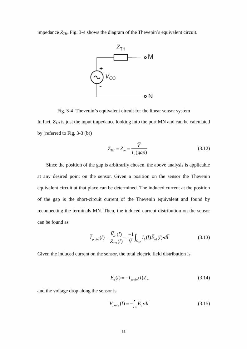
53

impedance ZTH. Fig. 3-4 shows the diagram of the Thevenin‘s equivalent circuit.

Fig. 3-4 Thevenin‘s equivalent circuit for the linear sensor system

In fact, ZTH is just the input impedance looking into the port MN and can be calculated

by (referred to Fig. 3-3 (b))

( )TH in

b

VZ Z

I gap (3.12)

Since the position of the gap is arbitrarily chosen, the above analysis is applicable

at any desired point on the sensor. Given a position on the sensor the Thevenin

equivalent circuit at that place can be determined. The induced current at the position

of the gap is the short-circuit current of the Thevenin equivalent and found by

reconnecting the terminals MN. Then, the induced current distribution on the sensor

can be found as

1

( ) 1( ) ( ) ( )

( ) AB

ocprobe b a

CTH

V lI l I l E l dl

Z l V

(3.13)

Given the induced current on the sensor, the total electric field distribution is

( ) ( )a probe wE l I l Z (3.14)

and the voltage drop along the sensor is

( )probe aC

V l E dl (3.15)

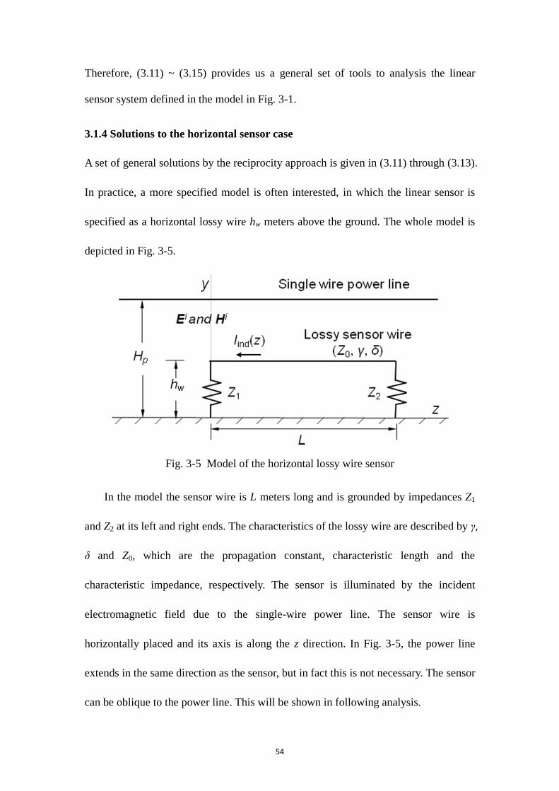
54

Therefore, (3.11) ~ (3.15) provides us a general set of tools to analysis the linear

sensor system defined in the model in Fig. 3-1.

3.1.4 Solutions to the horizontal sensor case

A set of general solutions by the reciprocity approach is given in (3.11) through (3.13).

In practice, a more specified model is often interested, in which the linear sensor is

specified as a horizontal lossy wire hw meters above the ground. The whole model is

depicted in Fig. 3-5.

Fig. 3-5 Model of the horizontal lossy wire sensor

In the model the sensor wire is L meters long and is grounded by impedances Z1

and Z2 at its left and right ends. The characteristics of the lossy wire are described by γ,

δ and Z0, which are the propagation constant, characteristic length and the

characteristic impedance, respectively. The sensor is illuminated by the incident

electromagnetic field due to the single-wire power line. The sensor wire is

horizontally placed and its axis is along the z direction. In Fig. 3-5, the power line

extends in the same direction as the sensor, but in fact this is not necessary. The sensor

can be oblique to the power line. This will be shown in following analysis.

55

From (3.13), the induced current at any point (0 < z < L) on the lossy wire can be

found as

0

0

0

1( ) ( ,0) ( , 0)

( , ) ( , )

( , ) ( , )

w

w

hi

ind t y

hi

t y

Li

t z w

I z I z E y z dyV

I z L E y z L dy

I z z E y h z dz

(3.16)

where ( , )tI z z is the current at position z’ on the lossy wire when it is driven by a

voltage source V at z’ = z, It(z, 0) and It(z, L) are the currents at z’ = 0 and z’ = L driven

by the same voltage source. ( , 0)i

yE y z is the y-component of the incident electric

field along y’ axis at z’ = 0, and ( , )i

yE y z L is the similar component at z’ = L.

( , )i

z wE y h z is the z-component of the incident electric field along z’ axis at y’ = hw.

It(z, z’) can be found by using the classical transmission line theory as

( ) 2 ( )

1 2 12

0 1 2

( , )2 1

z z z zz z L z z

t L

VI z z e e e e e

Z e

(3.17)

where 1 01

1 0

Z Z

Z Z

and 2 0

2

2 0

Z Z

Z Z

. Inserting (3.17) into (3.16), with some algebra

manipulations the induced current in (3.16) can be rewritten as

1 1 2 30

0

1 20 0

1( ) ( ) ( ) ( , ) ( ) ( ) ( , )

1( ) ( , 0) ( ) ( , )

sw sw

z Li i

ind z zz

h hi i

y y

I z A z B z E h z dz A z B z E h z dzZ D

A z E y z dy A z E y z L dyD

(3.18)

where

1 0 2( ) cosh sinhA z Z L z Z L z

2 0 1( ) cosh sinhA z Z z Z z

1 0 1( ) cosh sinhB z Z z Z z

3 0 2( ) cosh sinhB z Z L z Z L z

56

2

0 1 0 2 0 1 2cosh sinhD Z Z Z Z L Z Z Z L

Equations (3.16) and (3.18) are the solutions to the induced current of the

horizontal sensor model that are identical but of different form. According to these

results, the induced current can be determined at any point on the sensor if the

incident E fields at the position of the sensor are known. There is no requirement that

the relative position of the power line to the sensor wire is known as long as the

power line is horizontal and high enough (Hp >> hw). Thus the power line can be

parallel, oblique, or perpendicular to the sensor wire. The results in (3.16) and (3.18)

will be used in Chapter 4 and 5 for the cases of the perpendicular linear sensor and the

parallel linear sensor.

3.2 Approach by model of per-unit-length voltage and current sources

As shown, the reciprocity theorem can be used to find the induced current for the very

general model as depicted in Fig. 3-1. Now the model in Fig. 3-5 is considered and a

further assumption that the ground is perfect conductor is made. The new model is

shown in Fig. 3-6. For this problem a method based on classical transmission line

theory uses voltage-and-current sources to replace the external excitation.

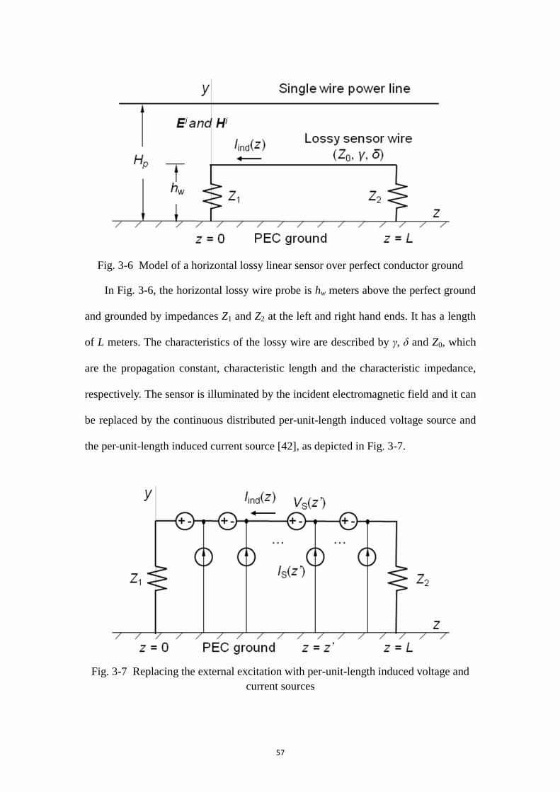
57

Fig. 3-6 Model of a horizontal lossy linear sensor over perfect conductor ground

In Fig. 3-6, the horizontal lossy wire probe is hw meters above the perfect ground

and grounded by impedances Z1 and Z2 at the left and right hand ends. It has a length

of L meters. The characteristics of the lossy wire are described by γ, δ and Z0, which

are the propagation constant, characteristic length and the characteristic impedance,

respectively. The sensor is illuminated by the incident electromagnetic field and it can

be replaced by the continuous distributed per-unit-length induced voltage source and

the per-unit-length induced current source [42], as depicted in Fig. 3-7.

Fig. 3-7 Replacing the external excitation with per-unit-length induced voltage and

current sources

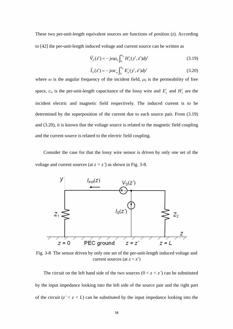
58

These two per-unit-length equivalent sources are functions of position (z). According

to [42] the per-unit-length induced voltage and current source can be written as

00

( ) ( , )wh

i

S xV z j H y z dy (3.19)

0( ) ( , )

whi

S w yI z j c E y z dy (3.20)

where ω is the angular frequency of the incident field, μ0 is the permeability of free

space, cw is the per-unit-length capacitance of the lossy wire and i

yE and i

xH are the

incident electric and magnetic field respectively. The induced current is to be

determined by the superposition of the current due to each source pair. From (3.19)

and (3.20), it is known that the voltage source is related to the magnetic field coupling

and the current source is related to the electric field coupling.

Consider the case for that the lossy wire sensor is driven by only one set of the

voltage and current sources (at z = z’) as shown in Fig. 3-8.

Fig. 3-8 The sensor driven by only one set of the per-unit-length induced voltage and

current sources (at z = z‘)

The circuit on the left hand side of the two sources (0 < z < z’) can be substituted

by the input impedance looking into the left side of the source pair and the right part

of the circuit (z’ < z < L) can be substituted by the input impedance looking into the

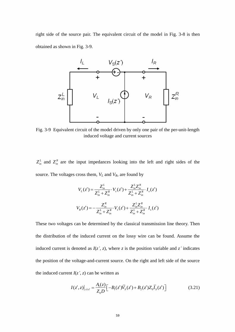
59

right side of the source pair. The equivalent circuit of the model in Fig. 3-8 is then

obtained as shown in Fig. 3-9.

Fig. 3-9 Equivalent circuit of the model driven by only one pair of the per-unit-length

induced voltage and current sources

L

inZ and R

inZ are the input impedances looking into the left and right sides of the

source. The voltages cross them, VL and VR, are found by

( ) ( ) ( )L L R

in in inL s sL R L R

in in in in

Z Z ZV z V z I z

Z Z Z Z

( ) ( ) ( )R L R

in in inR s sL R L R

in in in in

Z Z ZV z V z I z

Z Z Z Z

These two voltages can be determined by the classical transmission line theory. Then

the distribution of the induced current on the lossy wire can be found. Assume the

induced current is denoted as I(z’, z), where z is the position variable and z’ indicates

the position of the voltage-and-current source. On the right and left side of the source

the induced current I(z’, z) can be written as

11 2 0

0

( )( , ) ( ) ( ) ( ) ( )z z S S

A zI z z B z V z B z Z I z

Z D

(3.21)

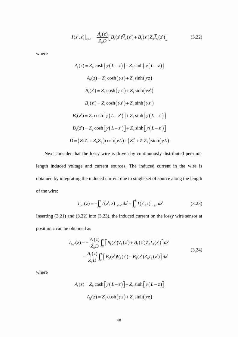
60

23 4 0

0

( )( , ) ( ) ( ) ( ) ( )z z S S

A zI z z B z V z B z Z I z

Z D

(3.22)

where

1 0 2( ) cosh sinhA z Z L z Z L z

2 0 1( ) cosh sinhA z Z z Z z

1 0 1( ) cosh sinhB z Z z Z z

2 1 0( ) cosh sinhB z Z z Z z

3 0 2( ) cosh sinhB z Z L z Z L z

4 2 0( ) cosh sinhB z Z L z Z L z

2

0 1 0 2 0 1 2cosh sinhD Z Z Z Z L Z Z Z L

Next consider that the lossy wire is driven by continuously distributed per-unit-

length induced voltage and current sources. The induced current in the wire is

obtained by integrating the induced current due to single set of source along the length

of the wire:

0( ) ( , ) ( , )

z L

ind z z z zz

I z I z z dz I z z dz (3.23)

Inserting (3.21) and (3.22) into (3.23), the induced current on the lossy wire sensor at

position z can be obtained as

11 2 0

00

23 4 0

0

( )( ) ( ) ( ) ( ) ( )

( )( ) ( ) ( ) ( )

z

ind S S

L

S Sz

A zI z B z V z B z Z I z dz

Z D

A zB z V z B z Z I z dz

Z D

(3.24)

where

1 0 2( ) cosh sinhA z Z L z Z L z

2 0 1( ) cosh sinhA z Z z Z z

61

1 0 1( ) cosh sinhB z Z z Z z

2 1 0( ) cosh sinhB z Z z Z z

3 0 2( ) cosh sinhB z Z L z Z L z

4 2 0( ) cosh sinhB z Z L z Z L z

2

0 1 0 2 0 1 2cosh sinhD Z Z Z Z L Z Z Z L

00

( ) ( , )wh

i

S xV z j H y z dy

0( ) ( , )

whi

S w yI z j c E y z dy

It appears that the results using the reciprocity approach for the induced current

shown in (3.16) and (3.18) are different from (3.24). But it is shown below in Section

3.3 that they are identical.

3.3 Relationship between the two approaches

In this section the relation between the result (3.16) derived using the reciprocity

approach and the result (3.24) using the per-unit-length-source approach is studied.

Since the reciprocity method is more general, the analysis will be started from (3.16).

First, consider the current distribution shown in (3.17). Replacing the exponential

functions in it by the hyperbolic sine and cosine functions results in

1 1

0

2 3

0

( ) ( ) 0

( , )

( ) ( )

t

VA z B z z z

Z DI z z

VA z B z z z L

Z D

(3.25)

where

1 0 2( ) cosh sinhA z Z L z Z L z

2 0 1( ) cosh sinhA z Z z Z z

62

1 0 1( ) cosh sinhB z Z z Z z

3 0 2( ) cosh sinhB z Z L z Z L z

2

0 1 0 2 0 1 2cosh sinhD Z Z Z Z L Z Z Z L

The derivative of this current with respect to z’ is found as

1 2

0

2 4

0

( ) ( ) 0( , )

( ) ( )

t

VA z B z z z

Z DI z z

VzA z B z z z L

Z D

(3.26)

where

2 1 0( ) cosh sinhB z Z z Z z

4 2 0( ) cosh sinhB z Z L z Z L z

Second, pulling the current out of the first two integrals of (3.16) results in

0

0

0

1( ) ( ,0) ( , 0)

( , ) ( , )

( , ) ( , )

w

w

hi

ind t y

hi

t y

Li

t z w

I z I z E y z dyV

I z L E y z L dy

I z z E y h z dz

(3.27)

Using the definitions of the per-unit-length current source (3.20) in (3.27) yields

1

( ,0) (0) ( , ) ( )1( ) t S t S

ind

w w

I z I I z L I LI z C

V j c j c

(3.28)

where

10

( , ) ( , )L

i

t z wC I z z E y h z dz .

Third, from the Maxwell‘s equation

0E j H

the x component of the H field can be obtained as

63

0

, ,,

i i

y zi

x

E y z E y zj H y z

z y

(3.29)

Integrating both sides of (3.29) with respect to y’ from 0 to hw and using the definition

of the per-unit-length voltage source (3.19) leads to

0

,, 0, ( )

w

ih yi i

z w z S

E y zE y h z E y z V z dy

z

(3.30)

If the assumption 0, 0i

zE y z is made (i.e., the ground is assumed to be perfect

conductor), (3.30) becomes

0

,, ( )

w

ih yi

z w S

E y zE y h z V z dy

z

(3.31)

Inserting (3.31) into the term C1 in (3.28) and using (3.25) result in

1 1 1 2 30

0

( ) ( ) ( ) ( ) ( ) ( )z L

S Sz

VC A z B z V z dz A z B z V z dz M

Z D (3.32)

where

0 0

,( , )

w

ih L y

t

E y zM I z z dz dy

z

If the inner integral of M is evaluated by parts, M becomes

0 0

( , ) ( ) ( ,0) (0) ( , ),

wh Lit S t S ty

w w

I z L I L I z I I z zM E y z dz dy

j c j c z

Then, by using (3.20), (3.26) and the fact that 0 wZ j c , the term M can be

rewritten as

1 2 0 2 4 00

0

( , ) ( ) ( ,0) (0)

( ) ( ) ( ) ( ) ( ) ( )

t S t S

w w

z L

S Sz

I z L I L I z IM

j c j c

VA z B z Z I z dz A z B z Z I z dz

Z D

(3.33)

Finally, combining (3.28), (3.32), and (3.33) gives the result for the induced

current in the form of per-unit-length sources as

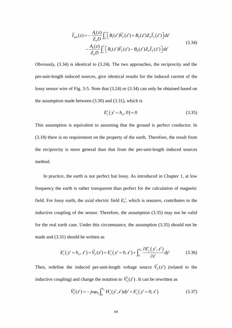
64

11 2 0

00

23 4 0

0

( )( ) ( ) ( ) ( ) ( )

( )( ) ( ) ( ) ( )

z

ind S S

L

S Sz

A zI z B z V z B z Z I z dz

Z D

A zB z V z B z Z I z dz

Z D

(3.34)

Obviously, (3.34) is identical to (3.24). The two approaches, the reciprocity and the

per-unit-length induced sources, give identical results for the induced current of the

lossy sensor wire of Fig. 3-5. Note that (3.24) or (3.34) can only be obtained based on

the assumption made between (3.30) and (3.31), which is

, 0 0i

z wE y h (3.35)

This assumption is equivalent to assuming that the ground is perfect conductor. In

(3.18) there is no requirement on the property of the earth. Therefore, the result from

the reciprocity is more general than that from the per-unit-length induced sources

method.

In practice, the earth is not perfect but lossy. As introduced in Chapter 1, at low

frequency the earth is rather transparent than perfect for the calculation of magnetic

field. For lossy earth, the axial electric field Ezi, which is nonzero, contributes to the

inductive coupling of the sensor. Therefore, the assumption (3.35) may not be valid

for the real earth case. Under this circumstance, the assumption (3.35) should not be

made and (3.31) should be written as

0

,, ( ) 0,

w

ih yi i

z w S z

E y zE y h z V z E y z dy

z

(3.36)

Then, redefine the induced per-unit-length voltage source ( )SV z (related to the

inductive coupling) and change the notation to ( )SV z . It can be rewritten as

00

( ) ( , ) 0,wh

i i

S x zV z j H y z dy E y z (3.37)

65

The effect of the lossy earth on the inductive coupling is embodied in axial incident

electric field added to (3.37). Using ( )SV z to substitute ( )SV z in (3.24) results in

11 2 0

00

23 4 0

0

( )( ) ( ) ( ) ( ) ( )

( )( ) ( ) ( ) ( )

z

ind S S

L

S Sz

A zI z B z V z B z Z I z dz

Z D

A zB z V z B z Z I z dz

Z D

(3.38)

where ( )SV z is defined by (3.37) and all the other variables or symbols are the same

as defined in (3.24). After the modification being made to ( )SV z , (3.38) is valid for

the case that the earth is lossy. It is unconditionally identical to the result by the

reciprocity method (3.18) and more general than (3.24). In Chapter 5, (3.38) will be

used for the analysis of the parallel linear sensor because for this kind of sensor the

inductive (magnetic) coupling is involved and the effect of the lossy earth on the

induced current cannot be ignored.

In [46] another approach using a model of the continuous distributed voltage

source is provided to formulate the induced current of a lossy transmission line which

is the analogue to the lossy sensor wire of Fig. 3-5. The result is also proved to be

identical to (3.34), which means that the three approaches validate each other.

Either the reciprocity method or the per-unit-length source method has its own

advantages and should be utilized in different situations. The reciprocity result, (3.16)

or (3.18), only involves the incident electric field. It can be use in the case that the

electric field is easy to find. The advantage of (3.24) is that the effects of the electric

and magnetic couplings are explicitly separated. Thus, when both of the electric and

magnetic coupling are involved (3.24) will be more helpful for analysis.

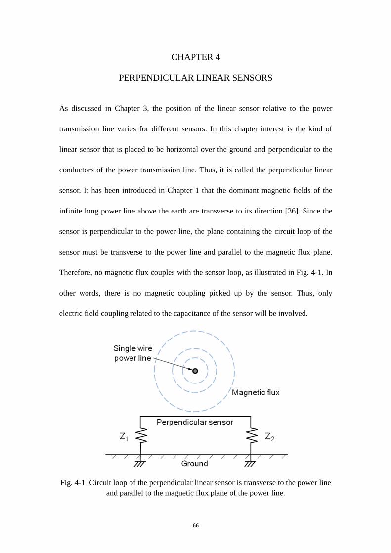
66

CHAPTER 4

PERPENDICULAR LINEAR SENSORS

As discussed in Chapter 3, the position of the linear sensor relative to the power

transmission line varies for different sensors. In this chapter interest is the kind of

linear sensor that is placed to be horizontal over the ground and perpendicular to the

conductors of the power transmission line. Thus, it is called the perpendicular linear

sensor. It has been introduced in Chapter 1 that the dominant magnetic fields of the

infinite long power line above the earth are transverse to its direction [36]. Since the

sensor is perpendicular to the power line, the plane containing the circuit loop of the

sensor must be transverse to the power line and parallel to the magnetic flux plane.

Therefore, no magnetic flux couples with the sensor loop, as illustrated in Fig. 4-1. In

other words, there is no magnetic coupling picked up by the sensor. Thus, only

electric field coupling related to the capacitance of the sensor will be involved.

Fig. 4-1 Circuit loop of the perpendicular linear sensor is transverse to the power line

and parallel to the magnetic flux plane of the power line.

67

The perpendicular linear sensor can be designed for monitoring the power line

sag, which may caused by either conductor heating or ice coating. Heating can

increase the line sag by weakening the tensile strength of the conductor and increasing

its length [47] – [49]. Ice coating on the power line elongates the conductor by

increasing the weight of it [50], [51]. The perpendicular linear sensor can also be

made to detect the negative/zero sequence mode of the power line voltage. In the

following sections, a model of the perpendicular sensor is first introduced and the

theory of how the sensor works is derived in 4.1. Again, the induced current of the

sensor under the excitation from the power line is the focus. Second, the effects of

different parameters, such as the length, height, resistance and capacitance of the

sensor wire, on the induced current are discussed in 4.2. Applications using the

perpendicular sensors in sag monitoring and negative mode detection are introduced

in 4.3.

4.1 Model and theories

A model of the perpendicular linear sensor system is shown in Fig. 4-2. In this model,

the sensor is a horizontal lossy wire, L meters long and hw meters above the ground.

The sensor wire is placed perpendicular to a single-wire power line, which is Hp

meters above the ground and energized by a voltage source of Vp (kV). As mentioned

before, for the perpendicular linear sensor only the electric coupling, i.e., the

transverse electric field, will be involved in analyzing the theory. Thus the ground is

assumed to be perfect electric conductor (PEC) because of the quasi-static

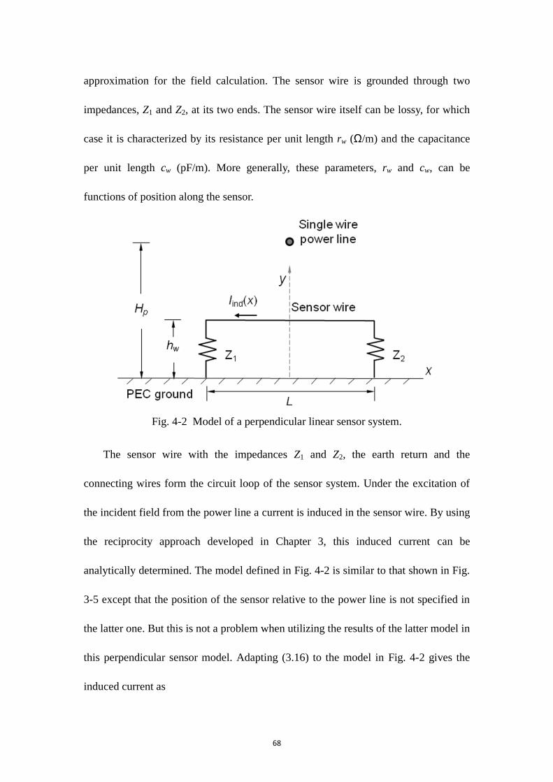
68

approximation for the field calculation. The sensor wire is grounded through two

impedances, Z1 and Z2, at its two ends. The sensor wire itself can be lossy, for which

case it is characterized by its resistance per unit length rw (Ω/m) and the capacitance

per unit length cw (pF/m). More generally, these parameters, rw and cw, can be

functions of position along the sensor.

Fig. 4-2 Model of a perpendicular linear sensor system.

The sensor wire with the impedances Z1 and Z2, the earth return and the

connecting wires form the circuit loop of the sensor system. Under the excitation of

the incident field from the power line a current is induced in the sensor wire. By using

the reciprocity approach developed in Chapter 3, this induced current can be

analytically determined. The model defined in Fig. 4-2 is similar to that shown in Fig.

3-5 except that the position of the sensor relative to the power line is not specified in

the latter one. But this is not a problem when utilizing the results of the latter model in

this perpendicular sensor model. Adapting (3.16) to the model in Fig. 4-2 gives the

induced current as

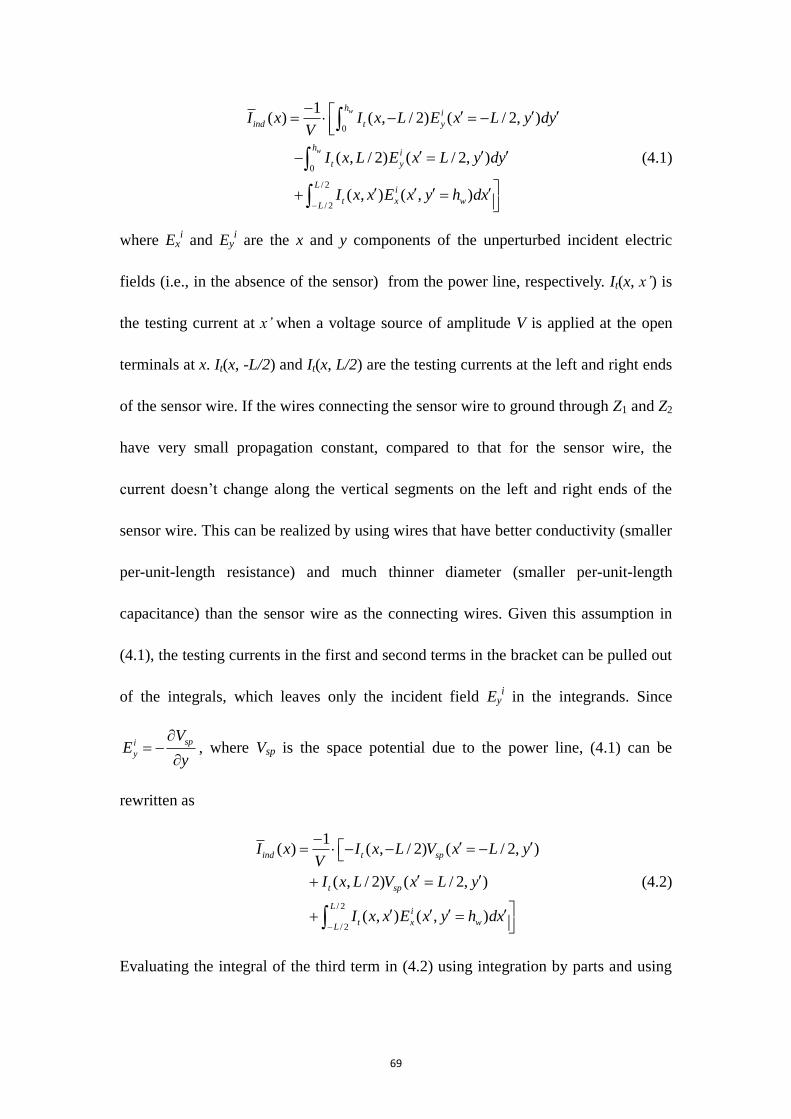
69

0

0

/ 2

/ 2

1( ) ( , / 2) ( / 2, )

( , / 2) ( / 2, )

( , ) ( , )

w

w

hi

ind t y

hi

t y

Li

t x wL

I x I x L E x L y dyV

I x L E x L y dy

I x x E x y h dx

(4.1)

where Exi and Ey

i are the x and y components of the unperturbed incident electric

fields (i.e., in the absence of the sensor) from the power line, respectively. It(x, x’) is

the testing current at x’ when a voltage source of amplitude V is applied at the open

terminals at x. It(x, -L/2) and It(x, L/2) are the testing currents at the left and right ends

of the sensor wire. If the wires connecting the sensor wire to ground through Z1 and Z2

have very small propagation constant, compared to that for the sensor wire, the

current doesn‘t change along the vertical segments on the left and right ends of the

sensor wire. This can be realized by using wires that have better conductivity (smaller

per-unit-length resistance) and much thinner diameter (smaller per-unit-length

capacitance) than the sensor wire as the connecting wires. Given this assumption in

(4.1), the testing currents in the first and second terms in the bracket can be pulled out

of the integrals, which leaves only the incident field Eyi in the integrands. Since

spi

y

VE

y

, where Vsp is the space potential due to the power line, (4.1) can be

rewritten as

/ 2

/ 2

1( ) ( , / 2) ( / 2, )

( , / 2) ( / 2, )

( , ) ( , )

ind t sp

t sp

Li

t x wL

I x I x L V x L yV

I x L V x L y

I x x E x y h dx

(4.2)

Evaluating the integral of the third term in (4.2) using integration by parts and using

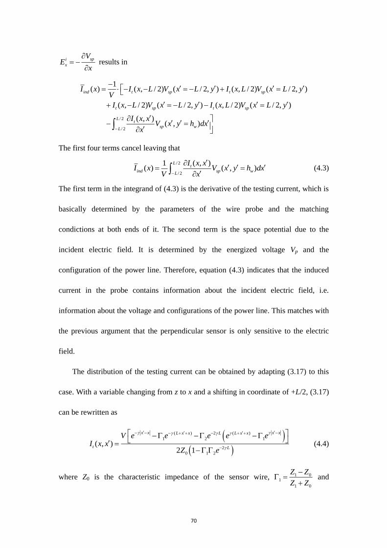
70

spi

x

VE

x

results in

/ 2

/ 2

1( ) ( , / 2) ( / 2, ) ( , / 2) ( / 2, )

( , / 2) ( / 2, ) ( , / 2) ( / 2, )

( , )( , )

ind t sp t sp

t sp t sp

Lt

sp wL

I x I x L V x L y I x L V x L yV

I x L V x L y I x L V x L y

I x xV x y h dx

x

The first four terms cancel leaving that

/ 2

/ 2

( , )1( ) ( , )

Lt

ind sp wL

I x xI x V x y h dx

V x

(4.3)

The first term in the integrand of (4.3) is the derivative of the testing current, which is

basically determined by the parameters of the wire probe and the matching

condictions at both ends of it. The second term is the space potential due to the

incident electric field. It is determined by the energized voltage Vp and the

configuration of the power line. Therefore, equation (4.3) indicates that the induced

current in the probe contains information about the incident electric field, i.e.

information about the voltage and configurations of the power line. This matches with

the previous argument that the perpendicular sensor is only sensitive to the electric

field.

The distribution of the testing current can be obtained by adapting (3.17) to this

case. With a variable changing from z to x and a shifting in coordinate of +L/2, (3.17)

can be rewritten as

( ) 2 ( )

1 2 1

2

0 1 2

( , )2 1

x x x xL x x L L x x

t L

V e e e e eI x x

Z e

(4.4)

where Z0 is the characteristic impedance of the sensor wire, 1 01

1 0

Z Z

Z Z

and

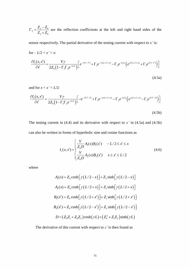
71

2 02

2 0

Z Z

Z Z

are the reflection coefficients at the left and right hand sides of the

sensor respectively. The partial derivative of the testing current with respect to x’ is:

for – L/2 < x’ < x:

( ) 2 ( )

1 2 12

0 1 2

( , )

2 1

x x x xL x x L L x xt

L

I x x Ve e e e e

x Z e

(4.5a)

and for x < x’ < L/2:

( ) 2 ( )

1 2 12

0 1 2

( , )

2 1

x x x xL x x L L x xt

L

I x x Ve e e e e

x Z e

(4.5b)

The testing current in (4.4) and its derivative with respect to x’ in (4.5a) and (4.5b)

can also be written in forms of hyperbolic sine and cosine functions as

1 1

0

2 3

0

( ) ( ) / 2

( , )

( ) ( ) / 2

t

VA x B x L x x

Z DI x x

VA x B x x x L

Z D

(4.6)

where

1 0 2( ) cosh / 2 sinh / 2A x Z L x Z L x

2 0 1( ) cosh / 2 sinh / 2A x Z L x Z L x

1 0 1( ) cosh / 2 sinh / 2B x Z L x Z L x

3 0 2( ) cosh / 2 sinh / 2B x Z L x Z L x

2

0 1 0 2 0 1 2cosh sinhD Z Z Z Z L Z Z Z L

The derivative of this current with respect to z’ is then found as

72

1 2

0

2 4

0

( ) ( ) / 2( , )

( ) ( ) / 2

t

VA x B x L x x

Z DI x x

VxA x B x x x L

Z D

(4.7)

where

2 1 0( ) cosh / 2 sinh / 2B x Z L x Z L x

4 2 0( ) cosh / 2 sinh / 2B x Z L x Z L x

By using (4.7), the induced current in (4.3) can be rewritten in the forms of hyperbolic

sine and cosine functions as

12

/ 20

/ 22

4

0

( )( ) ( ) ( , )

( )( ) ( , )

x

ind sp wL

L

sp wx

A xI x B x V x y h dx

Z D

A xB x V x y h dx

Z D

(4.8)

where A1(x), A2(x), B2(x’), B4(x’), and D are defined as before.

As previously discussed, the perpendicular sensor involves only electric field (i.e.,

capacitive) coupling, which is similar to that of the point probe introduced in Chapter

2. In fact, the model in Fig. 4-2 can reduce to a point probe if the sensor is assumed to

be very short and open circuited at one of its ends. Consider that the length of the

sensor L is short enough that |γL| << 1 and the sensor is opened at x = L/2 (equivalent

to setting Z2 = ∞). The model with these assumptions is shown in Fig. 4-3.

73

Fig. 4-3 A perpendicular linear sensor reduces to point probe when its length is very

short and is opened at one of its end (x = L/2 for this case).

For the hyperbolic sine and cosine functions, given |γL| << 1 it yields that

cosh 1u and sinh 0u

where |u| < L. With these approximations (4.7) reduces to

1

0 1 2

2

0 1 2

/ 2( )( , )

/ 2( )

t

VZL x x

Z Z ZI x x

VZxx x L

Z Z Z

(4.9)

The induced current can be rewritten as

/ 21 2

/ 20 1 2 0 1 2

( ) ( , ) ( , )( ) ( )

x L

ind sp w sp wL x

Z ZI x V x y h dx V x y h dx

Z Z Z Z Z Z

Since |γL| << 1, the space potential doesn‘t change much along the sensor wire and it

can be assumed constant over the whole length of the sensor wire. Then, it yields that

, / 2

1 2

0 1 2

( ) / 2 / 2( )

sp L

ind

VI x x L Z L x Z

Z Z Z

where Vsp,-L/2 is the space potential at (x = -L/2, y = hw) and chosen to represent the

space potential value over the sensor. Taking a further step by using the assumption

74

that Z2 = ∞ and the fact that γ / Z0 = jωcw (cw is the per-unit-length capacitance of the

sensor) the induced current now can be written as

, / 2( ) / 2 / 2 / 2ind w sp LI x j c L x V L x L (4.10)

Therefore, the induced current in the grounding wire at x = -L / 2 is found as

,( / 2) ( )ind w sp avgI L j c L V (4.11)

Equation (4.11) gives the same result as (2.8) since cwL is the self-capacitance of the

sensor. Therefore a perpendicular sensor can reduce to a point probe if the length of

the sensor is short (|γL| << 1).

As shown in (4.3) or (4.11) the perpendicular linear sensor collects information

about the value of the space potential of the power line in. Many factors affect this

average value and hence the induced current of the sensor. The sag of the power line

conductor is one among those factors because the space potential is strongly related to

the configurations of the power line conductor. A perpendicular linear sensor can be

designed as a line-sag monitor such that the change of the line sag is recognized by

measuring the induced current. The discussion of this part will be introduced in

section 4.2.

In a similar way, the perpendicular sensor provides information not only the

magnitude but also about the phase angle of the space potential. One example of an

application using the phase angle information is the use of the perpendicular sensor to

detect the negative and zero components in the power line voltage. If the single-wire

power line in Fig. 4-2 is replaced by a three-phase power line, any change of the

symmetrical components of the power line voltage will cause the profile of the phase

75

distribution of the incident space potential to change. The perpendicular sensor can be

designed to be sensitive to this phase change and used as a negative or zero sequence

voltage detector. The detailed analysis and discussion will be introduced in section 4.3.

4.2 Sag monitoring by perpendicular linear sensor

It has been qualitatively known from the previous discussion that the current induced

on the sensor wire depends on the characteristics of the power line. If, for example,

the quantitative relation between the induced current and the line sag can be analyzed,

it is possible to design and built a sag sensor using the perpendicular linear sensor. To

examine this possibility, computer simulations based on the models of a horizontal-

configured and a delta-configured three-phase power line were conducted.

4.2.1 Power line models and parameters

Consider the two power transmission lines, configurations of which are shown in Fig.

4-4 (a) and (b), respectively.

(a) Model A: 230 kV horizontal line (b) Model B: 500 kV delta line

Fig. 4-4 Geometries of the perpendicular wire sensor and two types of three-phase

power transmission line

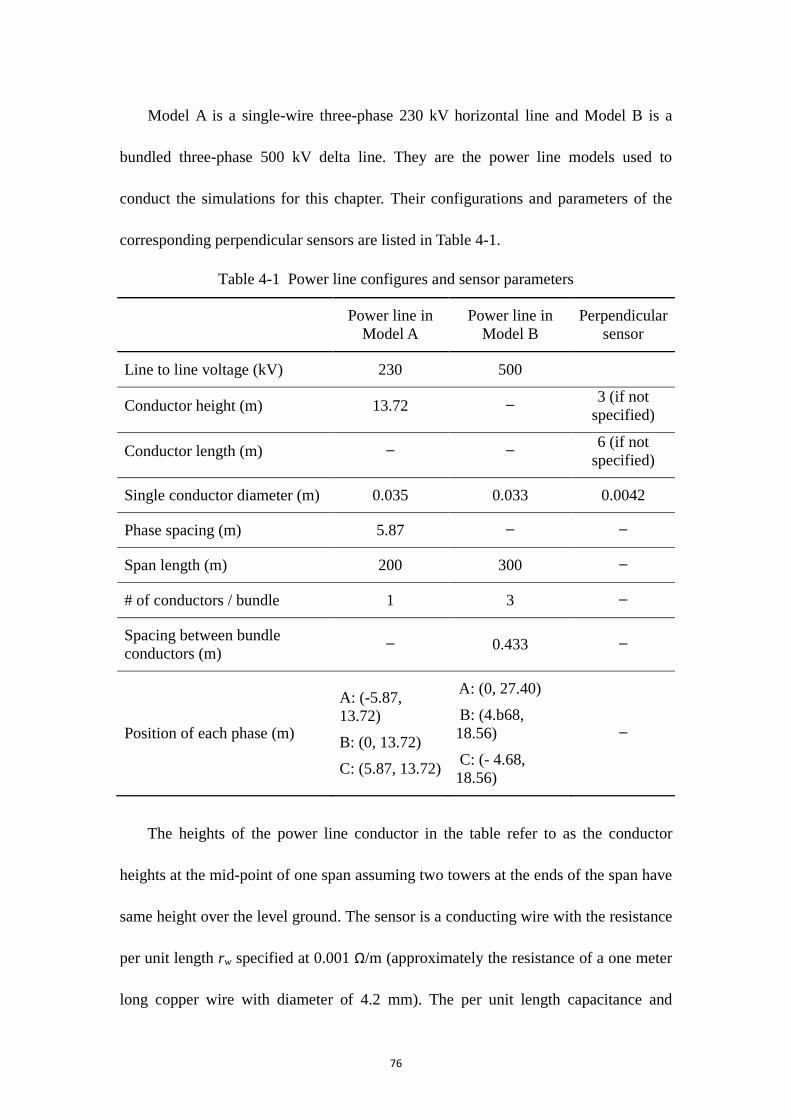
76

Model A is a single-wire three-phase 230 kV horizontal line and Model B is a

bundled three-phase 500 kV delta line. They are the power line models used to

conduct the simulations for this chapter. Their configurations and parameters of the

corresponding perpendicular sensors are listed in Table 4-1.

Table 4-1 Power line configures and sensor parameters

Power line in

Model A

Power line in

Model B

Perpendicular

sensor

Line to line voltage (kV) 230 500

Conductor height (m) 13.72 3 (if not

specified)

Conductor length (m) 6 (if not

specified)

Single conductor diameter (m) 0.035 0.033 0.0042

Phase spacing (m) 5.87

Span length (m) 200 300

# of conductors / bundle 1 3

Spacing between bundle

conductors (m) 0.433

Position of each phase (m)

A: (-5.87,

13.72)

B: (0, 13.72)

C: (5.87, 13.72)

A: (0, 27.40)

B: (4.b68,

18.56)

C: (- 4.68,

18.56)

The heights of the power line conductor in the table refer to as the conductor

heights at the mid-point of one span assuming two towers at the ends of the span have

same height over the level ground. The sensor is a conducting wire with the resistance

per unit length rw specified at 0.001 Ω/m (approximately the resistance of a one meter

long copper wire with diameter of 4.2 mm). The per unit length capacitance and

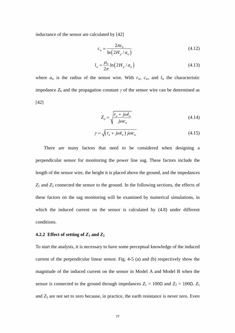
77

inductance of the sensor are calculated by [42]

02

ln 2 /w

p w

cH a

(4.12)

0 ln 2 /2

w p wl H a

(4.13)

where aw is the radius of the sensor wire. With rw, cw, and lw the characteristic

impedance Z0 and the propagation constant γ of the sensor wire can be determined as

[42]

0w w

w

r j lZ

j c

(4.14)

w w wr j l j c (4.15)

There are many factors that need to be considered when designing a

perpendicular sensor for monitoring the power line sag. These factors include the

length of the sensor wire, the height it is placed above the ground, and the impedances

Z1 and Z2 connected the sensor to the ground. In the following sections, the effects of

these factors on the sag monitoring will be examined by numerical simulations, in

which the induced current on the sensor is calculated by (4.8) under different

conditions.

4.2.2 Effect of setting of Z1 and Z2

To start the analysis, it is necessary to have some perceptual knowledge of the induced

current of the perpendicular linear sensor. Fig. 4-5 (a) and (b) respectively show the

magnitude of the induced current on the sensor in Model A and Model B when the

sensor is connected to the ground through impedances Z1 = 100Ω and Z2 = 100Ω. Z1

and Z2 are not set to zero because, in practice, the earth resistance is never zero. Even

78

when the sensor wire is directly connected to ground, the grounding resistance due to

the earth should still be taken account into the model. 100Ω is a reasonable value of

the grounding resistance. Fig. 4-6 shows the corresponding phase angles. The power

line sag is set to zero for these simulations. The results obtained by (4.8) are

represented by solid lines in the figures. To validate (4.8), a method [52] based on the

concept of superposition to calculate the induced current is used. The results are

presented in circles in the figures.

(a) Model A: 230 kV horizontal line (b) Model B: 500 kV delta line

Fig. 4-5 Magnitude of the induced current on the sensor when Z1 = 100Ω and Z2 =

100Ω

79

(a) Model A: 230 kV horizontal line (b) Model B: 500 kV delta line

Fig. 4-6 Phase angle of the induced current on the sensor when Z1 = 100Ω and Z2 =

100Ω

The magnitudes of the induced current of the two models are both symmetrical

about the midpoint of the sensor wire because of the symmetry of the models. The

space potential is received symmetrically on the left and right half of the sensor and

derivative of the testing current in (4.7) has symmetry about the midpoint of the

sensor. Given these facts, it seems qualitatively that the induced current at the

midpoint should always be zero if Z1 = Z2 because the current flows symmetrically

from the midpoint to the two ends of the sensor. But this is not true, as shown in Fig.

4-5. According to (4.3), the induced current is determined by the integration of the

derivative of the testing current multiplied by the space potential. From Fig. 2-5, the

phase angle distribution of the space potential is not mirrored by central vertical axis.

Consequently, the induced currents on the two halves of the sensor are not

symmetrical, in phase angle, about the central axis and don‘t always cancel each other.

Thus, the induced current at the midpoint can be nonzero.

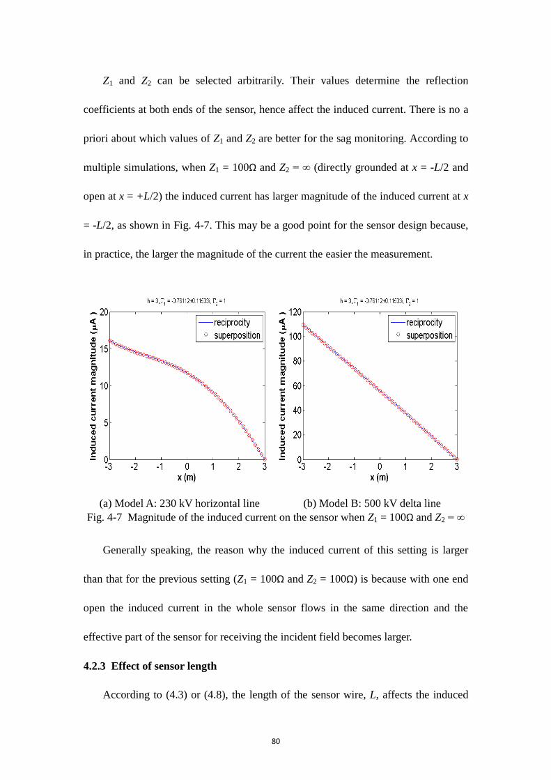
80

Z1 and Z2 can be selected arbitrarily. Their values determine the reflection

coefficients at both ends of the sensor, hence affect the induced current. There is no a

priori about which values of Z1 and Z2 are better for the sag monitoring. According to

multiple simulations, when Z1 = 100Ω and Z2 = ∞ (directly grounded at x = -L/2 and

open at x = +L/2) the induced current has larger magnitude of the induced current at x

= -L/2, as shown in Fig. 4-7. This may be a good point for the sensor design because,

in practice, the larger the magnitude of the current the easier the measurement.

(a) Model A: 230 kV horizontal line (b) Model B: 500 kV delta line

Fig. 4-7 Magnitude of the induced current on the sensor when Z1 = 100Ω and Z2 = ∞

Generally speaking, the reason why the induced current of this setting is larger

than that for the previous setting (Z1 = 100Ω and Z2 = 100Ω) is because with one end

open the induced current in the whole sensor flows in the same direction and the

effective part of the sensor for receiving the incident field becomes larger.

4.2.3 Effect of sensor length

According to (4.3) or (4.8), the length of the sensor wire, L, affects the induced

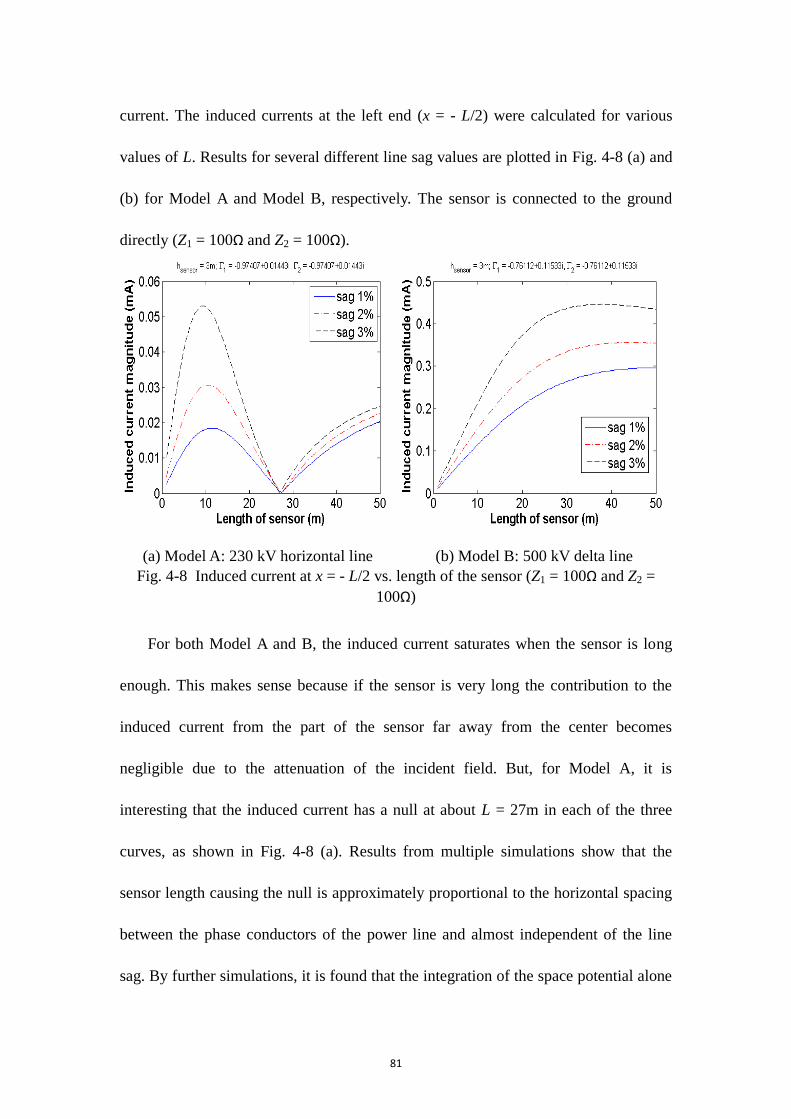
81

current. The induced currents at the left end (x = - L/2) were calculated for various

values of L. Results for several different line sag values are plotted in Fig. 4-8 (a) and

(b) for Model A and Model B, respectively. The sensor is connected to the ground

directly (Z1 = 100Ω and Z2 = 100Ω).

(a) Model A: 230 kV horizontal line (b) Model B: 500 kV delta line

Fig. 4-8 Induced current at x = - L/2 vs. length of the sensor (Z1 = 100Ω and Z2 =

100Ω)

For both Model A and B, the induced current saturates when the sensor is long

enough. This makes sense because if the sensor is very long the contribution to the

induced current from the part of the sensor far away from the center becomes

negligible due to the attenuation of the incident field. But, for Model A, it is

interesting that the induced current has a null at about L = 27m in each of the three

curves, as shown in Fig. 4-8 (a). Results from multiple simulations show that the

sensor length causing the null is approximately proportional to the horizontal spacing

between the phase conductors of the power line and almost independent of the line

sag. By further simulations, it is found that the integration of the space potential alone

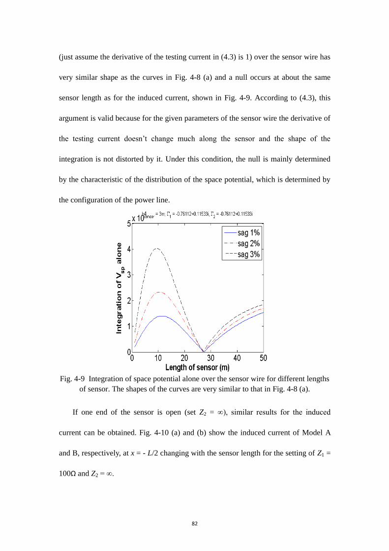
82

(just assume the derivative of the testing current in (4.3) is 1) over the sensor wire has

very similar shape as the curves in Fig. 4-8 (a) and a null occurs at about the same

sensor length as for the induced current, shown in Fig. 4-9. According to (4.3), this

argument is valid because for the given parameters of the sensor wire the derivative of

the testing current doesn‘t change much along the sensor and the shape of the

integration is not distorted by it. Under this condition, the null is mainly determined

by the characteristic of the distribution of the space potential, which is determined by

the configuration of the power line.

Fig. 4-9 Integration of space potential alone over the sensor wire for different lengths

of sensor. The shapes of the curves are very similar to that in Fig. 4-8 (a).

If one end of the sensor is open (set Z2 = ∞), similar results for the induced

current can be obtained. Fig. 4-10 (a) and (b) show the induced current of Model A

and B, respectively, at x = - L/2 changing with the sensor length for the setting of Z1 =

100Ω and Z2 = ∞.

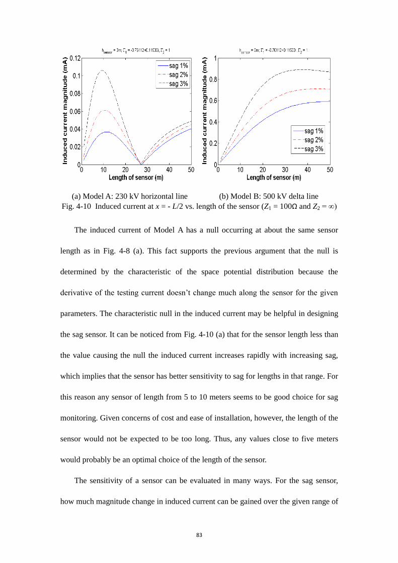
83

(a) Model A: 230 kV horizontal line (b) Model B: 500 kV delta line

Fig. 4-10 Induced current at x = - L/2 vs. length of the sensor (Z1 = 100Ω and Z2 = ∞)

The induced current of Model A has a null occurring at about the same sensor

length as in Fig. 4-8 (a). This fact supports the previous argument that the null is

determined by the characteristic of the space potential distribution because the

derivative of the testing current doesn‘t change much along the sensor for the given

parameters. The characteristic null in the induced current may be helpful in designing

the sag sensor. It can be noticed from Fig. 4-10 (a) that for the sensor length less than

the value causing the null the induced current increases rapidly with increasing sag,

which implies that the sensor has better sensitivity to sag for lengths in that range. For

this reason any sensor of length from 5 to 10 meters seems to be good choice for sag

monitoring. Given concerns of cost and ease of installation, however, the length of the

sensor would not be expected to be too long. Thus, any values close to five meters

would probably be an optimal choice of the length of the sensor.

The sensitivity of a sensor can be evaluated in many ways. For the sag sensor,

how much magnitude change in induced current can be gained over the given range of

84

sag values may be an important parameter. Hence, a factor Sc can be defined to show

the sensitivity of the sensor

max

min max min( )c

IS

I s s

(4.16)

where Imax and Imin are the maximum and minimum of induced current in the given

range of the line sag, smax and smin (in %) are the line sag values that cause Imax and

Imin, respectively. For a monotonically increasing current, Sc represents the steepness

of the curve. But for a current curve that has multiple peaks or valleys Sc may not be

the appropriate parameter.

4.2.4 Effect of sensor height

Obviously, the height of the sensor wire above the ground affects the induced

current. The higher the position of the probe the higher the magnitude of the space

potential, which in general will cause higher magnitude of induced current. Fig. 4-11

shows the results for Model A.

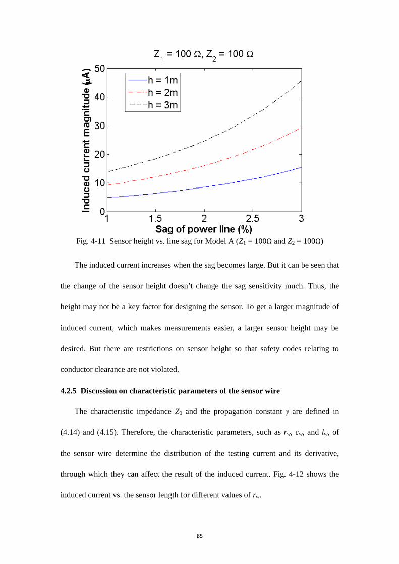
85

Fig. 4-11 Sensor height vs. line sag for Model A (Z1 = 100Ω and Z2 = 100Ω)

The induced current increases when the sag becomes large. But it can be seen that

the change of the sensor height doesn‘t change the sag sensitivity much. Thus, the

height may not be a key factor for designing the sensor. To get a larger magnitude of

induced current, which makes measurements easier, a larger sensor height may be

desired. But there are restrictions on sensor height so that safety codes relating to

conductor clearance are not violated.

4.2.5 Discussion on characteristic parameters of the sensor wire

The characteristic impedance Z0 and the propagation constant γ are defined in

(4.14) and (4.15). Therefore, the characteristic parameters, such as rw, cw, and lw, of

the sensor wire determine the distribution of the testing current and its derivative,

through which they can affect the result of the induced current. Fig. 4-12 shows the

induced current vs. the sensor length for different values of rw.

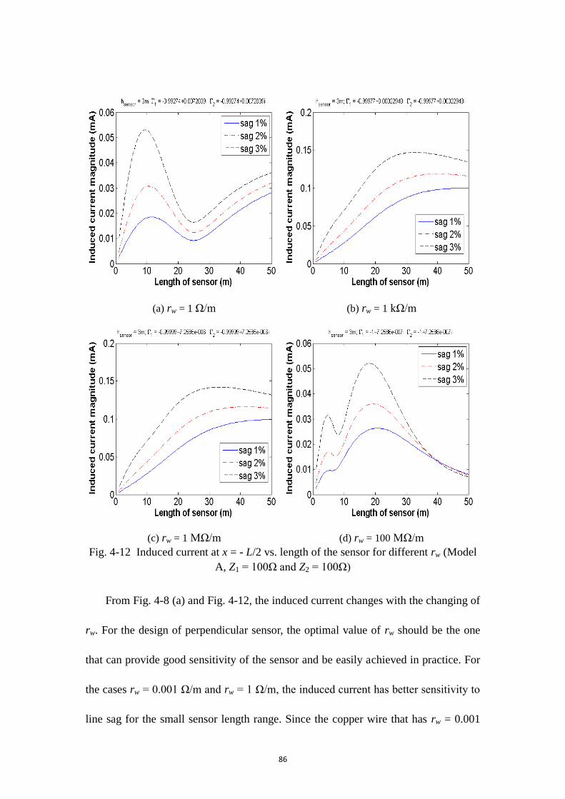
86

(a) rw = 1 Ω/m (b) rw = 1 kΩ/m

(c) rw = 1 MΩ/m (d) rw = 100 MΩ/m

Fig. 4-12 Induced current at x = - L/2 vs. length of the sensor for different rw (Model

A, Z1 = 100Ω and Z2 = 100Ω)

From Fig. 4-8 (a) and Fig. 4-12, the induced current changes with the changing of

rw. For the design of perpendicular sensor, the optimal value of rw should be the one

that can provide good sensitivity of the sensor and be easily achieved in practice. For

the cases rw = 0.001 Ω/m and rw = 1 Ω/m, the induced current has better sensitivity to

line sag for the small sensor length range. Since the copper wire that has rw = 0.001

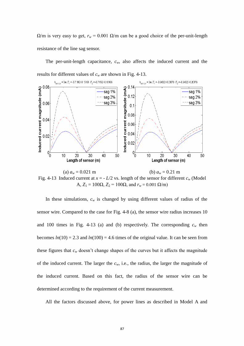
87

Ω/m is very easy to get, rw = 0.001 Ω/m can be a good choice of the per-unit-length

resistance of the line sag sensor.

The per-unit-length capacitance, cw, also affects the induced current and the

results for different values of cw are shown in Fig. 4-13.

(a) aw = 0.021 m (b) aw = 0.21 m

Fig. 4-13 Induced current at x = - L/2 vs. length of the sensor for different cw (Model

A, Z1 = 100Ω, Z2 = 100Ω, and rw = 0.001 Ω/m)

In these simulations, cw is changed by using different values of radius of the

sensor wire. Compared to the case for Fig. 4-8 (a), the sensor wire radius increases 10

and 100 times in Fig. 4-13 (a) and (b) respectively. The corresponding cw then

becomes ln(10) = 2.3 and ln(100) = 4.6 times of the original value. It can be seen from

these figures that cw doesn‘t change shapes of the curves but it affects the magnitude

of the induced current. The larger the cw, i.e., the radius, the larger the magnitude of

the induced current. Based on this fact, the radius of the sensor wire can be

determined according to the requirement of the current measurement.

All the factors discussed above, for power lines as described in Model A and

88

Model B, should be examined to determine optimal designs for building a good

perpendicular linear sensor for sag monitoring. A set of these parameters of the sensor

chosen based on above discussions is listed in Table 4-2 and makes a design of the

sensor used as power line sag monitor.

Table 4-2 Designs of the perpendicular linear sensor for sag monitoring

Sensor length, L 3 m

Sensor height, hw 2 m

Diameter of sensor, dw 4.2 mm

Resistance per unit length, rw 0.001 Ω/m

Setting of Z1 and Z2 Z1 = 100 Ω, Z2 = 100 Ω

4.3 Negative sequence mode detection by perpendicular linear sensor

Since a perpendicular linear sensor can provide some information about the space

potential, which is a phasor, it is possible to utilize the phase angle of the space

potential and design the sensor to detect the negative or zero sequence components of

the power line voltage. Assume the power line in Fig. 4-2 is a balanced three-phase

line with 120 degree phase shifts between each phase. As discussed in Chapter 2

(section 2.2), the negative and zero sequence components of the applied line voltage

can cause the profile of the phase angle distribution of the space potential to change,

which consequently causes the induced current in the sensor to change. Usually, the

presences of the negative and/or zero sequence voltage components are signs of the

abnormal conditions or faults occurring somewhere in the power system. If the

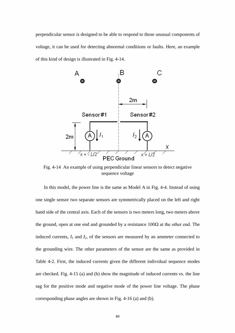
89

perpendicular sensor is designed to be able to respond to those unusual components of

voltage, it can be used for detecting abnormal conditions or faults. Here, an example

of this kind of design is illustrated in Fig. 4-14.

Fig. 4-14 An example of using perpendicular linear sensors to detect negative

sequence voltage

In this model, the power line is the same as Model A in Fig. 4-4. Instead of using

one single sensor two separate sensors are symmetrically placed on the left and right

hand side of the central axis. Each of the sensors is two meters long, two meters above

the ground, open at one end and grounded by a resistance 100Ω at the other end. The

induced currents, I1 and I2, of the sensors are measured by an ammeter connected to

the grounding wire. The other parameters of the sensor are the same as provided in

Table 4-2. First, the induced currents given the different individual sequence modes

are checked. Fig. 4-15 (a) and (b) show the magnitude of induced currents vs. the line

sag for the positive mode and negative mode of the power line voltage. The phase

corresponding phase angles are shown in Fig. 4-16 (a) and (b).

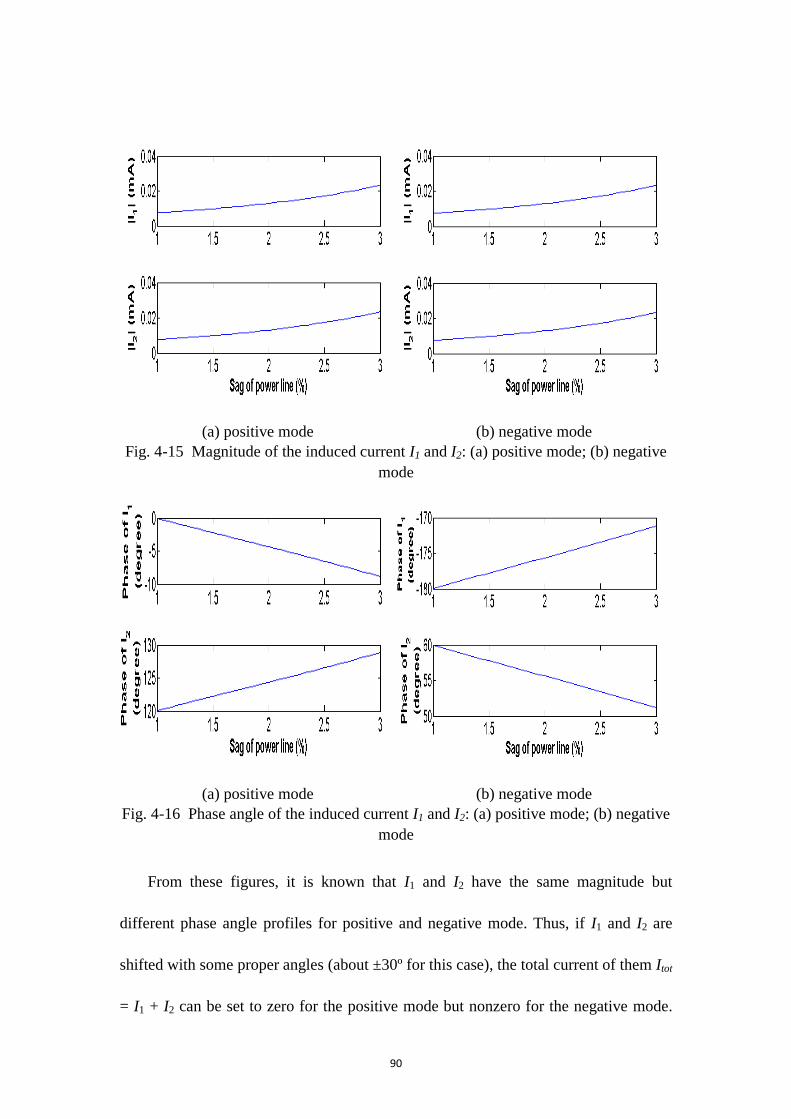
90

(a) positive mode (b) negative mode

Fig. 4-15 Magnitude of the induced current I1 and I2: (a) positive mode; (b) negative

mode

(a) positive mode (b) negative mode

Fig. 4-16 Phase angle of the induced current I1 and I2: (a) positive mode; (b) negative

mode

From these figures, it is known that I1 and I2 have the same magnitude but

different phase angle profiles for positive and negative mode. Thus, if I1 and I2 are

shifted with some proper angles (about ±30º for this case), the total current of them Itot

= I1 + I2 can be set to zero for the positive mode but nonzero for the negative mode.

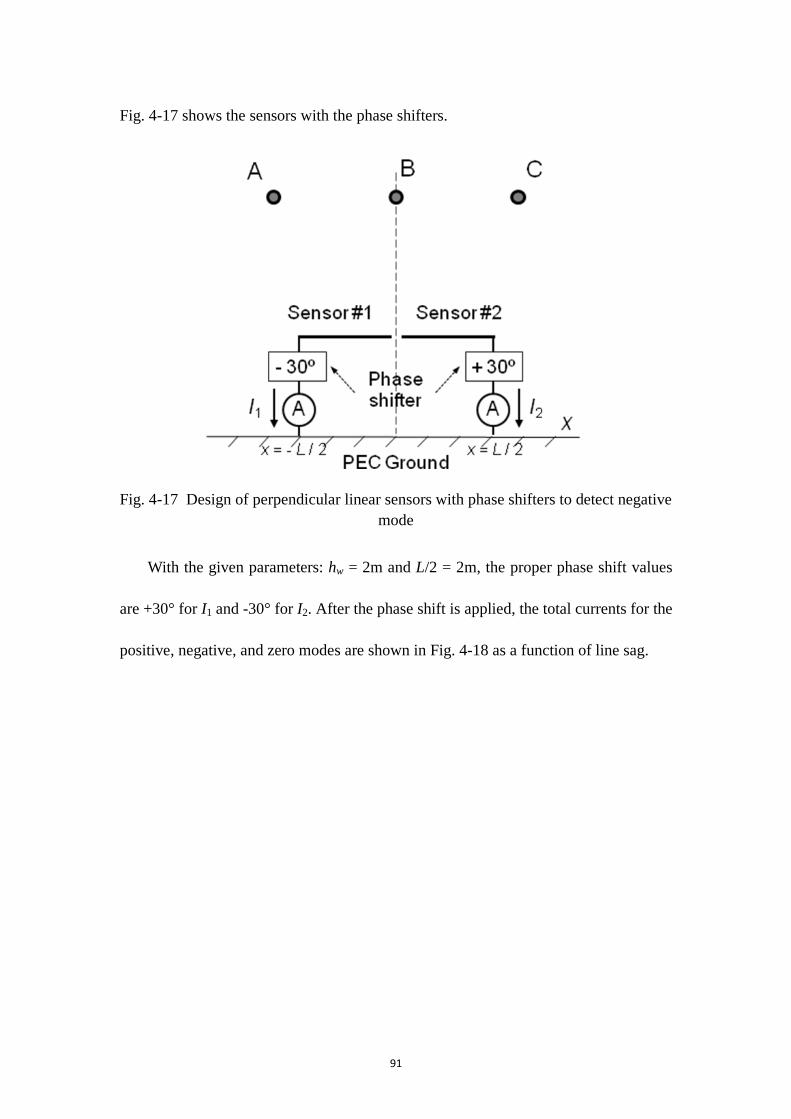
91

Fig. 4-17 shows the sensors with the phase shifters.

Fig. 4-17 Design of perpendicular linear sensors with phase shifters to detect negative

mode

With the given parameters: hw = 2m and L/2 = 2m, the proper phase shift values

are +30° for I1 and -30° for I2. After the phase shift is applied, the total currents for the

positive, negative, and zero modes are shown in Fig. 4-18 as a function of line sag.

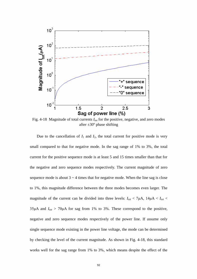
92

Fig. 4-18 Magnitude of total currents Itot for the positive, negative, and zero modes

after ±30º phase shifting

Due to the cancellation of I1 and I2, the total current for positive mode is very

small compared to that for negative mode. In the sag range of 1% to 3%, the total

current for the positive sequence mode is at least 5 and 15 times smaller than that for

the negative and zero sequence modes respectively. The current magnitude of zero

sequence mode is about 3 ~ 4 times that for negative mode. When the line sag is close

to 1%, this magnitude difference between the three modes becomes even larger. The

magnitude of the current can be divided into three levels: Itot < 7μA, 14μA < Itot <

35μA and Itot > 70μA for sag from 1% to 3%. These correspond to the positive,

negative and zero sequence modes respectively of the power line. If assume only

single sequence mode existing in the power line voltage, the mode can be determined

by checking the level of the current magnitude. As shown in Fig. 4-18, this standard

works well for the sag range from 1% to 3%, which means despite the effect of the

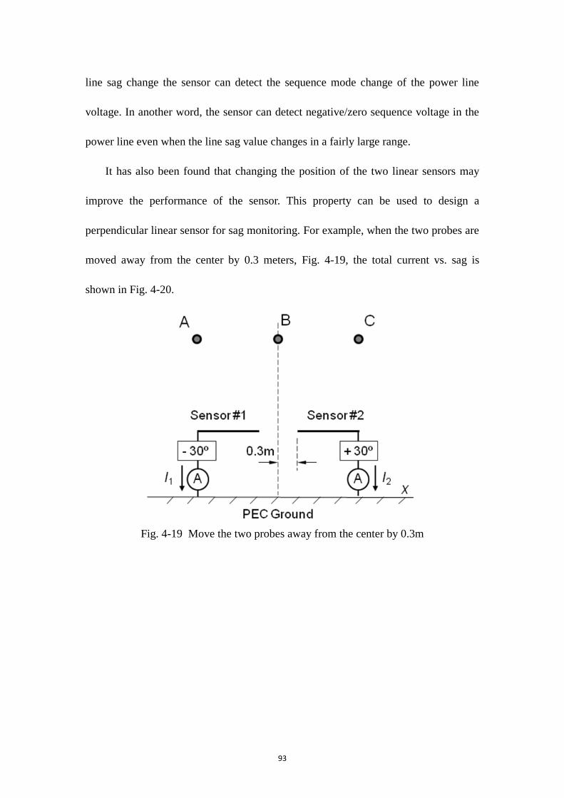
93

line sag change the sensor can detect the sequence mode change of the power line

voltage. In another word, the sensor can detect negative/zero sequence voltage in the

power line even when the line sag value changes in a fairly large range.

It has also been found that changing the position of the two linear sensors may

improve the performance of the sensor. This property can be used to design a

perpendicular linear sensor for sag monitoring. For example, when the two probes are

moved away from the center by 0.3 meters, Fig. 4-19, the total current vs. sag is

shown in Fig. 4-20.

Fig. 4-19 Move the two probes away from the center by 0.3m

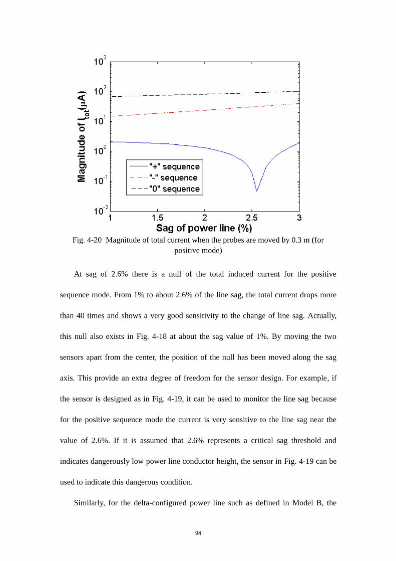
94

Fig. 4-20 Magnitude of total current when the probes are moved by 0.3 m (for

positive mode)

At sag of 2.6% there is a null of the total induced current for the positive

sequence mode. From 1% to about 2.6% of the line sag, the total current drops more

than 40 times and shows a very good sensitivity to the change of line sag. Actually,

this null also exists in Fig. 4-18 at about the sag value of 1%. By moving the two

sensors apart from the center, the position of the null has been moved along the sag

axis. This provide an extra degree of freedom for the sensor design. For example, if

the sensor is designed as in Fig. 4-19, it can be used to monitor the line sag because

for the positive sequence mode the current is very sensitive to the line sag near the

value of 2.6%. If it is assumed that 2.6% represents a critical sag threshold and

indicates dangerously low power line conductor height, the sensor in Fig. 4-19 can be

used to indicate this dangerous condition.

Similarly, for the delta-configured power line such as defined in Model B, the

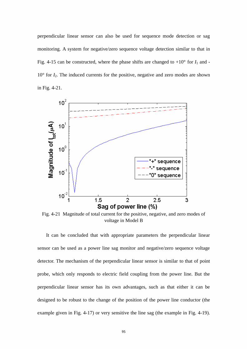
95

perpendicular linear sensor can also be used for sequence mode detection or sag

monitoring. A system for negative/zero sequence voltage detection similar to that in

Fig. 4-15 can be constructed, where the phase shifts are changed to +10° for I1 and -

10° for I2. The induced currents for the positive, negative and zero modes are shown

in Fig. 4-21.

Fig. 4-21 Magnitude of total current for the positive, negative, and zero modes of

voltage in Model B

It can be concluded that with appropriate parameters the perpendicular linear

sensor can be used as a power line sag monitor and negative/zero sequence voltage

detector. The mechanism of the perpendicular linear sensor is similar to that of point

probe, which only responds to electric field coupling from the power line. But the

perpendicular linear sensor has its own advantages, such as that either it can be

designed to be robust to the change of the position of the power line conductor (the

example given in Fig. 4-17) or very sensitive the line sag (the example in Fig. 4-19).

96

Additionally, since the perpendicular sensor has more complex structure than the

point probe it provides more degrees of freedom for the design.

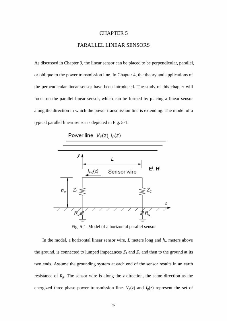
97

CHAPTER 5

PARALLEL LINEAR SENSORS

As discussed in Chapter 3, the linear sensor can be placed to be perpendicular, parallel,

or oblique to the power transmission line. In Chapter 4, the theory and applications of

the perpendicular linear sensor have been introduced. The study of this chapter will

focus on the parallel linear sensor, which can be formed by placing a linear sensor

along the direction in which the power transmission line is extending. The model of a

typical parallel linear sensor is depicted in Fig. 5-1.

Fig. 5-1 Model of a horizontal parallel sensor

In the model, a horizontal linear sensor wire, L meters long and hw meters above

the ground, is connected to lumped impedances Z1 and Z2 and then to the ground at its

two ends. Assume the grounding system at each end of the sensor results in an earth

resistance of Rg. The sensor wire is along the z direction, the same direction as the

energized three-phase power transmission line. Vp(z) and Ip(z) represent the set of

98

voltages and currents on the power line respectively. Under the excitation of the

incident electromagnetic fields (i.e., Ei and H

i, produced by the power line), there is a

current Iind(z) induced on the sensor wire.

The circuit loop formed by the sensor wire, the impedance Z1 and Z2, and the

earth return cuts the flux of the incident magnetic field, i.e., i

xH for this model.

Therefore, different from the point probe and the perpendicular linear sensor, the

parallel sensor receives the inductive (magnetic) coupling as well as the capacitive

(electric) coupling from the incident fields. The induced current on the sensor can be

decomposed into two components. One is related to the capacitive coupling, i.e. the

voltage on the power line, and the other is related to the inductive coupling, i.e. the

current on the power line. The differences in the nature of the capacitive and inductive

coupling bring more complexities but more possibilities to the design of the parallel

sensor. New functions other than those that can be realized using point probes or

perpendicular sensors are possible. One good example is the directional coupler for

detecting the traveling waves on the power line, which will be introduced in the

following sections.

5.1 Directional coupler

A parallel linear sensor can be designed to operate as a directional coupler for power

transmission lines (i.e., detecting forward and backward traveling wave amplitudes on

the lines). The directional coupler is often used in microwave circuits and one

definition of it is given as ―a device that couples a secondary system only to a wave

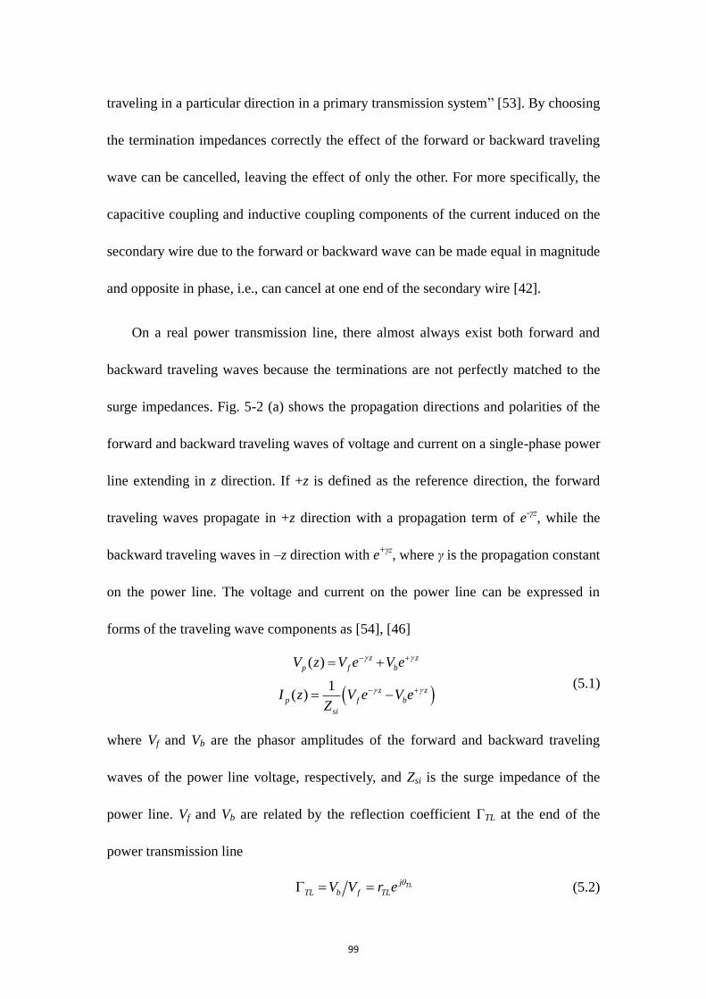
99

traveling in a particular direction in a primary transmission system‖ [53]. By choosing

the termination impedances correctly the effect of the forward or backward traveling

wave can be cancelled, leaving the effect of only the other. For more specifically, the

capacitive coupling and inductive coupling components of the current induced on the

secondary wire due to the forward or backward wave can be made equal in magnitude

and opposite in phase, i.e., can cancel at one end of the secondary wire [42].

On a real power transmission line, there almost always exist both forward and

backward traveling waves because the terminations are not perfectly matched to the

surge impedances. Fig. 5-2 (a) shows the propagation directions and polarities of the

forward and backward traveling waves of voltage and current on a single-phase power

line extending in z direction. If +z is defined as the reference direction, the forward

traveling waves propagate in +z direction with a propagation term of e-γz

, while the

backward traveling waves in –z direction with e+γz

, where γ is the propagation constant

on the power line. The voltage and current on the power line can be expressed in

forms of the traveling wave components as [54], [46]

( )

1( )

z z

p f b

z z

p f b

si

V z V e V e

I z V e V eZ

(5.1)

where Vf and Vb are the phasor amplitudes of the forward and backward traveling

waves of the power line voltage, respectively, and Zsi is the surge impedance of the

power line. Vf and Vb are related by the reflection coefficient ΓTL at the end of the

power transmission line

TLj

TL b f TLV V r e

(5.2)

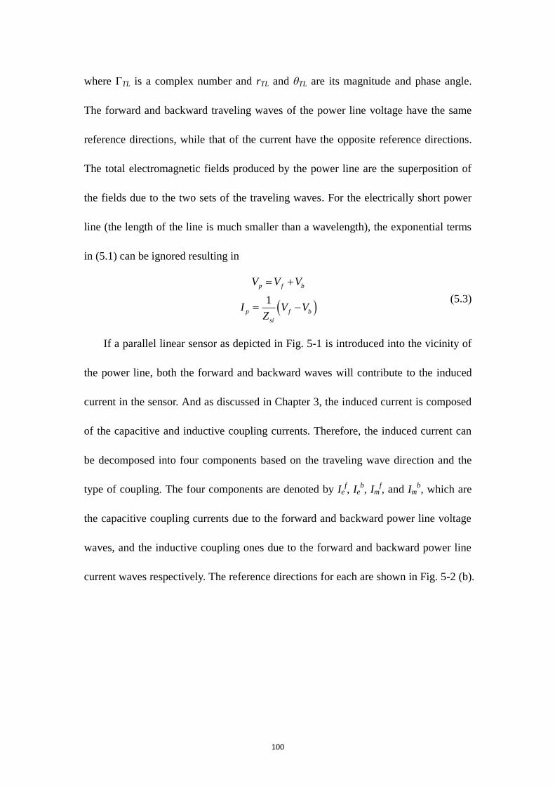
100

where ΓTL is a complex number and rTL and θTL are its magnitude and phase angle.

The forward and backward traveling waves of the power line voltage have the same

reference directions, while that of the current have the opposite reference directions.

The total electromagnetic fields produced by the power line are the superposition of

the fields due to the two sets of the traveling waves. For the electrically short power

line (the length of the line is much smaller than a wavelength), the exponential terms

in (5.1) can be ignored resulting in

1

p f b

p f b

si

V V V

I V VZ

(5.3)

If a parallel linear sensor as depicted in Fig. 5-1 is introduced into the vicinity of

the power line, both the forward and backward waves will contribute to the induced

current in the sensor. And as discussed in Chapter 3, the induced current is composed

of the capacitive and inductive coupling currents. Therefore, the induced current can

be decomposed into four components based on the traveling wave direction and the

type of coupling. The four components are denoted by Ief, Ie

b, Im

f, and Im

b, which are

the capacitive coupling currents due to the forward and backward power line voltage

waves, and the inductive coupling ones due to the forward and backward power line

current waves respectively. The reference directions for each are shown in Fig. 5-2 (b).

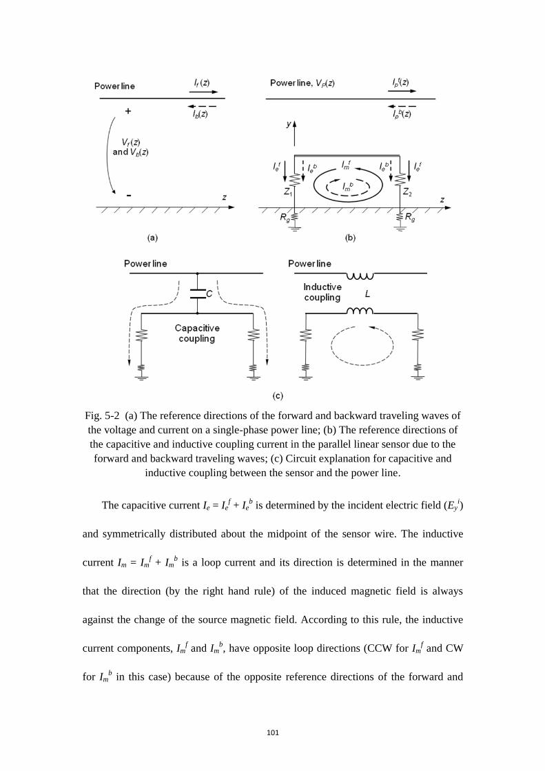
101

Fig. 5-2 (a) The reference directions of the forward and backward traveling waves of

the voltage and current on a single-phase power line; (b) The reference directions of

the capacitive and inductive coupling current in the parallel linear sensor due to the

forward and backward traveling waves; (c) Circuit explanation for capacitive and

inductive coupling between the sensor and the power line.

The capacitive current Ie = Ief + Ie

b is determined by the incident electric field (Ey

i)

and symmetrically distributed about the midpoint of the sensor wire. The inductive

current Im = Imf + Im

b is a loop current and its direction is determined in the manner

that the direction (by the right hand rule) of the induced magnetic field is always

against the change of the source magnetic field. According to this rule, the inductive

current components, Imf and Im

b, have opposite loop directions (CCW for Im

f and CW

for Imb in this case) because of the opposite reference directions of the forward and

102

backward traveling waves of power line current. The equivalent circuit explanation

for the capacitive and inductive coupling, as shown in Fig. 5-2 (c), is helpful for

understanding the direction of each component of the induced current.

Whether being induced by the forward or backward traveling waves on the power

line, the capacitive and inductive currents have same signs at one end of the sensor

wire and opposite signs at the other end. As shown in Fig. 5-2 (b), for the case of

forward traveling waves, Ief has the same sign as Im

f at the left end of the sensor (at Z1),

but has opposite sign at the right end (Z2). Based on the analysis of Chapter 3, by

carefully choosing Z1 and Z2 it can be realized that Ief = - Im

f at the right end of the

sensor wire. In other words, the induced current due to the forward wave on the power

line can be set to zero in the vertical branch on the right side of Fig. 5-2 (b). And the

induced current measured in that branch is then only determined by the backward

wave on the power line. Similarly, the induced current due to the backward wave can

be set to zero in the left branch and that due to the forward waves is measured in there.

This is basic mechanism for the parallel linear sensor to work as a directional coupler

for the power line. The voltage at one end represents the forward wave amplitude

while the voltage at the other end represents the backward wave amplitude.

The theory of the linear sensor has been introduced in Chapter 3. The induced

current distribution on a parallel linear sensor can be determined by the reciprocity

method and the result is shown in (3.18). But, here, it is more convenient to use the

result in (3.38), which is identical to (3.18), because the capacitive and inductive

components of the induced current are separated in (3.38) and it helps to obtain

103

insight into how the directional coupler works to detect the forward or backward

traveling waves. Here, (3.38) is repeated and the equation number is changed to (5.4)

11 2 0

00

23 4 0

0

( )( ) ( ) ( ) ( ) ( )

( )( ) ( ) ( ) ( )

z

ind S S

L

S Sz

A zI z B z V z B z Z I z dz

Z D

A zB z V z B z Z I z dz

Z D

(5.4)

where L is the length of the sensor wire and

1 0 2( ) cosh sinhA z Z L z Z L z

2 0 1( ) cosh sinhA z Z z Z z

1 0 1( ) cosh sinhB z Z z Z z

2 1 0( ) cosh sinhB z Z z Z z

3 0 2( ) cosh sinhB z Z L z Z L z

4 2 0( ) cosh sinhB z Z L z Z L z

2

0 1 0 2 0 1 2cosh sinhD Z Z Z Z L Z Z Z L

0( ) ( , )

whi

S w yI z j c E y z dy

00

( ) ( , ) 0,wh

i i

S x zV z j H y z dy E y z

The induced per-unit-length voltage source is modified by adding the axial

electric field on the air-earth interface to take care of the case of the lossy earth. In

(5.4), the terms containing IS are related to the capacitive coupling and that containing

VS are related to the inductive coupling. Then, (5.4) can be rewritten as

( ) ( ) ( )ind e mI z I z I z (5.5)

where

1 22 0 4 0

00 0

( ) ( )( ) ( ) ( ) ( ) ( )

z L

e S Sz

A z A zI z B z Z I z dz B z Z I z dz

Z D Z D (5.6)

104

1 21 3

00 0

( ) ( )( ) ( ) ( ) ( ) ( )

z L

m S Sz

A z A zI z B z V z dz B z V z dz

Z D Z D (5.7)

The induced current at Z1 (the left end of the sensor, z = 0), I1, is found as

1 1 1(0)ind e mI I I I (5.8)

where 21 4 0

00

(0)( ) ( )

L

e S

AI B z Z I z dz

Z D and 2

1 30

0

(0)( ) ( )

L

m S

AI B z V z dz

Z D . And the

induced current at Z2 (the right end of the sensor, z = L), I2, is

2 2 2( )ind e mI I L I I (5.9)

where 12 2 0

00

( )( ) ( )

L

e S

A LI B z Z I z dz

Z D and 1

2 10

0

( )( ) ( )

L

m S

A LI B z V z dz

Z D . It can be

observed from (5.8) and (5.9) that the induced current at one end of the sensor is

related only to the lumped impedance at the other end of the sensor, i.e., I1 is only

related to Z2 and I2 is only related to Z1.

First, let I2 = 0 in (5.9), resulting in Ie2 = - Im2, and Z1 can be solved by

00

1 0

00

cosh ( ) sinh ( )

sinh ( ) cosh ( )

L

S S

gL

S S

z V z z Z I z dzZ Z R

z V z z Z I z dz

(5.10)

Equation (5.10) gives the solution of Z1 which leads to zero induced current at Z2 (I2 =

0). Similarly, the value of Z2 causing zero induced current at Z1 can be determined by

letting I1 = 0 and solving (5.8)

00

2 0

00

cosh ( ) sinh ( )

sinh ( ) cosh ( )

L

S S

gL

S S

L z V z L z Z I z dzZ Z R

L z V z L z Z I z dz

(5.11)

Generally, for specified set of power line voltage and current, Z1 and Z2 are

different, which means that single impedance value cannot cause zero induced current

105

at both sides of the sensor wire. In (5.10) and (5.11), the earth resistance of the

grounding system is subtracted from the lumped impedance of Z1 and Z2. In the above

derivation, the conditions of the traveling waves on the power line have not been

mentioned. There could be pure forward or backward traveling waves, or some

combination of them on the power line. The effects of the power line voltage and

current are implicitly included in the induced per-unit-length sources IS and V’S. From

the polarities shown in Fig. 5-2 (b), if pure forward traveling waves are assumed on

the power line, I2 is zero if Z1 is determined by using (5.10). The result is rewritten as

00

1 0

00

cosh ( ) sinh ( )

sinh ( ) cosh ( )

Lf f

S Sf

gLf f

S S

z V z z Z I z dzZ Z R

z V z z Z I z dz

(5.12)

where the notations of the per-unit-length sources SI and V have been changed to

f

SI and f

SV respectively to represent the case of pure forward waves on the power

line. In the other hand, if assume pure backward traveling waves are assumed on the

power line, I1 can be set to zero when Z2 is determined by using (5.11). The result is

rewritten as

00

2 0

00

cosh ( ) sinh ( )

sinh ( ) cosh ( )

Lb b

S Sb

gLb b

S S

L z V z L z Z I z dzZ Z R

L z V z L z Z I z dz

(5.13)

where b

SI and b

SV are used to represent the case of pure backward waves on the

power line.

Now, consider the case in which the power line voltage and current contain both

the forward and backward traveling waves. Assume the values of Z1 and Z2 have been

determined by using (5.12) and (5.13).

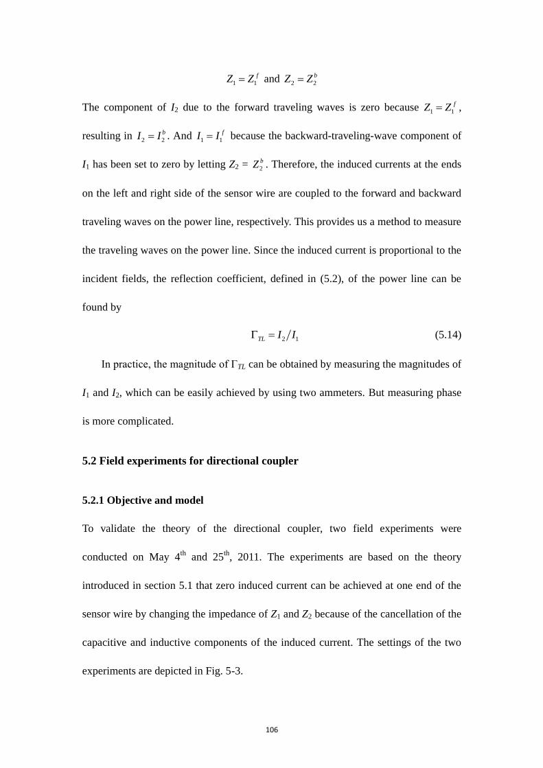
106

1 1

fZ Z and 2 2

bZ Z

The component of I2 due to the forward traveling waves is zero because 1 1

fZ Z ,

resulting in 2 2

bI I . And 1 1

fI I because the backward-traveling-wave component of

I1 has been set to zero by letting Z2 = 2

bZ . Therefore, the induced currents at the ends

on the left and right side of the sensor wire are coupled to the forward and backward

traveling waves on the power line, respectively. This provides us a method to measure

the traveling waves on the power line. Since the induced current is proportional to the

incident fields, the reflection coefficient, defined in (5.2), of the power line can be

found by

2 1TL I I (5.14)

In practice, the magnitude of ΓTL can be obtained by measuring the magnitudes of

I1 and I2, which can be easily achieved by using two ammeters. But measuring phase

is more complicated.

5.2 Field experiments for directional coupler

5.2.1 Objective and model

To validate the theory of the directional coupler, two field experiments were

conducted on May 4th

and 25th

, 2011. The experiments are based on the theory

introduced in section 5.1 that zero induced current can be achieved at one end of the

sensor wire by changing the impedance of Z1 and Z2 because of the cancellation of the

capacitive and inductive components of the induced current. The settings of the two

experiments are depicted in Fig. 5-3.

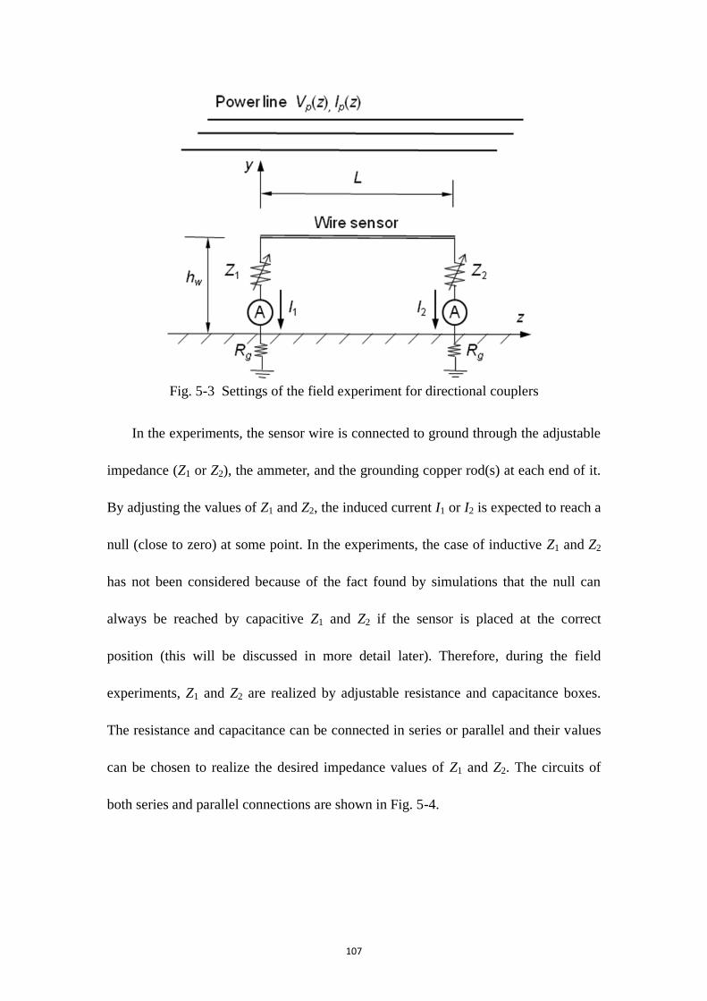
107

Fig. 5-3 Settings of the field experiment for directional couplers

In the experiments, the sensor wire is connected to ground through the adjustable

impedance (Z1 or Z2), the ammeter, and the grounding copper rod(s) at each end of it.

By adjusting the values of Z1 and Z2, the induced current I1 or I2 is expected to reach a

null (close to zero) at some point. In the experiments, the case of inductive Z1 and Z2

has not been considered because of the fact found by simulations that the null can

always be reached by capacitive Z1 and Z2 if the sensor is placed at the correct

position (this will be discussed in more detail later). Therefore, during the field

experiments, Z1 and Z2 are realized by adjustable resistance and capacitance boxes.

The resistance and capacitance can be connected in series or parallel and their values

can be chosen to realize the desired impedance values of Z1 and Z2. The circuits of

both series and parallel connections are shown in Fig. 5-4.

108

Fig. 5-4 Resistor and capacitor connected in series and parallel

For series connection, given the capacitive Z1 or Z2 calculated from (5.10) or

(5.11), the values of the resistance and capacitance to be chosen are found by

1

6

1

Re( ) ( )

10(μF)

Im( )

gR Z R

CZ

(5.a12)

For parallel connection, they are found by solving the equation set

1 2

2

1 2

Re( ) 01

Im( ) 01

g

RZ R

RC

R CZ

RC

(5.a13)

where R is in Ω and C is in F. For the record, if Z1 is inductive, the resistance and

inductance in series connection can be found by

1

1

Re( ) ( )

Im( )(H)

gR Z R

ZL

(5.a14)

and for parallel connection they can be found by

2

1

1

1

22

1 1

1

Im( )Re( ) ( )

Re( )

Im( ) Re( ) (H)

Im( )

g

g

g

ZR Z R

Z R

Z Z RL

Z

(5.a15)

109

Conducting the experiments is not as straight forward as deriving the theory.

Since the separate traveling wave amplitudes on the power line to be tested are not

known (equivalent to not knowing the reflection coefficient on the power line or the

relative phase difference between the voltage and current on the power line), the

values of Z1 and Z2, which can cause the null of the induced current, cannot be

calculated beforehand. The only available information of the voltage and current on

the power line is their magnitudes. This increases the unpredictability of the

experiment and the difficulties in finding the null of the induced current. Details will

be introduced in following sections.

5.2.2 Settings and preparations of experiment

The Benewah - Moscow 230kV power transmission line, owned by the Avista

Utilities, was the power line tested. This line is single circuit with horizontal

configuration. The experiment site is on land owned by John Salsbury and used with

permission. The land is about three miles east to Moscow, ID and two miles north of

the Moscow substation. It is on the intersection point of the Benewah - Moscow line

with Robinson Park Rd. The experiment site was chosen to be at the midpoint of the

north-south oriented span crossing the Robinson Park Rd. The span length is about

150m and the ground under that span is very flat, which is ideal for conducting the

experiments. In Fig. 5-5, photographs of the experiment settings taken from the

experiment site are shown.

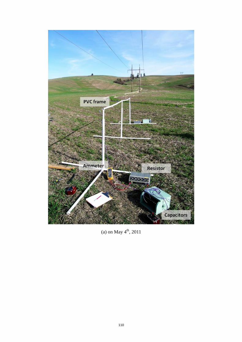
110

(a) on May 4th

, 2011

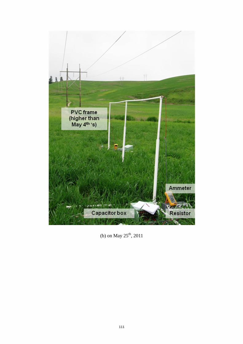
111

(b) on May 25th

, 2011

112

(c) closer look of the resistor box, capacitor box, and ammeter

Fig. 5-5 Experiment site and settings of the experiments for directional couplers.

On May 4th

, when conducting the experiment, the voltage of the power line was

242kV and the average phase current was 221A. The parameters of the line

configuration are not known, but they can be estimated by some indirect methods

such as measuring the electric field produced by the line to estimate the height and

spacing of the line conductors. For this reason, the electric field in the vertical

direction (Ey) was first measured at a height of one meter above the ground and the

height and spacing of the line conductors was estimated by matching the measured

data of Ey with the theoretical calculation. The comparison of results of measured and

calculated Ey are shown in Fig. 5-6. After multiple calculation attempts, the conductor

height at mid-span of 10.4m (34ft) and spacing of 6m was found to give the best

match with the measured data. Thus, these two values will be used as the parameters

of the power line.

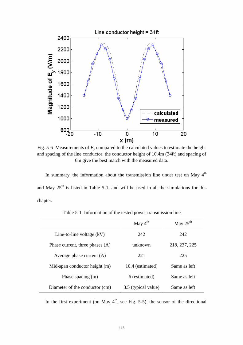
113

Fig. 5-6 Measurements of Ey compared to the calculated values to estimate the height

and spacing of the line conductor, the conductor height of 10.4m (34ft) and spacing of

6m give the best match with the measured data.

In summary, the information about the transmission line under test on May 4th

and May 25th

is listed in Table 5-1, and will be used in all the simulations for this

chapter.

Table 5-1 Information of the tested power transmission line

May 4th

May 25th

Line-to-line voltage (kV) 242 242

Phase current, three phases (A) unknown 218, 237, 225

Average phase current (A) 221 225

Mid-span conductor height (m) 10.4 (estimated) Same as left

Phase spacing (m) 6 (estimated) Same as left

Diameter of the conductor (cm) 3.5 (typical value) Same as left

In the first experiment (on May 4th

, see Fig. 5-5), the sensor of the directional

114

coupler was made of copper wires with a diameter of 4.4mm, attached on the top bar

of the supporting frame made by PVC pipes. At each of its ends the sensor is

connected to the adjustable impedance, the ammeter, and then to the grounding

system. The grounding system is formed by single or multiple copper pipes vertically

driven into the ground. If multiple rods are used, they were aligned in a line

perpendicular to the power line, equally spaced, and connected together. In the second

experiment (on May 25th

), the sensor was changed to a copper pipe of 1.6cm in

diameter (same kind of copper pipes as used for grounding rods) and placed at larger

height above the ground in order to increase the capacitive induced current. In Fig. 5-

7, the photo of the copper wire and pipes used for the sensors and grounding rods is

provided.

Fig. 5-7 Copper wire (May 4th

) and pipes (May 25th

) used for sensor and grounding

rods

The detailed geometries of the sensor and grounding system are shown in Table 5-2.

115

Table 5-2 Geometries of the sensor and grounding system

May 4th

May 25th

Sensor of

directional coupler

Diameter (mm) 4.4 16

Length (m) 4.88

(4ft ×4)

4.57

(2.5ft×6)

Height (m) 1.2 1.6

Copper rod for

grounding system

Diameter (mm) 16 16

Length of each rod (m) 0.67 0.67

Depth into earth (m) 0.61 0.61

Spacing between rods (m) 0.61 0.61

The earth resistance Rg of the grounding system is important for the experiment

because it affects the value of the total impedance connected in the circuit. If Rg is too

large, by (5.10) and (5.11), Z1 and Z2 may be required to have negative real parts,

which is physically impossible and means that there is no chance to find the null in

the induced current. Therefore, it is necessary to have an estimation of Rg first. During

the field experiments, Rg was measured by the Fall of Potential method (also known

as the 62% method or Three-pole method) [55], [56], as shown in Fig. 5-8 (a). To

measure the earth resistance of the primary grounding rod R (or the grounding system

with multiple rods), another two small rods, P and C, are introduced and driven into

the ground far enough away from rod R. A DC source was applied between R and C

and the Ig (see Fig. 5-8) and the voltage Vg (between R and P) were measured. When

the distance D1 between R and P is 62% of the distance L1 between R and C, the earth

resistance Rg of the primary rod R can be obtained as

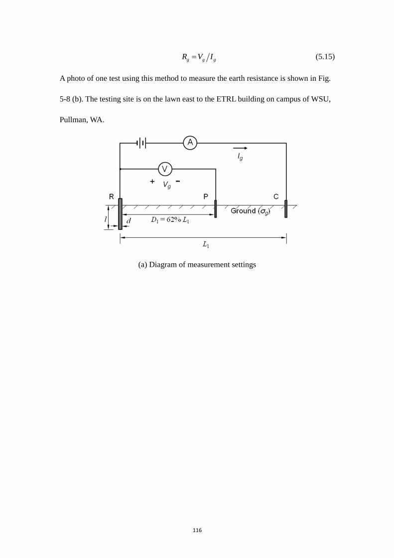
116

g g gR V I (5.15)

A photo of one test using this method to measure the earth resistance is shown in Fig.

5-8 (b). The testing site is on the lawn east to the ETRL building on campus of WSU,

Pullman, WA.

(a) Diagram of measurement settings

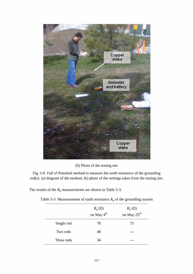
117

(b) Photo of the testing site

Fig. 5-8 Fall of Potential method to measure the earth resistance of the grounding

rod(s). (a) diagram of the method, (b) photo of the settings taken from the testing site.

The results of the Rg measurements are shown in Table 5-3.

Table 5-3 Measurements of earth resistance Rg of the grounding system

Rg (Ω)

on May 4th

Rg (Ω)

on May 25th

Single rod 78 75

Two rods 48 ---

Three rods 34 ---

118

To successfully conduct this experiment, the reflection coefficient ΓTL, defined in

(5.2), should be known in order to divide the current/voltage into forward and

backward waves. By using (5.2), (5.3) can be rewritten as

1

1

p f TL

f

p TL

si

V V

VI

Z

(5.16)

where Vp, Ip, and Vf are all phasors (complex numbers). It is necessary to know both

the magnitude and phase angle of Vp and Ip to uniquely determine ΓTL. However, in

practice, only the magnitudes of Vp and Ip are available. As a result, ΓTL cannot be

uniquely determined. Without adequate knowledge of ΓTL, it is difficult to get a

unique prediction of the behavior of the induced current in the sensor because the

value of ΓTL affects the incident fields on the sensor, and consequently induced current.

Thus, for preparing the experiments, it is important to have good estimates of ΓTL.

It is assumed that the load on the power line is nearly resistive because reactive

power is minimized. This means that the phase angle θTL of ΓTL should not be very

large. Taking the magnitude squared of both sides of the two equations in (5.16) and

dividing the first equation by the second one results in

2 22 21 1p TL p si TLV I Z

After using cos sinTLj

TL TL TL TL TLr e r j and some simplifications, the above

equation can be rewritten as

21cos

2

TL

TL

TL

a b r

r a b

(5.17)

where a = |Vp|2 and b = |IpZsi|

2. Equation (5.17) shows the relation between the

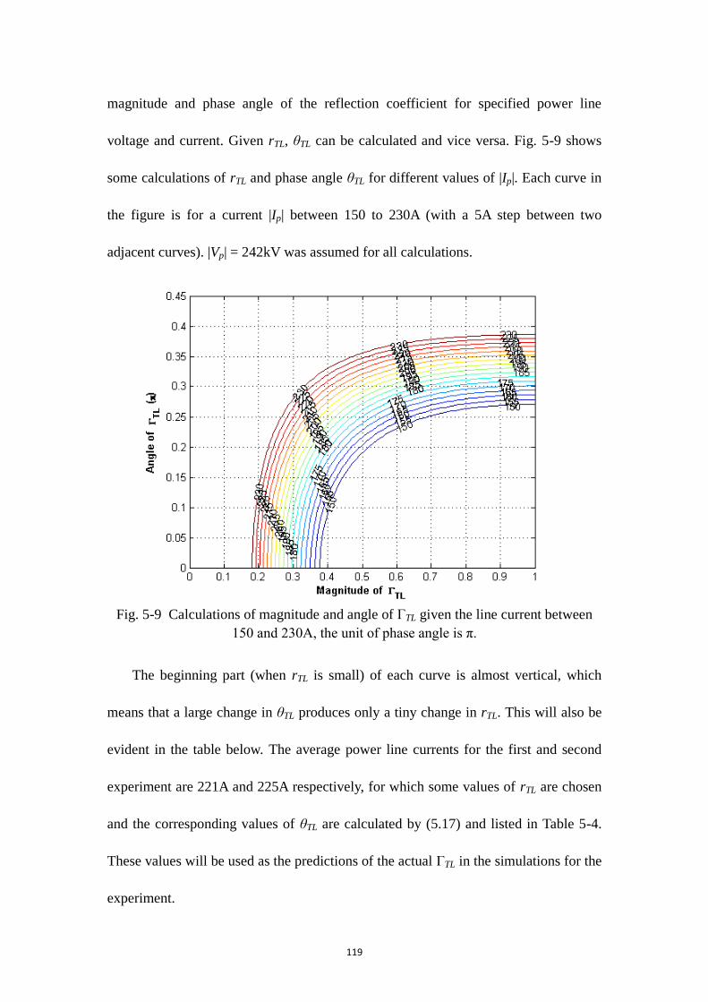
119

magnitude and phase angle of the reflection coefficient for specified power line

voltage and current. Given rTL, θTL can be calculated and vice versa. Fig. 5-9 shows

some calculations of rTL and phase angle θTL for different values of |Ip|. Each curve in

the figure is for a current |Ip| between 150 to 230A (with a 5A step between two

adjacent curves). |Vp| = 242kV was assumed for all calculations.

Fig. 5-9 Calculations of magnitude and angle of ΓTL given the line current between

150 and 230A, the unit of phase angle is π.

The beginning part (when rTL is small) of each curve is almost vertical, which

means that a large change in θTL produces only a tiny change in rTL. This will also be

evident in the table below. The average power line currents for the first and second

experiment are 221A and 225A respectively, for which some values of rTL are chosen

and the corresponding values of θTL are calculated by (5.17) and listed in Table 5-4.

These values will be used as the predictions of the actual ΓTL in the simulations for the

experiment.

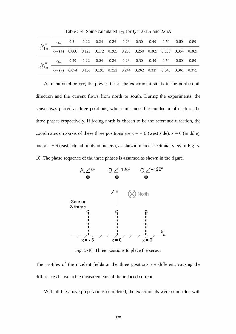
120

Table 5-4 Some calculated ΓTL for Ip = 221A and 225A

Ip =

221A

rTL 0.21 0.22 0.24 0.26 0.28 0.30 0.40 0.50 0.60 0.80

θTL (π) 0.080 0.121 0.172 0.205 0.230 0.250 0.309 0.338 0.354 0.369

Ip =

225A

rTL 0.20 0.22 0.24 0.26 0.28 0.30 0.40 0.50 0.60 0.80

θTL (π) 0.074 0.150 0.191 0.221 0.244 0.262 0.317 0.345 0.361 0.375

As mentioned before, the power line at the experiment site is in the north-south

direction and the current flows from north to south. During the experiments, the

sensor was placed at three positions, which are under the conductor of each of the

three phases respectively. If facing north is chosen to be the reference direction, the

coordinates on x-axis of these three positions are x = - 6 (west side), x = 0 (middle),

and x = + 6 (east side, all units in meters), as shown in cross sectional view in Fig. 5-

10. The phase sequence of the three phases is assumed as shown in the figure.

Fig. 5-10 Three positions to place the sensor

The profiles of the incident fields at the three positions are different, causing the

differences between the measurements of the induced current.

With all the above preparations completed, the experiments were conducted with

121

the procedures given below:

1) Run the simulation based on the parameters and predictions previously

obtained, calculate the value of Z1 or Z2 that could possibly cause the null in any of

the induced currents, and use this value as a reference.

2) Using only a identical resistance box at each end of the sensor, the values of

the two resistances were kept the same (Z1 = Z2 = R) and increased step by step.

Magnitudes of I1 and I2 are recorded for each step.

3) Add the capacitance box(es) in seires, adjust the values of the resistors and

capacitors to check whether there is an obvious null in I1 or I2. Take the measurement

of I1 and I2 and record the data.

4) Change the sensor‘s position (as shown in Fig. 5-10) and redo the processes

from 1) to 3).

5.2.3 Results and analysis

All the three positions of the sensor (see Fig. 5-10) were tried on May 4th

and only the

two positions under the side phase conductors (x = - 6 and x = + 6) were tested on

May 25th

. I1 is the induced current measured at the south end of the sensor and I2 is for

the north end. First, simulations are conducted for the experiments based on the

parameters previously determined. The values of Z1 (assumed Z2 = Z1) causing the

null in induced current and the resistances and capacitances that can realize these

values of Z1 in series or parallel connections are listed in Table 5-5, where Rs, Cs, Rp,

and Cp are the resistance and capacitance for the series and parallel connections,

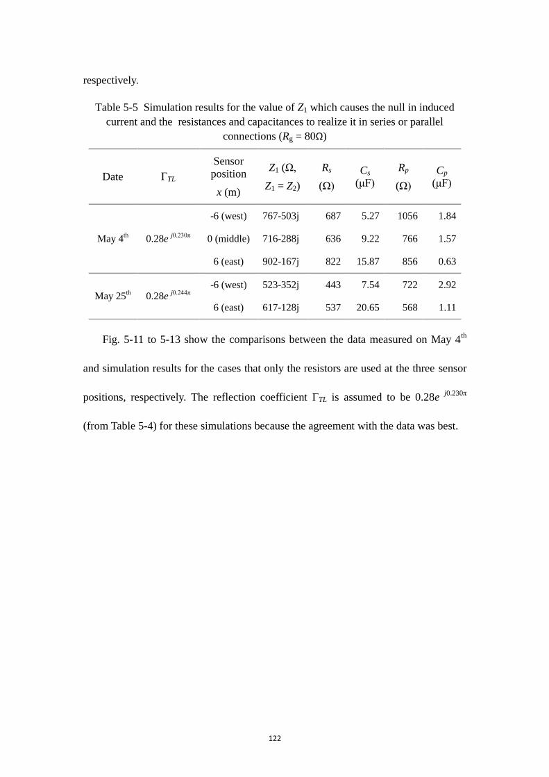
122

respectively.

Table 5-5 Simulation results for the value of Z1 which causes the null in induced

current and the resistances and capacitances to realize it in series or parallel

connections (Rg = 80Ω)

Date ΓTL

Sensor

position

x (m)

Z1 (Ω,

Z1 = Z2)

Rs

(Ω)

Cs

(μF)

Rp

(Ω)

Cp

(μF)

May 4th 0.28e

j0.230π

-6 (west) 767-503j 687 5.27 1056 1.84

0 (middle) 716-288j 636 9.22 766 1.57

6 (east) 902-167j 822 15.87 856 0.63

May 25th 0.28e

j0.244π

-6 (west) 523-352j 443 7.54 722 2.92

6 (east) 617-128j 537 20.65 568 1.11

Fig. 5-11 to 5-13 show the comparisons between the data measured on May 4th

and simulation results for the cases that only the resistors are used at the three sensor

positions, respectively. The reflection coefficient ΓTL is assumed to be 0.28e j0.230π

(from Table 5-4) for these simulations because the agreement with the data was best.

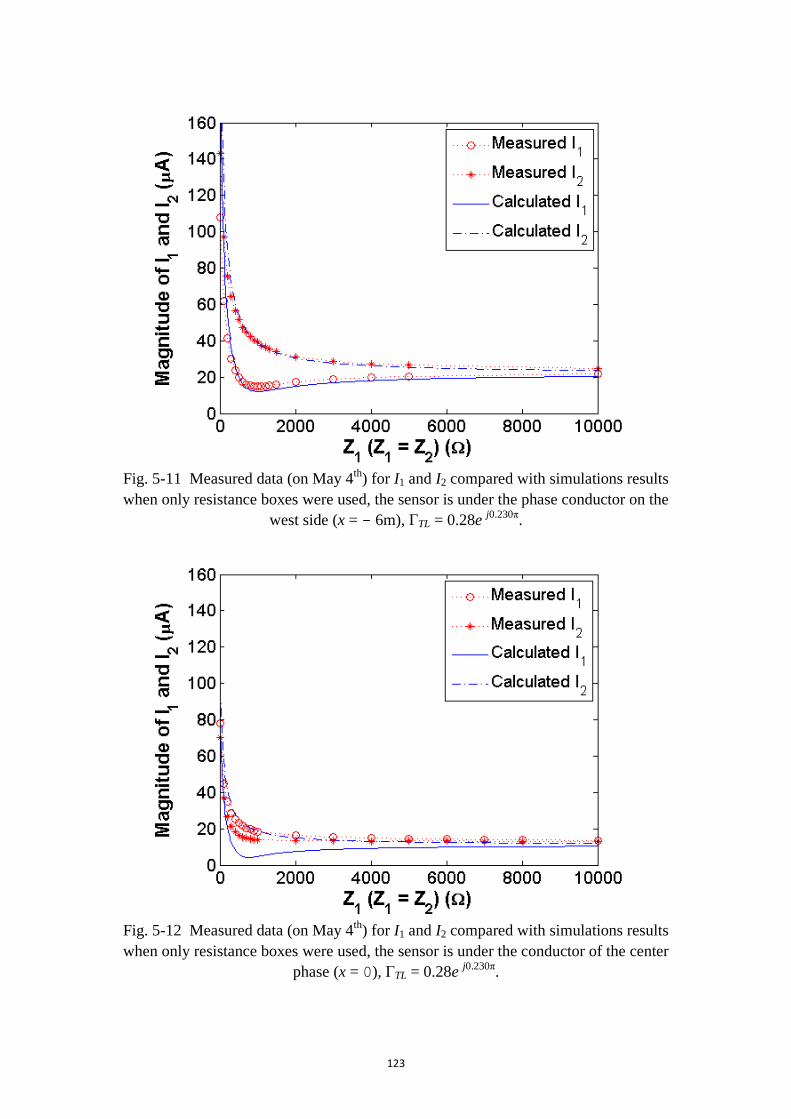
123

Fig. 5-11 Measured data (on May 4

th) for I1 and I2 compared with simulations results

when only resistance boxes were used, the sensor is under the phase conductor on the

west side (x = - 6m), ΓTL = 0.28e j0.230π

.

Fig. 5-12 Measured data (on May 4

th) for I1 and I2 compared with simulations results

when only resistance boxes were used, the sensor is under the conductor of the center

phase (x = 0), ΓTL = 0.28e j0.230π

.

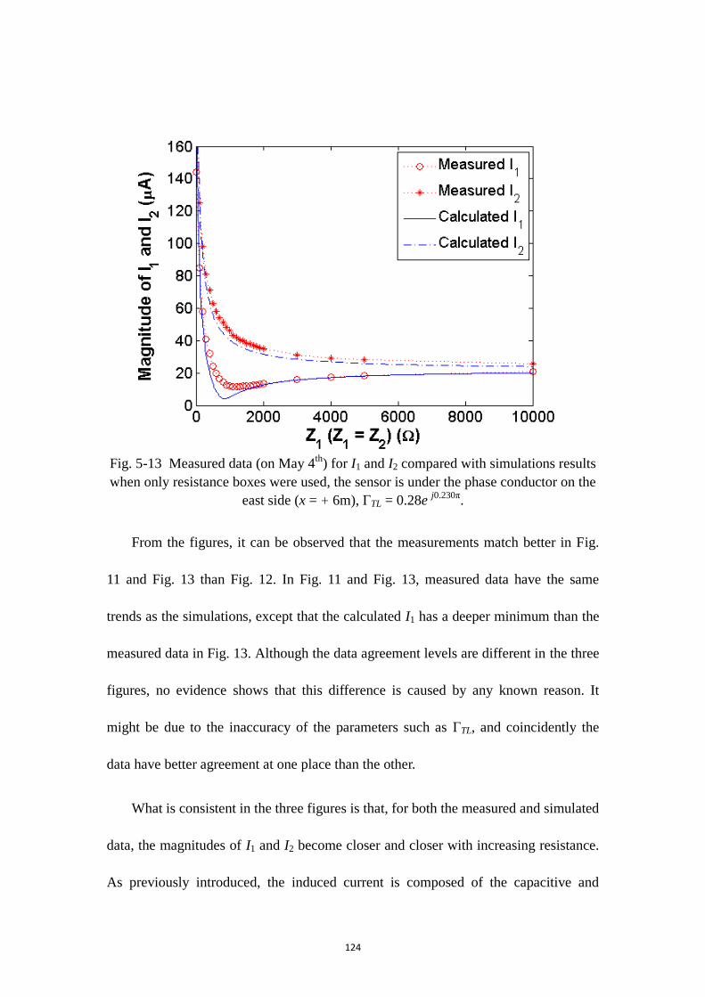
124

Fig. 5-13 Measured data (on May 4

th) for I1 and I2 compared with simulations results

when only resistance boxes were used, the sensor is under the phase conductor on the

east side (x = + 6m), ΓTL = 0.28e j0.230π

.

From the figures, it can be observed that the measurements match better in Fig.

11 and Fig. 13 than Fig. 12. In Fig. 11 and Fig. 13, measured data have the same

trends as the simulations, except that the calculated I1 has a deeper minimum than the

measured data in Fig. 13. Although the data agreement levels are different in the three

figures, no evidence shows that this difference is caused by any known reason. It

might be due to the inaccuracy of the parameters such as ΓTL, and coincidently the

data have better agreement at one place than the other.

What is consistent in the three figures is that, for both the measured and simulated

data, the magnitudes of I1 and I2 become closer and closer with increasing resistance.

As previously introduced, the induced current is composed of the capacitive and

125

inductive components. The capacitive component is due to the capacitive (high

impedance) coupling, independent of the resistance connected at the sensor‘s end, and

is symmetrical, about the midpoint of the sensor. On the other hand, the inductive

component is a loop current and dependent of the impedance in the circuit loop of the

sensor. Thus increasing of resistance suppresses the magnitude of the inductive

component and ultimately it can be ignored. Therefore, when the resistance is large

enough, what remains in the induced current is only the capacitive component and it

has same magnitude at the two ends of the sensor wire, i.e., I1 equals I2 then. The

measurements have proved this point in the three tests, providing the validation for

part (the capacitive coupling part) of the theory of the directional coupler.

Another useful result from the measurement is that one of I1 and I2 is always

larger than the other and it is consistent with the direction of the power line current,

which implies that, if the phase sequence is known, by comparing the magnitude of I1

and I2 the direction of the power line current can be determined.

The results of the experiment on May 25th

are similar to those for May 4th

except

that magnitude level of the induced currents is higher because the copper pipe (with

larger diameter and placed at higher position) was used as the sensor and this

enhances the capacitive coupling. Fig. 14 shows the results on May 25th

for the sensor

being under the phase conductor on the west side. The valley shape of I1 is more

obvious since the capacitive coupling was intentionally enhanced.

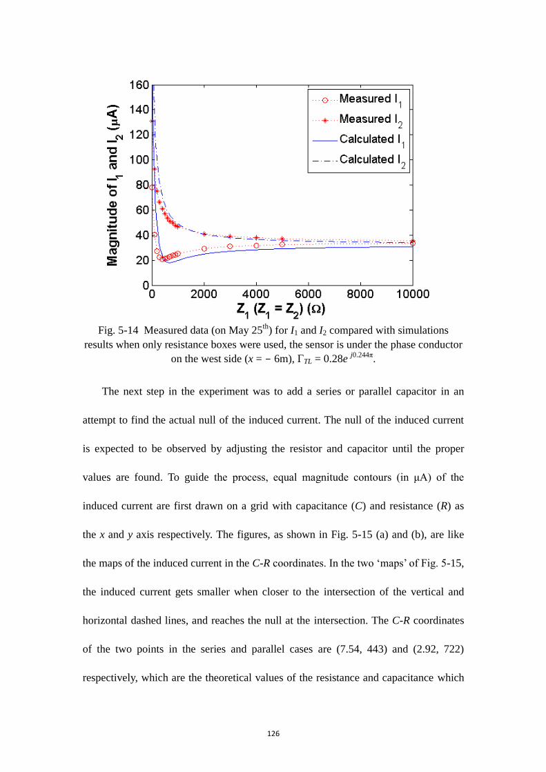
126

Fig. 5-14 Measured data (on May 25

th) for I1 and I2 compared with simulations

results when only resistance boxes were used, the sensor is under the phase conductor

on the west side (x = - 6m), ΓTL = 0.28e j0.244π

.

The next step in the experiment was to add a series or parallel capacitor in an

attempt to find the actual null of the induced current. The null of the induced current

is expected to be observed by adjusting the resistor and capacitor until the proper

values are found. To guide the process, equal magnitude contours (in μA) of the

induced current are first drawn on a grid with capacitance (C) and resistance (R) as

the x and y axis respectively. The figures, as shown in Fig. 5-15 (a) and (b), are like

the maps of the induced current in the C-R coordinates. In the two ‗maps‘ of Fig. 5-15,

the induced current gets smaller when closer to the intersection of the vertical and

horizontal dashed lines, and reaches the null at the intersection. The C-R coordinates

of the two points in the series and parallel cases are (7.54, 443) and (2.92, 722)

respectively, which are the theoretical values of the resistance and capacitance which

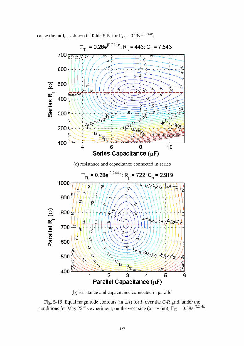
127

cause the null, as shown in Table 5-5, for ΓTL = 0.28e j0.244π

.

(a) resistance and capacitance connected in series

(b) resistance and capacitance connected in parallel

Fig. 5-15 Equal magnitude contours (in μA) for I1 over the C-R grid, under the

conditions for May 25th‘s experiment, on the west side (x = - 6m), ΓTL = 0.28e

j0.244π.

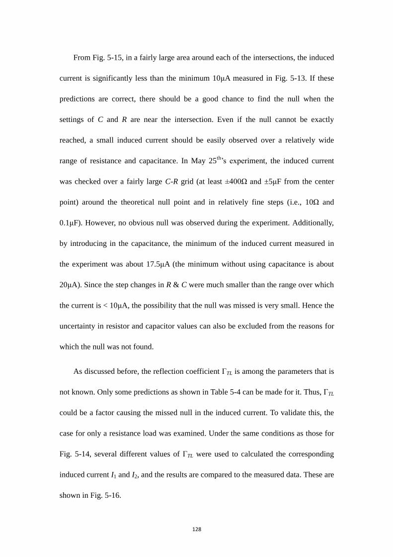
128

From Fig. 5-15, in a fairly large area around each of the intersections, the induced

current is significantly less than the minimum 10μA measured in Fig. 5-13. If these

predictions are correct, there should be a good chance to find the null when the

settings of C and R are near the intersection. Even if the null cannot be exactly

reached, a small induced current should be easily observed over a relatively wide

range of resistance and capacitance. In May 25th‘s experiment, the induced current

was checked over a fairly large C-R grid (at least ±400Ω and ±5μF from the center

point) around the theoretical null point and in relatively fine steps (i.e., 10Ω and

0.1μF). However, no obvious null was observed during the experiment. Additionally,

by introducing in the capacitance, the minimum of the induced current measured in

the experiment was about 17.5μA (the minimum without using capacitance is about

20μA). Since the step changes in R & C were much smaller than the range over which

the current is < 10μA, the possibility that the null was missed is very small. Hence the

uncertainty in resistor and capacitor values can also be excluded from the reasons for

which the null was not found.

As discussed before, the reflection coefficient ΓTL is among the parameters that is

not known. Only some predictions as shown in Table 5-4 can be made for it. Thus, ΓTL

could be a factor causing the missed null in the induced current. To validate this, the

case for only a resistance load was examined. Under the same conditions as those for

Fig. 5-14, several different values of ΓTL were used to calculated the corresponding

induced current I1 and I2, and the results are compared to the measured data. These are

shown in Fig. 5-16.

129

Fig. 5-16 Calculated I1 and I2 for different values of ΓTL and compared to the

measured data (on May 25th

) when only resistance boxes being used, the sensor is

under the phase conductor on the west side (x = - 6m).

Generally speaking, the results for ΓTL = 0.28e j0.244π

have the best agreement with

the measured data. This is why 0.28 was chosen to be the magnitude of ΓTL for all the

previous simulations. When the magnitude of ΓTL increases, the agreement becomes

worse, which validates the prediction made before that ΓTL should have relatively

small magnitude. Second, the capacitance is added in the simulations. Similar maps of

the induced current as shown in Fig. 5-15 are drawn for the cases that ΓTL = 0.5e j0.345π

and 0.8e j0.375π

(series connection of R and C) and shown in Fig. 5-17 (a) and (b),

respectively.

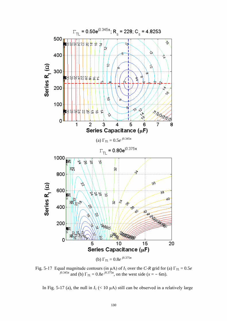
130

(a) ΓTL = 0.5e j0.345π

(b) ΓTL = 0.8e j0.375π

Fig. 5-17 Equal magnitude contours (in μA) of I1 over the C-R grid for (a) ΓTL = 0.5e j0.345π

and (b) ΓTL = 0.8e j0.375π

, on the west side (x = - 6m).

In Fig. 5-17 (a), the null in I1 (< 10 μA) still can be observed in a relatively large

131

area. Thus, similar comments made about Fig. 5-15 can apply here. However, in Fig.

5-17 (b), no null in I1 exists because the calculated Z1 for this case has negative real

part (the null would occur in the IV quadrant), which is physically impossible. So,

when the magnitude of ΓTL is large (0.8 for instance), it is possible that no null of the

induced current will occur for any values of the resistor and capacitor. From this point

of view, the reflection coefficient ΓTL could be the factor that causes no null to be

observed in the experiment. But based on the discussion made for Fig. 5-16, it is not

likely that ΓTL could have a large magnitude (close to 1). Therefore, the possibility

that ΓTL is the reason for the lack of a null is not strong.

Finally, it was noticed that the current on the power line is a little unbalanced (see

Table 5-1) with the three phase currents of 218, 237, and 225A, respectively.

Simulation results show that some unbalance situations for the power line current can

result in a value for Z1 that has a negative real part or positive imaginary part (which

means inductors instead of capacitors are required to find the null). For example,

assume the unbalanced three-phase currents are (218 18º, 237 -120º, 225 120º)

rather than the balanced ones (225 0º, 225 -120º, 225 120º), then the Z1 causing

the null is Z1 = 124 + j1107Ω, requiring inductor to be connected in the system. If that

is the case, the unbalance power line current could be the reason why the null is not

observed. But, again, the exact situation of the unbalance cannot be calculated due to

that the phase angle of the power line current is unknown. For this reason, it cannot be

concluded for certain that the unbalance of the power line current is the factor that

leads to the absence in a null being found.

132

Although the null has not been observed during the experiments and the reason

causing this is still not very clear, the results of the experiments provide strong (if not

perfect) validation for the theory of the directional coupler introduced in section 5.1.

The experiments are also helpful for understanding the mechanisms of the directional

coupler and revealing the problems related to using the directional coupler for power

transmission lines.

133

CHAPTER 6

LOW FREQUENCY DIPOLE IN THREE-LAYER MEDIUM

The subject of this chapter is independent of the research introduced in the first five

chapters. It is written in the dissertation because this project is an important part of my

research work during the time in Washington State University and some interesting

and useful results have been obtained from the study of the project.

The electromagnetic fields due to a dipole buried in the half-space or layered

conducting medium have been well studied for long time [57] – [61] This project is

composed by two parts. In the first part, the electromagnetic fields due to a dipole

(electric or magnetic, vertical or horizontal) placed above or buried in the upper layer

of a two-layer conducting medium are formulated by using the Sommerfeld integrals.

That is followed by the numerical validations for the formulations at the extremely

low frequency (ELF). In the second part, the ELF wave propagation in the conducting

medium when both the dipole and observation point are near the interface between the

free space and the conducting medium is studied by simplifying the formulations

obtained by the Sommerfeld integral method and interpreting the simplified results by

an up-over-and-down propagation model. To conveniently conduct this study, the two

layer conducting medium is replaced by a half space conducting medium since the

effect of the lower half space conducting medium on the fields can be ignored if the

thickness of the upper layer is large enough and the dipole and the observation point

are close enough to the upper interface. For this case, the source dipole is, again,

chosen to be a HED buried in the half space conducting medium.

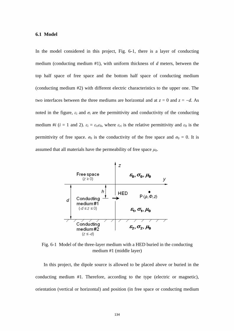
134

6.1 Model

In the model considered in this project, Fig. 6-1, there is a layer of conducting

medium (conducting medium #1), with uniform thickness of d meters, between the

top half space of free space and the bottom half space of conducting medium

(conducting medium #2) with different electric characteristics to the upper one. The

two interfaces between the three mediums are horizontal and at z = 0 and z = -d. As

noted in the figure, εi and ζi are the permittivity and conductivity of the conducting

medium #i (i = 1 and 2). εi = εriε0, where εri is the relative permittivity and ε0 is the

permittivity of free space. ζ0 is the conductivity of the free space and ζ0 = 0. It is

assumed that all materials have the permeability of free space μ0.

Fig. 6-1 Model of the three-layer medium with a HED buried in the conducting

medium #1 (middle layer)

In this project, the dipole source is allowed to be placed above or buried in the

conducting medium #1. Therefore, according to the type (electric or magnetic),

orientation (vertical or horizontal) and position (in free space or conducting medium

135

#1) of the dipole, there are eight different cases of dipole source to be studied, the

models of which are shown in Table 6-1.

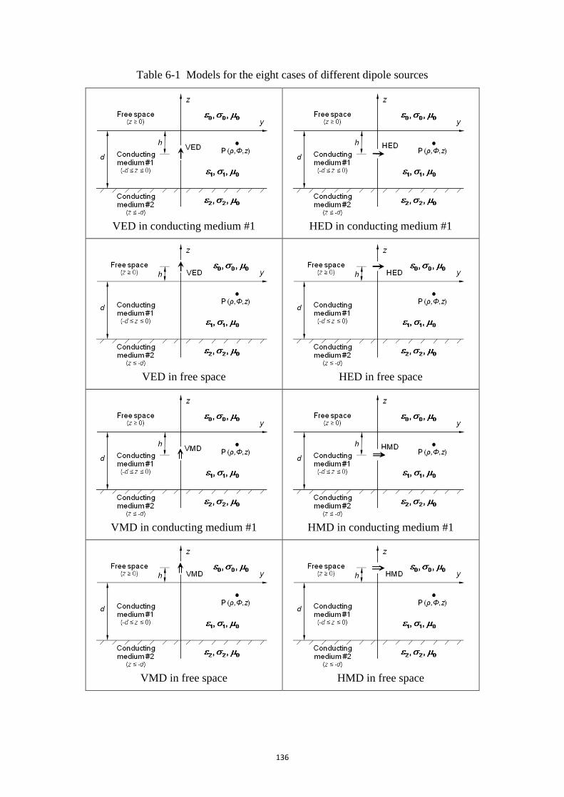
136

Table 6-1 Models for the eight cases of different dipole sources

VED in conducting medium #1

HED in conducting medium #1

VED in free space

HED in free space

VMD in conducting medium #1

HMD in conducting medium #1

VMD in free space

HMD in free space

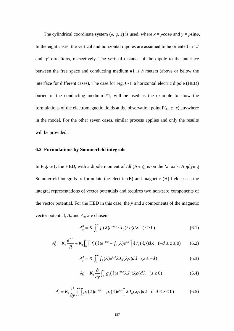
137

The cylindrical coordinate system (ρ, φ, z) is used, where x = ρcosφ and y = ρsinφ.

In the eight cases, the vertical and horizontal dipoles are assumed to be oriented in ‗z‘

and ‗y‘ directions, respectively. The vertical distance of the dipole to the interface

between the free space and conducting medium #1 is h meters (above or below the

interface for different cases). The case for Fig. 6-1, a horizontal electric dipole (HED)

buried in the conducting medium #1, will be used as the example to show the

formulations of the electromagnetic fields at the observation point P(ρ, φ, z) anywhere

in the model. For the other seven cases, similar process applies and only the results

will be provided.

6.2 Formulations by Sommerfeld integrals

In Fig. 6-1, the HED, with a dipole moment of Idl (A-m), is on the ‗z‘ axis. Applying

Sommerfeld integrals to formulate the electric (E) and magnetic (H) fields uses the

integral representations of vector potentials and requires two non-zero components of

the vector potential. For the HED in this case, the y and z components of the magnetic

vector potential, Ay and Az, are chosen.

00

1 1 00

( ) ( ) ( 0)u z

yA K f e J d z

(6.1)

1

1 11

1 1 2 3 00

( ) ( ) ( ) ( 0)R

u z u z

y

eA K K f e f e J d d z

R

(6.2)

22

1 4 00

( ) ( ) ( )u z

yA K f e J d z d

(6.3)

00

1 1 00

( ) ( ) ( 0)u z

zA K g e J d zy

(6.4)

1 11

1 2 3 00

( ) ( ) ( ) ( 0)u z u z

zA K g e g e J d d zy

(6.5)

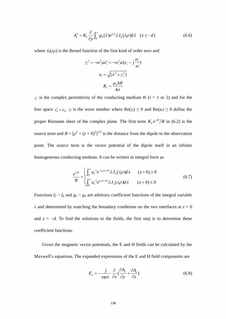
138

22

1 4 00

( ) ( ) ( )u z

zA K g e J d z dy

(6.6)

where J0(λρ) is the Bessel function of the first kind of order zero and

2 2 2 ( )ii i i j

2 2( )i iu

01

4

IdlK

i is the complex permittivity of the conducting medium #i (i = 1 or 2) and for the

free space 0 0 . γi is the wave number where Re(γi) ≤ 0 and Re(ui) ≥ 0 define the

proper Riemann sheet of the complex plane. The first term 1

1

RK e R in (6.2) is the

source term and R = [ρ2 + (z + h)

2]

1/2 is the distance from the dipole to the observation

point. The source term is the vector potential of the dipole itself in an infinite

homogeneous conducting medium. It can be written in integral form as

11

1

( )1

1 00

( )1

1 00

( ) ( ) 0

( ) ( ) 0

u z hR

u z h

u e J d z he

R u e J d z h

(6.7)

Functions f1 ~ f4 and g1 ~ g4 are arbitrary coefficient functions of the integral variable

λ and determined by matching the boundary conditions on the two interfaces at z = 0

and z = -d. To find the solutions to the fields, the first step is to determine these

coefficient functions.

Given the magnetic vector potentials, the E and H fields can be calculated by the

Maxwell‘s equations. The expanded expressions of the E and H field components are

( )y z

x

A AjE

x y z

(6.8)

139

2( )y z

y y

A AjE A

y y z

(6.9)

2( )y z

z z

A AjE A

z y z

(6.10)

1( )

yzx

AAH

y z

(6.11)

1 zy

AH

x

(6.12)

1 y

z

AH

x

(6.13)

The boundary conditions to be satisfied are that all the tangential fields are continuous

on the interfaces at z = 0 and z = -d plane. They can be written as

On z = 0 plane On z = -d plane

0 10 1

0 1

1 1y yz zA AA A

y z y z

2 12 1

2 1

1 1y yz zA AA A

y z y z

0 1

y yA A 2 1

y yA A

0 1

z zA A 2 1

z zA A

0 1

y yA A

z z

2 1

y yA A

z z

Inserting the vector potentials from (6.1) through (6.6) into these boundary conditions

and solving for the coefficient functions result in

1 1( ) ( )

1 2 1 2 1

2 u h d u h df u u e u u eD

(6.14)

1 12 1 ( ) ( )

2 1 0 0 1

1

u h d u h du uf u u e u u e

u D

(6.15)

1 10 1 ( ) ( )

3 1 2 2 1

1

u h d u h du uf u u e u u e

u D

(6.16)

2

1 1

4 0 1 0 1

2u d

u h u hef u u e u u e

D

(6.17)

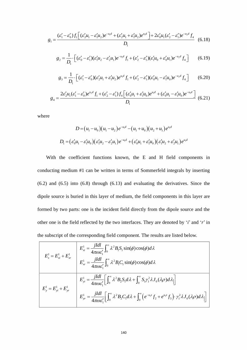
140

1 1 2

1 0 1 2 1 1 2 2 1 1 2 0 1 2 1 4

1

1

( ) ( ) ( ) 2 ( )u d u d u df u u e u u e u e f

gD

(6.18)

1 2

2 0 1 1 2 2 1 1 2 1 1 0 0 1 4

1

1( )( ) ( )( )

u d u dg u u e f u u e f

D (6.19)

1 2

3 1 0 2 1 1 2 1 2 1 0 1 1 0 4

1

1( )( ) ( )( )

u d u dg u u e f u u e f

D (6.20)

2 1 1

2 1 1 0 1 2 1 4 0 1 1 0 0 1 1 0

4

1

2 ( ) ( ) ( ) ( )u d u d u du e f f u u e u u e

gD

(6.21)

where

1 1

1 0 1 2 1 0 2 1

u d u dD u u u u e u u u u e

1 1

1 0 1 1 0 1 2 2 1 0 1 1 0 1 2 2 1

u d u dD u u u u e u u u u e

With the coefficient functions known, the E and H field components in

conducting medium #1 can be written in terms of Sommerfeld integrals by inserting

(6.2) and (6.5) into (6.8) through (6.13) and evaluating the derivatives. Since the

dipole source is buried in this layer of medium, the field components in this layer are

formed by two parts: one is the incident field directly from the dipole source and the

other one is the field reflected by the two interfaces. They are denoted by ‗i‘ and ‗r‘ in

the subscript of the corresponding field component. The results are listed below.

1 1 1

x xi xrE E E

1 2

1 10

1

sin( )cos( )4

xi

jIdlE B S d

1 2

1 10

1

sin( )cos( )4

xr

jIdlE B C d

1 1 1

y yi yrE E E

1 2 2

2 1 1 1 00 0

1

( )4

yi

jIdlE B S d S J d

1 11 2 2

2 1 2 3 1 00 0

1

( )4

u z u z

yr

jIdlE B C d e f e f J d

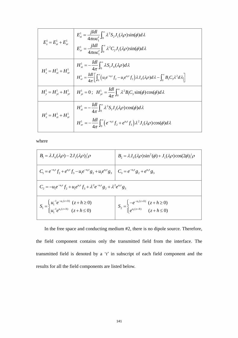
141

1 1 1

z zi zrE E E

1 2

2 10

1

( )sin( )4

zi

jIdlE S J d

1 2

2 10

1

( )sin( )4

zr

jIdlE C J d

1 1 1

x xi xrH H H

1

1 00

( )4

xi

IdlH S J d

1 11 2

1 2 1 3 0 2 30 0

( )4

u z u z

xr

IdlH u e f u e f J d B C d

1 1 1

y yi yrH H H 1 0yiH ; 1 2

1 30

sin( )cos( )4

yr

IdlH B C d

1 1 1

z zi zrH H H

1 2

1 10

( )cos( )4

zi

IdlH S J d

1 11 2

2 3 10

( )cos( )4

u z u z

zr

IdlH e f e f J d

where

1 0 1( ) 2 ( )B J J 2

2 0 1( )sin ( ) ( )cos(2 )B J J

1 1 1 1

1 2 3 1 2 1 3

u z u z u z u zC e f e f u e g u e g 1 1

3 2 3

u z u zC e g e g

1 1 1 12 2

2 1 2 1 3 2 3

u z u z u z u zC u e f u e f e g e g

1

1

( )1

1

1 ( )1

1

( 0)

( 0)

u z h

u z h

u e z hS

u e z h

1

1

( )

2 ( )

( 0)

( 0)

u z h

u z h

e z hS

e z h

In the free space and conducting medium #2, there is no dipole source. Therefore,

the field component contains only the transmitted field from the interface. The

transmitted field is denoted by a ‗t‘ in subscript of each field component and the

results for all the field components are listed below.

142

E and H fields in the free space:

00 0 2

1 0 1 10

0

sin( )cos( )4

u z

x xt

jIdlE E f u g e B d

0 00 0 2 2

1 0 1 2 0 1 00 0

0

( )4

u z u z

y yt

jIdlE E f u g e B d e f J d

00 0 2 2

0 1 1 10

0

( )cos( )4

u z

z zt

jIdlE E u f g e J d

0 00 0 2

1 2 0 1 00 0

( )4

u z u z

x xt

IdlH H e g B d u e f J d

00 0 2

1 10

sin( )cos( )4

u z

y yt

IdlH H e g B d

00 0 2

1 10

( )cos( )4

u z

z zt

IdlH H e f J d

E and H fields in conducting medium #2:

22 2 2

4 2 4 10

2

sin( )cos( )4

u z

x xt

jIdlE E f u g e B d

2 22 2 2 2

4 2 4 2 2 4 00 0

2

( )4

u z u z

y yt

jIdlE E f u g e B d e f J d

22 2 2 2

2 4 4 10

2

( )cos( )4

u z

z zt

jIdlE E u f g e J d

2 22 2 2

4 2 2 4 00 0

( )4

u z u z

x xt

IdlH H e g B d u e f J d

22 2 2

4 10

sin( )cos( )4

u z

y yt

IdlH H e g B d

22 2 2

4 10

( )cos( )4

u z

z zt

IdlH H e f J d

The formulas of the E and H fields obtained in section 6.2 are evaluated by

numerical integrations conducted by programs written in Matlab. Under certain

143

conditions, the calculation results are compared to the quasi-static fields due to a HED

immersed in infinite medium for validation. The values of the parameters used in the

following simulations are listed in Table 6-2. The conductivity and permittivity of the

conducting medium #1 and #2 represent typical fresh lake water and lake bottom,

respectively.

Table 6-2 Parameters used in the simulations for the numerical validation

Medium Free space Conducting

medium #1

Conducting

medium #2

Relative permittivity, r 1 1 1

Conductivity, ζ (S/m) 0 0.018 0.012

Permeability, μ (H/m) 4π×10-7

4π×10-7

4π×10-7

d (m) 300

h (m) vary from 0 to 300

Dipole moment Idl (A-m) 1

Dipole frequency f (Hz) 10 to 3000

The method chosen for numerical integration is the composite Simpson‘s rule

[62], which is used to obtain the integration of a given integrand f(x) over interval [a,

b]. The integral formula of the Simpson‘s rule can be written as

5

(4)

1( ) ( ) 4 ( ) ( ) ( )3 90

b

a

h hf x dx f a f x f b f (6.22)

where x1 is the middle point of [a, b] and a ≤ ξ ≤ b. The Simpson‘s rule is usually

inaccurate if used over a large integration interval. To avoid this problem, a piecewise

approach, the composite Simpson‘s rule, is often applied (see Fig. 6-2).

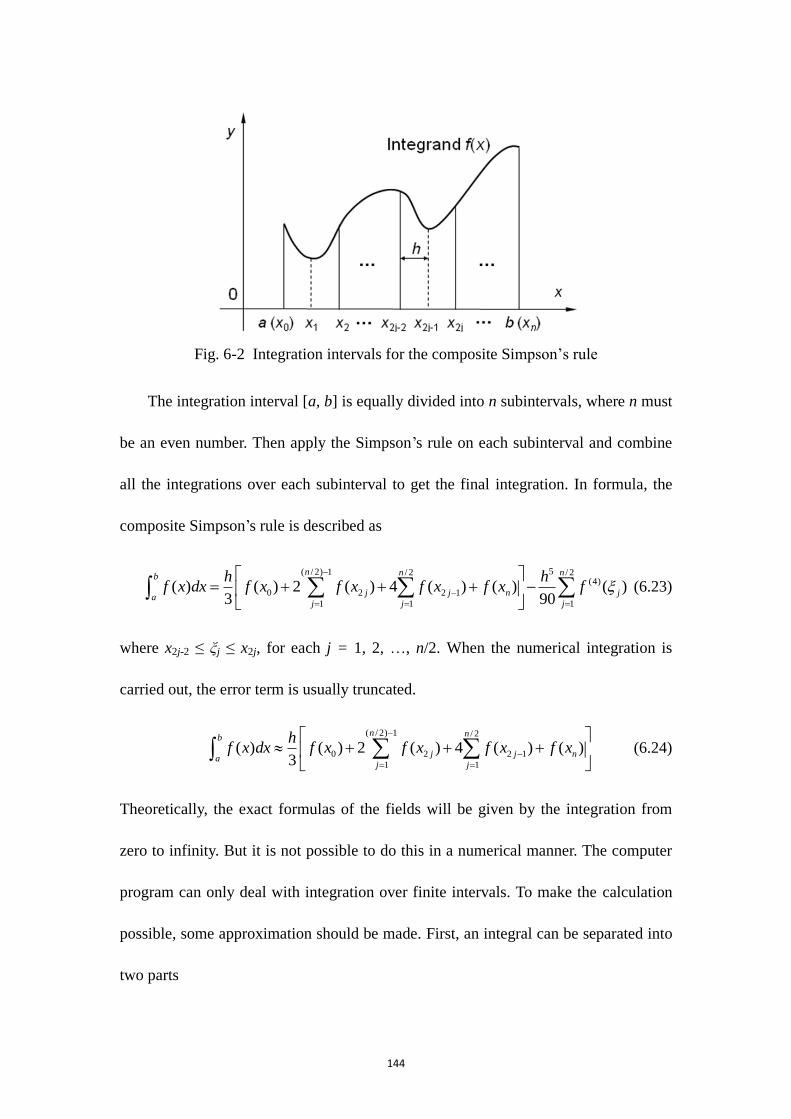
144

Fig. 6-2 Integration intervals for the composite Simpson‘s rule

The integration interval [a, b] is equally divided into n subintervals, where n must

be an even number. Then apply the Simpson‘s rule on each subinterval and combine

all the integrations over each subinterval to get the final integration. In formula, the

composite Simpson‘s rule is described as

5( / 2) 1 / 2 / 2(4)

0 2 2 1

1 1 1

( ) ( ) 2 ( ) 4 ( ) ( ) ( )3 90

n n nb

j j n ja

j j j

h hf x dx f x f x f x f x f

(6.23)

where x2j-2 ≤ ξj ≤ x2j, for each j = 1, 2, …, n/2. When the numerical integration is

carried out, the error term is usually truncated.

( / 2) 1 / 2

0 2 2 1

1 1

( ) ( ) 2 ( ) 4 ( ) ( )3

n nb

j j na

j j

hf x dx f x f x f x f x

(6.24)

Theoretically, the exact formulas of the fields will be given by the integration from

zero to infinity. But it is not possible to do this in a numerical manner. The computer

program can only deal with integration over finite intervals. To make the calculation

possible, some approximation should be made. First, an integral can be separated into

two parts

145

0 0( ) ( ) ( )

b

bf x dx f x dx f x dx

(6.25)

If a bound number ‗b‘ can be found such that the second integral on the right hand

side is small enough compared to the first integral, then the total integral can be

approximated by the first term. Since the integrands in the formulas of the fields have

attenuation characteristics, it is not difficult to find the bound number and the exact

integrals can be approximated by

max

0 0 max

max

0

( ) ( ) ( )

( )

FI d FI d FI d

FI d

(6.26)

where FI(λ) represents integrand for field integration, λmax is the upper limit of the

integration interval to be used in numerical calculation. In practice, for the parameters

given in Table 6-2, λmax is about 50 to 100 for the integrals due to the term

max1

1

max1

( )1

1 00

( )1

1 00

( ) ( ) 0

( ) ( ) 0

u z hR

u z h

u e J d z he

R u e J d z h

Usually, this value of λmax will give us enough accuracy for calculation. For the

reflected field integrals, which contain the coefficient functions f1 ~ f4 and g1 ~ g4, the

value of λmax is limited by the computation number limit of Matlab (about 10324

).

Usually, its range is from 1.0 to 2.5 for stable and acceptably accurate computation.

The integral step h is another important factor to the numerical integration. Too large

steps not only bring big error but also cause bad behavior (strong oscillation) of the

calculation. Small steps, however, slow down the speed of computation. The Bessel

functions are the major source of the oscillation. The integral step h is usually

determined by avoiding the oscillation of the Bessel functions and assuring the

146

computation speed at the same time. Typical value of h is chosen based on the rule

that the number of sample points on a wavelength of the Bessel function is between

30 to 50.

With the parameters of the integration being determined, the E and H fields due to

the HED shown in Fig. 6-1 are calculated by a Matlab program conducting the

composite Simpson‘s rule for the numerical integrations. The near-field results for the

case in which the HED is place at the middle of the conducting medium #1 are

compare to the quasi-static fields of the HED immersed in infinite conducting

medium #1. This is reasonable because the thickness of the conducting medium #1 is

large (300m) and the reflected fields due to the interfaces are very small and ignorable

if the HED is far away from the interfaces (such as at the middle of the layer).

Fig. 6-3 (a) and (b) show the results of Ex and Hz by the integration compared to the

corresponding quasi-static field components. The HED is 150 meters below the upper

interface (h = 150). The observation points are at z = -149m and on the axis having a

‗φ‘ angle of π/4. The frequency of the dipole is 1000Hz.

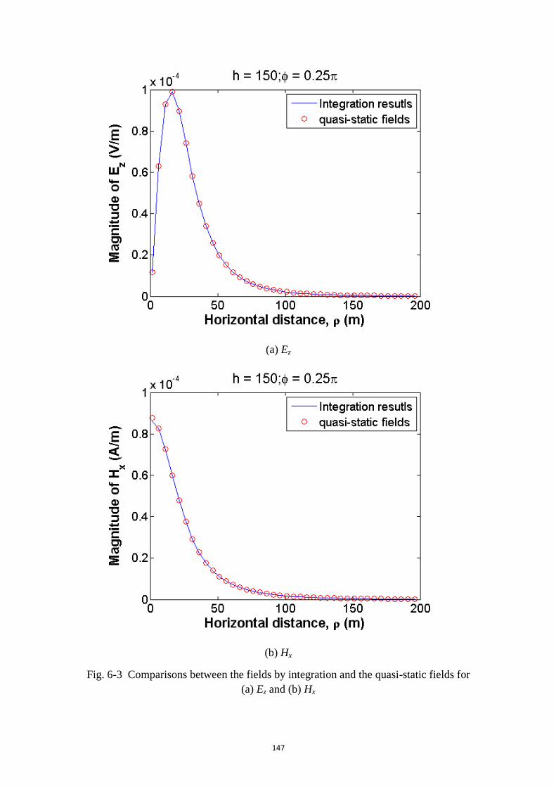
147

(a) Ez

(b) Hx

Fig. 6-3 Comparisons between the fields by integration and the quasi-static fields for

(a) Ez and (b) Hx

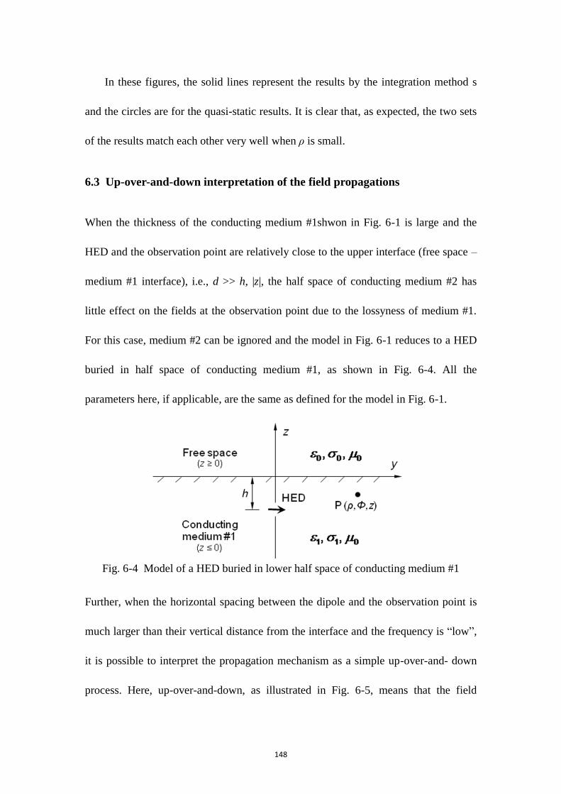
148

In these figures, the solid lines represent the results by the integration method s

and the circles are for the quasi-static results. It is clear that, as expected, the two sets

of the results match each other very well when ρ is small.

6.3 Up-over-and-down interpretation of the field propagations

When the thickness of the conducting medium #1shwon in Fig. 6-1 is large and the

HED and the observation point are relatively close to the upper interface (free space –

medium #1 interface), i.e., d >> h, |z|, the half space of conducting medium #2 has

little effect on the fields at the observation point due to the lossyness of medium #1.

For this case, medium #2 can be ignored and the model in Fig. 6-1 reduces to a HED

buried in half space of conducting medium #1, as shown in Fig. 6-4. All the

parameters here, if applicable, are the same as defined for the model in Fig. 6-1.

Fig. 6-4 Model of a HED buried in lower half space of conducting medium #1

Further, when the horizontal spacing between the dipole and the observation point is

much larger than their vertical distance from the interface and the frequency is ―low‖,

it is possible to interpret the propagation mechanism as a simple up-over-and- down

process. Here, up-over-and-down, as illustrated in Fig. 6-5, means that the field

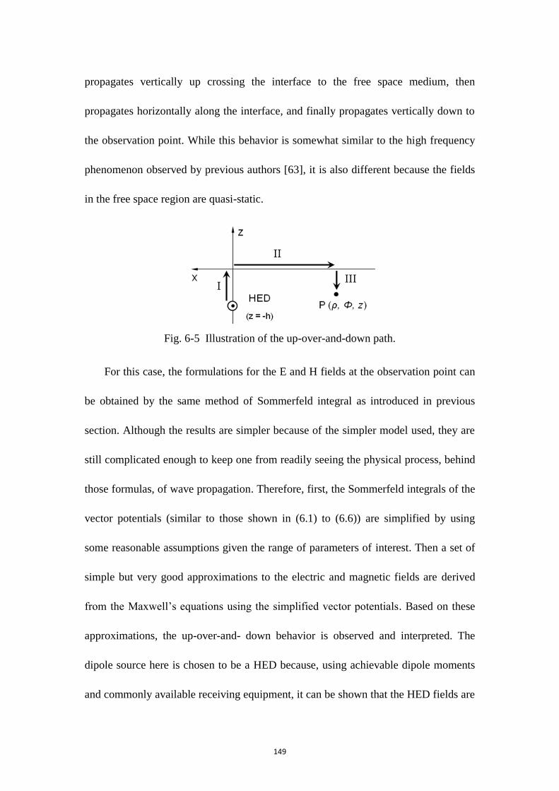
149

propagates vertically up crossing the interface to the free space medium, then

propagates horizontally along the interface, and finally propagates vertically down to

the observation point. While this behavior is somewhat similar to the high frequency

phenomenon observed by previous authors [63], it is also different because the fields

in the free space region are quasi-static.

Fig. 6-5 Illustration of the up-over-and-down path.

For this case, the formulations for the E and H fields at the observation point can

be obtained by the same method of Sommerfeld integral as introduced in previous

section. Although the results are simpler because of the simpler model used, they are

still complicated enough to keep one from readily seeing the physical process, behind

those formulas, of wave propagation. Therefore, first, the Sommerfeld integrals of the

vector potentials (similar to those shown in (6.1) to (6.6)) are simplified by using

some reasonable assumptions given the range of parameters of interest. Then a set of

simple but very good approximations to the electric and magnetic fields are derived

from the Maxwell‘s equations using the simplified vector potentials. Based on these

approximations, the up-over-and- down behavior is observed and interpreted. The

dipole source here is chosen to be a HED because, using achievable dipole moments

and commonly available receiving equipment, it can be shown that the HED fields are

150

detectable at larger distances than those of other dipole types (VED, VMD, and

HMD). To be more specified, it was assumed from this study that the maximum

dipole moments for electric and magnetic dipoles are 50 A-m and 2500 A-m2

respectively and that the minimum detectable electric and magnetic fields are 1μV/m

and 40μA/m respectively. Using these values, the horizontal electric field component

that is perpendicular to the HED direction can be detected to a distance of 800 meters

to the source. No other field component from any other dipole can be detected beyond

about 200 meters.

The vector potentials for using the Sommerfeld integral method are chosen to be

the y and z components of the magnetic vector potential, Ay and Az. They can be

written as

00

1 1 00

( ) ( ) ( 0)u z

yA K f e J d z

(6.27)

1 1

11

1 1 2 0 1 1 10

( ) ( ) ( 0)jk R jk R

u z

y y

e eA K K f e J d K K I z

R R

(6.28)

00

1 1 00

( ) ( ) ( 0)u z

zA K g e J d zy

(6.29)

11

1 2 0 1 10

( ) ( ) ( 0)u z

z zA K g e J d K I zy y

(6.30)

where J0(λρ) is the Bessel function of the first kind of order zero and

2 2 2

0 0 ( )ii i ik j

2 2( )i iu k

01

4

IdlK

εi’ is the complex permittivity of the ith

half space (i = 0 or 1 for free space and

151

conducting medium, respectively, and εi’ = ε0). ki is the wave number where Re(ki) ≥ 0

and Re(ui) ≥ 0 define the proper Reimann sheet of the complex plane. The first term

in (6.28) is the source term and R = [ρ2 + (z + h)

2]1/2

is the distance from the dipole to

the observation point. Iy1 and Iz1 represent the integral terms in (6.28) and (6.30),

respectively. The source term K1e-jk

1R/R in (6.28) is the vector potential of the dipole

itself in an infinite homogeneous conducting medium. It can be written in integral

form as

11

1

( )1

1 00

( )1

1 00

( ) ( ) 0

( ) ( ) 0

u z hjk R

u z h

u e J d z he

R u e J d z h

(6.31)

The coefficient functions f1, f2, g1 and g2 are determined by matching the boundary

conditions at z = 0.

1

1

0 1

2u he

fu u

(6.32)

1

1 0

2

1 0 1

u hu u ef

u u u

(6.33)

1

1 01 2

0 1 1 0 0 1

2( )

( )

u heg g

u u u u

(6.34)

6.3.1 Simplification of the integral of Iz1 and Iy1

The objective here is to derive simple but acceptable approximations for the fields,

which can be interpreted to provide good insight into the physical behavior of the

wave propagating from source to receiver. One fundamental problem with evaluating

the integrals shown in (6.27) to (6.30) is that, for large values of ρ compared to h and

z, the rapid oscillations of the Bessel function cause difficulties with the numerical

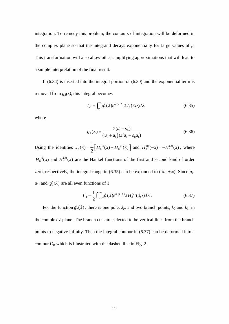
152

integration. To remedy this problem, the contours of integration will be deformed in

the complex plane so that the integrand decays exponentially for large values of ρ.

This transformation will also allow other simplifying approximations that will lead to

a simple interpretation of the final result.

If (6.34) is inserted into the integral portion of (6.30) and the exponential term is

removed from g2(λ), this integral becomes

1 ( )

1 2 00

( ) ( )u z h

zI g e J d

(6.35)

where

1 0

2

0 1 1 0 0 1

2( )( )

( )g

u u u u

(6.36)

Using the identities (1) (2)

0 0 0

1( ) ( ) ( )

2J x H x H x and (1) (2)

0 0( ) ( )H x H x , where

(1)

0 ( )H x and (2)

0 ( )H x are the Hankel functions of the first and second kind of order

zero, respectively, the integral range in (6.35) can be expanded to (-∞, +∞). Since u0,

u1, and 2 ( )g are all even functions of λ

1 ( ) (2)

1 2 0

1( ) ( )

2

u z h

zI g e H d

. (6.37)

For the function 2 ( )g , there is one pole, λp, and two branch points, k0 and k1, in

the complex λ plane. The branch cuts are selected to be vertical lines from the branch

points to negative infinity. Then the integral contour in (6.37) can be deformed into a

contour CB which is illustrated with the dashed line in Fig. 2.

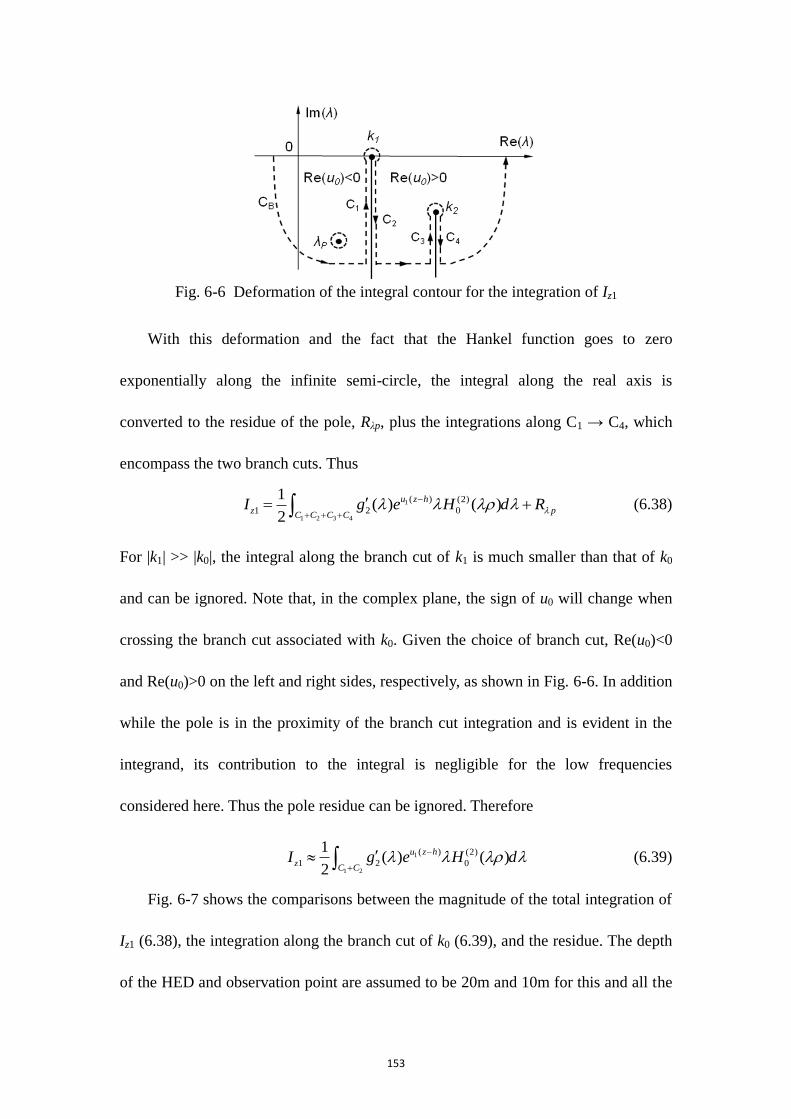
153

Fig. 6-6 Deformation of the integral contour for the integration of Iz1

With this deformation and the fact that the Hankel function goes to zero

exponentially along the infinite semi-circle, the integral along the real axis is

converted to the residue of the pole, Rλp, plus the integrations along C1 → C4, which

encompass the two branch cuts. Thus

1

1 2 3 4

( ) (2)

1 2 0

1( ) ( )

2

u z h

z pC C C C

I g e H d R

(6.38)

For |k1| >> |k0|, the integral along the branch cut of k1 is much smaller than that of k0

and can be ignored. Note that, in the complex plane, the sign of u0 will change when

crossing the branch cut associated with k0. Given the choice of branch cut, Re(u0)<0

and Re(u0)>0 on the left and right sides, respectively, as shown in Fig. 6-6. In addition

while the pole is in the proximity of the branch cut integration and is evident in the

integrand, its contribution to the integral is negligible for the low frequencies

considered here. Thus the pole residue can be ignored. Therefore

1

1 2

( ) (2)

1 2 0

1( ) ( )

2

u z h

zC C

I g e H d

(6.39)

Fig. 6-7 shows the comparisons between the magnitude of the total integration of

Iz1 (6.38), the integration along the branch cut of k0 (6.39), and the residue. The depth

of the HED and observation point are assumed to be 20m and 10m for this and all the

154

following simulations.

Fig. 6-7 Comparisons of magnitude between total integration, integration along

branch cut of k0, and the residue. (h = 20, z = -10)

Obviously, the integration along the branch cut of k1 and the residue are so small that

(6.39) has very good agreement with (6.38). Generally, (6.39) is valid when h, z << ρ,

|k1| >> |k0| and |k1ρ| >> 1.

Since ρ >> |h|, |z|, the decay of the integrand along C1 and C2 is controlled by the

value of |λρ|, the integral can be truncated at |λρ| = 10 and since we assume |λρ| >> 1

2 2 1/ 2

1 1 1( )u k jk (6.40)

With (6.40) the exponential term in (6.39) can be extracted from the integral, which

leads to

1

1 2

( )(2)

1 2 0( ) ( )2

jk z h

zC C

eI g H d

(6.41)

Further since |k0ρ| << 1 (i.e., quasi-static for z > 0), it is reasonable to assume that

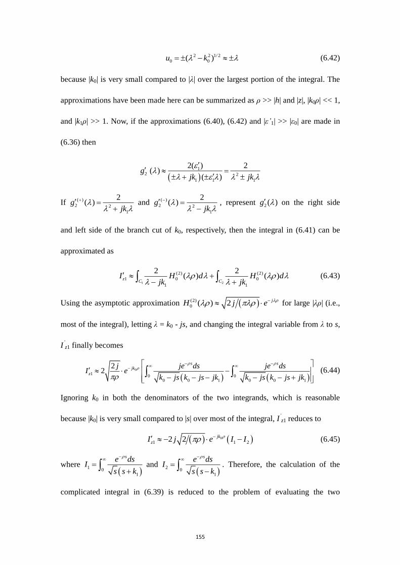
155

2 2 1/ 2

0 0( )u k (6.42)

because |k0| is very small compared to |λ| over the largest portion of the integral. The

approximations have been made here can be summarized as ρ >> |h| and |z|, |k0ρ| << 1,

and |k1ρ| >> 1. Now, if the approximations (6.40), (6.42) and |ε’1| >> |ε0| are made in

(6.36) then

1

2 2

1 1 1

2( ) 2( )

( )g

jk jk

If ( )

2 2

1

2( )g

jk

and ( )

2 2

1

2( )g

jk

, represent 2 ( )g on the right side

and left side of the branch cut of k0, respectively, then the integral in (6.41) can be

approximated as

1 2

(2) (2)

1 0 0

1 1

2 2( ) ( )z

C CI H d H d

jk jk

(6.43)

Using the asymptotic approximation (2)

0 ( ) 2 jH j e for large |λρ| (i.e.,

most of the integral), letting λ = k0 - js, and changing the integral variable from λ to s,

I’z1 finally becomes

0

10 0

0 0 1 0 0 1

22

s sjk

z

j je ds je dsI e

k js k js jk k js k js jk

(6.44)

Ignoring k0 in both the denominators of the two integrands, which is reasonable

because |k0| is very small compared to |s| over most of the integral, I’z1 reduces to

0

1 1 22 2jk

zI j e I I (6.45)

where

10

1

se dsI

s s k

and

20

1

se dsI

s s k

. Therefore, the calculation of the

complicated integral in (6.39) is reduced to the problem of evaluating the two

156

relatively simple integrals in (6.45). I1 can be analytically evaluated as [64]

1 1I k

Similarly for I2

2 1I k .

Therefore, the integral in (6.45) is

0

1

1

4 2jk

z

eI j

k

The integral Iz1 then can be approximated as

0

1 ( )

1

1

2 2jk

jk z h

z

eI je

k

(6.46)

It can be shown that (6.46) is approximately a factor of 1.4 larger than the exact

result in (6.35) and that this difference is relatively stable over a wide range of

parameters. Given this and the fact that an attempt to find a missing 2 factor did not

succeed, a further study of the approximation used to derive (6.46) was carried out.

This study indicated that the dominant part of the error resulted from the replacement

of the Hankel function by its asymptotic expansion. Given this, a correction term can

be written as

0 0(2)

00

1 1

1 1 22 ( )

Bjk jk s

CI e H j s e e dss k s k s

Clearly most of the contribution to this integral comes from small values of ρs. Thus

the integral is (somewhat arbitrarily) truncated at ρs = B = 0.3 and the Hankel function

is replaced by small argument expansion. Given this, the correction term is written as

0

01 1

1 1 2 1.7812 1 ln 2

2

Mjk

C

j j sI e s ds

s k s k

(6.47)

157

where inside the integral 0 1jk se e

and M = B/ρ. The integral in (6.47) can be

analytically evaluated and the result is

1 2 3C C C CI I I I (6.48)

where

011

1

lnjk

C

k BI c e

k B

0

2

1

8 jk

C

jBI e

k

0 1 1 1 1

3

1 1 1

2 222 ln ln

jk

C

k B j k B k B j k BI je j

k k B k B

2 1.7812 1 ln

2

j j Bc

.

IC1 and IC3 can be further simplified by expanding the natural logarithm function in

Taylor series.

0

1

1

2jk

C

MI c e

k

and 0

3

1

28

jk

C

jMI e

M k

The correction term is then rewritten as

0

1

jk

C

jNI e

k

(6.49)

where 2 8 8 2 ( )N M c M

is a constant. It is interesting to note that the

functional dependence of (6.49) is almost identical to that of (6.46). Hence adding

(6.49) to (6.46) results in

01 ( )

1

1

4 22

jkjk z h

z

e jeI N

k

(6.50)

which is identical to (6.46) except for the constant and that this constant is

approximately 1/1.4 times the constant in (6.46) when M = 0.3 (i.e., N ≈ 1.72). Then

158

(6.50) becomes

0

1 ( )

1

1

2jk

jk z h

z

eI je

k

(6.51)

When h, z << ρ, |k1| >> |k0| and |k1ρ| >> 1, (6.51) approximates the exact integral very

well. These conditions are roughly mapped to the following range of parameters: h, z

< 100m, 100Hz < f < 3000Hz, 500m < ρ < 10000m and 0.001S/m < ζ < 100S/m. The

error of (6.51) compared to the exact integral of Iz1 in (6.35) is less than 10% when

100Hz < f < 3000Hz and 500m < ρ < 10000m. Fig. 6-8 shows the comparisons of

magnitude and phase angle between the approximation in (6.51) and the exact integral

in (6.35), with dipole frequency of 1000Hz.

(a)

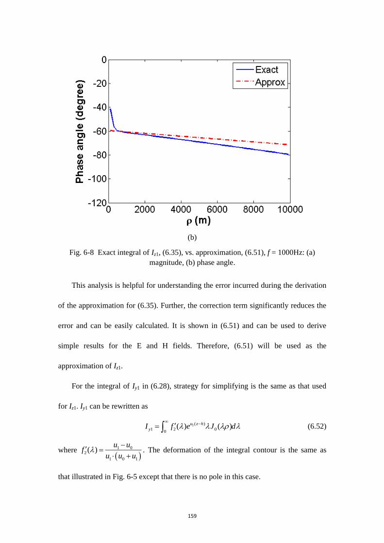
159

(b)

Fig. 6-8 Exact integral of Iz1, (6.35), vs. approximation, (6.51), f = 1000Hz: (a)

magnitude, (b) phase angle.

This analysis is helpful for understanding the error incurred during the derivation

of the approximation for (6.35). Further, the correction term significantly reduces the

error and can be easily calculated. It is shown in (6.51) and can be used to derive

simple results for the E and H fields. Therefore, (6.51) will be used as the

approximation of Iz1.

For the integral of Iy1 in (6.28), strategy for simplifying is the same as that used

for Iz1. Iy1 can be rewritten as

1 ( )

1 2 00

( ) ( )u z h

yI f e J d

(6.52)

where 1 0

2

1 0 1

( )u u

fu u u

. The deformation of the integral contour is the same as

that illustrated in Fig. 6-5 except that there is no pole in this case.

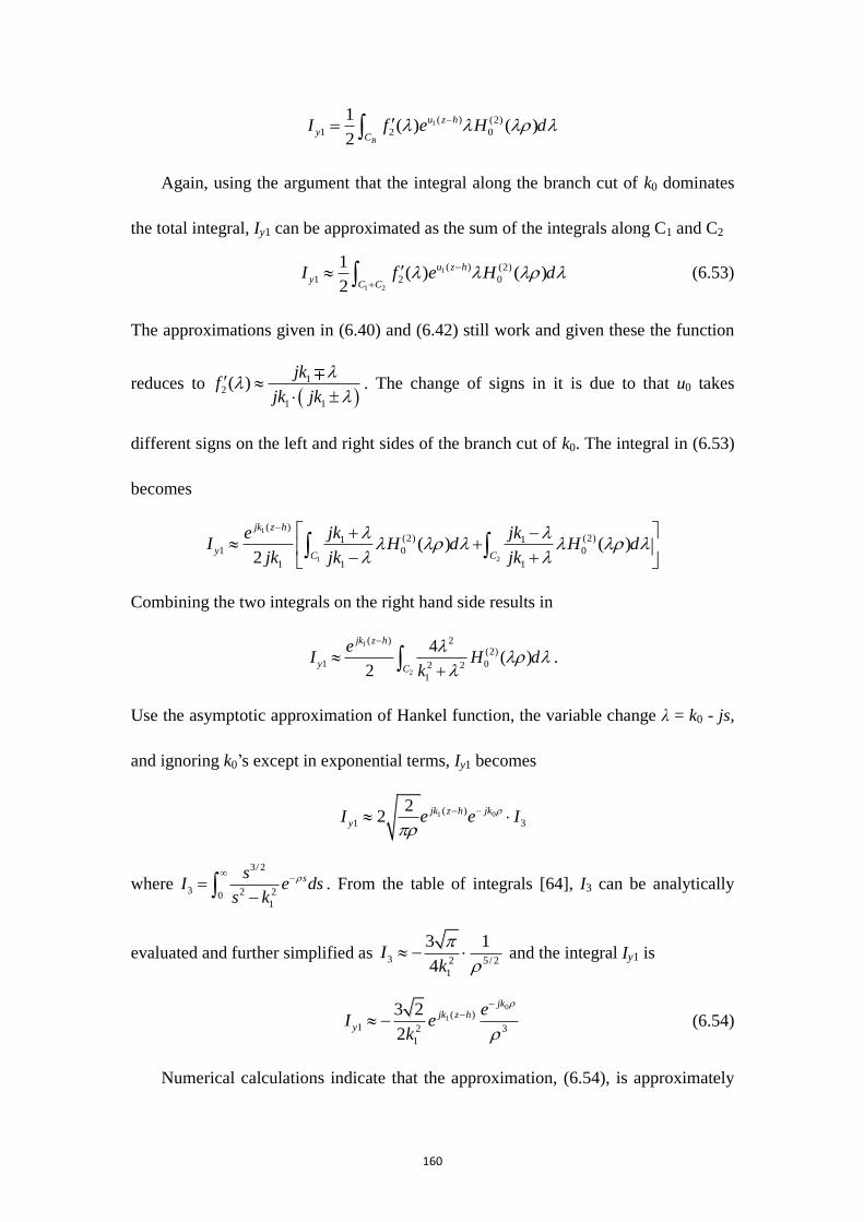
160

1 ( ) (2)

1 2 0

1( ) ( )

2 B

u z h

yC

I f e H d

Again, using the argument that the integral along the branch cut of k0 dominates

the total integral, Iy1 can be approximated as the sum of the integrals along C1 and C2

1

1 2

( ) (2)

1 2 0

1( ) ( )

2

u z h

yC C

I f e H d

(6.53)

The approximations given in (6.40) and (6.42) still work and given these the function

reduces to

12

1 1

( )jk

fjk jk

. The change of signs in it is due to that u0 takes

different signs on the left and right sides of the branch cut of k0. The integral in (6.53)

becomes

1

1 2

( )(2) (2)1 1

1 0 0

1 1 1

( ) ( )2

jk z h

yC C

jk jkeI H d H d

jk jk jk

Combining the two integrals on the right hand side results in

1

2

( ) 2(2)

1 02 2

1

4( )

2

jk z h

yC

eI H d

k

.

Use the asymptotic approximation of Hankel function, the variable change λ = k0 - js,

and ignoring k0‘s except in exponential terms, Iy1 becomes

01 ( )

1 3

22

jkjk z h

yI e e I

where 3/ 2

3 2 201

ssI e ds

s k

. From the table of integrals [64], I3 can be analytically

evaluated and further simplified as 3 2 5/ 2

1

3 1

4I

k

and the integral Iy1 is

0

1 ( )

1 2 3

1

3 2

2

jkjk z h

y

eI e

k

(6.54)

Numerical calculations indicate that the approximation, (6.54), is approximately

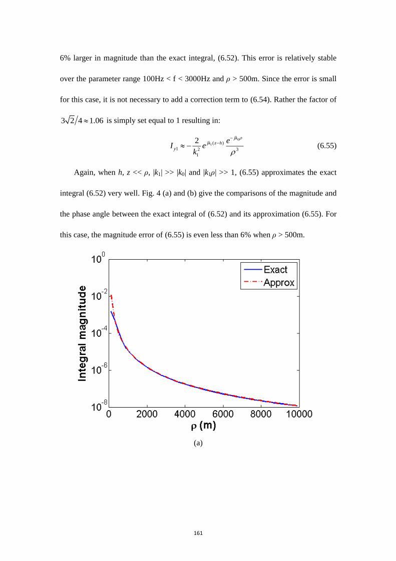
161

6% larger in magnitude than the exact integral, (6.52). This error is relatively stable

over the parameter range 100Hz < f < 3000Hz and ρ > 500m. Since the error is small

for this case, it is not necessary to add a correction term to (6.54). Rather the factor of

3 2 4 1.06 is simply set equal to 1 resulting in:

0

1 ( )

1 2 3

1

2jk

jk z h

y

eI e

k

(6.55)

Again, when h, z << ρ, |k1| >> |k0| and |k1ρ| >> 1, (6.55) approximates the exact

integral (6.52) very well. Fig. 4 (a) and (b) give the comparisons of the magnitude and

the phase angle between the exact integral of (6.52) and its approximation (6.55). For

this case, the magnitude error of (6.55) is even less than 6% when ρ > 500m.

(a)

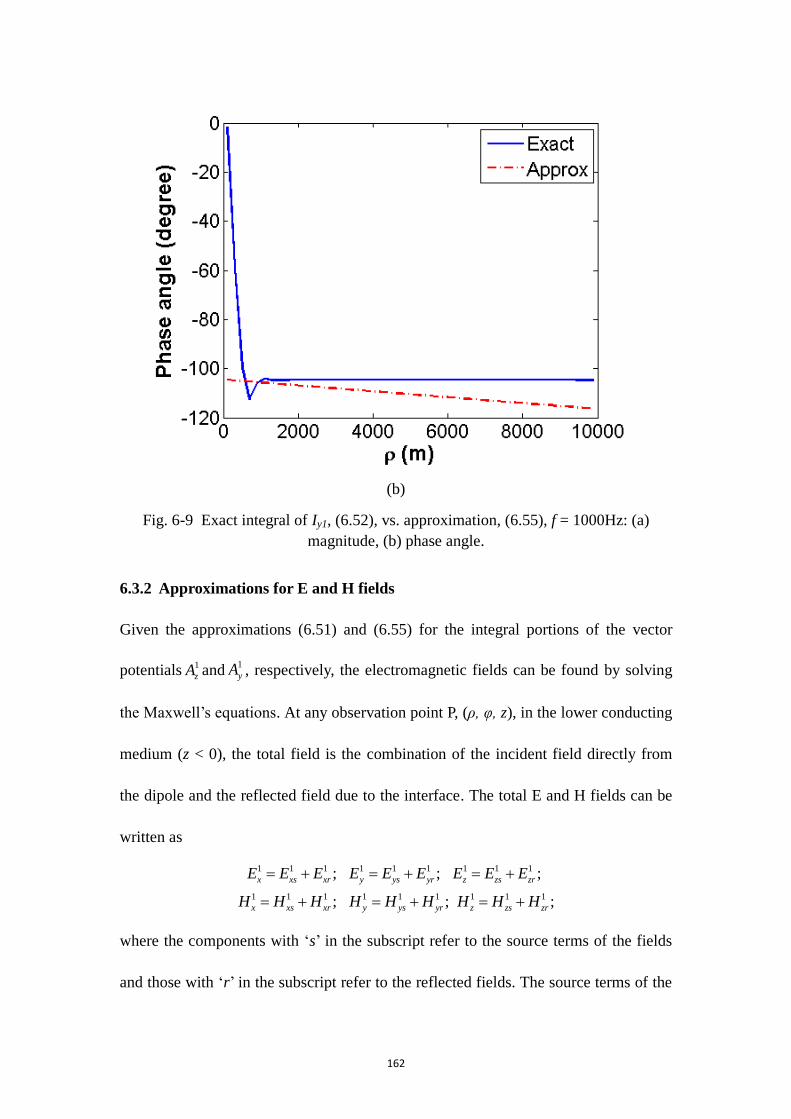
162

(b)

Fig. 6-9 Exact integral of Iy1, (6.52), vs. approximation, (6.55), f = 1000Hz: (a)

magnitude, (b) phase angle.

6.3.2 Approximations for E and H fields

Given the approximations (6.51) and (6.55) for the integral portions of the vector

potentials 1

zA and1

yA , respectively, the electromagnetic fields can be found by solving

the Maxwell‘s equations. At any observation point P, (ρ, φ, z), in the lower conducting

medium (z < 0), the total field is the combination of the incident field directly from

the dipole and the reflected field due to the interface. The total E and H fields can be

written as

1 1 1 1 1 1 1 1 1

1 1 1 1 1 1 1 1 1

; ; ;

; ; ;

x xs xr y ys yr z zs zr

x xs xr y ys yr z zs zr

E E E E E E E E E

H H H H H H H H H

where the components with ‗s‘ in the subscript refer to the source terms of the fields

and those with ‗r‘ in the subscript refer to the reflected fields. The source terms of the

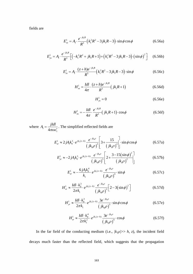
163

fields are

1

1 2 2

1 1 133 3 sin cos

jk R

xs

eE A k R jk R

R

(6.56a)

1

21 2 2 2 2

1 1 1 1 131 3 3 sin

jk R

ys

eE A k R jk R k R jk R

R

(6.56b)

1

1 2 2

1 1 15

( )3 3 sin

jk R

zs

z h eE A k R jk R

R

(6.56c)

1

1

13

( )1

4

jk R

xs

Idl z h eH jk R

R

(6.56d)

1 0ysH (6.56e)

1

1

131 cos

4

jk R

zs

Idl eH jk R

R

(6.56f)

where 1

14

jIdlA

. The simplified reflected fields are

0

1 ( )1 3

1 0 3 2

0 1

152 3 sin cos

jkjk z h

xr

eE jA k e

jk jk

(6.57a)

0

1

2

( )1 3

1 0 3 2

0 1

3 15 sin2 2

jkjk z h

yr

eE jA k e

jk jk

(6.57b)

0

1

4( )1 1 0

4

1 0

6sin

jkjk z h

zr

jA k eE e

k jk

(6.57c)

0

1

32( )1 0

3

1 0

2 3 sin2

jkjk z h

xr

Idl k eH e

k jk

(6.57d)

0

1

3( )1 0

3

1 0

3sin cos

2

jkjk z h

yr

Idl k eH e

k jk

(6.57e)

0

1

4( )1 0

42

1 0

3cos

2

jkjk z h

zr

Idl k eH e

k jk

(6.57f)

In the far field of the conducting medium (i.e., |k1ρ|>> h, z), the incident field

decays much faster than the reflected field, which suggests that the propagation

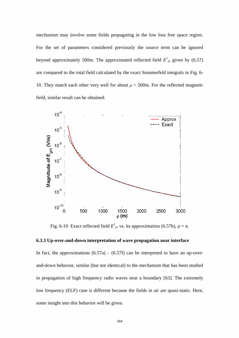
164

mechanism may involve some fields propagating in the low loss free space region.

For the set of parameters considered previously the source term can be ignored

beyond approximately 500m. The approximated reflected field E1

yr given by (6.57)

are compared to the total field calculated by the exact Sommerfeld integrals in Fig. 6-

10. They match each other very well for about ρ > 500m. For the reflected magnetic

field, similar result can be obtained.

Fig. 6-10 Exact reflected field E1yr vs. its approximation (6.57b), φ = π.

6.3.3 Up-over-and-down interpretation of wave propagation near interface

In fact, the approximations (6.57a) – (6.57f) can be interpreted to have an up-over-

and-down behavior, similar (but not identical) to the mechanism that has been studied

in propagation of high frequency radio waves near a boundary [63]. The extremely

low frequency (ELF) case is different because the fields in air are quasi-static. Here,

some insight into this behavior will be given.

165

At the observation point P (ρ, φ, z), consider the Ex component, which is

perpendicular to the HED‘s orientation and the easiest component to detect. As

discussed, the total field can be approximated by the corresponding reflected field

component in the far field (i.e., 6.57a). In the far field of the conducting medium the

second term in the bracket is small compared to the constant ‗3‘ and can be ignored.

Given this, the right hand side of (6.57a) can be rewritten as

01

11 1

3

1

3sin cos

2

jkjk hjk z

x

j Idl e eE e

k

(6.58)

where η1 is the intrinsic impedance of the conducting medium and η1 = (μ/ε’1)

1/2.

For the up-over-and-down process as illustrated in Fig. 6-5, the field generated by

the dipole (HED) first propagates upward (Part I) and crosses the interface into the

free space region. Second, the wave spreads out horizontally (Part II) along the

interface. Note that since the upper medium is free space and for the whole range of ρ

considered here (i.e., 100 < ρ < 10,000m), |k0ρ|<<1, the fields in free space are quasi-

static. Finally, at the position on the interface right above P, the wave crosses the

interface again and propagates vertically down (Part III) to the observation point.

To identify (6.58) as an up-over-and-down process, it is important to show how

the different terms have functional dependencies that are characteristic to different

portions of the process. For example, it will be shown that in the ‗up‘ part of (6.58)

corresponds to propagation in medium #1 and the effect of crossing the interface can

be explained by image theory for dielectric-dielectric boundaries. To begin, it is

helpful to show how a quasi-static field in the air can be excited by the buried HED.

166

Since it is assumed that |k1h| << 1, the fields near the interface are quasi-static and can

be calculated using the electrostatic theory with charge dipole source as shown in

Fig.6-11 (a). The dipole moment is qdl (C-m) where q is related to the current, I, of

the original HED by

/dq

I j q q jIdt

(6.59)

Image theory for static charges near a dielectric-dielectric interface can be used to

find an expression for the electric field in the upper half space (air region). The lower

region is replaced by free space and the charges replaced by equivalent charges at the

same positions [65], as shown in Fig. 6-11 (b).

Fig. 6-11. (a) The static charge dipole replacing the HED and (b) the image of the

static dipole.

The equivalent charges are [65]

0

0 1

2Q q

(6.60)

and since ε0 << ε’1 (6.60) can be approximated by

0 12Q q (6.61)

The image charges form a new equivalent dipole with a moment Qdl, oriented in +y

direction that can be used to find the fields in the upper free space region. Using (6.59)

and (6.61) and known expressions for the fields of static dipoles, the electric field

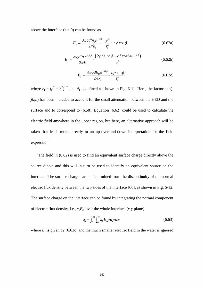
167

above the interface (z = 0) can be found as

1 2

1

5

1 1

3sin cos

2

jk h

x

qdl eE

k r

(6.62a)

12 2 2 2 2

1

5

1 1

2 sin cos

2

jk h

y

hqdl eE

k r

(6.62b)

1

1

5

1 1

3 sin

2

jk h

z

qdl e hE

k r

(6.62c)

where r1 = (ρ2 + h

2)1/2

and θ1 is defined as shown in Fig. 6-11. Here, the factor exp(-

jk1h) has been included to account for the small attenuation between the HED and the

surface and to correspond to (6.58). Equation (6.62) could be used to calculate the

electric field anywhere in the upper region, but here, an alternative approach will be

taken that leads more directly to an up-over-and-down interpretation for the field

expression.

The field in (6.62) is used to find an equivalent surface charge directly above the

source dipole and this will in turn be used to identify an equivalent source on the

interface. The surface charge can be determined from the discontinuity of the normal

electric flux density between the two sides of the interface [66], as shown in Fig. 6-12.

The surface charge on the interface can be found by integrating the normal component

of electric flux density, i.e., ε0Ez, over the whole interface (x-y plane)

2

00 0

s zq E d d

(6.63)

where Ez is given by (6.62c) and the much smaller electric field in the water is ignored.

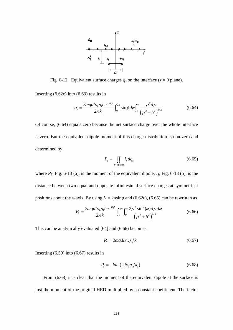
168

Fig. 6-12. Equivalent surface charges qs on the interface (z = 0 plane).

Inserting (6.62c) into (6.63) results in

1 22

0 1

5/ 20 0 2 21

3sin

2

jk h

s

qdl he dq d

k h

(6.64)

Of course, (6.64) equals zero because the net surface charge over the whole interface

is zero. But the equivalent dipole moment of this charge distribution is non-zero and

determined by

0plane

S S s

z

P l dq

(6.65)

where PS, Fig. 6-13 (a), is the moment of the equivalent dipole, lS, Fig. 6-13 (b), is the

distance between two equal and opposite infinitesimal surface charges at symmetrical

positions about the x-axis. By using lS = 2ρsinφ and (6.62c), (6.65) can be rewritten as

1 3 22

0 1

5/ 20 0 2 21

3 2 sin ( )

2

jk h

S

qdl he d dP

k h

(6.66)

This can be analytically evaluated [64] and (6.66) becomes

0 1 12SP qdl k (6.67)

Inserting (6.59) into (6.67) results in

0 1 1(2 )SP Idl j k (6.68)

From (6.68) it is clear that the moment of the equivalent dipole at the surface is

just the moment of the original HED multiplied by a constant coefficient. The factor

169

of 2 is due to imaging of the equivalent dipole in the ―nearly perfectly conducting‖

medium. Therefore, the ‗up‘ (Part I in Fig. 6-5) part of the propagation process can be

understood by noting that the fields from the original HED create an equivalent dipole

just above the interface.

Fig. 6-13 (a) Nonuniform distribution of the equivalent surface charge on the

interface (z = 0 plane); (b) geometry to find the moment of the dipole effect due to the

surface charge.

The fields in free space region can be calculated by assuming that the equivalent

dipole is in free space so that (on the z = 0 plane)

01

0

, 3

0

3( , ,0) sin cos

4

jkjk h

Sx u

P e eE

(6.69)

This is the ‗over‘ (Part II in Fig. 6) part of the propagation process. Finally, the field in

free space passes across the boundary with no attenuation due to the continuity of

tangential electric fields. Then, since the field is approximately constant on the

interface across a length much larger than the depth of P, the downward propagation

must be approximately 1jk ze (i.e., the ‗down‘ part of the propagation). Finally, the

expression of electric field component Ex at the observation point P is

01

11 1, 3

1

3( , , ) sin cos

2

jkjk hjk z

x u

j Idl e eE z e

k

(6.70)

170

which shows the complete up-over-and-down propagation. Equation (6.70) is

identical to (6.58).

For a summary, in this chapter, the formulations for the electric and magnetic

fields due to a low frequency HED buried in the middle layer of a three-layer medium

are derived based on the Sommerfeld integrals. The results are validated analytically

and numerically. Then, a method to simplify the Sommerfeld integrals for a HED

buried near an interface between free space and a conducting half space is introduced

(the lower two layers of the three-layer medium are reduced to half-space conducting

medium for convenience of analysis). Using this method, a simple approximation for

its electric fields in the conducting half space is obtained that is valid for distances

that are electrically small in free space and electrically large in the conducting

medium. The resulting approximation has been shown to be accurate within 10% over

a wide range of parameters for which h, z << ρ, |k1| >> |k0| and |k1ρ| >> 1. Finally, the

approximation can be interpreted as having up-over-and-down behavior for the

propagation path from the conducting medium to free space and vice versa.

171

REFERENCES

[1] Richard S. Nichols, ―The first electric power transmission line in North America-

Oregon City, Oregon,‖ IEEE Industry Applications Magazine, vol. 9, no. 4, pp. 7-

10, July, 2003.

[2] U.S. Department of Energy report, Five-Year Program Plan for Fiscal Years 2008

to 2012 for Electric Transmission and Distribution Programs, August, 2006.

[3] S. Chakrabarti, E. Kyriakides, T. Bi, D. Cai, and V. Terzija, ―Measurements get

together,‖ IEEE Power & Energy Magazine, vol. 7, no. 1, pp. 41-49, January,

2009.

[4] A. Phillips, ―Staying in shape,‖ IEEE Power & Energy Magazine, vol. 8, no. 2,

pp. 27-33, March, 2010.

[5] A. Phillips, ―Sensing the future,‖ IEEE Power & Energy Magazine, vol. 8, no. 6,

pp. 61-68, November, 2010.

[6] E. Fontana, S. C. Oliveira, et al., ―Novel system for leakage current detection on

insulator strings of overhead transmission lines,‖ IEEE Trans. on Power Del., vol.

21, no. 4, pp. 2064-2070, October, 2006.

[7] S. C. Oliveira, E. Fontana, and F. J. M. M. Cavalcanti, ―Leakage current activity

on glass-type insulators of overhead transmission lines in the northeast region of

Brazil,‖ IEEE Trans. on Power Del., vol. 24, no. 2, pp. 822-827, April, 2009.

[8] S. Han, R. Hao, and J. Lee, ―Inspection of insulators on high-voltage power

transmission lines,‖ IEEE Trans. on Power Del., vol. 24, no. 4, pp. 2319-2327,

October, 2009.

[9] X. Chen, C. Li, X. Huang, and et al., ―On-line estimating the level of

hydrophobicity of composite insulators using the digital images,‖ Proc. Electrical

Insulation Conf., pp. 216-221, 2005.

[10] J. Katrasnik, F. Pernus, and B. Likar, ―A survey of mobile robots for

distribution power line inspection,‖ IEEE Trans. on Power Del., vol. 25, no. 1, pp.

485-493, October, 2010.

[11] Y. Kobayashi, G. G. Karady, G. T. Heydt, and R. G. Olsen, ―The utilization of

satellite images to identify trees endangering transmission lines,‖ IEEE Trans. on

Power Del., vol. 24, no. 3, pp. 1703-1709, July, 2009.

[12] W. Villiers, J. H. Cloete, L. M. Wedepohl, and A. Burger, ―Real-time sag

monitoring system for high-voltage overhead transmission lines based on power-

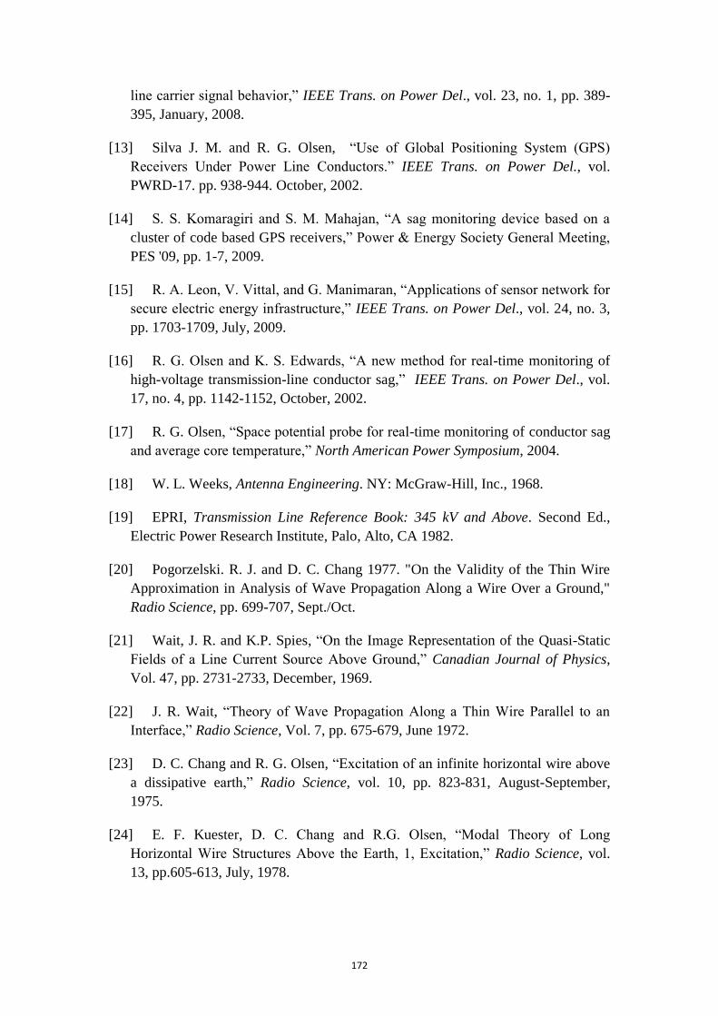
172

line carrier signal behavior,‖ IEEE Trans. on Power Del., vol. 23, no. 1, pp. 389-

395, January, 2008.

[13] Silva J. M. and R. G. Olsen, ―Use of Global Positioning System (GPS)

Receivers Under Power Line Conductors.‖ IEEE Trans. on Power Del., vol.

PWRD-17. pp. 938-944. October, 2002.

[14] S. S. Komaragiri and S. M. Mahajan, ―A sag monitoring device based on a

cluster of code based GPS receivers,‖ Power & Energy Society General Meeting,

PES '09, pp. 1-7, 2009.

[15] R. A. Leon, V. Vittal, and G. Manimaran, ―Applications of sensor network for

secure electric energy infrastructure,‖ IEEE Trans. on Power Del., vol. 24, no. 3,

pp. 1703-1709, July, 2009.

[16] R. G. Olsen and K. S. Edwards, ―A new method for real-time monitoring of

high-voltage transmission-line conductor sag,‖ IEEE Trans. on Power Del., vol.

17, no. 4, pp. 1142-1152, October, 2002.

[17] R. G. Olsen, ―Space potential probe for real-time monitoring of conductor sag

and average core temperature,‖ North American Power Symposium, 2004.

[18] W. L. Weeks, Antenna Engineering. NY: McGraw-Hill, Inc., 1968.

[19] EPRI, Transmission Line Reference Book: 345 kV and Above. Second Ed.,

Electric Power Research Institute, Palo, Alto, CA 1982.

[20] Pogorzelski. R. J. and D. C. Chang 1977. "On the Validity of the Thin Wire

Approximation in Analysis of Wave Propagation Along a Wire Over a Ground,"

Radio Science, pp. 699-707, Sept./Oct.

[21] Wait, J. R. and K.P. Spies, ―On the Image Representation of the Quasi-Static

Fields of a Line Current Source Above Ground,‖ Canadian Journal of Physics,

Vol. 47, pp. 2731-2733, December, 1969.

[22] J. R. Wait, ―Theory of Wave Propagation Along a Thin Wire Parallel to an

Interface,‖ Radio Science, Vol. 7, pp. 675-679, June 1972.

[23] D. C. Chang and R. G. Olsen, ―Excitation of an infinite horizontal wire above

a dissipative earth,‖ Radio Science, vol. 10, pp. 823-831, August-September,

1975.

[24] E. F. Kuester, D. C. Chang and R.G. Olsen, ―Modal Theory of Long

Horizontal Wire Structures Above the Earth, 1, Excitation,‖ Radio Science, vol.

13, pp.605-613, July, 1978.

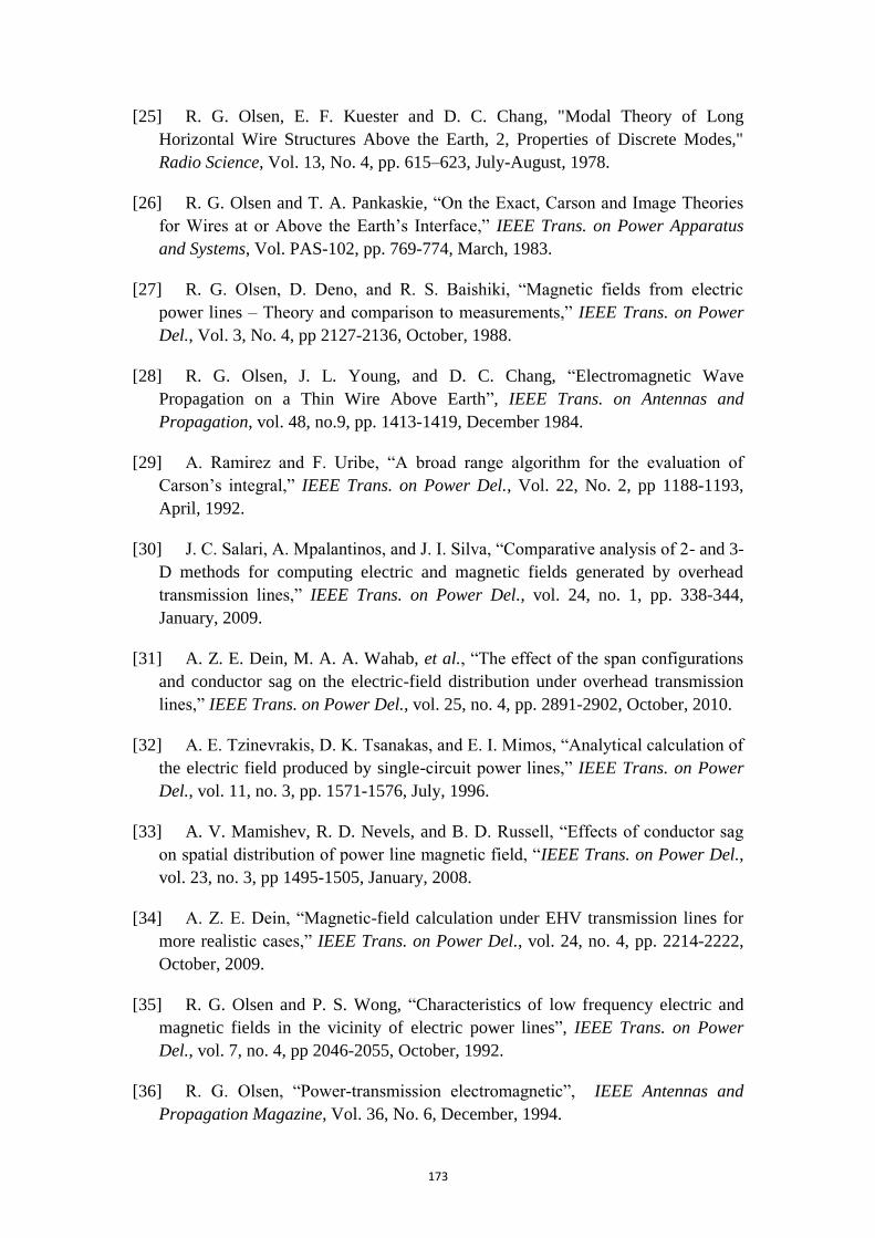
173

[25] R. G. Olsen, E. F. Kuester and D. C. Chang, "Modal Theory of Long

Horizontal Wire Structures Above the Earth, 2, Properties of Discrete Modes,"

Radio Science, Vol. 13, No. 4, pp. 615–623, July-August, 1978.

[26] R. G. Olsen and T. A. Pankaskie, ―On the Exact, Carson and Image Theories

for Wires at or Above the Earth‘s Interface,‖ IEEE Trans. on Power Apparatus

and Systems, Vol. PAS-102, pp. 769-774, March, 1983.

[27] R. G. Olsen, D. Deno, and R. S. Baishiki, ―Magnetic fields from electric

power lines – Theory and comparison to measurements,‖ IEEE Trans. on Power

Del., Vol. 3, No. 4, pp 2127-2136, October, 1988.

[28] R. G. Olsen, J. L. Young, and D. C. Chang, ―Electromagnetic Wave

Propagation on a Thin Wire Above Earth‖, IEEE Trans. on Antennas and

Propagation, vol. 48, no.9, pp. 1413-1419, December 1984.

[29] A. Ramirez and F. Uribe, ―A broad range algorithm for the evaluation of

Carson‘s integral,‖ IEEE Trans. on Power Del., Vol. 22, No. 2, pp 1188-1193,

April, 1992.

[30] J. C. Salari, A. Mpalantinos, and J. I. Silva, ―Comparative analysis of 2- and 3-

D methods for computing electric and magnetic fields generated by overhead

transmission lines,‖ IEEE Trans. on Power Del., vol. 24, no. 1, pp. 338-344,

January, 2009.

[31] A. Z. E. Dein, M. A. A. Wahab, et al., ―The effect of the span configurations

and conductor sag on the electric-field distribution under overhead transmission

lines,‖ IEEE Trans. on Power Del., vol. 25, no. 4, pp. 2891-2902, October, 2010.

[32] A. E. Tzinevrakis, D. K. Tsanakas, and E. I. Mimos, ―Analytical calculation of

the electric field produced by single-circuit power lines,‖ IEEE Trans. on Power

Del., vol. 11, no. 3, pp. 1571-1576, July, 1996.

[33] A. V. Mamishev, R. D. Nevels, and B. D. Russell, ―Effects of conductor sag

on spatial distribution of power line magnetic field, ―IEEE Trans. on Power Del.,

vol. 23, no. 3, pp 1495-1505, January, 2008.

[34] A. Z. E. Dein, ―Magnetic-field calculation under EHV transmission lines for

more realistic cases,‖ IEEE Trans. on Power Del., vol. 24, no. 4, pp. 2214-2222,

October, 2009.

[35] R. G. Olsen and P. S. Wong, ―Characteristics of low frequency electric and

magnetic fields in the vicinity of electric power lines‖, IEEE Trans. on Power

Del., vol. 7, no. 4, pp 2046-2055, October, 1992.

[36] R. G. Olsen, ―Power-transmission electromagnetic‖, IEEE Antennas and

Propagation Magazine, Vol. 36, No. 6, December, 1994.

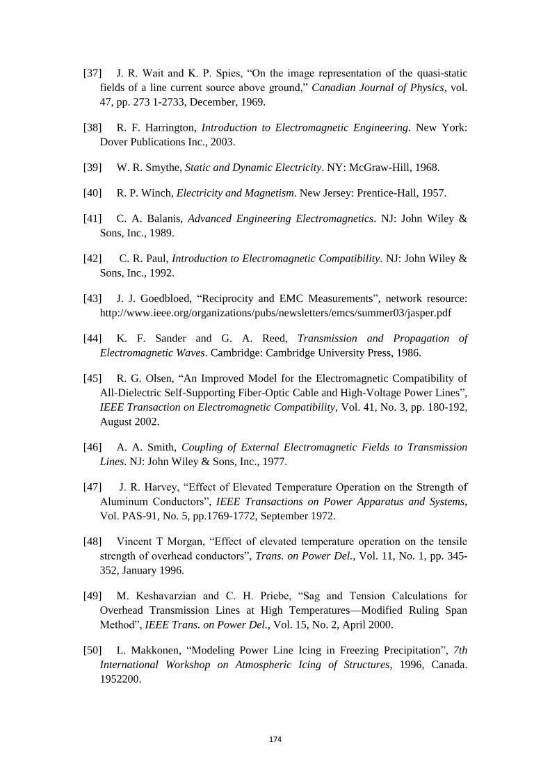
174

[37] J. R. Wait and K. P. Spies, ―On the image representation of the quasi-static

fields of a line current source above ground,‖ Canadian Journal of Physics, vol.

47, pp. 273 1-2733, December, 1969.

[38] R. F. Harrington, Introduction to Electromagnetic Engineering. New York:

Dover Publications Inc., 2003.

[39] W. R. Smythe, Static and Dynamic Electricity. NY: McGraw-Hill, 1968.

[40] R. P. Winch, Electricity and Magnetism. New Jersey: Prentice-Hall, 1957.

[41] C. A. Balanis, Advanced Engineering Electromagnetics. NJ: John Wiley &

Sons, Inc., 1989.

[42] C. R. Paul, Introduction to Electromagnetic Compatibility. NJ: John Wiley &

Sons, Inc., 1992.

[43] J. J. Goedbloed, ―Reciprocity and EMC Measurements‖, network resource:

http://www.ieee.org/organizations/pubs/newsletters/emcs/summer03/jasper.pdf

[44] K. F. Sander and G. A. Reed, Transmission and Propagation of

Electromagnetic Waves. Cambridge: Cambridge University Press, 1986.

[45] R. G. Olsen, ―An Improved Model for the Electromagnetic Compatibility of

All-Dielectric Self-Supporting Fiber-Optic Cable and High-Voltage Power Lines‖,

IEEE Transaction on Electromagnetic Compatibility, Vol. 41, No. 3, pp. 180-192,

August 2002.

[46] A. A. Smith, Coupling of External Electromagnetic Fields to Transmission

Lines. NJ: John Wiley & Sons, Inc., 1977.

[47] J. R. Harvey, ―Effect of Elevated Temperature Operation on the Strength of

Aluminum Conductors‖, IEEE Transactions on Power Apparatus and Systems,

Vol. PAS-91, No. 5, pp.1769-1772, September 1972.

[48] Vincent T Morgan, ―Effect of elevated temperature operation on the tensile

strength of overhead conductors‖, Trans. on Power Del., Vol. 11, No. 1, pp. 345-

352, January 1996.

[49] M. Keshavarzian and C. H. Priebe, ―Sag and Tension Calculations for

Overhead Transmission Lines at High Temperatures—Modified Ruling Span

Method‖, IEEE Trans. on Power Del., Vol. 15, No. 2, April 2000.

[50] L. Makkonen, ―Modeling Power Line Icing in Freezing Precipitation‖, 7th

International Workshop on Atmospheric Icing of Structures, 1996, Canada.

1952200.

175

[51] C. Meng and Y. Cheng, ―A New Ice Covering Model‖, 2008 International

Conference on High Voltage Engineering and Application, Chongqing, China,

November, 2008.

[52] M. W. Tuominen and R. G. Olsen, ―Electrical Design Parameters of All-

Dielectric-Self-Supporting Fiber Optic Cable‖, IEEE Transaction on Power

Delivery, Vol. 15, No. 3, pp. 940-947, July 2000.

[53] Internet resource, http://www.answers.com/topic/directional-coupler

[54] G. Metzger and J. Vabre, Transmission Lines With Pulse Excitation. NY:

Academic Press, 1969.

[55] Biddle Instruments, Getting Down to Earth: Manual on Earth-Resistance

Testing for the Practical Man, Fourth Edition, 1982.

[56] E. R. Sverko, ―Ground measuring techniques: electrode resistance to remote

earth & soil resistivity”, online resource:

[57] A. Baños, Dipole radiation in the presence of a conducting half-space. New

York: Pergamon, 1966.

[58] P. R. Bannister, ―Extension of finitely conducting earth-image-theory results

to any range‖, Naval Underwater Systems Center, New London, CT, Tech. Rep.,

Jan. 1984.

[59] J. R. Wait and L. L. Campbell, ―The fields of an oscillating magnetic dipole

immersed in a semi-infinite conducting medium‖, J. Geophys. Res., vol. 58, no. 2,

pp. 167-178, 1953.

[60] A. K. Sinha and P. K. Bhattacharya, ―Vertical magnetic dipole buried inside a

homogeneous earth‖, Radio Sci., vol. 1, no. 3, pp. 379-395, 1966.

[61] J. R. Wait, ―The electromagnetic fields of a horizontal dipole in the presence

of a conducting half-space‖, Can. J. Phys., vol. 39, no. 7, pp. 1017-1028, 1961.

[62] R. L. Burden and J. D. Faires, Numerical Analysis. MA: Brooks/Cole, 7th

edition, 2000.

[63] T. Tamir, ―Radio wave propagation along mixed paths in forest

environments‖, IEEE Trans. Antennas Propagat., vol. 25, no. 4, pp. 471-477, Jul.

1977.

[64] I. S. Gradshteyn and I. M. Ryzhik, Table of integrals series and products.

New York: Academic Press, 1965.

[65] E. D. Torre and C. V. Longo, The Electromagnetic Field. Boston: Allyn and

Bacon, Inc., 1969.