Algorithms in Java, 4th Edition · Robert Sedgewick and Kevin Wayne · Copyright © 2008 · February 16, 2008 10:06:09 AM
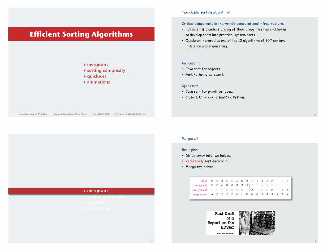
Efficient Sorting Algorithms
‣ mergesort‣ sorting complexity‣ quicksort‣ animations
2
Two classic sorting algorithms
Critical components in the world’s computational infrastructure.
• Full scientific understanding of their properties has enabled usto develop them into practical system sorts.
• Quicksort honored as one of top 10 algorithms of 20th centuryin science and engineering.
Mergesort.
• Java sort for objects.
• Perl, Python stable sort.
Quicksort.
• Java sort for primitive types.
• C qsort, Unix, g++, Visual C++, Python.
‣ mergesort‣ sorting complexity ‣ quicksort‣ animations
3
Basic plan.
• Divide array into two halves.
• Recursively sort each half.
• Merge two halves.
4
Mergesort
Mergesort overview
input
sort left half
sort right half
merge results
M E R G E S O R T E X A M P L E
E E G M O R R S T E X A M P L E
E E G M O R R S A E E L M P T X
A E E E E G L M M O P R R S T X
5
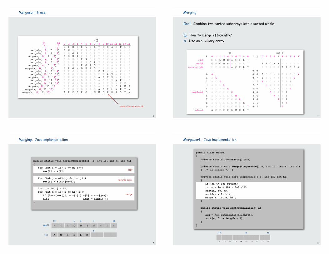
Mergesort trace
Trace of merge results for top-down mergesort
a[] 0 1 2 3 4 5 6 7 8 9 10 11 12 13 14 15 M E R G E S O R T E X A M P L E merge(a, 0, 0, 1) E M R G E S O R T E X A M P L E merge(a, 2, 2, 3) E M G R E S O R T E X A M P L E merge(a, 0, 1, 3) E G M R E S O R T E X A M P L E merge(a, 4, 4, 5) E G M R E S O R T E X A M P L E merge(a, 6, 6, 7) E G M R E S O R T E X A M P L E merge(a, 4, 5, 7) E G M R E O R S T E X A M P L E merge(a, 0, 3, 7) E E G M O R R S T E X A M P L E merge(a, 8, 8, 9) E E G M O R R S E T X A M P L E merge(a, 10, 10, 11) E E G M O R R S E T A X M P L E merge(a, 8, 9, 11) E E G M O R R S A E T X M P L E merge(a, 12, 12, 13) E E G M O R R S A E T X M P L E merge(a, 14, 14, 15) E E G M O R R S A E T X M P E L merge(a, 12, 13, 15 E E G M O R R S A E T X E L M P merge(a, 8, 11, 15) E E G M O R R S A E E L M P T X merge(a, 0, 7, 15) A E E E E G L M M O P R R S T X
lo hi
result after recursive all
Goal. Combine two sorted subarrays into a sorted whole.
Q. How to merge efficiently? A. Use an auxiliary array.
6
Merging
input
copy left
reverse copy right
merged result
final result
a[] aux[]
k 0 1 2 3 4 5 6 7 8 9 i j 0 1 2 3 4 5 6 7 8 9
E E G M R A C E R T - - - - - - - - - -
E E G M R A C E R T E E G M R - - - - -
E E G M R A C E R T E E G M R T R E C A
0 9
0 A 0 8 E E G M R T R E C A
1 A C 0 7 E E G M R T R E C
2 A C E 1 7 E E G M R T R E
3 A C E E 2 7 E G M R T R E
4 A C E E E 2 6 G M R T R E
5 A C E E E G 3 6 G M R T R
6 A C E E E G M 4 6 M R T R
7 A C E E E G M R 5 6 R T R
8 A C E E E G M R R 5 5 T R
9 A C E E E G M R R T 6 5 T
A C E E E G M R R T
7
Merging: Java implementation
A G L O R T S M I H
A G H I L M
i j
k
lo him
aux[]
a[]
public static void merge(Comparable[] a, int lo, int m, int hi) { for (int i = lo; i <= m; i++) aux[i] = a[i]; for (int j = m+1; j <= hi; j++) aux[j] = a[hi-j+m+1]; int i = lo, j = hi; for (int k = lo; k <= hi; k++) if (less(aux[j], aux[i])) a[k] = aux[j--]; else a[k] = aux[i++];}
copy
reverse copy
merge
8
Mergesort: Java implementation
lo m hi
10 11 12 13 14 15 16 17 18 19
public class Merge{ private static Comparable[] aux;
private static void merge(Comparable[] a, int lo, int m, int hi) { /* as before */ } private static void sort(Comparable[] a, int lo, int hi) { if (hi <= lo) return; int m = lo + (hi - lo) / 2; sort(a, lo, m); sort(a, m+1, hi); merge(a, lo, m, hi); }
public static void sort(Comparable[] a) { aux = new Comparable[a.length]; sort(a, 0, a.length - 1); }}
9
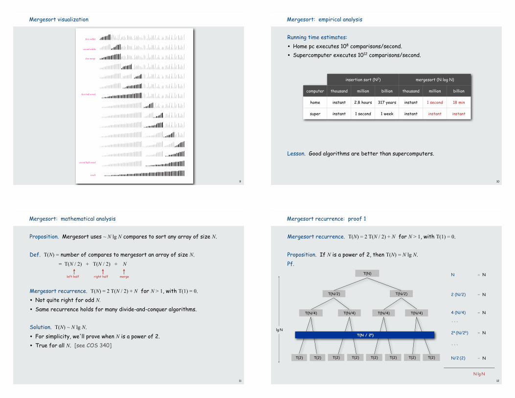
Mergesort visualization
first subfile
second subfile
first merge
first half sorted
second half sorted
result
Visual trace of top-down mergesort with cutoff for small subfiles 10
Mergesort: empirical analysis
Running time estimates:
• Home pc executes 108 comparisons/second.
• Supercomputer executes 1012 comparisons/second.
Lesson. Good algorithms are better than supercomputers.
insertion sort (N2) mergesort (N log N)
computer thousand million billion thousand million billion
home instant 2.8 hours 317 years instant 1 second 18 min
super instant 1 second 1 week instant instant instant
11
Mergesort: mathematical analysis
Proposition. Mergesort uses ~ N lg N compares to sort any array of size N.
Def. T(N) = number of compares to mergesort an array of size N. = T(N / 2) + T(N / 2) + N
Mergesort recurrence. T(N) = 2 T(N / 2) + N for N > 1, with T(1) = 0.
• Not quite right for odd N.
• Same recurrence holds for many divide-and-conquer algorithms.
Solution. T(N) ~ N lg N.
• For simplicity, we'll prove when N is a power of 2.
• True for all N. [see COS 340]
left half right half merge
Mergesort recurrence. T(N) = 2 T(N / 2) + N for N > 1, with T(1) = 0.
Proposition. If N is a power of 2, then T(N) = N lg N.Pf.
12
Mergesort recurrence: proof 1
T(N)
T(N/2)T(N/2)
T(N/4)T(N/4)T(N/4) T(N/4)
T(2) T(2) T(2) T(2) T(2) T(2) T(2)
N
T(N / 2k)
2 (N/2)
2k (N/2k)
N/2 (2)
...
lg N
N lg N
= N
= N
= N
= N
...
T(2)
4 (N/4) = N
Mergesort recurrence. T(N) = 2 T(N / 2) + N for N > 1, with T(1) = 0.
Proposition. If N is a power of 2, then T(N) = N lg N.Pf.
13
Mergesort recurrence: proof 2
T(N) = 2 T(N/2) + N
T(N) / N = 2 T(N/2) / N + 1
= T(N/2) / (N/2) + 1
= T(N/4) / (N/4) + 1 + 1
= T(N/8) / (N/8) + 1 + 1 + 1
. . .
= T(N/N) / (N/N) + 1 + 1 + ... + 1
= lg N
given
divide both sides by N
algebra
apply to first term
apply to first term again
stop applying, T(1) = 0
Mergesort recurrence. T(N) = 2 T(N / 2) + N for N > 1, with T(1) = 0.
Proposition. If N is a power of 2, then T(N) = N lg N.Pf. [by induction on N]
• Base case: N = 1.
• Inductive hypothesis: T(N) = N lg N.
• Goal: show that T(2N) = 2N lg (2N).
14
Mergesort recurrence: proof 3
T(2N) = 2 T(N) + 2N
= 2 N lg N + 2 N
= 2 N (lg (2N) - 1) + 2N
= 2 N lg (2N)
given
inductive hypothesis
algebra
QED
15
Mergesort analysis: memory
Proposition G. Mergesort uses extra space proportional to N.Pf. The array aux[] needs to be of size N for the last merge.
Def. A sorting algorithm is in-place if it uses O(log N) extra memory.Ex. Insertion sort, selection sort, shellsort.
Challenge for the bored. In-place merge. [Kronrud, 1969]
two sorted subarrays
merged array
E E G M O R R S A E E L M P T X
A E E E E G L M M O P R R S T X
16
Mergesort: practical improvements
Use insertion sort for small subarrays.
• Mergesort has too much overhead for tiny subarrays.
• Cutoff to insertion sort for ≈ 7 elements.
Stop if already sorted.
• Is biggest element in first half ≤ smallest element in second half?
• Helps for nearly ordered lists.
Eliminate the copy to the auxiliary array. Save time (but not space) by switching the role of the input and auxiliary array in each recursive call.
Ex. See Program 8.4 or Arrays.sort().
two sorted subarrays
merged array
A E E E E G L M M O P R R S T X
A E E E E G L M M O P R R S T X
biggest element in left half ! smallest element in right half
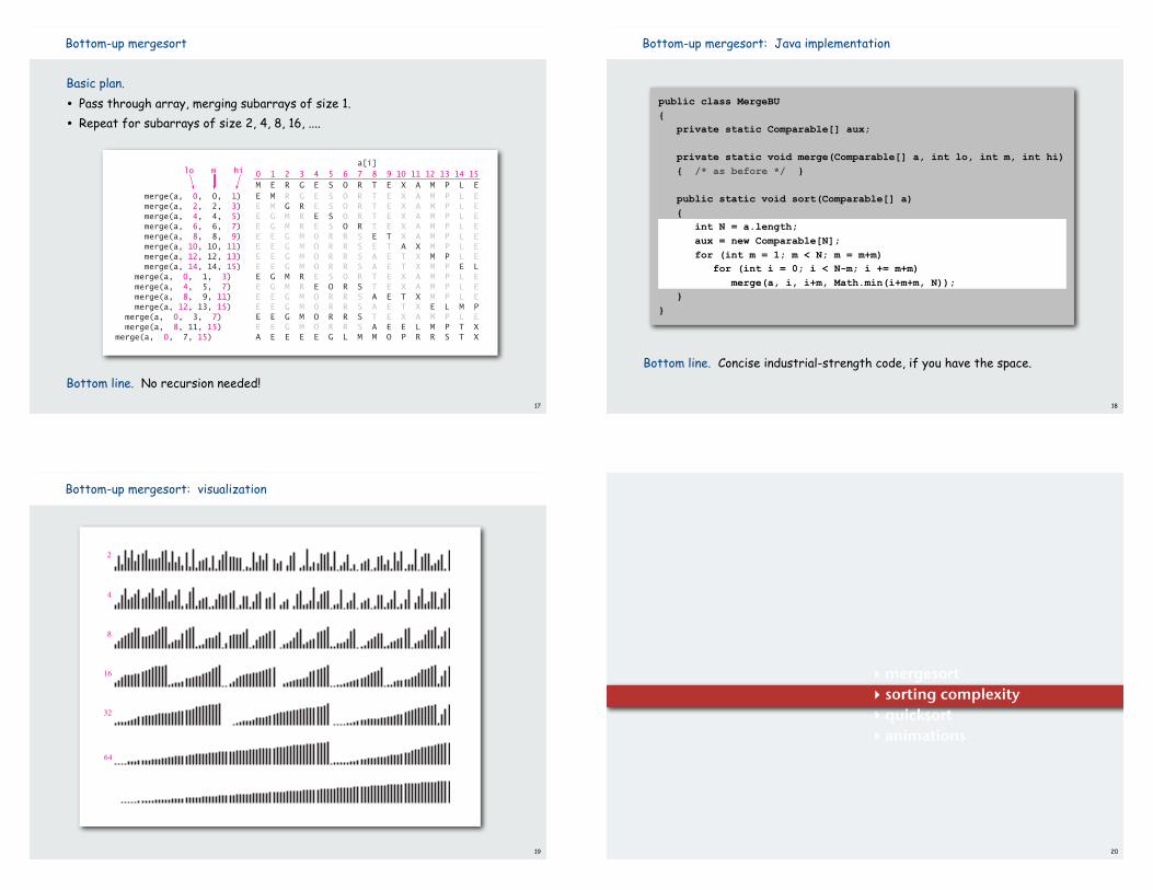
Basic plan.
• Pass through array, merging subarrays of size 1.
• Repeat for subarrays of size 2, 4, 8, 16, ....
Bottom line. No recursion needed!17
Bottom-up mergesort
Trace of merge results for bottom-up mergesort
a[i] 0 1 2 3 4 5 6 7 8 9 10 11 12 13 14 15 M E R G E S O R T E X A M P L E merge(a, 0, 0, 1) E M R G E S O R T E X A M P L E merge(a, 2, 2, 3) E M G R E S O R T E X A M P L E merge(a, 4, 4, 5) E G M R E S O R T E X A M P L E merge(a, 6, 6, 7) E G M R E S O R T E X A M P L E merge(a, 8, 8, 9) E E G M O R R S E T X A M P L E merge(a, 10, 10, 11) E E G M O R R S E T A X M P L E merge(a, 12, 12, 13) E E G M O R R S A E T X M P L E merge(a, 14, 14, 15) E E G M O R R S A E T X M P E L merge(a, 0, 1, 3) E G M R E S O R T E X A M P L E merge(a, 4, 5, 7) E G M R E O R S T E X A M P L E merge(a, 8, 9, 11) E E G M O R R S A E T X M P L E merge(a, 12, 13, 15) E E G M O R R S A E T X E L M P merge(a, 0, 3, 7) E E G M O R R S T E X A M P L E merge(a, 8, 11, 15) E E G M O R R S A E E L M P T X merge(a, 0, 7, 15) A E E E E G L M M O P R R S T X
lo m hi
Bottom line. Concise industrial-strength code, if you have the space.
18
Bottom-up mergesort: Java implementation
public class MergeBU{ private static Comparable[] aux;
private static void merge(Comparable[] a, int lo, int m, int hi) { /* as before */ } public static void sort(Comparable[] a) { int N = a.length; aux = new Comparable[N]; for (int m = 1; m < N; m = m+m) for (int i = 0; i < N-m; i += m+m) merge(a, i, i+m, Math.min(i+m+m, N)); }}
19
Bottom-up mergesort: visualization
2
4
8
16
32
64
Visual trace of bottom-up mergesort
‣ mergesort‣ sorting complexity ‣ quicksort‣ animations
20
21
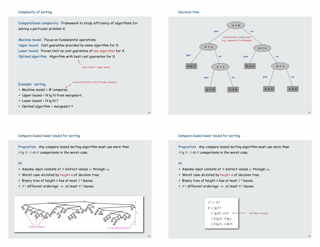
Computational complexity. Framework to study efficiency of algorithms for solving a particular problem X.
Machine model. Focus on fundamental operations.Upper bound. Cost guarantee provided by some algorithm for X.Lower bound. Proven limit on cost guarantee of any algorithm for X.Optimal algorithm. Algorithm with best cost guarantee for X.
Example: sorting.
• Machine model = # compares.
• Upper bound = N lg N from mergesort.
• Lower bound = N lg N ?
• Optimal algorithm = mergesort ?
lower bound ~ upper bound
access information only through compares
Complexity of sorting
22
Decision tree
b < c
yes no
a < c
yes no
a < c
yes no
a c b c a b
b a c
a < b
yes no
code between comparisons(e.g., sequence of exchanges)
a b c b < c
yes no
b c a c b a
23
Compare-based lower bound for sorting
Proposition. Any compare-based sorting algorithm must use more thanN lg N - 1.44 N comparisons in the worst-case.
Pf.
• Assume input consists of N distinct values a1 through aN.
• Worst case dictated by height h of decision tree.
• Binary tree of height h has at most 2 h leaves.
• N ! different orderings ⇒ at least N ! leaves.
at least N! leaves
Compare tree boundsno more than 2h leaves
h
24
Compare-based lower bound for sorting
Proposition. Any compare-based sorting algorithm must use more thanN lg N - 1.44 N comparisons in the worst-case.
Pf.
• Assume input consists of N distinct values a1 through aN.
• Worst case dictated by height h of decision tree.
• Binary tree of height h has at most 2 h leaves.
• N ! different orderings ⇒ at least N ! leaves.
2 h ≥ N !
h ≥ lg N !
≥ lg (N / e) N
= N lg N - N lg e
≥ N lg N - 1.44 N
Stirling's formula
25
Complexity of sorting
Machine model. Focus on fundamental operations.Upper bound. Cost guarantee provided by some algorithm for X.Lower bound. Proven limit on cost guarantee of any algorithm for X.Optimal algorithm. Algorithm with best cost guarantee for X.
Example: sorting.
• Machine model = # compares.
• Upper bound = N lg N from mergesort.
• Lower bound = N lg N - 1.44 N.
• Optimal algorithm = mergesort.
First goal of algorithm design: optimal algorithms.
26
Complexity results in context
Other operations? Mergesort optimality is only about number of compares.
Space?
• Mergesort is not optimal with respect to space usage.
• Insertion sort, selection sort, and shellsort are space-optimal.
• Is there an algorithm that is both time- and space-optimal?
Lessons. Use theory as a guide.Ex. Don't try to design sorting algorithm that uses ½ N lg N compares.
27
Complexity results in context (continued)
Lower bound may not hold if the algorithm has information about
• The key values.
• Their initial arrangement.
Partially ordered arrays. Depending on the initial order of the input,we may not need N lg N compares.
Duplicate keys. Depending on the input distribution of duplicates,we may not need N lg N compares.
Digital properties of keys. We can use digit/character comparisons instead of key comparisons for numbers and strings.
insertion sort requires O(N) compares onan already sorted array
stay tuned for 3-way quicksort
stay tuned for radix sorts
‣ mergesort‣ sorting complexity ‣ quicksort‣ animations
28
29
Quicksort
Basic plan.
• Shuffle the array.
• Partition so that, for some i
- element a[i] is in place- no larger element to the left of i
- no smaller element to the right of i
• Sort each piece recursively.Sir Charles Antony Richard Hoare
1980 Turing Award
Quicksort overview
input
shuffle
partition
sort left
sort right
result
Q U I C K S O R T E X A M P L E
E R A T E S L P U I M Q C X O K
E C A I E K L P U T M Q R X O S
A C E E I K L P U T M Q R X O S
A C E E I K L M O P Q R S T U X
A C E E I K L M O P Q R S T U X
not greater not less
partitioning element
Quicksort partitioning
Basic plan.
• Scan from left for an item that belongs on the right.
• Scan from right for item item that belongs on the left.
• Exchange.
• Continue until pointers cross.
30
Partitioning trace (array contents before and after each exchange)
a[i] i j 0 1 2 3 4 5 6 7 8 9 10 11 12 13 14 15
-1 15 E R A T E S L P U I M Q C X O K
1 12 E R A T E S L P U I M Q C X O K
1 12 E C A T E S L P U I M Q R X O K
3 9 E C A T E S L P U I M Q R X O K
3 9 E C A I E S L P U T M Q R X O K
5 5 E C A I E S L P U T M Q R X O K
5 5 E C A I E K L P U T M Q R X O S
E C A I E K L P U T M Q R X O S
initial values
scan left, scan right
exchange
scan left, scan right
exchange
scan left, scan right
final exchange
result
v
private static int partition(Comparable[] a, int lo, int hi){ int i = lo - 1; int j = hi; while(true) {
while (less(a[++i], a[hi])) if (i == hi) break;
while (less(a[hi], a[--j])) if (j == lo) break;
if (i >= j) break; exch(a, i, j); }
exch(a, i, hi); return i;}
31
Quicksort: Java code for partitioning
swap with partitioning item
check if pointers cross
find item on right to swap
find item on left to swap
swap
return index of item now known to be in place
Quicksort partitioning overview
i
v v
j
v
v
lo hi
lo hi
v v
j
before
during
after
v
32
Quicksort: Java implementation
public class Quick{ public static void sort(Comparable[] a) { StdRandom.shuffle(a); sort(a, 0, a.length - 1); }
private static void sort(Comparable[] a, int lo, int hi) { if (hi <= lo) return; int i = partition(a, lo, hi); sort(a, lo, i-1); sort(a, i+1, hi); }}
Quicksort trace
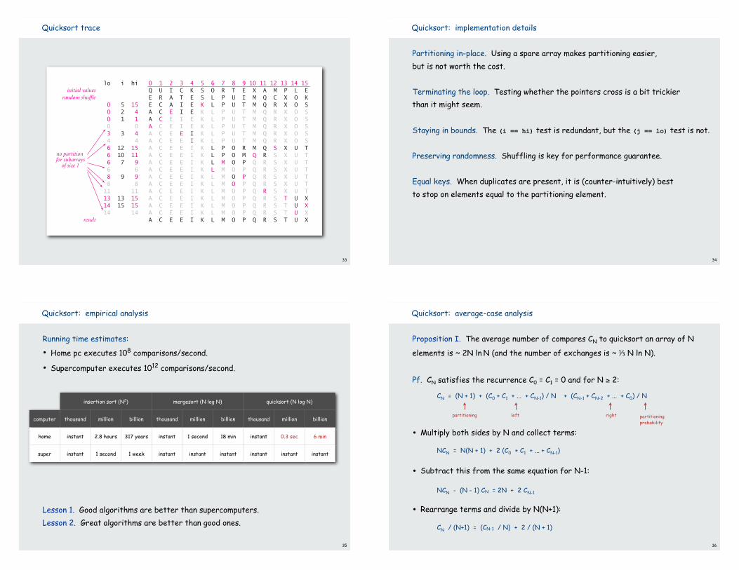
33
Quicksort trace (array contents after each partition)
lo i hi 0 1 2 3 4 5 6 7 8 9 10 11 12 13 14 15 Q U I C K S O R T E X A M P L E E R A T E S L P U I M Q C X O K 0 5 15 E C A I E K L P U T M Q R X O S 0 2 4 A C E I E K L P U T M Q R X O S 0 1 1 A C E I E K L P U T M Q R X O S 0 0 A C E I E K L P U T M Q R X O S 3 3 4 A C E E I K L P U T M Q R X O S 4 4 A C E E I K L P U T M Q R X O S 6 12 15 A C E E I K L P O R M Q S X U T 6 10 11 A C E E I K L P O M Q R S X U T 6 7 9 A C E E I K L M O P Q R S X U T 6 6 A C E E I K L M O P Q R S X U T 8 9 9 A C E E I K L M O P Q R S X U T 8 8 A C E E I K L M O P Q R S X U T 11 11 A C E E I K L M O P Q R S X U T 13 13 15 A C E E I K L M O P Q R S T U X 14 15 15 A C E E I K L M O P Q R S T U X 14 14 A C E E I K L M O P Q R S T U X A C E E I K L M O P Q R S T U X
initial valuesrandom shuffle
result
no partition for subarrays
of size 1
34
Quicksort: implementation details
Partitioning in-place. Using a spare array makes partitioning easier,but is not worth the cost.
Terminating the loop. Testing whether the pointers cross is a bit trickierthan it might seem.
Staying in bounds. The (i == hi) test is redundant, but the (j == lo) test is not.
Preserving randomness. Shuffling is key for performance guarantee.
Equal keys. When duplicates are present, it is (counter-intuitively) bestto stop on elements equal to the partitioning element.
35
Quicksort: empirical analysis
Running time estimates:
• Home pc executes 108 comparisons/second.
• Supercomputer executes 1012 comparisons/second.
Lesson 1. Good algorithms are better than supercomputers.Lesson 2. Great algorithms are better than good ones.
insertion sort (N2) mergesort (N log N) quicksort (N log N)
computer thousand million billion thousand million billion thousand million billion
home instant 2.8 hours 317 years instant 1 second 18 min instant 0.3 sec 6 min
super instant 1 second 1 week instant instant instant instant instant instant
Proposition I. The average number of compares CN to quicksort an array of N
elements is ~ 2N ln N (and the number of exchanges is ~ ⅓ N ln N).
Pf. CN satisfies the recurrence C0 = C1 = 0 and for N ≥ 2:
• Multiply both sides by N and collect terms:
• Subtract this from the same equation for N-1:
• Rearrange terms and divide by N(N+1):
36
Quicksort: average-case analysis
CN = (N + 1) + (C0 + C1 + ... + CN-1) / N + (CN-1 + CN-2 + ... + C0) / N
NCN = N(N + 1) + 2 (C0 + C1 + ... + CN-1)
partitioning right partitioningprobability
left
NCN - (N - 1) CN = 2N + 2 CN-1
CN / (N+1) = (CN-1 / N) + 2 / (N + 1)
• From before:
• Repeatedly apply above equation:
• Approximate by an integral:
• Finally, the desired result:
37
Quicksort: average-case analysis
CN / (N + 1) = CN-1 / N + 2 / (N + 1)
= CN-2 / (N - 1) + 2/N + 2/(N + 1)
= CN-3 / (N - 2) + 2/(N - 1) + 2/N + 2/(N + 1)
= 2 ( 1 + 1/2 + 1/3 + . . . + 1/N + 1/(N + 1) )
CN ≈ 2(N + 1) ( 1 + 1/2 + 1/3 + . . . + 1/N )
= 2(N + 1) HN ≈ 2(N + 1) ∫1N dx/x
CN ≈ 2(N + 1) ln N ≈ 1.39 N lg N
CN / (N+1) = CN-1 / N + 2 / (N + 1)
38
Quicksort: summary of performance characteristics
Worst case. Number of compares is quadratic.
• N + (N-1) + (N-2) + … + 1 ~ N2 / 2.
• More likely that your computer is struck by lightning.
Average case. Number of compares is ~ 1.39 N lg N.
• 39% more compares than mergesort.
• But faster than mergesort in practice because of less data movement.
Random shuffle.
• Probabilistic guarantee against worst case.
• Basis for math model that can be validated with experiments.
Caveat emptor. Many textbook implementations go quadratic if input:
• Is sorted or reverse sorted
• Has many duplicates (even if randomized!) [stay tuned]
39
Quicksort: practical improvements
Median of sample.
• Best choice of pivot element = median.
• Estimate true median by taking median of sample.
Insertion sort small files.
• Even quicksort has too much overhead for tiny files.
• Can delay insertion sort until end.
Optimize parameters.
• Median-of-3 random elements.
• Cutoff to insertion sort for ≈ 10 elements.
Non-recursive version.
• Use explicit stack.
• Always sort smaller half first.
guarantees O(log N) stack size
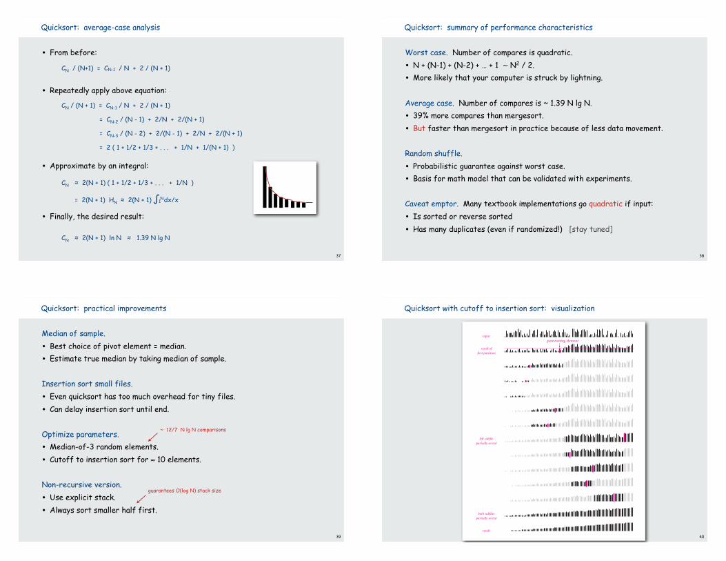
~ 12/7 N lg N comparisons
Quicksort with cutoff to insertion sort: visualization
40
input
result offirst partition
both subfilespartially sorted
result
left subfilepartially sorted
Quicksort with cutoff for small subfiles
partitioning element
‣ mergesort‣ sorting complexity ‣ quicksort‣ animations
41 42
Mergesort animation
merge in progress output auxiliary array
done merge in progress inputuntouched
43
Mergesort animation
44
Botom-up mergesort animation
merge in progress output auxiliary array
this pass merge in progress inputlast pass
45
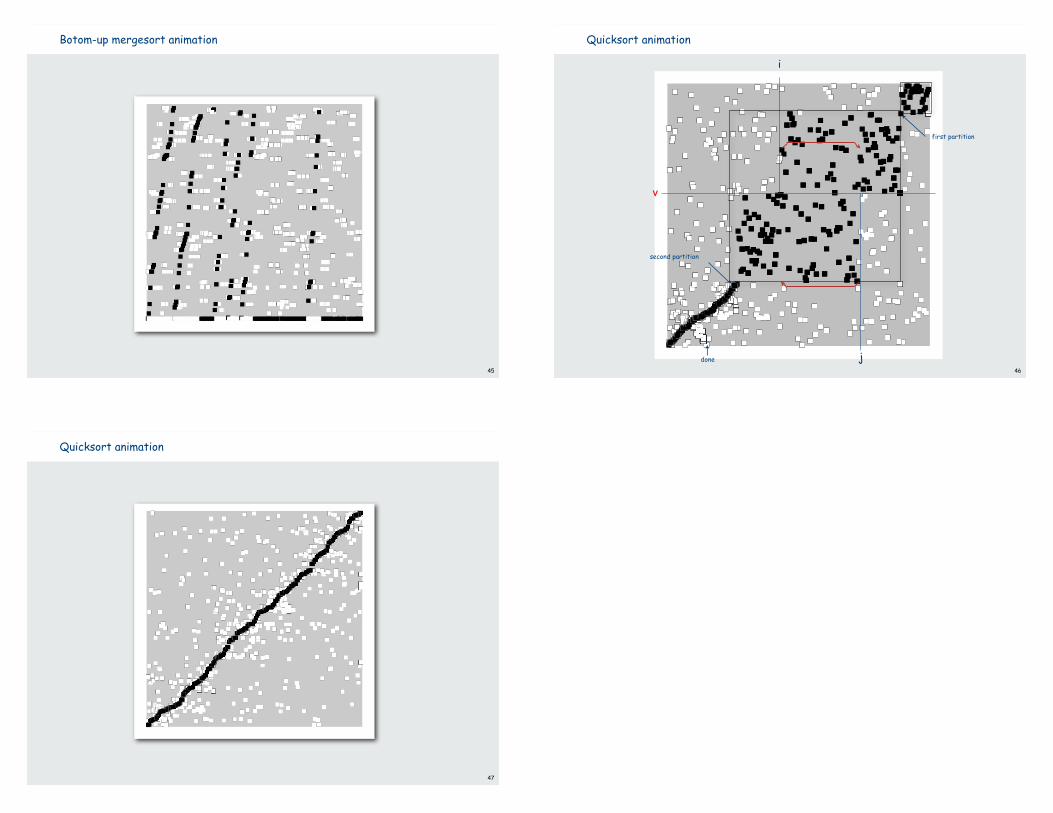
Botom-up mergesort animation Quicksort animation
46
j
i
v
done
first partition
second partition
47
Quicksort animation
Recommended