I.J. Intelligent Systems and Applications, 2013, 03, 37-49
Published Online February 2013 in MECS (http://www.mecs-press.org/)
DOI: 10.5815/ijisa.2013.03.04
Copyright © 2013 MECS I.J. Intelligent Systems and Applications, 2013, 03, 37-49
Efficient Data Clustering Algorithms:
Improvements over Kmeans
Mohamed Abubaker, Wesam Ashour
Dept. of Computer Engineering, Islamic University of Gaza, Gaza, Palestine
[email protected];[email protected]
Abstract— This paper presents a new approach to
overcome one of the most known disadvantages of the
well-known Kmeans clustering algorithm. The
problems of classical Kmeans are such as the problem
of random init ialization of prototypes and the
requirement of predefined number of clusters in the
dataset. Randomly in itialized prototypes can often yield
results to converge to local rather than global optimum.
A better result of Kmeans may be obtained by running
it many times to get satisfactory results. The proposed
algorithms are based on a new novel definition of
densities of data points which is based on the k-nearest
neighbor method. By this definit ion we detect noise and
outliers which affect Kmeans strongly, and obtained
good initial prototypes from one run with automatic
determination of K nu mber of clusters. This algorithm
is referred to as Efficient In itializat ion of Kmeans (EI-
Kmeans). Still Kmeans algorithm used to cluster data
with convex shapes, similar sizes, and densities. Thus
we develop a new clustering algorithm called Efficient
Data Clustering Algorithm (EDCA) that uses our new
definit ion of densities of data points. The results show
that the proposed algorithms improve the data clustering
by Kmeans. EDCA is able to detect clusters with
different non-convex shapes, different sizes and
densities.
Index Terms— Data Clustering, Random In itializat ion,
Kmeans, K-Nearest Neighbor, Density, Noise, Outlier,
Data Point
I. Introduction
Data clustering techniques are an important aspect
used in many fields such as data min ing [1], pattern
recognition and pattern classification [2], data
compression [3], machine learn ing [4], image analysis
[5], and bioinformatics [6].
The purpose of clustering is to group data points into
clusters in which the similar data points are grouped in
the same cluster while d issimilar data points are in
different clusters. The high quality of clustering is to
obtain high intra-cluster similarity and low inter-cluster
similarity.
The clustering problems can be categorized into two
main types: fuzzy clustering and hard clustering. In
fuzzy clustering, data points can belong to more than
one cluster with probabilities [7] which indicate the
strength of relationships between the data points and a
particular cluster.
One of the most widely used fuzzy clustering
algorithms is fuzzy c-mean algorithm [8]. In hard
clustering, data points are divided into distinct clusters,
where each data point can belong to one and only one
cluster. The hard clustering is subdivided into
hierarchical and part itional algorithms. Hierarchical
algorithms create nested relationships of clusters which
can be represented as a tree structure called dendrogram
[9]. These algorithms can be div ided into agglomerative
and divisive hierarchical algorithms. The agglomerative
hierarchical clustering starts with each data point in a
single cluster. Then it repeats merging the similar pairs
of clusters until all of the data points are in one cluster,
such as complete linkage clustering [10] and single
linkage clustering [11]. The divisive hierarchical
algorithm reverses the operations of agglomerative
clustering, it starts with all data points in one cluster and
repeats splitting large clusters into smaller ones until
each data point belong to a single cluster such as
DIANA clustering algorithm [12].
Partit ional clustering algorithm d ivides the data set
into a set of disjoint clusters such as Kmeans [13], PAM
[12] and CLARA [12].
One of the most well-known unsupervised learning
algorithms for clustering datasets is Kmeans algorithm
[12]. The Kmeans clustering is the most widely used
[14] due to its simplicity and efficiency in various fields.
It is also considered as the top ten algorithms in data
mining [15]. The Kmeans algorithm works as follows:
1. Select a set of initial k prototypes or means
throughout a data set, where k is a user-defined
parameter represents the number of clusters in the
data set.
2. Assign each data point in a data set to its nearest
prototypes m.
3. Update each prototype according to the average of
data points assigned to it.
4. Repeat step 2 and 3 until convergence.
38 Efficient Data Clustering Algorithms: Improvements over Kmeans
Copyright © 2013 MECS I.J. Intelligent Systems and Applications, 2013, 03, 37-49
2
1
1
k
i Cxi
i
mxn
J (1)
The Kmeans updates their prototypes iteratively to
minimize the following criterion function:
Where data set D contains n data points or objects
nxx ,...,1such as each data point is d dimensional vector
in Rd, and mi is the prototype of cluster Ci, and k is the
given number of clusters.
The main advantages of Kmeans algorithm are its
simplicity to be implemented and its efficiency.
However, it has several drawbacks:
The number of clusters in a g iven data set should
be known in advance.
The result strongly depends on the initial
prototypes.
It is applicable when the mean of data is defined.
Sensitivity to noise and outliers.
Dead prototypes or Empty clusters.
Converge to local optima.
It is defined for globular shaped, similar size and
density clusters.
A number of kernel methods have been proposed in
recent years [16-19] to increase the separable of clusters.
In the kernel Kmeans algorithm all data points are
mapped, before clustering, to a higher d imensional
feature space by using a kernel function. Then the
Kmeans algorithm is applied in the new feature space to
identify clusters. Recently, [20,21] p roposed a novel of
new clustering algorithms that converge to a better
solution (less prone to finding a local minimum because
of poor initialization) than both standard Kmeans and a
mixture of experts trained using the EM algorithm.
In this paper, we modify the non-parametric density
estimation based on kn-nearest neighbors algorithm [22].
So, our proposed algorithm is robust to noise and
outliers, automatically detects the number of clusters in
the data set, and selects the most representative dense
prototypes to be initial prototypes even if the clusters
are in different shapes with different densities.
To compute the kn-nearest neighbors algorithm of a
data point Dxi , we center a ball cell about xi and let it
grows until it captures the predefined number kn of data
points. Let ))(( ixNR represents the radius of the ball
which is the distance from xi to its farthest neighbor in
its )( ixN , where )( ixN represents a set of data points in
the kn neighborhood of xi. Then the density of xi is
defined as [22,23]:
)))(((.)(
i
ni xNRVn
kxden (2)
Where V(r) represents the volume of ball of rad ius r
in Rd, and )2/(/2)( 2/ ddrrV dd .
The clustering algorithms that are based on
estimating the densities of data points are known as
density-based. One of the basic density based clustering
algorithm is DBSCAN [24]. It defines the density by
counting the number of data points in a region specified
by a predefined rad ius known as Eps around the data
point. If a data point has a number greater than or equal
to predefined min imum points, then this point is treated
as a core point. Non-core data points that do not have a
core data point within the predefined radius are treated
as noise. Then the clusters are formed around the core
data points and are defined as a set of density-connected
data points that is maximal with respect to density
reachability. DBSCAN may behave poorly due it is
weak definition o f data points’ densities and it is
globally predefined parameters.
II. Related Works
There are several p rototypes initializat ion methods
have been introduced for the classical Kmeans
algorithms. In [25] the prototypes are chosen randomly
from the data set which considers the simplest and most
common init ialization method. The Minmax [26] selects
the first prototype randomly m1 then the ith
prototype mi
is selected to be the data points with largest minimum
distance to the previously selected prototypes. One of
the drawbacks of this method is that it is sensitive to
outliers thus it selects the outliers in the data set.
Kmeans++ [27] in which the first prototype mi is
selected randomly m1 then the ith
prototype is selected to
be Dx ' with probability of Dx xdxd 22 )()'( ,
where d(x) denotes the shortest distance from data point x to the closet prototype already chosen. Al-Daoud in
[28] p roposed an algorithm to initialize the prototypes
of Kmeans which finds a set of medians extracted from
the dimension with maximum variance to be the init ial
prototypes. The use of median in this method makes the
algorithm sensitive to outliers. Gan, Ma, and Wu in [9]
introduced a valid ity measure to determine the number
of clusters in Kmeans algorithm. This method depends
on calculating the intra-cluster distances Mintra which is
defined as in (1) and the inter-cluster distances Minter which is the minimum distance between pair of
prototypes among all prototypes. Then the validity
measure is defined as: erra MMV intint . Obviously a
good result shall have a small intra-cluster distances and
a large inter-cluster distances, thus V is min imized. To
determine V we shall apply Kmeans algorithm from k=2
up to Kmax and for each we calculate the validity
measure and choose the k that corresponds to the
minimum value of V.
III. Motivations
The Kmeans algorithm considered as one of the top
ten algorithms in data mining [15]. A lot of researches
and studies have been proposed due to its simplicity and
efficiency. These efforts have focused on finding
Efficient Data Clustering Algorithms: Improvements over Kmeans 39
Copyright © 2013 MECS I.J. Intelligent Systems and Applications, 2013, 03, 37-49
possible solutions to one or more of the limitations that
have been identified previously. One of the solutions to
the initial p rototypes sensitivity can be found in [29]
where they defined new criterion functions for Kmeans
and they proposed three new algorithms: weighted
Kmeans, inverse weighted Kmeans [30] and inverse
exponential Kmeans [31]. Other improvements of
Kmeans focus on its efficiency where the complexity of
Kmeans involves the data set size, number of
dimensions, number of clusters and the number of
iteration to be converged. There are many works to
reduce the computational load and make it more fast
such as in [32-34]. Asgharbeygi and Maleki in [23]
proposed a new distance metric which is the geodesic
distance to ensure resistance to outliers. Several works
have been introduced to extend the use of means for
numerical variables, thus Kmeans can deal with
categorical variables such as in [35,36].
Our proposed EI-Kmeans algorithm focuses on
classical Kmeans itself. We want to in itialize prototypes
from the first run on compete positions throughout the
data set that yields good results. EI-Kmeans also solves
one of the most difficult problems in the data clustering
which is the determination of the number of clusters in
the data set in advance. The determination of number of
clusters depends on our new defined density of data
points that can eliminate noise and outliers from the
data set. The proposed EDCA tries to benefit from the
proposed EI-Kmeans to develop a new clustering
algorithm that is able to detect clusters with different
non-convex shapes, different sizes and densities in
which Kmeans cannot give good results in these types
of data sets.
IV. Proposed Algorithms
The proposed algorithms define a new definition for
the density of data points throughout the data set. This
new defin ition mentions the drawback of (2) which is
based on kn-nearest neighbors density estimation
[22,23]. EI-Kmeans calculates the density of each data
point in the given data set, and then it sorts the data
points in descending order according to their densities.
The first densest point is selected as the first prototype.
Then the list of sorted data points is investigated to get
the next candidate prototypes. However, we shall take
care that the selected prototype does not have a direct
connectivity with the previously selected prototypes.
We define two versions of EI-Kmeans algorithm. The
first version takes kn the number of nearest neighbors,
and the number of clusters k in the data set as input
parameters. Then the sorted list of data points is
investigated until the number of obtained prototypes
reached the specified k then the algorithm is aborted.
The second version takes kn the number of nearest
neighbors as the only input parameter and obtains both
the number of clusters and the prototypes in parallel.
We also propose another version which is an
improvement of our second version. However, this third
version considers as a new clustering algorithm. This
new algorithm is referred to as Efficient Data Clustering
Algorithm (EDCA).
The following subsections describe the proposed
algorithms in details:
4.1 New definition of density
We derived our new formula of density based on the
drawbacks of (2).
To illustrate this drawback, let us consider the simple
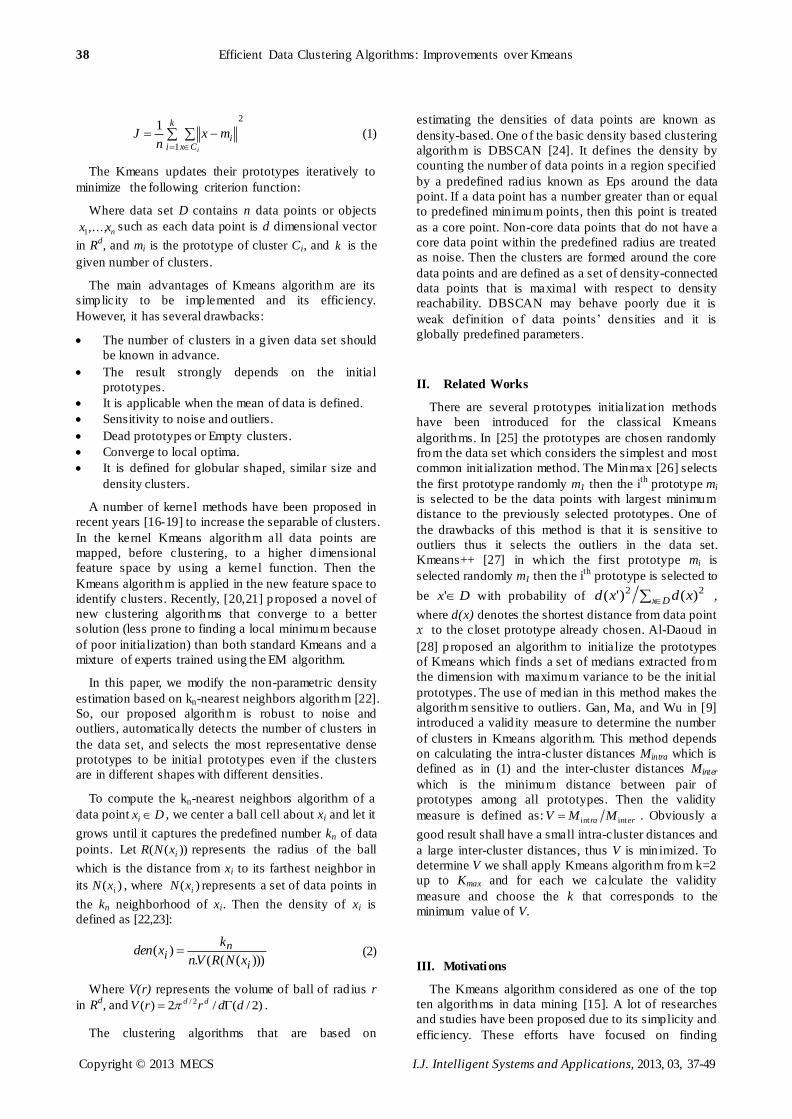
data set example in which it contains 33 data points
distributed as shown in Figure 1. Assume grid is a unit
distance.
Fig. 1: Illustration example
We want to examine the density of the numbered data
points from 1 to 5 with respect to kn=6 including the
examined data point. By applying (2), the density of
data points 1, 2, and 3 is the same and equals to 0.007.
And the density of data points 4 and 5 equals to 0.029.
It is obvious that each numbered data point has a
different density with data point number 5 is the densest
one and data point number 1 has a least density. It is
true that (2) does not take into account the actual
number of data points within ball cell about examined
data points with respect to kn. If we try to engage the
sum of Euclidean distances from the examined data
point to all of its neighbors defined by kn. Then we have
the formula for density of data points:
)( ),()( xNyt yxdNxden where Nt represents the
actual number of data points in the neighborhood of
data point x with respect to kn, N(x) is a set of data
points in the neighborhood of data point x with respect
to kn, and d(x,y) is the Euclidean distance from data
point x to data point y . Then the density of point
numbered 1 is 0.55, density of data point numbered 2 is
40 Efficient Data Clustering Algorithms: Improvements over Kmeans
Copyright © 2013 MECS I.J. Intelligent Systems and Applications, 2013, 03, 37-49
0.88, density of data point numbered 3 is 0.72, density
of data point numbered 4 is 1.11, and density of data
point numbered 5 is 0.93. Again this formula fails to
specify the density of data points accurately. Then we
put our new formula of density based on the density
estimation of (2). The density of data point x is defined
as:
)(
),(.)(
xNy
t
nyxdVn
Nxdensity (3)
Where Nt represents the actual number of data points
in the neighborhood of data point x with respect to kn, n
is the total number of data points in the data set, V is the
volume defined as in (2), and Nn(x) is a set of closest kn
neighbors to point x.
According to (3), the density of point 1 is 0.66, the
density of data point 2 is 1.06, the density of data point
3 is 0.87, the density of data point 4 is 5.34, and the
density of data point 5 is 8.02.
4.2 EI-Kmeans algorithm
Let D be a data set of n d-dimensional data
points nxx ,...,1 . Then we want to find the best candidate
data points to be the initialized prototypes. Thus we can
perform the Kmeans clustering algorithm on the given
data set for obtaining a good result of clustering data
points. The proposed algorithm solves the problem of
considering the number of clusters of the data set in
advance. And it solves the problem of bad init ialized
prototypes that may y ield the algorithm to converge to
local optima or to get empty clusters [29]. EI-Kmeans
algorithm uses our new formula of density defined in
(3). EI-Kmeans searches the data set for the densest
points which are strong candidate prototypes. We take
care that the given data set may contain different
clusters that have different densities, thus a number of
densest points can present in the same cluster.
Let the set P consists of initial prototypes of data set
and it is in itialized to be empty. We compute the density
for each data point in the data set. Then we sort the data
point according to their densities in descending order.
The first data point in this sorted list is the densest data
point in the entire data set. We choose this point to be
the first in itialized prototypes. Then the set P consists of
this prototype. Now we want to examine the next
densest data point in the sorted list in order. To avoid
selecting prototypes that resides in the same cluster. We
test the connectivity between the examined data point
and each prototype in the set P. Thus, if there is no path
between examined data point and each prototype in the
set P, this examined data point is inserted in the set P.
Then the next one which is not examined data point in
the sorted list is tested to be an available prototype or
not. This procedure is repeated until we obtain the
desired prototypes. The path between pairs of data
points is calculated, if exists, as a proactive scheme this
means that we build a proximity matrix o f 0 and 1
where 0 means that there is no direct connectivity
between two data points and 1 means there is a direct
connectivity between two data points. This is calculated
according to a threshold value ɛ which is calculated
dynamically for the given data set. The value ɛ defines
the radius of the region in which direct connectivity is
considered. We compute ɛ for the given data set D as
follows:
d
d
n
n
dkxxprod1
.
)15.0(.)).min()(max(
(4)
Where max(x) treats the columns of x as vectors, and
returns a row vector containing the maximum element
from each co lumn. The same th ing for min but it returns
the min imum element for each column. And prod(A)
returns the product of elements of vector A.
Then we use the connectivity proximity matrix to
find a path between pairs of data points. If the value of
the path is infinity then there is no path between the
given pairs of data points. The following two
subsections describe two versions of EI-Kmeans
algorithm.
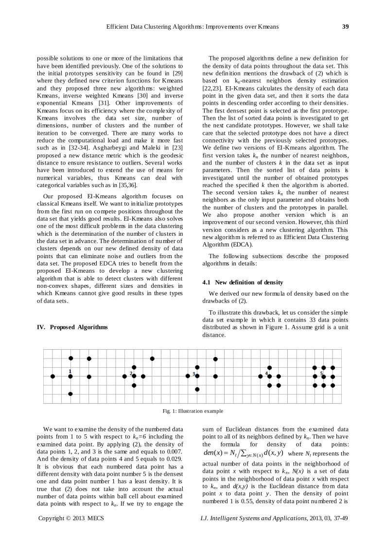
4.2.1 EI-Kmeans version 1
EI-Kmeans_V1(kn,k)
1 Begin initialize kn, k, P={ }, G={ }, n
2 for i = 1 to n 3 PDi ← density(xi) 4 end_for
5 G ← sort(PD)
6 P1 ← G1
7 j = 1
8 do j ← j + 1
9 if there is no path between Gj and each
element in P
10 Append Gj to P
11 end_if
12 Until P contains k elements
13 Return P
14 end
Fig. 2: EI-Kmeans algorithm version 1
The proposed version 1 o f the algorithm takes two
input parameters which are the kn number of nearest
neighbors and k the number of clusters in the data set.
The output is the set of k prototypes. Figure 2 shows the
algorithm. The first step initializes two empty sets P
and G. The set P contains indexes of chosen prototypes
and the set G is a sorted list of data points’ indexes
according to the density in descending order. And n is
the number of data points in the D data set. For each
data point in the data set, we compute the density of this
data point according to (3) and store the results in an
array list of Po int Density (PD). Line 5 of the algorithm
sorts obtained densities in descending order and put the
result in the set G. Line 6 means that the first element in
the set G is selected as a first prototype. The first
Efficient Data Clustering Algorithms: Improvements over Kmeans 41
Copyright © 2013 MECS I.J. Intelligent Systems and Applications, 2013, 03, 37-49
element of G is the index of the densest data point in the
data set. Then a counter j points to the second densest
data point and it is incremented by one for each loop
throughout lines 8 to 12. In each loop we test the
pointed data point in the set G if there is no path
between this data point and each prototype in set P, we
append the index of this data point to the set P.
Otherwise, we increment the counter j to test the next
data point in G. These steps are repeated until k
prototypes are found. Then the algorithm breaks and
returns the k prototypes which they are considered the
init ial prototypes for the Kmeans clustering algorithm.
Thus after obtaining these k prototypes, we run the
standard Kmeans clustering algorithm.
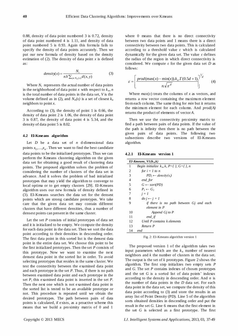
4.2.2 EI-Kmeans version 2
The second version of EI-Kmeans takes only one
input parameter which is the kn number of nearest
neighbors. Figure 3 p resents the EI-Kmeans algorithm.
If we mention our algorithm, then we mean the second
version. Otherwise, it is stated explicitly.
EI-Kmeans_V2(kn)
1 Begin initialize kn, k←0, P={ }, G={ }, n
2 for i = 1 to n
3 PDi ← density(xi)
4 end_for
5 G ← sort(PD)
6 P1 ← G1
7 for each data point in data set D
8 Np ← compute the number of points within
radius ɛ
9 if Np < kn
10 Mark this point as Noise
11 end_if
12 end_for
13 j = 1
14 do j ← j + 1
15 if Gj is not marked as noise
16 if there is no path between Gj and each
element in P
17 Append Gj to P
18 k ← k + 1
19 end_if
20 end_if
21 Until j = n
22 Return P and k
23 end
Fig. 3: EI-Kmeans algorithm version 2
We add a defin ition for noise points. These points are
excluded from the computations and they often reside in
the bottom of the set G. We investigate all of the data
points in the set G except the points marked as noise.
The algorithm finds all of the possible prototypes in the
entire data set. Thus the number of found prototypes
indicates the number of clusters in the data set. The
resulted prototypes are used as the initial prototypes for
clustering the data set using Kmeans algorithm.
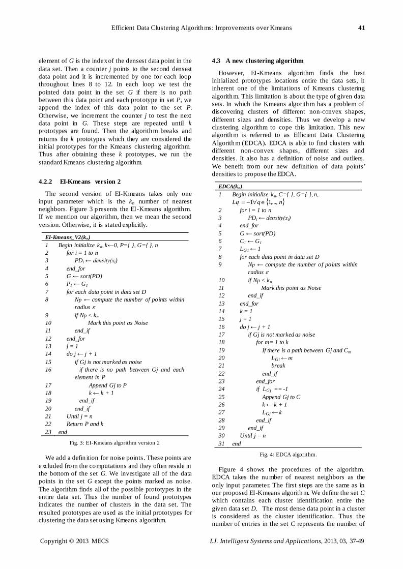
4.3 A new clustering algorithm
However, EI-Kmeans algorithm finds the best
init ialized prototypes locations entire the data sets, it
inherent one of the limitat ions of Kmeans clustering
algorithm. This limitation is about the type of given data
sets. In which the Kmeans algorithm has a problem of
discovering clusters of different non-convex shapes,
different sizes and densities. Thus we develop a new
clustering algorithm to cope this limitation. This new
algorithm is referred to as Efficient Data Clustering
Algorithm (EDCA). EDCA is able to find clusters with
different non-convex shapes, different sizes and
densities. It also has a definition of noise and outliers.
We benefit from our new definition of data points’
densities to propose the EDCA.
EDCA(kn)
1 Begin initialize kn, C={ }, G={ }, n,
Lq nq ,...,11
2 for i = 1 to n
3 PDi ← density(xi)
4 end_for
5 G ← sort(PD)
6 C1 ← G1
7 LG1 ← 1
8 for each data point in data set D
9 Np ← compute the number of points within
radius ɛ
10 if Np < kn
11 Mark this point as Noise
12 end_if
13 end_for
14 k = 1
15 j = 1
16 do j ← j + 1
17 if Gj is not marked as noise
18 for m= 1 to k
19 If there is a path between Gj and Cm
20 LGj ← m
21 break
22 end_if
23 end_for
24 if LGj == -1
25 Append Gj to C
26 k ← k + 1
27 LGj ← k
28 end_if
29 end_if
30 Until j = n
31 end
Fig. 4: EDCA algorithm.
Figure 4 shows the procedures of the algorithm.
EDCA takes the number of nearest neighbors as the
only input parameter. The first steps are the same as in
our proposed EI-Kmeans algorithm. We define the set C
which contains each cluster identification entire the
given data set D. The most dense data point in a cluster
is considered as the cluster identification. Thus the
number of entries in the set C represents the number of
42 Efficient Data Clustering Algorithms: Improvements over Kmeans
Copyright © 2013 MECS I.J. Intelligent Systems and Applications, 2013, 03, 37-49
clusters in the data set. Initially, C is empty. We denote
the cluster label of the data point by Lq. Init ially all data
points are assigned the label of -1 to indicate unassigned
data point, that is Lq nq ,...,11 . EDCA appends
the index of the densest data point according to (3) to
the set C to be the first cluster identification and we
label it to be in the first cluster. We use this point as the
first reference to expand the cluster. Each data point in
the data set is examined in order as in the set G which is
a set of data points’ indexes arranged in descending
order according to their densities. If the examined
unlabeled data point has path reachability as described
previously to one of the cluster identifications in the set
C, we assign the label of that cluster identification to
this examined data point. But if we have an unlabeled
data point with no path to reach any of the cluster
identifications in set C, then we know that the data point
should belong to a new cluster. Thus we increment the
number of recently obtained clusters and assign this
cluster label to this data point.
Lines 2 to 4 are used to compute the density of each
data point in the given data set D according to our new
definit ion of density. Line 7 assigns cluster label of 1 to
the densest data point. Lines 8-13 figure out the noise
and outliers in the data set. Thus our proposed algorithm
is robust to noise and outliers. Line 14 defines k to be
the number o f clusters in the data set and it is initia lly
equal to 1. Then we examine all the data points in the
data set according to the sorted set G. Lines 18 through
23 assign a cluster label to the current data point. To do
this, a loop is used to pass through all the elements in
the set C. In case if there is a match, we assign a
matched cluster label to the examined data point and
exit the loop. If the algorithm fails to assign a label to
the examined data point, the lines 24 through 28
appends this data point to the set C to be new cluster
identification then the value k is incremented by one to
reflect the so far number of obtained clusters. Then this
update value of k is assigned as a cluster label to this
examined data point. These procedures are repeated
until all the data points in the given data set are labeled.
V. Simulation and Results
We evaluated our proposed algorithms on several
artificial and real data sets.
Artificial data set: We generate artificial two
dimensional data sets, since the results are easily
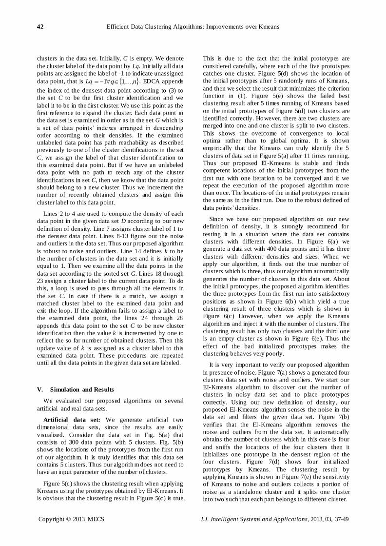
visualized. Consider the data set in Fig. 5(a) that
consists of 300 data points with 5 clusters. Fig. 5(b)
shows the locations of the prototypes from the first run
of our algorithm. It is truly identifies that this data set
contains 5 clusters. Thus our algorith m does not need to
have an input parameter of the number of clusters.
Figure 5(c) shows the clustering result when applying
Kmeans using the prototypes obtained by EI-Kmeans. It
is obvious that the clustering result in Figure 5(c) is true.
This is due to the fact that the initial prototypes are
considered carefully, where each of the five prototypes
catches one cluster. Figure 5(d) shows the location of
the initial prototypes after 5 randomly runs of Kmeans,
and then we select the result that minimizes the criterion
function in (1). Figure 5(e) shows the failed best
clustering result after 5 times running of Kmeans based
on the initial prototypes of Figure 5(d) two clusters are
identified correctly. However, there are two clusters are
merged into one and one cluster is split to two clusters.
This shows the overcome of convergence to local
optima rather than to global optima. It is shown
empirically that the Kmeans can truly identify the 5
clusters of data set in Figure 5(a) after 11 t imes running.
Thus our proposed EI-Kmeans is stable and finds
competent locations of the init ial prototypes from the
first run with one iterat ion to be converged and if we
repeat the execution of the proposed algorithm more
than once. The locations of the in itial p rototypes remain
the same as in the first run. Due to the robust defined of
data points’ densities.
Since we base our proposed algorithm on our new
definit ion of density, it is strongly recommend for
testing it in a situation where the data set contains
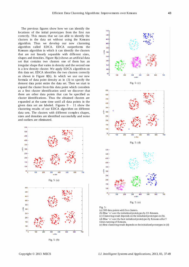
clusters with different densities. In Figure 6(a) we
generate a data set with 400 data points and it has three
clusters with different densities and sizes. When we
apply our algorithm, it finds out the true number of
clusters which is three, thus our algorithm automat ically
generates the number of clusters in this data set. About
the initial prototypes, the proposed algorithm identifies
the three prototypes from the first run into satisfactory
positions as shown in Figure 6(b) which yield a true
clustering result of three c lusters which is shown in
Figure 6(c) However, when we apply the Kmeans
algorithms and inject it with the number of clusters. The
clustering result has only two clusters and the third one
is an empty cluster as shown in Figure 6(e). Thus the
effect of the bad initialized prototypes makes the
clustering behaves very poorly.
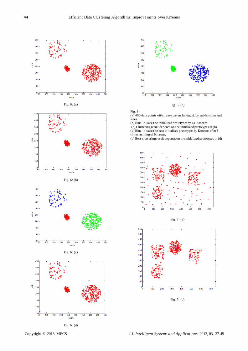
It is very important to verify our proposed algorithm
in presence of noise. Figure 7(a) shows a generated four
clusters data set with noise and outliers. We start our
EI-Kmeans algorithm to discover out the number of
clusters in noisy data set and to place prototypes
correctly. Using our new defin ition of density, our
proposed EI-Kmeans algorithm senses the noise in the
data set and filters the given data set. Figure 7(b)
verifies that the EI-Kmeans algorithm removes the
noise and outliers from the data set. It automatically
obtains the number of clusters which in this case is four
and sniffs the locations of the four clusters then it
init ializes one prototype in the densest region of the
four clusters. Figure 7(d) shows four init ialized
prototypes by Kmeans. The clustering result by
applying Kmeans is shown in Figure 7(e) the sensitivity
of Kmeans to noise and outliers collects a portion of
noise as a standalone cluster and it splits one cluster
into two such that each part belongs to different cluster.
Efficient Data Clustering Algorithms: Improvements over Kmeans 43
Copyright © 2013 MECS I.J. Intelligent Systems and Applications, 2013, 03, 37-49
The previous figures show how we can identify the
locations of the initial prototypes from the first run
correctly. Th is means that we can able to identify the
clusters in the data set without using the Kmeans
algorithm. Thus we develop our new clustering
algorithm called EDCA. EDCA outperforms the
Kmeans algorithm in which it can identify the clusters
that are not linearly separable with different sizes,
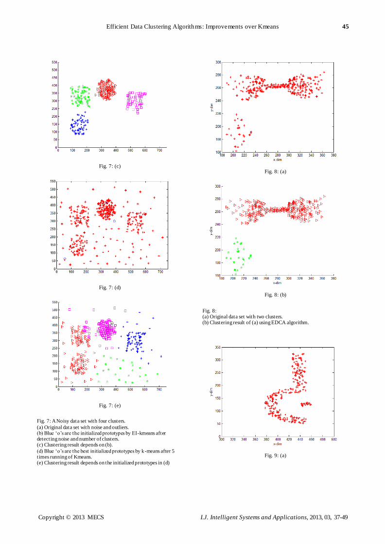
shapes and densities. Figure 8(a) shows an artificial data
set that contains two clusters one of them has an
irregular shape that varies in density and the second one
is a low density cluster. We apply EDCA a lgorithm on
this data set. EDCA identifies the two clusters correctly
as shown in Figure 8(b). In which we use our new
formula of data point density as in (3) to specify the
densest data point entire the data set. Then we start to
expand the cluster from this data point which considers
as a first cluster identification until we discover that
there are other data points that can be specified as
cluster identifications. Thus the obtained clusters are
expanded at the same time until all data points in the
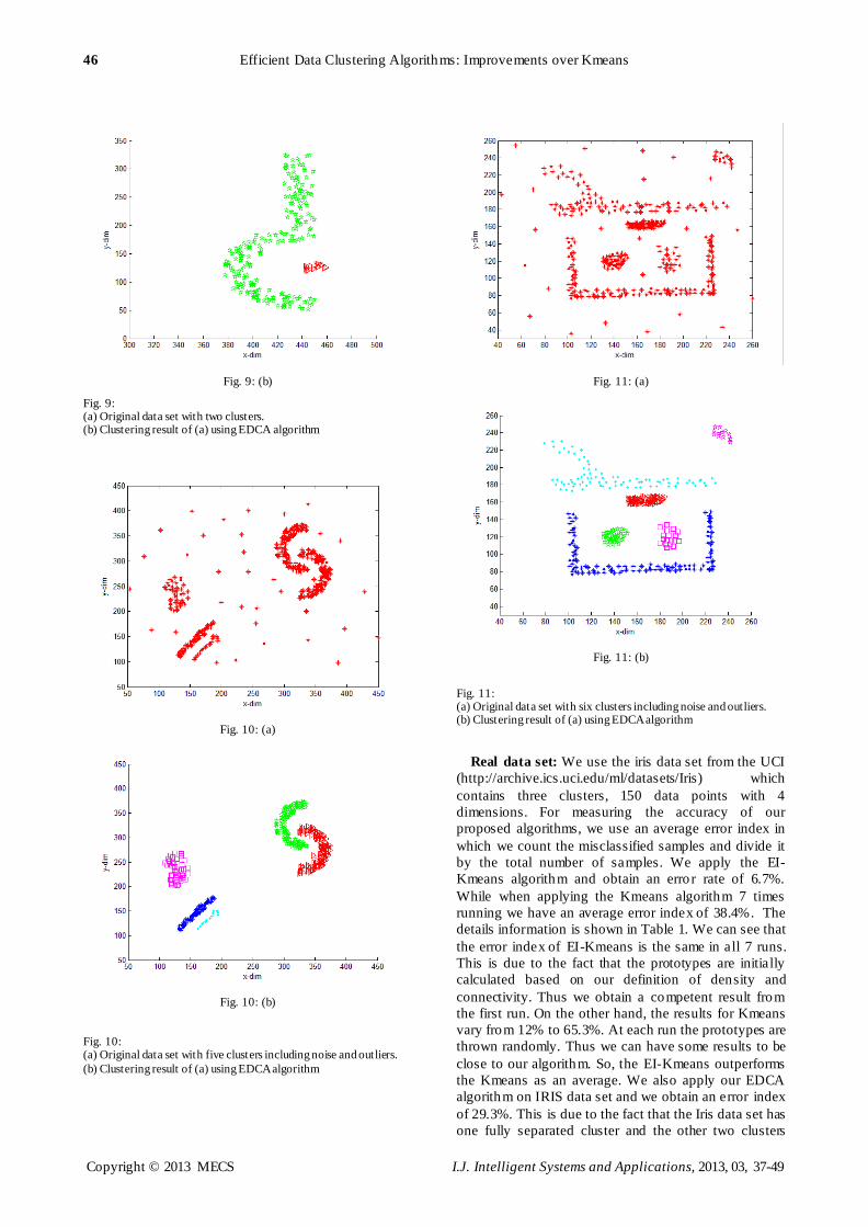
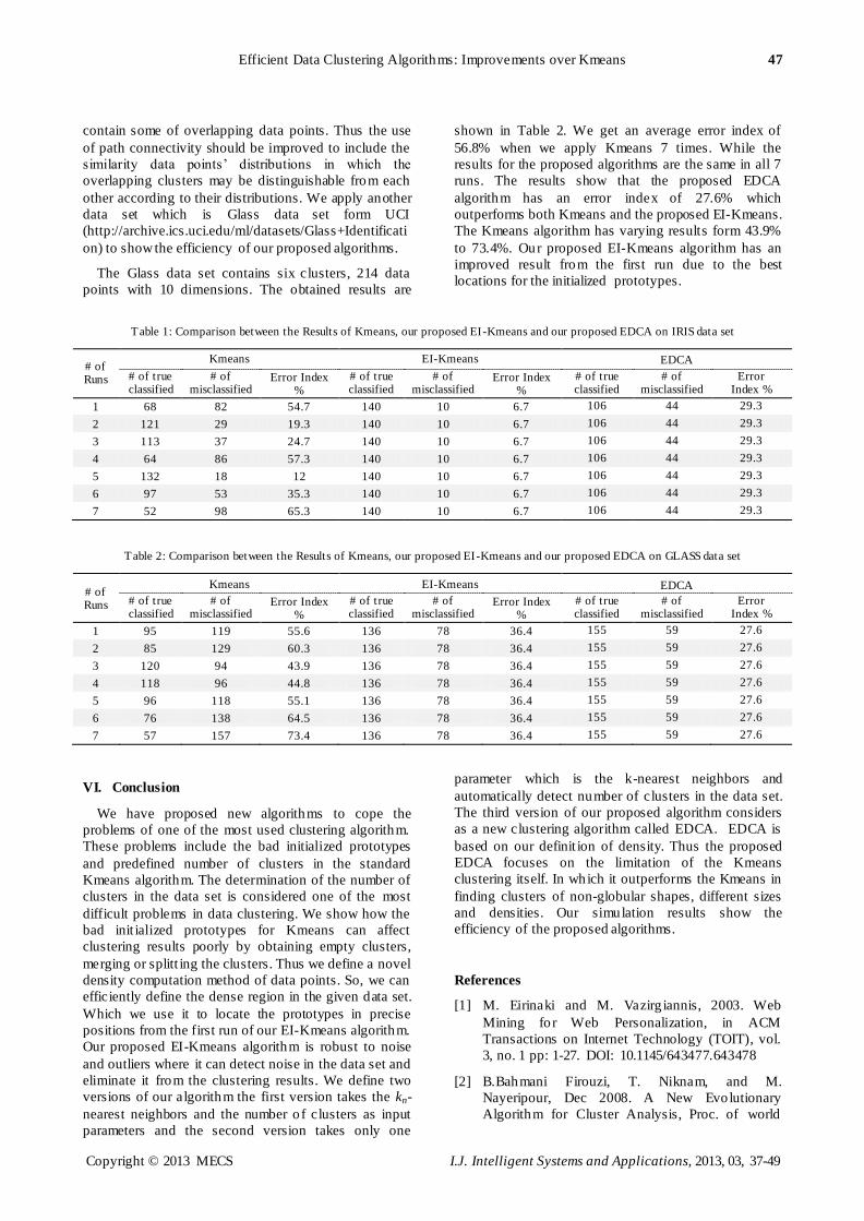
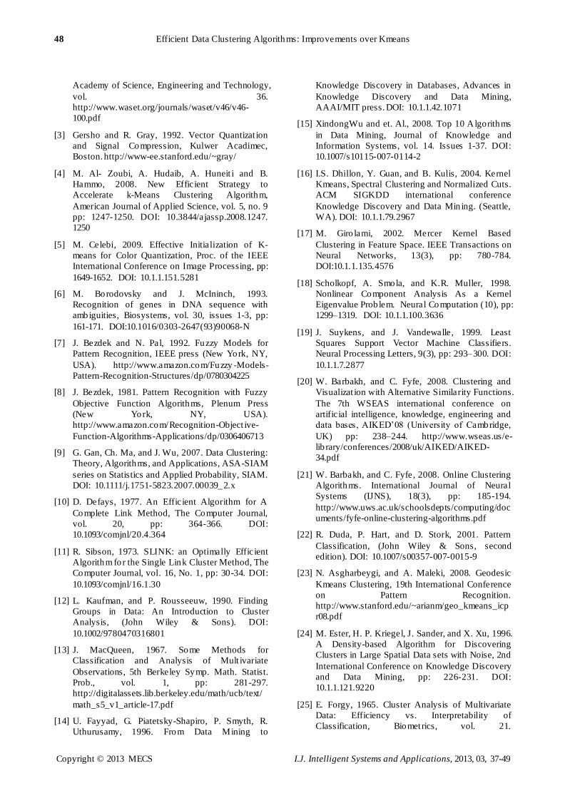
given data set are labeled. Figures 9 – 11 show the
clustering results of our EDCA algorithm on different
data sets. The clusters with d ifferent complex shapes,
sizes and densities are identified successfully and noise
and outliers are eliminated.
Fig. 5: (a)
Fig. 5: (b)
Fig. 5: (c)
Fig. 5: (d)
Fig. 5: (e)
Fig. 5: (a) 300 data points with five clusters. (b) Blue ‘o’s are the initialized prototypes by EI-Kmeans. (c) Clustering result depends on the initialized prototypes in (b).
(d) Blue ‘o’s are the best initialized prototypes by Kmeans after 5 t imes running of Kmeans. (e) Best clustering result depends on the initialized prototypes in (d)
44 Efficient Data Clustering Algorithms: Improvements over Kmeans
Copyright © 2013 MECS I.J. Intelligent Systems and Applications, 2013, 03, 37-49
Fig. 6: (a)
Fig. 6: (b)
Fig. 6: (c)
Fig. 6: (d)
Fig. 6: (e)
Fig. 6: (a) 400 data points with three clusters having different densities and sizes. (b) Blue ‘o’s are the initialized prototypes by EI-Kmeans.
(c) Clustering result depends on the initialized prototypes in (b). (d) Blue ‘o’s are the best initialized prototypes by Kmeans after 5 t imes running of Kmeans.
(e) Best clustering result depends on the initialized prototypes in (d)
Fig. 7: (a)
Fig. 7: (b)
Efficient Data Clustering Algorithms: Improvements over Kmeans 45
Copyright © 2013 MECS I.J. Intelligent Systems and Applications, 2013, 03, 37-49
Fig. 7: (c)
Fig. 7: (d)
Fig. 7: (e)
Fig. 7: A Noisy data set with four clusters.
(a) Original data set with noise and outliers. (b) Blue ‘o’s are the initialized prototypes by EI-kmeans after detecting noise and number of clusters. (c) Clustering result depends on (b).
(d) Blue ‘o’s are the best initialized prototypes by k-means after 5 times running of Kmeans. (e) Clustering result depends on the initialized prototypes in (d)
Fig. 8: (a)
Fig. 8: (b)
Fig. 8: (a) Original data set with two clusters. (b) Clustering result of (a) using EDCA algorithm.
Fig. 9: (a)
46 Efficient Data Clustering Algorithms: Improvements over Kmeans
Copyright © 2013 MECS I.J. Intelligent Systems and Applications, 2013, 03, 37-49
Fig. 9: (b)
Fig. 9: (a) Original data set with two clusters. (b) Clustering result of (a) using EDCA algorithm
Fig. 10: (a)
Fig. 10: (b)
Fig. 10: (a) Original data set with five clusters including noise and outliers.
(b) Clustering result of (a) using EDCA algorithm
Fig. 11: (a)
Fig. 11: (b)
Fig. 11: (a) Original data set with six clusters including noise and outliers. (b) Clustering result of (a) using EDCA algorithm
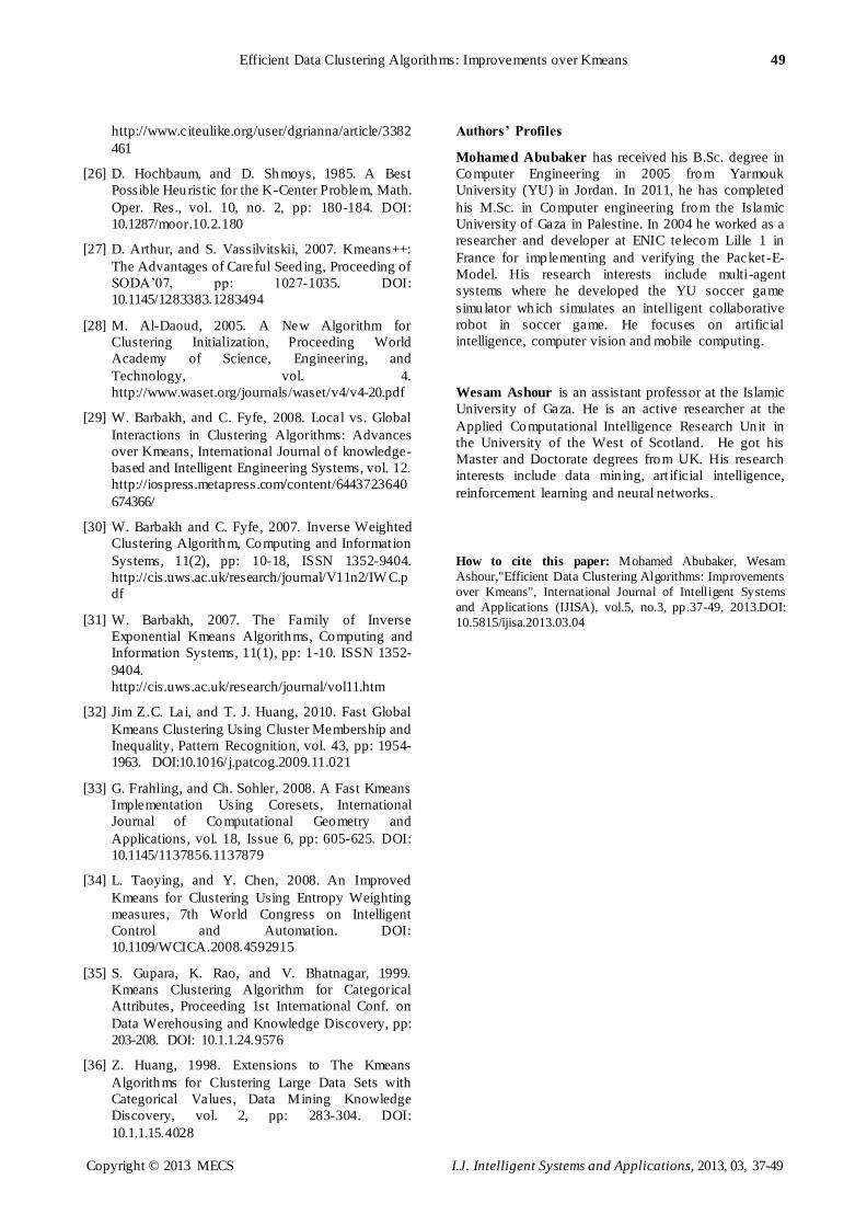
Real data set: We use the iris data set from the UCI
(http://archive.ics.uci.edu/ml/datasets/Iris) which
contains three clusters, 150 data points with 4
dimensions. For measuring the accuracy of our
proposed algorithms, we use an average error index in
which we count the misclassified samples and divide it
by the total number of samples. We apply the EI-
Kmeans algorithm and obtain an erro r rate of 6.7%.
While when applying the Kmeans algorithm 7 times
running we have an average error index of 38.4%. The
details information is shown in Table 1. We can see that
the error index of EI-Kmeans is the same in all 7 runs.
This is due to the fact that the prototypes are initially
calculated based on our definition of density and
connectivity. Thus we obtain a competent result from
the first run. On the other hand, the results for Kmeans
vary from 12% to 65.3%. At each run the prototypes are
thrown randomly. Thus we can have some results to be
close to our algorithm. So, the EI-Kmeans outperforms
the Kmeans as an average. We also apply our EDCA
algorithm on IRIS data set and we obtain an error index
of 29.3%. This is due to the fact that the Iris data set has
one fully separated cluster and the other two clusters
Efficient Data Clustering Algorithms: Improvements over Kmeans 47
Copyright © 2013 MECS I.J. Intelligent Systems and Applications, 2013, 03, 37-49
contain some of overlapping data points. Thus the use
of path connectivity should be improved to include the
similarity data points’ distributions in which the
overlapping clusters may be distinguishable from each
other according to their distributions. We apply another
data set which is Glass data set form UCI
(http://archive.ics.uci.edu/ml/datasets/Glass+Identificati
on) to show the efficiency of our proposed algorithms.
The Glass data set contains six clusters, 214 data
points with 10 dimensions. The obtained results are
shown in Table 2. We get an average error index of
56.8% when we apply Kmeans 7 times. While the
results for the proposed algorithms are the same in all 7
runs. The results show that the proposed EDCA
algorithm has an error index of 27.6% which
outperforms both Kmeans and the proposed EI-Kmeans.
The Kmeans algorithm has varying results form 43.9%
to 73.4%. Our proposed EI-Kmeans algorithm has an
improved result from the first run due to the best
locations for the initialized prototypes.
Table 1: Comparison between the Results of Kmeans, our proposed EI-Kmeans and our proposed EDCA on IRIS data set
# of Runs
Kmeans EI-Kmeans EDCA
# of true classified
# of misclassified
Error Index %
# of true classified
# of misclassified
Error Index %
# of true classified
# of misclassified
Error Index %
1 68 82 54.7 140 10 6.7 106 44 29.3
2 121 29 19.3 140 10 6.7 106 44 29.3
3 113 37 24.7 140 10 6.7 106 44 29.3
4 64 86 57.3 140 10 6.7 106 44 29.3
5 132 18 12 140 10 6.7 106 44 29.3
6 97 53 35.3 140 10 6.7 106 44 29.3
7 52 98 65.3 140 10 6.7 106 44 29.3
Table 2: Comparison between the Results of Kmeans, our proposed EI-Kmeans and our proposed EDCA on GLASS data set
# of Runs
Kmeans EI-Kmeans EDCA
# of true classified
# of misclassified
Error Index %
# of true classified
# of misclassified
Error Index %
# of true classified
# of misclassified
Error Index %
1 95 119 55.6 136 78 36.4 155 59 27.6
2 85 129 60.3 136 78 36.4 155 59 27.6
3 120 94 43.9 136 78 36.4 155 59 27.6
4 118 96 44.8 136 78 36.4 155 59 27.6
5 96 118 55.1 136 78 36.4 155 59 27.6
6 76 138 64.5 136 78 36.4 155 59 27.6
7 57 157 73.4 136 78 36.4 155 59 27.6
VI. Conclusion
We have proposed new algorithms to cope the
problems of one of the most used clustering algorithm.
These problems include the bad initialized prototypes
and predefined number of clusters in the standard
Kmeans algorithm. The determination of the number of
clusters in the data set is considered one of the most
difficult problems in data clustering. We show how the
bad init ialized prototypes for Kmeans can affect
clustering results poorly by obtaining empty clusters,
merging or splitt ing the clusters. Thus we define a novel
density computation method of data points. So, we can
efficiently define the dense region in the given data set.
Which we use it to locate the prototypes in precise
positions from the first run of our EI-Kmeans algorithm.
Our proposed EI-Kmeans algorithm is robust to noise
and outliers where it can detect noise in the data set and
eliminate it from the clustering results. We define two
versions of our algorithm the first version takes the kn-
nearest neighbors and the number o f clusters as input
parameters and the second version takes only one
parameter which is the k-nearest neighbors and
automatically detect number of clusters in the data set.
The third version of our proposed algorithm considers
as a new clustering algorithm called EDCA. EDCA is
based on our definit ion of density. Thus the proposed
EDCA focuses on the limitation of the Kmeans
clustering itself. In which it outperforms the Kmeans in
finding clusters of non-globular shapes, different sizes
and densities. Our simulation results show the
efficiency of the proposed algorithms.
References
[1] M. Eirinaki and M. Vazirg iannis, 2003. Web
Mining fo r Web Personalization, in ACM
Transactions on Internet Technology (TOIT), vol.
3, no. 1 pp: 1-27. DOI: 10.1145/643477.643478
[2] B.Bahmani Firouzi, T. Niknam, and M.
Nayeripour, Dec 2008. A New Evolutionary
Algorithm for Cluster Analysis, Proc. of world
48 Efficient Data Clustering Algorithms: Improvements over Kmeans
Copyright © 2013 MECS I.J. Intelligent Systems and Applications, 2013, 03, 37-49
Academy of Science, Engineering and Technology,
vol. 36.
http://www.waset.org/journals/waset/v46/v46-
100.pdf
[3] Gersho and R. Gray, 1992. Vector Quantizat ion
and Signal Compression, Kulwer Acadimec,
Boston. http://www-ee.stanford.edu/~gray/
[4] M. Al- Zoubi, A. Hudaib, A. Huneit i and B.
Hammo, 2008. New Efficient Strategy to
Accelerate k-Means Clustering Algorithm,
American Journal of Applied Science, vol. 5, no. 9
pp: 1247-1250. DOI: 10.3844/ajassp.2008.1247.
1250
[5] M. Celebi, 2009. Effective Initialization of K-
means for Color Quantization, Proc. of the IEEE
International Conference on Image Processing, pp:
1649-1652. DOI: 10.1.1.151.5281
[6] M. Borodovsky and J. McIninch, 1993.
Recognition of genes in DNA sequence with
ambiguities, Biosystems, vol. 30, issues 1-3, pp:
161-171. DOI:10.1016/0303-2647(93)90068-N
[7] J. Bezdek and N. Pal, 1992. Fuzzy Models for
Pattern Recognition, IEEE press (New York, NY,
USA). http://www.amazon.com/Fuzzy -Models-
Pattern-Recognition-Structures/dp/0780304225
[8] J. Bezdek, 1981. Pattern Recognition with Fuzzy
Objective Function Algorithms, Plenum Press
(New York, NY, USA).
http://www.amazon.com/Recognition-Object ive-
Function-Algorithms-Applications/dp/0306406713
[9] G. Gan, Ch. Ma, and J. Wu, 2007. Data Clustering:
Theory, Algorithms, and Applications, ASA-SIAM
series on Statistics and Applied Probability, SIAM.
DOI: 10.1111/j.1751-5823.2007.00039_2.x
[10] D. Defays, 1977. An Efficient Algorithm for A
Complete Link Method, The Computer Journal,
vol. 20, pp: 364-366. DOI:
10.1093/comjnl/20.4.364
[11] R. Sibson, 1973. SLINK: an Optimally Efficient
Algorithm for the Single Link Cluster Method, The
Computer Journal, vol. 16, No. 1, pp: 30-34. DOI:
10.1093/comjnl/16.1.30
[12] L. Kaufman, and P. Rousseeuw, 1990. Finding
Groups in Data: An Introduction to Cluster
Analysis, (John Wiley & Sons). DOI:
10.1002/9780470316801
[13] J. MacQueen, 1967. Some Methods for
Classification and Analysis of Mult ivariate
Observations, 5th Berkeley Symp. Math. Statist.
Prob., vol. 1, pp: 281-297.
http://digitalassets.lib.berkeley.edu/math/ucb/text/
math_s5_v1_article-17.pdf
[14] U. Fayyad, G. Piatetsky-Shapiro, P. Smyth, R.
Uthurusamy, 1996. From Data Mining to
Knowledge Discovery in Databases, Advances in
Knowledge Discovery and Data Mining,
AAAI/MIT press. DOI: 10.1.1.42.1071
[15] XindongWu and et. Al., 2008. Top 10 A lgorithms
in Data Mining, Journal of Knowledge and
Information Systems, vol. 14. Issues 1-37. DOI:
10.1007/s10115-007-0114-2
[16] I.S. Dhillon, Y. Guan, and B. Kulis, 2004. Kernel
Kmeans, Spectral Clustering and Normalized Cuts.
ACM SIGKDD international conference
Knowledge Discovery and Data Min ing. (Seattle,
WA). DOI: 10.1.1.79.2967
[17] M. Giro lami, 2002. Mercer Kernel Based
Clustering in Feature Space. IEEE Transactions on
Neural Networks, 13(3), pp: 780-784.
DOI:10.1.1.135.4576
[18] Scholkopf, A. Smola, and K.R. Muller, 1998.
Nonlinear Component Analysis As a Kernel
Eigenvalue Prob lem. Neural Computation (10), pp:
1299–1319. DOI: 10.1.1.100.3636
[19] J. Suykens, and J. Vandewalle, 1999. Least
Squares Support Vector Machine Classifiers.
Neural Processing Letters, 9(3), pp: 293–300. DOI:
10.1.1.7.2877
[20] W. Barbakh, and C. Fyfe, 2008. Clustering and
Visualizat ion with Alternative Similarity Functions.
The 7th WSEAS international conference on
artificial intelligence, knowledge, engineering and
data bases, AIKED’08 (University of Cambridge,
UK) pp: 238–244. http://www.wseas.us/e-
lib rary/conferences/2008/uk/AIKED/AIKED-
34.pdf
[21] W. Barbakh, and C. Fyfe, 2008. Online Clustering
Algorithms. International Journal of Neural
Systems (IJNS), 18(3), pp: 185-194.
http://www.uws.ac.uk/schoolsdepts/computing/doc
uments/fyfe-online-clustering-algorithms.pdf
[22] R. Duda, P. Hart, and D. Stork, 2001. Pattern
Classification, (John Wiley & Sons, second
edition). DOI: 10.1007/s00357-007-0015-9
[23] N. Asgharbeygi, and A. Maleki, 2008. Geodesic
Kmeans Clustering, 19th International Conference
on Pattern Recognition.
http://www.stanford.edu/~arianm/geo_kmeans_icp
r08.pdf
[24] M. Ester, H. P. Kriegel, J. Sander, and X. Xu, 1996.
A Density-based Algorithm for Discovering
Clusters in Large Spatial Data sets with Noise, 2nd
International Conference on Knowledge Discovery
and Data Mining, pp: 226-231. DOI:
10.1.1.121.9220
[25] E. Forgy, 1965. Cluster Analysis of Multivariate
Data: Efficiency vs. Interpretability of
Classification, Biometrics, vol. 21.
Efficient Data Clustering Algorithms: Improvements over Kmeans 49
Copyright © 2013 MECS I.J. Intelligent Systems and Applications, 2013, 03, 37-49
http://www.citeulike.org/user/dgrianna/article/3382
461
[26] D. Hochbaum, and D. Shmoys, 1985. A Best
Possible Heuristic for the K-Center Problem, Math.
Oper. Res., vol. 10, no. 2, pp: 180-184. DOI:
10.1287/moor.10.2.180
[27] D. Arthur, and S. Vassilvitskii, 2007. Kmeans++:
The Advantages of Care ful Seed ing, Proceeding of
SODA’07, pp: 1027-1035. DOI:
10.1145/1283383.1283494
[28] M. Al-Daoud, 2005. A New Algorithm for
Clustering Initialization, Proceeding World
Academy of Science, Engineering, and
Technology, vol. 4.
http://www.waset.org/journals/waset/v4/v4-20.pdf
[29] W. Barbakh, and C. Fyfe, 2008. Local vs. Global
Interactions in Clustering Algorithms: Advances
over Kmeans, International Journal o f knowledge-
based and Intelligent Engineering Systems, vol. 12.
http://iospress.metapress.com/content/6443723640
674366/
[30] W. Barbakh and C. Fyfe, 2007. Inverse Weighted
Clustering Algorithm, Computing and Informat ion
Systems, 11(2), pp: 10-18, ISSN 1352-9404.
http://cis.uws.ac.uk/research/journal/V11n2/IW C.p
df
[31] W. Barbakh, 2007. The Family of Inverse
Exponential Kmeans Algorithms, Computing and
Information Systems, 11(1), pp: 1-10. ISSN 1352-
9404.
http://cis.uws.ac.uk/research/journal/vol11.htm
[32] Jim Z.C. Lai, and T. J. Huang, 2010. Fast Global
Kmeans Clustering Using Cluster Membership and
Inequality, Pattern Recognition, vol. 43, pp: 1954-
1963. DOI:10.1016/ j.patcog.2009.11.021
[33] G. Frahling, and Ch. Sohler, 2008. A Fast Kmeans
Implementation Using Coresets, International
Journal of Computational Geometry and
Applications, vol. 18, Issue 6, pp: 605-625. DOI:
10.1145/1137856.1137879
[34] L. Taoying, and Y. Chen, 2008. An Improved
Kmeans for Clustering Using Entropy Weighting
measures, 7th World Congress on Intelligent
Control and Automation. DOI:
10.1109/WCICA.2008.4592915
[35] S. Gupara, K. Rao, and V. Bhatnagar, 1999.
Kmeans Clustering Algorithm for Categorical
Attributes, Proceeding 1st International Conf. on
Data Werehousing and Knowledge Discovery, pp:
203-208. DOI: 10.1.1.24.9576
[36] Z. Huang, 1998. Extensions to The Kmeans
Algorithms for Clustering Large Data Sets with
Categorical Values, Data Mining Knowledge
Discovery, vol. 2, pp: 283-304. DOI:
10.1.1.15.4028
Authors’ Profiles
Mohamed Abubaker has received his B.Sc. degree in
Computer Engineering in 2005 from Yarmouk
University (YU) in Jordan. In 2011, he has completed
his M.Sc. in Computer engineering from the Islamic
University of Gaza in Palestine. In 2004 he worked as a
researcher and developer at ENIC telecom Lille 1 in
France for implementing and verifying the Packet-E-
Model. His research interests include multi-agent
systems where he developed the YU soccer game
simulator which simulates an intelligent collaborative
robot in soccer game. He focuses on artificial
intelligence, computer vision and mobile computing.
Wesam Ashour is an assistant professor at the Islamic
University of Gaza. He is an active researcher at the
Applied Computational Intelligence Research Unit in
the University of the West of Scotland. He got his
Master and Doctorate degrees from UK. His research
interests include data min ing, art ificial intelligence,
reinforcement learning and neural networks.
How to cite this paper: Mohamed Abubaker, Wesam
Ashour,"Efficient Data Clustering Algorithms: Improvements
over Kmeans", International Journal of Intelligent Systems
and Applications (IJISA), vol.5, no.3, pp.37-49, 2013.DOI:
10.5815/ijisa.2013.03.04
Recommended