Efficient computation of acoustical scattering from N spheres via the
fast multipole method accelerated flexible generalized minimal residual method
Nail A. Gumerov Ramani Duraiswami
Institute for Advanced Computer StudiesUniversity of Maryland at College Park
www.umiacs.umd.edu/~gumerovwww.umiacs.umd.edu/~ramani
This study has been supported by NSF
OutlineIntroductionProblem FormulationMethod of Solution
Multipole Reexpansion (T-matrix) MethodIterative MethodsFast Multipole Method
Results of ComputationsConclusion

Introduction

Multiple Scattering ProblemsSound propagation in disperse media (particles, bubbles, etc.)Modeling of scattering from environment (humans, animals, fish, etc.)Electromagnetic scattering problems (microwaves, optics, etc.)Efficient parametrization in inverse problems (tomography, etc.)
Introduction
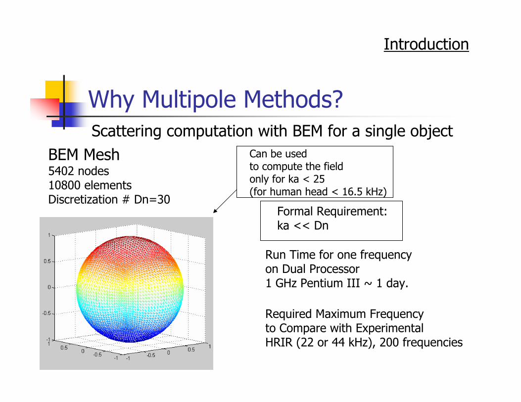
Why Multipole Methods?
Introduction
BEM Mesh5402 nodes10800 elementsDiscretization # Dn=30
Can be usedto compute the fieldonly for ka < 25 (for human head < 16.5 kHz)
Run Time for one frequencyon Dual Processor1 GHz Pentium III ~ 1 day.
Required Maximum Frequency to Compare with ExperimentalHRIR (22 or 44 kHz), 200 frequencies
Formal Requirement:ka << Dn
Scattering computation with BEM for a single object

Why Multipole Methods?
Meshless for spherical scatterersFast
Needs MeshRelatively Slow
Introduction
Multipole Methods BEM
Problem Formulation

Equations and Boundary Conditions
Helmholtz Equation
Impedance Boundary Conditions
Field Decomposition
Sommerfield Radiation Condition
4
2
1
6
5
3
Incident Wave
Formulation
Wave EquationFourierTransform

Multipole Reexpansion(T-Matrix) Method
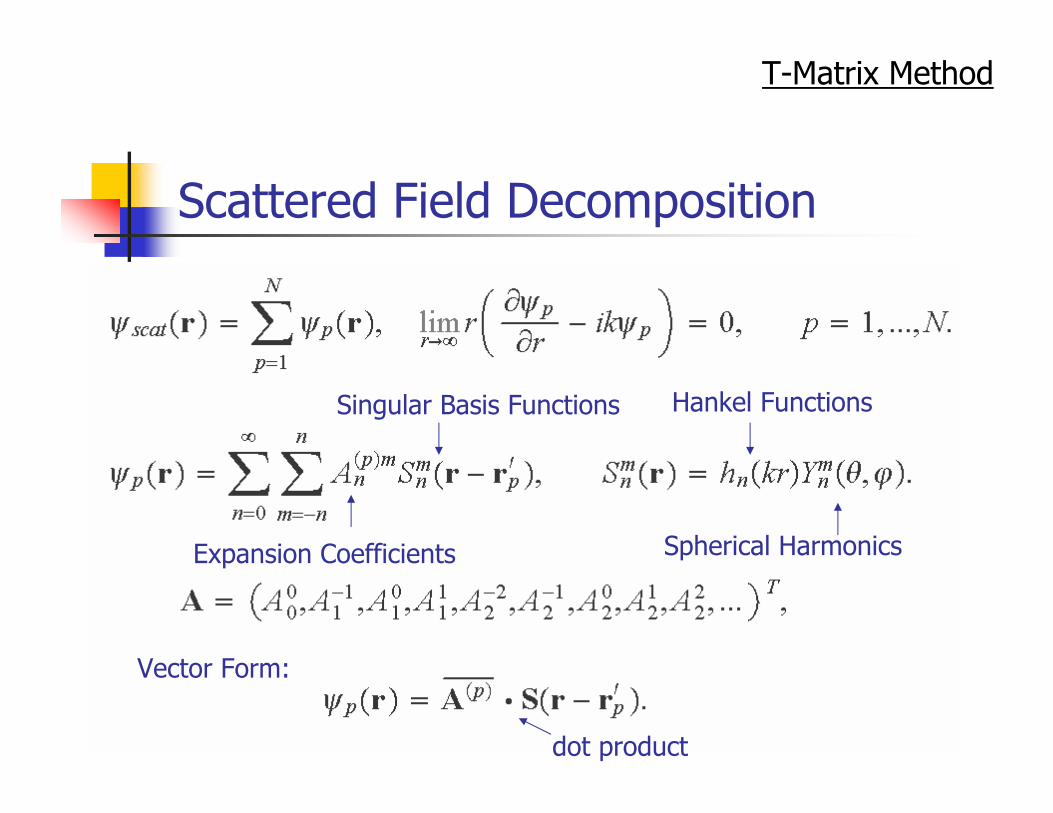
Scattered Field Decomposition
T-Matrix Method
Expansion Coefficients
Singular Basis Functions Hankel Functions
Spherical Harmonics
Vector Form:
dot product

Incident Field Decompositionand T-matrix for a Single Sphere
T-Matrix Method
Regular Basis Functions Bessel Functions
Analytical Solution of the Problem:
T-matrix

Solution of Multiple Scattering Problem
T-Matrix Method
4
2
1
6
53
Incident Wave
Scattered Wave
Coupled System of Equations:
(S|R)-TranslationMatrix
“Effective” Incident Field

Reexpansions/Translations
T-Matrix Method
q
p
M
O
rp
rq
r’pr’q
r’pq
r q
p
M
O
rp
rq
r’pr’q
r’pq
r

Two Spheres: Convergence with Respect to Truncation Number
T-matrix Method
-30
-20
-10
0
10
0 10 20 30 40 50Truncation Number
HR
TF (d
B)
ka1=30
5110
20
Two spheres,θ1 = 60o, φ1 = 0o,rmin/a1 = 2.3253.
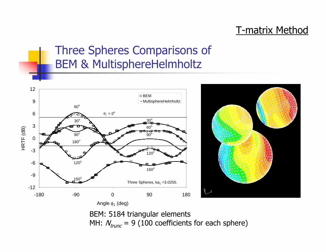
Three Spheres Comparisons ofBEM & MultisphereHelmholtz
T-matrix Method
BEM: 5184 triangular elementsMH: Ntrunc = 9 (100 coefficients for each sphere)
-12
-9
-6
-3
0
3
6
9
12
-180 -90 0 90 180
Angle φ1 (deg)
HR
TF (d
B)
BEMMultisphereHelmholtz
θ1 = 0o
30o
60o
90o
60o
30o
90o
120o
120o
150o
150o
180o
Three Spheres, ka1 =3.0255.

Conclusions on T-matrix MethodWe used recursive computation of translation matrices (Chew, 1992; Gumerov & Duraiswami, 2001). In some cases speed up of computations 103-104
times compared to BEM.But… Computational Complexity is O(N3P3)= O(N3
p6), where P= p2 is the total length of the vector of expansion coefficients. Method is not suitable for large N and ka.Details can be found in our paper JASA 112(6), 2002, 2688-2701.
T-matrix Method

Iterative Methods

Reflection MethodReflection (Simple Iteration) Method:
Iterative Methods

Convergence of Reflection Iteration Method
Iterative Methods
Exponential Convergence

Problems with the Reflection Technique
Large number of particlesLarge volume fractionsLarger ka

Krylov Subspace Method (GMRES)
Iterative Methods
Diagonal Matrix
The product of this matrix byAn arbitrary input vector can bedone fast with the FMM

FGMRES
Iterative Methods
LA = E LM-1(MA)=E
Unpreconditioned Right Preconditioner
1). Internal Loop:Solve M-1F=GRequires N(1)
iter multiplications MG2). External Loop:Requires N(2)
iter multiplications LG
Cost: C(1)·N(1)iter+ C·N(2)
iter
To converge requiresNiter multiplications LG,where G is an input vector
Cost: C·Niter
Substantial speed up if M≈L and C(1) « C

Multilevel Fast Multipole Method

Some Facts on the Fast Multipole Methods (FMM)
Introduced by Rokhlin & Greengard (1987,1988) for computation of 2D and 3D fields for Laplace Equation;Reduces complexity of matrix-vector product from O(N 2) to O(N) or O(NlogN) (depends on data structure);Hundreds of publications for various 1D, 2D, and 3D problems (Laplace, Helmholtz, Maxwell, Yukawa Potentials, etc.);Application to acoustical scattering problems (Koc & Chew, 1998; JASA);We developed modification of the FMM for solution of the Helmholtz equation: Level dependent truncation number + Fast translation operators based on rotation-coaxial translation decomposition.
MLFMM

Far and Near Fields
MLFMM
Neighborhood(Near Field)
Far Field

Computation of the Far Field (1)
MLFMM
xixc
(n,L)
y
1). Set Data Structure (hierarchically subdivide space with an oct-tree)
2). (S|S)-translate S-expansions for all scatterers in a box at the finest level to the center of the box and sum up (determine contribution to Far Field for each box at the finest level).
3). Recursively (S|S)-translate S-expansions to the center of the parent box and sum up (determine contribution to Far Field for each box at all courser levels).
UpwardPass
(From the finestto the coarsest
level)
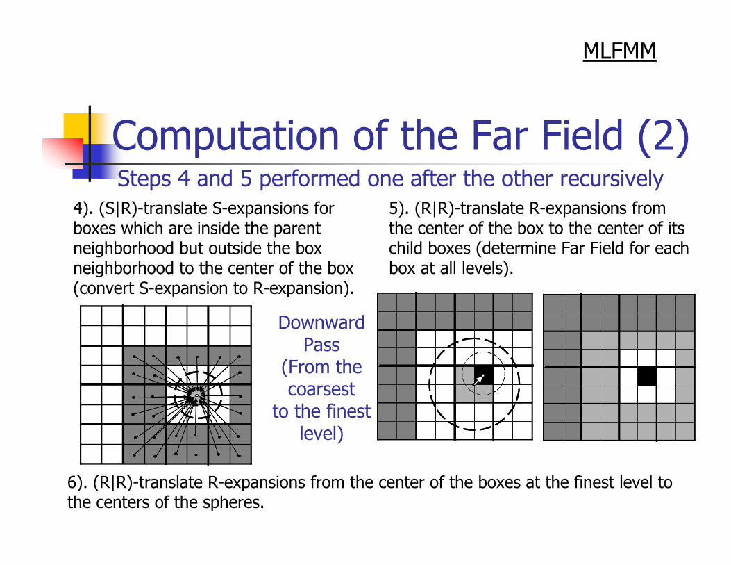
Computation of the Far Field (2)
MLFMM
4). (S|R)-translate S-expansions for boxes which are inside the parent neighborhood but outside the box neighborhood to the center of the box (convert S-expansion to R-expansion).
5). (R|R)-translate R-expansions from the center of the box to the center of its child boxes (determine Far Field for each box at all levels).
DownwardPass
(From the coarsest
to the finest level)
Steps 4 and 5 performed one after the other recursively
6). (R|R)-translate R-expansions from the center of the boxes at the finest level to the centers of the spheres.

Complexity of MLFMM
MLFMM
(For translation cost p3= P3/2 ):
(For each level of 3D space subdivision the computational work is approximately the same)

Computable Problems on Desktop PC
MLFMM
Met
hod
Number of Scatterers101 102 103100 104 105
BEM
Multipole Straightforward
Multipole Iterative
FMM
Also strongly depends on ka !

Preconditioned FGMRES
FGMRES

Results of Computations

Range of Parameters
Number of Spheres: 1-105;ka: 0.1-50;Random and regularly spaced grids of spheres;Polydispersity: 0.5-1.5 (ratio to the mean radius);Volume fractions: 0.01-0.25
Results

4 spheres (T-matrix straightforward)
Results
Vector of the incidentplane wave
Imaging plane
Scattererska=15.2
Incident Field Total Field Scattered Field

100 random spheres (MLFMM)
Results
ka = 1.6
Plane Wave Plane Wave
ka = 2.8ka = 1.6
Plane Wave Plane Wave
ka = 2.8
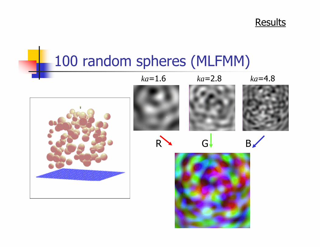
100 random spheres (MLFMM)
Results
ka=1.6 ka=4.8ka=2.8
R G B

1000 random spheres
ka=1
Results

10000 random spheres
ka = 0.75kD0 = 90
Results

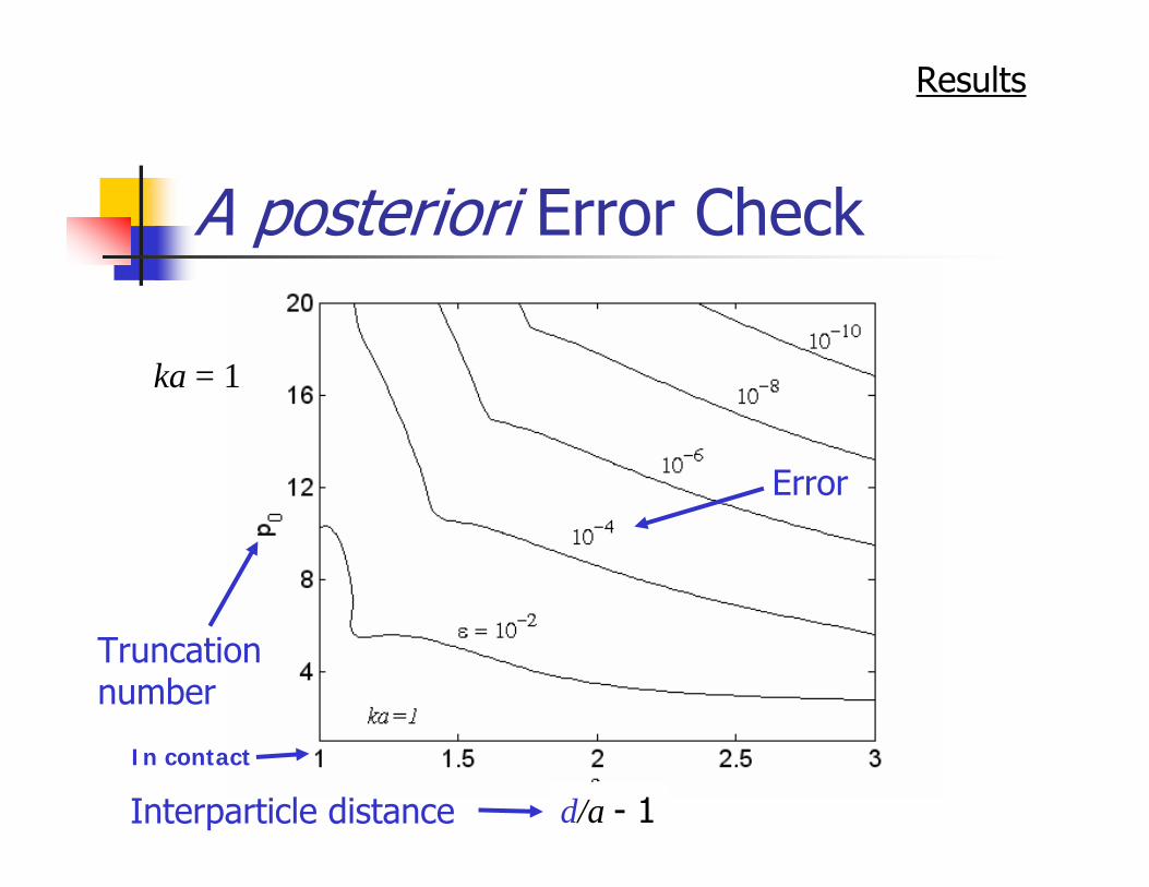
A posteriori Error Check
Results
A posteriori Error Check
Results
d/a - 1
ka = 1
Error
Truncation number
Interparticle distance
In contact
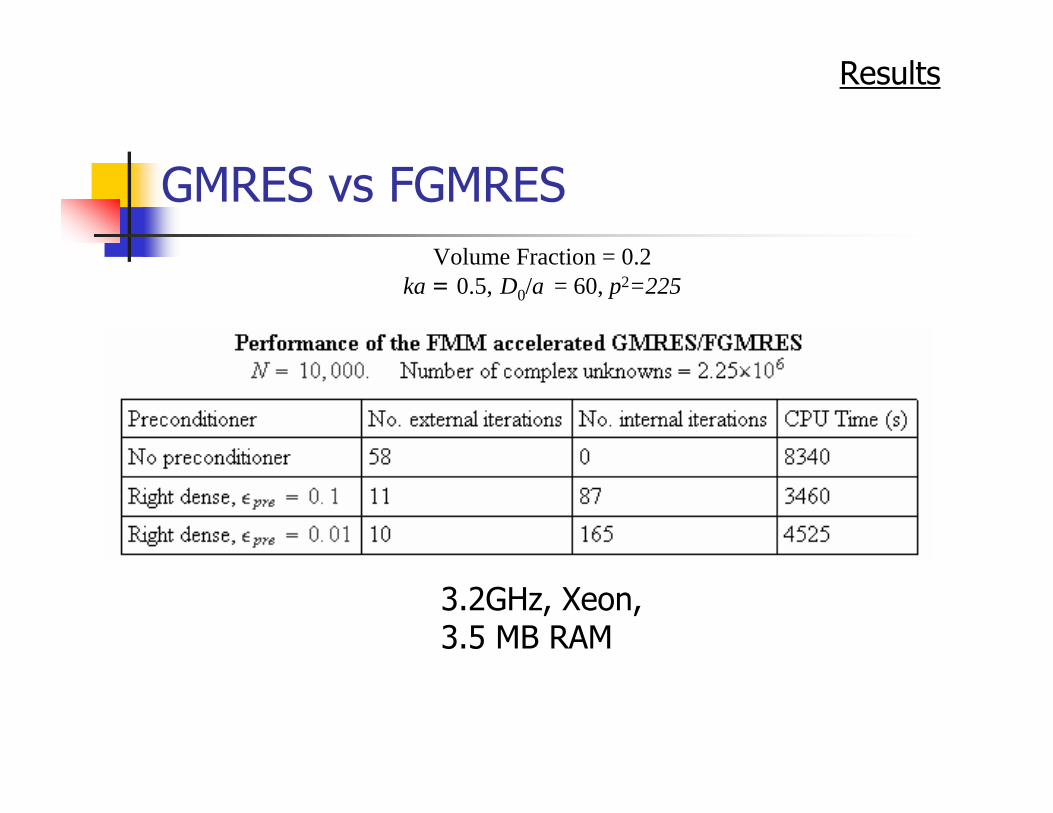
GMRES vs FGMRES
Results
Volume Fraction = 0.2ka = 0.5, D0/a = 60, p2=225
3.2GHz, Xeon,3.5 MB RAM
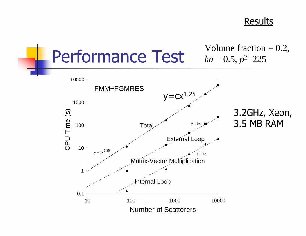
Performance Test
Results
0.1
1
10
100
1000
10000
10 100 1000 10000
Number of Scatterers
CP
U T
ime
(s)
Total
Matrix-Vector Multiplication
External Loop
Internal Loop
y = ax
y = bx
y = cx 1.25
FMM+FGMRESy=cx1.25
Volume fraction = 0.2,ka = 0.5, p2=225
3.2GHz, Xeon,3.5 MB RAM

Conclusions
We developed, implemented, and tested a T-matrix method for solution of multiple scattering problem accelerated by the Flexible GMRES and the FMM for the main system matrix and preconditioner multiplication. A modification of the FMM that uses level dependent truncation number and fast translation operators was developed. O(NlogN) complecxity of the method was proven theoretically and in the numerical tests.The convergence speed of the method depends on the volume fraction of scatterers, frequencies and the scatterer sizes. For dense systems the best performance was achieved using the right dense preconditioners which includes far field interactions.We performed study on the dependence of the error on the truncation numbers, which depend on the frequency, size and interparticle distances, and can be used for efficient error control.

Future work
Comparisons with continuum (averaging) theories and theories of wave propagation in random media;Computations of acoustic fields in disperse systems (bubbly liquids, particulate systems);Comparisons with experimental data.

THANK YOU !
Recommended