1
Efficiency of Banks in a Developing Economy: The Case of India
Dr Milind Sathye School of Accounting, Banking and Finance
University of Canberra Bruce ACT 2617
Tel: 61+2+6201 5489 Fax: 61+2+6201 5238
E-mail: [email protected]
Abstract
The objective of this paper is to measure the productive efficiency of banks in a
developing country, that is, India. The measurement of efficiency is done using Data
Envelopment Analysis (DEA). Two models have been constructed to show how
efficiency scores vary with change in inputs and outputs. The efficiency scores, for
three groups of banks, that is, publicly owned, privately owned and foreign owned,
are measured. The study shows that the mean efficiency score of Indian banks
compares well with the world mean efficiency score and the efficiency of private
sector commercial banks as a group is, paradoxically lower than that of public sector
banks and foreign banks in India. The study recommends that the existing policy of
reducing non-performing assets and rationalization of staff and branches may be
continued to obtain efficiency gains and make the Indian banks internationally
competitive which is a declared objective of the Government of India.
JEL classification: D61; G21; G34
Keywords: Bank efficiency; DEA analysis, Indian banks

2
Introduction
The objective of this study is to measure and to explain the measured variation in the
performance and therefore the productive efficiency of Indian commercial banks.
While many similar studies have evaluated the performance of banking sector in the
US and other developed countries, very few studies have evaluated the performance
of banking sectors in developing economies. Earlier though, Tyagarajan (1975),
Rangarajan and Mampilly (1972) and Subramanyam (1993) have examined various
issues relating to the performance of Indian banks, none of these studies have
examined the efficiency of bank service provision in India. Some recent studies did
measure the efficiency in service provision of Indian banks but they suffer from
certain limitations as indicated in this paper.
The main impetus for this study was the appointment of the (second) Narsimham
Committee (1997) by the Government of India, with a mandate to suggest a
programme of banking sector reforms so as to ‘strengthen India’s banking system and
make it internationally competitive’. This obviously requires that the relative
efficiency of Indian banks is measured and compared with banking efficiency in other
countries. Secondly, a scheme of voluntary redundancies for bank employees is under
consideration by the Indian Banks’ Association. In this context, the efficiency issues
of banks in India have again come to the fore. Thirdly, Indian banking is particularly
interesting because of the diversity of bank ownership forms. Indian banks can be
classified into three ownership groups; publicly owned, privately owned and foreign
owned. It is expected that there will be performance variation across groups of banks.
3
This study will quantify and explain the performance variation. Lastly, there is little
reliable empirical research on bank efficiency in India although Bhattacharya et al.
(1997), Chatterjee (1997) and Saha et al. (2000) have examined various issues relating
to the performance of Indian banks. This study measures relative efficiency of Indian
banks subsequent to the period used by the above studies. Additionally, it compares
the efficiency of Indian banks with that of the banks in other countries.
The paper has been organized as follows. A brief review of the current state of the
Indian banking sector is provided in section 2. In section 3 data and methodology are
discussed. Section 4 presents the results and section 5 concludes.
2. An overview of the Indian banking sector
It is important to take stock of the special features of the banking sector in India, in
order to put the efficiency issues in perspective. India is the largest country in South
Asia with a huge financial system characterized by many and varied financial
institutions and instruments. Indian banking sector was well developed even prior to
its political independence in 1947. ‘There was significant presence of both foreign
and domestic banks and well developed stock market’ (Bery, 1996, p. 245). The
system expanded rapidly after nationalization of major commercial banks in late 1969
and ‘now ranks in the top quarter among developing countries’ (Khanna, 1995, p.
265).

4
Table 1 below presents important banking indicators of commercial banks in India as
at the end of June 1998.
Table 1: Banking data commercial banks in India as of June 1998
Number Branches Deposits
(Rs. Billion)
Advances
(Rs. Billion)
Public Sector Banks 27 45,293 5,317 2,599
Private Sector Banks 34 4,664 695 354
Foreign Banks 42 182 429 292
Source: Indian Bank’s Association
Besides the above, as at the end of June 1998, there were 196 Regional Rural Banks
with 14,517 branches, 28 State Cooperative banks with 651 branches, 351 District
Central Cooperative Banks with 10,775 branches, 88,341 Primary Agricultural
Cooperative Credit Societies, 20 State Agricultural and Rural Development Banks
with 1,488 branches, and 706 Primary Land Development Banks with 646 branches
(Sathye, 1997). There also are several Urban Cooperative Banks and 22,000 non-bank
financial institutions (Khanna, 1995, p. 294).
At the top of the banking system is the Reserve Bank of India, which is responsible
for prudential supervision of banks, non-banks and for performing other central
banking functions. There were two successive nationalization’s of banks in India, one
in 1969 and the other in 1980 and as a result public sector banks occupy a
predominant role in Indian financial system. Despite a phenomenal expansion of
number of branches, the population served per branch stood at 13,000 (RTPB, 1996,
5
p. 126). This is due to the fact that population of the country has been growing
unabated (crossed 1 billion mark recently) and branch network cannot keep pace with
it due to the costs involved. In the year 1997-98, the aggregate deposits of the public
sector banks were of the order of Rs. 5,317 billion (51 per cent of GDP), that of
private sector commercial banks were Rs. 695 billion (7 percent of GDP) and foreign
banks were Rs. 429 billion (4 per cent of GDP). The advances were Rs. 2599 billion
(25 percent of GDP), Rs. 354 billion (3 percent of GDP), and Rs. 292 billion (3
percent of GDP) respectively. The public sector banks control over 80 percent of
banking business. The banking system has developed well over the years in terms of
its geographical coverage, deposit mobilization and credit expansion. With regard to
technology, it is underdeveloped. Foreign banks have started a few ATMs in
metropolitan centers in recent years.
Indian banking was subjected to tighter governmental control over the ownership
from the late 1960s known as social control over banks: the government nationalized
the banks later. The banks were subjected to directed credit, prescribed interest rates
and substantial pre-emption of deposits. The banking services that were mostly
confined to metropolitan areas were expanded to the rural areas. Thus, while at the
end of 1964 only 10 per cent of the commercial banks were located in rural areas, the
proportion increased to 45 per cent thirty years later. The share of advances to
activities in the priority sector1 increased substantially after nationalization. The
overall priority sector credit target is presently 40 per cent of net bank credit for both
public sector and private sector banks. For foreign banks, the target is 32 per cent. The
1 Priority sector refers to the lending for agriculture and other rural sector of the economy, poverty alleviation programmes, exports, small-scale industries and such other purposes.
6
share of priority sector advances in total credit of commercial banks increased from
14 per cent in 1969 to 30 per cent in 1980 and to 39 per cent in 1985 (Thakur, 1990).
Since the early 1990s, the Government of India has implemented many banking sector
reforms. These include lowering of the cash reserve ratio from 15 per cent (1993-94)
to present 8.5 percent (July 2000), lowering of the statutory liquidity ratio from 38.5
per cent (1992-93) to 28.2 per cent (1995-96), a gradual deregulation of interest rates
on deposits and lending, introduction of prudential norms in line with the international
standards and the like. A system of flexible exchange rates on current account has
been adopted. The Committee on the Financial System, appointed by the Government
of India in 1991, identified directed investment and credit programs as the two main
sources of declining efficiency, productivity and profitability among commercial
banks. Consequently, the percentage of priority sector advances has declined to 37 per
cent (1998) and percentage of rural branches network has come down to 42 per cent.
These and similar other policy initiatives indicate the desire to make Indian banking
more competitive by establishing a level playing field among the three groups of
banks. As more than eight years have now elapsed since the initiation of the banking
sector reforms, it is appropriate to take stock of the production efficiency of banks in
India.
3. Methodology
It is usual to measure the performance of banks using financial ratios. Yeh (1996)
notes that the major demerit of this approach is its reliance on benchmark ratios.
These benchmarks could be arbitrary and may mislead an analyst. Further, Sherman

7
and Gold (1985) note that financial ratios don’t capture the long-term performance,
and aggregate many aspects of performance such as operations, marketing and
financing. In recent years, there is a trend towards measuring bank performance using
one of the frontier analysis methods. In frontier analysis, the institutions that perform
better relative to a particular standard are separated from those that perform poorly.
Such separation is done either by applying a non-parametric or parametric frontier
analysis to firms within the financial services industry. The parametric approach
includes stochastic frontier analysis, the free disposal hull, thick frontier and the
Distribution Free Approaches (DFA), while the non-parametric approach is Data
Envelopment Analysis (DEA) (Molyneux et al. 1996). In this paper, the DEA
approach has been used. This approach has been used since “recent research has
suggested that the kind of mathematical programming procedure used by DEA for
efficient frontier estimation is comparatively robust” (Seiford and Thrall, 1990).
Furthermore, after Charnes, Cooper and Rhodes (1978) who coined the term DEA, a
‘large number of papers have extended and applied the DEA methodology’ (Coelli,
1996).
The present study uses the latest available published data for the year 1997-98
compiled by the Indian Banks’ Association (IBA, 1999). As per this database, in the
year 1997-98, there were 27 public sector commercial banks, 34 private sector
commercial banks and 42 foreign banks. Of these 103 banks, the data on some of the
inputs and outputs of nine banks (1 private sector and 8 foreign) were not available.
Hence these banks were excluded from the sample. The final sample thus had 27
public sector commercial banks, 33 private sector commercial banks and 34 foreign
banks. Thus, the total observations consisted of 94 banks.
8
The first step in the analysis is the measurement of bank performance. Following
Bhattacharya et al. (1997), performance has been associated with technical efficiency
(hereafter refereed to as ‘efficiency’). It is the ability to transform multiple resources
into multiple financial services. The efficiency has been calculated using variable
returns to scale (VRS) input oriented model of the DEA methodology. To measure
efficiency as directly as possible, that is, management’s success in controlling costs
and generating revenues (that is, x-efficiencies), two input and two output variables,
namely, interest expenses, non-interest expenses (inputs) and net interest income and
non-interest income (outputs) have been used (hereafter refereed to as Model A). A
second DEA analysis was run with deposits and staff numbers as inputs and net loans
and non-interest income as outputs (hereafter refereed to as Model B). In the Model
B, where a less direct approach is taken to measure efficiency, deposits replace
interest expense, staff numbers replace non-interest expenses and net loans become
proxy for net interest income. The two models have been used to show how
efficiency scores differ when inputs and outputs are changed.
The choice of inputs and outputs in DEA is a matter of long standing debate among
researchers. Two approaches exist. One is called the production approach while the
other an intermediation approach. The production approach uses number of accounts
of deposits or loans as inputs and outputs respectively. This approach assumes that
banks produce loans and other financial services. The intermediation approach on the
other hand considers banks as financial intermediaries and uses volume of deposits,
loans and other variables as inputs and outputs. Most of the DEA studies follow an
intermediation approach. Within the intermediation approach, the exact set of inputs
and outputs used depends largely on data availability. As already stated DEA is

9
sensitive to the choice of input-output variables. This is strength of the technique,
since it reveals which of the input-output variables need to be closely monitored by
bank management to improve efficiency. Avkiran (1999) has attempted a similar two-
model analysis for Australian banks.
Data Envelopment Analysis
DEA is a linear programming technique initially developed by Charnes, Cooper and
Rhodes (1978) to evaluate the efficiency of public sector non-profit organisations.
Sherman and Gold (1985) were the first to apply DEA to banking. DEA calculates the
relative efficiency scores of various Decision-Making Units (DMUs) in the particular
sample. The DMUs could be banks or branches of banks. The DEA measure
compares each of the banks/branches in that sample with the best practice in the
sample. It tells the user which of the DMUs in the sample are efficient and which are
not. The ability of the DEA to identify possible peers or role models as well as simple
efficiency scores gives it an edge over other methods. As an efficient frontier
technique, DEA identifies the inefficiency in a particular DMU by comparing it to
similar DMUs regarded as efficient, rather than trying to associate a DMU’s
performance with statistical averages that may not be applicable to that DMU.
DEA modelling allows the analyst to select inputs and outputs in accordance with a
managerial focus. This is an advantage of DEA since it opens the door to what-if
analysis. Furthermore, the technique works with variables of different units without
the need for standardisation (e.g. dollars, number of transactions, or number of staff).
Fried and Lovell (1994) have given a list of questions that DEA can help to answer.
10
However, DEA has some limitations. When the integrity of data has been violated,
DEA results cannot be interpreted with confidence. Another caveat of DEA is that
those DMUs indicated as efficient are only efficient in relation to others in the
sample. It may be possible for a unit outside the sample to achieve a higher efficiency
than the best practice DMU in the sample. Knowing which efficient banks are most
comparable to the inefficient bank enables the analyst to develop an understanding of
the nature of inefficiencies and re-allocate scarce resources to improve productivity.
This feature of DEA is clearly a useful decision-making tool in benchmarking. As a
matter of sound managerial practice, profitability measures should be compared with
DEA results and significant disagreements investigated. The DEA technique has been
used in efficiency analysis of banks (rather than branches); some recent examples are
Yue (1992), Berg et al.. (1993), Favero and Papi (1995), Wheelock and Wilson
(1995), Miller and Noulas (1996), Resti (1997) and Sathye (2001)2.
4. Results
The efficiency scores of each of the banks included in the sample are shown in
Appendix 1. In Table 2, some descriptive statistics about the banks in the sample has
been presented.
2 Readers interested in the details of the various frontier measurement techniques are encouraged to consult the works of Banker, Charnes, Cooper, Swarts and Thomas (1989), Bauer (1990), and Seiford and Thrall (1990), Aly and Seiford (1993) etc. There are a number of software options for running DEA. This study uses the software (DEAP) developed by Coelli (1996) to calculate the efficiency scores.
11
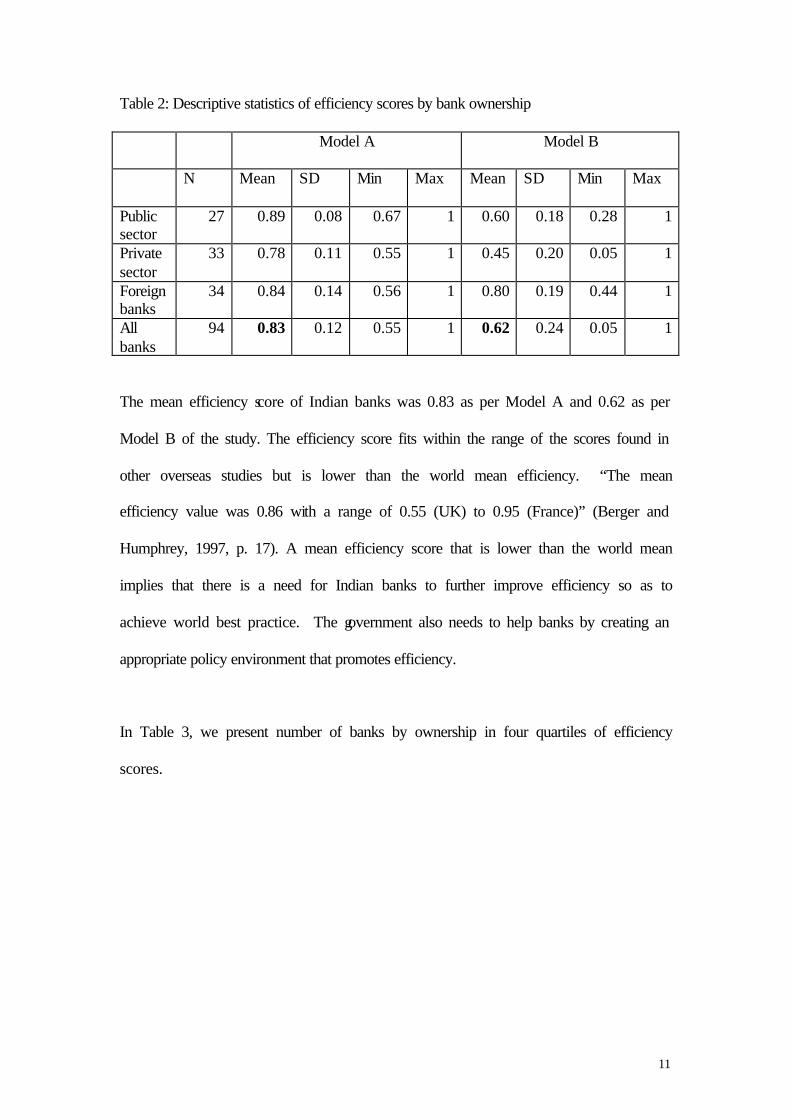
Table 2: Descriptive statistics of efficiency scores by bank ownership
Model A Model B
N Mean SD Min Max Mean SD Min Max
Public sector
27 0.89 0.08 0.67 1 0.60 0.18 0.28 1
Private sector
33 0.78 0.11 0.55 1 0.45 0.20 0.05 1
Foreign banks
34 0.84 0.14 0.56 1 0.80 0.19 0.44 1
All banks
94 0.83 0.12 0.55 1 0.62 0.24 0.05 1
The mean efficiency score of Indian banks was 0.83 as per Model A and 0.62 as per
Model B of the study. The efficiency score fits within the range of the scores found in
other overseas studies but is lower than the world mean efficiency. “The mean
efficiency value was 0.86 with a range of 0.55 (UK) to 0.95 (France)” (Berger and
Humphrey, 1997, p. 17). A mean efficiency score that is lower than the world mean
implies that there is a need for Indian banks to further improve efficiency so as to
achieve world best practice. The government also needs to help banks by creating an
appropriate policy environment that promotes efficiency.
In Table 3, we present number of banks by ownership in four quartiles of efficiency
scores.

12
Table 3: Number of banks in four quartiles of efficiency scores by bank ownership
Model A Model B
Public Private Foreign Total Public Private Foreign Total
Lowest efficiency (Q1) 1 12 10 23 5 15 3 23
Next to lowest quartile (Q2) 7 13 4 24 10 12 2 24
Next to Highest efficiency
quartile (Q3)
10 5 9 24 9 4 11 24
Highest efficiency quartile
(Q4)
9 3 11 23 3 2 18 23
Total 27 33 34 94 27 33 34 94
Banks on the Frontier
(efficiency score = 1)
4 1 10 15 3 1 12 16
The above table shows that as per Model A, of the 15 banks on the frontier, 10 were
foreign banks while as per Model B, out of the 16 banks on the frontier 12 were
foreign banks. Further, it could be seen that as per Model A, out of the 23 banks in
the highest efficiency quartile (Q4), 11 (48%) are foreign banks. As per Model B, out
of 23 banks 18 (78%) are in the Q4. This means that as a group more foreign banks
are in the highest efficiency quartile than public or private sector banks. Their
preponderance in Model B is, particularly, noteworthy. It shows that foreign banks
are much more efficient as a group in use of inputs of staff and deposits as compared
to public or private sector banks. As a group, the private sector commercial banks
have displayed lower efficiency level in both the models.
The banks that were on the efficiency frontier under both models included State Bank
of India, Bank of Baroda (two public sector banks), IndusInd bank (one private
sector) and Citi Bank, Bank of America, Deutsche Bank, Bank of Mauritius, Cho
13
Hung Bank, Sonali Bank and Arab Bank (seven foreign banks). The minimum
efficiency score in Model B for private sector bank was 0.05. This was because two
banks, Bank of Nainital and Bareilly Bank had scores of 0.05 and 0.06 respectively.
These outlier cases are because of peculiarity of the region in which these banks
operate. They are flush with deposits but have few avenues for lending. These banks
invest funds in government securities (which is not considered here as output due to
non-availability of data) hence these banks show low efficiency scores.
The scores computed using Model A and Model B need some explanation. As
already stated DEA is a flexible technique and produces efficiency scores that are
different when alternative sets of inputs and outputs are used. In Model A, we have
used prices of inputs (interest and non-interest expenses) as the input variables while
in Model B, mainly quantities of inputs (deposits and staff numbers) have been used
as input variables. Foreign banks as a group appear to be more efficient users of input
quantities to produce a given output as compared to the public sector banks and
private sector banks. This means that there are inefficiencies in use of these two
inputs (deposits and staff numbers) among the public sector and private sector banks
which these banks need to remedy to achieve increased efficiency. On the other hand,
foreign banks need to focus on pricing aspects (interest and non-interest income and
expenses) of their inputs and outputs to achieve higher efficiencies. The lower scores
for private sector banks in both the models could be because these banks are in the
expansion phase and could have higher amount of fixed assets employed which have
yet to start generating return.
The efficiency estimates as per this study compare well with the score estimated by
Bhattacharya et al. (1997). In their study the efficiency scores ranged from 79.19 to
14
80.44 in the years 1986 through 1991. In the study of Saha et al. (2000) where
efficiency scores have been estimated only for 25 public sector banks the estimates
ranged from 0.58 to 0.74 in the year 1995 and the mean score was 0.69. The inputs
and outputs, number of firms in the sample and the year are different in the present
study compared to these two studies. Bhattacharya et al. analyse data for the pre-
deregulation years while this study does so after sufficient period has elapsed since
deregulation. The banks have taken steps to lower the ratio of non-performing assets,
which has been brought down from 24 per cent in 1993-94 to 20 per cent in 1994-95
(Rangarajan, 1995). This would have helped in increasing interest income an input in
Model A. The banks need to continue their efforts to reduce the percentage of non-
performing assets to improve efficiency. Another important reason affecting the
efficiency of public sector banks, in particular, is the high establishment expenses as a
percentage of total expenses. In the year 1997-98, the ratio was 20.13 for public
sector banks, 9.87 for private sector commercial banks and 7.66 for foreign banks.
The public sector banks have recently introduced a voluntary redundancy scheme for
staff, which if successful will help bring down this ratio and thus improve efficiency
scores further.
5. Conclusion
Using published data, this paper worked out the production efficiency score of Indian
banks for the year 1997-98. The scores were calculated using the non-parametric
technique of Data Envelopment Analysis. The study shows that as per Model A, the
public sector banks have a higher mean efficiency score as compared to the private
sector and foreign commercial banks in India. As per Model B, they have lower mean

15
efficiency score than the foreign banks but still higher than private sector commercial
banks. Most banks on the frontier are foreign owned. The study recommends that the
existing policy of bringing down non-performing assets as well as curtailing the
establishment expenditure through voluntary retirement scheme for bank staff and
rationalization of rural branches are steps in the right direction that could help Indian
banks improve efficiency over a period of time so as to achieve world best practice.

16
References
Aly, A. I., Seiford, L. M. 1993. The mathematical programming approach to
efficiency analysis in: Fried, H. O., Lovell, C. A. K., Schmidt, S. S., (Eds) The
measurement of Productive Efficiency; Techniques and Applications, Oxford
University Press, U K, 120-159.
Avkiran, N. K. 1999. The evidence of efficiency gains: The role of mergers and the
benefits to the public. Journal of Banking and Finance 23, 991-1013.
Banker, R. D., Charnes, A., Cooper, W. W., Swarts, J., Thomas, D. A. 1989. An
introduction to Data Envelopment Analysis with some of its models and their uses, in
Chan, J. L., Patton J. M. (Eds.) Research in Governmental and Non Profit
Aaccounting, Vol. 5. Jai Press, Greenwich CN, 125-63.
Bauer, P. W. 1990. Recent developments in the econometric estimation of frontiers.
Journal of Econometrics 46, 39-56.
Berg, S. A. Forsund, F. R., Hjalmarsson, L. and Souminen, M. 1993. “Banking
efficiency in Nordic countries”, Journal of Banking and Finance, Vol. 17, 371-88.
Berger, A. N., Humphrey, D.B. 1997. “Efficiency of financial institutions:
International survey and directions for future research”, European Journal of
Operations Research (Special Issue) http://papers.ssrn.com/paper.taf?
ABSTRACT_ID=2140
17
Bery, S. 1996. “India: Commercial Bank Reform” in Financial Sector Reforms,
Economic Growth and Stability: Experiences in Selected Asian and Latin American
Countries (Ed) Faruqi, Shakil. EDI Seminar Series, The World Bank, Washington, D.
C.
Bhattacharya, A., Lovell, C.A.K., and Sahay, P. 1997. “The impact of liberalization
on the productive efficiency of Indian commercial banks”, European Journal of
Operational Research, 98, 332-345.
Charnes, A., Cooper, W.W., Rhodes, E. 1978. Measuring efficiency of decision
making units. European Journal of Operations Research 2, 429-44.
Chatterjee, G. 1997. “ Scale Economies in Banking: Indian Experience in Deregulated
Era”, RBI Occasional Papers, Vol. 18 No. 1, 25-59.
Coelli, T. 1996. A Guide to DEAP Version 2.1, A Data Envelopment Analysis
(Computer) Program. CEPA Working Paper 96/08.
Favero, C. A. and Papi, L. 1995. “Technical efficiency and scale efficiency in the
Italian banking sector: a non-parametric approach”m, Applied Economics, Vol. 27
No. 4, 385-95.

18
Fried, H. O., Lovell, C. A. K. 1994. Measuring efficiency and evaluating
performance. quoted in Data Envelopment Analysis: A technique for measuring the
efficiency of government service delivery. Steering Committee for the Review of
Commonwealth/state Service Provision. 1997. AGPS, Canberra.
IBA (Indian Banks’ Association). 1999. Performance Highlights of Banks 1997-98,
Indian Banks Association, Mumbai.
Khanna A. 1995. ‘South Asian Financial Sector Development’ in Financial Sector
Development in Asia, (Ed.) S. N. Zahid, Oxford University Press, Oxford.
Mester, L. J. 1996. “ A study of bank efficiency taking into account risk preferences”,
Journal of Banking and Finance, Vol.20 No. 6, 1025-45.
Miller, S. M. and Noulas, A. G. 1996. “The technical efficiency of large bank
production”, Journal of Banking and Finance, Vol. 20 No. 3, 495-509.
Molyneux, P., Altunbas, Y., Gardener, E. 1996. Efficiency in European Banking.
John Wiley Chichester 198.
Rangarajan, C. 1995. ‘Inaugural address at the 18th Bank Economists’ conference’,
Reserve Bank of India Bulletin, December, XLIX (12), Reserve Bank of India,
Mumbai.

19
Rangarajan, C., and Mampilly, P. 1972. “Economies of scale in Indian banking”, in:
Technical Studies for Banking Commission Report, Reserve bank of India, Mumbai,
244-268.
Resti, A. 1997. “Evaluating the cost-efficiency of the Italian banking system:what can
be learned from the joint application of parametric and non-parametric techniques’,
Journal of Banking and Finance, Vol. 21 No. 2, 221-50.
Narasimhan Committee. 1991. Report of the Committee on the Financial System,
Government of India.
RTPB, (Report on Trend and Progress of Banking in India 1995-96), Reserve Bank of
India Bulletin, March 1997. 34-35.
Saha. A, and T. S. Ravishankar. 2000. Rating of Indian Commercial banks: A DEA
approach, European Journal of Operations Research, 124, 187-203.
Sathye, M. 1997. ‘Lending Costs, Margins and Financial Viability of Rural Lending
Institutions in South Korea’ Spellbound Publications, Rohtak, India.
Sathye, M. 2001. “X-efficiency in Australian banking: an empirical investigation”,
Journal of Banking and Finance, 25, 613-630.

20
Second Narasimhan Committee. 1997. Committee on Banking Sector Reform,
Gazette of India-Extraordinary Notification, Part II, Sec 3 (ii), Ministry of Finance,
Government of India.
Seiford, L.M., Thrall, R. M. 1990. Recent developments in DEA. The mathematical
programming approach to frontier analysis. Journal of Econometrics 46, 7-38.
Sherman, H. D. and F. Gold. 1985. Bank Branch Operating Efficiency: Evaluation
with Data Envelopment Analysis, Journal of Banking and Finance, Vol. 9, #2, 297-
315.
Subrahmanyam, G. 1993. “Productivity growth in India’s public sector banks: 1979-
89”, Journal of Quantitative Economics, 9, 209-223.
Thakur, S. 1990. Two Decades of Indian Banking: The Service Sector Scenario,
Chanakya Publications, Delhi.
Tyagarajan, M. 1975. “Expansion of commercial banking. An assessment”, Economic
and Political Weekly 10, 1819-1824.
Yeh, Q. 1996. “The Application of Data Envelopment Analysis in Conjunction with
Financial Ratios for Bank Performance Evaluation’, Journal of Operational Research
Society, Vol. 47, 980-988.

21
Yue, P. 1992. Data Envelopment Analysis and Commercial bank performance with
Applications to Missourie Banks, Federal Reserve Bank of St Louis Economic
Review, January/February, 31-45.
Wheelock, D. C. and Wilson, P. W. 1995. “ Evaluating the efficiency of commercial
banks: does our view of what banks do matter?” Review: Federal Reserve Bank of St
Louis, July/August, 39-52.

22
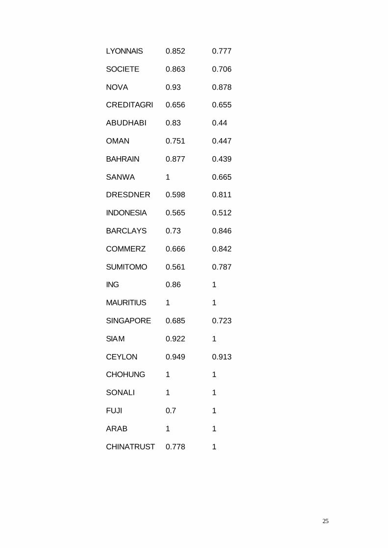
Attachment 1: Efficiency score of Indian banks in the year 1997-98
Efficiency Scores
Bank Model A Model B
SBI 1 1
SBH 0.93 0.611
SBP 0.924 0.56
SBT 0.877 0.555
SBBJ 0.866 0.581
SBM 0.829 0.544
SBS 0.803 0.588
SBIND 0.772 0.543
BOI 0.957 1
BOB 1 1
CANBANK 1 0.751
PNB 0.969 0.742
CBI 0.943 0.615
UBI 0.961 0.687
IOB 0.868 0.651
SYNBANK 0.895 0.564
INDBANK 0.674 0.651
UCO 0.786 0.488
ALLABANK 0.864 0.536
OBC 1 0.638
UNITED 0.87 0.28

23
DENA 0.909 0.614
CORPBANK 0.982 0.501
BOM 0.894 0.397
VIJAYA 0.798 0.391
ANDHRA 0.851 0.415
PSB 0.794 0.417
FEDERAL 0.847 0.623
VYASYA 0.81 0.458
JKBL 0.981 0.43
KNTBANK 0.9 0.511
BOR 0.731 0.475
BOMDR 0.703 0.431
SOUBANK 0.795 0.501
UWB 0.786 0.479
KARUR 0.816 0.496
CATHOLIC 0.734 0.494
TMB 0.859 0.452
DCB 0.812 0.482
LAXMIVILAS 0.693 0.463
BHARAT 0.776 0.382
SANGLI 0.713 0.271
DHANLAKSH 0.775 0.454
CITYUNION 0.768 0.462
NEDUNGADI 0.709 0.464
BENARES 0.625 0.217

24
LORD 0.782 0.427
NAINITAL 0.653 0.046
BAREILLY 0.561 0.065
RATNAKAR 0.583 0.15
GANESH 0.548 0.122
INDUSIND 1 1
GLOBAL 0.952 0.739
UTI 0.873 0.681
ICICI 0.874 0.486
TIMES 0.765 0.447
HDFC 0.887 0.364
IDBI 0.796 0.449
PUNJAB 0.766 0.852
CENTURIN 0.826 0.622
ANZ 1 0.696
CITI 1 1
HSBC 0.865 0.635
STANCHART 0.788 0.794
BOA 1 1
DEUTSCHE 1 1
AMEX 0.722 0.786
ABN 0.857 1
BRITISH 1 0.476
TOKYO 0.893 0.597
BNP 0.867 0.611
25
LYONNAIS 0.852 0.777
SOCIETE 0.863 0.706
NOVA 0.93 0.878
CREDITAGRI 0.656 0.655
ABUDHABI 0.83 0.44
OMAN 0.751 0.447
BAHRAIN 0.877 0.439
SANWA 1 0.665
DRESDNER 0.598 0.811
INDONESIA 0.565 0.512
BARCLAYS 0.73 0.846
COMMERZ 0.666 0.842
SUMITOMO 0.561 0.787
ING 0.86 1
MAURITIUS 1 1
SINGAPORE 0.685 0.723
SIAM 0.922 1
CEYLON 0.949 0.913
CHOHUNG 1 1
SONALI 1 1
FUJI 0.7 1
ARAB 1 1
CHINATRUST 0.778 1
Recommended